Gravitational wave peak luminosity model for precessing binary black holes

Abstract

When two black holes merge, a tremendous amount of energy is released in the form of gravitational radiation in a short span of time, making such events among the most luminous phenomenon in the universe. Models that predict the peak luminosity of black hole mergers are of interest to the gravitational wave community, with potential applications in tests of general relativity. We present a surrogate model for the peak luminosity that is directly trained on numerical relativity simulations of precessing binary black holes. Using Gaussian process regression, we interpolate the peak luminosity in the 7-dimensional parameter space of precessing binaries with mass ratios $q\leq 4$, and spin magnitudes $\chi_{1},\chi_{2}\leq 0.8$. We demonstrate that our errors in estimating the peak luminosity are lower than those of existing fitting formulae by about an order of magnitude. In addition, we construct a model for the peak luminosity of aligned-spin binaries with mass ratios $q\leq 8$, and spin magnitudes $|\chi_{1z}|,|\chi_{2z}|\leq 0.8$. We apply our precessing model to infer the peak luminosity of the GW event GW190521, and find the results to be consistent with previous predictions.

I Introduction

As the gravitational wave (GW) detectors LIGO Aasi et al. (2015) and Virgo Acernese et al. (2015) approach their design sensitivity, GW detections are becoming routine Abbott et al. (2018, 2020a, 2020b, 2020c, 2020d). Binary black hole (BBH) mergers are the most abundant source for these detectors. Such mergers provide a unique laboratory for studying black hole (BH) astrophysics as well as for testing general relativity. At the time of merger, the BHs are moving at about half the speed of light and the spacetime is highly dynamical. As a result, for a brief moment, BBH mergers are among the most luminous events in the universe. For example, the recently announced GW event GW190521 Abbott et al. (2020d) radiated $\sim 7.6M_{\odot}$ of energy in GWs in a fraction of a second, reaching a peak luminosity of $\sim 208\,M_{\odot}\,c^{2}/s=3.7\times 10^{56}$ erg/s Abbott et al. (2020e).

The above estimate is obtained by applying peak luminosity models Keitel et al. (2017); Healy and Lousto (2017) based on numerical relativity (NR) simulations to the measured masses and spins of the component BHs. Apart from predicting the peak luminosity of GW events, such models can be used to understand the impact of supermassive BH mergers on circumbinary accretion disks Schnittman (2013) and possible electromagnetic counterparts Kocsis and Loeb (2008); Li et al. (2012). In addition, one can test general relativity by independently estimating the peak luminosity through a theory-independent signal reconstruction Cornish and Littenberg (2015); Millhouse et al. (2018) and comparing with the prediction from NR. A similar test was performed for the peak frequency in Ref. Carullo et al. (2019). As detector sensitivity improves, these applications will need accurate models that capture the full physics of the NR simulations.

NR simulations are essential to model the BH merger process and the resulting GW peak luminosity. However, these are prohibitively expensive for most GW data analysis applications. As a result, various phenomenological fits have been developed for the peak luminosity Keitel et al. (2017); Healy and Lousto (2017); Jiménez Forteza et al. (2016); Baker et al. (2008); starting with an ansatze, these models calibrate any free coefficients to NR simulations. However, all of these models are restricted to aligned-spin systems, where the BH spins are aligned to the orbital angular momentum direction ($\hat{\bm{L}}$). For generic binaries, however, the spins can be titled w.r.t. $\hat{\bm{L}}$. For these systems, the spins interact with the orbit (and each other), leading to precession of the orbital plane and the spins Apostolatos et al. (1994). Precession causes modulations in the GW signal and as a result the peak luminosity is affected.

In this paper, we present a Gaussian process regression (GPR) based NR surrogate model for the peak luminosity of generically precessing BBHs. NR surrogate models directly interpolate between NR simulations rather than assume an ansatze about the underlying phenomenology. These methods have been successfully used to model the GW signal Varma et al. (2019a); Blackman et al. (2017a, b) as well as the remnant BH properties Varma et al. (2019b, a, 2020) of precessing BBHs. Through cross-validation studies, these models have been shown to approach the accuracy level of the NR simulations themselves.

In particular, we present two models:

1. NRSur7dq4Remnant: a 7-dimensional precessing model trained against systems with mass ratios $q\leq 4$,   dimensionless spin magnitudes $\chi_{1},\chi_{2}\leq 0.8$, and generic spins directions.

2. NRSur3dq8Remnant: a 3-dimensional aligned-spin model trained against systems with mass ratios up to $q\leq 8$ and aligned-spins $|\chi_{1z}|,|\chi_{2z}|\leq 0.8$.

We use the same names, respectively, as the precessing remnant model of Ref. Varma et al. (2019a) and the aligned-spin remnant model of Ref. Varma et al. (2019b), as we make the models available in the same interface through the publicly available Python module surfinBH Varma et al. . Even though peak luminosity is not technically a property of the remnant BH, we expect that using the same interface will make using the models easier for our users.

The rest of the paper is as follows. We describe our fitting procedure in Sec. II. In Sec. III, we compare the models against NR simulations to assess their accuracy. In Sec. IV, we apply our precessing model to predict the peak luminosity of GW190521. We end with some concluding remarks in Sec. V.

II Modeling methods

The GW luminosity is defined as Baker et al. (2008) :

$$\mathcal{L}(t)=\frac{1}{16\pi}\sum_{\ell,m}\left|\lim\limits_{r\to\infty}\left(r\,\dot{\mathpzc{h}}_{\ell m}\right)\right|^{2},$$ (1)

where the dot represents a time derivative, the $|~{}|$ represents the absolute value, and $\mathpzc{h}_{\ell m}$ represents the complex spin $\!=\!\!-2$ weighted spherical harmonic mode with indices $(\ell,m)$. We use the time derivative of $r\mathpzc{h}_{\ell m}$ extrapolated to future null infinity Boyle and Mroue (2009) in the place of $\lim\limits_{r\to\infty}\left(r\,\dot{\mathpzc{h}}_{\ell m}\right)$. The extrapolated strain data is obtained from NR simulations performed with the Spectral Einstein Code (SpEC) SpE code, available through the Simulating eXtreme Spacetimes (SXS) SXS Catalog Boyle et al. (2019a); SXS Collaboration . The strain data is first interpolated onto a uniform time array (with step size $0.1M$, where $M$ is the total mass) using cubic splines. Then we use a fourth-order finite-difference derivative to get the time derivative of the strain.

We determine the peak luminosity as

$$\mathcal{L}_{\mathrm{peak}}=\smash{\displaystyle\max_{t}}\,\mathcal{L}(t)\,,$$ (2)

where we determine the peak value by fitting a quadratic function to 5 adjacent samples of $\mathcal{L}(t)$, consisting of the largest sample and two neighbors on either side. Before applying our fitting method, we first take a logarithm of the peak luminosity and model $\log{(\mathcal{L}_{\mathrm{peak}})}$. We find that this leads to more accurate fits than directly modeling $\mathcal{L}_{\mathrm{peak}}$. When the model is evaluated, we can easily get the predicted peak luminosity by taking the exponential of the fit output.

For the aligned-spin model NRSur3dq8Remnant, we include the $\ell\leq 4$ and (5,5) modes but not the (4,1) or (4,0) modes in Eq. (1). We include the $m>0$ modes twice to account for the $m<0$ modes, which are given by $\mathpzc{h}_{\ell,-m}=(-1)^{\ell}\,\mathpzc{h}_{\ell m}^{*}$ due to the symmetries of aligned-spin systems. The included modes are the same as those used for the surrogate model of Ref. Varma et al. (2019c). The reason for excluding the (4,1), (4,0), $(\ell=5,m<5)$ and $\ell>5$ modes is two fold: (i) These modes have very small amplitudes and do not contribute significantly to the sum in Eq. (1). (ii) The small amplitude of some of these modes (particularly (4,1) and (4,0)) can behave poorly when extrapolated Boyle and Mroue (2009). We expect that this will be resolved in the future with Cauchy characteristic extraction Barkett et al. (2020); Moxon et al. (2020).

For the precessing model NRSur7dq4Remnant, we use all $\ell\leq 5$ modes. Due to the orbital precession, even modes like (4,1), (4,0) and $(\ell=5,m<5)$ can have significant amplitude due to mode mixing (see for e.g. Ref. Varma et al. (2019a)). Therefore, these modes behave reasonably well when extrapolated. Note that the $m<0$ modes are directly included when doing the sum in Eq. (1) as the aforementioned symmetry for $m<0$ does not hold for precessing systems.

II.1 Gaussian process regression

We construct fits in this work using GPR Rasmussen and Williams (2006) as implemented in scikit-learn Pedregosa et al. (2012). We closely follow the procedure outlined in the supplement of Ref. Varma et al. (2019b), which we describe briefly in the following.

We start with a training set of $n$ observations, $\mathcal{TS}=\left\{\bm{\Lambda}^{i},f(\bm{\Lambda}^{i}))|i=1,\dots,n\right\}$, where each $\bm{\Lambda}^{i}$ denotes an input vector of dimension $D$ and $f(\bm{\Lambda}^{i})$ is the corresponding scalar output. In our case, $\bm{\Lambda}$ is given by Eq.(6) and Eq.(11) respectively, for the precessing and aligned-spin models, and $f(\bm{\Lambda})=\log{(\mathcal{L}_{\mathrm{peak}})}$. Our goal is to use $\mathcal{TS}$ to make predictions for the underlying $f(\bm{\Lambda})$ at any point $\bm{\Lambda}_{*}$ that is not in $\mathcal{TS}$.

A Gaussian process (GP) can be thought of as a probability distribution of functions. More formally, a GP is a collection of random variables, any finite number of which have a joint Gaussian distribution Rasmussen and Williams (2006). A GP is completely specified by its mean function $m(\bm{\Lambda})$ and covariance function $k(\bm{\Lambda},\bm{\Lambda}^{\prime})$, i.e. $f(\bm{\Lambda})\sim\mathcal{GP}(m(\bm{\Lambda}),k(\bm{\Lambda},\bm{\Lambda}^{\prime}))$. Consider a prediction set of $n_{*}$ test inputs and their corresponding outputs (which are unknown): $\mathcal{PS}=\left\{(\bm{\Lambda}^{i}_{*},f(\bm{\Lambda}^{i}_{*}))|i=1,\dots,n_{*}\right\}$. By the definition of a GP, outputs of $\mathcal{TS}$ and $\mathcal{PS}$ (respectively ${\bf f}\!=\!\{f(\bm{\Lambda}^{i})\}$, ${\bf f_{*}}\!=\!\{f(\bm{\Lambda}^{i}_{*})\}$) are related by a joint Gaussian distribution:

$$\begin{bmatrix}{\bf{f}}\\ {\bf{f_{*}}}\end{bmatrix}=\mathcal{N}\left({\bf 0},\begin{bmatrix}K_{\bm{\Lambda}\bm{\Lambda}}&K_{\bm{\Lambda}\bm{\Lambda}_{*}}\\ K_{\bm{\Lambda}_{*}\bm{\Lambda}}&K_{\bm{\Lambda}_{*}\bm{\Lambda}_{*}}\end{bmatrix}\right),$$ (3)

where $K_{\bm{\Lambda}\bm{\Lambda}_{*}}$ denotes the $n\!\times\!n_{*}$ matrix of the covariance $k(\bm{\Lambda},\bm{\Lambda}_{*})$ evaluated at all pairs of training and prediction points, and similarly for the other $K$ matrices.

Eq. (3) provides the Bayesian prior distribution for ${\bf f_{*}}$. The posterior distribution is obtained by restricting this joint prior to contain only those functions which agree with the observed data points Rasmussen and Williams (2006), i.e.

$$p({\bf f_{*}}|\mathcal{TS})=\mathcal{N}\Bigg{(} K_{\bm{\Lambda}_{*}\bm{\Lambda}}~{}K_{\bm{\Lambda}\bm{\Lambda}}^{-1}~{}{\bf f}\,,$$

$$\,K_{\bm{\Lambda}_{*}\bm{\Lambda}_{*}}-K_{\bm{\Lambda}_{*}\bm{\Lambda}}~{}K_{\bm{\Lambda}\bm{\Lambda}}^{-1}~{}K_{\bm{\Lambda}\bm{\Lambda}_{*}}\Bigg{)}.$$ (4)

The mean of this posterior provides an estimator for $f(\bm{\Lambda})$ at $\bm{\Lambda}_{*}$, while its width is the prediction error.

Finally, one needs to specify the covariance (or kernel) function $k(\bm{\Lambda},\bm{\Lambda}^{\prime})$. Following Ref. Varma et al. (2019b), we implement the following kernel

$$k(\bm{\Lambda},\bm{\Lambda}^{\prime})=\sigma_{k}^{2}\exp{\left[\!-\sum_{j=1}^{D}\left(\frac{\bm{\Lambda}^{j}\!-\!\bm{\Lambda}^{\prime j}}{\sqrt{2}\,\sigma_{j}}\right)^{2}\!\right]}+\sigma_{n}^{2}\,\delta_{\bm{\Lambda}\bm{\Lambda}^{\prime}}\,,$$ (5)

where $\delta_{\bm{\Lambda}\bm{\Lambda}^{\prime}}$ is the Kronecker delta. In words, we use a product between a squared exponential kernel (parametrized by $\sigma_{j}$) and a constant kernel (parametrized by $\sigma_{k}^{2}$), to which we add a white kernel (parametrized by $\sigma_{n}^{2}$) to account for additional noise in the training data Rasmussen and Williams (2006); Pedregosa et al. (2012).

GPR fit construction involves determining the $D\!+\!2$ hyperparameters ($\sigma_{k}$, $\sigma_{n}$ and $\sigma_{j}$) which maximize the marginal likelihood of the training data under the GP prior Rasmussen and Williams (2006). Local maxima are avoided by repeating the optimization with 10 different initial guesses, obtained by sampling uniformly in log in the hyperparameter space described below.

Before constructing the GPR fit, we pre-process the training data as follows. We first subtract a linear fit and the mean of the resulting values. The data are then normalized by dividing by the standard deviation of the resulting values. The inverse of these transformations is applied at the time of the fit evaluation. The reasoning behind the pre-processing is two-fold: (1) The de-meaning and normalization allows us to apply the same ranges (described below) for the GPR hyperparameters for a wide range of models. For instance, we used the same settings to model the remnant BH properties in Refs. Varma et al. (2019b, a). (2) The data are simpler to model after removing the linear component, leading to more accurate fits.

For each dimension of $\bm{\Lambda}$, we define $\Delta\bm{\Lambda}^{j}$ to be the range of the values of $\bm{\Lambda}^{j}$ in $\mathcal{TS}$ and consider $\sigma_{j}\in[0.01\times\Delta\bm{\Lambda}^{j},10\times\Delta\bm{\Lambda}^{j}]$. Larger length scales are unlikely to be relevant and smaller length scales are unlikely to be resolvable. The remaining hyperparameters are sampled in $\sigma_{k}^{2}\in[10^{-2},10^{2}]$ and $\sigma_{n}^{2}\in[10^{-7},10^{-2}]$. These choices are meant to be conservative and are based on prior exploration of the typical magnitude and noise level in our training data.

II.2 Precessing model, NRSur7dq4Remnant

For precessing systems the parameter space is 7-dimensional comprising of the mass $q$, and two spin 3-vectors $\bm{\chi}_{1}$ and $\bm{\chi}_{2}$. Here $q=m_{1}/m_{2}$ is the mass ratio with $m_{1}\geq m_{2}$, and $\bm{\chi}_{1}$ ($\bm{\chi}_{2}$) is the dimensionless spin vector of the heavier (lighter) BH. The total mass ($M=m_{1}+m_{2}$) scales out of the problem and does not constitute an additional parameter for modeling. We use the 1528 NR waveforms used for the surrogate models of Ref. Varma et al. (2019a), which cover the parameter space $q\leq 4$, $\chi_{1},\chi_{2}\leq 0.8$, where $\chi_{1}$ ($\chi_{2}$) is the magnitude of $\bm{\chi}_{1}$ ($\bm{\chi}_{2}$).

Following Refs. Varma et al. (2019a, b), we parametrize the precessing fit using the coorbital frame spins $\bm{\chi}^{\mathrm{coorb}}_{1,2}$ at $t\!=\!-100M$ before the peak of the total waveform amplitude (as defined in Eq. 5 of Ref. Varma et al. (2019a)). The coorbital frame is a time-dependent non-inertial frame in which the $z-$axis is along the instantaneous $\hat{\bm{L}}$ direction, and $x-$axis is along the instantaneous line-of-separation between the BHs, with the heavier BH on the positive $x-$axis. The NRSur7dq4Remnant fit is parametrized as follows.

$$\bm{\Lambda}=[\log(q),\chi^{\mathrm{coorb}}_{1x},\chi^{\mathrm{coorb}}_{1y},\hat{\chi}^{\mathrm{coorb}},\chi^{\mathrm{coorb}}_{2x},\chi^{\mathrm{coorb}}_{2y},\chi^{\mathrm{coorb}}_{a}],$$ (6)

where $\hat{\chi}^{\mathrm{coorb}}$ is the spin parameter entering the GW phase at leading order Khan et al. (2016); Ajith (2011); Cutler and Flanagan (1994); Poisson and Will (1995) in the PN expansion

$$\hat{\chi}^{\mathrm{coorb}}=\frac{\chi^{\mathrm{coorb}}_{\mathrm{eff}}-38\eta(\chi^{\mathrm{coorb}}_{1z}+\chi^{\mathrm{coorb}}_{2z})/113}{1-{76\eta}/{113}}\,,$$ (7)

$$\chi^{\mathrm{coorb}}_{\mathrm{eff}}=\frac{q~{}\chi^{\mathrm{coorb}}_{1z}+\chi^{\mathrm{coorb}}_{2z}}{1+q},$$ (8)

$$\eta=\frac{q}{(1+q)^{2}}\,,$$ (9)

and $\chi^{\mathrm{coorb}}_{a}$ is the “anti-symmetric spin”,

$$\chi^{\mathrm{coorb}}_{a}=\tfrac{1}{2}(\chi^{\mathrm{coorb}}_{1z}-\chi^{\mathrm{coorb}}_{2z})\,.$$ (10)

We empirically found this parameterization to perform more accurately than the more intuitive choice $\tilde{\bm{\Lambda}}=[q,\chi^{\mathrm{coorb}}_{1x},\chi^{\mathrm{coorb}}_{1y},\chi^{\mathrm{coorb}}_{1z},\chi^{\mathrm{coorb}}_{2x},\chi^{\mathrm{coorb}}_{2y},\chi^{\mathrm{coorb}}_{2z}]$ used in Ref. Blackman et al. (2017a).

II.3 Aligned-spin model, NRSur3dq8Remnant

NRSur7dq4Remnant is restricted to $q\leq 4$ due to a lack of sufficient precessing simulations at higher mass ratios Boyle et al. (2019a). NR simulations become increasingly expensive as one approaches higher mass ratios and/or spin magnitudes. However, the SXS Catalog has good coverage for aligned-spin BBHs up to $q\leq 8$ Varma et al. (2019c); Boyle et al. (2019a). We make use of the 104 NR waveforms used for the surrogate model of Ref. Varma et al. (2019c), which cover the parameter space $q\leq 8$, $|\chi_{1z}|,|\chi_{2z}|\leq 0.8$.

Note that the spins in aligned-spin BBHs are restricted to the $\hat{\bm{L}}$ direction, this reduces the parameter space to 3-dimensions. Following Refs. Varma et al. (2019b, c), we parametrize the NRSur3dq8Remnant fit as follows.

$$\bm{\Lambda}=[\log(q),\hat{\chi}^{\mathrm{coorb}},\chi^{\mathrm{coorb}}_{a}],$$ (11)

where, we use Eq. (7) and (10), but keeping in mind that spins in the coorbital-frame are the same as those in the inertial frame for aligned-spin systems.

III Modeling errors

We evaluate the accuracy of our new surrogate models by comparing against the the NR simulations used in this work. To avoid underestimating the errors, we perform a 20-fold cross-validation study to compute “out-of-sample” errors as follows. We first randomly divide the training simulations into 20 groups of roughly the same size. For each group, we build a trial surrogate using the remaining training simulations and test against the simulations in that group, which may include points on the boundary of the training set.

For comparison, we also compute the errors for existing peak luminosity fitting formulae Keitel et al. (2017); Healy and Lousto (2017); Jiménez Forteza et al. (2016) against the NR simulations. We refer to the fit of Ref. Keitel et al. (2017) as UIB , the fit of Ref. Healy and Lousto (2017) as HL , and the fit of Ref. Jiménez Forteza et al. (2016) as FK . Note that these fits are not trained on precessing simulations. As the spins evolve for precessing systems, there is an ambiguity about at what time these fits should be evaluated. We follow the procedure outlined in Ref. Johnson-McDaniel et al. (2016) and used in LIGO/Virgo analyses (e.g. Abbott et al. (2020d)): NR spins are evolved from relaxation to the Schwarzschild innermost stable circular orbit (ISCO) using post-Newtonian (PN) theory. The spins at ISCO, projected along $\hat{\bm{L}}$, are used to evaluate the aligned-spin peak luminosity fitting formulae.

III.1 Errors for the precessing model

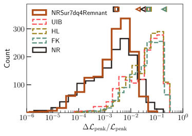
Figure 1: Fractional errors (out-of-sample) in predicting the peak luminosity for the precessing model NRSur7dq4Remnant when compared against precessing NR simulations. When evaluating NRSur7dq4Remnant, we use the NR spins at $t\!=\!-100M$, where the model was trained. Also shown are the NR resolution errors and errors for different existing fitting formulae. The square (triangle) markers at the top indicate the median (95th percentile) values. NRSur7dq4Remnant is more accurate than the existing formulae by about an order of magnitude.

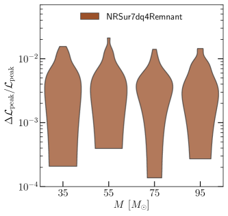
Figure 2: Fractional errors for NRSur7dq4Remnant in predicting the peak luminosity when spins are specified at a reference frequency of $f_{\mathrm{ref}}=20$ Hz. For four different total masses, we compute the errors against 23 long NR simulations that were not used to train the model. For each mass, the errors are shown as a smoothed vertical histogram (or a violin). The histograms are normalized so that all violins have equal width.

We demonstrate the accuracy of the NRSur7dq4Remnant model by comparing against the 1528 precessing NR simulations described in Sec. II.2. We perform a 20-fold cross-validation study where we leave out $\sim 75$ simulations in each trial for testing. Figure. 1 shows the errors for NRSur7dq4Remnant when using the NR spins at $t\!=\!-100M$ as the input. As the model was trained at this time, these errors represent the errors in the GPR fitting procedure. The 95th percentile fractional error in predicting the peak luminosity is $\mathchar 21016\relax\,0.02$. We also show the errors for existing fitting formulae, and the NR resolution error, estimated by comparing the two highest resolution simulations. Our errors are at the same level as the estimated NR error, and about an order of magnitude smaller than that of existing fitting formulae.

In practice, one might want to specify the input spins at arbitrary times. For example, in LIGO-Virgo analyses (e.g. Abbott et al. (2018)) the spins are measured at a fixed reference frequency. Following Refs. Varma et al. (2019b, a) this is handled by evolving the input spins from the reference frequency to $t\!=\!-100M$ using a combination of PN in the early inspiral and NRSur7dq4 Varma et al. (2019a) spin evolution in the late inspiral. Figure 2 shows the errors in NRSur7dq4Remnant when the spins are specified at a reference orbital frequency $f_{\mathrm{ref}}=20$ Hz. These errors are computed by comparing against 23 long NR ($3\times 10^{4}M$ to $10^{5}M$ in length) simulations Boyle et al. (2019b); Varma et al. (2019a) with mass ratios $q\leq 4$ and generically oriented spins with magnitudes $\chi_{1},\chi_{2}\sim 0.5$. Note that none of these simulations were used to train the surrogates. Comparing with Fig. 1, even with spin evolution, our errors are about an order of magnitude lower than that of existing fits.

III.2 Errors for the aligned-spin model

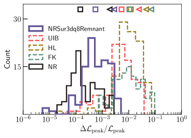
Figure 3: Fractional errors (out-of-sample) in predicting the peak luminosity for the aligned-spin model NRSur3dq8Remnant when compared against aligned-spin NR simulations. Also shown are the NR resolution errors and errors for different existing fitting formulae. The square (triangle) markers at the top indicate the median (95th percentile) values. NRSur3dq8Remnant is more accurate than the existing formulae by at least an order of magnitude.

We demonstrate the accuracy of the NRSur3dq8Remnant model by comparing against the 104 aligned-spin NR simulations described in Sec. II.3. We perform a 20-fold cross-validation study where we leave out $\sim 5$ simulations in each trial for testing. These errors are shown in Fig. 3. The 95th percentile fractional error in predicting the peak luminosity is $\mathchar 21016\relax\,0.002$. Fig. 3 also shows the errors for the existing fitting formulae and the estimated NR errors. NRSur3dq8Remnant is comparable to NR and more accurate than existing fits by at least an order of magnitude.

We note that the estimated NR errors for aligned-spin BBHs (Fig. 3) are significantly smaller than that for precessing BBHs (Fig. 1). The reason for this is not clear, but this places a limit on how accurate the surrogate models can be. This is reflected in the higher errors for NRSur7dq4Remnant compared to NRSur3dq8Remnant. More accurate precessing NR simulations may be necessary to further improve the precessing model.

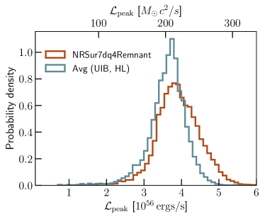
Figure 4: Posterior distribution for the peak luminosity of GW190521, obtained using the NRSur7dq4Remnant model as well as the average of the UIB Keitel et al. (2017) and HL Healy and Lousto (2017) fitting formulae. While the two posteriors are consistent with each other, NRSur7dq4Remnant suggests a slightly higher value for the peak luminosity.

IV Peak luminosity of GW190521

As a first application of our models, we compute the peak luminosity of GW190521 Abbott et al. (2020d) using NRSur7dq4Remnant. We apply the NRSur7dq4Remnant model to the posteriors samples for the component masses and spins, obtained using the preferred NRSur7dq4 model in Ref. Abbott et al. (2020e), and made publicly available Collaboration and Collaboration by the LIGO-Virgo Collaboration. This peak luminosity posterior is shown in Fig. 4. We compare this with the peak luminosity posterior obtained in Ref. Abbott et al. (2020e) using the average of the UIB Keitel et al. (2017) and HL Healy and Lousto (2017) fitting formulae applied to the same NRSur7dq4 posterior samples. While the two posteriors are consistent with each other, NRSur7dq4Remnant shows support for slightly higher values of peak luminosity. This level of agreement is expected, as GW190521 had a relatively weak signal-to-noise ratio of $\mathchar 21016\relax\,14.7$ Abbott et al. (2020d). As GW detectors become more sensitive in the coming years, we can expect to see stronger signals for which systematic biases in peak luminosity models will become important.

V Conclusion

We present GPR based NR surrogate models for peak luminosity of BBH mergers. The first model, NRSur7dq4Remnant, is trained on 1528 precessing systems with mass ratios $q\leq 4$ and spin magnitudes $\chi_{1},\chi_{2}\leq 0.8$. The second model, NRSur3dq8Remnant, is trained on 104 aligned-spin systems with mass ratios $q\leq 8$ and spins $|\chi_{1z}|,|\chi_{2z}|\leq 0.8$. Both models are comparable to the NR simulations in accuracy, and outperform existing fitting formulate by an order of magnitude or more. The models are made publicly available through the Python module surfinBH Varma et al. and can be used to estimate the peak luminosity of GW signals. We use NRSur7dq4Remnant to infer the peak luminosity of the GW event GW190521, and find the results to be consistent with previous predictions.

As our GW detectors improve, we will need models that capture the full physics of BBH mergers. NRSur7dq4Remnant is the first peak luminosity model trained on precessing NR simulations. Models such as this will become necessary to accurately infer the peak luminosity as we approach the era of high-precision GW astronomy.

References

References

- Aasi et al. (2015) J. Aasi et al. (LIGO Scientific), “Advanced LIGO,” Class. Quant. Grav. 32, 074001 (2015), arXiv:1411.4547 [gr-qc] .
- Acernese et al. (2015) F. Acernese et al. (Virgo), “Advanced Virgo: a second-generation interferometric gravitational wave detector,” Class. Quant. Grav. 32, 024001 (2015), arXiv:1408.3978 [gr-qc] .
- Abbott et al. (2018) B. P. Abbott et al. (LIGO Scientific, Virgo), “GWTC-1: A Gravitational-Wave Transient Catalog of Compact Binary Mergers Observed by LIGO and Virgo during the First and Second Observing Runs,” (2018), arXiv:1811.12907 [astro-ph.HE] .
- Abbott et al. (2020a) B.P. Abbott et al. (LIGO Scientific, Virgo), “GW190425: Observation of a Compact Binary Coalescence with Total Mass ,” Astrophys. J. Lett. 892, L3 (2020a), arXiv:2001.01761 [astro-ph.HE] .
- Abbott et al. (2020b) R. Abbott et al. (LIGO Scientific, Virgo), “GW190412: Observation of a Binary-Black-Hole Coalescence with Asymmetric Masses,” Phys. Rev. D 102, 043015 (2020b), arXiv:2004.08342 [astro-ph.HE] .
- Abbott et al. (2020c) R. Abbott et al. (LIGO Scientific, Virgo), “GW190814: Gravitational Waves from the Coalescence of a 23 Solar Mass Black Hole with a 2.6 Solar Mass Compact Object,” Astrophys. J. Lett. 896, L44 (2020c), arXiv:2006.12611 [astro-ph.HE] .
- Abbott et al. (2020d) R. Abbott et al. (LIGO Scientific, Virgo), “GW190521: A Binary Black Hole Merger with a Total Mass of ,” Phys. Rev. Lett. 125, 101102 (2020d), arXiv:2009.01075 [gr-qc] .
- Abbott et al. (2020e) R. Abbott et al. (LIGO Scientific, Virgo), “Properties and astrophysical implications of the 150 Msun binary black hole merger GW190521,” Astrophys. J. Lett. 900, L13 (2020e), arXiv:2009.01190 [astro-ph.HE] .
- Keitel et al. (2017) David Keitel et al., “The most powerful astrophysical events: Gravitational-wave peak luminosity of binary black holes as predicted by numerical relativity,” Phys. Rev. D 96, 024006 (2017), arXiv:1612.09566 [gr-qc] .
- Healy and Lousto (2017) James Healy and Carlos O. Lousto, “Remnant of binary black-hole mergers: New simulations and peak luminosity studies,” Phys. Rev. D95, 024037 (2017), arXiv:1610.09713 [gr-qc] .
- Schnittman (2013) Jeremy D. Schnittman, “Astrophysics of Super-massive Black Hole Mergers,” Class. Quant. Grav. 30, 244007 (2013), arXiv:1307.3542 [gr-qc] .
- Kocsis and Loeb (2008) Bence Kocsis and Abraham Loeb, “Brightening of an Accretion Disk Due to Viscous Dissipation of Gravitational Waves During the Coalescence of Supermassive Black Holes,” Phys. Rev. Lett. 101, 041101 (2008), arXiv:0803.0003 [astro-ph] .
- Li et al. (2012) Gongjie Li, Bence Kocsis, and Abraham Loeb, “Gravitational Wave Heating of Stars and Accretion Disks,” Mon. Not. Roy. Astron. Soc. 425, 2407–2412 (2012), arXiv:1203.0317 [astro-ph.HE] .
- Cornish and Littenberg (2015) Neil J. Cornish and Tyson B. Littenberg, “BayesWave: Bayesian Inference for Gravitational Wave Bursts and Instrument Glitches,” Class. Quant. Grav. 32, 135012 (2015), arXiv:1410.3835 [gr-qc] .
- Millhouse et al. (2018) Margaret Millhouse, Neil J. Cornish, and Tyson Littenberg, “Bayesian reconstruction of gravitational wave bursts using chirplets,” Phys. Rev. D 97, 104057 (2018), arXiv:1804.03239 [gr-qc] .
- Carullo et al. (2019) Gregorio Carullo, Gunnar Riemenschneider, Ka Wa Tsang, Alessandro Nagar, and Walter Del Pozzo, “GW150914 peak frequency: a novel consistency test of strong-field General Relativity,” Class. Quant. Grav. 36, 105009 (2019), arXiv:1811.08744 [gr-qc] .
- Jiménez Forteza et al. (2016) Xisco Jiménez Forteza, David Keitel, Sascha Husa, Mark Hannam, Sebastian Khan, Lionel London, and Michael Pürrer, Phenomenological fit of the peak luminosity from non-precessing binary-black-hole coalescences, Tech. Rep. LIGO-T1600018 (2016) https://dcc.ligo.org/LIGO-T1600018-v4/public.
- Baker et al. (2008) John G. Baker, William D. Boggs, Joan Centrella, Bernard J. Kelly, Sean T. McWilliams, and James R. van Meter, “Mergers of non-spinning black-hole binaries: Gravitational radiation characteristics,” Phys. Rev. D 78, 044046 (2008), arXiv:0805.1428 [gr-qc] .
- Apostolatos et al. (1994) Theocharis A. Apostolatos, Curt Cutler, Gerald J. Sussman, and Kip S. Thorne, “Spin-induced orbital precession and its modulation of the gravitational waveforms from merging binaries,” Phys. Rev. D 49, 6274–6297 (1994).
- Varma et al. (2019a) Vijay Varma, Scott E. Field, Mark A. Scheel, Jonathan Blackman, Davide Gerosa, Leo C. Stein, Lawrence E. Kidder, and Harald P. Pfeiffer, “Surrogate models for precessing binary black hole simulations with unequal masses,” Phys. Rev. Research. 1, 033015 (2019a), arXiv:1905.09300 [gr-qc] .
- Blackman et al. (2017a) Jonathan Blackman, Scott E. Field, Mark A. Scheel, Chad R. Galley, Christian D. Ott, Michael Boyle, Lawrence E. Kidder, Harald P. Pfeiffer, and Béla Szilágyi, “Numerical relativity waveform surrogate model for generically precessing binary black hole mergers,” Phys. Rev. D96, 024058 (2017a), arXiv:1705.07089 [gr-qc] .
- Blackman et al. (2017b) Jonathan Blackman, Scott E. Field, Mark A. Scheel, Chad R. Galley, Daniel A. Hemberger, Patricia Schmidt, and Rory Smith, “A Surrogate Model of Gravitational Waveforms from Numerical Relativity Simulations of Precessing Binary Black Hole Mergers,” Phys. Rev. D95, 104023 (2017b), arXiv:1701.00550 [gr-qc] .
- Varma et al. (2019b) Vijay Varma, Davide Gerosa, Leo C. Stein, François Hébert, and Hao Zhang, “High-accuracy mass, spin, and recoil predictions of generic black-hole merger remnants,” Phys. Rev. Lett. 122, 011101 (2019b), arXiv:1809.09125 [gr-qc] .
- Varma et al. (2020) Vijay Varma, Maximiliano Isi, and Sylvia Biscoveanu, “Extracting the Gravitational Recoil from Black Hole Merger Signals,” Phys. Rev. Lett. 124, 101104 (2020), arXiv:2002.00296 [gr-qc] .
- (25) V. Varma et al., “surfinBH,” pypi.org/project/surfinBH, doi.org/10.5281/zenodo.1418525.
- Boyle and Mroue (2009) Michael Boyle and Abdul H. Mroue, “Extrapolating gravitational-wave data from numerical simulations,” Phys. Rev. D80, 124045 (2009), arXiv:0905.3177 [gr-qc] .
- (27) “The Spectral Einstein Code,” http://www.black-holes.org/SpEC.html.
- (28) “Simulating eXtreme Spacetimes,” http://www.black-holes.org/.
- Boyle et al. (2019a) Michael Boyle et al., “The SXS Collaboration catalog of binary black hole simulations,” Class. Quant. Grav. 36, 195006 (2019a), arXiv:1904.04831 [gr-qc] .
- (30) SXS Collaboration, “The SXS collaboration catalog of gravitational waveforms,” http://www.black-holes.org/waveforms.
- Varma et al. (2019c) Vijay Varma, Scott E. Field, Mark A. Scheel, Jonathan Blackman, Lawrence E. Kidder, and Harald P. Pfeiffer, “Surrogate model of hybridized numerical relativity binary black hole waveforms,” Phys. Rev. D 99, 064045 (2019c), arXiv:1812.07865 [gr-qc] .
- Barkett et al. (2020) Kevin Barkett, Jordan Moxon, Mark A. Scheel, and Béla Szilágyi, “Spectral Cauchy-Characteristic Extraction of the Gravitational Wave News Function,” Phys. Rev. D 102, 024004 (2020), arXiv:1910.09677 [gr-qc] .
- Moxon et al. (2020) Jordan Moxon, Mark A. Scheel, and Saul A. Teukolsky, “Improved Cauchy-characteristic evolution system for high-precision numerical relativity waveforms,” Phys. Rev. D 102, 044052 (2020), arXiv:2007.01339 [gr-qc] .
- Rasmussen and Williams (2006) C. E. Rasmussen and C. K. I. Williams, Gaussian Processes for Machine Learning, by C.E. Rasmussen and C.K.I. Williams. ISBN-13 978-0-262-18253-9 (2006).
- Pedregosa et al. (2012) F. Pedregosa, G. Varoquaux, A. Gramfort, V. Michel, B. Thirion, O. Grisel, M. Blondel, A. Müller, J. Nothman, G. Louppe, P. Prettenhofer, R. Weiss, V. Dubourg, J. Vanderplas, A. Passos, D. Cournapeau, M. Brucher, M. Perrot, and É. Duchesnay, “Scikit-learn: Machine Learning in Python,” Journal of Machine Learning Research 12, 2825–2830 (2012), 1201.0490 .
- Khan et al. (2016) Sebastian Khan, Sascha Husa, Mark Hannam, Frank Ohme, Michael Pürrer, Xisco Jiménez Forteza, and Alejandro Bohé, “Frequency-domain gravitational waves from nonprecessing black-hole binaries. II. A phenomenological model for the advanced detector era,” Phys. Rev. D93, 044007 (2016), arXiv:1508.07253 [gr-qc] .
- Ajith (2011) P. Ajith, “Addressing the spin question in gravitational-wave searches: Waveform templates for inspiralling compact binaries with nonprecessing spins,” Phys. Rev. D 84, 084037 (2011), arXiv:1107.1267 [gr-qc] .
- Cutler and Flanagan (1994) Curt Cutler and Eanna E. Flanagan, “Gravitational waves from merging compact binaries: How accurately can one extract the binary’s parameters from the inspiral wave form?” Phys. Rev. D49, 2658–2697 (1994), arXiv:gr-qc/9402014 [gr-qc] .
- Poisson and Will (1995) Eric Poisson and Clifford M. Will, “Gravitational waves from inspiraling compact binaries: Parameter estimation using second postNewtonian wave forms,” Phys. Rev. D52, 848–855 (1995), arXiv:gr-qc/9502040 [gr-qc] .
- Johnson-McDaniel et al. (2016) Nathan K. Johnson-McDaniel, Anuradha Gupta, P Ajith, David Keitel, Ofek Birnholtz, Frank Ohme, and Sascha Husa, Determining the final spin of a binary black hole system including in-plane spins: Method and checks of accuracy, Tech. Rep. LIGO-T1600168 (2016) https://dcc.ligo.org/LIGO-T1600168/public.
- Boyle et al. (2019b) Michael Boyle et al., “The SXS Collaboration catalog of binary black hole simulations,” (2019b), arXiv:1904.04831 [gr-qc] .
- (42) LIGO Scientific Collaboration and Virgo Collaboration, “Gravitational Wave Open Science Center,” https://www.gw-openscience.org.