Stability analysis of a singlerate and multirate predictor-corrector scheme for overlapping grids

Abstract

We use matrix stability analysis for a singlerate and multirate predictor-corrector scheme (PC) used to solve the incompressible Navier-Stokes equations (INSE) in overlapping grids. By simplifying the stability analysis with the unsteady heat equation in 1D, we demonstrate that, as expected, the stability of the PC scheme increases with increase in the resolution and overlap of subdomains. For singlerate timestepping, we also find that the high-order PC scheme is stable when the number of corrector iterations ($Q$) is odd. This difference in the stability of odd- and even-$Q$ is novel and has not been demonstrated in the literature for overlapping grid-based methods. We address the odd-even behavior in the stability of the PC scheme by modifying the last corrector iterate, which leads to a scheme whose stability increases monotonically with $Q$. For multirate timestepping, we observe that the stability of the PC scheme depends on the timestep ratio ($\eta$). For $\eta=2$, even-$Q$ is more stable than odd-$Q$. For $\eta\geq 3$, even-$Q$ is more stable than odd-$Q$ for a small nondimensional timestep size and the odd-even behavior vanishes as the timestep size increases. The stability analysis presented in this work gives novel insight into a high-order temporal discretization for ODEs and PDEs, and has helped us develop an improved PC scheme for solving the incompressible Navier-Stokes equations.

1 Introduction

Numerical solution of partial differential equations (PDEs) is central to much of today’s engineering analysis and scientific inquiry. Techniques such as the finite element method (FEM), the finite volume method (FVM), and the spectral element method (SEM) are used to approximate solutions of PDEs on a collection of volumes or elements whose union constitutes a mesh that covers the entire computational domain, $\Omega$. Construction of an optimal mesh (grid) is not a trivial task and often becomes a bottleneck for complex domains. Overlapping Schwarz (OS) based methods circumvent issues posed by conformal grids by allowing the domain to be represented as the union of simpler subdomains, each of which can be meshed independently with relatively simple mesh constructions. The nonconforming union of these meshes allows combinations of local mesh topologies that are otherwise incompatible, which is a feature of particular importance for complex 3D domains. As a results, OS-based methods have become popular for solving different classes of problems such as incompressible flow [1, 2, 3, 4, 5], compressible flow [6, 7, 8, 9, 10], electromagnetics [11, 12], heat transfer [13, 14, 15], and particle tracking [16], and have been implemented using various discretization approaches such as the finite difference method (FD), FEM, FVM, and SEM.

The focus of this work is the stability of the temporal discretization used in the Schwarz-SEM framework for solving the incompressible Navier-Stokes equations (INSE) on overlapping grids [1, 17, 18, 19]. The Schwarz-SEM framework is based on the spectral element method for monodomain conforming meshes [20, 21], which has demonstrated exponential convergence of the solution (with the order of the polynomial used for quadrature on each element) and up to third-order temporal convergence. The Schwarz-SEM framework uses a high-order spatial interpolation approach [1] for exchanging overlapping grid solution to maintain the exponential convergence and a high-order predictor-corrector (PC) timestepping approach to maintain the temporal convergence of the underlying SEM solver. The spatial and temporal discretization used in the Schwarz-SEM framework brings forth several considerations from a stability, accuracy, and computational-cost point of view. These factors include the extrapolation order used for the interdomain boundary data at the predictor step, the number of corrector (Schwarz) iterations at each timestep, and the amount of grid overlap required between adjacent subdomains. Here, we present stability analysis to understand how each of these factors impact the singlerate and multirate predictor-corrector scheme used in the Schwarz-SEM framework, and develop a more efficient timestepping approach for the INSE.

Since analysing the stability of the incompressible Navier-Stokes equations in two- or three-dimensions is not straightforward due to the complexity of the PDE, we simplify our analysis by considering the unsteady heat equation in 1D using the finite difference (FD) method. We specifically choose the unsteady heat equation due to the similarity in the eigenvalue spectrum of the diffusion operator and the parabolic unsteady Stokes operator, and use the matrix method for stability analysis [22] to analyze the predictor-corrector scheme of the Schwarz-SEM framework. PC schemes have been analyzed extensively for differential equations with some of the earliest work done dating back to 1960s [23, 24, 25], but their understanding in the context of overlapping grids is limited. Peet et al. [26] use matrix method for stability analysis to study a singlerate-based PC scheme for overlapping grids, but their results fail to describe certain aspects of the stability behavior that we have observed in the Schwarz-SEM framework. Mathew et al. [27] and Wu et al. [28] use theoretical analysis to understand stability behavior of their methods for solving PDEs on overlapping grids, but their method is based on a different temporal discretization compared to the BDF$k$/EXT$m$-based predictor-corrector scheme that we are interested in. Meng et al.’s conjugate heat transfer method [13] focuses on nonoverlapping fluid-solid interfaces and have different boundary conditions (mixed Dirichlet and Neumann) compared to the Schwarz-SEM framework (purely Dirichlet). Love et al. have analyzed a midpoint-based predictor-corrector scheme for Lagrangian shock hydrodynamics, where they demonstrate a difference in the stability of odd and even corrector iterates [29]. While the temporal discretization used by Love et al. is different from our method, their result on the difference in stability of odd and even iterate is similar to what we have observed in the Schwarz-SEM framework. We have also found similar evidence of difference in the stability of odd- and even-iterates of high-order predictor-corrector schemes in the context of ODEs (Fig. 3.2.4 in [21] and Fig. 1 in [30]). In [30], Stetter has analyzed an third-order accurate Adam Bashforth- (AB) and second-order accurate Adam-Moulton-based (AM) method for ODE of the form $\frac{\partial y}{\partial t}=\lambda y$ and the stability results therein indicate that the high-order PC scheme is relatively more stable for odd-iterates when $\lambda$ is real-valued. While this observation is not a part of Stetter’s discussion, empirical evidence in our work shows that this behavior might be applicable to high-order PC schemes in general when $\lambda$ is real-valued.

The results presented in this paper provide novel insight into the stability characteristics of a singlerate and multirate predictor-corrector scheme for overlapping grids. We also develop an improved PC scheme for singlerate timestepping that addresses the shortcomings in the stability characteristics of the existing PC scheme. The remainder of the paper is organized as follows. Section 2 introduces the matrix method for stability analysis, the overlapping Schwarz method for solving PDEs, and the FD-based discretization for solving the unsteady heat equation in a 1D monodomain grid. In Section 3, we extend the solution of the unsteady heat equation in a monodomain to overlapping grids using the singlerate and multirate predictor-corrector scheme from the Schwarz-SEM framework. In Section 4, we analyze the stability of the singlerate PC scheme and demonstrate that our simplified analysis qualitatively captures the stability behavior that we have observed in the Schwarz-SEM framework. Here, we also developed an improved PC scheme for singlerate timestepping. In Section 5, we analyze the multirate PC scheme for an arbitrary timestep ratio. Finally in Section 6, we summarize our findings and discuss possible directions for future work.

2 Preliminaries

In this section, we introduce the matrix method for stability analysis, summarize the overlapping Schwarz method for solving PDEs in overlapping subdomains, and describe our temporal and spatial discretization for solving the unsteady heat equation in a single conforming grid.

2.1 Matrix method for stability analysis

In the matrix method for stability analysis [22], if the system of equations to advance the solution in time can be represented as

$$u^{n}=Gu^{n-1},$$ (1)

where $u^{n}$ denotes the solution $u$ at time $t^{n}$, a sufficient and necessary condition for stability is that the spectral radius of the propogation operator is $\rho(G)<1$. For our stability analysis, we represent our predictor-corrector scheme into a system of this form (1) and use the spectral radius of $G$ to understand how various factors of interest impact the stability of the method. We also use this approach to design a novel singlerate PC scheme that significantly improves the stability characteristics of the current method (Section 4).

2.2 Overlapping Schwarz method

The OS method for solving a PDE in overlapping domains was introduced by Schwarz in 1870 [31]. Figure 1 shows the composite domain $\Omega$ used in Schwarz’s initial model problem, which is partitioned into two overlapping subdomains: a rectangle ($\Omega^{1}$) and a circle ($\Omega^{2}$). We use $\partial\Omega^{s}_{I}$ to denote the “interdomain boundary”, namely the segment of the subdomain boundary $\partial\Omega^{s}$ that is interior to another subdomain, and these interdomain boundaries $\partial\Omega^{1}_{I}$ and $\partial\Omega^{2}_{I}$ are highlighted in Fig. 1(b).

$\begin{array}[]{cc}\includegraphics[height=122.34685pt]{figures/schwarzmono}&\hskip 5.69054pt\includegraphics[height=128.0374pt]{figures/schwarzreccir}\end{array}$

Figure 1: (left to right) (a) Composite domain $\Omega$ (b) modeled by overlapping rectangular ($\Omega^{1}$) and circular ($\Omega^{2}$) subdomains. $\partial\Omega^{s}_{I}$ denotes the segment of the subdomain boundary $\partial\Omega^{s}$ that is interior to another subdomain $\Omega^{r}.$

There are two popular approaches for solving a PDE using the OS method. In the Schwarz alternating method, the PDE is solved sequentially in overlapping subdomains while using the most recent solution to obtain the boundary condition at interdomain boundaries. As an example, consider the Poisson equation $-\nabla^{2}u=f$ with Dirichlet boundary conditions ($u\rvert_{\partial\Omega}=u_{b}$) on a domain partitioned into $S=2$ overlapping subdomains. Using $u^{s,q}$ to denote the solution $u$ in $\Omega^{s}$ at the $q$th Schwarz iteration, the Schwarz alternating method for solving the Poisson equation is

$$-\nabla^{2}u^{1,q} =f\textrm{ in }\Omega^{1},\quad u^{1,q}=u_{b}\textrm{ on }\partial\Omega^{1}\backslash\partial\Omega_{I}^{1},\quad u^{1,q}=u^{2,q-1}\textrm{ on }\partial\Omega_{I}^{1},$$ (2)

$$-\nabla^{2}u^{2,q} =f\textrm{ in }\Omega^{2},\quad u^{2,q}=u_{b}\textrm{ on }\partial\Omega^{2}\backslash\partial\Omega_{I}^{2},\quad u^{2,q}=u^{1,q}\textrm{ on }\partial\Omega_{I}^{2},$$

with $q=1\dots Q$ for $Q$ Schwarz iterations. Starting with an initial condition $u^{s,[0]}$, the Poisson equation is solved sequentially (first in $\Omega^{1}$ and then in $\Omega^{2}$) with interdomain boundary data exchange before each Schwarz iteration. The primary drawback of the alternating Schwarz method is that it does not scale with the number of subdomains ($S$). The sequential dependencies of the alternating method are overcome by the simultaneous Schwarz method where the PDE is solved simultaneously in all subdomains with interdomain boundary data exchange prior to each Schwarz iteration:

$$-\nabla^{2}u^{s,q} =f\textrm{ in }\Omega^{s},\quad u^{s,q}=u_{b}\textrm{ on }\partial\Omega^{s}\backslash\partial\Omega_{I}^{s},\quad u^{s,q}=u^{r,q-1}\textrm{ on }\partial\Omega_{I}^{s}.$$ (3)

Naturally, the advantage of simultaneous Schwarz is its parallelism, which makes it well suited for large scale problems in an arbitrary number of overlapping subdomains. The PC scheme used in the Schwarz-SEM framework is based on the simultaneous Schwarz method, which we describe in Section 3.

2.3 Unsteady heat equation in a monodomain grid

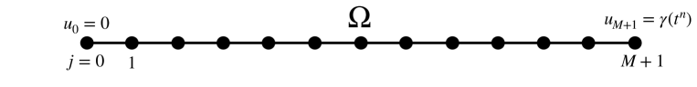
Figure 2: Monodomain grid with $M=11$.

Since we are interested in the stability analysis of the unsteady diffusion equation, we first introduce our spatial and temporal discretization in the context of a monodomain grid. Consider the solution $u(x,t)$ for the unsteady diffusion equation

$$u_{t}=\nu u_{xx},\quad x\in[0,1],\quad\nu>0,$$ (4)

with homogeneous boundary condition on the left boundary, $u(0,t)=0$ and a time-dependent inhomogeneous boundary condition on the right boundary, $u(1,t)=\gamma(t^{n})$.

We model the domain with $M+2$ uniformly-spaced grid points (Fig. 2), such that $\Delta x=\frac{1}{M+1}$. For notational purposes, we introduce $u_{j}^{n}$ to represent the solution $u$ at $j$th grid point at time $t^{n}$, $R$ as the standard restriction matrix (5) that casts the solution from the $M+1$ grid points ${\bar{\underline{u}}}^{n}=[u_{1}^{n},u_{2}^{n},\dots u_{M+1}^{n}]^{T}$ to the $M$ degrees of freedom ${\underline{u}}^{n}=[u_{1}^{n},u_{2}^{n},\dots u_{M}^{n}]^{T}$, and ${\bar{\underline{u}}}_{b}^{n}=[0,0,\dots,0,\gamma(t^{n})]^{T}$ as a vector of length $M+1$ with zeros and the inhomogeneous boundary condition $\gamma(t^{n})$. We have omitted $u_{0}^{n}$ from our vectors (${\bar{\underline{u}}}^{n},{\underline{u}}^{n}$, and ${\bar{\underline{u}}}_{b}$) due to the homogeneous boundary condition at $x=0$. The $M\times M+1$ restriction operator $R$ is an identity matrix, with a column of zeros appended to it:

$$R = \begin{bmatrix}1&0&\ddots&\ddots&\ddots&0&0\\ 0&1&\ddots&\ddots&\ddots&0&0\\ \ddots&\ddots&\ddots&\ddots&\ddots&0&0\\ \ddots&\ddots&\ddots&\ddots&\ddots&0&0\\ \ddots&\ddots&\ddots&\ddots&\ddots&0&0\\ 0&\ddots&\ddots&\ddots&\ddots&1&0\\ \end{bmatrix}.$$ (5)

We use the standard 2nd-order accurate central finite difference operator for $u_{xx}$ that is of size $M+1\times M+1$, and is defined as $\bar{A}_{ii}=2/\Delta x^{2}$ and $\bar{A}_{i-1,i}=\bar{A}_{i+1,i}=-1/\Delta x^{2}$, i.e.,

$$\bar{A} = \frac{1}{\Delta x^{2}}\begin{bmatrix}2&-1&\ddots&\ddots&\ddots&0\\ -1&2&-1&\ddots&\ddots&0\\ \ddots&\ddots&\ddots&\ddots&\ddots&0\\ \ddots&\ddots&\ddots&\ddots&\ddots&0\\ \ddots&\ddots&\ddots&\ddots&\ddots&-1\\ 0&\ddots&\ddots&\ddots&-1&2\\ \end{bmatrix}.$$ (6)

Using a $k$th-order accurate BDF$k$ scheme for discretizing $u_{t}$, it is straightforward to show that the solution of the unsteady heat equation is time-advanced from $t^{n-1}$ to $t^{n}$ at the degrees of freedoms as

$${\underline{u}}^{n}=-\sum_{l=1}^{k}\beta_{l}H^{-1}{\underline{u}}^{n-l}-\nu\Delta tH^{-1}R\bar{A}{\bar{\underline{u}}}_{b}^{n},$$ (7)

where $\Delta t$ is the timestep size (assumed to be the same at all timesteps), $\beta_{l}$ is the coefficient for the BDF$k$ scheme, $H=\beta_{0}I+\nu\Delta tA$ is the Helmholtz matrix, $I$ is a $M\times M$ identity matrix, and $A=R\bar{A}R^{T}$. The system in (7) also depends on the time-dependent inhomogeneous boundary condition, $\gamma(t^{n})$.

3 Unsteady heat equation in overlapping grids

Figure 3: Overlapping grids with $N=7$ and $K=4$.

For solving the unsteady diffusion equation with overlapping grids, we split the monodomain grid ($\Omega$) into two grids ($\Omega^{1}$ and $\Omega^{2}$) with equal number of grid points ($N+2$) and overlap width $K\Delta x$, such that the grid points in the overlap $\Omega^{1}\cap\Omega^{2}$ coincide. Note that we use coincident grids because our focus is the temporal discretization of the method and not the interpolation of interdomain boundary data.

Figure 3 shows the overlapping grids obtained from the monodomain grid of Fig. 2, which are setup such that $M=2N-K+1$. Algebraically, this decomposition is realized through restriction matrices, $R_{i}$ that extract $N$ of the $M$ values from a given vector ${\underline{u}}$ on $\Omega$ as ${\underline{u}}^{i}=R_{i}{\underline{u}}$:

$$R_{1}=\overbrace{\left[\begin{array}[]{ccccccccc}1&0&\ddots&\ddots&\ddots&0&0&\dots&0\\ 0&1&\ddots&\ddots&\ddots&0&0&\dots&0\\ \ddots&\ddots&\ddots&\ddots&\ddots&0&0&\dots&0\\ \ddots&\ddots&\ddots&\ddots&\ddots&0&0&\dots&0\\ \ddots&\ddots&\ddots&\ddots&\ddots&0&0&\dots&0\\ 0&\ddots&\ddots&\ddots&\ddots&1&0&\dots&0\end{array}\right]}^{M},\qquad R_{2}=\overbrace{\left[\begin{array}[]{ccccccccc}0&\dots&0&1&0&\ddots&\ddots&\ddots&0\\ 0&\dots&0&0&1&\ddots&\ddots&\ddots&0\\ 0&\dots&0&\ddots&\ddots&\ddots&\ddots&\ddots&0\\ 0&\dots&0&\ddots&\ddots&\ddots&\ddots&\ddots&0\\ 0&\dots&0&\ddots&\ddots&\ddots&\ddots&\ddots&0\\ 0&\dots&0&0&\ddots&\ddots&\ddots&\ddots&1\end{array}\right]}^{M}.$$ (20)

$$\underset{N}{\underbrace{\rule{142.26378pt}{0.0pt}}}\underset{M-N}{\underbrace{\rule{62.59596pt}{0.0pt}}}\hskip 68.28644pt\underset{M-N}{\underbrace{\rule{59.75095pt}{0.0pt}}}\underset{N}{\underbrace{\rule{139.41832pt}{0.0pt}}}$$

For simplicity, we impose homogeneous boundary conditions at the left boundary of $\Omega^{1}$ ($u^{1,n}_{0}=0$) and right boundary of $\Omega^{2}$ ($u^{2,n}_{N+1}=0$). Here, we have used ${\underline{u}}^{s}$ to represent the solution at the $N$ degrees of freedom of $\Omega^{s}$, and $u^{s,n}_{j}$ to represent the solution at $j$th grid point of $\Omega^{s}$ at $t^{n}$. The homogeneous boundary conditions on $\partial\Omega\backslash\partial\Omega^{s}_{I}$ allow us to use the method developed for the monodomain grid (7), with the difference that the boundary data for the interdomain boundary grid points ($u^{1}_{N+1}$ and $u^{2}_{0}$) is obtained from the corresponding overlapping grid in each subdomain. To effect this interdomain exchange, we define an interpolation operator, $B_{ij}=(I-R_{i}^{T}R_{i})R_{j}^{T}$, that extracts the value from $\Omega^{j}$ at $\partial\Omega^{i}_{I}\cap\Omega^{j}$ and maps it to $\Omega^{i}$. The operator $B_{ij}$ serves the same purpose as the high-order interpolation functionality provided by findpts in the Schwarz-SEM framework for interpolating the interdomain boundary data [32].

3.1 Singlerate timestepping

The singlerate timestepping scheme described in this section was originally developed and analyzed by Peet and Fischer [26], and has shown shown to preserve the temporal convergence of the Schwarz-SEM framework for the incompressible Navier-Stokes equations [1]. In singlerate timestepping, we use the same timestep size $\Delta t$ across all overlapping subdomains to integrate the PDE of interest.

For notational purposes, we introduce ${\underline{u}}^{s,n,q}$ to denote the solution $u$ in $\Omega^{s}$ at the $q$th Schwarz iteration at time $t^{n}$. Thus, assuming that the solution is known up to $t^{n-1}$ and has been converged using $q=1\dots Q$ Schwarz iterations, ${\underline{u}}^{s,n-1,Q}$ denotes the converged solution at $t^{n-1}$. Similar to (7), the solution of the unsteady heat equation is advanced in time by using a BDF$k$ scheme to discretize the time-derivative and replacing the fixed inhomogeneous boundary condition for the monodomain case with the interpolated interdomain boundary data for the overlapping grids. Since the solution is only known up to $t^{n-1}$, the initial Schwarz iterate ($q=0$, the predictor step) uses interdomain boundary data based on $m$th-order extrapolation in time from the solution at previous timesteps in the overlapping subdomain. The $Q$ subsequent Schwarz iterations (the corrector steps) directly interpolate the interdomain boundary data from the most recent iteration. Thus, the boundary data for $\partial\Omega^{s}_{I}$ at the predictor and corrector steps is

$$q=0:{\underline{u}}^{i,n,0}|_{\partial\Omega^{i}_{I}} = B_{ij}\sum_{l=1}^{m}{\alpha}_{l}{\underline{u}}^{j,n-l,Q},$$ (21)

$$q=1\dots Q:{\underline{u}}^{i,n,q}|_{\partial\Omega^{i}_{I}} = B_{ij}{\underline{u}}^{j,n,q-1},$$ (22)

where ${\alpha}_{l}$ are coefficients for the EXT$m$ scheme and $B_{ij}$ is the interpolation operator. Using (21)-(22), the PC approach for solving the unsteady heat equation in overlapping subdomains is

$$q=0:{\underline{u}}^{i,n,0} = -\sum_{l=1}^{k}\beta_{l}H_{i}^{-1}{{\underline{u}}^{i,n-l,Q}}+\sum_{l=1}^{m}{\alpha}_{l}H_{i}^{-1}J_{ij}{\underline{u}}^{j,n-l,Q},$$ (23)

$$q=1\dots Q:\!{\underline{u}}^{i,n,q} = -\sum_{l=1}^{k}\beta_{l}H_{i}^{-1}{{\underline{u}}^{i,n-l,Q}}+H_{i}^{-1}J_{ij}{\underline{u}}^{j,n,q-1},$$ (24)

where

$$\!H_{i}=\beta_{0}I_{i}+\nu\Delta tA_{i},\quad J_{ij}=-\nu\Delta tR_{i}AB_{ij},\quad A_{i}=R_{i}AR_{i}^{T}.$$ (25)

All the matrices in (25) are of size $N\times N$ except the restriction operator $R_{i}$ (20). In Section 4, we analyze the stability of this singlerate timestepping scheme (23)-(24) using the matrix method for stability analysis.

We note that the BDF$k$/EXT$m$ scheme in (23)-(24) will be $k$th-order even if $m=1$, provided that sufficient corrector iterations are done. By using $m$th order extrapolation at the predictor step, we significantly reduce $Q$. Numerical experiments in the Schwarz-SEM framework show that a BDF3/EXT$1$ scheme can take as many as 50 corrector iterations at each time step to achieve third-order temporal convergence. In contrast, a BDF3/EXT3 typically requires only 3-5 corrector iterations.

3.2 Multirate timestepping for the unsteady heat equation in overlapping grids

In [17], we extended the singlerate timestepping scheme described in the previous section to support an arbitrary timestep ratio in an arbitrary number of overlapping subdomains for the incompressible Navier-Stokes equations. This novel multirate timestepping scheme is parallel-in-space and allows each subdomain to integrate the PDE with a time-step based on the local Courant–Friedrichs–Lewy (CFL) number of its mesh. We have demonstrated that the MTS maintains the temporal accuracy of the underlying BDFk/EXTk-based timestepper and accurately models complex turbulent flow and heat transfer phenomenon even when the timestep ratio is as high as 50. Here, we use the MTS scheme developed for the Schwarz-SEM framework to solve the unsteady heat equation in overlapping grids and analyze it using the matrix method for stability analysis.

For MTS, we consider only integer timestep ratios,

$$\eta:=\frac{\Delta t_{c}}{\Delta t_{f}}\in\mathbb{Z}^{+},$$ (26)

where $\Delta t_{c}$ corresponds to the subdomain ($\Omega^{c}$) with larger/coarser time-scales and $\Delta t_{f}$ corresponds to the subdomain ($\Omega^{f}$) with smaller/faster time-scales. Figure 4 shows a schematic of the discrete time-levels for the MTS scheme with an arbitrary timestep ratio. Here, the black circles ($\CIRCLE$) indicate the timestep levels for both $\Omega^{f}$ and $\Omega^{c}$ and the blue circles ( ) indicate the sub-timestep levels for $\Omega^{f}$.

$\begin{array}[]{c}\includegraphics[width=284.52756pt]{figures/mts_arbitrary_scheme}\end{array}$

Figure 4: Schematic showing discrete time-levels for the multirate timestepping with an arbitrary timestep ratio.

Due to the difference in the timestep size, $\Omega^{f}$ has $\eta$ sub-timesteps and $\Omega^{c}$ has a single timestep to integrate the solution from $t^{n-1}$ to $t^{n}$. Similar to the singlerate timestepping scheme, high-order temporal accuracy is achieved in the multirate setting by extrapolating the interdomain boundary data obtained from the solution at previous (sub-) timesteps. For the predictor step, the interdomain boundary data dependency is shown in Fig. 5(left):

$$i=1:{\underline{u}}^{c,n,0}\rvert_{\partial\Omega^{c}_{I}} = B_{cf}\bigg{(}\sum_{j=1}^{m}{\alpha}_{1j}\,{\underline{u}}^{f,n-1-\frac{j-1}{\eta},Q}\bigg{)}.$$ (27)

$$i=1\dots\eta:{\underline{u}}^{f,n-1+\frac{i}{\eta},0}\rvert_{\partial\Omega^{f}_{I}} = B_{fc}\bigg{(}\sum_{j=1}^{m}{\alpha}_{ij}\,{\underline{u}}^{c,n-j,Q}\bigg{)}.$$ (28)

Note that the extrapolation coefficients ${\alpha}_{ij}$ required for extrapolating the interdomain boundary data for each sub-timestep $\Omega^{f}$ are determined using the routines described in [33].

$\begin{array}[]{cc}\includegraphics[width=199.16928pt]{figures/multipredeta}&\includegraphics[width=199.16928pt]{figures/multicoreta}\end{array}$

Figure 5: Schematic showing the dependence of the interdomain boundary data for the (left) predictor and (right) corrector iterations for an arbitrary timestep ratio.

After the predictor iteration, $Q$ corrector iterations are done where the solution in $\Omega^{f}$ is obtained from $\Omega^{c}$ using the converged solution at previous timesteps (${\underline{u}}^{c,n-1,Q}$ and ${\underline{u}}^{c,n-2,Q}$) and the solution from the most recent iteration at the current timestep (${\underline{u}}^{c,n,q-1}$). For the only timestep of $\Omega^{c}$, the solution is directly interpolated from the most recent iteration (${\underline{u}}^{f,n,q-1}$). The interdomain boundary data dependency for the $q=1\dots Q$ corrector iterations is shown in Fig. 5(right):

$$i=1:{\underline{u}}^{c,n,q}\rvert_{\partial\Omega^{c}_{I}} = B_{cf}{\underline{u}}^{f,n,q-1},$$ (29)

$$i=1\dots\eta:{\underline{u}}^{f,n-1+\frac{i}{\eta},q}\rvert_{\partial\Omega^{f}_{I}} = B_{fc}\bigg{(}{\gamma}_{i1}{\underline{u}}^{c,n,q-1}+{\gamma}_{i2}{\underline{u}}^{c,n-1,Q}+{\gamma}_{i3}{\underline{u}}^{c,n-2,Q}\bigg{)}.$$ (30)

Note that we compute the interpolation coefficients ${\gamma}_{ij}$ assuming linear interpolation when $m=1$ or $2$, and quadratic interpolation when $m=3$. This approach ensures that the desired temporal accuracy $\mathcal{O}(\Delta t^{m})$ is maintained for the BDF$k$/EXT$m$-based scheme.

Equations (27)-(30) are used to solve the unsteady heat equation with multirate timestepping in two overlapping grids with a formulation similar to (23)-(24). The predictor step ($q=0$) for the only timestep of $\Omega^{c}$ and $\eta$ sub-timesteps of $\Omega^{f}$ is:

$${\underline{u}}^{c,n,0} = -\sum_{l=1}^{k}\beta_{l}H_{c}^{-1}{\underline{u}}^{c,n-l,Q}+\sum_{l=1}^{m}{\alpha}_{l}H_{c}^{-1}J_{cf}{\underline{u}}^{f,n-1-\frac{l-1}{\eta},Q},$$ (31)

$$i=1\dots\eta:{\underline{u}}^{f,n-1+\frac{i}{\eta},0} = -\sum_{l=1}^{k}\beta_{l}H_{f}^{-1}{\underline{u}}^{f,n-1+\frac{i-l}{\eta},Q}+\sum_{l=1}^{m}{\alpha}_{il}H_{f}^{-1}J_{fc}{\underline{u}}^{c,n-l,Q},$$ (32)

and the $Q$ corrector iterations are

$${\underline{u}}^{c,n,q} = -\sum_{l=1}^{k}\beta_{l}H_{c}^{-1}{\underline{u}}^{c,n-l,Q}+H_{c}^{-1}J_{cf}{\underline{u}}^{f,n,q-1},$$ (33)

$$i=1\dots\eta:{\underline{u}}^{f,n-1+\frac{i}{\eta},q} = -\sum_{l=1}^{k}\beta_{l}H_{f}^{-1}{\underline{u}}^{f,n-1+\frac{i-l}{\eta},Q}$$

$$+H_{f}^{-1}J_{fc}\bigg{(}{\gamma}_{i1}{\underline{u}}^{c,n,q-1}+{\gamma}_{i2}{\underline{u}}^{c,n-1,Q}+{\gamma}_{i3}{\underline{u}}^{c,n-2,Q}\bigg{)}.$$

The $H$ and $J$ operators used here for multirate timestepping are similar to the operators of singlerate timestepping (25), with the only difference that the timestep size used in their construction is different for each subdomain.

We analyze the stability of the multirate timestepping scheme described here (31)-(3.2) in Section 5 using the matrix method for stability analysis.

4 Stability of singlerate PC method

In this section, we analyze the stability of the singlerate PC scheme by casting it as ${\underline{z}}^{n}=G{\underline{z}}^{n-1}$, where $G=C^{Q}P$ is a product of the matrix $P$ corresponding to the predictor step with the EXT$m$ scheme (23) and matrix $C$ corresponding to the $Q$ corrector steps (24).

Introducing the notation ${\underline{z}}^{n,q}$ to denote the vector of solutions in both overlapping subdomains

$${\underline{z}}^{n,q}=\big{[}{\underline{u}}^{1,n,q^{T}}\,{\underline{u}}^{2,n,q^{T}}\,{\underline{u}}^{1,n-1,Q^{T}}\,{\underline{u}}^{2,n-1,Q^{T}}\,{\underline{u}}^{1,n-2,Q^{T}}\,{\underline{u}}^{2,n-2,Q^{T}}\,{\underline{u}}^{1,n-3,Q^{T}}\,{\underline{u}}^{2,n-3,Q^{T}}\big{]}^{T},$$ (35)

the predictor step (23) is

$$\underbrace{\left[\begin{array}[]{c}{\underline{u}}^{1,n,0}\\ {\underline{u}}^{2,n,0}\\ {\underline{u}}^{1,n-1,Q}\\ {\underline{u}}^{2,n-1,Q}\\ {\underline{u}}^{1,n-2,Q}\\ {\underline{u}}^{2,n-2,Q}\\ {\underline{u}}^{1,n-3,Q}\\ {\underline{u}}^{2,n-3,Q}\\ \end{array}\right]}_{\begin{subarray}{c}{\underline{z}}^{n,0}\end{subarray}}=\underbrace{\begin{pmatrix}-\beta_{1}{H_{1}^{-1}}&{\alpha}_{1}{H_{1}^{-1}}J_{12}&-\beta_{2}{H_{1}^{-1}}&{\alpha}_{2}{H_{1}^{-1}}J_{12}&-\beta_{3}{H_{1}^{-1}}&{\alpha}_{3}{H_{1}^{-1}}J_{12}&0&0\\ {\alpha}_{1}{H_{2}^{-1}}J_{21}&-\beta_{1}{H_{2}^{-1}}&{\alpha}_{2}{H_{2}^{-1}}J_{21}&-\beta_{2}{H_{2}^{-1}}&{\alpha}_{3}{H_{2}^{-1}}J_{21}&-\beta_{3}{H_{2}^{-1}}&0&0\\ I_{1}&0&0&0&0&0&0&0\\ 0&I_{2}&0&0&0&0&0&0\\ 0&0&I_{1}&0&0&0&0&0\\ 0&0&0&I_{2}&0&0&0&0\\ 0&0&0&0&I_{1}&0&0&0\\ 0&0&0&0&0&I_{2}&0&0\\ \end{pmatrix}}_{\begin{subarray}{c}P\end{subarray}}\underbrace{\left[\begin{array}[]{c}{\underline{u}}^{1,n-1,Q}\\ {\underline{u}}^{2,n-1,Q}\\ {\underline{u}}^{1,n-2,Q}\\ {\underline{u}}^{2,n-2,Q}\\ {\underline{u}}^{1,n-3,Q}\\ {\underline{u}}^{2,n-3,Q}\\ {\underline{u}}^{1,n-4,Q}\\ {\underline{u}}^{2,n-4,Q}\end{array}\right]}_{\begin{subarray}{c}{\underline{z}}^{n-1,Q}\end{subarray}}$$ (52)

where the interdomain boundary data is extrapolated from the previous timesteps in the overlapping subdomain. Similarly, the matrix $C$ corresponding to the $Q$ corrector iterations from (24) is given by (69) where the solution $z^{n,q}$ depends on the interdomain boundary data interpolated from the most recent Schwarz iteration ($z^{n,q-1}$). Using (52) and (69), the solution is advanced in time as $z^{n,Q}=Gz^{n-1,Q}$, $G=C^{Q}P$, and the spectral radius of $G$ is used to determine the stability of the PC scheme for different grid sizes, overlap widths, extrapolation orders, and corrector iterations. We note that using the parameters $N$ and $K$, the grid overlap width is determined as $K\Delta x=K/(2N-K+2)$.

$$\underbrace{\left[\begin{array}[]{c}{\underline{u}}^{1,n,q}\\ {\underline{u}}^{2,n,q}\\ {\underline{u}}^{1,n-1,Q}\\ {\underline{u}}^{2,n-1,Q}\\ {\underline{u}}^{1,n-2,Q}\\ {\underline{u}}^{2,n-2,Q}\\ {\underline{u}}^{1,n-3,Q}\\ {\underline{u}}^{2,n-3,Q}\\ \end{array}\right]}_{\begin{subarray}{c}{\underline{z}}^{n,q}\end{subarray}}=\underbrace{\begin{pmatrix}0&{H_{1}^{-1}}J_{12}&-\beta_{1}{H_{1}^{-1}}&0&-\beta_{2}{H_{1}^{-1}}&0&-\beta_{3}{H_{1}^{-1}}&0\\ {H_{2}^{-1}}J_{21}&0&0&-\beta_{1}{H_{2}^{-1}}&0&-\beta_{2}{H_{2}^{-1}}&0&-\beta_{3}{H_{2}^{-1}}\\ 0&0&I_{1}&0&0&0&0&0\\ 0&0&0&I_{2}&0&0&0&0\\ 0&0&0&0&I_{1}&0&0&0\\ 0&0&0&0&0&I_{2}&0&0\\ 0&0&0&0&0&0&I_{1}&0\\ 0&0&0&0&0&0&0&I_{2}\\ \end{pmatrix}}_{\begin{subarray}{c}C\end{subarray}}\underbrace{\left[\begin{array}[]{c}{\underline{u}}^{1,n,q-1}\\ {\underline{u}}^{2,n,q-1}\\ {\underline{u}}^{1,n-1,Q}\\ {\underline{u}}^{2,n-1,Q}\\ {\underline{u}}^{1,n-2,Q}\\ {\underline{u}}^{2,n-2,Q}\\ {\underline{u}}^{1,n-3,Q}\\ {\underline{u}}^{2,n-3,Q}\\ \end{array}\right]}_{\begin{subarray}{c}{\underline{z}}^{n,q-1}\end{subarray}}$$ (69)

4.1 Stability Results for different BDF$k$/EXT$m$ schemes

In this section, we look at the stability of different BDF$k$/EXT$m$ schemes with $Q$. We set $N=32$ and $K=5$, and in each case, we vary the nondimensional timestep size ($\nu\Delta t/\Delta x^{2}$) to see how the spectral radius of the propogation operator changes.

Figure 6 shows the spectral radius for the BDF$k$/EXT$m$ schemes for $k=1\dots 3$ and $m\leq k$. We observe that the BDF$k$/EXT$1$ schemes are unconditionally stable, and the use of high-order extrapolation ($m>1$) for interdomain boundary data requires correct iterations for stability. These results are also indicated in [26]. A novel result that comes forth from Fig. 6 is that for high-order extrapolation, i.e., BDF$k$/EXT$2$ and BDF$k$/EXT$3$ schemes, odd $Q$ is relatively more stable than even $Q$. To the best of our knowledge, this behavior has not been observed in the current literature for overlapping grids. In terms of general ODEs and PDEs for a single domain, there is a sparse evidence of such behavior. We will discuss this in the context of existing literature and connect it to the Schwarz-SEM framework for INSE in Section 4.2.

$\begin{array}[]{ccc}\includegraphics[height=113.81102pt]{figures/rho_vs_s_n132_k5_BDF1_EXT1}&\includegraphics[height=113.81102pt]{figures/rho_vs_s_n132_k5_BDF2_EXT1}&\includegraphics[height=113.81102pt]{figures/rho_vs_s_n132_k5_BDF2_EXT2}\\ \textrm{(a) BDF$1$/EXT$1$}&\textrm{(b) BDF$2$/EXT$1$}&\textrm{(c) BDF$2$/EXT$2$}\\ \includegraphics[height=113.81102pt]{figures/rho_vs_s_n132_k5_BDF3_EXT1}&\includegraphics[height=113.81102pt]{figures/rho_vs_s_n132_k5_BDF3_EXT2}&\includegraphics[height=113.81102pt]{figures/rho_vs_s_n132_k5_BDF3_EXT3}\\ \textrm{(d) BDF$3$/EXT$1$}&\textrm{(e) BDF$3$/EXT$2$}&\textrm{(f) BDF$3$/EXT$3$}\\ \lx@intercol\hfil\includegraphics[width=426.79134pt]{figures/legend}\hfil\lx@intercol\\ \end{array}$

Figure 6: Spectral radius $\rho(G)$ versus nondimensional time $\frac{\nu\Delta t}{\Delta x^{2}}$ for different BDF$k$/EXT$m$ schemes with $Q=0\dots 7$, $N=32$ and $K=5$.

4.1.1 Effect of increasing subdomain overlap

The subdomain overlap width has an impact on the convergence of Schwarz-based methods [34]. For practical purposes, one would like to minimize the overlap width to minimize the total number of elements needed for modeling a domain. Thus, we look at the impact of overlap width on the stability of the PC scheme. Since we are mainly interested in the high-order extrapolation scheme ($m=1$ is unconditionally stable as shown in the previous section), we look at the results for the BDF2/EXT2, BDF3/EXT2, and BDF3/EXT3 schemes, with $N=32$, and change the grid overlap parameter, $K$.

Figure 7 show that increasing the overlap width increases the stability range over which a given scheme is stable for a specified number of corrector iterations $Q$. We also notice that high-order extrapolation schemes are less stable as compared to their low order counterparts, e.g., the BDF3/EXT3 scheme is less stable than the BDF3/EXT2 scheme, for a given $Q$.

$\begin{array}[]{ccc}\includegraphics[height=113.81102pt]{figures/rho_vs_s_n132_k3_BDF2_EXT2}&\includegraphics[height=113.81102pt]{figures/rho_vs_s_n132_k5_BDF2_EXT2}&\includegraphics[height=113.81102pt]{figures/rho_vs_s_n132_k7_BDF2_EXT2}\\ \lx@intercol\hfil\textrm{(a) BDF2/EXT2}\hfil\lx@intercol\\ \includegraphics[height=113.81102pt]{figures/rho_vs_s_n132_k3_BDF3_EXT2}&\includegraphics[height=113.81102pt]{figures/rho_vs_s_n132_k5_BDF3_EXT2}&\includegraphics[height=113.81102pt]{figures/rho_vs_s_n132_k7_BDF3_EXT2}\\ \lx@intercol\hfil\textrm{(b) BDF3/EXT2}\hfil\lx@intercol\\ \includegraphics[height=113.81102pt]{figures/rho_vs_s_n132_k3_BDF3_EXT3}&\includegraphics[height=113.81102pt]{figures/rho_vs_s_n132_k5_BDF3_EXT3}&\includegraphics[height=113.81102pt]{figures/rho_vs_s_n132_k7_BDF3_EXT3}\\ \lx@intercol\hfil\textrm{(c) BDF3/EXT3}\hfil\lx@intercol\\ \textrm{(i) $N=32,K=3$}&\textrm{(ii) $N=32,K=5$}&\textrm{(iii) $N=32,K=7$}\\ \lx@intercol\hfil\includegraphics[width=398.33858pt]{figures/legend}\hfil\lx@intercol\\ \end{array}$

Figure 7: Spectral radius $\rho(G)$ versus nondimensional time $\frac{\nu\Delta t}{\Delta x^{2}}$ for (a) BDF2/EXT2, (b) BDF3/EXT2, and (c) BDF3/EXT3 scheme with $N=32$ and varying $K$: (left to right) (i) $K=3$, (ii) $K=5$, and (iii) $K=7$.

4.1.2 Effect of increasing grid resolution while keeping overlap fixed

For certain applications (e.g, Fig. 1.1 of [35]), geometric constraints can limit the maximum allowable overlap width between different subdomains. In these cases, if the overlap width is not enough for a stable predictor-corrector scheme with $m>1$, the application of the Schwarz-SEM framework is limited. Thus, we look at the impact of increasing the grid resolution, while keeping the overlap width fixed in Fig. 8. These results show that increasing the grid resolution has a stabilizing effect on the PC scheme.

$\begin{array}[]{ccc}\includegraphics[height=113.81102pt]{figures/rho_vs_s_n132_k5_BDF2_EXT2}&\includegraphics[height=113.81102pt]{figures/rho_vs_s_n165_k10_BDF2_EXT2}&\includegraphics[height=113.81102pt]{figures/rho_vs_s_n198_k15_BDF2_EXT2}\\ \lx@intercol\hfil\textrm{(a) BDF2/EXT2}\hfil\lx@intercol\\ \includegraphics[height=113.81102pt]{figures/rho_vs_s_n132_k5_BDF3_EXT2}&\includegraphics[height=113.81102pt]{figures/rho_vs_s_n165_k10_BDF3_EXT2}&\includegraphics[height=113.81102pt]{figures/rho_vs_s_n198_k15_BDF3_EXT2}\\ \lx@intercol\hfil\textrm{(b) BDF3/EXT2}\hfil\lx@intercol\\ \includegraphics[height=113.81102pt]{figures/rho_vs_s_n132_k5_BDF3_EXT3}&\includegraphics[height=113.81102pt]{figures/rho_vs_s_n165_k10_BDF3_EXT3}&\includegraphics[height=113.81102pt]{figures/rho_vs_s_n198_k15_BDF3_EXT3}\\ \lx@intercol\hfil\textrm{(c) BDF3/EXT3}\hfil\lx@intercol\\ \textrm{(i) $N=32,K=5$}&\textrm{(ii) $N=65,K=10$}&\textrm{(iii) $N=98,K=15$}\\ \lx@intercol\hfil\includegraphics[width=398.33858pt]{figures/legend}\hfil\lx@intercol\\ \end{array}$

Figure 8: Spectral radius $\rho(G)$ versus nondimensional time $\frac{\nu\Delta t}{\Delta x^{2}}$ for (a) BDF2/EXT2, (b) BDF3/EXT2, and (c) BDF3/EXT3 scheme with $N$ and $K$ varying such that $K\Delta x$ is fixed: (left to right) (i) $N=32$, $K=5$, (ii) $N=65$, $K=10$, and (iii) $N=98$, $K=15$.

4.2 Difference between stability behavior for odd and even $Q$

Figure 6 shows that for the high-order BDF$k$/EXT$m$ scheme used in the Schwarz-SEM framework, odd-$Q$ leads to a relatively more stable formulation than even-$Q$. Love et al. have described similar behavior for a second-order predictor-corrector scheme using a FD-based staggered grid formulation for Lagrangian shock hydrodynamics [29]. Similarly, Stetter’s stability analysis of a high-order Adam Bashforth- (AB3) and Adam Moulton-based (AM2) predictor-corrector scheme for ODEs shows a difference in the stability of odd- and even-$Q$, although this is not a part of Stetter’s discussion.

$\begin{array}[]{c}\includegraphics[height=213.39566pt]{figures/ab3am2stability.jpeg}\end{array}$

Figure 9: Stability diagram for the AB3/AM2 predictor-corrector scheme for different number of corrector iterations. The curve corresponding to each $Q$ is labelled where it intersects with the horizontal-axis to show that the PC scheme is more stable for odd-$Q$.

Figure 9 shows the stability diagram for the AB3/AM2-based PC scheme used to solve $\frac{du}{dt}=\lambda u$ by Stetter. We observe that when $\lambda$ is real-valued, the timestepping scheme is relatively more stable for odd-$Q$ as compared to the even-$Q$. These stability results for the AB3/AM2-based scheme are similar to the results of the high-order predictor-corrector scheme in our work because we solve the unsteady heat equation, where the diffusion operator has negative real eigenvalues. We have also found that stability analysis of a BDF$k$/EXT$m$-based scheme for $\frac{du}{dt}=\lambda u$ shows a similar behavior for odd- and even-$Q$. Finally, this behavior is also evident in the Schwarz-SEM framework where the PC scheme is applied to the INSE with the diffusion order replaced by the unsteady Stokes operator [21].

4.2.1 Stability with $Q$ in the Schwarz-SEM framework

The odd-even pattern that we have observed in the Schwarz-SEM framework is straightforward to demonstrate by considering the exact Navier-Stokes eigenfunctions by Walsh [36], in a periodic domain $\Omega=[0,2\pi]^{2}$.

Walsh introduced families of eigenfunctions that can be defined using linear combinations of $\cos(px)\cos(qy),$ $\sin(px)\cos(qy),$ $\cos(px)\sin(qy),$ and $\sin(px)\sin(qy)$, for all integer pairs ($p,q$) satisfying $\lambda=-(p^{2}+q^{2})$. Taking as an initial condition the eigenfunction $\hat{{\bf u}}=(-{\psi}_{y},{\psi}_{x})$, a solution to the NSE is ${\bf u}=e^{\nu\lambda t}\hat{{\bf u}}({\bf x})$. Here, ${\psi}$ is the streamfunction resulting from the linear combinations of eigenfunctions. Interesting long-time solutions can be realized by adding a relatively high-speed mean flow ${\bf u}_{0}$ to the eigenfunction, in which case the solution is ${\bf u}_{exact}=e^{\nu\lambda t}\hat{{\bf u}}[{\bf x}-{\bf u}_{0}t]$, where the brackets imply that the argument is modulo $2\pi$ in $x$ and $y$.

In the Schwarz-SEM framework, we model this periodic domain using two overlapping meshes such that the periodic background mesh with a hole in its center has 240 elements, which is covered with a circular mesh with 96 elements, as shown in Fig. 10(a). The flow parameters are $\nu=0.05$, ${\bf u}_{0}=(1,0.3)$, ${\psi}=(1/5)sin(5y)+(1/5)cos(5x)-(1/4)sin(3x)sin(4y)$, and $\lambda=-25$. The flow is integrated up to time $T=1$ convective time units (CTU) with a fixed $\Delta t=2\times 10^{-4}$. The polynomial order for representing the solution is set to $N=7$. Figure 10(b) shows the vorticity contours for the solution at $T_{f}=1$ with $\Delta t=2\times 10^{-4}$.

Since the exact solution is known, we compute the error in time as $||{{\underline{\bf e}}}||_{2,\infty}$, where ${\underline{\bf e}}={\underline{\bf u}}-{\underline{\bf u}}_{exact}$ and the norm is the 2-norm of the point-wise maximum of the vector field. Figure 10(c) shows the error in solution versus time for different $Q$, and as evident, the solution is stable for $Q=1$ and 3 but unstable for $Q=2$ and 4. We have also observed similar behavior for odd- and even-$Q$ in highly turbulent flow calculations using the Schwarz-SEM framework.

$\begin{array}[]{ccc}\includegraphics[height=128.0374pt]{figures/eddy_nn_grid_ov}&\includegraphics[height=128.0374pt]{figures/eddy_vort}&\includegraphics[height=128.0374pt]{figures/eddyoddeven}\end{array}$

Figure 10: (left to right) (a) Spectral element mesh for each overlapping subdomain. The background mesh has 240 elements and is covered by a circular mesh with 96 elements. (b) Vorticity contours at $T_{f}=1$ with $N=7$ and $Q=3$. (c) Error variation for the Navier-Stokes eigenfunctions test case with different $Q$ using $\Delta t=2\times 10^{-3}$ and $N=7$.

Based on the stability analyses presented in this section and the numerical experiments that we have done with the Schwarz-SEM framework, we conjecture that for BVP (dominated) with negative real eigenvalues, high-order PC schemes lead to a difference in the stability between odd- and even-corrector iterations. In future work, we will continue this work to determine the fundamental reasoning behind this odd-even pattern, and look at the stability of high-order PC methods for general boundary value problems, including the unsteady Stokes problem in our SEM-based framework.

4.3 Improving the Stability for Even-Corrector Iterations

In the predictor-corrector scheme discussed so far, since odd-$Q$ is more stable than even-$Q$, we have to increase $Q$ by 2 (e.g., increase $Q=1$ to $Q=3$) if the number of corrector iterations is not sufficient from a stability standpoint. Since each corrector iteration requires an additional PDE solve and thus increases the computational cost the calculation, we modify our PC scheme to improve the stability for even-$Q$.

In [30], Stetter improves the stability of the AB3/AM2 PC scheme by using a linear combination of solution from each corrector iteration to determine the final solution as

$$u^{n} = \sum_{q=0}^{Q}\gamma_{q}u^{n,q},\qquad\sum_{q=0}^{Q}\gamma_{q}=1,$$ (70)

where $\gamma_{q}$ is some weight corresponding to the solution of $q$th iterate at each timestep. Using this approach, Stetter shows that the stability region for the PC scheme can be extended for any $\lambda$. Since we are primarily concerned with the inferior stability properties of even-$Q$, we extend Stetter’s idea to modify only the last corrector iteration when $Q$ is even.

The proposed predictor-corrector scheme is

$$q=0:\!{\underline{u}}_{i}^{n,0} = -\sum_{l=1}^{k}\beta_{l}H_{i}^{-1}{{\underline{u}}^{i,n-l}}+\sum_{l=1}^{m}{\alpha}_{l}H_{i}^{-1}J_{ij}{\underline{u}}_{j}^{n-l},$$ (71)

$$q=1\dots Q-1:\!{\underline{u}}_{i}^{n,q} = -\sum_{l=1}^{k}\beta_{l}H_{i}^{-1}{{\underline{u}}^{i,n-l}}+H_{i}^{-1}J_{ij}{\underline{u}}_{j}^{n,q-1},$$ (72)

$$q=Q:\!{\underline{u}}_{i}^{n,q} = -\sum_{l=1}^{k}\beta_{l}H_{i}^{-1}{{\underline{u}}^{i,n-l}}+H_{i}^{-1}J_{ij}\bigg{(}\gamma{\underline{u}}_{j}^{n,Q-1}+(1-\gamma){\underline{u}}_{j}^{n,Q-2}\bigg{)},$$ (73)

where $\gamma$ is a parameter that uses the combination of the two most recent solutions (instead of just the most recent solution) at the last corrector iteration. We set $\gamma=1$ when $Q$ is odd to recover the original PC scheme (23-24), and $0<\gamma<1$ when $Q$ is even. The rationale behind this new predictor-corrector scheme is that we do not want to modify the convergence properties of the original PC scheme if $Q$ is odd. Thus, we modify only the last corrector iteration ($u^{n,Q}$), when $Q$ is even.

Figure 11 shows the stability plot for the modified predictor-corrector schemes for different values of $\gamma$ for $Q=2$, and $Q=3$ with $\gamma=1$. The parameters for grid size are $N=32$ and $K=5$ and we use the BDF3/EXT3 scheme for time-integration. We see that $Q=2,\gamma=1$ leads to the original scheme and $Q=2,\gamma=0$ restores the behavior of the original scheme with $Q=1$. It is also apparent that the stability of the PC scheme has significantly improved for $Q=2$, in comparison to the original scheme (Fig. 6), and it is no longer more unstable than $Q=1$ when $\gamma=0.25$ or 0.5. Figure 12 compares the stability plots for the original and improved predictor-corrector scheme ($\gamma=0.5$ for even-$Q$), and we see that the proposed formulation leads to a scheme with monotonically increasing stability with $Q$.

$\begin{array}[]{c}\includegraphics[height=170.71652pt]{figures/rho_vs_s_n132_k5_BDF3_EXT3_gamma}\end{array}$

Figure 11: Spectral radius $\rho(G)$ versus nondimensional time $\frac{\nu\Delta t}{\Delta x^{2}}$ for the BDF3/EXT3 scheme with $N=32$, $K=5$ for different $\gamma$.

$\begin{array}[]{cc}\includegraphics[height=170.71652pt]{figures/rho_vs_s_n132_k5_BDF3_EXT3}&\includegraphics[height=170.71652pt]{figures/rho_vs_s_n132_k5_BDF3_EXT3_improved}\\ \lx@intercol\hfil\includegraphics[width=426.79134pt]{figures/legend}\hfil\lx@intercol\\ \textrm{(a) Original PC scheme}&\textrm{(b) Improved PC scheme}\end{array}$

Figure 12: Spectral radius $\rho(G)$ versus nondimensional time $\frac{\nu\Delta t}{\Delta x^{2}}$ for the BDF3/EXT3 scheme with $N=32$ and $K=5$ comparing the original and improved predictor-corrector scheme. $\gamma=0.5$ for even-$Q$ in the improved PC scheme.

The improved predictor-corrector scheme for even-$Q$ can be readily extended to the Schwarz-SEM framework. Using the exact Navier-Stokes eigenfunctions, Fig. 13 shows the error variation for $Q=1,2,$ 3 and 4 with the original scheme, and compares it to the improved PC scheme with $Q=2$ and 4 for $\gamma=0.5$. In [35], we have also verified that the improved PC scheme maintains $m$th-order temporal accuracy of the underlying SEM-based solver.

Figure 13: Error variation for the Navier-Stokes eigenfunctions test case from Section 4.2.1 with different $Q$ using $\Delta t=2\times 10^{-3}$ and $N=7$ comparing the original ( ) and improved (   ) predictor-corrector scheme.

5 Stability of multirate PC method

Next, we analyze the multirate PC scheme described in Section 3.2 using the matrix method for stability analysis. For a timestep ratio $\eta$, advancing the solution from $t^{n-1}$ to $t^{n}$ requires the PDE of interest to be solved $\eta$ times in $\Omega^{f}$ and once in $\Omega^{c}$. Thus, casting the multirate timestepping scheme into a system ${\underline{z}}^{n}=G{\underline{z}}^{n-1}$ is not as straightforward as it is for the singlerate scheme. For simplicity, we describe the method to cast the multirate PC scheme (31)-(3.2) for $\eta=2$, and this method readily extends to arbitrary $\eta$.

For notational purposes, we define

$${\underline{z}}^{n}=\big{[}{\underline{u}}^{c,n^{T}}\,{\underline{u}}^{f,n^{T}}\,{\underline{u}}^{f,n-1/2^{T}}\,{\underline{u}}^{c,n-1^{T}}\,{\underline{u}}^{f,n-1^{T}}\,{\underline{u}}^{f,n-3/2^{T}}\,{\underline{u}}^{c,n-2^{T}}\,{\underline{u}}^{f,n-2^{T}}\,{\underline{u}}^{f,n-5/2^{T}}\,{\underline{u}}^{c,n-3^{T}}\,{\underline{u}}^{f,n-3^{T}}\big{]}^{T},$$ (74)

where ${\underline{u}}^{f}$ and ${\underline{u}}^{c}$ are the solution vectors for subdomain $\Omega^{f}$ and $\Omega^{c}$, respectively, and we use ${\underline{z}}^{n,q}$ to represent the vector with solutions at $q$th corrector iteration. To account for the sub-timestep solution for $\Omega^{f}$ in ${\underline{z}}^{n}$, we modify our methodology of building the predictor and corrector matrices. The predictor matrix is now a product of $\eta$ matrices, of which $\eta-1$ matrices correspond to the sub-timesteps of $\Omega^{f}$, and 1 matrix for the last sub-timestep of $\Omega^{f}$ and the only step of $\Omega^{c}$. For $\eta=2$, the predictor matrix is $P=P_{2}P_{1}$ where $P_{1}$ outputs the solution ${\underline{u}}^{f,n-\frac{1}{2},0}$ and $P_{2}$ outputs the solution ${\underline{u}}^{c,n,0}$ and ${\underline{u}}^{f,n,0}$. The matrices $P_{2}$ and $P_{1}$ are

$\left[\begin{array}[]{c}u^{f,n-\frac{1}{2},0}\\ u^{c,n-1,Q}\\ u^{f,n-1,Q}\\ u^{f,n-\frac{3}{2},Q}\\ u^{c,n-2,0}\\ u^{f,n-2,Q}\\ u^{f,n-\frac{5}{2},Q}\\ u^{c,n-3,Q}\\ u^{f,n-3,0}\end{array}\right]=$ $\underbrace{\setcounter{MaxMatrixCols}{11}\begin{pmatrix}{\alpha}_{11}H_{f}^{-1}J_{fc}&-\beta_{1}H_{f}^{-1}&-\beta_{2}H_{f}^{-1}&{\alpha}_{12}H_{f}^{-1}J_{fc}&-\beta_{3}H_{f}^{-1}&0&{\alpha}_{13}H_{f}^{-1}J_{fc}&0&0&0&0\\ I_{1}&0&0&0&0&0&0&0&0&0&0\\ 0&I_{2}&0&0&0&0&0&0&0&0&0\\ 0&0&I_{2}&0&0&0&0&0&0&0&0\\ 0&0&0&I_{1}&0&0&0&0&0&0&0\\ 0&0&0&0&I_{2}&0&0&0&0&0&0\\ 0&0&0&0&0&I_{2}&0&0&0&0&0\\ 0&0&0&0&0&0&I_{1}&0&0&0&0\\ 0&0&0&0&0&0&0&I_{2}&0&0&0\\ \end{pmatrix}}_{P_{1}}$ $\underbrace{\left[\begin{array}[]{c}u^{c,n-1,Q}\\ u^{f,n-1,Q}\\ u^{f,n-\frac{3}{2},Q}\\ u^{c,n-2,Q}\\ u^{f,n-2,Q}\\ u^{f,n-\frac{5}{2},Q}\\ u^{c,n-3,Q}\\ u^{f,n-3,Q}\\ u^{f,n-\frac{7}{2},Q}\\ u^{c,n-4,Q}\\ u^{f,n-4,Q}\end{array}\right]}_{{\underline{z}}^{n,Q}}$,


$\underbrace{\left[\begin{array}[]{c}u^{c,n,0}\\ u^{f,n,0}\\ u^{f,n-\frac{1}{2},0}\\ u^{c,n-1,Q}\\ u^{f,n-1,Q}\\ u^{f,n-\frac{3}{2},Q}\\ u^{c,n-2,Q}\\ u^{f,n-2,Q}\\ u^{f,n-\frac{5}{2},Q}\\ u^{c,n-3,Q}\\ u^{f,n-3,Q}\end{array}\right]}_{{\underline{z}}^{n,0}}=$ $\underbrace{\begin{bmatrix}0&-\beta_{1}H_{c}^{-1}&{\alpha}_{21}H_{c}^{-1}J_{cf}&{\alpha}_{22}H_{c}^{-1}J_{cf}&-\beta_{2}H_{c}^{-1}&{\alpha}_{23}H_{c}^{-1}J_{cf}&0&-\beta_{3}H_{c}^{-1}&0\\ -\beta_{1}H_{f}^{-1}&{\alpha}_{1}H_{f}^{-1}J_{fc}&-\beta_{2}H_{f}^{-1}&-\beta_{3}H_{f}^{-1}&{\alpha}_{2}H_{f}^{-1}J_{fc}&0&0&{\alpha}_{3}H_{f}^{-1}J_{fc}&0\\ I_{2}&0&0&0&0&0&0&0&0\\ 0&I_{1}&0&0&0&0&0&0&0\\ 0&0&I_{2}&0&0&0&0&0&0\\ 0&0&0&I_{2}&0&0&0&0&0\\ 0&0&0&0&I_{1}&0&0&0&0\\ 0&0&0&0&0&I_{2}&0&0&0\\ 0&0&0&0&0&0&I_{2}&0&0\\ 0&0&0&0&0&0&0&I_{1}&0\\ 0&0&0&0&0&0&0&0&I_{2}\\ \end{bmatrix}}_{P_{2}}$ $\left[\begin{array}[]{c}u^{f,n-\frac{1}{2},0}\\ u^{c,n-1,Q}\\ u^{f,n-1,Q}\\ u^{f,n-\frac{3}{2},Q}\\ u^{c,n-2,Q}\\ u^{f,n-2,Q}\\ u^{f,n-\frac{5}{2},Q}\\ u^{c,n-3,Q}\\ u^{f,n-3,Q}\end{array}\right]$. Thus, the predictor step to time-advance the solution in $\Omega^{f}$ and $\Omega^{c}$ from $t^{n-1}$ to $t^{n}$ is ${\underline{z}}^{n,0}=P_{2}P_{1}{\underline{z}}^{n,q}$. Similarly, the system for corrector iterations is

$\left[\begin{array}[]{c}u^{c,n,q-1}\\ u^{f,n,q-1}\\ u^{f,n-\frac{1}{2},q}\\ u^{c,n-1,Q}\\ u^{f,n-1,Q}\\ u^{f,n-\frac{3}{2},Q}\\ u^{c,n-2,Q}\\ u^{f,n-2,Q}\\ u^{f,n-\frac{5}{2},Q}\\ u^{c,n-3,Q}\\ u^{f,n-3,Q}\end{array}\right]=$ $\underbrace{\setcounter{MaxMatrixCols}{12}\begin{bmatrix}I_{1}&0&0&0&0&0&0&0&0&0&0&\\ 0&I_{2}&0&0&0&0&0&0&0&0&0&\\ {\gamma}_{11}H_{f}^{-1}J_{fc}&0&0&{\gamma}_{12}H_{f}^{-1}J_{fc}&-\beta_{1}H_{f}^{-1}&-\beta_{2}H_{f}^{-1}&{\gamma}_{13}H_{f}^{-1}J_{fc}&-\beta_{3}H_{f}^{-1}&0&0&0\\ 0&0&0&I_{1}&0&0&0&0&0&0&0\\ 0&0&0&0&I_{2}&0&0&0&0&0&0\\ 0&0&0&0&0&I_{2}&0&0&0&0&0\\ 0&0&0&0&0&0&I_{1}&0&0&0&0\\ 0&0&0&0&0&0&0&I_{2}&0&0&0\\ 0&0&0&0&0&0&0&0&I_{2}&0&0\\ 0&0&0&0&0&0&0&0&0&I_{1}&0\\ 0&0&0&0&0&0&0&0&0&0&I_{2}\\ \end{bmatrix}}_{C_{1}}$ $\underbrace{\left[\begin{array}[]{c}u^{c,n,q-1}\\ u^{f,n,q-1}\\ u^{f,n-\frac{1}{2},q-1}\\ u^{c,n-1,Q}\\ u^{f,n-1,Q}\\ u^{f,n-\frac{3}{2},Q}\\ u^{c,n-2,Q}\\ u^{f,n-2,Q}\\ u^{f,n-\frac{5}{2},Q}\\ u^{c,n-3,Q}\\ u^{f,n-3,Q}\end{array}\right]}_{{\underline{z}}^{n,q-1}}$,


$\underbrace{\left[\begin{array}[]{c}u^{c,n,q}\\ u^{f,n,q}\\ u^{f,n-\frac{1}{2},q}\\ u^{c,n-1,Q}\\ u^{f,n-1,Q}\\ u^{f,n-\frac{3}{2},Q}\\ u^{c,n-2,Q}\\ u^{f,n-2,Q}\\ u^{f,n-\frac{5}{2},Q}\\ u^{c,n-3,Q}\\ u^{f,n-3,Q}\end{array}\right]}_{{\underline{z}}^{n,q}}=$ $\underbrace{\setcounter{MaxMatrixCols}{11}\begin{bmatrix}0&H_{c}^{-1}J_{cf}&0&-\beta_{1}H_{c}^{-1}&0&0&-\beta_{2}H_{c}^{-1}&0&0&-\beta_{3}H_{c}^{-1}&0\\ H_{f}^{-1}J_{fc}&0&-\beta_{1}H_{f}^{-1}&0&-\beta_{2}H_{f}^{-1}&-\beta_{3}H_{f}^{-1}&0&0&0&0&0\\ 0&0&I_{2}&0&0&0&0&0&0&0&0\\ 0&0&0&I_{1}&0&0&0&0&0&0&0\\ 0&0&0&0&I_{2}&0&0&0&0&0&0\\ 0&0&0&0&0&I_{2}&0&0&0&0&0\\ 0&0&0&0&0&0&I_{1}&0&0&0&0\\ 0&0&0&0&0&0&0&I_{2}&0&0&0\\ 0&0&0&0&0&0&0&0&I_{2}&0&0\\ 0&0&0&0&0&0&0&0&0&I_{1}&0\\ 0&0&0&0&0&0&0&0&0&0&I_{2}\\ \end{bmatrix}}_{C_{2}}$ $\left[\begin{array}[]{c}u^{c,n,q-1}\\ u^{f,n,q-1}\\ u^{f,n-\frac{1}{2},q}\\ u^{c,n-1,Q}\\ u^{f,n-1,Q}\\ u^{f,n-\frac{3}{2},Q}\\ u^{c,n-2,Q}\\ u^{f,n-2,Q}\\ u^{f,n-\frac{5}{2},Q}\\ u^{c,n-3,Q}\\ u^{f,n-3,Q}\end{array}\right]$, and thus, the corrector step is ${\underline{z}}^{n,q}=C_{2}C_{1}{\underline{z}}^{n,q-1}$. We note that the solution $u^{f,n-1/2,q}$ is effected via $C_{1}$, and $u^{f,n,q}$ and $u^{c,n,q}$ are determined using $C_{2}$. For $Q$ corrector iterations, thus, the multirate PC scheme is ${\underline{z}}^{n}=G{\underline{z}}^{n-1}$, where $G=C^{Q}P$, $C=C_{2}C_{1}$, and $P=P_{2}P_{1}$, for $\eta=2$.

This methodology can readily be extended for arbitrary $\eta$ where the predictor matrix is $P=P_{\eta}\dots P_{1}$ and the corrector matrix is $C=C_{\eta}\dots C_{1}$. For example, for $\eta=3$, the predictor matrix $P$ is $P=P_{3}P_{2}P_{1}$, where $P_{1}$ determines $u^{f,n-1/3,0}$, $P_{2}$ determines $u^{f,n-2/3,0}$, and $P_{3}$ determines $u^{f,n,0}$ and $u^{c,n,0}$. Similarly the corrector matrix $C$ is $C=C_{3}C_{2}C_{1}$ where $C_{1}$ determines $u^{f,n-1/3,q}$, $C_{2}$ determines $u^{f,n-2/3,q}$, and $C_{3}$ determines $u^{f,n,q}$ and $u^{c,n,q}$.

Using this approach, we determine the growth matrix $G=C^{Q}P$ for any arbitrary $\eta$. The spectral radius of $G$ is used to understand the stability behavior of the multirate timestepping scheme for different parameters such as the extrapolation order of interdomain boundary data during the predictor step ($m$), grid resolution ($N$), overlap width ($K$), and the number of corrector iterations ($Q$).

5.1 Stability results for different BDF$k$/EXT$m$ schemes

In this section, we present the spectral radius ($\rho(G)$) versus nondimensional time plots ($\nu\Delta t_{c}/\Delta x^{2}$) for different timestep size ratios. We start with $\eta=2$, and then look at increasing values of $\eta$.

$\begin{array}[]{ccc}\includegraphics[height=128.0374pt]{figures/rho_vs_s_n132_k5_BDF1_EXTf1s1_INT1_eta2}&\includegraphics[height=128.0374pt]{figures/rho_vs_s_n132_k5_BDF2_EXTf1s1_INT1_eta2}&\includegraphics[height=128.0374pt]{figures/rho_vs_s_n132_k5_BDF2_EXTf2s2_INT1_eta2}\\ \textrm{(a) BDF$1$/EXT$1$}&\textrm{(b) BDF$2$/EXT$1$}&\textrm{(c) BDF$2$/EXT$2$}\\ \includegraphics[height=128.0374pt]{figures/rho_vs_s_n132_k5_BDF3_EXTf1s1_INT1_eta2}&\includegraphics[height=128.0374pt]{figures/rho_vs_s_n132_k5_BDF3_EXTf2s2_INT1_eta2}&\includegraphics[height=128.0374pt]{figures/rho_vs_s_n132_k5_BDF3_EXTf3s3_INT2_eta2}\\ \textrm{(d) BDF$3$/EXT$1$}&\textrm{(e) BDF$3$/EXT$2$}&\textrm{(f) BDF$3$/EXT$3$}\\ \lx@intercol\hfil\includegraphics[width=426.79134pt]{figures/legend}\hfil\lx@intercol\\ \end{array}$

Figure 14: Spectral radius $\rho(G)$ versus nondimensional time $\frac{\nu\Delta t_{c}}{\Delta x^{2}}$ for different BDF$k$/EXT$m$ schemes for $\eta=2$ with $Q=0\dots 7$, with grid parameters $N=32$ and $K=5$.

Figure 14 shows the stability plots for BDF$k$/EXT$m$ scheme for different number of corrector iterations ($Q$) with $\eta=2$ and grid parameters $N=32$ and $K=5$. We conclude from Fig. 14 that using high-order extrapolation for interdomain boundary data ($m$) decreases the nondimensional time at which the spectral radius of $G$ is greater than 1. This result is similar to the stability results for the singlerate timestepping scheme (Fig. 6). We also see that using an odd-$Q$ decreases the stability of the scheme, which is in contrast to the decreased stability for even-$Q$ with the singlerate timestepping method ($\eta=1$). To determine if the behavior of odd- and even-$Q$ is universal for all $\eta$, we look at the results for $\eta>2$. Additionally, since we are interested in third-order temporal accuracy, we focus on the high-order scheme with $k=3$ and $m=3$.

Figure 15 shows the spectral radius versus nondimensional time plot for $\eta=1,2,3,4,5,$ and 10 with different $Q$. The plots in Fig. 15 use a semi-log scale for the x-axis to show the stability behavior of the multirate timestepping scheme for a large range of nondimensional timestep size $\nu\Delta t_{c}/\Delta x^{2}$. We observe that for $\eta=1$, odd-$Q$ is more stable than even-$Q$, and for $\eta=2$, even-$Q$ is more stable than odd-$Q$. For $\eta\geq 3$, however, the odd-even pattern goes away for a large nondimensional timestep size ($\nu\Delta t_{c}/\Delta x^{2}>2\times 10^{4}$). We also observe that the singlerate timestepping scheme ($\eta=1$) requires fewer corrector iterations to guarantee unconditional stability in comparison to the multirate timestepping scheme. Here, unconditional stability means that $\rho(G)<1$ irrespective of the nondimensional timestep size. Figure 15 shows that for the grid parameters considered here ($N=32$ and $K=5$), $\eta=1$ requires $Q=3$ and $\eta\geq 2$ requires $Q=6$ for unconditional stability to solve the unsteady heat equation using overlapping grids with third-order temporal accuracy in the FD-based framework.

$\begin{array}[]{ccc}\includegraphics[height=128.0374pt]{figures/rho_vs_s_n132_k5_BDF3_EXT3logxcom}&\includegraphics[height=128.0374pt]{figures/rho_vs_s_n132_k5_BDF3_EXTf3s3_INT2_eta2logxcom}&\includegraphics[height=128.0374pt]{figures/rho_vs_s_n132_k5_BDF3_EXTf3s3_INT2_eta3logxcom}\\ \textrm{(a) $\eta=1$}&\textrm{(b) $\eta=2$}&\textrm{(c) $\eta=3$}\\ \includegraphics[height=128.0374pt]{figures/rho_vs_s_n132_k5_BDF3_EXTf3s3_INT2_eta4logxcom}&\includegraphics[height=128.0374pt]{figures/rho_vs_s_n132_k5_BDF3_EXTf3s3_INT2_eta5logxcom}&\includegraphics[height=128.0374pt]{figures/rho_vs_s_n132_k5_BDF3_EXTf3s3_INT2_eta10logxcom}\\ \textrm{(d) $\eta=4$}&\textrm{(e) $\eta=5$}&\textrm{(f) $\eta=10$}\\ \lx@intercol\hfil\includegraphics[width=426.79134pt]{figures/legend}\hfil\lx@intercol\\ \end{array}$

Figure 15: Spectral radius $\rho(G)$ versus nondimensional time $\frac{\nu\Delta t_{c}}{\Delta x^{2}}$ for the BDF$3$/EXT$3$ scheme with different $\eta$ and $Q=0\dots 7$, with grid parameters $N=32$ and $K=5$.

We notice similar behavior in stability if we increase the grid overlap by changing the grid parameter $K=5$ to $10$. Fig. 16(b), similar to Fig. 15(b), shows that even-$Q$ is more stable than odd-$Q$ for $\eta=2$. For $\eta\geq 3$, we observed that the odd-even pattern in stability goes away for a large nondimensional timestep size, and as expected, increasing the grid overlap makes the PC scheme more stable.

$\begin{array}[]{ccc}\includegraphics[height=128.0374pt]{figures/rho_vs_s_n132_k10_BDF3_EXT3logxcom}&\includegraphics[height=128.0374pt]{figures/rho_vs_s_n132_k10_BDF3_EXTf3s3_INT2_eta2logxcom}&\includegraphics[height=128.0374pt]{figures/rho_vs_s_n132_k10_BDF3_EXTf3s3_INT2_eta3logxcom}\\ \textrm{(a) $\eta=1$}&\textrm{(b) $\eta=2$}&\textrm{(c) $\eta=3$}\\ \includegraphics[height=128.0374pt]{figures/rho_vs_s_n132_k10_BDF3_EXTf3s3_INT2_eta4logxcom}&\includegraphics[height=128.0374pt]{figures/rho_vs_s_n132_k10_BDF3_EXTf3s3_INT2_eta5logxcom}&\includegraphics[height=128.0374pt]{figures/rho_vs_s_n132_k10_BDF3_EXTf3s3_INT2_eta10logxcom}\\ \textrm{(d) $\eta=4$}&\textrm{(e) $\eta=5$}&\textrm{(f) $\eta=10$}\\ \lx@intercol\hfil\includegraphics[width=426.79134pt]{figures/legend}\hfil\lx@intercol\\ \end{array}$

Figure 16: Spectral radius $\rho(G)$ versus nondimensional time $\frac{\nu\Delta t_{c}}{\Delta x^{2}}$ for the BDF$3$/EXT$3$ scheme with different $\eta$ and $Q=0\dots 7$, with grid parameters $N=32$ and $K=10$.

In the following section, we will show that the stability behavior that we have observed for large nondimensional timestep size in the 1D model problem qualitatively captures the general stability behavior of the PC-based multirate timestepping scheme for solving the INSE in the Schwarz-SEM framework. In future work, we will extend this analysis to make more rigorous predictions and establish theoretical bounds on the stability of the PC-based multirate timestepping scheme. This will require us to understand how the nondimensional timestep size of the 1D model problem is related to the timestep size for the unsteady Stokes problem in the Schwarz-SEM framework. We will also investigate why the odd-even stability pattern manifests for $\eta=1$ and 2, and not for $\eta\geq 3$.

5.2 Validation with Schwarz-SEM Framework

In this section, we consider the Navier-Stokes eigenfunctions by Walsh from Section 4.2.1 using multirate timestepping in the Schwarz-SEM framework. Figure 17 shows a snapshot of the local grid CFL for the overlapping grids (Fig. 10) used to model the periodic domain. Due to the difference in the grid sizes, the maximum CFL number in the circular mesh (CFL=0.2497) is twice as much as the maximum CFL in the background mesh (CFL=0.1093). Thus, we can use at least a timestep ratio of $\eta=\Delta t_{c}/\Delta t_{f}=2$ with the larger timestep size ($\Delta t_{c}$) for the background mesh and the smaller timestep size ($\Delta t_{f}$) for the circular mesh.

$\begin{array}[]{c}\includegraphics[height=128.0374pt]{figures/nnmultieddycfl}\end{array}$

Figure 17: CFL comparison for the overlapping spectral element mesh for same timestep size. (left) $\Omega^{c}$ and (right) $\Omega^{f}$. The CFL is maximum ($0.11$ in $\Omega^{c}$ and $0.25$ in $\Omega^{f}$) where the ratio of flow velocity to grid spacing is highest in each subdomain.

To understand the stability properties of the PC-based multirate timestepping scheme in the Schwarz-SEM framework, we set $\Delta t_{c}=5\times 10^{-3}$, $N=7$, $k=3$, and $m=3$ with different timestep ratio ($\eta=2-4$) and corrector iterations ($Q=1-5$). Preliminary results using the Schwarz-SEM framework show that we observe the stability behavior that we had expected from the analysis of the 1D model problem. Figure 18(a) shows that for $\eta=2$, odd-$Q$ is less stable than even-$Q$, as we had expected from the results in Fig. 15(b) and 16(b). Figure 18(b) and (c) shows that for $\eta=3$ and 4, respectively, we do not observe the odd-even stability pattern in the Schwarz-SEM framework, which we had observed for large nondimensional timestep size in the FD-based framework (Fig. 15(c) and (d)). We note that we have observed this same behavior for similar numerical experiments in the Schwarz-SEM framework for different $N$.

Based on numerical experiments in the Schwarz-SEM framework with the singlerate and multirate timestepping PC scheme, we conclude that the asymptotic behavior (in terms of the nondimensional timestep size) that we observe for different $Q$ and $\eta$ in the 1D model problem, qualitatively captures the stability behavior that we observe in the Schwarz-SEM framework. We note that from a practical standpoint, the results in the current work are sufficient because the odd-even behavior seems to vanish for $\eta>=10$, which is the limit in which we are interested as high timestep ratios help us realize the maximum potential of MTS. For example, we have used $\eta=50$ to model a thermally buoyant plume with two overlapping grids in [17] and demonstrated the computational savings associated with MTS in comparison to STS. Nonetheless, in future work we will look at methods that can allow us to make more rigorous predictions on the impact of $Q$ and $\eta$ on the stability properties of the multirate timestepping scheme.

$\begin{array}[]{ccc}\includegraphics[height=113.81102pt]{figures/eddyoddeveneta2lx8}&\includegraphics[height=113.81102pt]{figures/eddyoddeveneta3lx8}&\includegraphics[height=113.81102pt]{figures/eddyoddeveneta4lx8}\\ \textrm{(a) }\eta=2&\textrm{(b) }\eta=3&\textrm{(c) }\eta=4\end{array}$

Figure 18: Error variation for the Navier-Stokes eigenfunctions test case from Section 4.2.1 with different $Q$ for $\eta=2-4$. We set $k=3$, $m=3$, $\Delta t_{c}=5\times 10^{-3}$, and $N=7$ for the results presented here.

6 Conclusion & future work

We have used the matrix stability method to analyze the stability of a singlerate and multirate predictor-corrector scheme used in the Schwarz-SEM framework for the incompressible Navier-Stokes equations. We simplify the analysis by considering the unsteady heat equation in 1D with a finite-difference-based spatial discretization, and results indicate that the stability of our BDF$k$/EXT$m$-based timestepping scheme increases with increase in resolution and overlap of the subdomains. We also observe that for singlerate timestepping, the PC scheme is more stable when odd number of corrector iteration ($Q$) are used in comparison to an even-$Q$. Based on empirical analyses and the results in the literature, it appears that this difference in the stability of odd- and even-$Q$ is a universal behavior of PC schemes for ODEs of the form $y^{\prime}=\lambda y$ if $\lambda$ has a negative real part. In future work, we will further investigate this stability behavior and look at the stability of our PC scheme with the unsteady Stokes operator in the context of SEM. For multirate timestepping, we have observed that the difference in stability of odd- and even-$Q$ varies with the timestep ratio$\eta$. For timestep ratio $\eta=2$, even-$Q$ is more stable than odd-$Q$. For $\eta\geq 3$, even-$Q$ is more stable than odd-$Q$ for a small nondimensional timestep size, and the odd-even behavior vanishes as we increase the timestep size. In future work, we will further explore the stability behavior of the multirate PC scheme in the context of the Schwarz-SEM framework. We will also consider the multirate scheme for a system of ODEs of the form $y^{\prime}=\lambda y$ to determine if the stability behavior can be generalized for ODEs and PDEs in general, similar to the results for the singlerate timestepping scheme.

References

• [1] K. Mittal, S. Dutta, P. Fischer, Nonconforming Schwarz-spectral element methods for incompressible flow, Computers & Fluids (2019) 104237.
• [2] W. D. Henshaw, A fourth-order accurate method for the incompressible Navier-Stokes equations on overlapping grids, Journal of computational physics 113 (1) (1994) 13–25.
• [3] B. E. Merrill, Y. T. Peet, P. F. Fischer, J. W. Lottes, A spectrally accurate method for overlapping grid solution of incompressible Navier–Stokes equations, Journal of Computational Physics 307 (2016) 60–93.
• [4] S. E. Rogers, D. Kwak, C. Kiris, Steady and unsteady solutions of the incompressible Navier-Stokes equations, AIAA journal 29 (4) (1991) 603–610.
• [5] S.-C. CD-adapco, V7. 02.008, User Manual.
• [6] J. Ahmad, E. P. Duque, Helicopter rotor blade computation in unsteady flows using moving overset grids, Journal of Aircraft 33 (1) (1996) 54–60.
• [7] L. Cambier, S. Heib, S. Plot, The Onera elsA CFD software: input from research and feedback from industry, Mechanics & Industry 14 (3) (2013) 159–174.
• [8] S. Eberhardt, D. Baganoff, Overset grids in compressible flow, in: 7th Computational Physics Conference, 1985, p. 1524.
• [9] R. H. Nichols, P. G. Buning, User’s manual for OVERFLOW 2.1, University of Alabama and NASA Langley Research Center.
• [10] O. Saunier, C. Benoit, G. Jeanfaivre, A. Lerat, Third-order Cartesian overset mesh adaptation method for solving steady compressible flows, International journal for numerical methods in fluids 57 (7) (2008) 811–838.
• [11] D. Blake, T. Buter, Overset grid methods applied to a finite-volume time-domain Maxwell equation solver, in: 27th Plasma Dynamics and Lasers Conference, 1996, p. 2338.
• [12] J. B. Angel, J. W. Banks, W. D. Henshaw, A high-order accurate FDTD scheme for Maxwell’s equations on overset grids, in: Applied Computational Electromagnetics Society Symposium (ACES), 2018 International, IEEE, 2018, pp. 1–2.
• [13] F. Meng, J. W. Banks, W. D. Henshaw, D. W. Schwendeman, A stable and accurate partitioned algorithm for conjugate heat transfer, Journal of Computational Physics 344 (2017) 51–85.
• [14] K.-H. Kao, M.-S. Liou, Application of chimera/unstructured hybrid grids for conjugate heat transfer, AIAA journal 35 (9) (1997) 1472–1478.
• [15] W. D. Henshaw, K. K. Chand, A composite grid solver for conjugate heat transfer in fluid-structure systems, Journal of Computational Physics 228 (10) (2009) 3708–3741.
• [16] A. Koblitz, S. Lovett, N. Nikiforakis, W. Henshaw, Direct numerical simulation of particulate flows with an overset grid method, Journal of Computational Physics 343 (2017) 414–431.
• [17] K. Mittal, S. Dutta, P. Fischer, Multirate timestepping for the incompressible navier-stokes equations in overlapping grids, arXiv preprint arXiv:2003.00347.
• [18] K. Mittal, S. Dutta, P. Fischer, Direct numerical simulation of rotating ellipsoidal particles using moving nonconforming schwarz-spectral element method, Computers & Fluids (2020) 104556.
• [19] T. Chatterjee, S. S. Patel, M. M. Ameen, Towards improved mesh-designing techniques of spark-ignition engines in the framework of spectral element methods, Tech. rep., Argonne National Lab.(ANL), Argonne, IL (United States) (2019).
• [20] A. T. Patera, A spectral element method for fluid dynamics: laminar flow in a channel expansion, Journal of computational Physics 54 (3) (1984) 468–488.
• [21] M. O. Deville, P. F. Fischer, E. H. Mund, High-order methods for incompressible fluid flow, Vol. 9, Cambridge University Press, 2002.
• [22] R. S. Varga, Matrix iterative analysis, Vol. 27, Springer Science & Business Media, 1999.
• [23] R. W. Hamming, Stable predictor-corrector methods for ordinary differential equations, Journal of the ACM (JACM) 6 (1) (1959) 37–47.
• [24] P. Chase, Stability properties of predictor-corrector methods for ordinary differential equations, Journal of the ACM (JACM) 9 (4) (1962) 457–468.
• [25] G. Hall, The stability of predictor-corrector methods, The Computer Journal 9 (4) (1967) 410–412.
• [26] Y. T. Peet, P. F. Fischer, Stability analysis of interface temporal discretization in grid overlapping methods, SIAM Journal on Numerical Analysis 50 (6) (2012) 3375–3401.
• [27] T. Mathew, G. Russo, Maximum norm stability of difference schemes for parabolic equations on overset nonmatching space-time grids, Mathematics of Computation 72 (242) (2003) 619–656.
• [28] S.-L. Wu, C.-M. Huang, T.-Z. Huang, Convergence analysis of the overlapping schwarz waveform relaxation algorithm for reaction-diffusion equations with time delay, IMA Journal of Numerical Analysis 32 (2) (2012) 632–671.
• [29] E. Love, W. J. Rider, G. Scovazzi, Stability analysis of a predictor/multi-corrector method for staggered-grid lagrangian shock hydrodynamics, Journal of Computational Physics 228 (20) (2009) 7543–7564.
• [30] H. J. Stetter, Improved absolute stability of predictor-corrector schemes, Computing 3 (4) (1968) 286–296.
• [31] H. A. Schwarz, Ueber einen Grenzübergang durch alternirendes Verfahren, Zürcher u. Furrer, 1870.
• [32] P. Fishcer, gslib/gslib (2017).
URL https://github.com/gslib/gslib
• [33] B. Fornberg, A practical guide to pseudospectral methods, Vol. 1, Cambridge university press, 1998.
• [34] B. Smith, P. Bjorstad, W. Gropp, Domain decomposition: parallel multilevel methods for elliptic partial differential equations, Cambridge university press, 2004.
• [35] K. Mittal, S. Dutta, P. F. Fischer, Overlapping schwarz based spectral element method for incompressible flow in complex domains, Letter from Lead-Chairs.
• [36] O. Walsh, Eddy solutions of the Navier–Stokes equations, in: The Navier-Stokes Equations II—Theory and Numerical Methods, Springer, 1992, pp. 306–309.