Vortices in fracton type gauge theories

Abstract

We consider a vector gauge theory in $2+1$ dimensions of the type recently proposed by Radzihovsky and Hermele [1] to describe fracton phases of matter. The theory has $U(1)\times U(1)$ vector gauge fields coupled to an additional vector field with a non conventional gauge symmetry. We added to the theory scalar matter in order to break the gauge symmetry. We analyze non trivial configurations by reducing the field equations to first order self dual (BPS) equations which we solved numerically. We have found vortex solutions for the gauge fields which in turn generate for the extra vector field non-trivial configurations that can be associated to magnetic dipoles.

1 Introduction

The study of non-trivial solutions in quantum field theories has historically played an essential role in describing non-perturbative phenomena usually linked to topological properties of theses theories, both in High Energy applications [2] and in condensed matter systems [3]. In the last year, there has been a growing interest in the study of a new class of quantum states of matter in which quasiparticles called “fractons” were introduced in quantum spin-liquid models [4]. Afterwards, topological quantum order was studied in Majorana fermion models in which only composites of such elementary excitations were free to move in certain directions. Later on, a connection in the low energy limit between fracton phases and tensor gauge theories was studied in ref. [5]. Since then, interest in the subject grew in various directions of condensed matter and quantum field theories physics including studies on gravity and elasticity areas (for reviews see [6]-[7] and references therein).

More recently Radzihovsky and Hermele (RH) have considered a description of fracton phases in $2+1$ dimension in terms of gauge vector fields [1]. The model discussed by these authors consists of $U(1)\times U(1)$ (conventional) vector gauge fields coupled to a an additional vector field in such a way that the resulting Lagrangian is invariant under a deformed gauge transformation.

In this work we will consider a theory where the $U(1)\times U(1)$ vector gauge fields in the RH model are minimally coupled to scalar matter implementing the Higgs mechanism. We will show that also this model having an additional vector field has magnetic like vortex solutions of the Nielsen-Olesen type, which in turn generate a non trivial configuration for the extra vector field of the model. In addition, proceeding as in the original simpler $U(1)$ case, we will be able to reduce the second order field equations to first order self-dual equations [9]-[10]. The well known Nielsen-Olesen ansatz leads to radial equations that can be solved numerically. The solution corresponds to stable vortex magnetic fields associated to the $U(1)\times U(1)$ gauge field sector and an additional magnetic field associated to the extra vector field.

2 The model

We shall consider a $d=2+1$ dimensional $U(1)\times U(1)$ gauge theory with gauge fields $A_{i}^{a},A_{0}^{a}$ with $i=1,2$ spatial and $a=1,2$ “flavor” indices. There is also an additional vector field $(V_{0},V_{i})$. The corresponding Lagrangian density $L_{G}$ is the one introduced in [1] (without external sources),

$$L_{G}=-\sum_{a}\frac{1}{4}\,F_{\mu\nu}^{a}F^{a\mu\nu}+\frac{1}{2}(\partial_{t}V_{1}+\partial_{1}V_{0}-A_{0}^{(1)})^{2}+\frac{1}{2}(\partial_{t}V_{2}+\partial_{2}V_{0}-A_{0}^{(2)})^{2}-\frac{1}{2}(\epsilon_{ij}\partial_{i}V_{j}+{\cal A})^{2}$$ (1)

We assume the standard summation convention for space-time indices with a metric $(-++)$ but we write explicitly sums involving flavor indices. Here $F_{ij}=\partial_{i}A_{j}-\partial_{j}A_{i}$ and

$${\cal A}=\sum_{a}\epsilon_{ia}A_{i}^{a}$$ (2)

We will also introduce scalar matter minimally coupled to the fields $A_{\mu}^{a}$ together with a scalar potential to implement gauge symmetry breaking and the Higgs mechanism

$$L_{S}=-\sum_{a}D_{\mu}\phi^{a\dagger}D^{\mu}\phi^{a}-V[\phi^{a}]$$ (3)

with the covariant derivatives ($\mu=0,1,2$) defined as

$$D_{\mu}\phi^{a}=(\partial_{\mu}-ig^{a}A_{\mu}^{a})\phi^{a}$$ (4)

and

$$V[\phi^{a}]=\sum_{a}{\lambda^{a}}(|\phi^{a}|^{2}-(\eta^{a})^{2})^{2}$$ (5)

In principle the potential could include a mixing $\tilde{\lambda}|\phi^{(1)}|^{2}||\phi^{(2)}|^{2}$ but for simplicity we will assume $\tilde{\lambda}=0$

The total Lagrangian density L is then given by

$$L=L_{G}+L_{S}$$ (6)

The theory is invariant under “deformed” gauge transformations [1],

$$\begin{array}[]{ccc}\vec{A}^{a}_{i}\to A^{a}_{i}+\partial_{i}\alpha^{a}&A_{0}^{a}\to A_{0}^{a}+\partial_{0}\alpha^{a},\\ &\\ V_{i}\to V_{i}+\partial_{i}\beta-\alpha_{i}&V_{0}=V_{0}-\partial_{0}\beta,\end{array}$$ (7)

together with

$$\phi^{a}\to\exp(ig^{a}\alpha^{a})\phi^{a}$$ (8)

In this work we will be interested only in static, purely magnetic configurations, so that the energy density can be written as

$$E=\sum_{a}\frac{1}{4}\,F_{ij}^{a}F_{ij}^{a}+\frac{1}{2}(\epsilon_{ij}\partial_{i}V_{j}+{\cal A})^{2}+\sum_{a}(D_{i}\Phi^{a})^{\dagger}\,(D_{i}\Phi^{a})+V[\phi^{a}]$$ (9)

Euler-Lagrange equations are then

$$\partial_{i}F_{ik}^{a} = \epsilon_{ka}(\epsilon_{ij}\partial_{i}V_{j}+{\cal A})+ig(\phi^{a}D_{k}\phi^{a^{\dagger}}-\phi^{a\dagger}D_{k}\phi)$$ (10)

$$D_{k}D_{k}\phi^{a} = -\frac{\delta V}{\delta\phi^{a\dagger}}$$ (11)

$$\epsilon_{ij}\partial_{k}\partial_{i}V_{j} = \partial_{k}{\cal A}$$ (12)

Instead of solving these second order field equations, we shall follow the standard Bogomolny procedure [9] and we rewrite the energy density as

$$E\!=\sum_{a}\left(\vphantom{\sum_{a}}\frac{1}{2}|D_{i}\Phi^{a}-i\gamma^{a}\varepsilon_{ij}D_{j}\Phi^{a}|^{2}+\frac{1}{4}\left(F_{ij}^{a}-\gamma^{a}g^{a}\varepsilon_{ij}(\phi^{a}\phi^{a\dagger}-(\eta^{a})^{2})\right)^{2}\right.$$

$$+\!\left.\frac{1}{2}(\epsilon_{ij}\partial_{i}V_{j}+{\cal A})^{2}+\sum_{a}\left(\lambda^{a}-\frac{(g^{a})^{2}}{2}\right)(\Phi^{a}\,\Phi^{a\dagger}-(\eta^{a})^{2})^{2}-\gamma^{a}\frac{g^{a}}{2}(\eta^{a})^{2}\varepsilon_{ij}F_{ij}^{a}\right)$$

where $\gamma^{a}=\pm$1 and we have discarded total derivatives which vanish after integration for appropriate boundary conditions (in this case we require finite energy in $R^{(2)}$ which implies vanishing of the scalar covariant derivatives at infinity). So, if

$$\lambda^{a}=\frac{(g^{a})^{2}}{2}$$ (14)

the minimal value of the energy ${\cal E}$

$${\cal E}=\int d^{2}xE$$ (15)

is reached when the three squared terms in eq.(LABEL:ener2) vanish

$$D_{i}\Phi^{a}-i\gamma^{a}\,\varepsilon_{ij}\,D_{j}\Phi^{a}=0$$ (16)

$$F_{ij}^{a}-\gamma^{a}\,g^{a}\,\varepsilon_{ij}(\Phi^{a}\,\Phi^{a\dagger}-\,(\eta^{a})^{2})=0$$ (17)

$$\epsilon_{ij}\partial_{i}V_{j}+{\cal A}=0$$ (18)

If eqs. (16)-(18) are satisfied the energy ${\cal E}$ is

$${\cal E}=\int d^{2}xE=-\sum_{a}\gamma_{a}g_{a}(\eta^{a})^{2}\int d^{2}xB^{a}=2\pi\sum_{a}(\eta^{a})^{2}|m^{a}|$$ (19)

where $m^{a}$ is the winding number associated to the quantized magnetic flux .

Now, the simplicity and convenience of the self dual equations are apparent. Equations for $(A_{i}^{(1)},\Phi^{(1)})$ a $(A_{i}^{(2)},\Phi^{(2)})$ are first order and decoupled. After solving them, we can use $A_{i}^{(1)},A_{i}^{(2)}$ as sources for $V_{i}$. On the the hand, the energy can be calculated explicitly and their stability is ensured because they satisfy the Bogomolny bound. The self-dual equations are valid only when the relation Eq. (14) is valid. It is simple to see that this relation implies the equality between vector and scalar masses of the theory. It is also well established the connection between the existence of self dual equations and $N=2$ supersymmetry for several models [10]-[11]. In the original Ginzburg-Landau theory of superconductivity (which has a single $U(1)$ sector) relation Eq. 14 signals the boundary between Type I and Type II superconductors.

We will look for axially symmetric configurations for $(A_{i}^{(1)},\Phi^{(1)})$ and $(A_{i}^{(2)},\Phi^{(2)})$, so we make the following ansatz in polar coordinates $(r,\varphi)$

$$A^{a}_{\varphi} = -A_{x}^{a}r\sin\varphi+A_{y}^{a}r\cos\varphi=\frac{1}{g_{a}}a_{\varphi}(r)$$ (20)

$$A^{a}_{r} = A_{x}^{a}\cos\varphi+A_{y}^{a}\sin\varphi=0$$ (21)

$$\Phi^{a} = \eta^{a}f^{a}(r)e^{im_{a}\varphi}$$ (22)

Then, the first two equations become

$$\partial_{r}f^{a} = -\frac{\gamma^{a}}{r}(m^{a}-a^{a}_{\varphi})f^{a}$$ (23)

$$\frac{1}{r}\partial_{r}a_{\varphi}^{a} = (\eta^{a})^{2}\gamma^{a}(g^{2})^{a}((f^{a})^{2}-1)$$ (24)

Finite energy requires the following boundary conditions

$$a^{a}_{\varphi}(0) = 0\,,\hskip 42.67912pta^{a}_{\varphi}(\infty)=m^{a}$$

$$f^{a}(0) = 0\,,\hskip 42.67912ptf^{a}(\infty)=1$$ (25)

It is easy to check that consistency requires ${\gamma^{a}}/{m^{a}}<0$. It will also be convenient to redefine

$$\rho=|g^{1}\eta|r\,\,\,\,\,\,\,\tilde{a}_{\varphi}^{a}={a}_{\varphi}^{a}-m^{a}$$ (26)

then

$$\partial_{\rho}f^{(1)} = \frac{\gamma^{(1)}}{\rho}(\tilde{a}^{(1)}_{\varphi})f^{(1)}\,\,\,\,\,\,\frac{1}{\rho}\partial_{\rho}\tilde{a}_{\varphi}^{(1)}=\gamma^{(1)}((f^{(1)})^{2}-1))$$ (27)

$$\partial_{\rho}f^{(2)} = \frac{\gamma^{(2)}}{\rho}(\tilde{a}^{(2)}_{\varphi})f^{(2)}\,\,\,\,\,\,\frac{1}{\rho}\partial_{\rho}\tilde{a}_{\varphi}^{(2)}=\gamma^{(2)}\delta^{2}((f^{(2)})^{2}-1))$$ (28)

where $\delta=\frac{g^{(2)}\eta^{(2)}}{g^{(1)}\eta^{(1)}}$ and

$$\tilde{a}^{a}_{\varphi}(0) = m^{a}\,,\hskip 42.67912pt\tilde{a}^{a}_{\varphi}(\infty)=0$$

$$f^{a}(0) = 0\,,\hskip 42.67912ptf^{a}(\infty)=1$$ (29)

One can then show that

$$\partial^{2}_{\rho^{2}}\tilde{a}^{(1)}_{\varphi}-\frac{1}{\rho}\partial_{\rho}\tilde{a}^{(1)}_{\varphi}(1+2\gamma^{a}\tilde{a}^{(1)}_{\varphi})-2\tilde{a}^{(1)}_{\varphi}=0$$ (30)

$$\partial^{2}_{\rho^{2}}\tilde{a}^{(2)}_{\varphi}-\frac{1}{\rho}\partial_{\rho}\tilde{a}^{(2)}_{\varphi}(1+2\gamma^{a}\tilde{a}^{(2)}_{\varphi})-2\delta^{2}\tilde{a}^{(2)}_{\varphi}=0$$ (31)

It is obvious that, if $m^{(1)}=m^{(2)}$ then $\tilde{a}^{(2)}(\rho^{*})=\tilde{a}^{(1)}(\rho)$ with $\rho^{*}=\delta\rho$.

The equation (18) for $V_{i}$ can be now written in terms $a_{\varphi}^{(1)}$ and $a_{\varphi}^{(2)}$,

$$\tilde{B}\equiv\epsilon_{ij}\partial_{i}V_{j}=-A_{x}^{(2)}+A_{y}^{(1)}=\frac{a_{\varphi}^{(1)}\cos\varphi+a_{\varphi}^{(2)}\sin\varphi}{r}$$ (32)

so that once we have solved the equations for $a_{\varphi}^{a}$, we can easily obtain the solution for $\tilde{B}$.

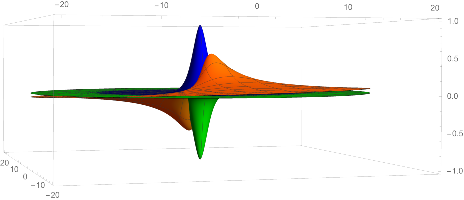
Figure 1: We show the magnetic field $B^{1}$ associated to a vortex with winding number $m^{(1)}=1$, (blue), $m^{(2)}=-1$ (green) and the magnetic field associated to the field $a_{i}$ (orange). Parameters have been chosen so that $g^{a}=1$ and $\eta^{a}=1$ for $a=1,2$.

We have found numerical solutions of Eqs. (29)-(31) by using a relaxation method. We have analyzed different topological sectors with different winding numbers $(m^{(1)},m^{(2)})$ and fluxes $B^{a}$

$$\Phi^{a}=\int d^{2}xB^{a}=\int d^{2}xF_{12}^{a}=\frac{2\pi}{g^{a}}m^{a}$$ (33)

We show in Fig.1 a solution for the case in which the topological numbers $m^{(1)}=1$ and $m^{(2)}=-1$, and where for simplicity we have set $g^{(1)}=g^{(2)}=1$ and $\eta^{(1)}=\eta^{(2)}$. The upper peak (in blue) corresponds to the magnetic field associated with the vortex with winding number $m^{(1)}=1$, and the lowest one to the magnetic field of the vortex with $m^{(2)}=-1$. In the same plot (in orange) we show the $\tilde{B}$ field defined in Eq. (32), which present a double peak structure. We remark that the particular (mirror) symmetry of the figures originates from our choices for $\eta^{a}$ and $m^{a}$ but more generic cases can be considered without additional computational effort.

Notice that the sources of this generalized magnetic field are the vector potentials of the $U(1)\times U(1)$ sector via the term $\sum_{a}\epsilon_{ia}A_{i}^{a}$. Thus, both $U(1)$ gauge fields contribute to the $\tilde{B}$ field. Nevertheless, it is enough to have only one of these gauge fields different from zero to produce a non-zero $\tilde{B}$ field. Indeed in Fig 2 we display contour plots of the $\tilde{B}$ field for two different choices of gauge fields of the $U(1)\times U(1)$ sector. Panel $(a)$ corresponds to the contour plot of $\tilde{B}$ associated to the Fig 3, this is $(m^{(1)},m^{(2)})=(1,-1)$. Panel $(b)$, corresponds to a contour plot of $\tilde{B}$ for the case $(m^{(1)},m^{(2)})=(1,0)$, where only the $A^{(1)}$ acts as a source for $\tilde{B}$. Notice that not only the intensity of the field changes depending on the choice of $m^{a}$ but also figure in the panel (b) is rotated with respect to the one in panel $(a)$.

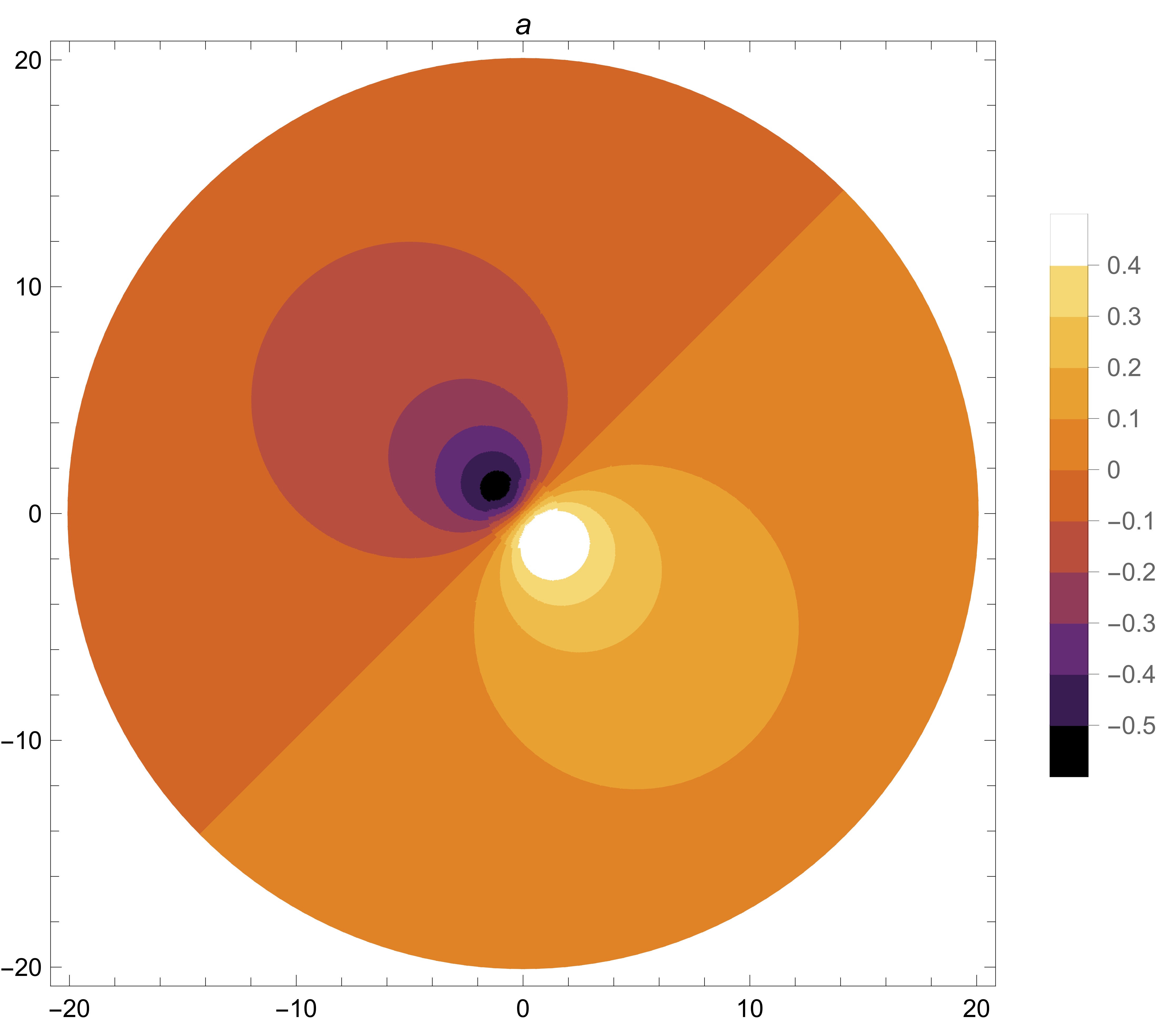
(a) sector (1,-1)

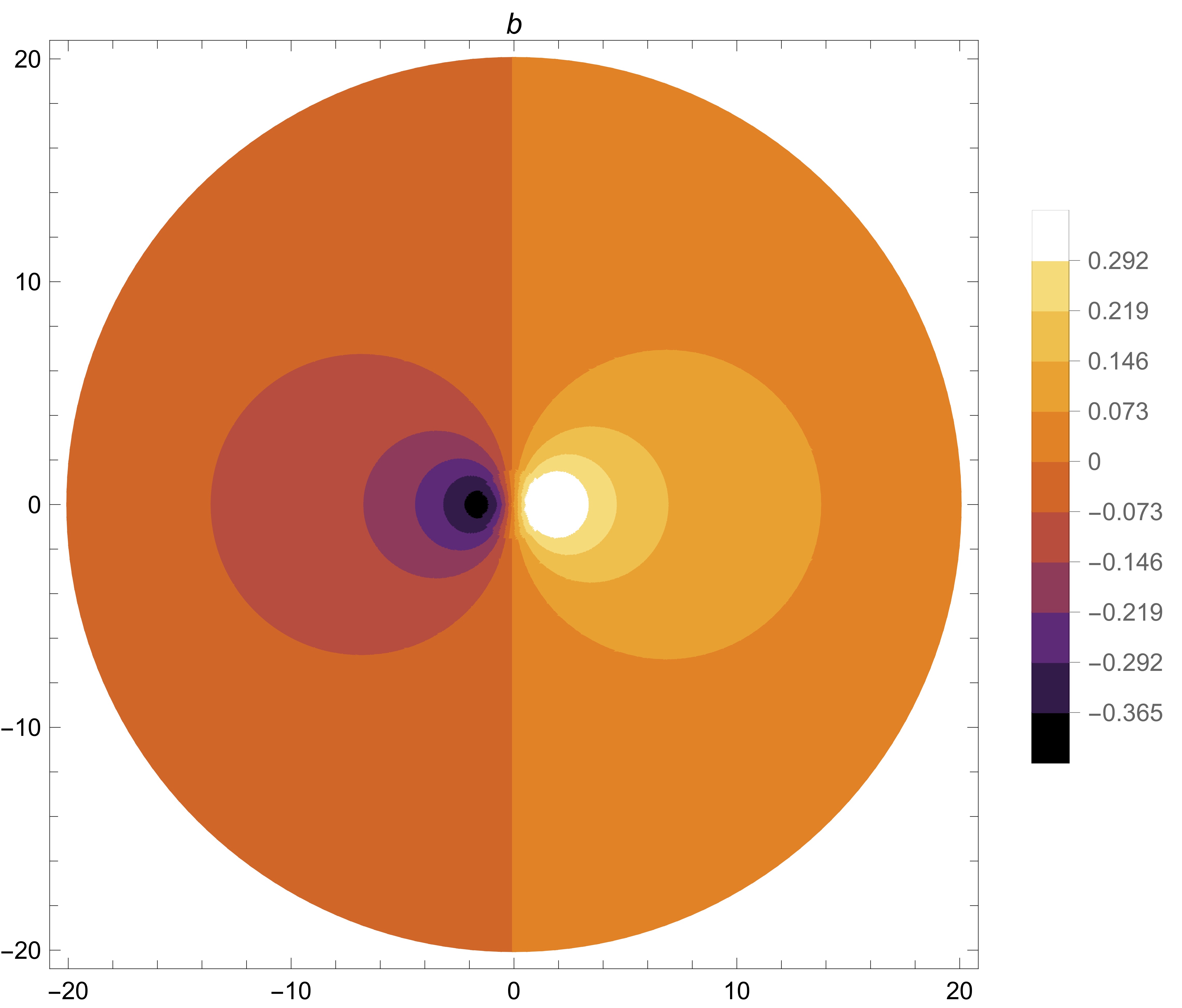
(b) sector (1,0)

Figure 2: Contour plots for the magnetic field associated to the field $\tilde{B}[a_{i}]$ for different winding numbers $(m^{(1)},m^{(2)})$. Parameters have been chosen so that $g^{a}=1$ and $\eta^{a}=1$ . Panel $(a)$ corresponds to contour plots for sector $(1,-1)$ while panel $(b)$ to sector $(1,0)$ .

Looking in more detail to panel $(b)$ in Fig 2, the contour plot looks qualitatively very similar to those of the magnetic field produced by a magnetic dipole placed outside the $(x,y)$ plane, at a certain height in a $z$ axis in three spatial dimensions, as represented schematically in Fig 3 for the $A^{(1)}$ field. In this figure we display the $B^{(1)}$ magnetic field tube (in light blue), and the two effective magnetic dipoles $\vec{\mu}$ (represented as orange arrows) associated to the $\tilde{B}$ field.

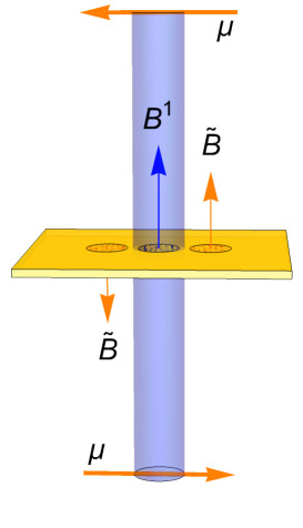
Figure 3: We represent in three spatial dimensions the magnetic field associated to a $B^{(1)}$ vortex with $m^{(1)}=1$, (light blue) and the $\tilde{B}$ field associated to $a_{i}$ (orange). Orange arrows $\mu$ represent the two effective magnetic dipoles, in this case in the $x$ direction.

Notice that the direction of the dipole is correlated with the flavor of the gauge field ($a=1$ in this case). Had we chosen, the other flavor $a=2$, the orientation of the dipole would be different. In fact, panel $(b)$ of Fig 2. results from the superposition of these cases.

Figure 4: Plot of the density $j_{0}^{m}$ for the $(1,-1)$ sector . Parameters have been chosen so that $g^{a}=1$ and $\eta^{a}=1$

Associated to the generalized gauge transformation of the $V_{i}$ field, a conserved (and gauge invariant) density $j_{0}^{m}$ was identified in Ref [1],,

$$j_{0}^{m}=\epsilon_{ij}\partial_{i}V_{j}+{\cal A}-r_{i}\epsilon_{ij}J^{m}_{0j}$$ (34)

with

$$J^{m}_{0j}=\sum_{l}\epsilon_{jl}B^{(l)}$$ (35)

In our case $j_{0}^{m}$ reduces to

$$j_{0}^{m}=xB^{(1)}+yB^{(2)}$$ (36)

We show in Fig. 4 a plot of this density $j_{0}^{m}$ for the case in in which $(m^{(1)},m^{(2)})=(1,-1)$. Similar plots can be obtained for the different sectors.

The Lagrangian (1) proposed in [1], when coupled to appropriate currents leads to Gauss law of a symmetric tensor gauge theory coupled to an external electric charge which encodes conservation not only of such charge but also conservation of an electric dipole moment [7]. In the present work, we have shown that the model described by Lagrangian (6), presents an interesting magnetics sector where in addition to the Nielsen-Olesen type vortex solutions typical of the standard $U(1)$ Higgs models, the coupling between the gauge fields and the vector field $V_{i}$ gives rise to additional magnetic fields which are qualitatively similar to those produced by an effective magnetic dipole as reflected by the conserved density $j_{0}^{m}$.

A relevant question that arises is what could it be the role of this kind of structures in fracton models. Even a more interesting situation could be expected if in addition to Maxwell term considered here, a Chern-Simons term is added . It is well-known that in the presence of Chern Simons term in the standard case vortices that carry both, electric and magnetic charge are present [12]-[13]. It is also well known that BPS equations can be found for conveniently tuned models both in the relativistic and non-relativistic cases [14]-[16]. We expected that the analysis presented here can be also applied to this case. We hope to report on this issue soon.

Acknowledgments: F.A.S. is financially supported by PIP-CONICET (PIP688), and UNLP grants X910. G.S.L. is financially supported by PICT2016-1212, PIP 11220150100653CO, Conicet, y UBACYT 20020170100496BA.

References

- [1] L. Radzihovsky and M. Hermele, Phys. Rev. Lett. 124, 050402 (2020)
- [2] M. Shifman, Advanced topics in Quantum Feld Theory, Cambridge University Press, Cambridg, UK, 2012.
- [3] E. Fradkin, Field Theories of Condensed Matter Physics, Cambridge University Press,Cambridge, UK (2013).
- [4] C. Chamon, Phys. Rev. Lett. 94, 040402 (2005).
- [5] , M. Pretko, Phys. Rev. B 95, 115139 (2017); M. Pretko, Phys. Rev. B 96, 125151 (2017) .
- [6] R. M. Nandkishore and M. Hermele, Ann. Rev. Condensed Matter Phys. 10, 295 (2019).
- [7] M. Pretko, X. Chen and Y. You, Int. J. Mod. Phys. A 35, 2030003 (2020).
- [8] Sagar Vijay, Jeongwan Haah, and Liang Fu, Phys. Rev. B 92, (2015) 235136.
- [9] E. B. Bogomolny, Sov. J. Nucl. Phys. 24 (1976) 449 [Yad. Fiz. 24, 861 ((1976).
- [10] H. J. de Vega and F. A. Schaposnik, Phys. Rev. D 14, 110 (1976).
- [11] J. D. Edelstein, C. Nunez and F. Schaposnik, Phys. Lett. B 329 (1994) 39 (2008).
- [12] S. K. Paul and A. Khare, Phys. Lett. B 174, 420 (1986) Erratum: [Phys. Lett. B 177, 453 (1986)].
- [13] H. J. de Vega and F. A. Schaposnik, Phys. Rev. Lett. 56, 2564 (1986).
- [14] J. Hong, Y. Kim and P. Y. Pac, Phys. Rev. Lett. 64 (1990) 2230.
- [15] R. Jackiw and E. J. Weinberg, Phys. Rev. Lett. 64 (1990) 2234.
- [16] R. Jackiw and S. Y. Pi, Phys. Rev. D 42, 3500 (1990) Erratum: [Phys. Rev. D 48, 3929 (1993)].