Application of the third RIT binary black hole simulations catalog to parameter estimation of gravitational waves signals from the LIGO-Virgo O1/O2 observational runs

Abstract

Using exclusively the 777 full numerical waveforms of the third Binary Black Holes RIT catalog, we reanalyze the ten black hole merger signals reported in LIGO/Virgo’s O1/O2 observation runs. We obtain binary parameters, extrinsic parameters, and the remnant properties of these gravitational waves events which are consistent with, but not identical to previously presented results. We have also analyzed three additional events (GW170121, GW170304, GW170727) reported in Venumadhav et al. (2020) and found closely matching parameters. We finally assess the accuracy of our waveforms with convergence studies applied to O1/O2 events and found them adequate for current estimation of parameters.

I Introduction

The Advanced LIGO LIGO Scientific Collaboration et al. (2015) and Virgo Acernese et al. (2015) ground-based gravitational wave (GW) detectors have identified several coalescing compact binaries The LIGO Scientific Collaboration and the Virgo Collaboration (2016); Abbott et al. (2016) (The LIGO Scientific Collaboration and the Virgo Collaboration); Abbott et al. (2017); The LIGO Scientific Collaboration et al. (2017a, b, c) and characterized their properties with Bayesian inference The LIGO Scientific Collaboration and the Virgo Collaboration (2016); Abbott et al. (2016) (The LIGO Scientific Collaboration and the Virgo Collaboration); Abbott et al. (2017); The LIGO Scientific Collaboration et al. (2017a, b, c, 2019); Pankow et al. (2015a); Lange et al. (2018); Veitch et al. (2015). As observatories’ sensitivities increase, many more observations are expected Abbott et al. (2016), and some will be even better resolved. With more and some very informative events, these GW observations pose a challenge to source parameter inference: barring substantial improvements, systematic uncertainty in our models will increasingly limit our ability to draw the sharpest possible conclusions from each observation.

Our understanding of the gravitational waves from merging binary black holes follows from numerical solutions to Einstein’s equations. Numerical relativity breakthroughs Pretorius (2005); Campanelli et al. (2006); Baker et al. (2006) led to detailed predictions of the gravitational waves from the late inspiral, plunge, merger, and ringdown of black-hole-binary systems (BHB). These predictions helped to accurately identify the first direct detection Abbott et al. (2016a) of gravitational waves with such binary black hole systems Abbott et al. (2016b, c, d, 2017a) and match them to targeted supercomputer simulations Abbott et al. (2016e, f); Lovelace et al. (2016). There have been several significant efforts to coordinate numerical relativity simulations to support gravitational wave observations. These include the numerical injection analysis (NINJA) project Aylott et al. (2009a, b); Ajith et al. (2012); Aasi et al. (2014), the numerical relativity and analytical relativity (NRAR) collaboration Hinder et al. (2014), and the waveform catalogs released by the SXS collaboration Mroue et al. (2013); Blackman et al. (2015); Chu et al. (2016); Boyle et al. (2019), Georgia Tech, Jani et al. (2016), and RIT Healy et al. (2017a, 2019); Healy and Lousto (2020). Numerical relativity simulations have been directly compared to GW observations to draw inferences about binary parameters, starting with GW150914 Abbott et al. (2016e); Lovelace et al. (2016); Healy et al. (2019) and continuing through GW170104 Abbott et al. (2017b); Healy et al. (2018a), GW170608 Abbott et al. (2017c), the analysis in GWTC-1 The LIGO Scientific Collaboration et al. (2019), and GW190521 The LIGO Scientific Collaboration et al. (2020a, b). Further discussion of these methods can be found in Lange et al. (2017, 2017); Lange (2016). Previous comparisons of GW observations to banks of NR simulations have used heterogeneous sets of NR simulations, with differences in accuracy standards and choices for initial starting separation. Only the analysis of GW190521 presented posteriors for all intrinsic parameters of a generic quasicircular binary black hole, allowing for precessing spins.

In this work, we analyze all proposed candidate BBH observations reported before the latest observing run (O3) with a single, consistent set of numerical relativity simulations: the simulations in the third release of the RIT public catalog Healy and Lousto (2020). These simulations adopt consistent resolutions and initial conditions. We demonstrate that direct comparisons to numerical relativity simulations can recover all astrophysically interesting properties of merging binary black holes, including the effect of misaligned spin.

This paper is organized as follows. In Sec. II we review the methods we use to infer the intrinsic and extrinsic parameters of compact binary sources, via direct comparison to our specific set of numerical relativity simulations. Specifically, following Lange et al. (2017), on the grid of simulations we evaluate the Bayesian likelihood maximized over extrinsic parameters, using RIFT Lange et al. (2018). We generate posterior distributions by interpolating the resulting (marginal) likelihood distribution. In Sec. III we use the waveform catalog to estimate the binary black hole parameters that best match the ten BBH signals reported in the first and second LIGO-Virgo observing runs Abbott et al. (2019). We find our method can produce posteriors quite consistent with previously reported results. Our headline posterior inferences differ principally because we adopt different prior distributions for the binary mass, mass ratio, and spin Vitale et al. (2017). We conclude in Sec. IV with a discussion of the future use of this catalog for parameter inference of new gravitational waves events and the extensions of this work to more generic precessing binaries.

II Application of the waveforms catalog to parameter estimation of Binary Black holes

II.1 Simulations

The third release of the RIT public catalog Healy and Lousto (2020) of numerical relativity black-hole-binary waveforms http://ccrg.rit.edu/~RITCatalog consists of 777 accurate simulations that include 300 precessing and 477 nonprecessing binary systems with mass ratios $q=m_{1}/m_{2}$ in the range $1/15\leq q\leq 1$ and individual spins up to $S_{i}/m_{i}^{2}=0.95$. The catalog also provides initial parameters of the binary, trajectory information, peak radiation, and final remnant black hole properties. The catalog includes all waveform modes $\ell\leq 4$ of $\psi_{4}$ and the strain $h$ (both extrapolated to null-infinity) and is updated to correct for the center of mass displacement during inspiral and after merger Healy and Lousto (2020).

The third RIT public catalog has two families of simulations salient to our comparison. First, the RIT catalog has many nonprecessing simulations, displayed in Fig. 5 of Ref. Healy and Lousto (2020). The RIT catalog also has many precessing simulations, performed with similar settings and to a consistent standard. To simplify the large precessing parameter space, we focus on systems where one black hole is nonspinning, and vary the spin orientation of the other. Currently this set of simulations consists of nine different mass ratio families as displayed in Fig. 8 of Ref. Healy and Lousto (2020) with up to 40 different spin orientations per family. We supplement the new simulations in this catalog release with those reported in Ref.  Lousto and Zlochower (2013); Zlochower and Lousto (2015)

II.2 Direct comparison of NR to GW observations

We can directly compare any of our simulations to real or synthetic gravitational wave observations by scaling that simulation and its predictions to a specific total redshifted mass $M_{z}$ and then marginalizing the likelihood for the gravitational wave data over all extrinsic parameters Pankow et al. (2015b); Abbott et al. (2016e); Lange et al. (2017); O’Shaughnessy et al. (2017); Lange et al. (2018): the seven coordinates characterizing the spacetime coordinates and orientation of the binary relative to the earth. Specifically the likelihood of the data given Gaussian noise has the form (up to normalization)

$$\ln{\cal L}(\bm{\lambda};\theta)=-\frac{1}{2}\sum\limits_{k}\langle h_{k}(\bm{\lambda},\theta)-d_{k}|h_{k}(\bm{\lambda},\theta)-d_{k}\rangle_{k}-\langle d_{k}|d_{k}\rangle_{k},$$ (1)

where $h_{k}$ are the predicted response of the k^th detector due to a source with parameters ($\bm{\lambda}$, $\theta$) and $d_{k}$ are the detector data in each instrument k; $\bm{\lambda}$ denotes the combination of redshifted mass $M_{z}$ and the remaining intrinsic parameters (mass ratio and spins; with eccentricity $\approx 0$) needed to uniquely specify the binary’s dynamics; $\theta$ represents the seven extrinsic parameters (4 spacetime coordinates for the coalescence event and 3 Euler angles for the binary’s orientation relative to the Earth); and $\langle a|b\rangle_{k}\equiv\int_{-\infty}^{\infty}2df\tilde{a}(f)^{*}\tilde{b}(f)/S_{h,k}(|f|)$ is an inner product implied by the k^th detector’s noise power spectrum $S_{h,k}(f)$. In practice we adopt a low-frequency cutoff f_min so all inner products are modified to

$$\langle a|b\rangle_{k}\equiv 2\int_{|f|>f_{\rm min}}df\frac{[\tilde{a}(f)]^{*}\tilde{b}(f)}{S_{h,k}(|f|)}.$$ (2)

For our analysis of GW150914, we adopt the same noise power spectrum employed in previous work Abbott et al. (2016e); Lange et al. (2018). For each simulation and each detector-frame mass $M_{z}=(1+z)M$, we then compute the marginalized likelihood

$${\cal L}_{\rm marg}(\lambda)=\int d\theta p(\theta){\cal L}(\bm{\lambda},\theta)$$ (3)

where $\lambda$ denotes the simulation parameters and the redshifted mass $M_{z}$ and where $p(\theta)$ is a conventional prior on the extrinsic parameters.

For each simulation, the marginalized likelihood in Eq. (3) is a one-dimensional function of $M_{z}$. In practice, we explore a small range of redshifted masses for each simulation, to be sure we cover the region near the peak values well; see Abbott et al. (2016e); Lange et al. (2017).

II.3 Intrinsic coordinate systems and priors for binaries

We characterize the intrinsic parameters of BH binaries with the (redshifted) components masses $m_{1,z},m_{2,z}$ and dimensionless spins $\bm{\chi}_{i}$. However, we will also use several other coordinates to characterize binary properties when performing parameter inference. We use the familiar total mass $M_{z}=m_{1,z}+m_{2,z}$ and mass ratio $q=m_{1,z}/m_{2,z}$, where we require $m_{2,z}>m_{1,z}$. For binary spins, we principally characterize the effects of aligned spin in the strong field with $S_{hu}$, defined by

$$M^{2}\,S_{hu}=\left((1+\frac{1}{2q})\,\vec{S}_{1}+(1+\frac{1}{2}q)\,\vec{S}_{2}\right)\cdot\hat{L},$$ (4)

to describe the leading effect of hangup on the full numerical waveforms Healy and Lousto (2018). Motivated by work on post-Newtonian inspiral, we also use the variable Ajith et al. (2011)

$$M^{2}\,\chi_{eff}=\left((1+\frac{1}{q})\,\vec{S}_{1}+(1+q)\,\vec{S}_{2}\right)\cdot\hat{L}$$

to characterize the effects of aligned spins.

We adopt four distinct joint prior distributions over these intrinsic parameters. For the first family, appropriate to generic quasicircular binaries, we adopt the generic quasicircular priors used in previous work The LIGO Scientific Collaboration et al. (2019); Lange et al. (2018): jointly uniform in $m_{1,z},m_{2,z}$; a uniformly isotropic spin orientation distribution for both spins; and magnitudes $|\bm{\chi}_{1}|$, $|\bm{\chi}_{2}|$ both uniform from 0 to 1. For the second family, appropriate to nonprecessing binaries, we adopt a familiar nonprecessing prior The LIGO Scientific Collaboration et al. (2019); Lange et al. (2018): jointly uniform in $m_{1,z},m_{2,z}$; both spin angular momenta aligned with $\hat{L}$ (also denoted the $z$ axis); and $\chi_{i,z}$ drawn from the “z prior” between $[-1,1]$ Lange et al. (2018). [The “z prior” is equal to the marginal distribution of $\chi_{i,z}$ if $\bm{\chi}_{i}$ are isotropic and have magnitudes uniform from 0 to 1. To the extent transverse spins have no impact on the likelihood, an aligned result with the z prior will agree with generic quasicircular inference using the isotropic/uniform-magnitude prior.] For the third family, also appropriate to nonprecessing binaries, we adopt a different prior: $M_{z},q,\chi_{1,z},\chi_{2,z}$ all jointly uniform over their allowed range, with $q\leq 1$ and $|\bm{\chi}_{i}|<1$. For the fourth family, appropriate to a single precessing spin, we allow the polar spin angles to be uniform in $\theta,\phi$; $|\bm{\chi}_{i}|$ to be uniform from [0,1]; the parameter $q\in[0.2,2]$, where $q<1$ means the more massive BH is spinning and $q>1$ means the less massive BH is spinning; and $M_{z}$ is uniform. Unless otherwise noted, all posterior distributions and credible intervals are generated using the last two sets of prior assumptions.

The precessing simulations used here explore only one of the two precessing degrees of freedom. For the short binary black hole GW signals studied here, however, observations only weakly constrain the subdominant effect of the smaller objects’ spin. Targeted studies of precessing, two spin configurations have been performed for GW170104 Healy et al. (2018a) and GW190521 The LIGO Scientific Collaboration et al. (2020a).

II.4 Likelihood interpolation and posterior generation

Following previous work Lange et al. (2018, 2017), we interpolate the marginal likelihood between simulation parameters. Because of the two distinct groupings and limited parameter space coverage, we perform two independent interpolations over the two distinct sets of simulations: nonprecessing and precessing. In both cases, we use Gaussian process (GPR) regression to interpolate between and extrapolate outside the parameter space covered by our simulations. Posterior distributions are generated by sampling from our prior distributions, weighting by the likelihood. When employing the first two conventional priors, we use the “construct intrinsic posteriors” (CIP) program, an interpolation and posterior-generating code provided by RIFT (Rapid Inference via iterative fitting), which uses a squared-exponential plus white noise kernel Lange et al. (2018). When employing the uniform in $M,q,|\bm{\chi}|$ prior, we use an independent implementation, also using a GPR with a squared exponential and white noise kernel.

Specifically, for one family of results, we only use nonprecessing simulations to compare to GW observations. For the other family of results, we use only precessing simulations. For the final black hole parameters, we use the nonprecessing simulations.

For nonprecessing simulations, we can also perform a 3-dimensional GPR fit of $\ln{\cal L}(q,\chi_{1},\chi_{2})$ by maximizing over the total mass for each simulation. We perform both analyses and compare results to check consistency and robustness of the algorithm. Finally, for the purposes of illustration, we can also perform a 2-dimensional GPR fit of $\ln{\cal L}(q,S_{hu})$ or ${\cal L}(q,\chi_{eff})$ by maximizing over total mass and assuming the remaining spin degrees of freedom do not impact the marginal likelihood.

II.5 Estimation of extrinsic parameters

To roughly estimate the extrinsic parameters of the events, we look at up to 100 of the top (precessing and non-precessing) simulations per event and output the samples from the RIFT analysis before marginalization. We then apply the technique described in Lange et al. (2018) to infer the extrinsic parameters, assuming the intrinsic parameters of NR simulations cover a representative region of the posterior. Unlike the interpolation-based methods used for intrinsic parameters, we do not presently correct for the finite, discrete simulation coverage over the intrinsic parameter space when inferring extrinsic binary parameters.

II.6 Simulated versus signal waveform comparison

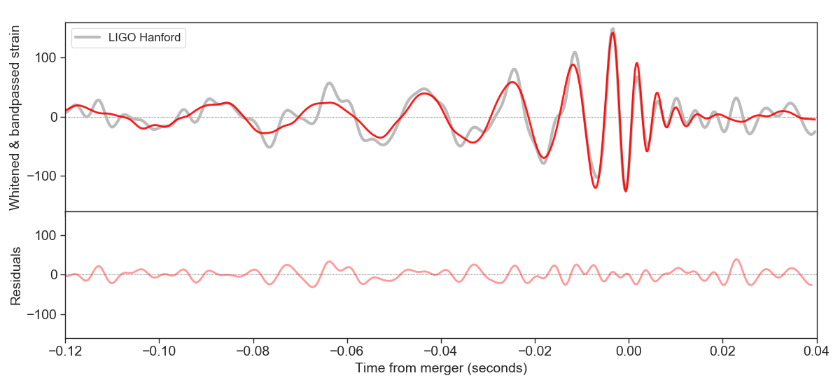
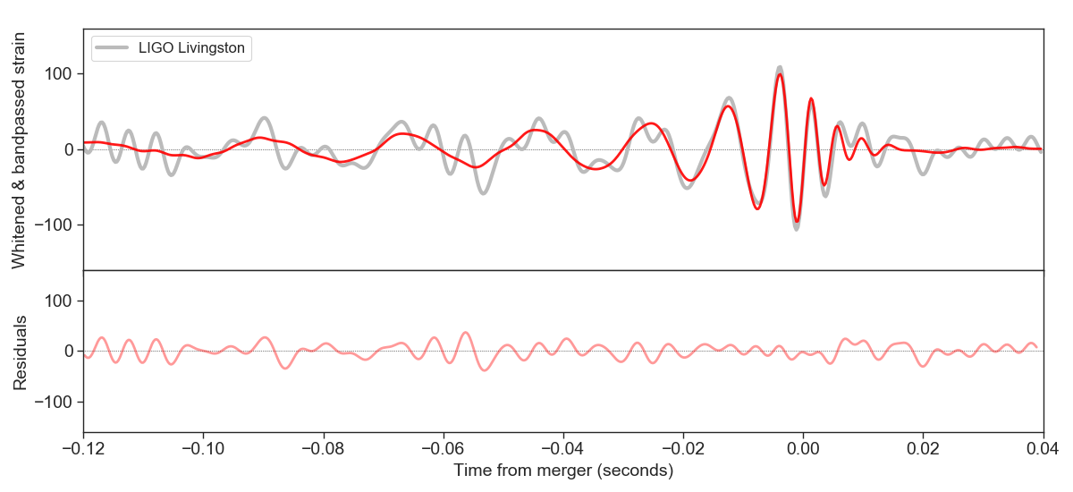
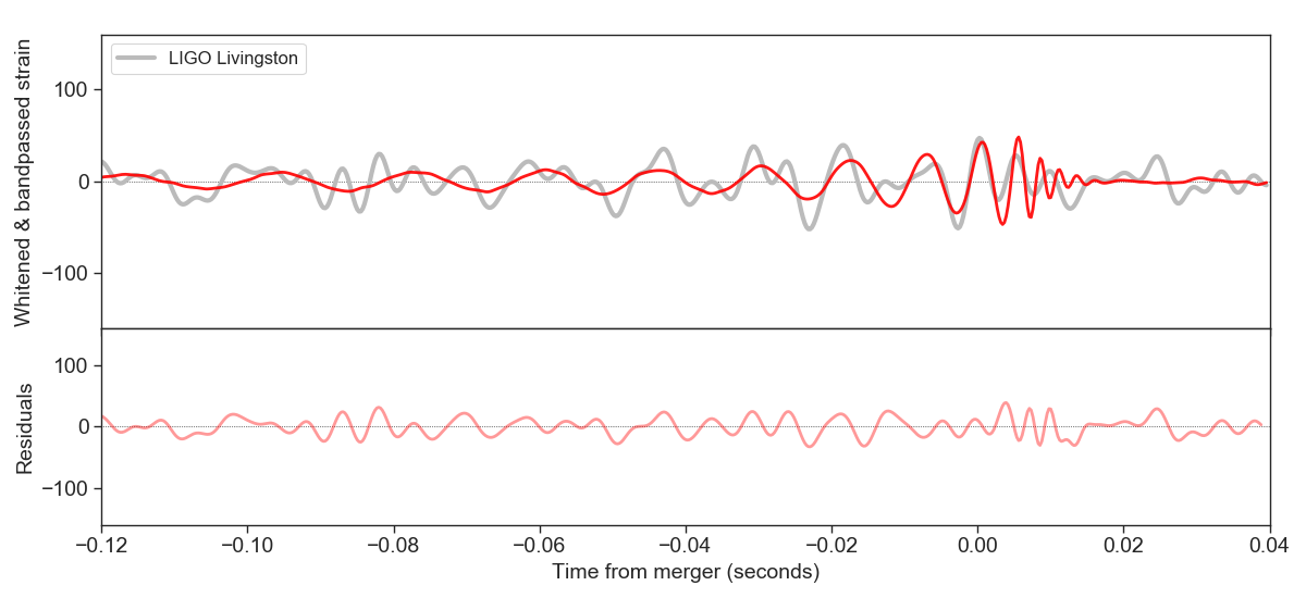
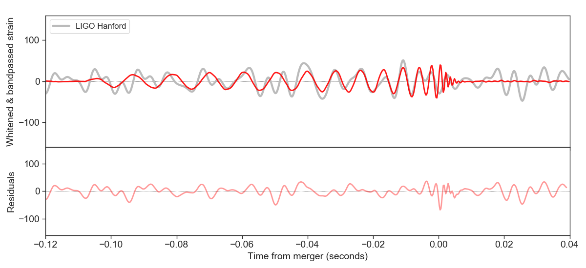
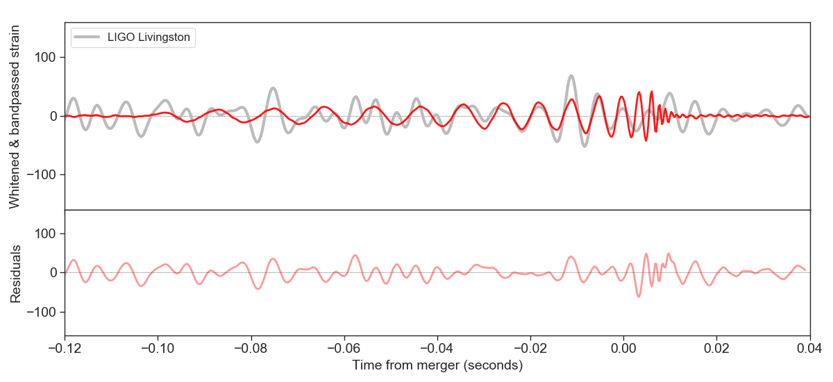
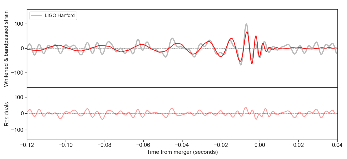
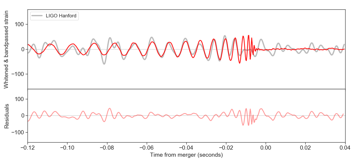
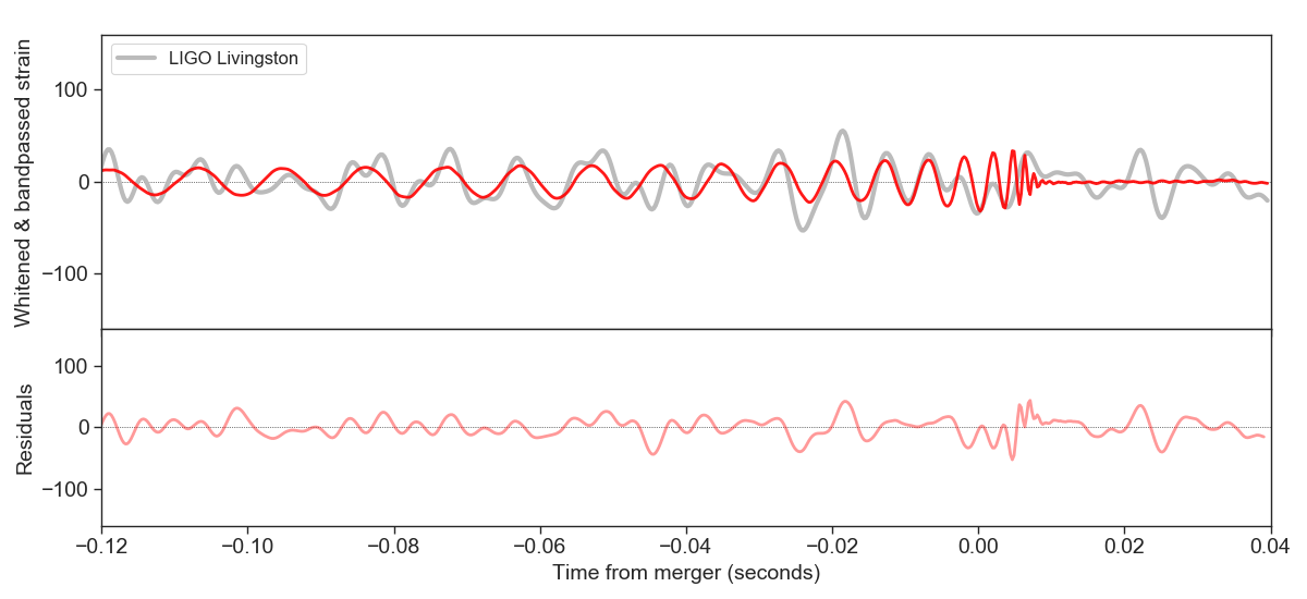
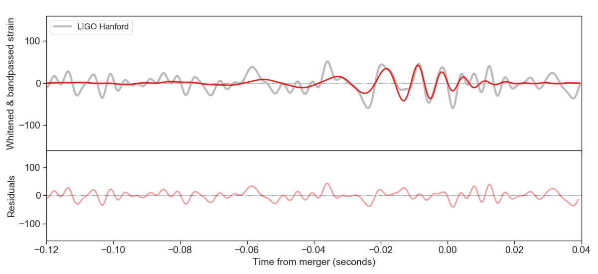
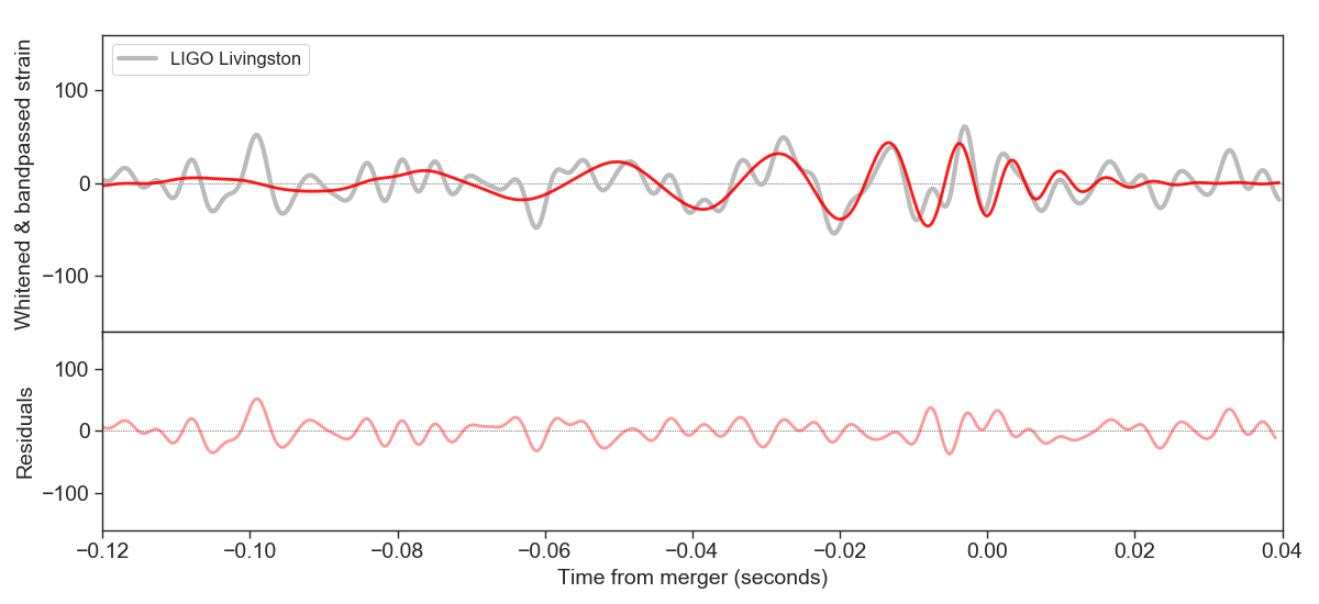
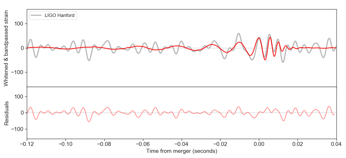
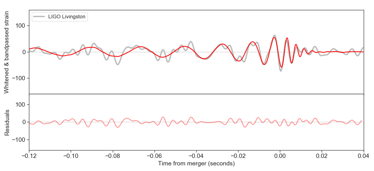
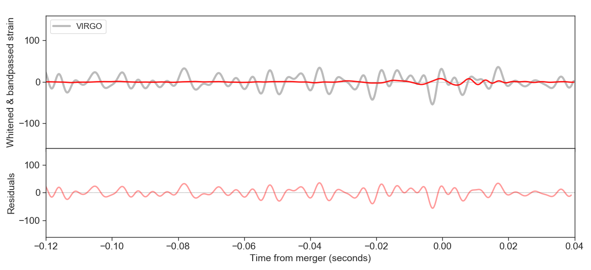
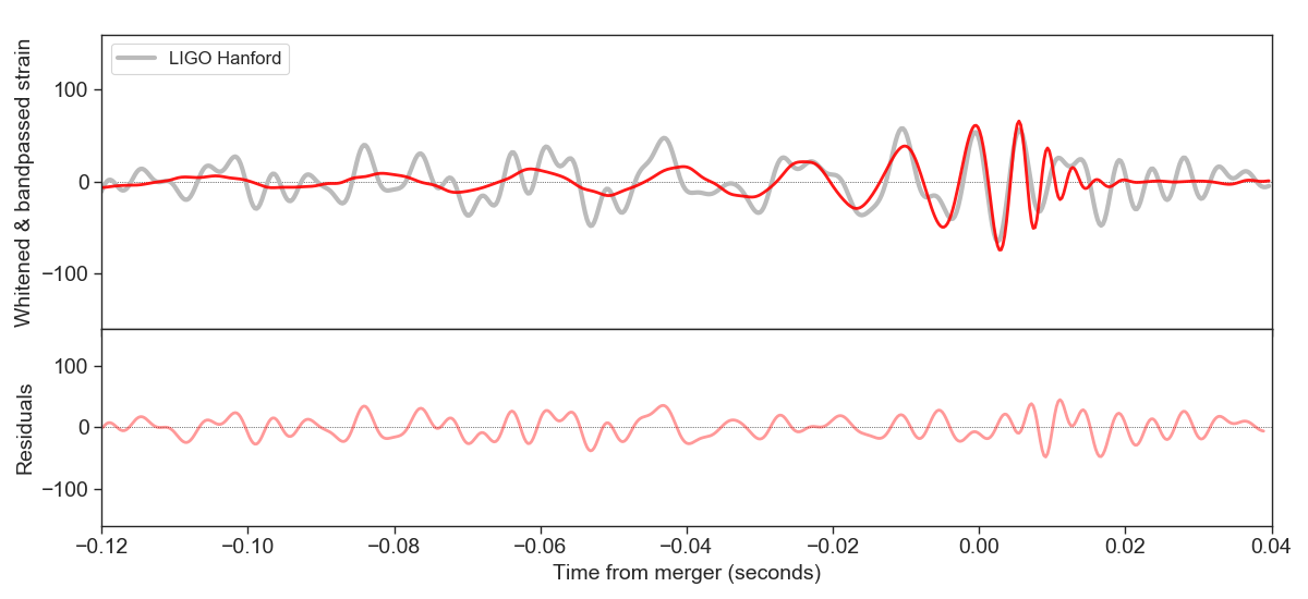
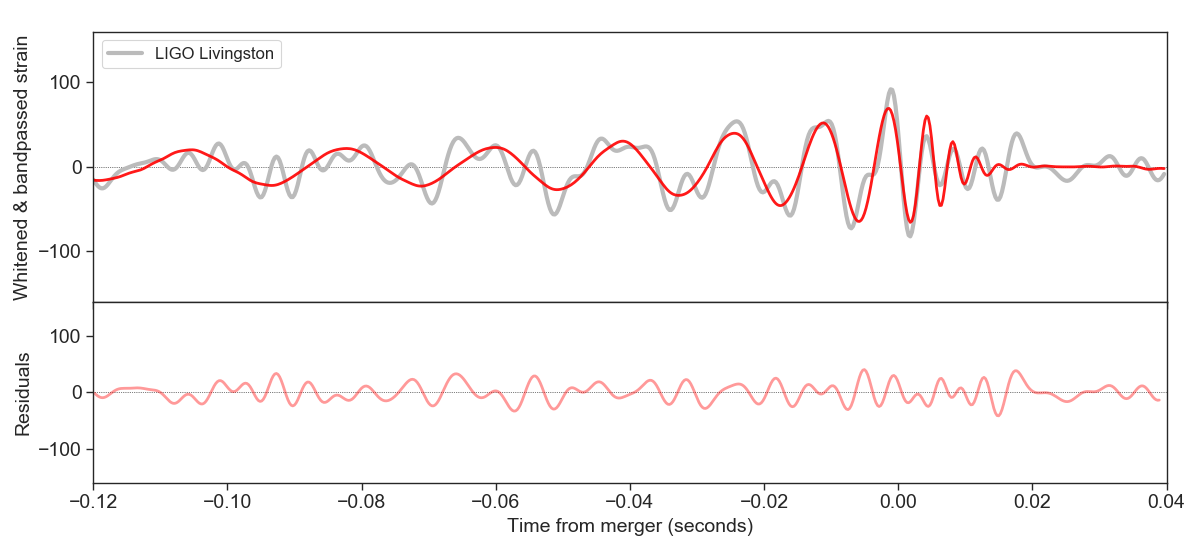
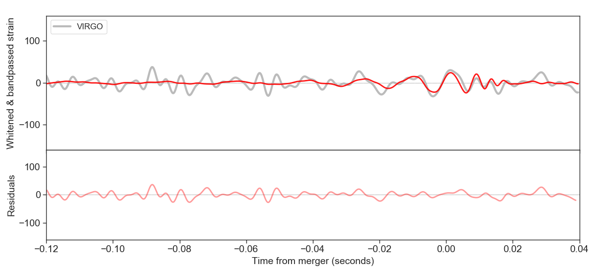
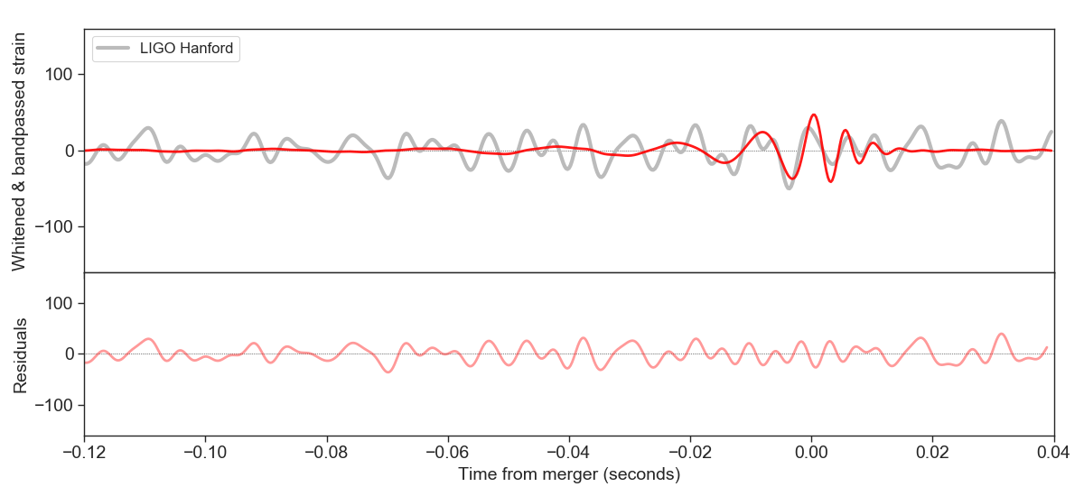
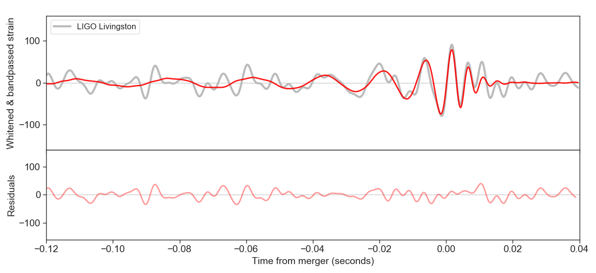
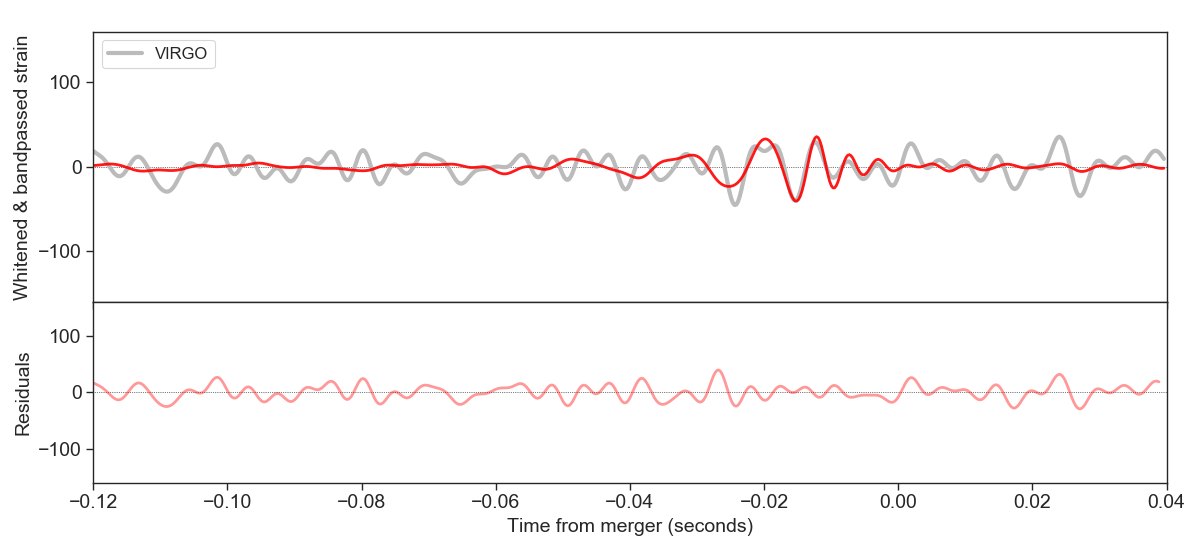
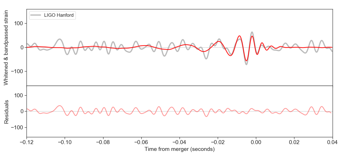
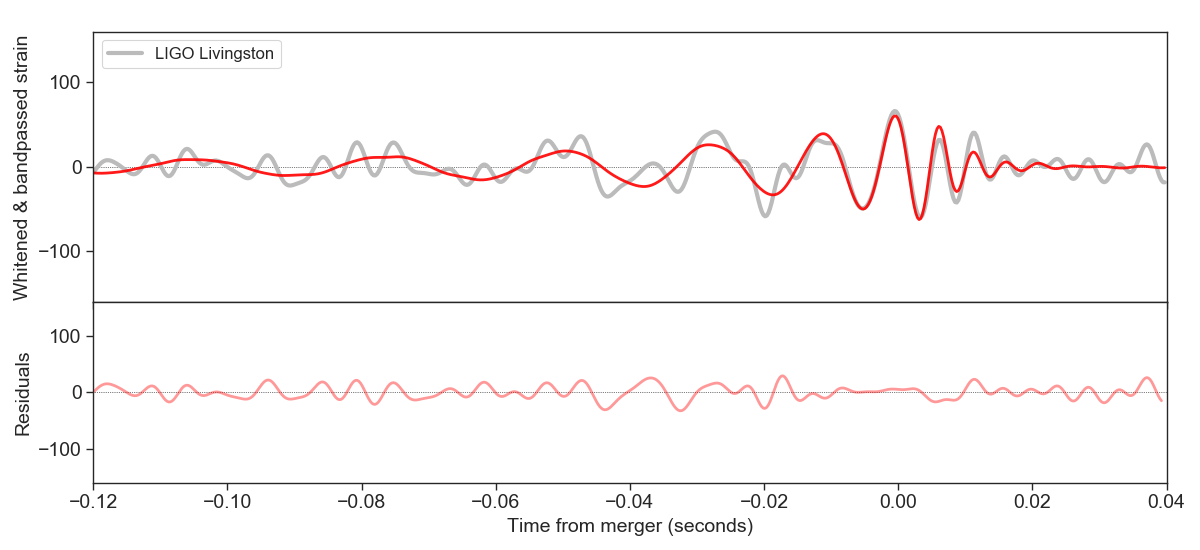
We use standard techniques Abbott et al. (2016e); Lange et al. (2017) to directly compare GW150914 (See Fig. 10 of Healy et al. (2019)) and other O1/O2 BBH signals to our simulations. For each simulation, direct comparison of our waveforms to the data selects a fiducial total mass which best fits the observations, as measured by the marginalized likelihood. We can for each simulation select the binary extrinsic parameters, like event time and sky location which maximize the likelihood of the data, given our simulation and mass. Then, using these extrinsic parameters, we evaluate the expected detector response in the LIGO Hanford (H1) and Livingston (L1) instruments. For each of the ten O1/O2 signals we will display these reconstructions for the highest log-likelihood NR waveform of the nonprecessing and precessing simulations in our catalog. They directly compare to the signals as observed by LIGO H1 and L1 (and Virgo, when available) and with each other. The lower panels show the residuals of the signals with respect to the RIT simulations. A similar analysis was performed in Ref. Healy et al. (2018b), Figures 4-6, for the GW170104 event.

III Parameter estimation of the BBH signals in O1/O2 LIGO runs

In this section, we analyze the ten events reported by LIGO and three additional binary black hole candidates, using direct comparison to numerical relativity. We provide two sets of our own estimates of binary intrinsic parameters, derived first assuming strict spin-orbit alignment (Table 1) and then allowing for a single precessing spin (Table 2), both calculated using our preferred priors (i.e., uniform in $M_{z},q$). We also provide our estimates for binary extrinsic parameters (Table 3), using a standard flat $\Lambda$CDM cosmology with Hubble parameter $H_{0}=67.9$km/s/Mpc and matter density parameter $\Omega_{m}=0.306$ Ade et al. (2016). We provide quantitative comparison between our results and previous analyses of these events using the Jensen-Shannon divergence Mateos et al. (2017) (JSD) (Table 4), both when using our preferred priors and when using priors consistent with previous work. To simplify our presentation, we have selected four exemplary events to illustrate our inferences in greater detail: GW159014, GW170104, GW170729, and GW170814.

Table 1: Parameter estimation of the mass ratio $q$, the individual spins $a_{1}$ and $a_{2}$, the total mass of the system in the detector frame, $M_{total}=m_{1}+m_{2}$ and the effective spin variables $S_{hu}$ and $\chi_{eff}$, at the 5,50,95 percentiles. The last column gives the Bayes Factor between uniform aligned spins and nonspinning systems.

Event	$f_{min}$	Max($\ln{\cal L}$)	$q=m_{1}/m_{2}$	$a_{1}$	$a_{2}$	$M_{total}/M_{\odot}$	$S_{hu}$	$\chi_{eff}$	B.F.
GW150914	30	296.6	$0.9436^{+0.0520}_{-0.2216}$	$-0.4434^{+1.1750}_{-0.4468}$	$0.3388^{+0.3602}_{-1.1620}$	$71.7^{+4.}_{-4.1}$	$-0.0342^{+0.1122}_{-0.1092}$	$-0.0418^{+0.1166}_{-0.1048}$	0.295
GW151012	50	23.7	$0.7111^{+0.2621}_{-0.4510}$	$0.0768^{+0.7832}_{-0.9114}$	$0.3218^{+0.5694}_{-0.8580}$	$47.5^{+20.4}_{-8.4}$	$0.1924^{+0.4518}_{-0.4018}$	$0.1826^{+0.4464}_{-0.3888}$	0.865
GW151226	80	27.4	$0.6782^{+0.2741}_{-0.3301}$	$0.2056^{+0.6858}_{-1.0484}$	$0.2524^{+0.6656}_{-0.8224}$	$23.3^{+4.5}_{-3.9}$	$0.2034^{+0.3908}_{-0.5448}$	$0.1962^{+0.3930}_{-0.5240}$	-
GW170104	30	75.7	$0.9167^{+0.0732}_{-0.3412}$	$-0.1328^{+1.0370}_{-0.7962}$	$-0.0490^{+0.9612}_{-0.8476}$	$61.0^{+5.4}_{-6.1}$	$-0.0212^{+0.1896}_{-0.2530}$	$-0.0216^{+0.1884}_{-0.2520}$	0.404
GW170608	80	54.2	$0.6952^{+0.2585}_{-0.3289}$	$0.3476^{+0.5460}_{-0.8888}$	$0.2302^{+0.6312}_{-0.5390}$	$22.0^{+3.1}_{-2.9}$	$0.2878^{+0.3600}_{-0.4578}$	$0.2948^{+0.3368}_{-0.4630}$	-
GW170729	20	40.5	$0.6302^{+0.3262}_{-0.2194}$	$-0.1216^{+0.9132}_{-0.7676}$	$0.6184^{+0.3286}_{-0.6140}$	$125.8^{+15.9}_{-17.1}$	$0.3568^{+0.2100}_{-0.2632}$	$0.3236^{+0.2368}_{-0.2582}$	3.145
GW170809	30	56.0	$0.8653^{+0.1247}_{-0.3600}$	$0.1476^{+0.7020}_{-1.0518}$	$0.0334^{+0.8758}_{-0.5578}$	$72.2^{+4.7}_{-6.9}$	$0.1160^{+0.1554}_{-0.2418}$	$0.1112^{+0.1566}_{-0.2286}$	0.392
GW170814	30	118.6	$0.7949^{+0.1828}_{-0.1438}$	$-0.2334^{+0.7426}_{-0.6790}$	$-0.0392^{+0.9190}_{-0.4422}$	$58.1^{+4.3}_{-3.1}$	$-0.0942^{+0.1624}_{-0.1310}$	$-0.0942^{+0.1544}_{-0.1298}$	0.254
GW170818	30	48.0	$0.8758^{+0.1107}_{-0.2936}$	$-0.2590^{+1.0278}_{-0.6498}$	$0.0984^{+0.7848}_{-0.8246}$	$76.5^{+8.3}_{-7.4}$	$-0.0304^{+0.2372}_{-0.2562}$	$-0.0348^{+0.2310}_{-0.2504}$	0.237
GW170823	30	53.0	$0.8367^{+0.1508}_{-0.3031}$	$-0.0836^{+0.9032}_{-0.7876}$	$0.1642^{+0.6982}_{-0.8892}$	$90.2^{+12.7}_{-10.9}$	$0.0528^{+0.2344}_{-0.2608}$	$0.0468^{+0.2332}_{-0.2502}$	0.295
GW170121	30	31.5	$0.8519^{+0.1327}_{-0.3086}$	$-0.2910^{+0.9282}_{-0.5978}$	$-0.2568^{+0.7024}_{-0.6102}$	$70.9^{+10.9}_{-8.3}$	$-0.2520^{+0.2942}_{-0.3036}$	$-0.2498^{+0.2872}_{-0.3010}$	0.933
GW170304	20	24.3	$0.7948^{+0.1867}_{-0.3228}$	$0.0606^{+0.7756}_{-0.8774}$	$0.3262^{+0.5890}_{-0.7760}$	$106.1^{+17.5}_{-15.1}$	$0.2066^{+0.2602}_{-0.3074}$	$0.1966^{+0.2654}_{-0.2974}$	0.822
GW170727	20	19.6	$0.8261^{+0.1569}_{-0.3062}$	$-0.1136^{+0.9198}_{-0.7688}$	$0.0200^{+0.7954}_{-0.8106}$	$103.0^{+17.5}_{-15.3}$	$-0.0108^{+0.3004}_{-0.3632}$	$-0.0136^{+0.2926}_{-0.3558}$	0.414

Table 2: Doing a GPR fit to find the highest $\ln{\cal L}$ from the 300 precessing simulations. Parameter estimation of the mass ratio $q$, the initial spin angle $\theta$ and $\varphi$, and the total mass of the system in the detector frame, $M_{total}/M_{\odot}$, at the mean of $\ln{\cal L}$ and its $90\%$ confidence ranges.

Event	$f_{min}$	Max($\ln{\cal L}$)	$q$	$\theta$	$\varphi$	$M_{total}/M_{\odot}$
GW150914	30	296.6	$0.9853^{+0.1928}_{-0.1664}$	$1.6346^{+0.2727}_{-0.2454}$	$4.1796^{+1.3440}_{-3.5406}$	$72.2^{+5.2}_{-7.7}$
GW151012	50	23.7	$0.9898^{+0.3447}_{-0.4484}$	$1.4338^{+0.9705}_{-1.2302}$	$4.0376^{+1.5588}_{-3.3854}$	$45.2^{+7.9}_{-6.8}$
GW151226	80	27.4	$0.6004^{+0.2396}_{-0.0309}$	$2.9566^{+0.1454}_{-0.1772}$	$3.6298^{+2.3424}_{-3.0473}$	$14.6^{+1.6}_{-0.7}$
GW170104	30	75.7	$0.6110^{+0.3656}_{-0.0867}$	$2.3201^{+0.6119}_{-0.7597}$	$3.6505^{+2.3776}_{-3.3137}$	$54.9^{+8.1}_{-3.6}$
GW170608	80	54.2	$0.6010^{+0.0183}_{-0.0178}$	$3.0609^{+0.0728}_{-0.1631}$	$4.4296^{+1.6349}_{-3.9571}$	$11.7^{+0.8}_{-0.6}$
GW170729	20	40.5	$0.7130^{+0.6074}_{-0.2810}$	$0.4907^{+0.7031}_{-0.4392}$	$3.3200^{+2.5843}_{-3.0065}$	$126.9^{+11.5}_{-12.2}$
GW170809	30	56.0	$0.8661^{+0.4389}_{-0.3400}$	$1.6142^{+0.9650}_{-0.9469}$	$4.0074^{+2.0326}_{-3.5186}$	$68.6^{+8.4}_{-9.1}$
GW170814	30	118.6	$1.0890^{+0.2306}_{-0.3629}$	$1.6160^{+0.5646}_{-0.4112}$	$3.7617^{+2.1948}_{-3.3847}$	$60.1^{+3.6}_{-4.2}$
GW170818	30	48.0	$0.8929^{+0.2240}_{-0.3186}$	$1.7876^{+0.7850}_{-0.4870}$	$3.6656^{+2.1489}_{-3.0857}$	$76.4^{+6.1}_{-7.7}$
GW170823	30	53.0	$1.0036^{+0.3539}_{-0.4174}$	$1.4502^{+0.8174}_{-0.9947}$	$3.2547^{+2.7583}_{-2.9123}$	$88.9^{+14.2}_{-20.3}$
GW170121	30	31.5	$1.1050^{+0.2736}_{-0.5313}$	$2.7502^{+0.3380}_{-0.9014}$	$3.1290^{+2.8670}_{-2.8381}$	$70.4^{+5.0}_{-4.7}$
GW170304	20	24.3	$0.9935^{+0.3574}_{-0.5184}$	$0.8781^{+0.9566}_{-0.7713}$	$3.1937^{+2.7716}_{-2.8827}$	$107.6^{+6.1}_{-8.9}$
GW170727	20	19.6	$1.0757^{+0.2890}_{-0.4808}$	$1.7577^{+1.1376}_{-1.1253}$	$3.1165^{+2.8582}_{-2.7948}$	$95.8^{+21.5}_{-13.5}$

Table 3: Using samples from the top $\ln{\cal L}$ simulations to estimate the extrinsic parameters. Shown are the the luminosity distance $D$, sky location r.a. and declination, and the euler angles, $\phi_{orb}$, $\iota$, and $\psi$ at the 5,50,95 percentiles. Note that the priors in this analysis is a discrete set of simulations, so the ranges are not comprehensive.

Event	$D$	r.a.	declination	$\phi_{orb}$	$\iota$	$\psi$
GW150914	$541.7794^{+130.1726}_{-229.9624}$	$2.4741^{+0.1738}_{-1.5149}$	$-1.1023^{+0.1662}_{-0.1442}$	$3.1280^{+2.8179}_{-2.8181}$	$2.6698^{+0.3474}_{-1.3776}$	$3.1578^{+2.7897}_{-2.8731}$
GW151012	$1131.1394^{+571.6106}_{-504.8474}$	$-0.6554^{+2.5200}_{-1.6497}$	$-0.0541^{+1.1431}_{-0.9482}$	$3.0769^{+2.8817}_{-2.7397}$	$1.6932^{+1.2072}_{-1.4446}$	$3.1209^{+2.8288}_{-2.7922}$
GW151226	$408.8335^{+254.4875}_{-192.2955}$	$-0.7096^{+2.6668}_{-2.1212}$	$-0.0609^{+0.9958}_{-1.1217}$	$3.1968^{+2.7599}_{-2.8648}$	$1.8386^{+1.0505}_{-1.5661}$	$3.1457^{+2.8230}_{-2.8430}$
GW170104	$1211.1260^{+395.9440}_{-516.9810}$	$2.2381^{+0.2963}_{-2.4172}$	$0.7532^{+0.4371}_{-0.9003}$	$2.9597^{+3.0383}_{-2.6647}$	$0.8017^{+2.1117}_{-0.6215}$	$3.1029^{+2.7929}_{-2.7636}$
GW170608	$362.5212^{+118.6758}_{-150.2092}$	$2.1704^{+0.0739}_{-0.2628}$	$0.8439^{+0.3593}_{-0.4402}$	$3.1150^{+2.8649}_{-2.8441}$	$1.6875^{+1.1957}_{-1.4282}$	$3.1349^{+2.8241}_{-2.8781}$
GW170729	$2980.4779^{+1566.0921}_{-1446.0979}$	$-1.1476^{+3.2056}_{-0.3336}$	$-0.6694^{+0.9918}_{-0.4752}$	$3.0461^{+2.8902}_{-2.6350}$	$2.0288^{+0.8297}_{-1.6937}$	$3.1207^{+2.7493}_{-2.5717}$
GW170809	$1128.9550^{+358.0350}_{-416.3770}$	$0.2851^{+0.1743}_{-0.0935}$	$-0.4489^{+0.2638}_{-0.2179}$	$3.2394^{+2.7236}_{-2.8990}$	$2.6348^{+0.3662}_{-0.5185}$	$3.1487^{+2.8320}_{-2.8376}$
GW170814	$533.8521^{+210.9939}_{-223.3711}$	$0.7956^{+0.0674}_{-0.1274}$	$-0.7954^{+0.4434}_{-0.0903}$	$2.9504^{+2.9985}_{-2.6109}$	$0.8458^{+1.9090}_{-0.6125}$	$3.1625^{+2.8355}_{-2.7779}$
GW170818	$1299.2956^{+450.8644}_{-517.1766}$	$-0.3259^{+0.0258}_{-0.0260}$	$0.3716^{+0.0855}_{-0.0922}$	$2.8997^{+3.0485}_{-2.5737}$	$2.6126^{+0.3846}_{-0.5074}$	$3.1506^{+2.8441}_{-2.8513}$
GW170823	$2110.2011^{+847.9689}_{-1008.9611}$	$-1.8321^{+3.0728}_{-0.4451}$	$-0.2937^{+1.2662}_{-0.5735}$	$3.0280^{+2.9715}_{-2.7297}$	$1.7803^{+1.1610}_{-1.5703}$	$3.1497^{+2.8297}_{-2.8413}$
GW170121	$1368.2817^{+894.8583}_{-782.9907}$	$-0.2286^{+3.0993}_{-2.4309}$	$-0.0644^{+1.0534}_{-0.9907}$	$2.9501^{+3.0039}_{-2.6214}$	$1.1122^{+1.7782}_{-0.8860}$	$3.1555^{+2.8553}_{-2.8948}$
GW170304	$2849.7316^{+1298.5984}_{-1367.1816}$	$-0.4891^{+2.0592}_{-0.5098}$	$0.3703^{+0.3234}_{-1.0038}$	$3.1210^{+2.8499}_{-2.8125}$	$1.5930^{+1.3327}_{-1.3730}$	$3.1409^{+2.8467}_{-2.8372}$
GW170727	$2851.2071^{+1442.8729}_{-1351.0571}$	$0.9501^{+1.9558}_{-3.9880}$	$-0.2456^{+1.5040}_{-0.4526}$	$3.2438^{+2.7327}_{-2.9254}$	$1.8114^{+1.1084}_{-1.5859}$	$3.1391^{+2.8362}_{-2.8382}$

Table 4: Jensen-Shannon divergence for the mass-ratio, spin magnitudes, and total mass in the detector frame between our preferred analysis with uniform priors and GWTC-1 LIGO posteriors (first number in each column) and between the CIP analysis and GWTC-1 using the same priors (second number in each column).

Event	$q$	$a_{1}$	$a_{2}$	$M_{total}/M_{\odot}$
GW150914	0.1501, 0.0201	0.4061, 0.0203	0.4453, 0.0113	0.0135, 0.0147
GW151012	0.0263, 0.0167	0.1616, 0.0029	0.1999, 0.0271	0.0840, 0.0461
GW151226	0.0551, 0.0287	0.1478, 0.0038	0.1279, 0.1193	0.2004, 0.3512
GW170104	0.2758, 0.0186	0.2954, 0.0033	0.2615, 0.0012	0.0280, 0.0188
GW170608	0.0261, 0.0106	0.2249, 0.0387	0.2465, 0.0804	0.3281, 0.1553
GW170729	0.0118, 0.0478	0.0562, 0.0070	0.0545, 0.0224	0.0041, 0.0699
GW170809	0.1145, 0.0056	0.2846, 0.0060	0.2221, 0.0004	0.0352, 0.0234
GW170814	0.2945, 0.0508	0.2228, 0.0042	0.5244, 0.0023	0.6033, 0.3592
GW170818	0.0704, 0.0104	0.1671, 0.0003	0.1278, 0.0054	0.0439, 0.0229
GW170823	0.0506, 0.0137	0.1644, 0.0006	0.1450, 0.0038	0.0291, 0.0366

III.1 Discussion: Mass and spin estimates

Figure 1: Binary black hole observed 90% credible intervals for selected two-dimensional marginal distributions. All calculations above are derived assuming component spins are aligned relative to the orbital angular momentum, and adopting priors which are uniform in $M_{z},q$; see Sec. II.3 for details.

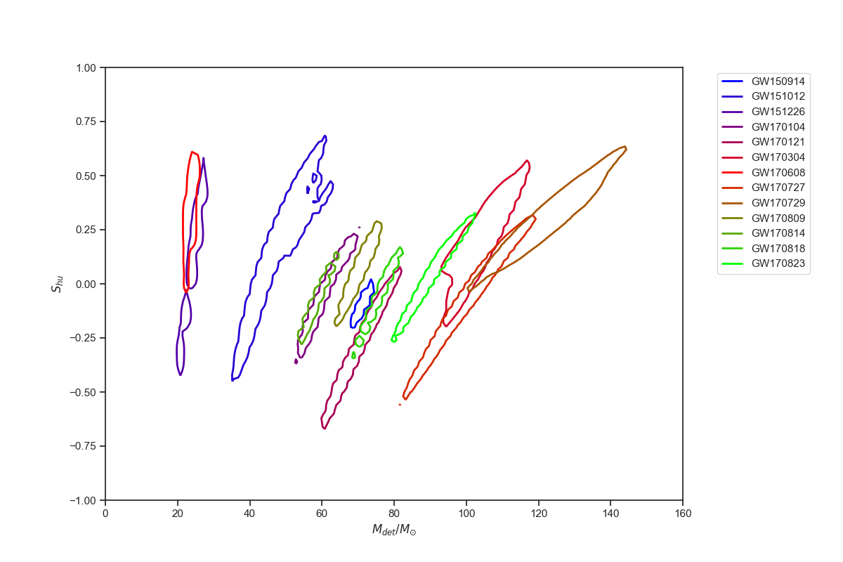
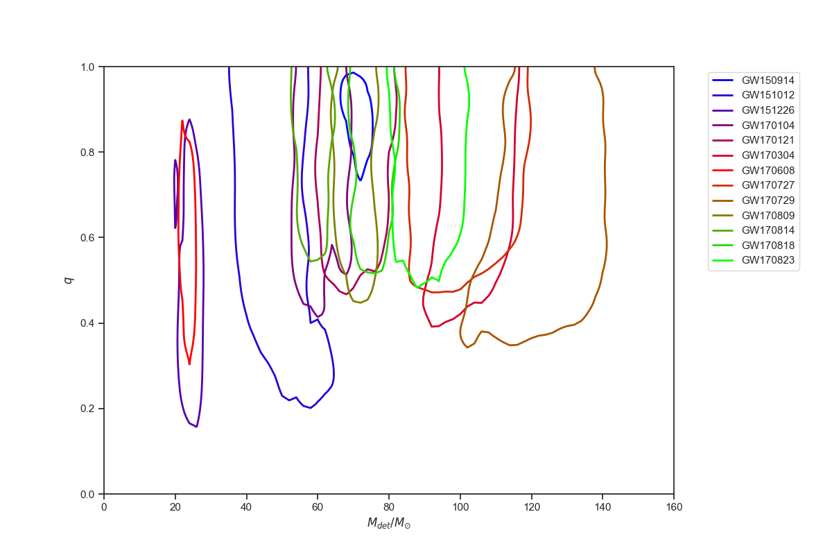
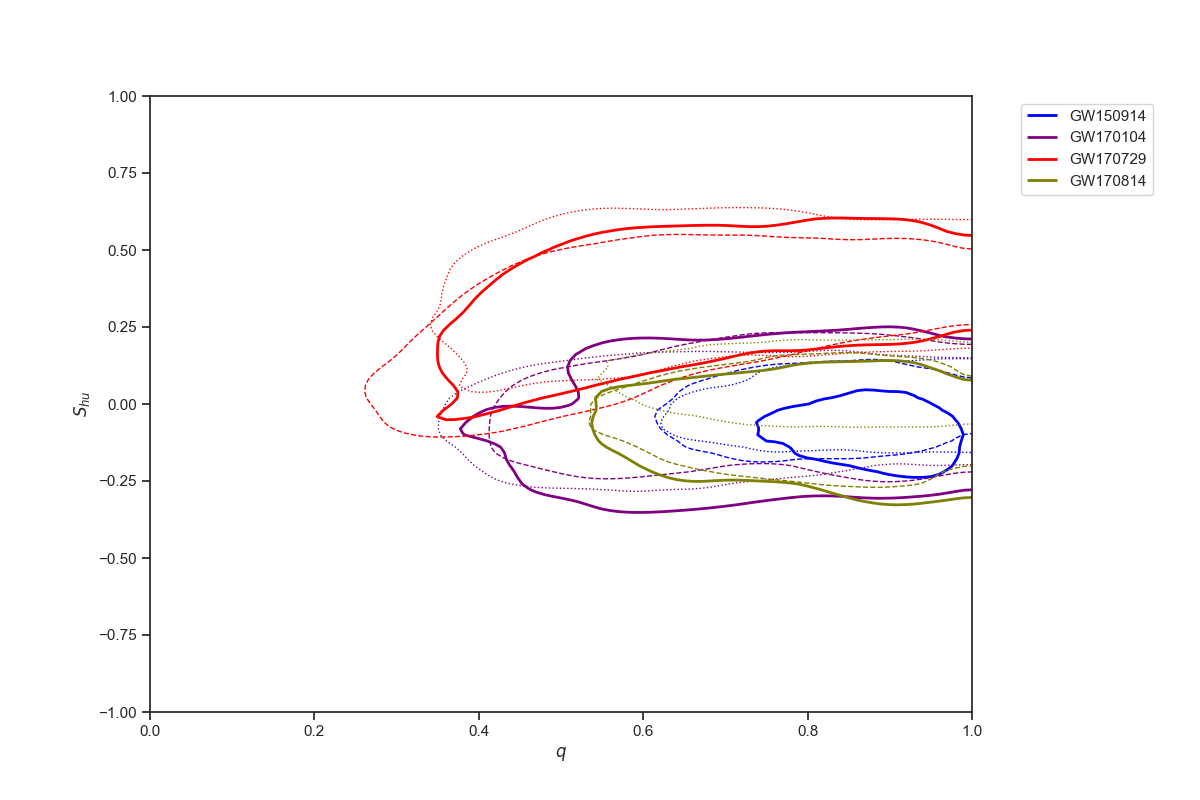
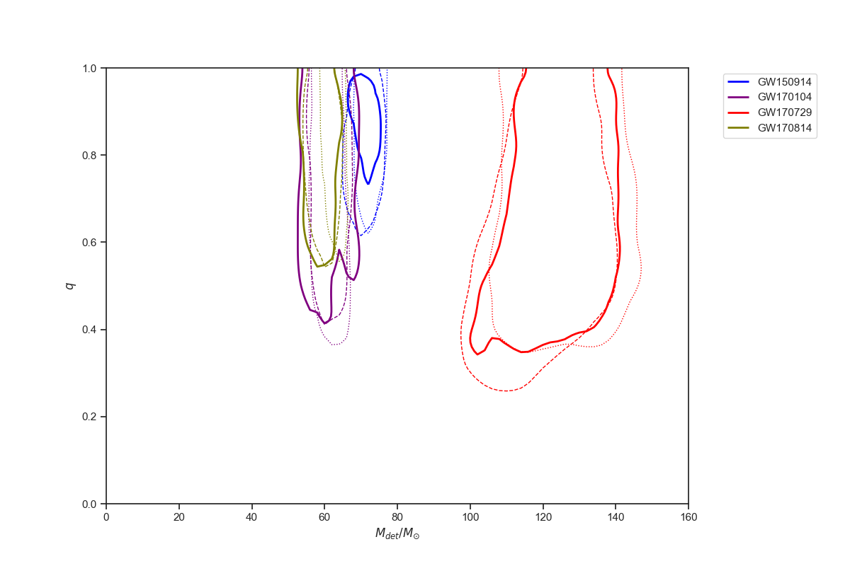
Figure 1 illustrates our inferences about binary masses and spin, using our preferred prior assumptions. Figure 2 shows the recovered mass and spin distributions for the four exemplary events in greater detail, for different prior choices, as well as previously-published fiducial LIGO results.

Figure 2: Comparison of inferred 90% credible intervals for selected binary black holes, using three different inference methods. Solid lines show our preferred results, as shown in Figure 1. Dotted lines show the corresponding bound obtained from the published, public fiducial GWTC-1 analyses of these events, which notably adopt a different prior than our fiducial results and which employ a mixture of approximations to general relativity. Dashed lines provide the corresponding bound from our analysis, after reanalyzing and adopting the same prior as used in GWTC-1. See Table 4 for a quantitative comparison between the marginal (one-dimensional) posteriors.

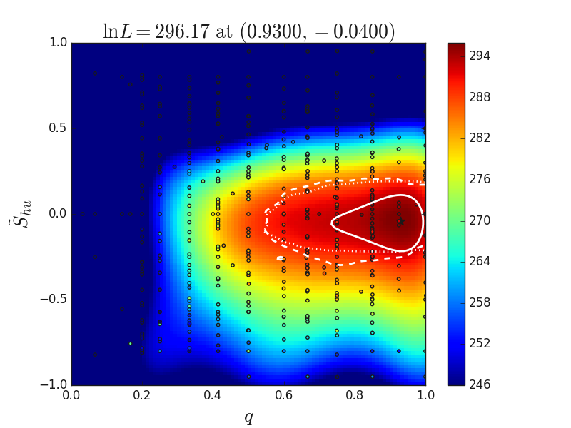
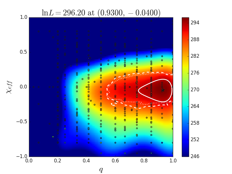
To illustrate the process of likelihood interpolation, we follow previous work Abbott et al. (2016e); Lovelace et al. (2016); Healy et al. (2019) and show the likelihood versus event parameters, superimposed with a (lower-dimensional, simplified) interpolated likelihood. We use GW150914 to illustrate our nonprecessing and precessing analyses’ likelihoods over the aligned and precessing binary spin parameters, relative to our grid of simulated binary black holes. The left panels of Figure 3 shows our interpolated marginal likelihood versus nonprecessing binary parameters. We emphasize the interpolation shown for illustration is performed only in two dimensions: for each simulation, we find the single largest value of $max_{M}{\cal L}(M,q,\chi_{1,z},\chi_{2,z})$, then use GPR to interpolate in $q$ and one spin degree of freedom, treating the other as a nuisance variable. This figure shows first that our simulation grid is quite dense relative to the support of the likelihood. The reconstructed likelihood varies smoothly over our parameter range. Second, this figure shows that, for our fiducial prior, marginal likelihood contours are in good agreement with our inferred posterior distribution. Third, the two left hand figures compare two different parameterizations for the dominant spin parameter: $\chi_{\rm eff}$ and $S_{hu}$. In this case, both produce consistent answers, showing the data prefers a narrow range of net aligned spins. Finally, the bottom right hand panel of Figure 3 shows a posterior corner plot. Each hexagon’s weight reflects the likelihood of parameters associated with that hexagon.

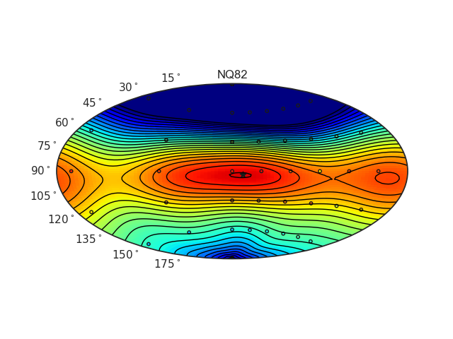
We also use GW190514 to illustrate our precessing analysis, using the 300 precessing single-spin simulations of the RIT catalog, again using a slightly simplified version of the analysis used for our tabulated results. The right panels of Figure 3 show slices through our parameter space corresponding to specific mass ratios and spin magnitudes. (This simulation catalog has only binaries where one spin has magnitude $|\bm{\chi}|=0.8$.) As above, for each simulation we select the largest value of $\ln{\cal L}$ for a specific simulation, maximizing over mass, and then interpolate this function over each two-dimensional slice. As expected from the purely aligned analysis, we find that the data disallows spins with significant components aligned or antialigned with the orbital angular momentum. Further, the best mass ratio slice in this simplified analysis corresponds to $q=0.82$, consistent with the purely aligned analysis. Despite exploring only one spin degree of freedom, we draw consistent conclusions about the precessing spin, which we can usefully compare to targeted studies with two precessing spin binaries.

Figure 2 shows the 90% credible intervals of our inferred posterior distribution for GW150914, using our fiducial assumptions (solid) and using the assumptions of GWTC-1 (dotted). For comparison, the dashed curves in this figure also show the GWTC-1 results. When adopting consistent priors, we obtain posterior distributions which are exceptionally consistent with previous work. With our fiducial prior, however, the inferred masses and spins differ. These differences are due to our preferred choice of priors, best illustrated in the bottom right hand panel of Figure 3.

Figure 3: Left panels: Comparative analysis of the $S_{hu}$ and $\chi_{eff}$ spins versus $q$ for GW150914 using the 477 nonprecessing binaries. The points show the parameters of these nonprecessing simulations. As described in the text, the color scale is based on an interpolation between each simulation’s maximum ${\cal L}$ (i.e., $\max_{M}{\cal L}(M,q,\chi_{1,z},\chi_{2,z})$) over (only) the two parameter dimensions shown in this plot. As in Figure 2, the contours are 90% credible intervals of a posterior based on our full 4-dimensional interpolated likelihood (solid); a reanalysis of the same likelihood, using conventional priors consistent with GWTC-1 (dashed); and the LIGO GWTC-1 analysis itself (dotted). Top right panel: Top likelihood panel for the binary spin orientation for GW150914 using the 300 precessing simulations. The star labels the most likely orientation of the spin and NQ82 label means a mass ratio $q=0.82$. Bottom right panel: Estimation of the (aligned) binary parameters $(M_{Total},q,\chi_{1},\chi_{2})$ for GW150914 using the 477 nonprecessing simulations. The weighted histogram is the posterior associated with the uniform priors. For comparison, we also superimpose the LIGO GWTC-1 posteriors in red, and the CIP analysis of the same dataset assuming the same priors as the LIGO GWTC-1 published results in green. The fiducial pseudo-precessing spin prior adopted by GWTC-1 strongly disfavors extreme positive or negative spins, relative to our fiducial uniform prior.

As seen in Figure 2, inferences about the other exemplary events’ masses and spins are less prior-dependent. For GW170814 and to a lesser extent GW170104, the posterior distributions’ 90% credible intervals are qualitatively and quantitatively quite similar. For GW170729, modest differences exist between our analysis and GWTC-1, which may reflect model systematics; see discussion in GWTC-1 The LIGO Scientific Collaboration et al. (2019) and elsewhere Chatziioannou et al. (2019); O’Shaughnessy and Lange (2019).

III.2 Discussion: Extrinsic parameters

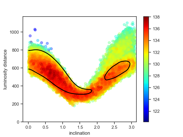
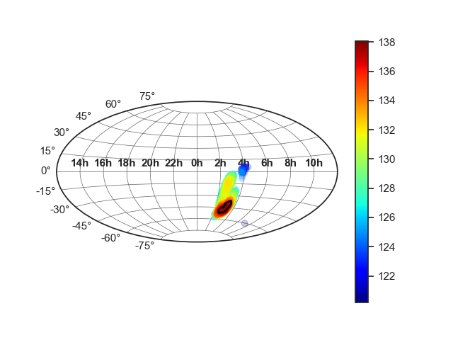
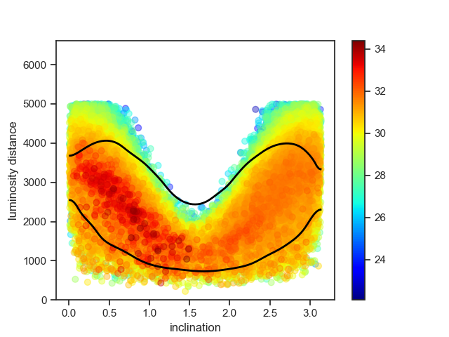
GW170814’s sky location was exceptionally tightly isolated via triple-coincident data. To illustrate our ability to also reconstruct binary extrinsic parameters, in Figure 4 we show the inferred 2d marginal distributions for distance-inclination (top panel) and sky location (bottom panel). The color scale shows our marginal distributions; the solid black line shows previously published results. We find good agreement, despite only using a very sparse set of simulations.

Figure 4: Sky localization on top and luminosity distance versus inclination angle of the binary on the bottom for GW170814. RIFT samples are colored by $\ln{L}$ and LIGO GWTC-1 posteriors are shown as solid black lines.

III.3 Discussion: Remnant properties

GW170729 was a massive binary black hole whose inferred net-aligned-spins ($\chi_{\rm eff}$ or $S_{hu}$ were likely significantly positive. As a result, its remnant properties are most different from the other merging black holes, with the largest remnant BH spin. Table 5 gives the final merged black hole properties and the peak frequency, luminosity and amplitude of the merger waveform. For those estimates we have used the nonprecessing 477 simulations and those values can be confronted with those given in Table III of the Ligo-Virgo Catalog Abbott et al. (2019) (given in the source frame). We observe again a large superposition of the 90% confidence intervals in all events. The results can also be confronted with the prediction from the remnant formulas given in Healy et al. (2014); Healy and Lousto (2017, 2018) where they use as an input the binary parameters given in Table 1.

Table 5: Parameter estimation of the final black hole mass, $m_{f}$, spin, $a_{f}$, and its recoil velocity, $v_{f}$, and the peak luminosity, $p_{L}$, waveform frequency $p_{O}$ at the maximum amplitude $p_{A}$ of the strain, at the mean of $\ln{\cal L}$ and its $90\%$ confidence ranges from the nonprecessing simulations.

Event	$m_{f}$	$a_{f}$	$v_{f}$	$10^{3}p_{L}$	$p_{O}$	$p_{A}$
GW150914	$0.9526^{+0.0030}_{-0.0035}$	$0.6788^{+0.0362}_{-0.0434}$	$215.5^{+181.1}_{-158.2}$	$0.974^{+0.083}_{-0.045}$	$0.3562^{+0.0087}_{-0.0089}$	$0.3928^{+0.0027}_{-0.0100}$
GW151012	$0.9508^{+0.0192}_{-0.0185}$	$0.7292^{+0.1376}_{-0.1696}$	$119.7^{+213.2}_{-101.6}$	$1.005^{+0.301}_{-0.480}$	$0.3681^{+0.0439}_{-0.0348}$	$0.3785^{+0.0250}_{-0.1273}$
GW151226	$0.9502^{+0.0201}_{-0.0202}$	$0.7264^{+0.1364}_{-0.2384}$	$135.6^{+212.0}_{-109.9}$	$0.959^{+0.343}_{-0.380}$	$0.3673^{+0.0423}_{-0.0452}$	$0.3763^{+0.0234}_{-0.0800}$
GW170104	$0.9525^{+0.0080}_{-0.0061}$	$0.6746^{+0.0644}_{-0.0996}$	$221.2^{+229.7}_{-201.4}$	$0.991^{+0.114}_{-0.173}$	$0.3543^{+0.0172}_{-0.0180}$	$0.3925^{+0.0060}_{-0.0305}$
GW170608	$0.9476^{+0.0162}_{-0.0193}$	$0.7468^{+0.1306}_{-0.1418}$	$104.0^{+151.0}_{-88.1}$	$1.106^{+0.254}_{-0.392}$	$0.3742^{+0.0444}_{-0.0333}$	$0.3790^{+0.0215}_{-0.0757}$
GW170729	$0.9430^{+0.0176}_{-0.0136}$	$0.8018^{+0.0610}_{-0.1284}$	$112.2^{+124.4}_{-86.2}$	$1.125^{+0.229}_{-0.373}$	$0.3838^{+0.0254}_{-0.0298}$	$0.3714^{+0.0252}_{-0.0504}$
GW170809	$0.9489^{+0.0111}_{-0.0058}$	$0.7172^{+0.0612}_{-0.1110}$	$197.3^{+188.0}_{-167.2}$	$1.061^{+0.097}_{-0.260}$	$0.3660^{+0.0139}_{-0.0227}$	$0.3901^{+0.0085}_{-0.0436}$
GW170814	$0.9553^{+0.0040}_{-0.0067}$	$0.6468^{+0.0700}_{-0.0492}$	$113.5^{+285.5}_{-87.4}$	$0.944^{+0.112}_{-0.056}$	$0.3502^{+0.0121}_{-0.0101}$	$0.3879^{+0.0083}_{-0.0130}$
GW170818	$0.9531^{+0.0082}_{-0.0080}$	$0.6750^{+0.0828}_{-0.1084}$	$149.0^{+263.7}_{-131.2}$	$0.987^{+0.129}_{-0.185}$	$0.3553^{+0.0188}_{-0.0206}$	$0.3910^{+0.0066}_{-0.0276}$
GW170823	$0.9512^{+0.0096}_{-0.0082}$	$0.6984^{+0.0792}_{-0.1172}$	$175.8^{+210.7}_{-144.4}$	$1.017^{+0.143}_{-0.212}$	$0.3610^{+0.0200}_{-0.0231}$	$0.3896^{+0.0075}_{-0.0364}$
GW170121	$0.9586^{+0.0078}_{-0.0075}$	$0.5950^{+0.1056}_{-0.1306}$	$155.1^{+231.4}_{-127.9}$	$0.885^{+0.136}_{-0.178}$	$0.3390^{+0.0218}_{-0.0220}$	$0.3897^{+0.0071}_{-0.0350}$
GW170304	$0.9470^{+0.0132}_{-0.0113}$	$0.7452^{+0.0844}_{-0.1286}$	$135.6^{+188.6}_{-109.4}$	$1.084^{+0.191}_{-0.287}$	$0.3724^{+0.0249}_{-0.0282}$	$0.3873^{+0.0103}_{-0.0490}$
GW170727	$0.9532^{+0.0108}_{-0.0101}$	$0.6748^{+0.1052}_{-0.1516}$	$172.5^{+214.9}_{-139.4}$	$0.976^{+0.179}_{-0.232}$	$0.3558^{+0.0253}_{-0.0289}$	$0.3890^{+0.0080}_{-0.0392}$

III.4 Contrasts with previously reported results

The figures and results emphasized above and derived from our fiducial priors are qualitatively similar but noticeably quantitatively different from previously-published results. However, as noted above, we have also performed all our calculations with the default priors adopted in previous work: uniform in $m_{1,z},m_{2,z}$ and compatible with spins which are isotropic and uniform in $|\bm{\chi}|$. Table 4 provides a quantitative comparison between our two sets of results (for nonprecessing binaries), and between our results and the analyses published in GWTC-1. Critically, this table shows that when we adopt similar priors to previous work, we find quite similar results, modulo a few exceptions. Though waveform systematics still plays some role, the principal difference between our inferences and previous work is our choice of prior assumptions.

As previously noted Abbott et al. (2016); The LIGO Scientific Collaboration et al. (2017b), the long-duration signals GW170608 and GW151226 are more challenging to analyze: few of our simulations have comparable duration,. Because we had to adopt a larger starting frequency $f_{\rm min}$, a pure NR analysis of these events is necessarily less tightly constraining than an analysis that could incorporate lower frequency information. As a result, for these two events we expect and observe more substantial differences between our inferences and inferences performed using longer-duration waveform models.

III.5 Events reported by external groups

In addition to the ten BBH GW events reported in the first LIGO and Virgo Gravitational-Wave Transient Catalog Abbott et al. (2019), there have been studies of other potentially astrophysical $(p_{astro}>0.98)$ events, such as (GW170121, GW170304, GW170727) reported in Venumadhav et al. (2020). Here we will apply our technique to have an independent parameter estimation of those events with highest claimed significance ($p_{astro}$). All inferred event parameters are described in the previously discussed Table 1 (aligned inferences), Table 2 (precessing inferences), and Table 6 (extrinsic parameters); all are consistent with the published results in Ref. Venumadhav et al. (2020), for instance for the estimated mass ratios $q$ and $\chi_{eff}$ and their 90% confidence intervals in all three signals. All analyses are performed using on-source PSDs. As a concrete example, we will discuss one event in greater detail: GW170304.

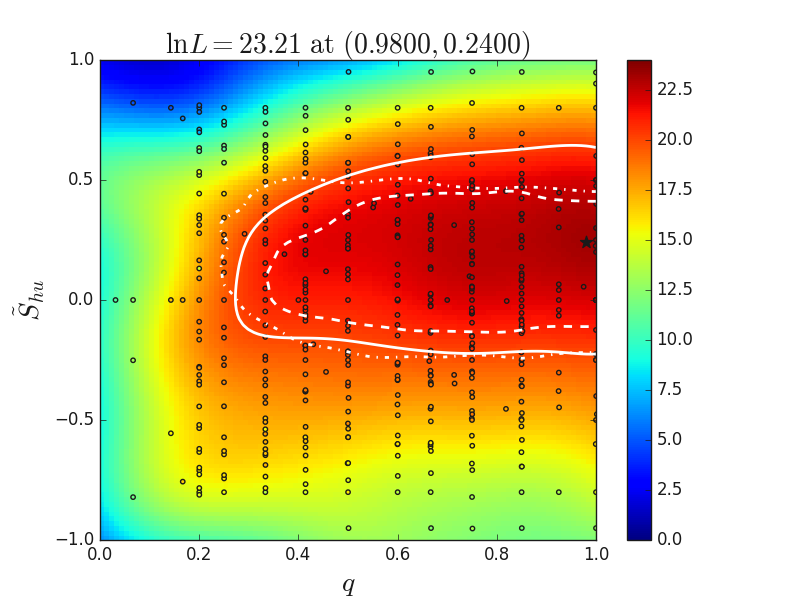
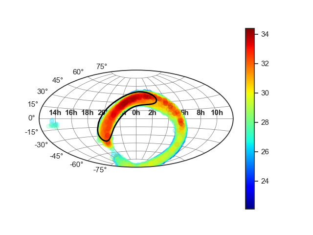
For these low-significance events, a large fraction of our simulation space is consistent with the observations for some mass scale, suggesting that systematics from simulation placement will be particularly small. Figure  5 illustrates the (peak) marginal likelihood for each simulation, versus $q$ and $S_{hu}$, as previously interpolated by a Gaussian process; compare to the corresponding Figure 3 for GW150914. For comparison, the heavy dashed line shows the inferred two-dimensional posterior distribution, using our fiducial prior as expected, its credible intervals are in good agreement with the marginal likelihood contours. Similarly, Figure  6 shows the recovered sky location and joint distance-inclination posterior for this event, using all the the simulations within the 90% confidence limit; for comparison, the black contour shows the published reconstructed sky location.

Figure 5: 90% Confidence level of the binary parameters for GW170304 in a two dimensional $(S_{hu},q)$, search (solid), CIP reanalysis (dashed), and published Princeton posterior (dash-dotted).

Figure 6: Sky localization on top and luminosity distance versus inclination angle of the binary on the bottom for GW170304. RIFT samples are colored by $\ln{L}$ and LIGO GWTC-1 posteriors are shown as solid black lines.

III.6 Waveform reconstructions

For each simulation in our catalog, we identify the optimal mass and extrinsic parameters, then generate a point estimate for the likely response of each detector. Table 6 provides the specific simulations (from the RIT catalog http://ccrg.rit.edu/~RITCatalog) and extrinsic parameters used to estimate the strain for each event. In Figure 7, we compare these point estimates to the whitened GW data in each interferometer, for all the events in GWTC-1; rows correspond to events, presented in chronological order. Examining these plots, this subtraction doesn’t seem to leave behind a notably significant or correlated residual for most events. As expected, for the two low-mass events, where our analysis is suboptimal due to limited simulation duration, some correlated high-frequency residual does remain near the merger epoch.

Table 6: Extrinsic parameters used to reconstruct the best fitting numerical relativity waveform in Fig. 7.

Event	Sim.	r.a.	decl	$\phi$	$\theta$	$\psi$	$D_{L}$	$z$
GW150914	RIT:BBH:0160	1.9298	-1.2710	4.4278	2.9828	1.8366	571.64	0.1188
GW151012	RIT:BBH:0040	3.9358	-0.0134	4.6488	1.3702	2.0121	516.54	0.1081
GW151226	RIT:BBH:0573	4.5194	-1.1913	3.5168	1.1708	1.8474	306.91	0.0661
GW170104	RIT:BBH:0162	2.1092	0.3889	3.0760	1.1386	1.3337	586.65	0.1217
GW170608	RIT:BBH:0555	2.1540	1.0300	5.7880	1.6134	0.7532	125.37	0.0277
GW170729	RIT:BBH:0015	5.2211	-0.8403	5.5634	0.8868	2.3039	2468.73	0.4345
GW170809	RIT:BBH:0204	0.2594	-0.5293	5.5287	2.6277	2.2101	1038.26	0.2047
GW170814	RIT:BBH:0661	0.8068	-0.8197	1.1063	0.2078	1.7285	635.37	0.1310
GW170818	RIT:BBH:0664	5.9577	0.3449	0.7399	2.0777	1.3192	562.29	0.1170
GW170823	RIT:BBH:0017	4.0601	-0.1352	1.1855	2.4861	3.0995	1653.22	0.3084

Figure 7: For each observed GW signal (rows) and each interferometer (columns), our best point estimate for the GW strain (solid red line in top panel); the whitened GW data (gray line); and the residual difference between the two (bottom panel). Table 6 provides the specific simulations and extrinsic parameters used to estimate the strain for each event.

III.7 Numerical Waveforms accuracy

In addition to the numerical convergence studies performed for our code, we have evaluated the impact our standard numerical resolutions have on the accuracy of our simulations for the first gravitational waves event GW150914 in Lovelace et al. (2016), where we performed comparative convergence studies of RIT waveforms with the completely independent numerical approach to solve the binary black hole problem by the SXS group. We have also performed those comparative studies for the first O2 event, GW170104 in Healy et al. (2018b). Both studies display convergence to each other’s approach with increasing numerical resolution and display that the lower resolutions used performs an excellent match to the signals.

Table 7: Variation of the maximum of $\ln{\cal L}$ with the numerical resolution of selected events. In the case of GW170823 an extrapolation of the result to infinite resolution (n$\to\infty$) and order of convergence of $\ln{\cal L}$.

Event	Simulation	low	medium	high	n$\to\infty$	order
GW170729	RIT:BBH:0166	36.78	36.58	36.59	–	–
GW170809	RIT:BBH:0198	58.46	58.47	58.44	–	–
GW170814	RIT:BBH:0062	148.18	148.22	148.23	–	–
GW170823	RIT:BBH:0113	57.32	57.77	58.03	58.66	2.25

Here we extend those analysis to several additional O2 events: GW170729, GW170809, GW170814, GW170823. We evaluate the maximum $\ln{\cal L}$ for a set of three numerical waveforms (see details of the simulations in Healy et al. (2017a, 2019)) with increasing resolution (typically those labeled with n100, n120, n140; see http://ccrg.rit.edu/~RITCatalog), and compare the results in Table 7. Those show that there is very little differences between low, medium, and high resolution runs regarding the evaluation of the likelihood and that even in the case of GW170823, where we find enough differences to extrapolate to infinite resolution, the extrapolated value lies within 1-sigma from the lowest resolution.

III.8 Null test

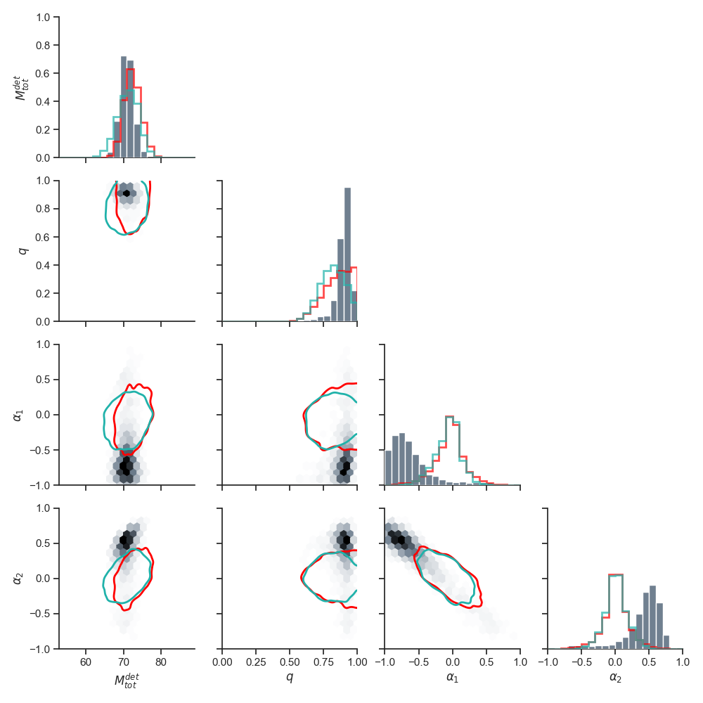
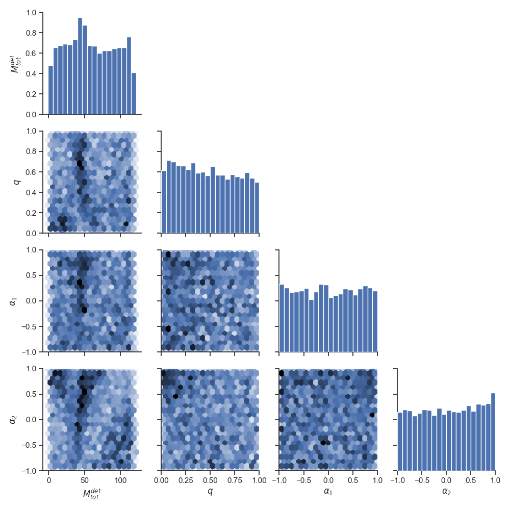
The specific finite set of simulation parameters in principle impacts the posterior distributions we recover. To assess this effect, we study a pure-noise signal as a control case. Figure 8 shows the parameters estimated for the BBH in the detector frame using 477 aligned spins simulations. The recovered posterior is consistent with our adopted prior, modulo small modulations principally in total binary mass.

Figure 8: Estimation of the (aligned) binary parameters $(M_{Total},q,\chi_{1},\chi_{2})$ for Null Test using the 477 nonprecessing simulations.

IV Conclusions and Discussion

The breakthroughs Pretorius (2005); Campanelli et al. (2006); Baker et al. (2006) in numerical relativity were instrumental in identifying the first detection of gravitational waves Abbott et al. (2016a) with the merger of two black holes. The comparison of different approaches to solve the binary black hole problem has produced an excellent agreement for the GW150914 Lovelace et al. (2016) and GW170104 Healy et al. (2018b), including higher (up to $\ell=5$) modes. We have shown in this paper that the use of numerical relativity waveform catalogs (See also Refs. Abbott et al. (2016e); Lange et al. (2017); Kumar et al. (2019)) allows the application of a consistent method for parameter estimation (of merging binary black holes) of the observed gravitational waves in the observation runs O1/O2. This method of direct comparison of the gravitational wave signals with numerical waveforms does not rely at all on any information from phenomenological models Babak et al. (2017); Hannam et al. (2014) (either Phenom or SEOBNR).

It also shows that with the current aligned spin coverage one can successfully carry out parameter estimations with results, at least as good as with contemporary phenomenological models Abbott et al. (2016a), particularly modulo uncertainty in priors. In particular, we included coverage of spins above 0.95 in magnitude up to mass ratios 2:1. Note that we have used a different set of priors, as discussed in Sec. III.4 but those differences display a measure of the uncertainties expected in the parameter estimations.

New forthcoming simulations (for instance targeted to followup any new detection or catalog expansions) will contribute to improve the binary parameter coverage, thus reducing the interpolation error. The next step will be to reduce the extrapolation error at very high spins by adding more simulations with spin magnitudes above 0.95. In addition, new simulations will extend the family displayed in Fig. 8 of Ref. Healy and Lousto (2020) with single spinning binaries to smaller mass ratios, i.e. $q<1/5$. Coverage for low total binary masses (below $20M_{\odot}$), in turn, would require longer full numerical simulations or hybridization of the current NR waveforms with post-Newtonian waveforms Sadiq et al. (2020).

The next area of development for the numerical relativity waveform catalogs is the coverage of precessing binaries. Those require expansion of the parameter space to seven dimensions (assuming negligible eccentricity), and is being carried out in a hierarchical approach by first neglecting the effects of the spin of the secondary black holes, which is a good assumption for small mass ratios. This approach has proven also successful when applied to all O1/O2 events. It required an homogeneous set of simulations since the differences in $\ln{\cal L}$ are subtle. In a second stage, a follow up of the first determined spin orientations can be performed with a two spin search. Another line of extension of the use of NR waveforms is its use in searches of GW (in addition to that of parameter estimation). A first implementation of the nonspinning waveforms (using for instance the simulations reported in Healy et al. (2017b)) would produce a prototype of this search analysis. The success of the current systematic study can be carried out to the next LIGO-Virgo observational run O3ab, and in particular to focus on studies of interesting gravitational waves events and perform targeted simulations to extract independent parameter estimations.