Light Field Compression by Residual CNN Assisted JPEG

Abstract

Light field (LF) imaging has gained significant attention due to its recent success in 3-dimensional (3D) displaying and rendering as well as augmented and virtual reality usage. Because of the two extra dimensions, LFs are much larger than conventional images. We develop a JPEG-assisted learning-based technique to reconstruct an LF from a JPEG bitstream with a bit per pixel ratio of 0.0047 on average. For compression, we keep the LF’s center view and use JPEG compression with 50% quality. Our reconstruction pipeline consists of a small JPEG enhancement network (JPEG-Hance), a depth estimation network (Depth-Net), followed by view synthesizing by warping the enhanced center view. Our pipeline is significantly faster than using video compression on pseudo-sequences extracted from an LF, both in compression and decompression, while maintaining effective performance. We show that with a 1% compression time cost and 18x speedup for decompression, our methods reconstructed LFs have better structural similarity index metric (SSIM) and comparable peak signal-to-noise ratio (PSNR) compared to the state-of-the-art video compression techniques used to compress LFs.

1 Introduction

Light fields (LF), as compared to conventional images, have two extra dimensions which represent angular information of the scene [1, 2, 3]. Hence, LFs contain a relatively large volume of data that makes storing and portability time consuming and costly. Also, decompression of LF video with a high angular resolution at acceptable frames per second (fps) for streaming is challenging. We aim to address these challenges by predicting the entire LF from its JPEG compressed center view.

Direct application of standard image compression techniques, such as JPEG, PNG, etclet@tokeneonedot, on an LF does not take advantage of existing redundancies between LF views. Video compression techniques, however, achieved better success in compressing LFs. To use video compression algorithms on LFs, a sequence of images is built from LF views, which is called pseudo-sequence[4]. A combination of machine learning (ML) methods, capable of predicting LF views, and video compression techniques was explored in [5]. In this work, we present a combination of JPEG compression with ML view predictions. LF synthesis techniques have shown the possibility of estimating the entire LF from a single view or a set of sparse views. Here, we show that there is enough information in the JPEG compressed center view—as well as a group of sub-aperture images (SAIs)—to predict the entire LF with a quality comparable to the use of the state of the art video compression techniques on the LF. We test the success of our method by comparing against state-of-the-art methods in LF compression that use the existing HEVC compression.

Our method is faster in compression and decompression by 100x and 10x, respectively, compared to the direct use of HEVC. This speed up means a set of 30 LFs with a spatial resolution of $(375,540)$ and angular resolution of $(7,7)$ can be decompressed on a typical gaming GPU in less than 0.02 seconds, while HEVC-based methods require more than 0.39 seconds. With increases in spatial or angular dimensions, HEVC-based methods reconstruction soon takes more than one second. Thus, streaming will not be possible without pre-decompression. Furthermore, while speeding up the process, we have maintained and, in most cases, improved the quality of reconstruction at the same bit per pixel (bpp) ratio. We have used the mean of peak signal-to-noise (MPSNR) ratio over all of the views and mean structural similarity index metric (MSSIM) to compare the reconstructed LFs of our model with those that use HEVC. We show that while the MPSNR of our method is comparable to the direct employment of HEVC, our model can achieve higher MSSIM. This results in fewer artifacts and better quality in the extracted synthetic aperture depth of field (DoF) images. Note that we built our model to be fully convolutional, thus, it can be used on LFs with any spatial resolution. Also, our model works in the RGB channel. This is an advantage compared to other techniques, which are using YUV channel, because most of the available LF datasets are in RGB and conversion between RGB and YUV is not lossless.

The contributions of this paper are as follows. We achieved compression speed-up of more than 100x and decompression speed-up of more than 10x compared to the use of HEVC on pseudo-sequences of LF views. At an average bpp of $.0047$, the LF’s DoF reconstructed with our method improved the SSIM by $0.31\%$ on average over the test dataset compared to the direct use of HEVC. Finally, we introduce a small, fast, and efficient convolutional neural network (CNN) for enhancing JPEG images for use in LFs. This network also boosts the SSIM of the final decompressed LF.

2 Related Work

2.1 Light Field View Synthesis

Linear view synthesis by Levin and Durand [6] and depth of field extension and super-resolution by Bishop and Favaro [7] are among the earliest works on LF view synthesis and reconstruction. Flynn et allet@tokeneonedot[8] proposed a deep learning method to predict novel views from a sequence of images with wide baselines. LF view synthesis became more popular after Kalantari et allet@tokeneonedot[9] showed in their work that an LF can be synthesized from its corner SAIs with high quality. Building on the work of Kalantari et allet@tokeneonedot, Yeung et allet@tokeneonedotused different sets of views to reconstruct dense LFs [10]. Srinivasan et allet@tokeneonedotdemonstrate the possibility of estimating the entire LF from its center view by extrapolating using machine learning methods [11]. Choi et allet@tokeneonedotextended the extrapolation to an LF taken with arrays of cameras [12]. LF fusion [13] and depth-guided techniques [14] have been popular in reconstructing an LF from a single or a sparse set of SAIs. Hu et allet@tokeneonedot[15] aimed for a faster LF reconstruction method by using hierarchical features fusion.

The backbone of nearly every view synthesis method enumerated here is the depth-map estimation. The current work is categorized as single view LF reconstruction. Our method is unique because we use a lossy compressed JPEG view from which to estimate the entire LF. We use residual learning methods to guess the possible artifacts from the JPEG compressed version of the center view to assist the main network for accurately estimating the depth map.

2.2 Light Field Compression

Lossless and lossy compression methods have been investigated extensively in the literature. For the lossless model, Perra [16] proposed an adaptive block differential prediction method and Helin et allet@tokeneonedot[17] described a sparse modeling with a predictive coding for SAIs of the LF.

The lossy models can be classified in to sub-categories of: i) standardized image/video compression techniques and ii) machine learning assisted compression techniques.

2.2.1 LF compression by standardized image/video compression methods

Standardized image and video compression techniques (especially HEVC) have been directly used to address the problem of the bulkiness of the LF, see e.g., [4, 18, 19]. Other methods, such as homography-based low-rank models [20] and Fourier disparity layers [21], have been used to reduce the angular dimension of the LF. In another work, the LF depth was segmented into 4D spatial-angular blocks, which were used for prediction, followed by encoding the residue using JPEG-2000 [22].

2.2.2 Machine learning assisted compression techniques

Followed by the breakthrough in synthesizing LF views from its four corners using CNN learning techniques introduced by [9], another work introduced a compression technique by using the same method and compressing the four corner views by HEVC [23]. In another work, the authors proposed to keep half of the views and encode them by HEVC and synthesize the other half by a CNN [5]. A CNN based epipolar plane image super-resolution algorithm was used in cooperation with HEVC to compress LF as well [24]. Wang et allet@tokeneonedotproposed a new LF video compression technique by deploying view synthesis methods from multiple inputs while encoding the input views by a proposed region-of-interest scheme [25]. Generative adversarial network based methods have been used in cooperation with video codec techniques to compress LF in [26, 27]. There has been multiple works on LF compression with use of standard video compression codecs in combination with learning based view synthesis [28, 29]. Unfortunately, we could not find any public version of these codes, or trained networks for the purpose of comparing our results with them. Hence, we have chosen the pseudo-sequence HEVC compression method for comparison because of its easy implementation and availability of the HEVC codec.

To the best of our knowledge, because the view extrapolation is ill posed, LF reconstruction from a lossy compressed single input (specifically, JPEG) has not been explored before our work.

2.3 JPEG Compression Artifact Reduction

For several decades, different researchers addressed the JPEG compression artifact reduction generally in three main groups: prior knowledge-based, filter-based, and learning-based approaches. Here though, we are interested in learning-based approaches. The basic intention of learning-based methods is to find a non-linear mapping between the JPEG compressed image—compressed at different compression ratios—to the ground truth uncompressed image. To the best of our knowledge, the first deep learning model to address this problem was created by Dong et allet@tokeneonedot[30], where they showed the possibility of enhancing the reconstructed JPEG image by a relatively shallow CNN. Since then, multiple researchers have gradually improved the performance of learning-based methods by introducing new networks such as: dual-domain representations [31], deep dual-domain based fast restoration [32], encoder-decoder networks with symmetric skip connection [33], CAS-CNN [34], one-to-one networks [35], DMCNN [36], and dual-stream multi-path recursive residual network [37]. While deeper networks and state of the art architectures have improved the task of JPEG artifact reduction, we are not focused solely on this task here. The ultimate goal of our JPEG-Hance network is to improve the estimated depth-map from the JPEG compressed center image of an LF. JPEG artifact reduction is the natural first step for extracting better depth-maps.

3 The Proposed Method

Here we describe our compression and decompression pipeline. The compression pipeline is simply extraction of the center view of the LF, compression by JPEG at 50% quality, followed by discarding of all other views. The decompression pipeline has the following steps:

1. JPEG decompression of the center view $c_{J}$

2. Enhancing $c_{J}$ by JPEG-Hance to $c_{E}$,

   $$c_{E}=J(c_{J}).$$ (1)

3. Estimating depth map $d(x,u)$ of every view $u$ from $c_{E}$,

   $$d=D(c_{E}).$$ (2)

4. Reconstructing LF by

   $$\mathit{L(x,u)}_{u_{0}\rightarrow u}=L(x+(u-u_{0})d(x,u),u_{0}),$$ (3)

   where $L$ is the approximated LF and $u_{0}$ is the middle view index. Variables $x$ and $u$ are spatial and angular indices.

3.1 Networks architectures

3.1.1 JPEG-Hance

The main goal of our JPEG-Hance network is to assist the Depth-Net in providing better depth map estimation. In doing so, it is certainly beneficial to improve the overall quality of the JPEG decompressed image by reducing the error between uncompressed ground truth images and the lossy compressed ones. However, the goal of our network is not general JPEG artifact reduction; instead, JPEG-Hance should learn to enhance the parts of the image which have the most effect on improving depth information extraction. To achieve this task, JPEG-Hance also needs to find correspondence information from the extracted depth maps. Therefore, it is trained in two phases: first, it learns to enhance any typical JPEG decompressed image, then again as part of the whole depth estimation pipeline. The architecture of JPEG-Hance is shown in Fig. 1. Inspired by ResNet50’s bottleneck building blocks structure [38], we have designed our JPEG-Hance as residual blocks. We added a batch normalization (BN) layer after each convolution followed by an exponential linear unit (ELU). The ELU followed by a last layer tanh seems to be the most promising activation pair of functions when dealing with regression of image data scaled to the interval $[-1,1]$.

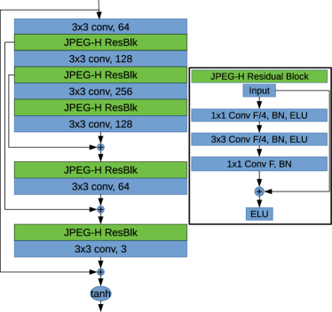
Figure 1: JPEG-Hance detailed structure

JPEG-Hance is pre-trained by minimizing the mean squared error of each pixel value in the RGB channels. Then it is added to the training pipeline for full reconstruction of LFs.

3.1.2 Depth-Net

Multiple images provide geometry information which can be used for LF reconstruction. A single image does not provide such information. Therefore, such information needs to be extracted by other methods. Machine learning techniques, particularly CNNs, showed a promising potential for estimating geometry from a single image [11, 9, 10]. Thus, for the problem of depth estimation from our enhanced center image, we use a residual CNN.

Our Depth-Net, depicted in Fig. 2, is responsible for estimating the depth map (disparity map) for all 49 views from the middle JPEG compressed view. Depth-net has three variants of residual blocks. The first variant is a down-sampler which uses a 2D convolution with strides of $(2\times 2)$, halving the spatial dimension of the input image. This block is used just before the first Depth Residual Block; each time the feature size is increased. The second type of block, the Depth Residual block, is the main residual block. This block is used the most and extracts most of the features. The structure of the Depth Residual block mimics the bottleneck structure of ResNet50 with added instance normalization after each of the first two convolution layers. Last, the Upsampler block is constructed to have a 2D deconvolution (transposed convolution) layer and two 2D convolution layers with kernel size of $(3\times 3)$. The deconvolution layer’s stride is set to $(2\times 2)$. These blocks are shown in Fig. 3.

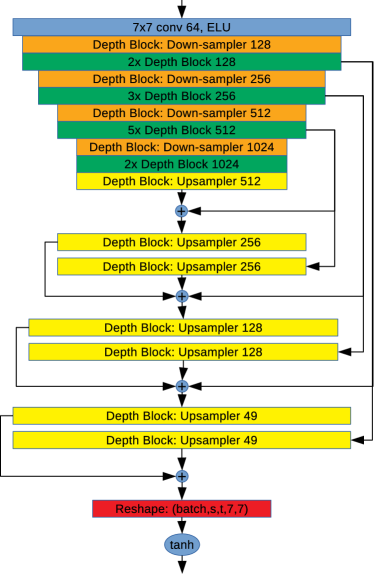
Figure 2: Depth-Net detailed structure

Figure 3: Depth-Net residual blocks

Because we are training the Depth-Net on the actual LF data and not the ground truth depth maps, our loss functions have to be designed to train the network in an unsupervised manner. Our Depth-net is predicting the LF’s depth while we do not have the ground truth depth to supervise the training. Thus, we define the Depth-Net pre-training loss function to be a weighted sum of four sub-functions: i) photometric loss $\mathit{L_{p}}$, ii) defocus loss $\mathit{L_{r}}$, iii) depth-consistency loss $\mathit{L_{c}}$, and iv) DoF loss $\mathit{L_{d}}$. The total loss is simply

$$\mathit{L}_{depth}=\alpha\mathit{L}_{p}+\alpha_{1}\mathit{L}_{r}+\alpha_{2}\mathit{L}_{c}+\alpha_{3}\mathit{L}_{d},$$ (4)

where $\alpha,\alpha_{1},\alpha_{2}$ and $\alpha_{3}$ are chosen to be $2$, $100$, $0.02$, and $10$ in our conducted experiments, which were empirically found to work well overall.

The image quality comparison sub-function $\psi$ [14] is constructed by combining mean absolute difference of pixels and image structural dissimilarity (DSSIM) that is derived from the structural similarity index metric (SSIM) [39]:

$$\psi(I_{1},I_{2})=\beta\frac{1-SSIM(I_{1},I_{2})}{2}+(1-\beta)\left\|I_{1}-I_{2}\right\|_{1},$$ (5)

where $I_{1},I_{2}$ are two images that are being compared and $\beta\in[0,1]$, which we empirically found that $0.15$ yields the best training results. Using the sub-function $\psi$, photometric loss is defined as [14]

$$L_{p}= \sum_{u}\big{[}\psi(L(x,u)_{u_{0}\rightarrow u},L(x,u))+$$

$$\psi(L(x,u)_{u\rightarrow u_{0}},L(x,u_{0}))\big{]}.$$ (6)

Because we are training an unsupervised Depth-Net, the more prior knowledge we can give the network, the better will be the training quality. Zhou et allet@tokeneonedot[14] introduced defocus cue loss

$$L_{d}=\psi\big{(}L(x,u_{0}),\frac{1}{N}\sum_{u}L(x,u)_{u\rightarrow u_{0}}\big{)}.$$ (7)

Also depth consistency (left-right or forward-backward) has been shown in the literature [40, 41, 42] to be a promising regularizer for LF view synthesis purpose, where

$$d_{u_{0}\rightarrow u}(x) =d_{u_{0}}\big{(}x,(u-u_{0})d(x,u)\big{)},$$ (8a)

$$L_{c} =\sum_{u}||d_{u}(x)-d_{u_{0}\rightarrow u}(x)||_{1}.$$ (8b)

Finally we have included depth of field (DoF) loss to further assist the network in learning depth information, where

$$DoF =\frac{1}{u}\sum_{u}L(x,u),$$ (9a)

$$L_{dof} =\psi\big{(}DoF,DoF_{u_{0}\rightarrow u}\big{)}.$$ (9b)

4 Experiments

In this section, we describe our method’s implementation details. Then, we use public data sets [11, 9] to evaluate our method and investigate the impact of different parts of our network on the performance of our model.

4.1 Data sets

We have conducted our experiments over the two public data sets: Flowers [11] and 30 Scenes [9]. Both of these data sets are captured by a Lytro Illum camera. The angular resolution of these data sets is $14\times 14$ views and the spatial resolution is variable between $375\times 540$ and $376\times 541$ pixels. The LF from these data sets are cropped to the size of $7\times 7\times 375\times 540$ to have a consistent size and vignetting.

4.2 Implementation details

Our pipeline was trained in multiple steps. We have implemented our model with Tensorflow 2.2 in python 3.7 on a workstation with an Intel Xeon W-2223 3.60 GHz, 64GB DDR4 memory, and NVIDIA Quadro RTX 5000.

4.2.1 JPEG-Hance

Our JPEG-Hance was pre-trained on the 30 Scenes training data set, which contains 100 scenes. The center views of these 100 scenes were extracted and used for training. In the training phase, the spatial dimensions of the JPEG-Hance were set to $128\times 128$. First a training pool of images with dimensions of $128\times 128$ was created by cropping the center views of the 100 scenes at 8 pixels steps. Therefore, the training pool had 150,000 different crops which we found sufficient for the JPEG-Hance network to be trained without over-fitting or under-fitting. The learning rate was set to 0.0004. The JPEG-Hance has a relatively small network: only 202,435 trainable parameters. The pre-training phase took about 90 minutes to converge.

4.2.2 Depth-Net

Our Depth-Net also has a pre-training step. The Depth-Net was pre-trained on the Flowers data set, which has 3,343 flowers. During the pre-training phase, the JPEG-Hance was used for enhancing center images while only Depth-Net parameters were trained. The input pipeline of the flowers contains random croppings to $128$ and data augmentation with 50% selection rate for the original data, 15% chance for random contrast change between $[0.1,0.5]$, 15% chance that the brightness was changed randomly up to $0.4\times$ original brightness, and the remaining 20% where the hue was randomly changed by up to $0.4\times$. During the pre-training phase, 16 random crops were extracted for each epoch, and the network was trained for 10 epochs. The learning rate was 0.0004. Depth-Net is the main network responsible for extracting the depth map; thus, it has more trainable parameters: about 38.2 million. The pre-training phase takes about 7 hours to converge.

A sample estimated depth is depicted in Fig. 4. This illustration demonstrates that the edges are not very sharp. This is because we have used the highly compressed lossy JPEG on center view, which adds blur to the edges, to estimate the disparity map. Thus, the resulting depth map is somewhat blurry.

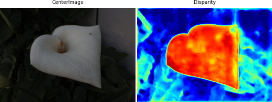
Figure 4: An estimated depth map. We can see that our network estimate is correct for most parts of the image. The map indicates that the flower is the nearest object to the LF camera and the leaves are just behind the flower and the wall is at the background, which is very realistic.

4.2.3 Training the entire pipeline

After pre-training the two networks, we can now train the entire pipeline. We add 100 scenes from the Flowers data set pool and use the same input pipeline as the one used for Depth-Net. The entire pipeline was trained for 45 epochs, gradually decreasing the learning rate from 0.0001 to 0.000001 for the last 5 epochs.

The last fine-tuning step includes training the pipeline on the data sets with input spatial dimensions of $375\times 540$. Here the augmentation selection is 25% original, 25% random contrast, 25% random brightness, and 25% random hue. Because of the structure of the Depth-Net network, the input images have to be zero-padded and the resulting LFs should be cropped to the correct size. The input dimension of the Depth-Net is $384\times 544$. The fine tuning phase takes 40 epochs for the network to converge with gradually decaying learning rate from 0.00005 to 0.000001. The fine-tuning phase took around 20 hours to converge, while all other pre-training phases took less than 10 hours cumulatively.

4.3 Performance comparison

We compared our compression-decompression results with a pseudo sequence method using the HEVC video compression Codec. We chose a raster sequence over spiral because raster had slightly better performance. The 30 scenes data set was used for comparing our method with HEVC. We use MSSIM and MPSNR metrics as well as SSIM and PSNR of the extracted DoF from LFs to compare the results, where

$$MSSIM =\frac{1}{M}\sum_{u}{SSIM(LF,\tilde{LF})},$$ (10)

$$MPSNR =\frac{1}{M}\sum_{u}{PSNR(LF,\tilde{LF})}.$$ (11)

To have a fair comparison, we tuned the QP factor of HEVC for each LF to reach approximately similar bpp between HEVC compressed LF and our method’s compressed representative. The average bpp for both methods on the 30 scenes data is $0.0047$. Fig. 5 shows that the LFs reconstructed by our method have very similar MPSNR and MSSIM to those decompressed by HEVC. By carefully examining Fig. 5 it is evident that, while our method outperforms HEVC in MSSIM, it is slightly inferior in MPSNR performance. Fig. 6 plots the PSNR and SSIM metrics for extracted DoFs from the reconstructed LFs. Here, our method meaningfully outperforms HEVC in SSIM metrics while further reducing the gap in PSNR. Because of this dual behavior in SSIM and PSNR metrics between our method’s results and HEVC’s, we have conducted experiment on the refocused images to find out which method is more reliable.

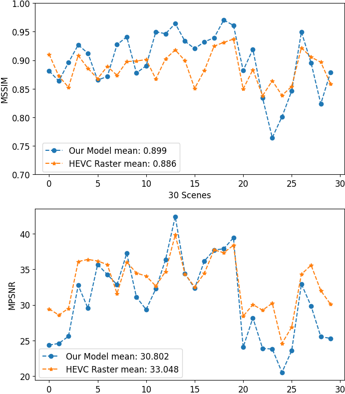
Figure 5: The top figure is showing the MSSIM for each reconstructed LF by our method and HEVC. The bottom figure is the MPSNR calculated for each reconstructed LF.

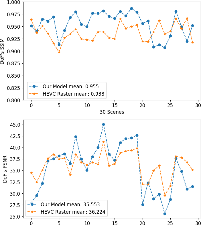
Figure 6: The DoF images extracted from ground truth LFs and the reconstructed LFs are compared using SSIM and PSNR metrics. The top plot is representing SSIM and the bottom one is showing PSNR for each LF in the 30 scenes.

The PSNR comparison between our model and HEVC over the test set for near and far focus in shown in Fig. 7. These results show that in some cases our model is superior and for other cases HEVC performs better. The mean PSNR of the HEVC for the test set is greater than ours by 1.3db for the near focus and 0.6db or the far focus. But for the case of the SSIM metric over the same test set, depicted in Fig. 8, we can see that in both near and far focuses, our model is performing better. Our model has 0.4% greater SSIM for near focus and 1.8% for far focus.

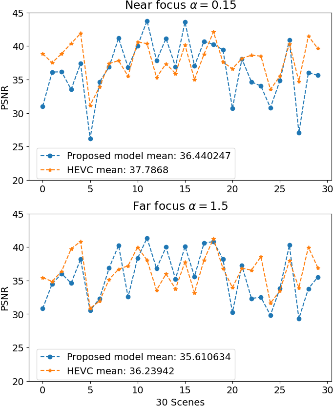
Figure 7: The reconstructed LFs from our model and HEVC is used to extract refocused images with refocusing parameters of $\alpha=0.15,1.5$, The top plot is showing the PSNR of the near focus images, and the bottom on is the far focus PSNRs.

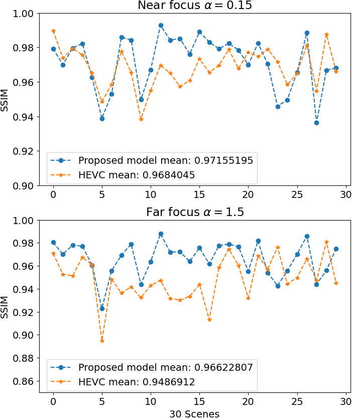
Figure 8: The SSIM of the near and far focus images extracted from HEVC and our proposed model is calculated and plotted.

While the quantitative results look nearly the same between our method and the HEVC compression technique, the reconstructed images show the real differences. Fig. 9 shows the reconstructed view of a statue from the LF. It is the 25th LF in the 30 Scenes data set. By looking at Fig. 6, we can see that HEVC’s MPSNR for this LF is more than 3dB greater than our model. Yet, Fig. 9 shows that the reconstructed LFs from our model are producing a visually better representation of the ground truth image. The HEVC reconstructed LF generally has more blur all over the image. This blur is, to some extent, caused by severe data loss. Fig. 10 illustrates another example, where the second leaf behind the front one is not reconstructed in HEVC decompressed LF. Last, we can see more details and better texture in the extracted DoF from our model, demonstrated in Fig. 11. In the refocused images extracted from our model, they have the same depth to the reference image and are refocused to the same focal plane as the ground truth. Images reconstructed from HEVC seem to lose the focal plane, especially in the one focused on the car in Fig. 9. Here, it becomes clear that our model is more successful in retaining the LF physical information. On the other hand, this finding indicates that the available quantitative metrics do not tell the whole story in comparing the two LF reconstruction methods. It is worth noting that for quality assessment, the SSIM metric is showing more agreement with the qualitative comparison than PSNR.

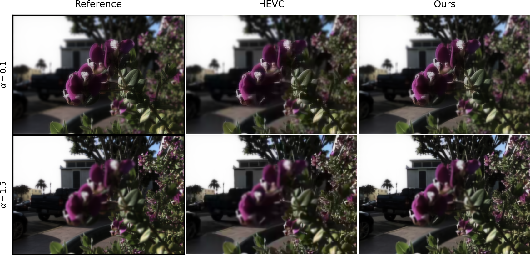
Figure 9: Two different focus points of an LF. The refocused DoFs in the top row are focused with $\alpha=0.1$ to the nearest flower, and the bottom row DoFs are focused at the car with $\alpha=1.5$. The images in the left most column are ground truth images. The middle column shows DoF images extracted from the HEVC reconstructed LF. The rightmost column contains the results from the LF reconstructed by our model.

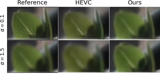
Figure 10: In this figure, a small slice from 9 shows HEVC loses more physical information compared to our model. The second leaf just behind the front leaf is not visible in the HEVC reconstructed LF’s DoF.

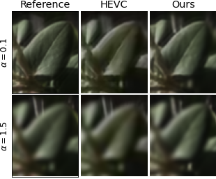
Figure 11: For better texture comparison, a small leaf from the 9 is magnified in this figure.

4.4 Speed Gain

Table 1 shows that the compression time of our proposed method is more than 100 times faster than that of HEVC, on the same computational hardware. This is because our compression pipeline is more efficient, which is just a JPEG algorithm on a fraction of the LF ($1/49$ in our case with 49 views). The HEVC algorithm processes all of the views.

Table 1: The time takes to compress all 30 LFs in the 30 scenes data set using our method and the HEVC. We can see an speed up of more than 102 times.

Method	CUDA	Comp time (s)
HEVC	No	43.53
JPEG-Hance + Depth-Net	No	0.42

For decompression, our method is 18 times faster than HEVC; see Table 2. To give a fair comparison, we used the NVIDIA optimized HEVC codec using the GPU’s video decoder. So on the same hardware, this will be the fastest implementation of HEVC.

Table 2: The reconstruction time on all LFs from the 30 scenes data set by our method and HEVC. We can see that our method is 18 times faster in decompressing.

Method	CUDA	Rec time (s)
HEVC	yes	0.399
JPEG-Hance + Depth-Net	yes	0.022

Overall, these results indicate that our model is suitable for compressing LF videos with high angular resolution. This is because our method can decompress in near real time inside the GPU without the barrier of transferring high volumes of data from host to GPU. The bandwidth used from host to GPU is equal to the size of only the center view of the LF.

5 Conclusions

We have designed a machine-learning assisted LF compression technique. It contains two sequential custom-designed CNNs: JPEG-Hance and Depth-Net. We showed that there is enough information in a highly compressed LF center view to estimate the depth-map of the LF and then use it to reconstruct the whole LF. Also, compression and decompression are faster with our method. We have used the public Flowers and 30 Scenes data sets to conduct our experiment and also to evaluate our model. We have achieved more than 100 times speedup during compression and about 18 times faster reconstruction compared to using HEVC on LF pseudo sequences. Comparing to HEVC, the reconstructed LFs using our method have superior MSSIMs, and they have comparable MPSNRs. Furthermore, the visual quality of the focal plane images reconstructed using our method are superior. For future work, we will try to add other views, with varied relative compression ratios, to further improve the quality of reconstruction. We will also explore options, such as improving the network architecture, other loss functions, larger training data sets, etclet@tokeneonedot, to enhance the MPSNR. We are also looking forward to deploying our method on an actual LF video to explore the achieved compression ratio and streaming capabilities.

References

- [1] Edward H Adelson, James R Bergen, et al. The plenoptic function and the elements of early vision, volume 2. Vision and Modeling Group, Media Laboratory, Massachusetts Institute of …, 1991.
- [2] Marc Levoy and Pat Hanrahan. Light field rendering. In Proceedings of the 23rd Annual Conference on Computer Graphics and Interactive Techniques, SIGGRAPH ’96, page 31–42, New York, NY, USA, 1996. Association for Computing Machinery.
- [3] Ren Ng, Marc Levoy, Mathieu Brédif, Gene Duval, Mark Horowitz, and Pat Hanrahan. Light Field Photography with a Hand-held Plenoptic Camera. Research Report CSTR 2005-02, Stanford university, April 2005.
- [4] D. Liu, L. Wang, L. Li, Zhiwei Xiong, Feng Wu, and Wenjun Zeng. Pseudo-sequence-based light field image compression. In 2016 IEEE International Conference on Multimedia Expo Workshops (ICMEW), pages 1–4, 2016.
- [5] Z. Zhao, S. Wang, C. Jia, X. Zhang, S. Ma, and J. Yang. Light field image compression based on deep learning. In 2018 IEEE International Conference on Multimedia and Expo (ICME), pages 1–6, 2018.
- [6] A. Levin and F. Durand. Linear view synthesis using a dimensionality gap light field prior. In 2010 IEEE Computer Society Conference on Computer Vision and Pattern Recognition, pages 1831–1838, 2010.
- [7] T. E. Bishop and P. Favaro. The light field camera: Extended depth of field, aliasing, and superresolution. IEEE Transactions on Pattern Analysis and Machine Intelligence, 34(5):972–986, 2012.
- [8] John Flynn, Ivan Neulander, James Philbin, and Noah Snavely. Deepstereo: Learning to predict new views from the world’s imagery. In Proceedings of the IEEE Conference on Computer Vision and Pattern Recognition (CVPR), June 2016.
- [9] Nima Khademi Kalantari, Ting-Chun Wang, and Ravi Ramamoorthi. Learning-based view synthesis for light field cameras. ACM Trans. Graph., 35(6), November 2016.
- [10] Henry Wing Fung Yeung, Junhui Hou, Jie Chen, Yuk Ying Chung, and Xiaoming Chen. Fast light field reconstruction with deep coarse-to-fine modeling of spatial-angular clues. In The European Conference on Computer Vision (ECCV), September 2018.
- [11] Pratul P. Srinivasan, Tongzhou Wang, Ashwin Sreelal, Ravi Ramamoorthi, and Ren Ng. Learning to synthesize a 4d rgbd light field from a single image. In The IEEE International Conference on Computer Vision (ICCV), Oct 2017.
- [12] Inchang Choi, Orazio Gallo, Alejandro Troccoli, Min H. Kim, and Jan Kautz. Extreme view synthesis. In The IEEE International Conference on Computer Vision (ICCV), October 2019.
- [13] Ben Mildenhall, Pratul P. Srinivasan, Rodrigo Ortiz-Cayon, Nima Khademi Kalantari, Ravi Ramamoorthi, Ren Ng, and Abhishek Kar. Local light field fusion: Practical view synthesis with prescriptive sampling guidelines. ACM Trans. Graph., 38(4), July 2019.
- [14] Wenhui Zhou, Gaomin Liu, Jiangwei Shi, Hua Zhang, and Guojun Dai. Depth-guided view synthesis for light field reconstruction from a single image. Image and Vision Computing, 95:103874, 2020.
- [15] Zexi Hu, Yuk Ying Chung, Wanli Ouyang, Xiaoming Chen, and Zhibo Chen. Light field reconstruction using hierarchical features fusion. Expert Systems with Applications, 151:113394, 2020.
- [16] Cristian Perra. Lossless plenoptic image compression using adaptive block differential prediction. In 2015 IEEE International Conference on Acoustics, Speech and Signal Processing (ICASSP), pages 1231–1234. IEEE, 2015.
- [17] Petri Helin, Pekka Astola, Bhaskar Rao, and Ioan Tabus. Sparse modelling and predictive coding of subaperture images for lossless plenoptic image compression. In 2016 3DTV-Conference: The True Vision-Capture, Transmission and Display of 3D Video (3DTV-CON), pages 1–4. IEEE, 2016.
- [18] C. Conti, P. Nunes, and L. D. Soares. Hevc-based light field image coding with bi-predicted self-similarity compensation. In 2016 IEEE International Conference on Multimedia Expo Workshops (ICMEW), pages 1–4, 2016.
- [19] Y. Li, R. Olsson, and M. Sjöström. Compression of unfocused plenoptic images using a displacement intra prediction. In 2016 IEEE International Conference on Multimedia Expo Workshops (ICMEW), pages 1–4, 2016.
- [20] X. Jiang, M. Le Pendu, R. A. Farrugia, and C. Guillemot. Light field compression with homography-based low-rank approximation. IEEE Journal of Selected Topics in Signal Processing, 11(7):1132–1145, 2017.
- [21] E. Dib, M. L. Pendu, and C. Guillemot. Light field compression using fourier disparity layers. In 2019 IEEE International Conference on Image Processing (ICIP), pages 3751–3755, 2019.
- [22] I. Tabus, P. Helin, and P. Astola. Lossy compression of lenslet images from plenoptic cameras combining sparse predictive coding and jpeg 2000. In 2017 IEEE International Conference on Image Processing (ICIP), pages 4567–4571, 2017.
- [23] M. Le Pendu X. Jiang and C. Guillemot. Light field compression using depth image based view synthesis. In 2017 IEEE International Conference on Multimedia Expo Workshops (ICMEW), pages 19–24, 2016.
- [24] J. Zhao, P. An, X. Huang, L. Shan, and R. Ma. Light field image sparse coding via cnn-based epi super-resolution. In 2018 IEEE Visual Communications and Image Processing (VCIP), pages 1–4, 2018.
- [25] B. Wang, Q. Peng, E. Wang, K. Han, and W. Xiang. Region-of-interest compression and view synthesis for light field video streaming. IEEE Access, 7:41183–41192, 2019.
- [26] C. Jia, X. Zhang, S. Wang, S. Wang, and S. Ma. Light field image compression using generative adversarial network-based view synthesis. IEEE Journal on Emerging and Selected Topics in Circuits and Systems, 9(1):177–189, 2019.
- [27] Deyang Liu, Xinpeng Huang, Wenfa Zhan, Liefu Ai, Xin Zheng, and Shulin Cheng. View synthesis-based light field image compression using a generative adversarial network. Information Sciences, 545:118 – 131, 2021.
- [28] J. Hou, J. Chen, and L. Chau. Light field image compression based on bi-level view compensation with rate-distortion optimization. IEEE Transactions on Circuits and Systems for Video Technology, 29(2):517–530, 2019.
- [29] J. Wang, Q. Wang, R. Xiong, Q. Zhu, and B. Yin. Light field image compression using multi-branch spatial transformer networks based view synthesis. In 2020 Data Compression Conference (DCC), pages 397–397, 2020.
- [30] Chao Dong, Yubin Deng, Chen Change Loy, and Xiaoou Tang. Compression artifacts reduction by a deep convolutional network. In The IEEE International Conference on Computer Vision (ICCV), December 2015.
- [31] Jun Guo and Hongyang Chao. Building dual-domain representations for compression artifacts reduction. In Bastian Leibe, Jiri Matas, Nicu Sebe, and Max Welling, editors, Computer Vision – ECCV 2016, pages 628–644, Cham, 2016. Springer International Publishing.
- [32] Zhangyang Wang, Ding Liu, Shiyu Chang, Qing Ling, Yingzhen Yang, and Thomas S. Huang. D3: Deep dual-domain based fast restoration of jpeg-compressed images. In The IEEE Conference on Computer Vision and Pattern Recognition (CVPR), June 2016.
- [33] Xiaojiao Mao, Chunhua Shen, and Yu-Bin Yang. Image restoration using very deep convolutional encoder-decoder networks with symmetric skip connections. In D. D. Lee, M. Sugiyama, U. V. Luxburg, I. Guyon, and R. Garnett, editors, Advances in Neural Information Processing Systems 29, pages 2802–2810. Curran Associates, Inc., 2016.
- [34] L. Cavigelli, P. Hager, and L. Benini. Cas-cnn: A deep convolutional neural network for image compression artifact suppression. In 2017 International Joint Conference on Neural Networks (IJCNN), pages 752–759, 2017.
- [35] Baochang Zhang, Jiaxin Gu, Chen Chen, Jungong Han, Xiangbo Su, Xianbin Cao, and Jianzhuang Liu. One-two-one networks for compression artifacts reduction in remote sensing. ISPRS Journal of Photogrammetry and Remote Sensing, 145:184 – 196, 2018. Deep Learning RS Data.
- [36] X. Zhang, W. Yang, Y. Hu, and J. Liu. Dmcnn: Dual-domain multi-scale convolutional neural network for compression artifacts removal. In 2018 25th IEEE International Conference on Image Processing (ICIP), pages 390–394, 2018.
- [37] Z. Jin, M. Z. Iqbal, W. Zou, X. Li, and E. Steinbach. Dual-stream multi-path recursive residual network for jpeg image compression artifacts reduction. IEEE Transactions on Circuits and Systems for Video Technology, pages 1–1, 2020.
- [38] Kaiming He, Xiangyu Zhang, Shaoqing Ren, and Jian Sun. Deep residual learning for image recognition. In Proceedings of the IEEE Conference on Computer Vision and Pattern Recognition (CVPR), June 2016.
- [39] Zhou Wang, A. C. Bovik, H. R. Sheikh, and E. P. Simoncelli. Image quality assessment: from error visibility to structural similarity. IEEE Transactions on Image Processing, 13(4):600–612, 2004.
- [40] Clement Godard, Oisin Mac Aodha, and Gabriel J. Brostow. Unsupervised monocular depth estimation with left-right consistency. In Proceedings of the IEEE Conference on Computer Vision and Pattern Recognition (CVPR), July 2017.
- [41] Yang Wang, Yi Yang, Zhenheng Yang, Liang Zhao, Peng Wang, and Wei Xu. Occlusion aware unsupervised learning of optical flow. In Proceedings of the IEEE Conference on Computer Vision and Pattern Recognition (CVPR), June 2018.
- [42] Zhichao Yin and Jianping Shi. Geonet: Unsupervised learning of dense depth, optical flow and camera pose. In Proceedings of the IEEE Conference on Computer Vision and Pattern Recognition (CVPR), June 2018.