Automatic Variationally Stable Analysis for Finite Element Computations: Transient Convection-Diffusion Problems

Abstract

We present an application of stable finite element (FE) approximations of convection-diffusion initial boundary value problems (IBVPs) using a weighted least squares FE method, the automatic variationally stable finite element (AVS-FE) method [1]. The transient convection-diffusion problem leads to issues in classical FE methods as the differential operator can be considered a singular perturbation in both space and time. The stability property of the AVS-FE method, allows us significant flexibility in the construction of FE approximations in both space and time. Thus, in this paper, we take two distinct approaches to the FE discretization of the convection-diffusion problem: $i)$ considering a space-time approach in which the temporal discretization is established using finite elements, and $ii)$ a method of lines approach in which we employ the AVS-FE method in space whereas the temporal domain is discretized using the generalized-$\alpha$ method. We also consider another space-time technique in which the temporal direction is partitioned, thereby leading to finite space-time ”slices” in an attempt to reduce the computational cost of the space-time discretizations.

We present numerical verifications for these approaches, including numerical asymptotic convergence studies highlighting optimal convergence properties. Furthermore, in the spirit of the discontinuous Petrov-Galerkin (DPG) method by Demkowicz and Gopalakrishnan [2, 3, 4, 5, 6], the AVS-FE method also leads to readily available a posteriori error estimates through a Riesz representer of the residual of the AVS-FE approximations. Hence, the norm of the resulting local restrictions of these estimates serve as error indicators in both space and time for which we present multiple numerical verifications in mesh adaptive strategies.

1 Introduction

Transient BVPs are commonplace in engineering applications and to date still pose significant challenges in numerical analysis and numerical modeling. Time dependency in many BVPs, such as the heat equation, involve partial derivatives of the trial variable with respect to time and leads to numerical instabilities unless careful considerations are taken. The reason being that the time derivative is a convective transport term, i.e., transient problems may lead to unstable discretizations, particularly in the FE context. Additionally, the target problem of convection-diffusion also result in numerical instabilities in its spatial discretizations which lead to the development of the AVS-FE method in [1]. To overcome the stability issues in both space and time we propose two distinct approaches employing the AVS-FE method. First, we take a space-time approach in which space and time are discretized directly considering time an additional dimension using the AVS-FE method. Second, we consider a method of lines to decouple the computations in space and time and employ a generalized $\alpha$ method for the temporal discretization [7, 8, 9].

The use of space-time FE methods remains attractive as the approximations are standard FE approximations and therefore inherit attractive features of FE methods such as a priori and a posteriori error estimation and mesh adaptive strategies. Examples of space-time FE methods can be found in, e.g., [10, 11, 12]. The AVS-FE method [1] being stable for any differential operator is therefore a prime candidate for space-time FE discretizations. Its stability property is a consequence of the philosophy of the DPG method in which the test space consist of functions that are computed on-the-fly from Riesz representation problems [2, 3, 4, 5, 6]. In [13], the AVS-FE method is successfully employed in space and time for the Cahn-Hilliard BVP. The goal here was the extension of the AVS-FE method to a nonlinear BVP as well as an initial verification of AVS-FE space-time solutions. Similarly, in [14], the AVS-FE method is employed for space time solutions of a nonlinear transient wave propagation problem, the Korteweg de-Vries equation. Furthermore, its built-in a posteriori error estimate and their corresponding error indicators can be directly applied to drive adaptivity. The DPG method has been successfully applied to several transient problems, e.g., convection-diffusion and the Navier-Stokes equations [15, 16, 17]. These space-time formulations are available in the DPG FE code Camellia of Nathan Roberts [18]. Recent efforts in DPG methods for transient problems include the use of optimal testing in time, see e.g., [19, 20]

Alternatively, the method of lines can be employed to decouple the discretization of space and time where the spatial dimension is discretized to obtain a semi-discrete system. Then, using a time integrator, the discretization of the temporal domain subsequently results in a fully discrete system of equations. Here, we employ the AVS-FE method in space and the generalized-$\alpha$ method in time. Chung and Hulbert introduced the generalized-$\alpha$ method in [9] to solve hyperbolic problems and extended it to parabolic differential equations such as Navier-Stokes equations in [21]. The method provides second-order accuracy in the temporal domain as well as unconditional stability. Although the method allows us to control the numerical dissipation in the high-frequency regions, it delivers adequately accurate results in low-frequency domains. Introduction of a user-defined parameter provides this control and includes the HHT-$\alpha$ method of Hilber, Hughes, Taylor [22] and the WBZ-$\alpha$ method of Wood, Bossak, and Zienkiewicz [23].

In the following, we introduce the AVS-FE method for transient BVPs by taking the two distinct approaches introduced above. In Section 2 we introduce our model problem and notations in addition to a review of the AVS-FE methodology and present the AVS-FE weak formulation to be used. In this section we also present the discretization of the weak form, an alternative saddle point structure of the AVS-FE method, and its built-in a posteriori error estimate. In Section 3 we present the time discretization techniques: the method of lines using AVS-FE method in space and generalized-$\alpha$ method in time is presented in Section 3.1; and the space-time AVS-FE method in Section 3.2. Results from numerical verifications for numerous PDEs and applications are presented in Section 4. Finally, we draw conclusions and discuss potential directions of future work in Section 5.

2 The AVS-FE Methodology

The AVS-FE method [1] allows us to compute stable FE approximations to BVPs for any differential operator, provided its kernel is trivial and the computations of optimal test functions is sufficiently accurate. In this section we introduce our model problem and briefly review the AVS-FE method, a thorough introduction can be found in [1].

2.1 Model Problem and Notation

Let $\Omega\subset\mathbb{R}^{N}$, $N\leq 2$ be an open bounded domain with Lipschitz boundary $\partial\Omega$ and outward unit normal vector $\mathbf{n}$, and let $T$ be the final time. Then, define $\Omega_{T}=\Omega\times(0,T)$ to be the space time domain which is open and bounded with a Lipschitz boundary $\partial\Omega_{T}=\overline{\Gamma_{in}\cup\Gamma_{out}\cup\Gamma_{0}\cup\Gamma_{T}}$. $\Gamma_{in}$ and $\Gamma_{out}$ are the in and outflow boundaries, respectively, and $\Gamma_{0}$ and $\Gamma_{T}$ are the initial and final time boundaries, respectively. The transient model problem is therefore the following linear convection-diffusion IBVP:

$$\boxed{\begin{array}[]{l}\text{Find }u\text{ such that:}\\[3.61371pt] \qquad\begin{array}[]{rcl}\displaystyle\frac{\partial u}{\partial t}-\bm{\nabla}\cdot(\epsilon\bm{\nabla}u)\,+\,{\mathbf{b}}\cdot\bm{\nabla}u&=&f,\quad\text{ in }\,\Omega_{T},\\[3.61371pt] \qquad u&=&u_{in},\quad\text{ on }\,\Gamma_{in},\\ \qquad\epsilon\bm{\nabla}u\cdot\mathbf{n}&=&g,\quad\text{ on }\,\Gamma_{out},\\ \qquad u&=&u_{0},\quad\text{ on }\,\Gamma_{0},\end{array}\end{array}}$$ (1)

where $\epsilon\in L^{\infty}(\Omega)$ denotes the isotropic diffusion parameter; ${\mathbf{b}}\in[L^{2}(\Omega)]^{2}$ the convection coefficient; $f\in L^{2}(\Omega)$ the source function; and $g\in H^{-1/2}(\Gamma_{out})$ the Neumann boundary data. Note that the gradient operator $\bm{\nabla}$ refers to the spatial gradient operator, e.g., $\bm{\nabla}(\cdot)=\{\frac{\partial(\cdot)}{\partial x},\frac{\partial(\cdot)}{\partial y}\}^{\text{T}}$.

2.2 Weak Formulation and FE Discretization

We omit the full derivation of the weak formulation here and mention key points only. The derivation of a weak formulation for the AVS-FE method is shown in, e.g. [1]. To establish a weak formulation of (1), we need a regular partition $\mathcal{P}_{h}$ of $\Omega_{T}$ into elements $K_{m}$, such that:

$$\Omega_{T}=\text{int}(\bigcup_{K_{m}\in\mathcal{P}_{h}}\overline{K_{m}}).$$

We introduce a flux variable $\mathbf{q}=\epsilon\bm{\nabla}u$, and recast (1) as a system of (distributional) first-order PDEs:

$$\boxed{\begin{array}[]{l}\text{Find }(u,\mathbf{q})\in H^{1}(\Omega_{T})\times(H(\text{div},\Omega)\times L^{2}(0,T))\text{ such that:}\\[3.61371pt] \qquad\begin{array}[]{rcl}\displaystyle\bm{\nabla}u-\frac{1}{\epsilon}\mathbf{q}&=&0,\quad\text{ in }\,\Omega_{T},\\ \displaystyle\frac{\partial u}{\partial t}-\bm{\nabla}\cdot\mathbf{q}\,+\,{\mathbf{b}}\cdot\bm{\nabla}u&=&f,\quad\text{ in }\,\Omega_{T},\\[1.8063pt] \qquad u&=&u_{in},\quad\text{ on }\,\Gamma_{in},\\ \qquad\mathbf{q}\cdot\mathbf{n}&=&g,\quad\text{ on }\,\Gamma_{out},\\ \qquad u&=&u_{0},\quad\text{ on }\,\Gamma_{0}.\end{array}\end{array}}$$ (2)

Note that the flux variable $\mathbf{q}$ depends on time but only has the same number of components as the dimension of $\Omega$ and in the weak enforcement of the PDE, it belongs to $H(\text{div},\Omega)\times L^{2}(0,T)$. To make notation more compact in the following, we write $H(\text{div},\Omega)$ for $H(\text{div},\Omega)\times L^{2}(0,T)$, and analogously for its broken counterpart.

To derive the AVS-FE weak formulation, we enforce the PDEs (2) weakly on each element $K_{m}\in\mathcal{P}_{h}$, apply integration by parts to shift all derivatives to the test functions except the time derivative. After subsequent summation of the local contributions we arrive at the global variational formulation:

$$\boxed{\begin{array}[]{ll}\text{Find }(u,\mathbf{q})\in U(\Omega_{T})&\text{ such that:}\\[3.61371pt] &\quad B((u,\mathbf{q}),(v,\mathbf{w}))=F((v,\mathbf{w})),\quad\forall(v,\mathbf{w})\in{V(\mathcal{P}_{h})},\end{array}}$$ (3)

In (3), the bilinear form, $B:U(\Omega_{T})\times{V(\mathcal{P}_{h})}\longrightarrow\mathbb{R}$, and linear functional, $F:{V(\mathcal{P}_{h})}\longrightarrow\mathbb{R}$, are defined:

$$\begin{array}[]{c}B((u,\mathbf{q}),(v,\mathbf{w}))\overset{\text{def}}{=}\displaystyle\overset{}{\underset{K_{m}\in\mathcal{P}_{h}}{\sum}}\biggl{\{}\int_{K_{m}}\bigl{[}\,-u\,\bm{\nabla}\cdot\mathbf{w}_{m}\,-\frac{1}{\epsilon}\mathbf{q}\cdot\mathbf{w}_{m}\,+\,\frac{\partial u}{\partial t}v_{m}\,+\,\mathbf{q}\cdot\bm{\nabla}v_{m}\,-\,({\mathbf{b}}\cdot\bm{\nabla}v_{m})\,u\bigr{]}\;{\rm d}\mathbf{x}\biggr{.}\\[7.22743pt] \displaystyle+\oint_{\partial K_{m}}\biggl{[}({\mathbf{b}}\cdot\mathbf{n})\,\gamma^{m}_{0}(u)\gamma^{m}_{0}(v_{m})+\gamma^{m}_{\mathbf{n}}(\mathbf{w}_{m})\,\gamma^{m}_{0}(u)-\gamma^{m}_{\mathbf{n}}(\mathbf{q})\,\gamma^{m}_{0}(v_{m})\,\biggr{]}\,{\rm d}s\biggr{\}},\\[10.84006pt] F((v,\mathbf{w}))\overset{\text{def}}{=}\displaystyle\overset{}{\underset{K_{m}\in\mathcal{P}_{h}}{\sum}}\int_{K_{m}}f\,v_{m}\;{\rm d}\mathbf{x},\end{array}$$ (4)

where the continuous trial and broken test function spaces, $U(\Omega_{T})$ and ${V(\mathcal{P}_{h})}$, are defined as follows:

$$\begin{array}[]{c}U(\Omega_{T})\overset{\text{def}}{=}\biggl{\{}(u,\mathbf{q})\in H^{1}(\Omega_{T})\times H(\text{div},\Omega):\;u|_{\Gamma_{0}}=u_{0},\,u|_{\Gamma_{in}}=u_{in},\,\mathbf{q}\cdot\mathbf{n}|_{\Gamma_{out}}=g\biggr{\}},\\[10.84006pt] {V(\mathcal{P}_{h})}\overset{\text{def}}{=}\biggl{\{}(v,\mathbf{w})\in H^{1}(\mathcal{P}_{h})\times H(\text{div},\mathcal{P}_{h})\biggr{\}}.\end{array}$$ (5)

The broken Hilbert spaces are defined:

$$\begin{array}[]{c}H^{1}(\mathcal{P}_{h})\overset{\text{def}}{=}\biggl{\{}v\in L^{2}(\Omega_{T}):\;v_{m}\in H^{1}(K_{m}),\;\forall K_{m}\in\mathcal{P}_{h}\biggr{\}},\\ H(\text{div},\mathcal{P}_{h})\overset{\text{def}}{=}\biggl{\{}v\in[L^{2}(\Omega)]^{2}:\;\mathbf{w}_{m}\in H(\text{div},K_{m}),\;\forall K_{m}\in\mathcal{P}_{h}\biggr{\}},\end{array}$$ (6)

and the norms on these spaces $\|{\cdot}\|_{U(\Omega_{T})}:U(\Omega_{T})\!\!\longrightarrow\!\![0,\infty)$ and $\|{\cdot}\|_{{V(\mathcal{P}_{h})}}:{V(\mathcal{P}_{h})}\!\!\longrightarrow\!\![0,\infty)$ are defined as follows:

$$\begin{array}[]{l}\displaystyle\|{(u,\mathbf{q})}\|_{U(\Omega_{T})}\overset{\text{def}}{=}\sqrt{\int_{\Omega}\biggl{[}\bm{\nabla}u\cdot\bm{\nabla}u+u^{2}+(\bm{\nabla}\cdot\mathbf{q})^{2}+\mathbf{q}\cdot\mathbf{q}\biggr{]}\;{\rm d}\mathbf{x}}.\\[14.45377pt] \displaystyle\|{(v,\mathbf{w})}\|_{{V(\mathcal{P}_{h})}}\overset{\text{def}}{=}\sqrt{\overset{}{\underset{K_{m}\in\mathcal{P}_{h}}{\sum}}\int_{K_{m}}\biggl{[}h_{m}^{2}\bm{\nabla}v_{m}\cdot\bm{\nabla}v_{m}+v_{m}^{2}+h_{m}^{2}(\bm{\nabla}\cdot\mathbf{w}_{m})^{2}+\mathbf{w}_{m}\cdot\mathbf{w}_{m}\biggr{]}\;{\rm d}\mathbf{x}}.\end{array}$$ (7)

The operators $\gamma^{m}_{0}:H^{1}(K_{m}):\longrightarrow H^{1/2}(\partial K_{m})$ and $\gamma^{m}_{\mathbf{n}}:H(\text{div},K_{m})\longrightarrow H^{-1/2}(\partial K_{m})$ denote the trace and normal trace operators on $K_{m}$.

Remark 2.1

With the regularities of trial and test spaces in the weak form (see (5) and (6)), it is always possible to integrate back to the trivial weak form in which the PDEs (2) are enforced weakly. Hence, the weak form (3) represents a first-order system least squares (FOSLS) [24] weak form in which the derivatives are shifted to the test functions. However, our choice of norm on the test space $\|{\cdot}\|_{{V(\mathcal{P}_{h})}}$ (7) is stronger than the $L^{2}$ norm used in FOSLS. This norm is in fact equivalent to the standard $L^{2}$ norm:

$$C_{1}\|{(v,\mathbf{w})}\|_{{V(\mathcal{P}_{h})}}\leq\|{(v,\mathbf{w})}\|_{L^{2}(\Omega_{T})}\leq C_{2}\|{(v,\mathbf{w})}\|_{{V(\mathcal{P}_{h})}},$$ (8)

where the upper bound is obvious and the lower bound holds on quasi-uniform meshes due to an inverse inequality. Hence, $C_{1}$ is mesh dependent.

Our reasoning for this choice is based on numerical evidence suggesting robust and stable behavior for limiting cases of convection dominated diffusion and near incompressibility in linear elasticity (see, e.g., [1]). Stronger norms is also shown to have positive effects in the minimum residual technique introduced in [25]. We also point out that the choice makes sense by considering that the order of magnitude of the terms in the norm definition (7) are identical due to the scaling by the element diameter. Furthermore, from an engineering point-of-view, had the test functions had units, all terms would be of the same unit due to this scaling.

The bilinear form and linear functional in (4) differs from the ones presented in [1] due to the term $\frac{\partial u}{\partial t}$ and the application of integration by parts to all terms involving spatial derivatives. This weak formulation (3) represents a DPG formulation as the test space is broken and continuity of the trial space is a results of the definition of its subspaces. setting. In the following we review important points of the AVS-FE method and for the sake of simplicity, consider the case with homogeneous Dirichlet boundary conditions ($u|_{\partial\Omega_{T}}=0$) which are enforced strongly in the trial space $U(\Omega_{T})$.

A key point in the well posedness of least-squares, AVS-FE and DPG weak formulations and FE discretizations is the existence and use of an equivalent norm on the trial space $U(\Omega_{T})$. Since the kernel of $B(\cdot,\cdot)$ is trivial, we introduce the following energy norm $\|{\cdot}\|_{\text{B}}:U(\Omega_{T})\longrightarrow[0,\infty)$:

$$\|{(u,\mathbf{q})}\|_{\text{B}}\overset{\text{def}}{=}\underset{(v,\mathbf{w})\in{V(\mathcal{P}_{h})}\setminus\{(0,\mathbf{0})\}}{\sup}\,\frac{|B((u,\mathbf{q}),(v,\mathbf{w}))|}{\|{(v,\mathbf{w})}\|_{{V(\mathcal{P}_{h})}}}.$$ (9)

As in the DPG method, the energy norm of $(u,\mathbf{q})\in U(\Omega_{T})$ can be identified by functions $(p,\mathbf{r})\in{V(\mathcal{P}_{h})}$ that are solutions of the following Riesz representation problem:

$$\begin{array}[]{rcll}\displaystyle\left(\,(p,\mathbf{r}),(v,\mathbf{w})\,\right)_{V(\mathcal{P}_{h})}&\!\!=\!&B(\,(u,\mathbf{q}),(v,\mathbf{w})\,),&\,\forall(v,\mathbf{w})\in{V(\mathcal{P}_{h})},\end{array}$$ (10)

where $\left(\,\cdot,\cdot\,\right)_{V(\mathcal{P}_{h})}:\;{V(\mathcal{P}_{h})}\times{V(\mathcal{P}_{h})}\longrightarrow\mathbb{R}$, is the inner product on ${V(\mathcal{P}_{h})}$ defining the norm $\|{\cdot}\|_{{V(\mathcal{P}_{h})}}$ in (7). Due to the Riesz representation problem (10) we can establish the equivalence between the energy norm of trial functions $(u,\mathbf{q})\in U(\Omega_{T})$, and the norm of the Riesz representers $(p,\mathbf{r})\in{V(\mathcal{P}_{h})}$:

$$\|{(u,\mathbf{q})}\|_{\text{B}}=\|{(p,\mathbf{r})}\|_{{V(\mathcal{P}_{h})}}.$$ (11)

The well posedness in terms of the energy norm is essentially an assumption of this method as evident by its definition (9). Note that in the FOSLS, the test space is $L^{2}$ and the solution of the Riesz problem is trivial:

$$p=\frac{\partial u}{\partial t}-\bm{\nabla}\cdot\mathbf{q}\,+\,{\mathbf{b}}\cdot\bm{\nabla}u,\;\;\mathbf{r}=\bm{\nabla}u-\frac{1}{\epsilon}\mathbf{q}.$$ (12)

Hence, the energy norm can be exactly identified by the definition of the weak form and the analyses presented in [24] can be applied.

Next, we present a brief review of the AVS-FE spatial discretization, the discretization of the time domain is presented separately in Section 3. Hence, we suppress notation related to time dependency in this and the following section. To establish FE approximations $(u^{h},\mathbf{q}^{h})$ of $(u,\mathbf{q})$ the AVS-FE method follows the classical FE method and represents the FE approximations $u^{h}$ and $\mathbf{q}^{h}$ as linear combinations of basis functions and their corresponding degree of freedom. Proper choices of bases are, e.g., continuous polynomials for the base variable $u^{h}\in P^{p}(\Omega)$ and Raviart-Thomas polynomials for the flux $\mathbf{q}^{h}\in RT^{p}(\Omega)$.

As the test space ${V(\mathcal{P}_{h})}$ is broken, the test functions are to be piecewise discontinuous and are constructed by employing the DPG philosophy [2, 3, 4, 5, 6, 26]. Hence, each basis function in the trial space $U^{h}(\Omega)$ is paired with a (vector valued) test function. In the same spirit as $(p,\mathbf{r})$ are the Riesz representers of $(u,\mathbf{q})$ in (10), $(\tilde{e}^{i},\mathbf{\tilde{E}^{i}})$ are the Riesz representers of the basis functions $(e^{i},(E_{x}^{j}(\mathbf{x}),E^{k}_{y}(\mathbf{x})))$ through (10). Clearly, (10) is of infinite dimension and must be approximated. Due to the broken nature of ${V(\mathcal{P}_{h})}$ we can solve these local problems in a decoupled fashion element-by-element by computing piecewise polynomial approximations to the optimal test functions.

Finally, the discretization governing the FE approximation $(u^{h},\mathbf{q}^{h})\in U^{h}(\Omega)$ is:

$$\boxed{\begin{array}[]{ll}\text{Find }&(u^{h},\mathbf{q}^{h})\in U^{h}(\Omega)\;\text{ such that:}\\[7.22743pt] &B((u^{h},\mathbf{q}^{h}),(v^{*},\mathbf{w^{*}}))=F((v^{*},\mathbf{w^{*}})),\quad\forall(v^{*},\mathbf{w^{*}})\in V^{*}(\mathcal{P}_{h}),\end{array}}$$ (13)

where the finite dimensional subspace of test functions $V^{*}(\mathcal{P}_{h})\subset{V(\mathcal{P}_{h})}$ is spanned by the numerical approximations of the test functions. This discrete problem is guaranteed to admit stable FE approximations if the test functions are computed with sufficient accuracy, which in the is equivalent to the existence (local) DPG Fortin operators [27, 28]. In the current work, we do not perform the construction of the Fortin operators, but perform a numerical study in Section 4.1 to verify stability for the canonical AVS-FE choice of using discontinuous polynomials of the same degree as the continuous trial space.

2.3 Saddle Point Problem

The AVS-FE discretization (13) can be implemented in existing FE software by redefining routines that compute the element stiffness matrices. However, in several commonly used FE solvers, such as FEniCS [29] or Firedrake [30], manipulations of the element assembly routines may not as easily be performed. Thus, to enable straightforward implementation into these FE solvers, we will introduce an equivalent interpretation of the AVS-FE method as a global saddle point problem. We omit several details here and highlight only key features of this interpretation, interested readers are referred to [31] for a complete presentation.

The AVS-FE method is a weighted least squares, or minimum residual method, in the sense that its solution realizes the minimum of a functional according to the following principle:

$$\boxed{\begin{array}[]{ll}\displaystyle u^{h}=\operatorname*{arg\,min}_{v^{h}\in U^{h}(\Omega)}\frac{1}{2}\|{\mathbbmss{B}v^{h}-\mathbbmss{F}}\|_{{V(\mathcal{P}_{h})}^{\prime}}^{2},\end{array}}$$ (14)

where $\mathbbmss{B}$ and $\mathbbmss{F}$ are operators induced by the bilinear and linear forms, respectively. Due to the Riesz representation problem (10) and energy norm, we can relate the norm on the dual space ${V(\mathcal{P}_{h})}^{\prime}$ $\|{\cdot}\|_{{V(\mathcal{P}_{h})}^{\prime}}$ to the energy norm $\|{\cdot}\|_{\text{B}}$. Thus, we can consider a Riesz representer of the approximation error $(u-u^{h},\mathbf{q}-\mathbf{q}^{h})$, which we refer to as an error representation function [3]. This error representation function $(\hat{e},\hat{\mathbf{E}})$ is then defined as the solution of the following weak problem:

$$\boxed{\begin{array}[]{ll}\text{Find }(\hat{e},\hat{\mathbf{E}})\in{V(\mathcal{P}_{h})}\quad\text{such that:}\\[3.61371pt] ({(\hat{e},\hat{\mathbf{E}})},{(v,\mathbf{w})})_{{V(\mathcal{P}_{h})}}=\underbrace{F(v,\mathbf{w})-B(\,(u^{h},\mathbf{q}^{h}),(v,\mathbf{w})\,)}_{\text{Residual}}\quad\forall\,(v,\mathbf{w})\in{V(\mathcal{P}_{h})}.\end{array}}$$ (15)

The energy norm of $(u-u^{h},\mathbf{q}-\mathbf{q}^{h})$ can be identified by the ${V(\mathcal{P}_{h})}$ norm of the error representation function:

Proposition 2.1

Let $(u,\mathbf{q})\in U(\Omega)$ be the solution of the AVS-FE weak form (3) and $(u^{h},\mathbf{q}^{h})\in U^{h}(\Omega)$ its corresponding AVS-FE approximation through (13). Then, the the energy norm of $(u-u^{h},\mathbf{q}-\mathbf{q}^{h})$ is identical to the ${V(\mathcal{P}_{h})}$ norm of $(\hat{e},\hat{\mathbf{E}})$:

$$\|{(u-u^{h},\mathbf{q}-\mathbf{q}^{h})}\|_{\rm{B}}=\|{(\hat{e},\hat{\mathbf{E}})}\|_{{V(\mathcal{P}_{h})}}.$$ (16)

Proof: This proof is known from existing DPG literature (see Section 1 and equation (1.17) in [6]). The identity is a consequence of the norm equivalence in (11), the definition of the energy norm (9) and the weak problem governing the error representation function (15).
 ∎

The norm of approximate error representation function $(\hat{e}_{h},\hat{\mathbf{E}}_{h})$ is therefore an a posteriori error estimate, i.e,

$$\|{(u-u^{h},\mathbf{q}-\mathbf{q}^{h})}\|_{\rm{B}}\approx\|{(\hat{e}_{h},\hat{\mathbf{E}}_{h})}\|_{{V(\mathcal{P}_{h})}}.$$ (17)

Furthermore, its local restriction can be computed element-wise as the space ${V(\mathcal{P}_{h})}$ is broken to yield the error indicator:

$$\eta=\|{(\hat{e}_{h},\hat{\mathbf{E}}_{h})}\|_{{V(K_{m})}}.$$ (18)

This type of error indicator has been applied with great success to multiple problems (see, e.g., [3, 6, 32, 25]), and we show several numerical experiments using this indicator for the AVS-FE method in Section 4. It should be noted that this error estimate and the error indicator are known to be robust (i.e., bounded above and below) under the assumption of the existence of DPG Fortin operators and localizable norms [3, 27, 28].

The minimum residual interpretation allows us to establish the following AVS-FE saddle point formulation to which we seek the approximate solution $(u^{h},\mathbf{q}^{h})$ under the constraint of the error representation function minimizes the residual of the AVS-FE method, see (15):

$$\boxed{\begin{array}[]{ll}\text{Find }(u^{h},\mathbf{q}^{h})\in U^{h}(\Omega),(\hat{e}_{h},\hat{\mathbf{E}}_{h})\in V^{h}(\mathcal{P}_{h})&\text{ such that:}\\[3.61371pt] \quad\left(\,(\hat{e}_{h},\hat{\mathbf{E}}_{h}),(v^{h},\mathbf{w}^{h})\,\right)_{V(\mathcal{P}_{h})}+B((u^{h},\mathbf{q}^{h}),(v^{h},\mathbf{w}^{h}))&=F(v^{h},\mathbf{w}^{h}),\quad\forall(v^{h},\mathbf{w}^{h})\in V^{h}(\mathcal{P}_{h}),\\ \quad B((p^{h},\mathbf{r}^{h}),(\hat{e}_{h},\hat{\mathbf{E}}_{h}))&=0,\quad\forall(p^{h},\mathbf{r}^{h})\in U^{h}(\Omega).\end{array}}$$ (19)

Solution of (19) gives both the AVS-FE solution for $(u^{h},\mathbf{q}^{h})$ and its error representation functions $(\hat{e}_{h},\hat{\mathbf{E}}_{h})$ in a single global solution step. This is very convenient as we now have a built-in a posteriori error estimate and error indicators immediately upon solving (19). However, the computational cost of doing so has been shifted from local computations for optimal test functions to the global cost of a larger system of equations. Fortunately, the global nature of (19) allows for very simple implementation of the AVS-FE method in readily available FE solvers like FEniCS [29] and Firedrake [30]. Note that dropping the weighted derivative terms from the inner product corresponding to the norm $\|{\cdot}\|_{{V(\mathcal{P}_{h})}}$ reduces (19) to a DPG implementation of the first-order system least squares method. Note that the analysis of (19) can be performed using the famous Brezzi theory [33, 34]. Since the inner product is a coercive linear operator, and the bilinear form satisfies a discrete inf-sup condition, the saddle point system is also well posed.

3 Time Discretization

In the weak formulation (3) we have made no assumptions on the type of discretization of the time domain. Here, we consider two distinctive cases of time discretization techniques. In both cases the spatial discretizations are performed with finite elements and the AVS-FE methodology. First, we consider a discretization of the time domain by employing the method of lines to decouple the spatial and time discretization and subsequently employing the generalized-$\alpha$ method. Second, the discrete stability property of the AVS-FE method allows us to discretize the time domain with finite elements in a space-time approach.

3.1 Method of Lines

In this section, we first discuss the method in an abstract setting before proceeding to the particular case of the AVS-FE method and generalized-$\alpha$ methods. To this end, we define two Hilbert spaces $U(\Omega)$ and $V(\Omega)$, and introduce a well-posed weak formulation for a transient BVP, e.g., the convection-diffusion problem of Section 2.1:

$$\boxed{\begin{array}[]{ll}\text{Find }u\in U(\Omega)&\text{ such that:}\\[3.61371pt] \displaystyle&\text{b}(u,v)=F(v),\quad\forall\,v\in V(\Omega),\end{array}}$$ (20)

where the bilinear form b contains all spatial and temporal terms. We then denote by $\mathcal{L}$ the time derivative operator, and modify the bilinear form to contain only spatial terms and denote it by $\text{b}_{h}$. To seek approximations of (20) we consider FE polynomial subspaces of $U(\Omega)$ and $V(\Omega)$, i.e., $U^{h}(\Omega)$ and $V^{h}(\Omega)$ and introduce the semi-discrete formulation:

$$\boxed{\begin{array}[]{ll}\text{Find }u^{h}\in U^{h}(\Omega)&\text{ such that:}\\[3.61371pt] \displaystyle&\left(\mathcal{L}({u^{h}}),v^{h}\right)_{L^{2}(\Omega)}+\text{b}_{h}(u^{h},v^{h})=F(v^{h}),\quad\forall\,v^{h}\in V^{h}(\Omega),\end{array}}$$ (21)

where $(\cdot,\cdot)_{L^{2}(\Omega)}$ denotes the $L^{2}(\Omega)$ inner product. This semi-discrete formulation is assumed to be well-posed.

To advance the solution in time, we consider a uniform partition of the time domain from $t_{0}=0$ to the final time $t_{N}=T$, with $\tau$ the distance between each step $t_{i}$. We compute approximations to $u^{h}$ at each step using second-order accurate generalized-$\alpha$ methods presented in [9, 21]. For parabolic or first-order hyperbolic problems, the generalized-$\alpha$ method for the transient term $\mathcal{L}({u^{h}})$ in (21) is to find $u_{h}^{n+1}\in U^{h}(\Omega)$, such that:

$$(\vartheta_{h}^{n+\alpha_{m}},\,v_{h})_{L^{2}(\Omega)}+\text{b}_{h}(u_{h}^{n+\alpha_{f}},\,v_{h})=F^{n+\alpha_{f}}(v_{h}),\quad\forall\,v_{h}\in V(\Omega)_{h},$$ (22)

where $u_{h}^{n},\,\vartheta_{h}^{n}$ are the approximations to $u(.,t_{n})$ and $\frac{\partial u(.,\,t_{n})}{\partial t}$, respectively. The unknowns at time step $n+1$ are updated using the solutions at $n+\alpha_{f}$ and $n+\alpha_{f}$ as:

$$\boxed{\begin{aligned} \eta^{n+\alpha_{g}}&=\eta^{n}+\alpha_{g}\delta(\eta^{n}),\text{ where }\quad\eta=u,\,\vartheta,\,F\quad g=m,\,f,\\ \delta(\eta^{n})&=\eta^{n+1}-\eta^{n}.\\ \end{aligned}}$$ (23)

Using a Taylor expansion, we have $u^{n+1}=u^{n}+\tau\vartheta^{n}+\tau\gamma\delta(\vartheta^{n})$ as a linear combination of $u^{n},\vartheta^{n}$ with $\gamma$ guaranteeing second-order accuracy. Substitution of the expressions in (23) into (22) gives:

$$(\vartheta_{h}^{n+1},\,v_{h})_{L^{2}(\Omega)}+\text{b}_{h}(\zeta\,\vartheta_{h}^{n+1},\,v_{h})=(\frac{1}{\alpha_{m}}l^{n+1},v_{h}),\quad\forall\,v_{h}\in V(\Omega)_{h},$$ (24)

where $\zeta=\frac{\tau\gamma\alpha_{f}}{\alpha_{m}}$, and:

$$l^{n+1}=F^{n+\alpha_{f}}+(\alpha_{m}-1)\,\left(\vartheta_{h}^{n},\,v_{h}\right)_{L^{2}(\Omega)}+\tau\alpha_{f}(\gamma-1)\,\text{b}_{h}\left(\vartheta_{h}^{n},\,v_{h}\right)-\text{b}_{h}\left(u^{n}_{h},\,v_{h}\right).$$ (25)

It can be shown that this scheme is formally second order accurate (see [21]) if we select:

$$\gamma=\frac{1}{2}+\alpha_{m}-\alpha_{f}.$$ (26)

Finally, to control the numerical dissipation in case of poor spatial resolution, the two parameters $\alpha_{m}$ and $\alpha_{f}$ are defined in terms of the spectral radius $\rho_{\infty}$ corresponding to an infinite time step:

$$\alpha_{m}=\frac{1}{2}\Big{(}\frac{3-\rho_{\infty}}{1+\rho_{\infty}}\Big{)},\qquad\alpha_{f}=\frac{1}{1+\rho_{\infty}}.$$ (27)

Remark 3.1

The generalized-$\alpha$ method requires additional initial data for $\vartheta_{h}^{0}$. This value is obtained by setting $\alpha_{f}=\alpha_{m}=n=0$ and solution of (22).

Remark 3.2

The spectral radius $\rho_{\infty}$ is a user-defined parameter that provides control on the numerical dissipation such that for $\rho_{\infty}=1$ there is no dissipation control, and the maximum control is delivered by setting $\rho_{\infty}=0$. Numerical dissipation can occur for example in the case of poor spatial resolution (for more details, see, [35]).

3.1.1 Generalized-$\alpha$ and the AVS-FE Method

Having introduced the generalized-$\alpha$ method for a well defined weak formulation, we now extend it to the AVS-FE method for our model IBVP of convection-diffusion. Hence, let us consider the AVS-FE weak formulation (3), and the trial and test spaces $U(\Omega)$ and ${V(\mathcal{P}_{h})}$ analogous to (5). The generalized-$\alpha$ method for the AVS-FE method is:

$$\boxed{\begin{array}[]{ll}\text{Find }(\vartheta_{h}^{n+1},\,\mathbf{q}^{n+1}_{h})\in U^{h}(\Omega)\text{ such that:}\\[3.61371pt] \qquad(\vartheta_{h}^{n+1},\,v^{*})_{L^{2}(\Omega)}+B_{h}((\zeta\,\,\vartheta_{h}^{n+1},\,\mathbf{q}_{h}^{n+1}),(v^{*},\mathbf{w^{*}}))=(\frac{1}{\alpha_{m}}\ell^{n+1}((v^{*},\mathbf{w^{*}})),\\[3.61371pt] \qquad\qquad\quad\forall\,(v^{*},\mathbf{w^{*}})\in V^{*}(\mathcal{P}_{h}),\end{array}}$$ (28)

where the operators are defined:

$$\begin{array}[]{l}B_{h}((u,\mathbf{q}),(v,\mathbf{w}))\overset{\text{def}}{=}\displaystyle\displaystyle\overset{}{\underset{K_{m}\in\mathcal{P}_{h}}{\sum}}\biggl{\{}\int_{K_{m}}\biggl{[}\,-u\,\epsilon\bm{\nabla}\cdot\mathbf{w}_{m}\,-\mathbf{q}\cdot\mathbf{w}_{m}\,+\,\mathbf{q}\cdot\bm{\nabla}v_{m}\,-\,({\mathbf{b}}\cdot\bm{\nabla}v_{m})\,u\biggr{]}\;{\rm d}\mathbf{x}\biggr{.}\\[7.22743pt] \displaystyle+\oint_{\partial K_{m}}\biggl{[}({\mathbf{b}}\cdot\mathbf{n})\,\gamma^{m}_{0}(u)\gamma^{m}_{0}(v_{m})+\gamma^{m}_{\mathbf{n}}(\mathbf{w}_{m})\,\gamma^{m}_{0}(u)-\gamma^{m}_{\mathbf{n}}(\mathbf{q})\,\gamma^{m}_{0}(v_{m})\,\biggr{]}\,{\rm d}s\biggr{\}},\\[10.84006pt] \ell^{n+1}((v,\mathbf{w}))\overset{\text{def}}{=}\displaystyle\overset{}{\underset{K_{m}\in\mathcal{P}_{h}}{\sum}}\int_{K_{m}}(f^{n+\alpha_{f}}\,v)\;{\rm d}\mathbf{x}+(\alpha_{m}-1)\left(\vartheta_{h}^{n},\,v\right)_{L^{2}(\Omega)}\\[7.22743pt] \displaystyle+\tau\alpha_{f}(\gamma-1)\cdot B_{h}\left((\vartheta_{h}^{n},\mathbf{0}),\,(v,\mathbf{w})\right)-B_{h}\left((u^{n}_{h},\mathbf{q}^{n}_{h}),\,(v,\mathbf{w})\right).\end{array}$$ (29)

To establish the solutions to (28) we take the same approach introduced in Section 2.3 and define a saddle point system similar to (19). The major difference between the ”original” weak form (3) and the one corresponding to the generalized-$\alpha$ method, i.e., (28) other than the adjusted bilinear and linear forms, is the term $(\vartheta_{h}^{n+1},\,v^{*})_{L^{2}(\Omega)}$. Analogous to the case in Section 2.3, the approximation to (28) is governed by the following minimization problem:

$$\boxed{\begin{array}[]{l}\displaystyle\vartheta_{h}^{n+1}=\operatorname*{arg\,min}_{z_{h}\in U^{h}(\Omega)}\dfrac{1}{2}\|\mathbbmss{l}^{n+1}-\left(\mathbbmss{M}+\zeta\mathbbmss{B}_{h}\right)\,z_{h}\|^{2}_{V_{h}^{\prime}},\end{array}}$$ (30)

where the operators $\mathbbmss{B}_{h}$ and $\mathbbmss{l}^{n+1}$ correspond to the actions of the adjusted forms $B_{h}$ and $\ell^{n+1}$, respectively, and $\mathbbmss{M}$ to the new term $(\vartheta_{h}^{n+1},\,v)_{L^{2}(\Omega)}$. Thankfully, the Riesz map (induced by the equivalent of the Riesz representation problem (10) for (28)) allows us to relate the norm on the dual space $\|{\cdot}\|_{V_{h}^{\prime}}$ to the energy norm on $U(\Omega)$ exactly as in (11). Hence, we define the following error representation function:

$$\boxed{\begin{array}[]{ll}\text{Find }(\hat{e}^{n+1},\hat{\mathbf{E}}^{n+1})\in{V(\mathcal{P}_{h})}\quad\text{such that:}\\[3.61371pt] ({(\hat{e}^{n+1},\hat{\mathbf{E}}^{n+1})},{(v,\mathbf{w})})_{{V(\mathcal{P}_{h})}}=\underbrace{\ell^{n+1}(v,\mathbf{w})-(\vartheta_{h}^{n+1},\,v)_{L^{2}(\Omega)}+B_{h}((\zeta\,\,\vartheta_{h}^{n+1},\,\mathbf{q}_{h}^{n+1}),(v,\mathbf{w}))}_{\text{Residual}},\\ \hfill\qquad\forall\,(v,\mathbf{w})\in{V(\mathcal{P}_{h})}.\end{array}}$$ (31)

which now measures how far we are from the best approximation of $(\vartheta_{h}^{n+1},\mathbf{q}_{h}^{n+1})$ at the current time step. In the same fashion as in Section 2.3, the norm of this function is an a posteriori error estimate and its restriction to each $K_{m}\in\mathcal{P}_{h}$ an error indicator. We finally can introduce the saddle point problem for each time step:

$$\boxed{\begin{array}[]{ll}\text{Find }(\vartheta_{h}^{n+1},\mathbf{q}_{h}^{n+1})\in U^{h}(\Omega),(\hat{e}_{h}^{n+1},\hat{\mathbf{E}}_{h}^{n+1})\in V_{h}(\mathcal{P}_{h})\text{ such that:}\\ ((\hat{e}_{h}^{n+1},\hat{\mathbf{E}}_{h}^{n+1})\,,\,(v_{h},\mathbf{w}_{h}))_{V_{h}}+((\vartheta_{h}^{n+1},\mathbf{0}),\,(v_{h},\mathbf{w}_{h}))_{L^{2}(\Omega)}+\zeta\cdot B_{h}((\vartheta_{h}^{n+1},\mathbf{q}_{h}^{n+1}),\,(v_{h},\mathbf{w}_{h}))&=\frac{1}{\alpha_{m}}\ell^{n+1}((v_{h},\mathbf{w}_{h})),\\ \hfill\quad\forall\,(v_{h},\mathbf{w}_{h})\in V_{h}(\mathcal{P}_{h}),\\ ((z_{h},\mathbf{r}_{h})\,,\,(\hat{e}_{h}^{n+1},\mathbf{0}))_{L^{2}(\Omega)}+\zeta\cdot B_{h}((z_{h},\mathbf{r}_{h})\,,\,(\hat{e}_{h}^{n+1},\hat{\mathbf{E}}_{h}^{n+1}))&=0,\\ \hfill\quad\forall\,(z_{h},\mathbf{r}_{h})\in U^{h}(\Omega),\end{array}}$$ (32)

where the inner product $(\cdot,\cdot)_{V_{h}}$ is defined:

$$((\hat{e}_{h}^{n+1},\hat{\mathbf{E}}_{h}^{n+1})\,,\,(v_{h},\mathbf{w}_{h}))_{V_{h}}=((\zeta\cdot\hat{e}_{h}^{n+1},\hat{\mathbf{E}}_{h}^{n+1})\,,\,(v_{h},\mathbf{w}_{h}))_{V(\mathcal{P}_{h})}+(\hat{e}_{h}^{n+1},\mathbf{0})\,,\,(v_{h},\mathbf{w}_{h}))_{L^{2}(\Omega)}.$$ (33)

Computing $\vartheta_{h}^{n+1}$ from (32), we obtain $u_{h}^{n+1}$ from a Taylor expansion at each time step. The overall procedure requires a matrix solve at each time step as well as two explicit updates. Additionally, we maintain the consistency of problem which can be checked by setting the time step to zero.

Next, we show that our proposed saddle-point problem (32) is unconditionally stable in the temporal domain. To achieve this, we must show that our AVS-FE spatial discretization scheme does not alter the unconditional stability of generalized-$\alpha$ method.

Theorem 3.1

The saddle-point problems in (32) provides unconditionally stable solutions in temporal domain.

Proof: Our proof relies on established bounds from literature for the generalized-$\alpha$ method [35], and reasoning based on the properties of the AVS-FE saddle point problem (32). By applying the generalized-$\alpha$ method on the continuous parabolic problem (2) to discrete the temporal domain, we obtain a semi-discrete problem that can be written:

$$\begin{bmatrix}u^{n+1}\\ \tau\vartheta^{n+1}\end{bmatrix}=\Xi\begin{bmatrix}u^{n}\\ \tau\vartheta^{n}\end{bmatrix}+\Pi\,l^{n+\alpha_{f}},$$ (34)

with $\Xi$ and $\Pi$ being a $2\times 2$ amplification matrix and a $2\times 1$ matrix, respectively. The amplification matrix allows us to write the solution at time step $n+1$ using initial condition and forcing term. The derivation and development of the amplification matrix can be found in, e.g.,  [9, 8, 7]. If the eigenvalues of this amplification matrix are bounded by one, the method is stable. Hence:

$$\tau\|\vartheta^{n+1}\|_{L^{2}(\Omega)}^{2}\leq\tau\|\vartheta^{n}\|_{L^{2}(\Omega)}^{2}+\dfrac{1}{\tau}\|\pi_{2}\,l^{n+\alpha_{f}}\|^{2}_{L^{2}(\Omega)},$$ (35)

where $\pi_{2}$ is the second component of $\Pi$. Considering the saddle-point problem (32) with unknown $\vartheta_{h}^{n+1}$, we add the term $\|\vartheta^{n+1}_{h}-\vartheta^{n+1}\|_{L^{2}(\Omega)}\,$ to the right-side of the inequality (35) and the inequality still holds. Next, using $\|\vartheta^{n+1}-\vartheta_{h}^{n+1}\|_{L^{2}(\Omega)}\leq\|\vartheta^{n+1}-\vartheta_{h}^{n+1}\|_{{V(\mathcal{P}_{h})}}$, the Cauchy-Schwartz inequality, and the error representation provided by the AVS-FE method, we get:

$$\tau\|\vartheta^{n+1}_{h}\|_{L^{2}(\Omega)}^{2} \leq\tau\|\vartheta^{n}\|_{L^{2}(\Omega)}^{2}+\tau\|\vartheta^{n+1}_{h}-\vartheta^{n+1}\|_{L^{2}(\Omega)}^{2}+\frac{1}{\tau}\|\pi_{2}\,l^{n+\alpha_{f}}\|^{2}_{L^{2}(\Omega)}$$

$$\leq\tau\|\vartheta^{n}\|_{L^{2}(\Omega)}^{2}+C\sqrt{\tau}\|(\hat{e}_{h}^{n+1}\|_{{V(\mathcal{P}_{h})}}^{2}+\frac{1}{\tau}\|\pi_{2}\,l^{n+\alpha_{f}}\|^{2}_{L^{2}(\Omega)},$$

$$\leq\tau\|\vartheta^{0}\|_{L^{2}(\Omega)}^{2}+\sum_{j=0}^{j=N-1}\left(C\sqrt{\tau}\|(\hat{e}_{h}^{j}\|_{{V(\mathcal{P}_{h})}}^{2}+\frac{1}{\tau}\|\pi_{2}\,l^{j+\alpha_{f}}\|^{2}_{L^{2}(\Omega)}\right),$$

where $C>0$ is a constant. Hence, the solution is bounded by the initial solution, forcing, and error representation terms.
 ∎

3.1.2 Retrieving initial data

As pointed out in Remark 3.1, we need to retrieve the additional initial data $\vartheta_{h}^{0}$ to solve (32). Hence, we set $\alpha_{f}=\alpha_{m}=0$ and get:

$$\boxed{\begin{array}[]{l}\text{Find }(\vartheta_{h}^{0},\mathbf{q}_{h}^{0})\in U^{h}(\Omega),(\hat{e}_{h}^{0},\hat{\mathbf{E}}_{h}^{0})\in V_{h}(\mathcal{P}_{h})\text{ such that:}\\ \begin{array}[]{ll}((\hat{e}_{h}^{0},\hat{\mathbf{E}}_{h}^{0}\,,\,(v_{h},\mathbf{w}_{h}))_{V_{h}}+((\vartheta_{h}^{0},\mathbf{0}),\,(v_{h},\mathbf{w}_{h}))_{L^{2}(\Omega)}&=\ell^{0}((v_{h},\mathbf{w}_{h}))-\zeta\cdot b_{h}((u^{0},\mathbf{q}_{h}^{0}),\,(v_{h},\mathbf{w}_{h})),\\ &\quad\qquad\forall\,(v_{h},\mathbf{w}_{h})\in V_{h}(\mathcal{P}_{h}),\\ ((z_{h},\mathbf{r}_{h})\,,\,(\hat{e}_{h}^{0},\mathbf{0}))_{L^{2}(\Omega)}&=0,\quad\forall\,(z_{h},\mathbf{r}_{h})\in U^{h}(\Omega),\end{array}\end{array}}$$ (36)

where $u^{0}$, $\mathbf{q}^{0}$, and $\ell^{0}((v_{h},\mathbf{w}_{h}))$ correspond to the initial data. To ascertain that the problem for the initial data is well posed (36), we have the following proposition.

Proposition 3.1

Let $(v_{h},\mathbf{w}_{h})\in V_{h}$ be arbitrary test functions. Then, $\vartheta_{h}^{0}\in U^{h}(\Omega)$ exists and is unique.

We omit the proof here as it is trivial to show that $((\vartheta_{h}^{0},\mathbf{0}),\,(v_{h},\mathbf{w}_{h}))_{L^{2}(\Omega)}$, i,e, the $L^{2}(\Omega)$ inner product, satisfies the following three properties:

• Stability: There exist a constant $C_{\emph{sta}}>0$ independent of the mesh size, such that:

  $$\inf_{0\neq z_{h}\in U^{h}(\Omega)}\sup_{0\neq v_{h}\in V_{h}}\dfrac{|((z_{h},\mathbf{0}),\,(v_{h},\mathbf{w}_{h}))_{L^{2}(\Omega)}|}{\|{z_{h}}\|_{L^{2}(\Omega)}\|{v_{h}}\|_{L^{2}(\Omega)}}\geq C_{\emph{sta}}.$$ (37)

• Consistency: Employing a similar argument as [25] to study the consistency of the saddle-point problem, we can state the consistency as:

  $$((\vartheta_{h}^{0},\mathbf{0}),\,(v_{h},\mathbf{w}_{h}))_{L^{2}(\Omega)}=(f^{0},(v_{h},\mathbf{w}_{h}))$$ (38)

  $$-\zeta\cdot b_{h}((u_{h}^{0},\mathbf{q}_{h}^{0}),\,(v_{h},\mathbf{w}_{h})),\quad\forall\,(v_{h},\mathbf{w}_{h})\in V_{h}$$

• Boundedness: There exists a constant $C_{\emph{bnd}}<\infty$, uniformly with respect to the mesh size, such that:

  $$((z,\mathbf{0}),\,(v_{h},\mathbf{w}_{h}))_{L^{2}(\Omega)}\leq C_{\emph{bnd}}\,\|z\|_{L^{2}(\Omega)}\|{v_{h}}\|_{L^{2}(\Omega)},\quad\forall\,(z,v_{h})\in U\times V_{h}.$$ (39)

See [36] for details on these conditions.
 ∎

Thus, using (36), we have a stable and adaptive method to find the initial data which is critical for the generalized-$\alpha$ method to ensure second-order accuracy in time.

3.2 Space-Time FE Approach

The use of FE discretizations for transient problems is commonly avoided due to the inherently unstable nature of transient problems. The discretizations must be very carefully constructed to achieve discrete stability using the classical FE method. However, the stability of the AVS-FE method allows us to discretize the entire space-time domain with finite elements in a straightforward manner. Furthermore, a posteriori error estimates and error indicators are immediately available to us as error indicators are obtained directly in the saddle point approach of the AVS-FE method (19).

To establish AVS-FE space-time approximations of weak formulation (3) or (19), we pick appropriate discretizations of the space $H^{1}(\Omega_{T})\times H(\text{div},\Omega)$. For $H^{1}(\Omega_{T})$, the choice is classical FE basis functions that are $C^{0}$ continuous functions in $\Omega_{T}$ such as Lagrange or Legendre polynomials. For $H(\text{div},\Omega)$, a conforming choice of basis is, e.g., a Raviart-Thomas basis. However, as in [1], we employ approximations for $\mathbf{q}^{h}$ by vector valued $C^{0}(\Omega)$ polynomials for each of its components as this has shown to yield superior results for convex domains and sufficiently regular sources. The discretized weak form is therefore:

$$\boxed{\begin{array}[]{ll}\text{Find }(u,\mathbf{q})\in U^{h}(\Omega_{T})&\text{ such that:}\\[3.61371pt] &\quad B((u^{h},\mathbf{q}^{h}),(v^{*},\mathbf{w}^{*}))=F(v^{*},\mathbf{w}^{*}),\quad\forall v^{*},\mathbf{w}^{*}\in V^{*}(\mathcal{P}_{h}),\end{array}}$$ (40)

where the components of $U^{h}(\Omega_{T})$ are spanned by continuous FE basis functions and $V^{*}(\mathcal{P}_{h})$ by the optimal test functions.

3.2.1 Time Slice Approach

As an alternative to the space-time discretization of the full space-time domain $\Omega_{T}$, in this section we introduce a time slice approach for the AVS-FE method. While the space-time approach introduced in the preceding section allows straightforward implementation of the AVS-FE method and its ”built-in” error indicator can drive mesh adaptive refinements, the large number of degrees of freedom quickly makes the method intractable. In an effort to localize the computational cost of the space-time approach, we propose to partition the space-time domain into ”space-time slices”. The slices can be constructed in a number of ways, from uniformly to a graded mesh structure as considered in [37, 15] for the DPG method.

To advance in time, a solution can be obtained on a slice which can be transferred to the neighboring slice as an initial condition. Hence, we can perform mesh refinements on each slice to ensure the complete resolution of any interior or boundary layer (i.e., physical features) before proceeding to the next. This is of particular interest in applications in which physical parameters are time dependent leading to widely different solution features as time progresses. In Figure 1, an arbitrary domain $\Omega_{T}$ is shown and is partitioned into two space-time slices $\Omega\cap(0,T_{slice})$ and $\Omega\cap(0,T)$.

Figure 1: Partition of space-time domain into slices.

4 Numerical Verifications

To conduct numerical verifications, we consider the following form of our model scalar-valued convection diffusion problem (1) with exact solutiont boundary conditions:

$$\begin{array}[]{rl}\displaystyle\frac{\partial u}{\partial t}-\epsilon\Delta u+{\mathbf{b}}\cdot\bm{\nabla}u=f,&\quad\text{ in }\Omega,\\[7.22743pt] u=u_{0},&\quad\text{ on }\partial\Omega,\\[7.22743pt] u=u_{intial},&\quad\text{ on }\partial\Omega\cap\{t=0\},\end{array}$$ (41)

where the coefficient $\epsilon$ is a constant diffusion coefficient. We first study the effect of approximation degree of the optimal test functions in Section 4.1. Next, we verify the convergence properties of the AVS-FE method for both time discretization schemes in Section 4.2. In this section, we also investigate the use of time slices as well as compare the space-time method to the method of lines with generalized-$\alpha$ time stepping. Last, in Section 4.3 we present verifications of a problem with both a hyperbolic and a parabolic part, i.e., a transient convection-diffusion problem. The particular case we investigate corresponds to a challenging physical application, a shock wave problem.

In all the presented numerical experiments we use the saddle point description in (19) implemented in legacy FEniCS [29] with the latest stable release from Anaconda. The verifications in which we employ adaptive refinements all use the same criterion as in [25], i.e., the built-in error indicator (18) as well as a Dörfler marking strategy [38] (we pick the parameter $\theta=0.5$) using the approximate energy error computed using (16). To solve the system of linear algebraic equations, we use the direct solver MUMPS [39, 40]. Also note that in all cases where we report the number of degrees of freedom, we do not include the degrees of freedom for the error representation function in the saddle point systems (19) and (32). The polynomial degree of approximation used for this error representation function is identical to the degree of the trial space with the results in Section 4.1 being the sole exception.

4.1 Optimal Test Function Resolution

As an initial verification, we perform a study to ensure proper resolution of the optimal test space. To this end, we consider the following exact solution:

$$\begin{array}[]{rl}\displaystyle u(x,y,t)=e^{-t}\left[x+\frac{e^{\frac{b_{x}}{\epsilon}x}-1}{1-e^{\frac{b_{x}}{\epsilon}}}\right]\left[y+\frac{e^{\frac{b_{y}}{\epsilon}y}-1}{1-e^{\frac{b_{y}}{\epsilon}}}\right],\end{array}$$ (42)

from which we establish initial and exact solutiont boundary conditions and a corresponding source term $f$. For these studies we consider the moderately convection dominated case with $\epsilon=0.1$, ${\mathbf{b}}=\{1,1\}$, and select the final time of computation to be $T=0.5s$. We consider only the space-time case here and assume that the conclusions apply to the generalized-$\alpha$ case as well. Due to the smoothness of the exact solution, we consider continuous polynomial approximations for both variables of equal order - $p$. The error representation functions are then discretized with discontinuous polynomials of order $p+0,1,2,3$, as well as $p-1$ for $p\geq 2$. In Table 1, these results are presented for linear and quadratic trial functions for two uniform meshes: 6 and 24,576 space-time tetrahedrons, respectively. The results in these table indicate that for linear and quadratic bases for the trial space, the impact of increasing test space degree is vanishing small. We observe the same trend for $p>2$. Note that for $p=2$, we observe satisfactory results for a test space degree $p=1$.

Table 1: Increasing degree of approximation for the error representation function.

$p_{trial}$	$p_{test}$	$\|{u-u^{h}}\|_{L^{2}(\Omega_{T})}$ (coarsest mesh)	$\|{u-u^{h}}\|_{L^{2}(\Omega_{T})}$ (finest mesh)
1	1	1.1439e-01	2.6374e-03
1	2	1.1439e-01	2.6559e-03
1	3	1.1439e-01	2.6576e-03
1	4	1.1439e-01	2.6582e-03
2	1	6.8837e-02	1.4028e-04
2	2	6.7822e-02	1.3770e-04
2	3	6.8246e-02	1.3716e-04
2	4	6.8277e-02	1.3698e-04
2	5	6.8288e-02	1.3695e-04

4.2 Convergence Studies

To numerically investigate the convergence properties of our methods, we consider a well-known example of transient convection-diffusion, the Eriksson-Johnson problem [41]. This problem has a known exact solution that satisfies the following form of (41):

$$\begin{array}[]{rl}\displaystyle\frac{\partial u}{\partial t}-\epsilon\,\Delta u+\frac{\partial u}{\partial x}=f,&\quad\text{ in }\Omega_{T}.\end{array}$$ (43)

Additionally, Dirichlet boundary conditions on $u$, the initial condition on $u$, and the source $f$ are ascertained from the exact solution:

$$\begin{array}[]{rl}\displaystyle u_{ex}(\mathbf{x})=e^{\displaystyle-l\,t}\,\left(e^{\displaystyle\lambda_{1}\,x}\,-e^{\displaystyle\lambda_{2}\,x}\,\right)+\text{cos}(\pi\,y)\,\displaystyle\frac{\displaystyle e^{\displaystyle\delta_{2}\,x}\,-e^{\displaystyle\delta_{1}\,x}}{\displaystyle e^{\displaystyle-\delta_{2}}\,-e^{\displaystyle-\delta_{1}}},\end{array}$$ (44)

where $\displaystyle l=2$, and:

$$\begin{array}[]{rcl}\displaystyle\lambda_{1,2}=&\frac{\displaystyle-1\pm\sqrt{1-4\,\epsilon\,l}}{\displaystyle-2\,\epsilon},\\[3.61371pt] \displaystyle\delta_{1,2}=&\frac{\displaystyle 1\pm\sqrt{1+4\,\pi^{2}\,\epsilon^{2}}}{\displaystyle 2\,\epsilon},\\[3.61371pt] \end{array}$$ (45)

The problem domain $\Omega_{T}=(-1,0)\times(-0.5,0.5)\times(0,0.5)$. For these studies we consider the moderately convection dominated case of (43) with $\epsilon=0.075$.

In Figure 2 the convergence plots for linear and quadratic polynomial degrees for the space-time approach are shown.

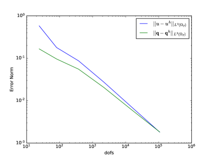
(a) Linear polynomial approximations.

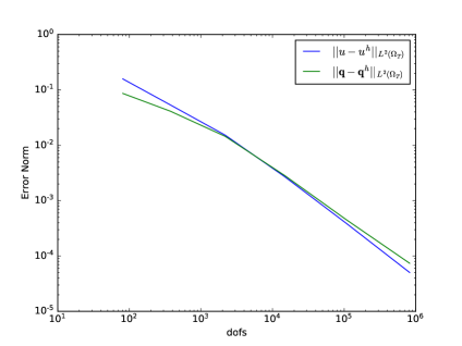
(b) Quadratic polynomial approximations.

Figure 2: Convergence histories for the space-time convergence study.

In Figure 2, we plot error norms versus the number of degrees of freedom $N$, which increases at $\mathcal{O}(h^{-2})$, i.e., the $h-$convergence rates of the FE approximations can be extracted from these by a simple adjustment. For the case of $\|{u-u^{h}}\|_{L^{2}(\Omega_{T})}$, we get $\mathcal{O}(N^{-1})=\mathcal{O}(h^{2})=\mathcal{O}(h^{p+1})$ order of convergence. The observed rates for $\|{\mathbf{q}-\mathbf{q}^{h}}\|_{L^{2}(\Omega_{T})}$ are slightly lower, whereas the energy error converges at the expected rates of $\mathcal{O}(h^{p})$. In error bounds for the AVS-FE method applied to a second order PDE, see, e.g, [42], it is only guaranteed that the energy norm (9) and the error in the norm on $U(\Omega_{T})$ converges at $\mathcal{O}(h^{p})$.

Analogously, in Figure 3, the convergence plots for generalized-$\alpha$ are presented for to study the convergence of the method at the final time $T=0.5s$ with time step of $\tau=10^{-3}$.

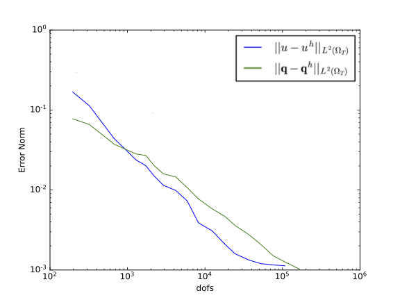
(a) Linear polynomial approximations, $\rho_{\infty}=0$.

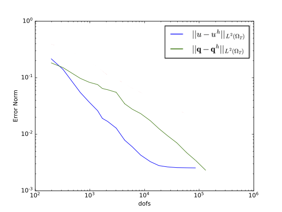
(b) Linear polynomial approximations, $\rho_{\infty}=0.9$.

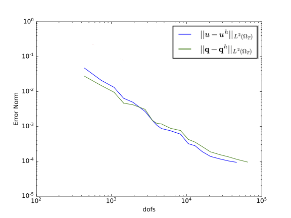
(c) Quadratic polynomial approximations, $\rho_{\infty}=0$.

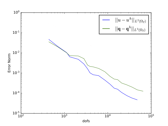
(d) Quadratic polynomial approximations, $\rho_{\infty}=0.9$.

Figure 3: Convergence study of the solution obtained using the generalized-$\alpha$ method for time discretization at final time $T=0.5\,s$.

The observed rates of convergence in Figure 3 are the optimal rates expected from the polynomial approximations employed. Note that the $L^{2}$ errors in the base variable $u$ becomes flat near the end of the refinement process as the temporal discretization error becomes dominant. Comparison of the results in Figures 2 and 3 for the two methods reveal that the number of degrees of freedom is significantly larger for the space-time approach.

4.2.1 $H-div$ Conforming Basis Functions

To complete our numerical verifications we consider the generalized-$\alpha$ system (32) and use Raviart-Thomas basis functions for the flux $q^{h}$. Following the know results from e.g., [33], the Raviart-Thomas functions are of order $p-1$, where $p$ is the order of the approximations for $u^{h}$. We also use discontinuous Raviart-Thomas bases for the vector valued error representation function of order $p$ and the scalar valued function of the same order $p$.

We again consider the same Eriksson-Johnson problem with $T_{final}=1.0s$, set $\epsilon=1\times 10^{-3}$, $p=2$, $\rho_{\infty}=0.9$ and perform both uniform and mesh refinements. In Figure 4, we present the corresponding convergence histories. Clearly, for the strongly convection-dominated case considered, the uniform refinements are not an optimal choice. However, the adaptive refinement scheme performs significantly better and is able to reduce the considered errors approximately two orders of magnitude.

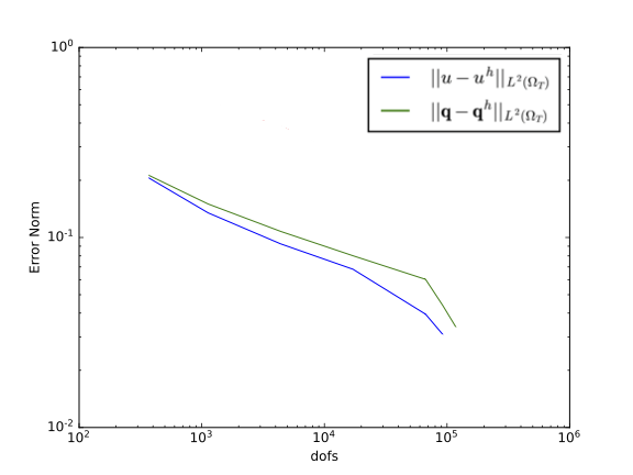
(a) Uniform mesh refinements.

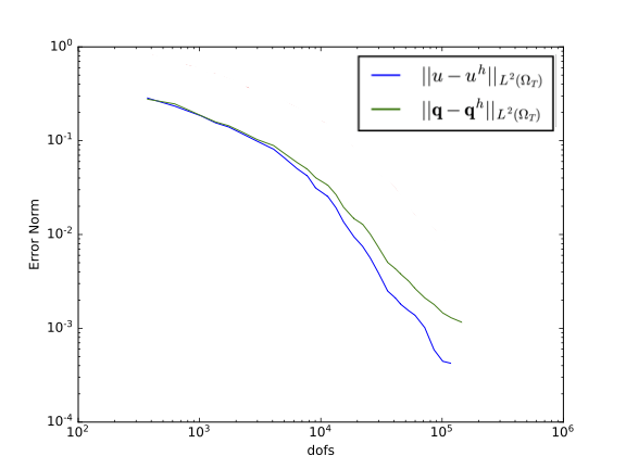
(b) Adaptive mesh refinements.

Figure 4: Convergence study of the solution obtained using the generalized-$\alpha$ approach $T=1.0$ using fully conforming FE basis functions.

4.2.2 Comparison Between Space-Time and Time Stepping

As the space-time and time-stepping methods are fundamentally different, a comparison between the two methods is not trivial. Comparison of accuracy of the two methods is not straightforward to compare, as the errors reported in Figure 2 are global for the full space-time domain and the errors in Figure 3 are at the final time step. Furthermore, the computational cost is distributed differently in the two methods. To provide a heuristic comparison between the two methods, we compare the error at the final time $T=0.5$ for the case of $p=1$ with the problem setup from Section 4.2. In the space-time approach the initial mesh consists of six uniform space-time tetrahedrons whereas in the GA method it consists of two triangular elements. In the GA method we set $\rho_{\infty}=0.9$ and perform 5 time steps. We perform uniform to the initial mesh and compute the errors in the space-time approach at the final time step and plot them alongside the final time error from generalized-$\alpha$ against the (2 dimensional) element size $h$ at the final time in Figure 5. It is interesting to observe that the errors in both methods shown in this figure are nearly identical. In terms of computational time, the space-time approach required 75 seconds whereas the GA method took 49 seconds. In both cases the experiments were performed on a 2022 MacBook pro with the Apple M2 chip.

Figure 5: Convergence at the final time $T=0.5$ for increasingly fine uniform meshes.

4.3 Shock Problem

As a final numerical verification, we present a consideration of (41) in which the solution behaves as two shocks traveling through the space-time domain while rotating about the origin. Furthermore, the choices we make for the problem parameters are such that the interface of the shock is skewed and rotates in the space-time domain as $t\rightarrow T_{final}$. Thus, we have the following choices:

$$\begin{array}[]{rl}\displaystyle\hfil&\{-x+2y,0\}^{T},\\ \displaystyle u_{0}=&0,\\ \displaystyle\epsilon=&10^{-3},\\ \displaystyle u_{0}=&0,\\ \displaystyle f=&-2x\epsilon+x(1-y^{2}).\\ \displaystyle T_{final}=&2.50s\\ \displaystyle\Omega=&(-1,1)\times(-1,1)\\ \end{array}$$ (46)

For this particular problem, we present the time slice approach in which we perform mesh adaptations between each slice and we apply linear polynomial approximations for the trial functions. Experience has shown that the slice containing the initial condition is critical to the proper resolution of the space-time process. Thus, we consider the case of three space-time slices, the first from $0s$ to $0.2s$ and the final two of equal size from $0.2s$ to $2.5s$. In Figures 6, 7, and 8 we present the AVS-FE solution for the base variable at different time steps. As expected, two shock-waves originate at the boundaries of $x=\pm 1$, and as time progress, the two waves approach the center of the domain while rotating. The adaptively refined meshes shown in Figures 6(b),  7(b), and 8(b) (the final times of each slice) show that the mesh refinements are focused at the interfaces of the shocks, further indicating the applicability of the built-in error indicators.

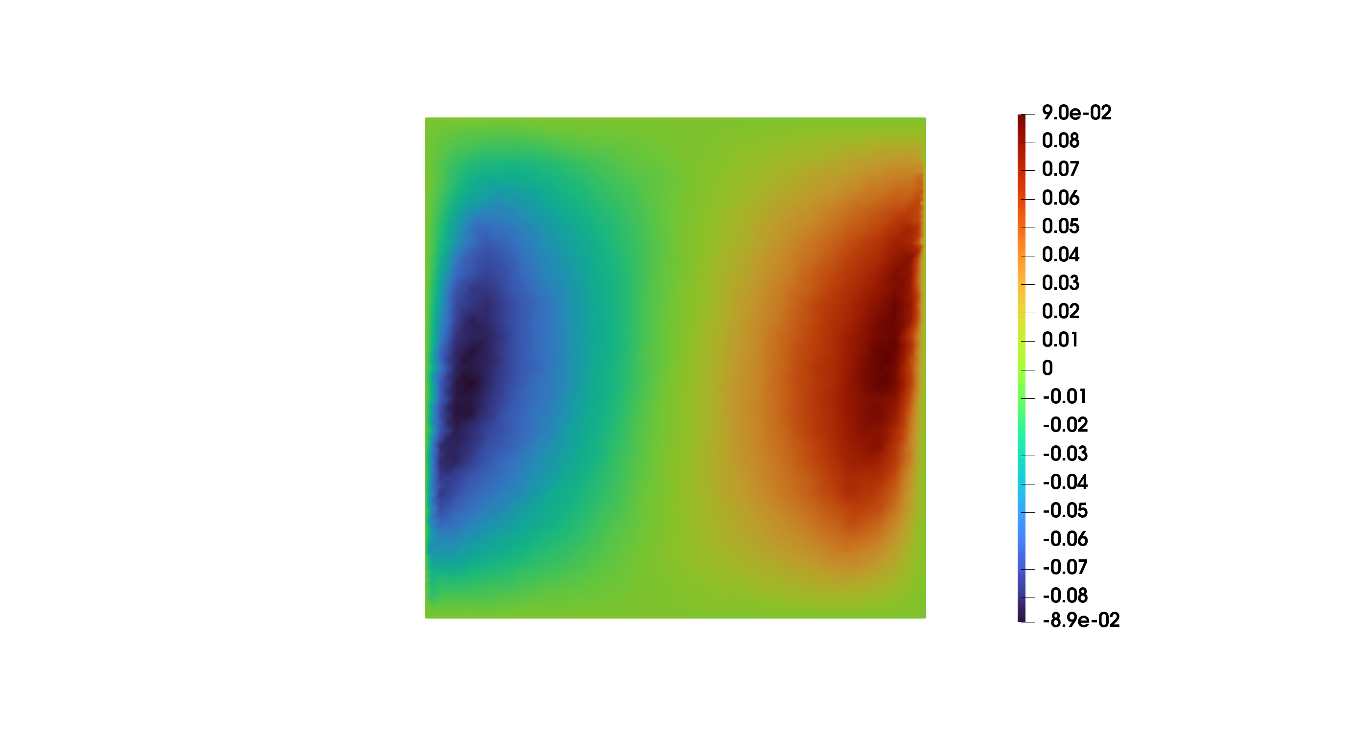
(a) Solution $u^{h}$ at $t=0.1s$.

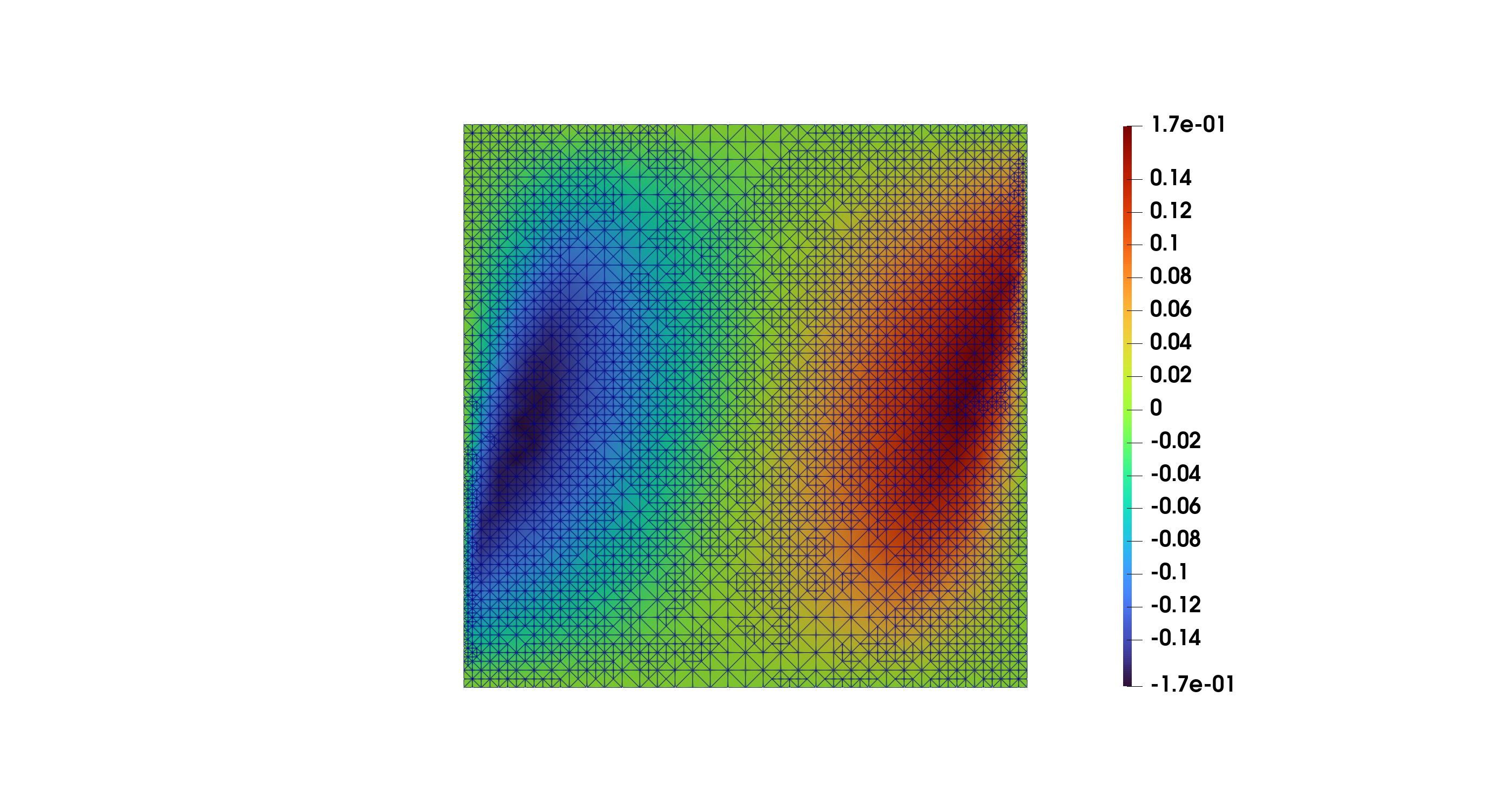
(b) Solution $u^{h}$ at $t=0.2s$ with final adapted mesh.

Figure 6: AVS-FE approximations of the shock problem, i.e., (41) with parameters from (46).

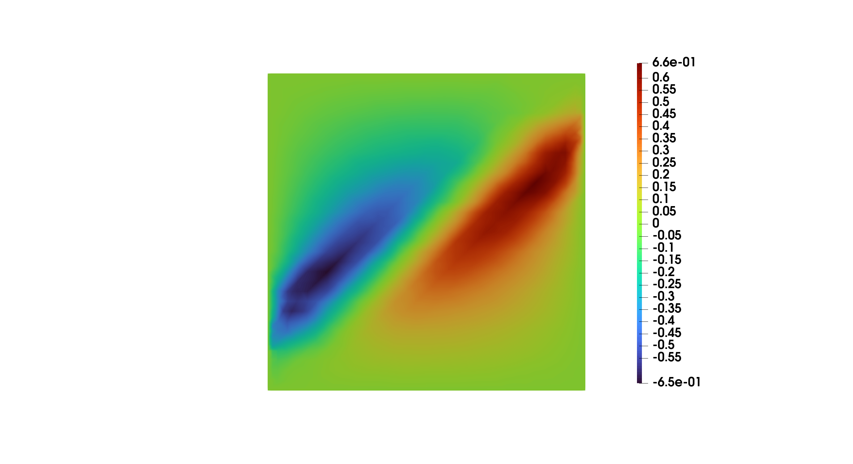
(a) Solution $u^{h}$ at $t=1.0s$.

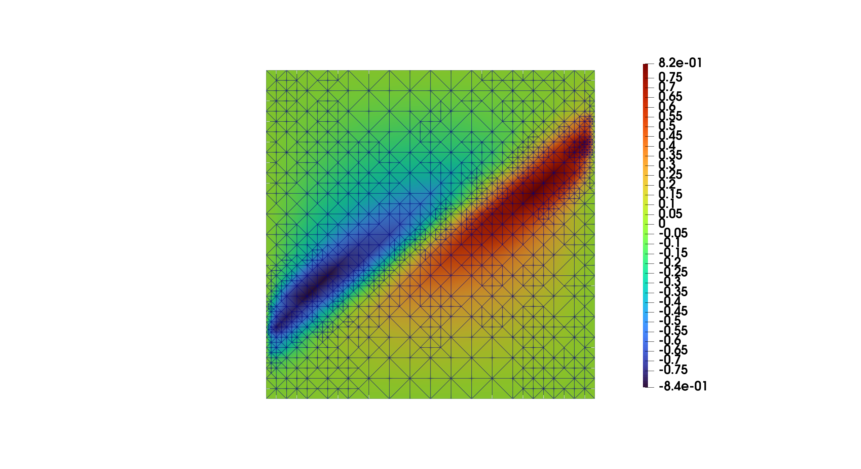
(b) Solution $u^{h}$ at $t=1.35s$ with final adapted mesh.

Figure 7: AVS-FE approximations of the shock problem, i.e., (41) with parameters from (46).

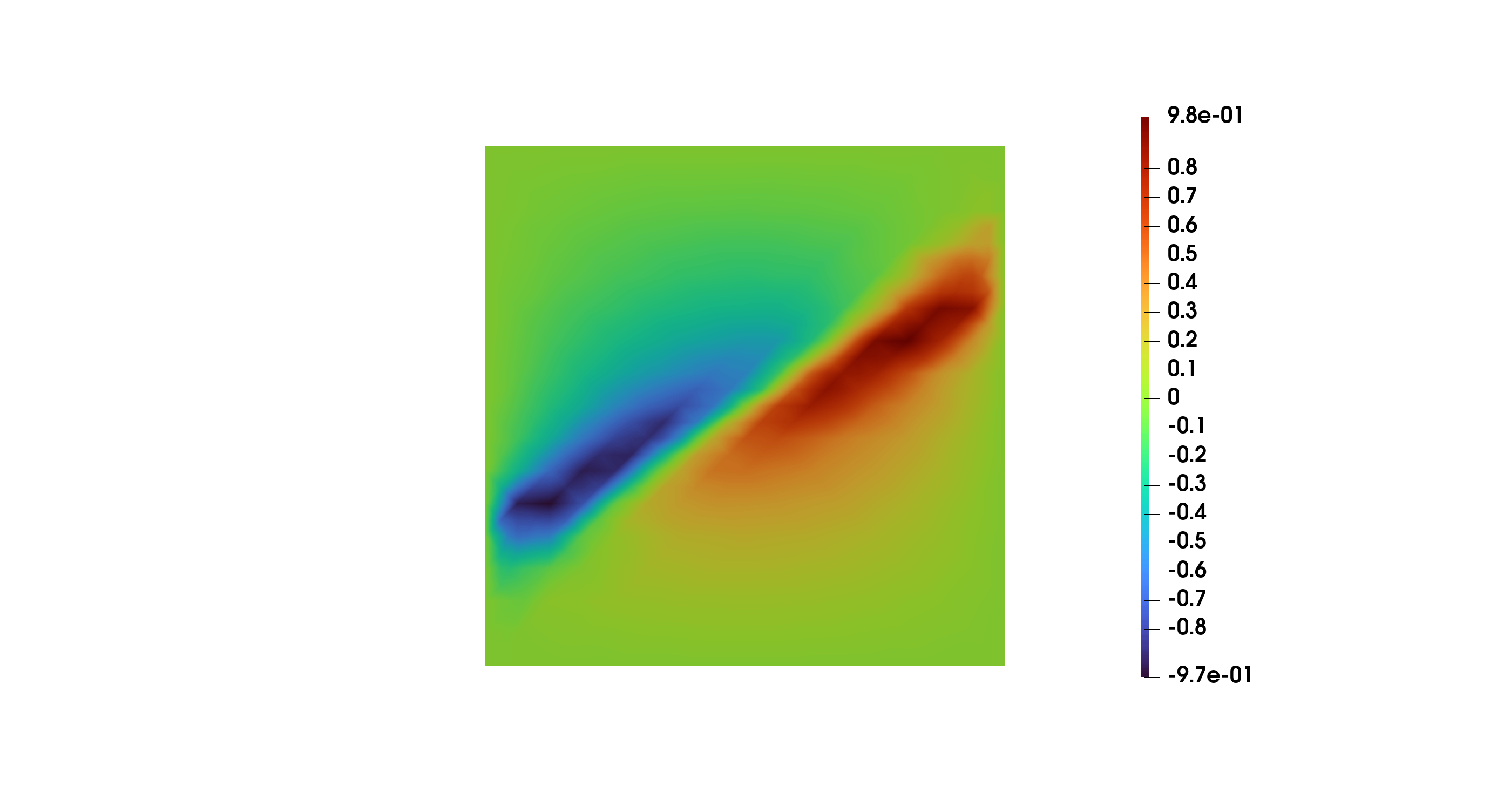
(a) Solution $u^{h}$ at $t=2.0s$.

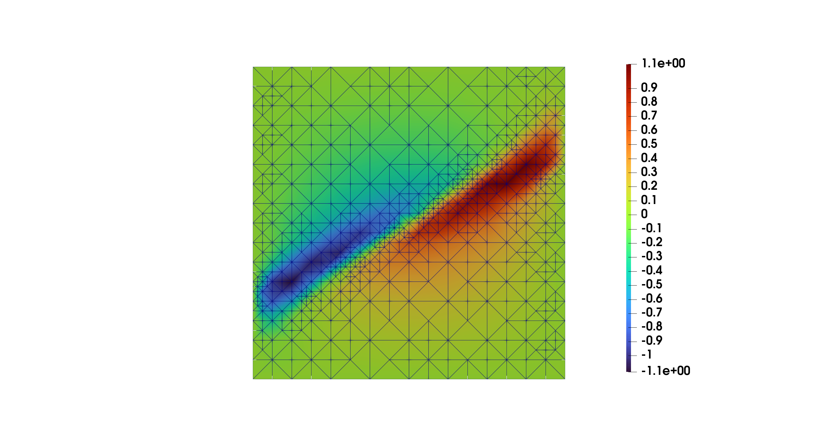
(b) Solution $u^{h}$ at $t=2.5s$ with final adapted mesh.

Figure 8: AVS-FE approximations of the shock problem, i.e., (41) with parameters from (46).

5 Conclusions

The AVS-FE method is a Petrov-Galerkin method which uses classical continuous FE trial basis functions, while the test space consist of functions that are discontinuous across element edges. This broken topology in the test space allows us to employ the DPG philosophy and introduce an equivalent saddle point problem which we implement using high level FE solvers. We have introduced two distinct approaches to transient problems using the AVS-FE method. First, we take a space-time approach in which the entire space-time domain in discretized using finite elements, and second, using the method of lines to discretize the spatial domain independently to deliver a semi-discretized system. Then, using a time-marching method, we obtain a fully discrete system.

The space-time method allows us to exploit the unconditional stability of the AVS-FE method and perform a single global solve governing the FE approximation. As the AVS-FE approximations computed from the saddle point system (30) come with built-in error indicators, we are capable of utilizing mesh adaptive strategies in space and time. In an effort to control the computational cost of the space-time approach in solving the global system of equations, we consider a time slice approach. Here, the space-time domain is partitioned into finite sized space-time slices on which we employ the AVS-FE method. The advantage here is that the size of the global system is reduced and we are able to employ mesh adaptive strategies on each slice.

The method of lines, in which we use the AVS-FE method for the spatial discretization and a generalized-$\alpha$ method to derive a fully-discretized system. In this case, the discrete stability in the temporal domain is ensured by the generalized-$\alpha$ method leading to highly efficient stable FE computations. We show that the AVS-FE method uses a corresponding norm as a function of the time-step. Another distinguishing feature of this method is that due to the influence of the initial data on the accuracy of the solution, we find a stable approximation for $\frac{\partial u}{\partial t}$ at the initial time. Accordingly, at each time step, one requires to solve a system with a smaller number of degrees of freedom in comparison with the space-time approach.

Numerical verifications for several cases of the transient convection-diffusion IBVP show that both methods exhibit optimal asymptotic convergence behavior as well as similar norms of the numerical approximation error. For degrees of approximation above $2$, the space-time approach becomes more accurate as it is not limited to the second-order accuracy of the generalized-$\alpha$ method. However, we do not advocate one method over the other but we point out these differences for potential users as their available computational resources will likely dictate which approach to use. For both cases, we present additional numerical verifiactions highlighting the adaptive mesh refinement capabilities. In future efforts, we expect to pursue alternative error estimators and indicators as well as the AVS-FE approximation of challenging transient physical phenomena. The use of basis functions that are of higher order regularity, e.g, as in [43] is another potential direction of future research efforts.

References

- [1] V. M. Calo, A. Romkes, E. Valseth, Automatic variationally stable analysis for FE computations: an introduction, in: Barrenechea G., Mackenzie J. (eds) Boundary and Interior Layers, Computational and Asymptotic Methods BAIL 2018, Springer, 2020, pp. 19–43.
- [2] L. Demkowicz, J. Gopalakrishnan, A class of discontinuous Petrov-Galerkin methods. Part I: The transport equation, Computer Methods in Applied Mechanics and Engineering 199 (23) (2010) 1558–1572.
- [3] C. Carstensen, L. Demkowicz, J. Gopalakrishnan, A posteriori error control for DPG methods, SIAM Journal on Numerical Analysis 52 (3) (2014) 1335–1353.
- [4] L. Demkowicz, J. Gopalakrishnan, Analysis of the DPG method for the Poisson equation, SIAM Journal on Numerical Analysis 49 (5) (2011) 1788–1809.
- [5] L. Demkowicz, J. Gopalakrishnan, A class of discontinuous Petrov-Galerkin methods. II. Optimal test functions, Numerical Methods for Partial Differential Equations 27 (1) (2011) 70–105.
- [6] L. Demkowicz, J. Gopalakrishnan, A class of discontinuous Petrov-Galerkin methods. Part III: Adaptivity, Applied numerical mathematics 62 (4) (2012) 396–427.
- [7] P. Behnoudfar, Q. Deng, V. M. Calo, High-order generalized-alpha method, Applications in Engineering Science 4 (2020) 100021.
- [8] P. Behnoudfar, Q. Deng, V. M. Calo, Higher-order generalized- methods for hyperbolic problems, Computer Methods in Applied Mechanics and Engineering 378 (2021) 113725.
- [9] J. Chung, G. Hulbert, A time integration algorithm for structural dynamics with improved numerical dissipation: the generalized- method, Journal of Applied Mechanics 60 (2) (1993) 371–375.
- [10] T. J. R. Hughes, J. R. Stewart, A space-time formulation for multiscale phenomena, Journal of Computational and Applied Mathematics 74 (1996) 217–229.
- [11] T. J. Hughes, G. M. Hulbert, Space-time finite element methods for elastodynamics: formulations and error estimates, Computer methods in applied mechanics and engineering 66 (3) (1988) 339–363.
- [12] A. K. Aziz, P. Monk, Continuous finite elements in space and time for the heat equation, Mathematics of Computation 52 (186) (1989) 255–274.
- [13] E. Valseth, A. Romkes, A. R. Kaul, A stable FE method for the space-time solution of the Cahn-Hilliard equation, Journal of Computational Physics 441 (2021) 110426.
- [14] E. Valseth, C. Dawson, An unconditionally stable space–time FE method for the Korteweg–de Vries equation, Computer Methods in Applied Mechanics and Engineering 371 (2020) 113297. doi:https://doi.org/10.1016/j.cma.2020.113297.
- [15] T. E. Ellis, L. Demkowicz, J. Chan, R. D. Moser, Space-time DPG: Designing a method for massively parallel CFD, ICES report, The Institute for Computational Engineering and Sciences, The University of Texas at Austin (2014) 14–32.
- [16] T. Ellis, J. Chan, L. Demkowicz, Robust DPG methods for transient convection-diffusion, in: Building bridges: connections and challenges in modern approaches to numerical partial differential equations, Springer, 2016, pp. 179–203.
- [17] N. V. Roberts, L. Demkowicz, R. Moser, A discontinuous Petrov–Galerkin methodology for adaptive solutions to the incompressible Navier–Stokes equations, Journal of Computational Physics 301 (2015) 456–483.
- [18] N. V. Roberts, Camellia: A software framework for discontinuous Petrov–Galerkin methods, Computers & Mathematics with Applications 68 (11) (2014) 1581–1604.
- [19] J. Muñoz-Matute, D. Pardo, L. Demkowicz, A DPG-based time-marching scheme for linear hyperbolic problems, Computer Methods in Applied Mechanics and Engineering 373 (2021) 113539.
- [20] J. Muñoz-Matute, L. Demkowicz, D. Pardo, Error representation of the time-marching DPG scheme, Computer methods in applied mechanics and engineering 391 (2022) 114480.
- [21] K. E. Jansen, C. H. Whiting, G. M. Hulbert, A generalized- method for integrating the filtered Navier–Stokes equations with a stabilized finite element method, Computer Methods in Applied Mechanics and Engineering 190 (3-4) (2000) 305–319.
- [22] H. M. Hilber, T. J. Hughes, R. L. Taylor, Improved numerical dissipation for time integration algorithms in structural dynamics, Earthquake Engineering & Structural Dynamics 5 (3) (1977) 283–292.
- [23] W. Wood, M. Bossak, O. Zienkiewicz, An alpha modification of Newmark’s method, International Journal for Numerical Methods in Engineering 15 (10) (1980) 1562–1566.
- [24] P. B. Bochev, M. D. Gunzburger, Least-Squares Finite Element Methods, Vol. 166, Springer Science & Business Media, 2009.
- [25] V. M. Calo, A. Ern, I. Muga, S. Rojas, An adaptive stabilized conforming finite element method via residual minimization on dual discontinuous Galerkin norms, Computer Methods in Applied Mechanics and Engineering 363 (2020) 112891.
- [26] A. H. Niemi, N. O. Collier, V. M. Calo, Automatically stable discontinuous Petrov–Galerkin methods for stationary transport problems: Quasi-optimal test space norm, Computers & Mathematics with Applications 66 (10) (2013) 2096–2113.
- [27] S. Nagaraj, S. Petrides, L. F. Demkowicz, Construction of DPG Fortin operators for second order problems, Computers & Mathematics with Applications 74 (8) (2017) 1964–1980.
- [28] L. Demkowicz, P. Zanotti, Construction of DPG Fortin operators revisited, Computers & Mathematics with Applications 80 (11) (2020) 2261–2271.
- [29] M. S. Alnæs, J. Blechta, J. Hake, A. Johansson, B. Kehlet, A. Logg, C. Richardson, J. Ring, M. E. Rognes, G. N. Wells, The FEniCS project version 1.5, Archive of Numerical Software 3 (100) (2015) 9–23.
- [30] F. Rathgeber, D. A. Ham, L. Mitchell, M. Lange, F. Luporini, A. T. McRae, G.-T. Bercea, G. R. Markall, P. H. Kelly, Firedrake: automating the finite element method by composing abstractions, ACM Transactions on Mathematical Software (TOMS) 43 (3) (2017) 24.
- [31] L. F. Demkowicz, J. Gopalakrishnan, An overview of the discontinuous Petrov-Galerkin method, in: Recent developments in discontinuous Galerkin finite element methods for partial differential equations, Springer, 2014, pp. 149–180.
- [32] F. Fuentes, B. Keith, L. Demkowicz, P. Le Tallec, Coupled variational formulations of linear elasticity and the DPG methodology, Journal of Computational Physics 348 (2017) 715–731.
- [33] F. Brezzi, M. Fortin, Mixed and Hybrid Finite Element Methods, Vol. 15, Springer-Verlag, 1991.
- [34] F. Brezzi, On the existence, uniqueness and approximation of saddle-point problems arising from Lagrangian multipliers, Publications mathématiques et informatique de Rennes (S4) (1974) 1–26.
- [35] P. Behnoudfar, V. M. Calo, Q. Deng, P. D. Minev, A variationally separable splitting for the generalized- method for parabolic equations, arXiv preprint arXiv:1811.09351 (2018).
- [36] D. A. Di Pietro, A. Ern, Mathematical aspects of discontinuous Galerkin methods, Vol. 69, Springer Science & Business Media, 2011.
- [37] T. E. Ellis, Space-time discontinuous Petrov-Galerkin finite elements for transient fluid mechanics, Ph.D. thesis (2016).
- [38] W. Dörfler, A convergent adaptive algorithm for Poisson’s equation, SIAM Journal on Numerical Analysis 33 (3) (1996) 1106–1124.
- [39] P. R. Amestoy, A. Guermouche, J.-Y. L’Excellent, S. Pralet, Hybrid scheduling for the parallel solution of linear systems, Parallel computing 32 (2) (2006) 136–156.
- [40] P. R. Amestoy, I. S. Duff, J.-Y. L’Excellent, J. Koster, A fully asynchronous multifrontal solver using distributed dynamic scheduling, SIAM Journal on Matrix Analysis and Applications 23 (1) (2001) 15–41.
- [41] K. Eriksson, C. Johnson, Adaptive streamline diffusion finite element methods for stationary convection-diffusion problems, mathematics of computation 60 (201) (1993) 167–188.
- [42] E. Valseth, A. Romkes, A. R. Kaul, C. Dawson, A stable mixed finite element method for nearly incompressible linear elastostatics, International Journal for Numerical Methods in Engineering 122 (17) (2021) 4709–4729.
- [43] M. Łoś, J. Munoz-Matute, I. Muga, M. Paszyński, Isogeometric residual minimization method (iGRM) with direction splitting for non-stationary advection–diffusion problems, Computers & Mathematics with Applications 79 (2) (2020) 213–229.