Three-dimensional super-Yang–Mills theory on the lattice and dual black branes

Abstract

In the large-$N$ and strong-coupling limit, maximally supersymmetric SU($N$) Yang–Mills theory in $(2+1)$ dimensions is conjectured to be dual to the decoupling limit of a stack of $N$ D$2$-branes, which may be described by IIA supergravity. We study this conjecture in the Euclidean setting using nonperturbative lattice gauge theory calculations. Our supersymmetric lattice construction naturally puts the theory on a skewed Euclidean 3-torus. Taking one cycle to have anti-periodic fermion boundary conditions, the large-torus limit is described by certain Euclidean black holes. We compute the bosonic action—the variation of the partition function—and compare our numerical results to the supergravity prediction as the size of the torus is changed, keeping its shape fixed. Our lattice calculations primarily utilize $N=8$ with extrapolations to the continuum limit, and our results are consistent with the expected gravity behavior in the appropriate large-torus limit.

I Introduction

It has been conjectured Maldacena (1999); Itzhaki et al. (1998); Witten (1998); Aharony et al. (2000) that the large-$N$ limits of maximally supersymmetric Yang–Mills (SYM) theories, obtained from the dimensional reduction of $\mathcal{N}=1$ SYM in ten dimensions down to $(p+1)$ dimensions, are dual to string theories containing D$p$-branes. In the large-$N$ and strong-coupling limit this relates properties of gauge theories to the dual properties of D$p$-brane solutions in supergravity. The $p=3$ case is the AdS/CFT correspondence, which has received much attention, in part due to its additional conformal symmetries. For direct numerical tests of holographic duality the $p<3$ cases are more attractive to consider, as they feature more tractable gauge theories Schaich (2019).

For example, the D$0$-brane or $p=0$ case is a quantum-mechanical description well-known as the Banks–Fischler–Shenker–Susskind (BFSS) model de Wit et al. (1988); Banks et al. (1997). One of the earliest efforts to understand holographic duality in the quantum-mechanical case directly from non-perturbative gauge theory was described in Refs. Kabat and Lifschytz (2000); Kabat et al. (2001a, b). In recent years, good agreement has been obtained for the case of $p=0$ in the Euclidean setting using numerical Monte Carlo calculations. These efforts started with Refs. Hanada et al. (2007); Catterall and Wiseman (2007); Anagnostopoulos et al. (2008); Catterall and Wiseman (2008); Hanada et al. (2009); Catterall and Wiseman (2010), and more sophisticated recent lattice analyses give convincing agreement with dual-gravity black hole predictions in the large-$N$ low-temperature limit Kadoh and Kamata (2015); Filev and O’Connor (2016); Berkowitz et al. (2016a, b). In addition to the BFSS quantum mechanics, a maximally supersymmetric deformation of it known as the Berenstein–Maldacena–Nastase (BMN) model Berenstein et al. (2002) which may also be dual to black holes at low temperatures Costa et al. (2015), is now also starting to be studied on the lattice Catterall and van Anders (2010); Asano et al. (2018); Schaich et al. (2020a).

This Euclidean lattice approach was extended to the higher-dimensional D$1$-brane case in Refs. Catterall et al. (2010); Kadoh (2017); Catterall et al. (2018a); Jha et al. (2018). To allow numerical lattice calculations, one must compactify the spatial direction. In the continuum this corresponds to placing the dual theory on a Euclidean torus with all bosonic fields subject to periodic boundary conditions along all directions. With periodic fermion boundary conditions along all directions, supersymmetry is unbroken and the partition function is independent of the size and shape of this torus. In order to study more interesting behavior, we take one cycle to be anti-periodic for fermions.

As discussed in Refs. Catterall et al. (2018a); Jha et al. (2018), a conventional thermodynamic interpretation would require the gauge theory to be on a rectangular torus with anti-periodic fermion (thermal) boundary conditions on the Euclidean time cycle. However, often it is more convenient to work with a skewed torus in the Euclidean setting, in order to use supersymmetric lattice actions which employ non-cubical lattices with enhanced point group symmetries. While one cannot continue the numerical results to Lorentzian signature due to the skewing, this is not an obstruction to testing supergravity predictions. One may also consider the dual supergravity in the Euclidean setting with a skewed torus as the asymptotic boundary geometry, in which case in the appropriate large-$N$ ’t Hooft limit it predicts a behavior governed by certain Euclidean black holes (which also have no Lorentzian analog).

The higher-dimensional SYM theories, such as the one considered in this paper, involve more challenging calculations than in the quantum-mechanical case, but offer the advantage of richer structures. Distinct phases are associated to center symmetry breaking signaled by the eigenvalue distributions of the Wilson lines around the spatial torus cycles, and are described in the dual gravity by the competition between different black hole solutions. In Refs. Catterall et al. (2018a); Jha et al. (2018) these different phases were indeed seen in two-dimensional lattice calculations, and reasonable agreement was observed for the variation of the partition function with torus size for both IIA and IIB supergravity predictions. (See Ref. Hiller et al. (2005) for an alternate approach to the strong-coupling limit of the $p=1$ theory in the Lorentzian signature.)

The purpose of this paper is to advance these tests of holographic duality to the next higher dimension — the case of D$2$-branes. Again we consider the Euclidean theory compactified on a torus so that it is amenable to lattice calculations. We take one anti-periodic cycle for fermions. In the conventional Euclidean thermal setting on a rectangular torus, the system has an even richer phase structure than the case of $p=1$, with sensitivity to the dimensionless temperature and the various aspect ratios of the 3-torus Susskind (1997); Martinec and Sahakian (1999). We consider here the skewed torus, as dictated by our supersymmetric lattice discretization. Keeping the shape of the torus fixed, we vary its size relative to the scale set by the ’t Hooft coupling and study the bosonic action—the variation of the partition function. We choose the shape of the torus so that we can expect the behavior in the large-$N$ strongly coupled large-torus limit to be governed by the simplest gravitational dual, a homogeneous Euclidean D$2$-brane black hole in IIA supergravity with boundary given by the skewed torus. We then numerically analyze this large-$N$, large-torus limit, to understand how well the gauge theory matches the predictions of the supergravity solution.

We begin in the next section by discussing $(2+1)$-dimensional SYM on a skewed torus and its supergravity dual in the large-$N$ ’t Hooft limit. In Section III we describe our three-dimensional supersymmetric lattice construction, which produces the numerical results presented and compared with supergravity expectations in Section IV. The data leading to these results are available at Catterall et al. (2020). We conclude in Section V by looking ahead to further lattice SYM studies that can build on this work in the future, including prospects for exploring phase transitions by changing the shape of the torus.

II SYM on a skewed torus and the supergravity dual

We consider three-dimensional maximally supersymmetric Yang–Mills theory, which we take in Euclidean signature to be on a 3-torus denoted hereafter by $\mathbb{T}^{3}$. As in the thermal case, we impose anti-periodic fermion boundary conditions only on one cycle corresponding to Euclidean time. Labelling this coordinate as $\tau$, and the others as $x_{i}$, we identify $\tau\sim\tau+\beta$ (anti-periodic for fermions), while the others form the ‘spatial’ torus cycles after the identifications $(\tau,x_{i})\sim(\tau,x_{i})+\vec{L}_{1,2}$ (periodic for fermions). If $\vec{L}_{1,2}$ were orthogonal to each other and $\tau$, the torus would be rectangular and we would have a Lorentzian interpretation with $\beta$ being the inverse temperature. Here we will consider a skewed torus, for which there is no simple Lorentzian interpretation — the Euclidean torus cannot be analytically continued to a real Lorentzian-signature space-time. Nonetheless, holographic duality states that this theory can be described by a string theory dual which reduces to supergravity in the large-$N$ ’t Hooft limit.

It is convenient to define dimensionless lengths $r_{\tau}=\beta\lambda$ and $r_{1,2}=|\vec{L}_{1,2}|\lambda$ in terms of the (dimensionful) ’t Hooft coupling $\lambda=Ng_{\text{YM}}^{2}$. Here we are interested in fixing the shape of the torus that the SYM is defined on, while varying its size. Thus we make the choice $\vec{L}_{1,2}=\beta\vec{l}_{1,2}$, with $\vec{l}_{1,2}$ being vectors that we take to be fixed with unit length, $|\vec{l}_{1,2}|=1$, so that each torus cycle has equal proper length $\beta$. The partition function of the Euclidean theory is then just a function of the one dimensionless parameter $r_{\tau}$, and it is convenient to think in terms of $t=1/r_{\tau}$, which we may view as a dimensionless ‘generalized’ temperature. At large $N$ in the ’t Hooft limit we regard $t\sim O(1)$. In this limit, a large numerical value $t=1/r_{\tau}\gg 1$ corresponds to the torus being small in units of the ’t Hooft coupling, and the theory reduces to a 0-dimensional effective theory of the zero modes on the torus. This small-torus effective theory corresponds to the bosonic Yang–Mills matrix integral formed from the bosonic truncation of the $p=0$ SYM theory, which we note is not a weakly coupled description Aharony et al. (2004, 2006).

Conversely, a small numerical value $t=1/r_{\tau}\ll 1$ corresponds to the torus being large in units of the ’t Hooft coupling. The behavior in this regime is given by the decoupling limit of D$2$-branes Itzhaki et al. (1998), which may be described in supergravity by the ten-dimensional Euclidean string frame metric and dilaton,

$$\begin{split}ds^{2}_{\text{IIA, String}}&=\alpha^{\prime}\left(\frac{U^{5/2}}{\sqrt{6\pi^{2}\lambda}}\left[\left(1-\frac{U_{0}^{5}}{U^{5}}\right)d\tau^{2}+dx_{i}^{2}\right]+\frac{\sqrt{6\pi^{2}\lambda}}{U^{5/2}}\left[dU^{2}\left(1-\frac{U_{0}^{5}}{U^{5}}\right)^{-1}+U^{2}d\Omega^{2}_{(6)}\right]\right)\\ e^{\phi}&=\frac{\lambda}{N}\sqrt{\frac{6\pi^{2}\lambda}{U^{5/2}}}.\end{split}$$ (1)

There is also a 3-form potential carrying the $N$ units of D$2$-charge, with $\tau$ and $x_{i}$ forming the ‘world-volume’ directions that constitute the asymptotic toroidal boundary which we may think of the gauge theory living on. Here $U$ is the radial direction, normalized as an energy scale, and $U_{0}$ represents the radial position of a Euclidean ‘horizon’ where the Euclidean time circle direction, $\tau$, shrinks to zero size. The smoothness of the geometry relates this to the inverse temperature $\beta$, as $U_{0}^{3/2}=\frac{4\pi^{2}}{5}\frac{\sqrt{6\lambda}}{\beta}$. We require large $N$ to suppress string quantum corrections to the supergravity approximation, while the large torus size, $t\ll 1$, is required to suppress the $\alpha^{\prime}$ corrections to the classical supergravity geometry near the horizon. Both these conditions are satisfied if we take $1\ll r_{\tau}\ll N^{\frac{6}{5}}$ at large $N$, which is the regime we focus on in this work.

On a large torus with $t\ll 1$, stringy winding modes along the $x_{i}$ cycles may become relevant, associated to a T-dual Gregory–Laflamme instability Gregory and Laflamme (1993); Susskind (1997); Barbon et al. (1999); Li et al. (1999); Martinec and Sahakian (1999); Aharony et al. (2004, 2006), in the case that $r_{1,2}^{3/2}\lesssim r_{\tau}$. However, since we are fixing the shape of the torus to have $r_{1,2}=r_{\tau}$, we do not expect such phenomena to occur in a regime where the dual supergravity describes the system. Since the dual D$2$-brane solution has non-contractible spatial cycles on the torus, we expect the angular distribution of eigenvalues of a Wilson line about such a cycle to be homogeneous at large $N$ Maldacena (1998); Witten (1998); Aharony et al. (2004). On the other hand, for a small torus where the theory reduces to a bosonic matrix integral, we expect a highly localized distribution of eigenvalue phases for Wilson lines about any torus cycle. Hence one expects a large-$N$ transition as the torus size is varied, associated to center symmetry breaking of the spatial Wilson lines.

If the $x_{i}$ directions were not compact, so that $T=1/\beta$ is a temperature, then noting that the solution is translation invariant in the $\tau$ and $x_{i}$ directions, one may compute the free energy density $f$ from the dual-gravity solution,

$$\frac{f}{N^{2}\lambda^{3}} =-\left(\frac{2^{13}3^{5}\pi^{8}}{5^{13}}\right)^{1/3}t^{10/3}\approx-2.49189\leavevmode\nobreak\ t^{10/3}\,.$$ (2)

Compactifying on a torus doesn’t change this density, and for a rectangular torus it yields a partition function $\log Z=-fV(\mathbb{T}^{3})$, where $V(\mathbb{T}^{3})$ denotes the volume of the 3-torus. Due to the translation invariance of the solution, the skewed-torus partition function is given by these same expressions, although there is no thermal interpretation Aharony et al. (2006).

The SYM action is composed of bosonic and fermionic parts having the schematic form

$$S_{\text{SYM}} =S_{\text{Bos}}+S_{\text{Ferm}}$$ (3)

$$S_{\text{Bos}} =\frac{N}{4\lambda}\int_{\mathbb{T}^{3}}d\tau d^{2}x\,\text{Tr}\left[F^{2}+2\left(D\Phi_{I}\right)^{2}-\left[\Phi_{I},\Phi_{J}\right]^{2}\right]$$ (4)

$$S_{\text{Ferm}} =\frac{N}{\lambda}\int_{\mathbb{T}^{3}}d\tau d^{2}x\,\text{Tr}\left[\psi^{T}\left(\not{D}-\left[\Gamma_{I}\Phi_{I},\cdot\right]\right)\psi\right].$$

Rescaling the gauge field $A$, scalars $\Phi_{I}$, fermions $\psi$, and the coordinates $(\tau,x_{i})$ by the torus size so they are all dimensionless,

$$(A,\Phi_{I}) =(A^{\prime},\Phi_{I}^{\prime})/\beta \psi =\sqrt{\lambda}\psi^{\prime}/\beta$$

$$(\tau,x_{i}) =\beta(\tau^{\prime},x_{i}^{\prime}),$$

the action may be written as

$$S_{\text{SYM}}=\frac{1}{\beta\lambda}S^{\prime}_{\text{Bos}}+S^{\prime}_{\text{Ferm}},$$ (5)

where $S^{\prime}_{\text{Bos}}=S_{\text{Bos}}\beta\lambda$ and $S^{\prime}_{\text{Ferm}}=S_{\text{Ferm}}$ involve only the dimensionless bosonic fields and fermion fields respectively, and have no explicit $\beta$ or $\lambda$ dependence. Thus we may explicitly differentiate the partition function with respect to $\beta$ to obtain

$$\beta\frac{\partial}{\partial\beta}\log Z=\left\langle S_{\text{Bos}}\right\rangle.$$ (6)

While the partition function itself cannot be computed through the lattice methods we use, the expectation value of the bosonic action is very convenient to obtain (as reviewed in the Appendix). We find the prediction from supergravity that at large $N$,

$$\frac{\left\langle S_{\text{Bos}}\right\rangle}{N^{2}} =-\left(\frac{2^{13}3^{2}\pi^{8}t}{5^{13}}\right)^{1/3}\left(\frac{V(\mathbb{T}^{3})}{\beta^{3}}\right)$$ (7)

when $t$ is sufficiently small. In the small-volume limit $t\gg 1$ we may use the effective dimensional reduction to compute

$$\frac{\left\langle S_{\text{Bos}}\right\rangle}{N^{2}}=-2$$ (8)

at large $N$ Kawahara et al. (2007); Catterall et al. (2018a).

We will see in the next section that the most natural torus geometry for us to consider is formed by periodically identifying $\mathbb{R}^{3}$ in the three basis directions of an $A_{3}^{*}$ lattice. As discussed above, we do so taking the cycle in each direction to have the same length $\beta$. Explicitly in our coordinates $x_{\mu}=(\tau,x_{i})$ we may achieve this by taking

$$\vec{l}_{1} =\frac{1}{3}\left(\begin{array}[]{c}-1\\ 2\sqrt{2}\\ 0\end{array}\right) \vec{l}_{2} =\frac{1}{3}\left(\begin{array}[]{c}-1\\ -\sqrt{2}\\ \sqrt{6}\end{array}\right),$$ (15)

which gives a volume $V(\mathbb{T}^{3})=4\beta^{3}/(3\sqrt{3})$.

Defining the bosonic action density $s_{\text{Bos}}=\left\langle S_{\text{Bos}}\right\rangle/V(\mathbb{T}^{3})$, for our torus geometry we see the holographic large-volume behavior and small-volume limit imply

$$\frac{s_{\text{Bos}}}{N^{2}\lambda^{3}}=\left\{\begin{array}[]{ll}-0.831\dots t^{10/3}&\mbox{for }t\ll 1\\ -2.598\dots t^{3}&\mbox{for }t\gg 1\end{array}\right..$$ (16)

It is worth noting that for SYM on an analogous torus in $(p+1)$-dimensions we would have parametric dependence $s_{\text{Bos}}\propto t^{(14-2p)/(5-p)}$ for $t\ll 1$ from the gravity dual, and the $t\gg 1$ limit would go as $s_{\text{Bos}}\propto t^{p+1}$. In the $p=3$ conformal case these powers coincide, and we see the powers in the case of $p=2$ we consider here are rather close. This makes the task of distinguishing the two behaviors more challenging than for the $p=0$ and $1$ cases considered previously Hanada et al. (2009); Catterall and Wiseman (2008); Berkowitz et al. (2016a, b); Kadoh (2017); Catterall et al. (2018a); Jha et al. (2018), where there is greater contrast between the large- vs. small-volume parametric dependence on $t$.

III Three-dimensional supersymmetric lattice construction

In recent years, it has become possible to formulate certain supersymmetric lattice gauge theories using the idea of topological twisting, in which the supercharges are grouped into $p$-forms and the $0$-form supercharges can be preserved in discrete space-time. While this construction is not needed for $(0+1)$-dimensional SYM quantum mechanics (where one can show perturbatively that no relevant supersymmetry-breaking counter-terms are possible Giedt et al. (2004); Catterall and Wiseman (2007)), in higher dimensions it is a key ingredient to minimize issues of fine-tuning Catterall et al. (2009); Schaich (2019).

The three-dimensional maximally supersymmetric Yang–Mills theory considered here can be obtained by classical dimensional reduction of four-dimensional $\mathcal{N}=4$ SYM. The $\mathcal{N}=4$ SYM lattice construction Kaplan and Ünsal (2005); Catterall (2008); Damgaard and Matsuura (2008); Catterall et al. (2012a, 2013, 2014a); Catterall and Giedt (2014); Schaich and DeGrand (2015); Catterall and Schaich (2015) discretizes a maximal twist of the continuum theory known as the Marcus or geometric-Langlands twist Marcus (1995); Kapustin and Witten (2007). The resulting lattice theory features many symmetries: in addition to U($N$) lattice gauge invariance and a single scalar supersymmetry, it is also invariant under a large $S_{5}$ point group symmetry arising from the underlying $A_{4}^{*}$ lattice. Using these symmetries, it is possible to show in perturbation theory that radiative corrections generate only a small number of log divergences in the lattice theory Catterall et al. (2013). On reduction to three dimensions these divergences disappear and no fine-tuning is expected to be needed to take the continuum limit Kaplan and Ünsal (2005). The resulting three-dimensional lattice theory naturally lives on an $A_{3}^{*}$ (body-centered cubic) lattice, whose four basis vectors correspond to vectors drawn out from the center of an equilateral tetrahedron to its vertices.

As we did in Refs. Catterall et al. (2018a); Jha et al. (2018), here we use the full four-dimensional lattice construction provided by the publicly available parallel software described in Refs. Schaich and DeGrand (2015); Schaich et al. (2020b), setting $N_{z}=1$ to reduce to the $A_{3}^{*}$ lattice. The remaining lattice directions are taken to have equal numbers of lattice sites, $N_{x}=N_{y}=N_{\tau}$, with anti-periodic fermion boundary conditions only on the $N_{\tau}$ cycle. In the continuum limit this generates the skewed torus geometry described in Section II (re-labelling $\{x_{1},x_{2}\}$ as $\{x,y\}$).

We relegate the full details of the lattice action $S_{\text{lattice}}$ to the Appendix, and here discuss only the two soft-supersymmetry-breaking deformation that need to be included in order to enable our three-dimensional numerical computations. The first of these is a scalar potential term, which regulates the divergences associated with integration over a non-compact moduli space in the partition function. We have used various scalar potentials in our previous investigations, and here employ the single-trace version also used in Refs. Catterall et al. (2018a); Jha et al. (2018):

$$S_{\text{soft}}=\frac{N}{4\lambda_{\text{lat}}}\mu^{2}\sum_{\mathbf{n},a}\text{Tr}\left[\bigg{(}\overline{\mathcal{U}}_{a}(\mathbf{n})\mathcal{U}_{a}(\mathbf{n})-\mathbb{I}_{N}\bigg{)}^{2}\right],$$ (17)

with $\mu^{2}$ a tunable coefficient and the dimensionless $\lambda_{\text{lat}}$ defined in the appendix. We need to extrapolate $\mu^{2}\to 0$ in order to recover the continuum SYM theory of interest, in addition to extrapolating to the continuum limit of vanishing lattice spacing that corresponds to $\lambda_{\text{lat}}\to 0$ in fewer than four dimensions. We guarantee that $\mu^{2}\to 0$ in the $\lambda_{\text{lat}}\to 0$ continuum limit by setting $\mu=\zeta\lambda_{\text{lat}}$. This also allows us to extrapolate $\mu^{2}\to 0$ with $\lambda_{\text{lat}}$ fixed by considering the $\zeta^{2}\to 0$ limit, which we will do in Section IV.

Next, for the dimensionally reduced lattice theory to correctly reproduce the continuum physics, we need to ensure that the trace of the each gauge link $\mathcal{U}_{z}(\mathbf{n})$ in the reduced $z$-direction is close to $N$, so that the effective scalar field obtained by dimensional reduction is small in lattice units. In other words, this means that the center symmetry should be completely broken in the reduced direction for proper dimensional reduction. We ensure this by adding a second soft-supersymmetry-breaking deformation to the lattice action:

$$S_{\text{center}}=\frac{N}{4\lambda_{\text{lat}}}\kappa^{2}\sum_{\mathbf{n}}\mbox{Tr}\bigg{[}\bigg{(}\mathcal{U}_{z}(\mathbf{n})-\mathbb{I}_{N}\bigg{)}^{{\dagger}}\bigg{(}\mathcal{U}_{z}(\mathbf{n})-\mathbb{I}_{N}\bigg{)}\bigg{]},$$ (18)

with $\kappa^{2}$ another tunable coefficient that we must also take to zero in Section IV. This term is gauge invariant since $N_{z}=1$. It explicitly breaks the center symmetry in the single reduced direction by forcing the trace of the link in this direction to be close to $N$.

With this lattice action $S_{\text{lattice}}$ for three-dimensional SYM, we stochastically sample field configurations using the rational hybrid Monte Carlo (RHMC) algorithm Clark and Kennedy (2007) implemented in the software mentioned above Schaich and DeGrand (2015); Schaich et al. (2020b). The RHMC algorithm treats $e^{-S_{\text{lattice}}}$ as a Boltzmann weight, requiring that we consider a lattice action that is real and non-negative. However, gaussian integration over the fermion fields of three-dimensional SYM produces a pfaffian that is potentially complex,

$$\int\left[d\Psi\right]e^{-\Psi^{T}\mathcal{D}\Psi}\propto\text{pf}\,\mathcal{D}=|\text{pf}\,\mathcal{D}|e^{i\phi}.$$ (19)

Here $\mathcal{D}$ is the fermion operator and $S_{\text{lattice}}=S_{\text{Bos}}+\Psi^{T}\mathcal{D}\Psi$, with $S_{\text{Bos}}$ the bosonic part of the lattice action.

As in our previous work Catterall et al. (2014a, b); Catterall and Schaich (2015); Schaich and Catterall (2017); Catterall et al. (2018a); Jha et al. (2018); Schaich (2019), we ‘quench’ the phase $e^{i\phi}\to 1$ to obtain a positive lattice action for use in the RHMC algorithm. Reweighting

$$\left\langle\mathcal{O}\right\rangle=\frac{\left\langle\mathcal{O}e^{i\phi}\right\rangle_{\text{pq}}}{\left\langle e^{i\phi}\right\rangle_{\text{pq}}}$$ (20)

is then required to recover expectation values from these phase-quenched (‘${}_{\text{pq}}$’) calculations, where

$$\left\langle\mathcal{O}\right\rangle_{\text{pq}} =\frac{\int[d\mathcal{U}]\ \mathcal{O}e^{-S_{\text{Bos}}}\ |\text{pf}\,\mathcal{D}|}{\int[d\mathcal{U}]\ e^{-S_{\text{Bos}}}\ |\text{pf}\,\mathcal{D}|}$$ (21)

$$\left\langle\mathcal{O}\right\rangle =\frac{\int[d\mathcal{U}]\ \mathcal{O}e^{-S_{\text{Bos}}}\ \text{pf}\,\mathcal{D}}{\int[d\mathcal{U}]\ e^{-S_{\text{Bos}}}\ \text{pf}\,\mathcal{D}}.$$ (22)

This procedure breaks down, producing a sign problem, when $\left\langle e^{i\phi}\right\rangle_{\text{pq}}$ is consistent with zero. Fortunately, in this investigation we focus on regimes where $\left\langle e^{i\phi}\right\rangle_{\text{pq}}\approx 1$ and $\left\langle\mathcal{O}\right\rangle\approx\left\langle\mathcal{O}\right\rangle_{\text{pq}}$. This follows from the fact that the $r_{\tau}$ and $N_{\tau}$ we analyze correspond to $0.14<\lambda_{\text{lat}}<1.34$, safely in the range of couplings where we observe $\left\langle e^{i\phi}\right\rangle_{\text{pq}}\approx 1$ in the full four-dimensional theory Catterall et al. (2014b); Schaich and Catterall (2017); Schaich (2019). In addition, we gain further benefit from the dimensional reduction, since the lower-dimensional continuum limit corresponds to $\lambda_{\text{lat}}\to 0$. Partly for this reason, previous lattice studies of $\mathcal{N}=(2,2)$ and $\mathcal{N}=(8,8)$ SYM theories in two dimensions found $\left\langle e^{i\phi}\right\rangle_{\text{pq}}\to 1$ rapidly upon approaching the continuum limit, with negligible pfaffian phase fluctuations even at non-zero lattice spacing Hanada and Kanamori (2011); Catterall et al. (2012b); Mehta et al. (2011); Galvez et al. (2011); Catterall et al. (2018b). Similarly small pfaffian phase fluctuations were also seen in the $p=0$ case Catterall and Wiseman (2010); Filev and O’Connor (2016).

IV Numerical results and comparison with supergravity

Figure 1: The $\zeta^{2}\to 0$ extrapolated bosonic action density for $N=8$ with lattice sizes $8^{3}$, $12^{3}$, and $16^{3}$, compared with the large-volume (dashed) and small-volume (solid) expectations from Eq. (16). Left: The full range of dimensionless temperatures $t$ on log–log axes. Right: Focusing on $0.2<t<0.48$ with linear axes to clarify the absolute size of uncertainties.

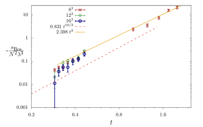
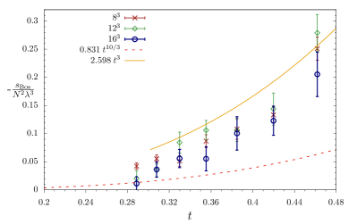
We now present our lattice results for the bosonic action density in the two different regimes described in Section II. Recall that the small-volume regime has dimensionless ‘generalized’ temperature $t\gg 1$, while $t\ll 1$ for the more interesting large-volume regime related to the dual supergravity by holography. We have concentrated resources to analyze these two regimes, with a focus on $0.25<t<0.5$. Our key result is Fig. 1 where we display the bosonic action density vs. $t$ for $N=8$ and the $L^{3}$ lattice sizes we consider, with $N_{x}=N_{y}=N_{\tau}=L=8$, $12$, and $16$.

After briefly discussing $t\geq 1$ results in the small-volume regime, which we use to check our lattice calculations, we focus on the more challenging large-volume case with $0.25<t<0.5$. This range of $t$ is chosen to satisfy the conditions $1\ll r_{\tau}\ll N^{\frac{6}{5}}$ discussed in Section II, which for $N=8$ correspond to $0.08\ll t\ll 1$. While it would be straightforward to run numerical calculations with smaller $t\lesssim 0.25$, for our current $N=8$ these may exit the regime in which IIA supergravity is a reliable description of the holographically dual gravitational system. Moving to larger $N>8$ is also possible, but would demand much more substantial computational resources due to computational costs increasing more rapidly than $N^{3}$ Schaich et al. (2020b). The results presented here required $\sim$$5$ million core-hours provided by multiple computing facilities, with costs dominated by the largest $L=16$ we consider. Ref. Catterall et al. (2020) provides a comprehensive release of our data, including full accounting of statistics, auto-correlation times, extremal eigenvalues of the fermion operator (which must remain within the spectral range where the rational approximation used in the RHMC algorithm is reliable), and other observables computed in addition to the bosonic action density.

IV.1 Small-volume regime, $t\gg 1$

To check that our lattice calculations reproduce the expected small-volume behavior of three-dimensional SYM, we analyze several large values of $t\geq 1$. Motivated by the right panel of Fig. 1, which shows no significant dependence on $L\geq 8$ for $t\gtrsim 0.3$, we carry out these calculations for a single $L^{3}$ lattice size with $L=8$. For these large $t$ we are also able to set $\kappa^{2}=0$ in Eq. (18) without encountering numerical instabilities (i.e., the center symmetry in the reduced direction breaks dynamically), leaving Eq. (17) the only soft-supersymmetry-breaking deformation in the lattice action. As discussed in Section III, we remove this deformation by extrapolating $\zeta^{2}\to 0$, here considering $\zeta^{2}=0.04$, $0.06$ and $0.09$ for each value of $t$. These linear extrapolations produce the $t\geq 1$ results in the left panel of Fig. 1, which are in good agreement with the solid line showing the expected small-volume limit from Eq. (16).

Figure 2: Distributions of $N=8$ Wilson line eigenvalue phases over the angular range $[-\pi,\pi)$, in the small-volume regime with dimensionless temperatures $t\geq 1$. The distributions become more localized with increasing $t$, as expected.

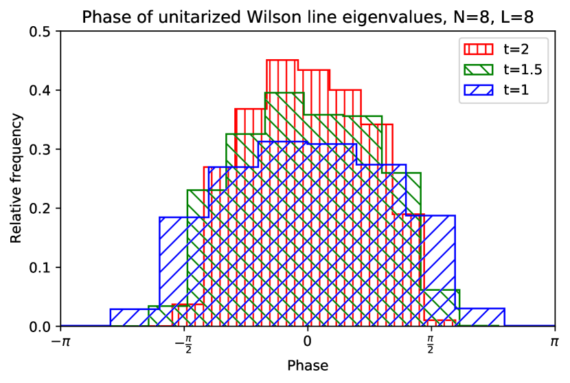
In Fig. 2 we show distributions of the phases of the Wilson line (spatial holonomy) eigenvalues for three $t\geq 1$ lattice ensembles with $\zeta^{2}=0.09$. As reviewed in the Appendix, our lattice construction naturally provides complexified Wilson lines that include contributions from both the gauge and scalar fields. In this work, we remove the scalar-field contributions by considering instead unitarized Wilson lines. The resulting distributions shown in Fig. 2 are clearly localized, and the width of the support decreases as $t$ increases. This lattice result is consistent with the expectation that the angular eigenvalue distribution is highly localized for $t\to\infty$, providing another non-trivial check that our lattice calculations correctly reproduce the three-dimensional SYM theory.

IV.2 Large-volume regime, $t\ll 1$

Turning now to the more interesting large-volume regime where we can compare our results with dual supergravity predictions, we analyze $0.25<t<0.5$ in order to satisfy the conditions $N^{-\frac{6}{5}}\ll t\ll 1$ discussed above, with $N^{-\frac{6}{5}}\approx 0.08$ for the $N=8$ we consider. In this regime, we need to include both soft-supersymmetry-breaking deformations Eqs. 17 and 18 in the lattice action. To simplify our analysis we set $\kappa^{2}=\mu^{2}$, so that each $\zeta^{2}\to 0$ extrapolation (here considering $\zeta^{2}=0.01$, $0.04$, and $0.09$) simultaneously removes both deformations. Control over these extrapolations is essential to precisely determine the SYM bosonic action density to be compared with the supergravity prediction.

Figure 3: Representative linear $\zeta^{2}\to 0$ extrapolations of the bosonic action density for different temperatures on $12^{3}$ lattices with $N=8$.

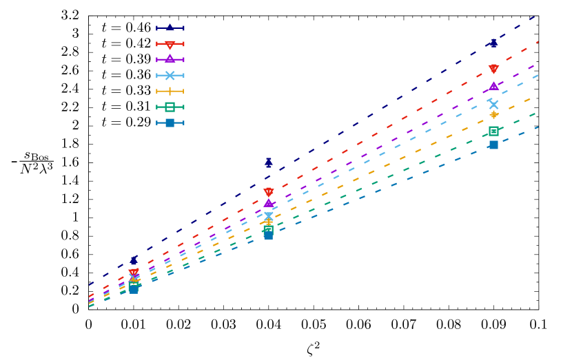
Representative linear $\zeta^{2}\to 0$ extrapolations of our bosonic action density data are shown in Fig. 3 for all our $12^{3}$ lattice ensembles with $N=8$. The $\zeta^{2}\to 0$ limits in this figure correspond exactly to the $12^{3}$ points shown in both panels of Fig. 1. Clearly the $\zeta^{2}\to 0$ extrapolated results in Fig. 1 have significantly larger relative uncertainties than the input data at non-zero $\zeta$ in Fig. 3. This is a consequence of the steep extrapolations to the much smaller SYM bosonic action densities that remain after removing the deformations in our lattice action.

Figure 4: Continuum extrapolations of the $\zeta^{2}\to 0$ extrapolated bosonic action density for various temperatures with $N=8$, where the limit $L^{2}\to\infty$ with fixed $t$ corresponds to $\lambda_{\text{lat}}\to 0$ and vanishing lattice spacing. Small horizontal offsets are added for clarity. All extrapolations for $t\geq 0.33$ have slopes consistent with zero, indicating no significant discretization artifacts in the corresponding results.

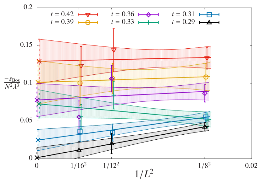
These larger uncertainties are even more evident in Fig. 4, where we zoom in on the six smallest $0.29\lesssim t\lesssim 0.42$ to investigate the dependence of the $\zeta^{2}\to 0$ extrapolated bosonic action densities on the $L^{3}$ lattice volume with $L=8$, $12$ and $16$. Since we fix the dimensionless lengths of the lattice, $r_{x}=r_{y}=r_{\tau}$, larger values of $L$ correspond to smaller lattice spacings, allowing us to check discretization artifacts and extrapolate to the continuum limit, $1/L^{2}\to 0$ or equivalently $L^{2}\to\infty$. Most of the linear $1/L^{2}\to 0$ extrapolations shown in Fig. 4 have slopes consistent with zero, indicating that there are not significant discretization artifacts in the corresponding results, and motivating our choice to include all our $L=8$, $12$ and $16$ results in Fig. 1. On the whole, these bosonic action density results are reasonably consistent with the large-$N$ prediction from supergravity in Eq. (16) (the dashed line in Fig. 1), particularly considering the modest $N=8$ and $t\approx 0.3$ that we have used in this work.

The best agreement with the dual supergravity prediction comes from the two smallest $t\approx 0.31$ and $0.29$, which are also the cases where the $1/L^{2}\to 0$ continuum extrapolations are non-trivial. From Fig. 4 we can see that these non-trivial extrapolations are driven by the $L=8$ results, with the $L=12$ and $16$ results fully consistent with the respective continuum limits within their (relatively large) uncertainties. An obvious question in this context is whether these results really fall in the large-volume regime, or may still be governed by small-volume (or intermediate) behavior. As discussed below Eq. (16), the expected parametric dependence of the bosonic action density is rather similar in both regimes for this $p=2$ case, making it more difficult to distinguish a clear change in behavior.

Figure 5: Distributions of Wilson line eigenvalue phases over the angular range $[-\pi,\pi)$ for a small $t\approx 0.31$. Left: The $L=12$ distributions become broader as $N$ increases, consistent with the homogeneous distribution expected for the large-volume regime in the large-$N$ limit. Right: The $N=8$ distributions are independent of the lattice size $L^{3}$.

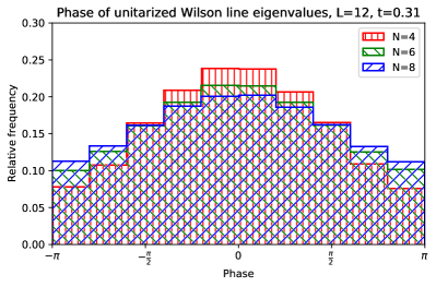
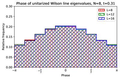
Stronger evidence that our small-$t$ results are in the large-volume regime can be obtained by again considering the eigenvalues of the Wilson line about the spatial torus cycles. In Fig. 5 we show distributions of the phases of these eigenvalues for lattice ensembles with $t\approx 0.31$ and $\zeta^{2}=0.09$, which follow broad distributions in clear contrast to the small-volume case shown in Fig. 2. Recall that the D$2$ supergravity solution predicts a homogeneous distribution of these phases at large $N$. To check the dependence on $N$, we have generated one $12^{3}$ ensemble with $N=4$ and another with $N=6$. In the left panel of Fig. 5 we compare the resulting $N=4$, $6$ and $8$ Wilson line eigenvalue phase distributions and confirm that they become broader as $N$ increases, consistent with the expected large-$N$ homogeneous distribution. In the right panel we check that there is no visible $L$ dependence in our $N=8$ results for this same $t\approx 0.31$ and $\zeta^{2}=0.09$. Thus we confirm that our small-$t$ results do indeed appear to be in the large-volume regime and consistent with the dual supergravity predictions. Presumably there is a large-$N$ phase transition separating the small- and large-volume regimes, although such a transition is difficult to see in our $N=8$ data on the lattice sizes we consider here.

V Conclusions and next steps

We have presented the first numerical lattice gauge theory studies of three-dimensional maximally supersymmetric Yang–Mills theory, advancing our program of non-perturbatively testing holography. Such tests provide direct first-principles checks of holographic duality at finite temperatures and in non-conformal settings, where tools such as integrability and supersymmetric localization are not available.

Already at modest $N=8$ our results indicate that the large-$N$ predictions of the dual-gravity black holes can emerge for large tori. We have seen that the bosonic action density interpolates rather smoothly between the small-volume regime and the large-volume supergravity regime, similar to results for lower-dimensional cases Hanada et al. (2009); Catterall and Wiseman (2008); Berkowitz et al. (2016a, b); Kadoh (2017); Catterall et al. (2018a); Jha et al. (2018). We are able to see qualitative agreement with the supergravity prediction derived from the dual black hole action density, and continuum extrapolations indicate no significant discretization artifacts for $t\geq 0.33$. We also see that the Wilson lines about the spatial directions of the torus are consistent with a transition from a localized angular eigenvalue distribution at small volumes to the expected homogeneous distribution at large volumes, presumably with a large-$N$ phase transition at an intermediate torus size.

In the future, we plan to look at the Maldacena–Wilson loop and compare it to the results obtained from the dual-gravity computations. In addition, similar to our previous study Catterall et al. (2018a); Jha et al. (2018), we can also change the aspect ratios of the torus cycle sizes to study phase transitions from the homogeneous D$2$-phase we consider here to D$1$-phases or even localized D$0$-phases. It will also be interesting to understand the nature of the large-$N$ phase transition at intermediate volumes, although this has proved difficult to study even in simpler settings Bergner et al. (2020).

Though our results approach the supergravity predictions in the appropriate regime, even larger $N$ would help to better satisfy the conditions on the validity of the classical supergravity description. Numerical calculations at larger $N$ are certainly possible, but would require much more substantial computational resources due to computational costs increasing more rapidly than $N^{3}$ Schaich et al. (2020b). Our current results in this paper nevertheless show the approach to this regime in detail and are certainly consistent with the supergravity results.

Appendix: Lattice action and computation of the bosonic action

Our lattice formulation of maximally supersymmetric Yang–Mills theory in $d<4$ dimensions discretized on the $A_{d}^{*}$ lattice is obtained by classical dimensional reduction from the parent four-dimensional theory. The lattice action for topologically twisted $\mathcal{N}=4$ SYM in $d=4$ dimensions is the sum of the following $\mathcal{Q}$-exact and $\mathcal{Q}$-closed terms Kaplan and Ünsal (2005); Catterall (2008); Damgaard and Matsuura (2008); Catterall et al. (2012a, 2013, 2014a); Catterall and Giedt (2014); Schaich and DeGrand (2015); Catterall and Schaich (2015):

$$S_{\text{exact}} =\frac{N}{4\lambda_{\text{lat}}}\sum_{\mathbf{n}}\text{Tr}\left[-\overline{\mathcal{F}}_{ab}(\mathbf{n})\mathcal{F}_{ab}(\mathbf{n})-\chi_{ab}(\mathbf{n})\mathcal{D}_{[a}^{(+)}\psi_{b]}^{\ }(\mathbf{n})-\eta(\mathbf{n})\overline{\mathcal{D}}_{a}^{(-)}\psi_{a}(\mathbf{n})+\frac{1}{2}\left(\overline{\mathcal{D}}_{a}^{(-)}\mathcal{U}_{a}(\mathbf{n})\right)^{2}\right],$$ (23)

$$S_{\text{closed}} =-\frac{N}{16\lambda_{\text{lat}}}\sum_{\mathbf{n}}\text{Tr}\left[{\epsilon_{abcde}\ \chi_{de}(\mathbf{n}+\widehat{\boldsymbol{\mu}}_{a}+\widehat{\boldsymbol{\mu}}_{b}+\widehat{\boldsymbol{\mu}}_{c})\overline{\mathcal{D}}_{c}^{(-)}\chi_{ab}(\mathbf{n})}\right],$$ (24)

where $\lambda_{\text{lat}}$ is the dimensionless ’t Hooft coupling defined by $r_{\tau,\text{lattice}}=\lambda_{\text{lat}}N_{\tau}^{4-d}$. The indices run from $1,\cdots,5$, spanning the basis vectors of the $A_{4}^{*}$ lattice, and $\sum_{\mathbf{n}}$ is over all lattice sites. The $1+5+10$ fermion fields $\eta$, $\psi_{a}$ and $\chi_{ab}=-\chi_{ba}$ transform in representations of the $S_{5}$ point group symmetry, as do the five complexified gauge links $\mathcal{U}_{a}$ and $\overline{\mathcal{U}}_{a}$ that combine the $4+6$ gauge and scalar field components. These gauge links are used to form the complexified field strengths $\mathcal{F}_{ab}$ and $\overline{\mathcal{F}}_{ab}$, as well as the finite difference operators $\mathcal{D}_{a}^{(+)}$ and $\overline{\mathcal{D}}_{a}^{(-)}$.

In addition to these terms, we also include the two soft-supersymmetry-breaking deformations discussed in Section III. $S_{\text{soft}}$ from Eq. (17) is present to regulate flat directions even in four dimensions, while $S_{\text{center}}$ from Eq. (18) needs to be added once we specialize to the three-dimensional theory by setting $N_{z}=1$. The full three-dimensional lattice action is then

$$S_{\text{lattice}} =S_{\text{exact}}+S_{\text{closed}}+S_{\text{soft}}+S_{\text{center}}.$$ (25)

As mentioned in Section IV.1, we can omit $S_{\text{center}}$ (by setting its coefficient $\kappa^{2}=0$) in the small-volume regime where the center symmetry in the reduced direction breaks dynamically.

Another detail mentioned in Section IV.1 is the need to remove the scalar-field contributions from the Wilson lines (spatial holonomies) that we analyze to distinguish between the small- and large-volume regimes. As in Ref. Catterall et al. (2014a, b, 2018a), we accomplish this by using a polar decomposition $\mathcal{U}_{a}=H_{a}\cdot U_{a}$ to separate each $N\!\times\!N$ complexified gauge link into a positive-semidefinite hermitian matrix $H_{a}$ (containing the scalar fields) and a unitary matrix $U_{a}$ corresponding to the gauge field. The resulting unitarized Wilson lines are simply the products $\prod_{i=1}^{N_{x}}U_{x}(x_{i},y,\tau)$ wrapping around the lattice, and similarly in the $y$-direction. The distributions shown in Figs. 2 and 5 come from the Wilson lines in the $x$-direction, while the data released in Ref. Catterall et al. (2020) confirm that Wilson lines in both spatial directions are equivalent, as they should be for the $N_{x}=N_{y}$ we consider.

Since the lattice basis vectors are not orthogonal, in $d<4$ dimensions the dimensionless lattice coupling $\lambda_{\text{lat}}$ has a non-trivial relation to the dimensionful continuum coupling $\lambda$. Following the analysis in Ref. Catterall et al. (2018a), this relation can be written as

$$r_{\tau,\text{lattice}}=\lambda_{\text{lat}}N_{\tau}=\frac{(d+1)^{\frac{5-d}{8-2d}}}{\sqrt{d}}\lambda\beta,$$ (26)

which for three-dimensional SYM becomes

$$\lambda_{\text{lat}}N_{\tau}=\frac{4}{\sqrt{3}}\lambda\beta.$$ (27)

A standard quantity computed by our software is the dimensionless lattice bosonic action density $s_{\text{lat}}$ defined by Catterall et al. (2014a); Schaich and DeGrand (2015)

$$V(\mathbb{T}^{3})s_{\text{Bos}}=N_{x}N_{y}N_{\tau}\left(\frac{9N^{2}}{2}\right)(s_{\text{lat}}-1),$$ (28)

normalized and shifted in our conventions so that $s_{\text{lat}}=1$ corresponds to unbroken supersymmetry. Specializing to the aspect ratios $N_{x}/N_{\tau}=N_{y}/N_{\tau}=1$ we consider in this work, we have

$$\frac{N_{x}N_{y}N_{\tau}}{V(\mathbb{T}^{3})}=\frac{3\sqrt{3}N_{\tau}^{3}}{4\beta^{3}}=16\frac{\lambda^{3}}{\lambda_{\text{lat}}^{3}},$$ (29)

using the relation between the couplings in Eq. (27). Plugging this in, we have

$$-\frac{s_{\text{Bos}}}{N^{2}\lambda^{3}}=\frac{72}{\lambda_{\text{lat}}^{3}}(1-s_{\text{lat}}).$$ (30)

This expression connects the $s_{\text{lat}}$ data provided in Ref. Catterall et al. (2020) to the points shown in Figs. 1, 3, and 4.

References

- Maldacena (1999) J. M. Maldacena, “The Large- limit of superconformal field theories and supergravity,” Int. J. Theor. Phys. 38, 1113–1133 (1999), hep-th/9711200 .
- Itzhaki et al. (1998) N. Itzhaki, J. M. Maldacena, J. Sonnenschein, and S. Yankielowicz, “Supergravity and the large- limit of theories with sixteen supercharges,” Phys. Rev. D 58, 046004 (1998), hep-th/9802042 .
- Witten (1998) E. Witten, “Anti-de Sitter space, thermal phase transition, and confinement in gauge theories,” Adv. Theor. Math. Phys. 2, 505–532 (1998), hep-th/9803131 .
- Aharony et al. (2000) O. Aharony, S. S. Gubser, J. M. Maldacena, H. Ooguri, and Y. Oz, “Large- field theories, string theory and gravity,” Phys. Rept. 323, 183–386 (2000), hep-th/9905111 .
- Schaich (2019) D. Schaich, “Progress and prospects of lattice supersymmetry,” Proc. Sci. LATTICE2018, 005 (2019), arXiv:1810.09282 .
- de Wit et al. (1988) B. de Wit, J. Hoppe, and H. Nicolai, “On the Quantum Mechanics of Supermembranes,” Nucl. Phys. B 305, 545 (1988).
- Banks et al. (1997) T. Banks, W. Fischler, S. H. Shenker, and L. Susskind, “M theory as a matrix model: A Conjecture,” Phys. Rev. D 55, 5112–5128 (1997), hep-th/9610043 .
- Kabat and Lifschytz (2000) D. N. Kabat and G. Lifschytz, “Approximations for strongly coupled supersymmetric quantum mechanics,” Nucl. Phys. B 571, 419–456 (2000), hep-th/9910001 .
- Kabat et al. (2001a) D. N. Kabat, G. Lifschytz, and D. A. Lowe, “Black Hole Thermodynamics from Calculations in Strongly Coupled Gauge Theory,” Phys. Rev. Lett. 86, 1426–1429 (2001a), hep-th/0007051 .
- Kabat et al. (2001b) D. N. Kabat, G. Lifschytz, and D. A. Lowe, “Black hole entropy from nonperturbative gauge theory,” Phys. Rev. D 64, 124015 (2001b), hep-th/0105171 .
- Hanada et al. (2007) M. Hanada, J. Nishimura, and S. Takeuchi, “Non-lattice simulation for supersymmetric gauge theories in one dimension,” Phys. Rev. Lett. 99, 161602 (2007), arXiv:0706.1647 .
- Catterall and Wiseman (2007) S. Catterall and T. Wiseman, “Towards lattice simulation of the gauge theory duals to black holes and hot strings,” JHEP 0712, 104 (2007), arXiv:0706.3518 .
- Anagnostopoulos et al. (2008) K. N. Anagnostopoulos, M. Hanada, J. Nishimura, and S. Takeuchi, “Monte Carlo studies of supersymmetric matrix quantum mechanics with sixteen supercharges at finite temperature,” Phys. Rev. Lett. 100, 021601 (2008), arXiv:0707.4454 .
- Catterall and Wiseman (2008) S. Catterall and T. Wiseman, “Black hole thermodynamics from simulations of lattice Yang–Mills theory,” Phys. Rev. D 78, 041502 (2008), arXiv:0803.4273 .
- Hanada et al. (2009) M. Hanada, Y. Hyakutake, J. Nishimura, and S. Takeuchi, “Higher derivative corrections to black hole thermodynamics from supersymmetric matrix quantum mechanics,” Phys. Rev. Lett. 102, 191602 (2009), arXiv:0811.3102 .
- Catterall and Wiseman (2010) S. Catterall and T. Wiseman, “Extracting black hole physics from the lattice,” JHEP 1004, 077 (2010), arXiv:0909.4947 .
- Kadoh and Kamata (2015) D. Kadoh and S. Kamata, “Gauge/gravity duality and lattice simulations of one-dimensional SYM with sixteen supercharges,” (2015), arXiv:1503.08499 .
- Filev and O’Connor (2016) V. G. Filev and D. O’Connor, “The BFSS model on the lattice,” JHEP 1605, 167 (2016), arXiv:1506.01366 .
- Berkowitz et al. (2016a) E. Berkowitz, E. Rinaldi, M. Hanada, G. Ishiki, S. Shimasaki, and P. Vranas, “Supergravity from D0-brane Quantum Mechanics,” (2016a), arXiv:1606.04948 .
- Berkowitz et al. (2016b) E. Berkowitz, E. Rinaldi, M. Hanada, G. Ishiki, S. Shimasaki, and P. Vranas, “Precision lattice test of the gauge/gravity duality at large-,” Phys. Rev. D 94, 094501 (2016b), arXiv:1606.04951 .
- Berenstein et al. (2002) D. E. Berenstein, J. M. Maldacena, and H. S. Nastase, “Strings in flat space and pp waves from super-Yang–Mills,” JHEP 0204, 013 (2002), hep-th/0202021 .
- Costa et al. (2015) M. S. Costa, L. Greenspan, J. Penedones, and J. Santos, “Thermodynamics of the BMN matrix model at strong coupling,” JHEP 1503, 069 (2015), arXiv:1411.5541 .
- Catterall and van Anders (2010) S. Catterall and G. van Anders, “First Results from Lattice Simulation of the PWMM,” JHEP 1009, 088 (2010), arXiv:1003.4952 .
- Asano et al. (2018) Y. Asano, V. G. Filev, S. Kováčik, and D. O’Connor, “The non-perturbative phase diagram of the BMN matrix model,” JHEP 1807, 152 (2018), arXiv:1805.05314 .
- Schaich et al. (2020a) D. Schaich, R. G. Jha, and A. Joseph, “Thermal phase structure of a supersymmetric matrix model,” Proc. Sci. LATTICE2019, 069 (2020a), arXiv:2003.01298 .
- Catterall et al. (2010) S. Catterall, A. Joseph, and T. Wiseman, “Thermal phases of D-branes on a circle from lattice super-Yang–Mills,” JHEP 1012, 022 (2010), arXiv:1008.4964 .
- Kadoh (2017) D. Kadoh, “Precision test of the gauge/gravity duality in two-dimensional SYM,” Proc. Sci. LATTICE2016, 033 (2017), arXiv:1702.01615 .
- Catterall et al. (2018a) S. Catterall, R. G. Jha, D. Schaich, and T. Wiseman, “Testing holography using lattice super-Yang–Mills theory on a 2-torus,” Phys. Rev. D 97, 086020 (2018a), arXiv:1709.07025 .
- Jha et al. (2018) R. G. Jha, S. Catterall, D. Schaich, and T. Wiseman, “Testing the holographic principle using lattice simulations,” EPJ Web Conf. 175, 08004 (2018), arXiv:1710.06398 .
- Hiller et al. (2005) J. R. Hiller, S. S. Pinsky, N. Salwen, and U. Trittmann, “Direct evidence for the Maldacena conjecture for super-Yang–Mills theory in 1+1 dimensions,” Phys. Lett. B 624, 105–114 (2005), hep-th/0506225 .
- Susskind (1997) L. Susskind, “Matrix theory black holes and the Gross–Witten transition,” (1997), hep-th/9805115 .
- Martinec and Sahakian (1999) E. J. Martinec and V. Sahakian, “Black holes and the SYM phase diagram. II,” Phys. Rev. D 59, 124005 (1999), hep-th/9810224 .
- Catterall et al. (2020) S. Catterall, J. Giedt, R. G. Jha, D. Schaich, and T. Wiseman, “Three-dimensional super-Yang–Mills theory on the lattice and dual black branes — data release,” (2020).
- Aharony et al. (2004) O. Aharony, J. Marsano, S. Minwalla, and T. Wiseman, “Black-hole–black-string phase transitions in thermal (1+1)-dimensional supersymmetric Yang–Mills theory on a circle,” Class. Quant. Grav. 21, 5169–5192 (2004), hep-th/0406210 .
- Aharony et al. (2006) O. Aharony, J. Marsano, S. Minwalla, K. Papadodimas, M. Van Raamsdonk, and T. Wiseman, “The phase structure of low-dimensional large- gauge theories on tori,” JHEP 0601, 140 (2006), hep-th/0508077 .
- Aharony et al. (2008) O. Aharony, O. Bergman, D. L. Jafferis, and J. Maldacena, “ superconformal Chern–Simons–matter theories, M2-branes and their gravity duals,” JHEP 0810, 091 (2008), arXiv:0806.1218 .
- Gregory and Laflamme (1993) R. Gregory and R. Laflamme, “Black strings and p-branes are unstable,” Phys. Rev. Lett. 70, 2837–2840 (1993), hep-th/9301052 .
- Barbon et al. (1999) J. L. F. Barbon, I. I. Kogan, and E. Rabinovici, “On stringy thresholds in SYM / AdS thermodynamics,” Nucl. Phys. B 544, 104–144 (1999), hep-th/9809033 .
- Li et al. (1999) M. Li, E. J. Martinec, and V. Sahakian, “Black holes and the SYM phase diagram,” Phys. Rev. D 59, 044035 (1999), hep-th/9809061 .
- Maldacena (1998) J. M. Maldacena, “Wilson loops in large- field theories,” Phys. Rev. Lett. 80, 4859–4862 (1998), hep-th/9803002 .
- Kawahara et al. (2007) N. Kawahara, J. Nishimura, and S. Takeuchi, “High-temperature expansion in supersymmetric matrix quantum mechanics,” JHEP 0712, 103 (2007), arXiv:0710.2188 .
- Giedt et al. (2004) J. Giedt, R. Koniuk, E. Poppitz, and T. Yavin, “Less naive about supersymmetric lattice quantum mechanics,” JHEP 0412, 033 (2004), hep-lat/0410041 .
- Catterall et al. (2009) S. Catterall, D. B. Kaplan, and M. Ünsal, “Exact lattice supersymmetry,” Phys. Rept. 484, 71–130 (2009), arXiv:0903.4881 .
- Kaplan and Ünsal (2005) D. B. Kaplan and M. Ünsal, “A Euclidean lattice construction of supersymmetric Yang–Mills theories with sixteen supercharges,” JHEP 0509, 042 (2005), hep-lat/0503039 .
- Catterall (2008) S. Catterall, “From Twisted Supersymmetry to Orbifold Lattices,” JHEP 0801, 048 (2008), arXiv:0712.2532 .
- Damgaard and Matsuura (2008) P. H. Damgaard and S. Matsuura, “Geometry of Orbifolded Supersymmetric Lattice Gauge Theories,” Phys. Lett. B 661, 52–56 (2008), arXiv:0801.2936 .
- Catterall et al. (2012a) S. Catterall, P. H. Damgaard, T. Degrand, R. Galvez, and D. Mehta, “Phase structure of lattice super-Yang–Mills,” JHEP 1211, 072 (2012a), arXiv:1209.5285 .
- Catterall et al. (2013) S. Catterall, J. Giedt, and A. Joseph, “Twisted supersymmetries in lattice super-Yang–Mills theory,” JHEP 1310, 166 (2013), arXiv:1306.3891 .
- Catterall et al. (2014a) S. Catterall, D. Schaich, P. H. Damgaard, T. DeGrand, and J. Giedt, “ supersymmetry on a space-time lattice,” Phys. Rev. D 90, 065013 (2014a), arXiv:1405.0644 .
- Catterall and Giedt (2014) S. Catterall and J. Giedt, “Real space renormalization group for twisted lattice super-Yang–Mills,” JHEP 1411, 050 (2014), arXiv:1408.7067 .
- Schaich and DeGrand (2015) D. Schaich and T. DeGrand, “Parallel software for lattice supersymmetric Yang–Mills theory,” Comput. Phys. Commun. 190, 200–212 (2015), arXiv:1410.6971 .
- Catterall and Schaich (2015) S. Catterall and D. Schaich, “Lifting flat directions in lattice supersymmetry,” JHEP 1507, 057 (2015), arXiv:1505.03135 .
- Marcus (1995) N. Marcus, “The other topological twisting of Yang–Mills,” Nucl. Phys. B 452, 331–345 (1995), hep-th/9506002 .
- Kapustin and Witten (2007) A. Kapustin and E. Witten, “Electric–Magnetic duality and the geometric Langlands program,” Commun. Num. Theor. Phys. 1, 1–236 (2007), hep-th/0604151 .
- Schaich et al. (2020b) D. Schaich et al., “Improved parallel software for lattice supersymmetry,” (in preparation) (2020b).
- Clark and Kennedy (2007) M. A. Clark and A. D. Kennedy, “Accelerating Dynamical-Fermion Computations Using the Rational Hybrid Monte Carlo Algorithm with Multiple Pseudofermion Fields,” Phys. Rev. Lett. 98, 051601 (2007), hep-lat/0608015 .
- Catterall et al. (2014b) S. Catterall, J. Giedt, D. Schaich, P. H. Damgaard, and T. DeGrand, “Results from lattice simulations of supersymmetric Yang–Mills,” Proc. Sci. LATTICE2014, 267 (2014b), arXiv:1411.0166 .
- Schaich and Catterall (2017) D. Schaich and S. Catterall, “Maximally supersymmetric Yang–Mills on the lattice,” Int. J. Mod. Phys. A 32, 1747019 (2017), arXiv:1508.00884 .
- Hanada and Kanamori (2011) M. Hanada and I. Kanamori, “Absence of sign problem in two-dimensional super Yang–Mills on lattice,” JHEP 1101, 058 (2011), arXiv:1010.2948 .
- Catterall et al. (2012b) S. Catterall, R. Galvez, A. Joseph, and D. Mehta, “On the sign problem in 2D lattice super-Yang–Mills,” JHEP 1201, 108 (2012b), arXiv:1112.3588 .
- Mehta et al. (2011) D. Mehta, S. Catterall, R. Galvez, and A. Joseph, “Supersymmetric gauge theories on the lattice: Pfaffian phases and the Neuberger 0/0 problem,” Proc. Sci. LATTICE2011, 078 (2011), arXiv:1112.5413 .
- Galvez et al. (2011) R. Galvez, S. Catterall, A. Joseph, and D. Mehta, “Investigating the sign problem for two-dimensional and lattice super-Yang–Mills theories,” Proc. Sci. LATTICE2011, 064 (2011), arXiv:1201.1924 .
- Catterall et al. (2018b) S. Catterall, R. G. Jha, and A. Joseph, “Nonperturbative study of dynamical SUSY breaking in Yang–Mills theory,” Phys. Rev. D 97, 054504 (2018b), arXiv:1801.00012 .
- Bergner et al. (2020) G. Bergner, N. Bodendorfer, M. Hanada, E. Rinaldi, A. Schäfer, and P. Vranas, “Thermal phase transition in Yang–Mills matrix model,” JHEP 2001, 053 (2020), arXiv:1909.04592 .