Global convergence of Negative Correlation Extreme Learning Machine

Abstract

Ensemble approaches introduced in the Extreme Learning Machine (ELM) literature mainly come from methods that relies on data sampling procedures, under the assumption that the training data are heterogeneously enough to set up diverse base learners. To overcome this assumption, it was proposed an ELM ensemble method based on the Negative Correlation Learning (NCL) framework, called Negative Correlation Extreme Learning Machine (NCELM). This model works in two stages: i) different ELMs are generated as base learners with random weights in the hidden layer, and ii) a NCL penalty term with the information of the ensemble prediction is introduced in each ELM minimization problem, updating the base learners, iii) second step is iterated until the ensemble converges.

Although this NCL ensemble method was validated by an experimental study with multiple benchmark datasets, no information was given on the conditions about this convergence. This paper mathematically presents the sufficient conditions to guarantee the global convergence of NCELM. The update of the ensemble in each iteration is defined as a contraction mapping function, and through Banach theorem, global convergence of the ensemble is proved.

1 Introduction

Over the years, Extreme Learning Machine (ELM) Huang2012 has become a competitive algorithm for diverse machine learning tasks: time series prediction ren2019classification , speech recognition xu2019connecting , deep learning architectures chang2018deep ; chaturvedi2018bayesian , …. Both the Single-Hidden-Layer Feedforward Network (SLFN) and the kernel trick versions Huang2012 are widely used in supervised machine learning problems, due mainly to its low computational burden and its powerful nonlinear mapping capability. The neural network version of the ELM framework relies on the randomness of the weights between the input and the hidden layer, to speed the training stage while keeping competitive performance results li2020extreme .

Ensemble learning, also known as committee-based learning Zhou2012 ; Kuncheva2003 , has attracted much interest in the machine learning community Zhou2012 and has been applied widely in many real-world tasks such as object detection, object recognition, and object tracking Girshick2014 ; Wang2012 ; zhou2014ensemble ; Ykhlef2017 . The main characteristic of these methodologies lies in the training data to generate diversity among the base learners. The ensemble methods can be separated whether they promote the diversity implicitly (for example, using data sampling methods, such as Bagging Breiman1996 and Boosting Freund1995 ) or explicitly (introducing parameter diversity terms, such as Negative Correlation Learning Framework masoudnia2012incorporation ; HuanhuanChen2009 ). In this context, Bagging and Boosting are the most common approaches domingos1997does ; wyner2017explaining , although the convergence of these ensemble methods is not always assured Rudin2004 ; Mukherjee2013 .

Negative Correlation Learning is a framework, originally designed for neural network ensemble, that introduces the promotion of the diversity among the base learners as another term to optimize in the training stage of the model HuanhuanChen2009 . This ensemble learning method has been applied to multi-class problems Wang2010 , deep learning tasks shi2018crowd and semi-supervised machine learning problems Chen2018 . In the Extreme Learning Machine community, Negative Correlation Extreme Learning Machine was introduced by adding to the $L_{2}$ regularized ELM HuanhuanChen2009 the diversity term directly in the loss function perales2020negative . This allows managing de diversity along with the regularization and the error. However, this method relies on the convergence of the ensemble, and it was not clarified in the original paper.

In this paper, training conditions for convergence are presented and discussed. The training stage of Negative Correlation Extreme Learning Machine (NCELM) is reformulated as a fixed-point iteration, and the solution of each step can be represented as a contraction mapping. Using Banach Theorem, this contraction mapping implies there is a convergence, and the ensemble method is stable.

The manuscript is organized as follows: Extreme Learning Machine for classification problems and the ensemble method Negative Correlation Extreme Learning machine are explained in Section 2. Conditions about convergence are studied in Section 3, and discussion about hyper-parameter boundaries and graphic examples are in Section 4. Conclusions are on the final segment of the article, Section 5.

2 Negative Correlation Extreme Learning Machine and its formulation

2.1 Extreme Learning Machine as base learner

For a classification problem, training data could be represented as $\{\boldsymbol{x}_{n},\boldsymbol{y}_{n}\}_{n=1}^{N}$, where

• $\boldsymbol{x}\in\mathbb{R}^{K}$ is the vector of features of the $n$-th training pattern,

• $K$ is the dimension of the input features,

• $\boldsymbol{y}_{n}\in\mathbb{R}^{J}$ is the target of the $n$-th training pattern, 1-of-J encoded (all elements of the vector are 0 except the corresponding to the label of the pattern, which is 1),

• $J$ is the number of classes.

Following this notation, the output function of the Extreme Learning Machine classifier Huang2012 is $\boldsymbol{f}(\boldsymbol{x})=\left(\mathbf{f}_{1},\ldots,\mathbf{f}_{j},\ldots,\mathbf{f}_{J}\right)$, where each $\mathbf{f}_{j}:\mathbb{R}^{K}\rightarrow\mathbb{R}$ is

$$\mathbf{f}_{j}(\mathbf{x})=\mathbf{h}^{\prime}(\mathbf{x})\boldsymbol{\beta}_{j},$$ (1)

where $\boldsymbol{h}:\mathbb{R}^{K}\rightarrow\mathbb{R}^{D}$ is the hidden layer output. The predicted class corresponds to the vector component with highest value,

$$\arg\max_{j=1,\ldots,J}\mathbf{f}_{j}(\mathbf{x}).$$ (2)

The ELM model estimates the coefficient vectors ${\boldsymbol{\beta}_{j}}\in\mathbb{R}^{D}$, where $D$ is the number of nodes in the hidden layer, that minimizes the following equation:

$$\min_{\boldsymbol{\beta}_{j}\in\mathbb{R}^{D}}\ \left(\|\boldsymbol{\beta}_{j}\|^{2}+C\|\mathbf{H}\boldsymbol{\beta}_{j}-\mathbf{Y}_{j}\|^{2}\right),\>j=1,\ldots,J,$$ (3)

where

• $\mathbf{H}=\left(\mathbf{h}^{\prime}\left(\mathbf{x}_{1}\right),\ldots,\mathbf{h}^{\prime}\left(\mathbf{x}_{N}\right)\right)\in\mathbb{R}^{N\times D}$ is the output of the hidden layer for the training patterns,

• $\mathbf{Y}=(\mathbf{Y}_{1},\ldots,\mathbf{Y}_{J})=\left({\begin{array}[]{c}\boldsymbol{y}_{1}^{\prime}\\ \vdots\\ \boldsymbol{y}_{N}^{\prime}\\ \end{array}}\right)\in\mathbb{R}^{N\times J}$ is the matrix with the desired targets

• $\mathbf{Y}_{j}$ is the $j$-th column of the $\mathbf{Y}$ matrix.

Because Eq. (3) is a convex minimization problem, the minimum of Eq. (3) can be found by deriving respect to $\boldsymbol{\beta}_{j}$ and equaling to 0,

$${\boldsymbol{\beta}}_{j}=\left(\frac{\mathbf{I}}{C}+\mathbf{H}^{\prime}\mathbf{H}\right)^{-1}\mathbf{H}^{\prime}\mathbf{Y}_{j}.$$ (4)

2.2 Negative Correlation Extreme Learning Machine

Negative Correlation Extreme Learning Machine model perales2020negative is an ensemble of $S$ base learners, and each $s$-th base learner is an ELM, $s=1,\ldots,S$, where $S$ is the number of base classifiers. The result output of a testing instance $\boldsymbol{x}\in\mathbb{R}^{K}$ is defined as the average of their outputs,

$$\boldsymbol{f}_{j}(\boldsymbol{x})=\frac{1}{S}\sum_{s=1}^{S}\mathbf{f}_{j}^{(s)}(\mathbf{x})=\frac{1}{S}\sum_{s=1}^{S}\mathbf{h}^{(s)^{\prime}}(\mathbf{x})\boldsymbol{\beta}_{j}^{(s)}.$$ (5)

In the Negative Correlation Learning proposal for ELM framework perales2020negative , minimization problem for each $s$-th base learner is similar to Eq. (3), but the diversity among the outputs of the individual $\mathbf{f}_{j}^{(s)}$, $s=1,\ldots,S$ and the final ensemble $\boldsymbol{f}_{j}$ is introduced as a penalization, with $\lambda\in(0,+\infty)$ as a problem-dependent parameter that controls the diversity. The minimization problem for each $s$-th base learner is

$$\min_{\boldsymbol{\beta}_{j}^{(s)}\in\mathbb{R}^{D\times J}}\ \left(\|\boldsymbol{\beta}_{j}^{(s)}\|^{2}+C\|\mathbf{H}^{(s)}\boldsymbol{\beta}_{j}^{(s)}-\mathbf{Y}_{j}\|^{2}+\lambda\left\langle\mathbf{H}^{(s)}\boldsymbol{\beta}_{j}^{(s)},\boldsymbol{F}_{j}\right\rangle^{2}\right),$$ (6)

where $\boldsymbol{F}_{j}$ is the output of the ensemble,

$$\boldsymbol{F}_{j}=\sum_{s^{\prime}=1}^{S}\boldsymbol{H}^{(s^{\prime})}\boldsymbol{\beta}_{j}^{(s^{\prime})}.$$ (7)

Because $\boldsymbol{\beta}_{j}^{(s)}$ appears in $\boldsymbol{F}_{j}$, the proposed solution for Eq. (6) is to transform the problem in an iterated sequence, with solution of Eq. (3) as the first iteration $\boldsymbol{\beta}_{j,(1)}^{(s)}$, for $s=1,\ldots,S$. The output weight matrices in the $r$-th iteration $\boldsymbol{\beta}_{j,(r)}^{(s)}$, $s=1,\ldots,S$, for each individual are obtained from the following optimization problem

$$\min_{\boldsymbol{\beta}_{j,(r)}^{(s)}\in\mathbb{R}^{D\times J}}\ \left(\|\boldsymbol{\beta}_{j,(r)}^{(s)}\|^{2}+C\|\mathbf{H}^{(s)}\boldsymbol{\beta}_{j,(r)}^{(s)}-\mathbf{Y}_{j}\|^{2}+\lambda\left\langle\mathbf{H}^{(s)}\boldsymbol{\beta}_{j,(r)}^{(s)},\mathbf{F}_{j,(r-1)}\right\rangle^{2}\right),$$ (8)

where $\boldsymbol{F}_{j,(r-1)}$ is updated as

$$\boldsymbol{F}_{j,(r-1)}=\frac{1}{S}\sum_{s=1}^{S}\boldsymbol{H}^{(s)}\boldsymbol{\beta}_{j,(r-1)}^{(s)}.$$ (9)

As Eq. (3), solution can be obtained for (8) by deriving it and equaling to $0$,

$${\boldsymbol{\beta}}_{j,(r)}^{(s)}=\left(\frac{\mathbf{I}}{C}+\mathbf{H}^{(s)^{\prime}}\mathbf{H}^{(s)}+\frac{\lambda}{C}\mathbf{H}^{(s)^{\prime}}\mathbf{F}_{j,(r-1)}\mathbf{F}_{j,(r-1)}^{{}^{\prime}}\mathbf{H}^{(s)}\right)^{-1}\mathbf{H}^{(s)^{\prime}}\mathbf{Y}_{j}.$$ (10)

The result ${\boldsymbol{\beta}}_{j,(r)}^{(s)}$ is introduced in $\mathbf{F}_{j,(r)}$ in order to obtain ${\boldsymbol{\beta}}_{j,(r+1)}^{(s)}$ iteratively. However, the convergence of this iteration $r=1,\ldots,R$ was not assured in the original paper perales2020negative , but it can be proved with Banach fixed-point theorem.

3 Conditions for the convergence of NCELM

3.1 Banach fixed-point theorem

As Stephen Banach defined Banach1922 ,

Theorem 3.1

Let $(\boldsymbol{X},d)$ be a non-empty complete metric space with a contraction mapping $T:\boldsymbol{X}\rightarrow\boldsymbol{X}$. Then $T$ admits a unique fixed-point $x^{*}$ in $\boldsymbol{X}$ ($T(x^{*})=x^{*}$). Furthermore, $x^{*}$ can be found as follows: start with an arbitrary element $x_{0}\in\boldsymbol{X}$ and define a sequence ${x_{n}}:x_{n}=T(x_{n-1}),\>n>1$, then $x_{n}\rightarrow x^{*}$.

Let $(\boldsymbol{X},d)$ a complete metric space, then a map $T:\boldsymbol{X}\rightarrow\boldsymbol{X}$ is called a contraction mapping on $\boldsymbol{X}$ if there exists $q\in[0,1)$ such that

$$d(\boldsymbol{T}(x),\boldsymbol{T}(y))\leq qd(x,y),\>\forall x,y\in\boldsymbol{X}.$$ (11)

This means that the points, after applying the mapping, are closer than in their original position Ciesielski2007 . Thus, if NCELM solution in Eq. (10) is a contraction mapping on the solutions of ${\boldsymbol{\beta}}_{j,(r)}^{(s)}$, it can be assured that a fixed point exist for NCELM model.

3.2 Reformulation of NCELM model as a contraction mapping

In order to prove that the iteration of Eq. (8) over $j=1,\ldots,J$, $s=1,\ldots,S$ is a fixed-point iteration, the elements of the NCELM model are going to be defined into a metric space $(\mathbb{B},d)$ with a map $\boldsymbol{T}:\mathbb{B}\rightarrow\mathbb{B}$. Later, it is proved that $\boldsymbol{T}$ is a contraction mapping. An element $\boldsymbol{B}\in\mathbb{B}$ is defined as

$$\boldsymbol{B}=\begin{pmatrix}\boldsymbol{\beta}_{j}^{(1)}\\ \vdots\\ \boldsymbol{\beta}_{j}^{(s)}\\ \vdots\\ \boldsymbol{\beta}_{j}^{(S)}\\ \end{pmatrix},$$ (12)

thus $\mathbb{B}$ is the subspace that contains the posible solutions of Eq. (10), and it is included in the space $\mathbb{R}^{(D\cdot S)\times 1}$. The output of the ensemble, $\boldsymbol{F}_{j}$, is then a function of $\boldsymbol{B}$, since it is composed by all the $\boldsymbol{\beta}_{j}^{(s)}$ by definition in Eq. (7). Noting this as $\boldsymbol{F}_{\boldsymbol{B}}$, the map $\boldsymbol{T}$

$$\boldsymbol{T}(\boldsymbol{B})=\begin{pmatrix}{\left(\frac{\mathbf{I}}{C}+\mathbf{H}^{(1)^{\prime}}\mathbf{H}^{(1)}+\frac{\lambda}{C}\mathbf{H}^{(1)^{\prime}}\boldsymbol{F}_{B}\boldsymbol{F}_{B}^{{}^{\prime}}\mathbf{H}^{(1)}\right)^{-1}\mathbf{H}^{(1)^{\prime}}\mathbf{Y}_{j}}\\ \vdots\\ {\left(\frac{\mathbf{I}}{C}+\mathbf{H}^{(s)^{\prime}}\mathbf{H}^{(s)}+\frac{\lambda}{C}\mathbf{H}^{(s)^{\prime}}\boldsymbol{F}_{B}\boldsymbol{F}_{B}^{{}^{\prime}}\mathbf{H}^{(s)}\right)^{-1}\mathbf{H}^{(s)^{\prime}}\mathbf{Y}_{j}}\\ \vdots\\ {\left(\frac{\mathbf{I}}{C}+\mathbf{H}^{(S)^{\prime}}\mathbf{H}^{(S)}+\frac{\lambda}{C}\mathbf{H}^{(S)^{\prime}}\boldsymbol{F}_{B}\boldsymbol{F}_{B}^{{}^{\prime}}\mathbf{H}^{(S)}\right)^{-1}\mathbf{H}^{(S)^{\prime}}\mathbf{Y}_{j}}\\ \end{pmatrix},$$ (13)

is the applied Equation (10) to this point $\boldsymbol{B}$. The map $\boldsymbol{T}$ depends of each classification problem, because of $C$, $\boldsymbol{Y}_{j}$ and $\boldsymbol{H}^{(s)},\>s=1,\ldots,S$ are problem-dependent. Individuals $\boldsymbol{T}^{(s)}$ can be considered,

$$\boldsymbol{T}(\boldsymbol{B})=\begin{pmatrix}\boldsymbol{T}^{(1)}(\boldsymbol{B})\\ \vdots\\ \boldsymbol{T}^{(S)}(\boldsymbol{B})\\ \end{pmatrix}.$$ (14)

Following this formulation, the NCELM model always starts from the initial point

$$\boldsymbol{B}_{(0)}=\begin{pmatrix}\vec{0}\\ \vdots\\ \vec{0}\end{pmatrix},$$ (15)

that leads to $\boldsymbol{F}_{\boldsymbol{B}_{(0)}}=\frac{1}{S}\sum_{s=1}^{S}\boldsymbol{H}^{(s)}\vec{0}=\vec{0}$, thus the first element $\boldsymbol{B}_{(1)}$ in the sequence is

$$\boldsymbol{B}_{(1)}=\boldsymbol{T}(\boldsymbol{B}_{(0)})=\begin{pmatrix}\left(\frac{\mathbf{I}}{C}+\mathbf{H}^{(1)^{\prime}}\mathbf{H}^{(1)}\right)^{-1}\mathbf{H}^{(1)^{\prime}}\mathbf{Y}_{j}\\ \vdots\\ \left(\frac{\mathbf{I}}{C}+\mathbf{H}^{(s)^{\prime}}\mathbf{H}^{(s)}\right)^{-1}\mathbf{H}^{(s)^{\prime}}\mathbf{Y}_{j}\\ \vdots\\ \left(\frac{\mathbf{I}}{C}+\mathbf{H}^{(S)^{\prime}}\mathbf{H}^{(S)}\right)^{-1}\mathbf{H}^{(S)^{\prime}}\mathbf{Y}_{j}\end{pmatrix},$$ (16)

and the problem from Eq.(8) is a sequence $\{\boldsymbol{B}_{(r)}\}:{\boldsymbol{B}_{(r)}=\boldsymbol{T}(\boldsymbol{B}_{(r-1)})}$, for $r\geq 1$. In the following Section, it is shown that each $\boldsymbol{T}^{(s)}$ is a contraction map, so it is $\boldsymbol{T}$ because Eq. (14).

3.3 Definition of distance

For two points from the space $\boldsymbol{U},\boldsymbol{V}\in\mathbb{B}$, it is defined the distance metric $d(\cdot,\cdot):\mathbb{R}^{(D\times S)\times 1}\times\mathbb{R}^{(D\times S)\times 1}\rightarrow\mathbb{R}$ as

$$d(\boldsymbol{U},\boldsymbol{V})=\sum_{s=1}^{S}{\lVert\boldsymbol{U}^{(s)}-\boldsymbol{V}^{(s)}\rVert}^{2}=\sum_{s=1}^{S}d^{(s)}(\boldsymbol{U}^{(s)},\boldsymbol{V}^{(s)}),$$ (17)

where $d^{(s)}(\cdot,\cdot):\mathbb{R}^{D\times 1}\times\mathbb{R}^{D\times 1}\rightarrow\mathbb{R}$ is the $L_{2}$ norm power to 2,

$$d^{(s)}(\boldsymbol{U}^{(s)},\boldsymbol{V}^{(s)})={\lVert\boldsymbol{U}^{(s)}-\boldsymbol{V}^{(s)}\rVert}^{2}.$$ (18)

The distance after the map $\boldsymbol{T}$ is

$$d(\boldsymbol{T}(\boldsymbol{U}),\boldsymbol{T}(\boldsymbol{V}))=\sum_{s=1}^{S}{\lVert\boldsymbol{T}^{(s)}(\boldsymbol{U})-\boldsymbol{T}^{(s)}(\boldsymbol{V})\rVert}^{2}=\sum_{s=1}^{S}d^{(s)}(\boldsymbol{T}^{(s)}(\boldsymbol{U}),\boldsymbol{T}^{(s)}(\boldsymbol{V})).$$ (19)

so distance $d(\cdot,\cdot)$ is just a sum of $d^{(s)}(\cdot,\cdot)$. It is trivial that if

$$d^{(s)}(\boldsymbol{T}^{(s)}(\boldsymbol{U}),\boldsymbol{T}^{(s)}(\boldsymbol{V}))\leq d^{(s)}(\boldsymbol{U}^{(s)},\boldsymbol{V}^{(s)})$$

,

then

$$d(\boldsymbol{T}(\boldsymbol{U}),\boldsymbol{T}(\boldsymbol{V}))<d(\boldsymbol{U},\boldsymbol{V})$$

,

so it is only needed to prove that

$$d^{(s)}(\boldsymbol{T}^{(s)}(\boldsymbol{U}),\boldsymbol{T}^{(s)}(\boldsymbol{V}^{(s)}))\leq q{d^{(s)}(\boldsymbol{U}^{(s)},\boldsymbol{V}^{(s)})},\>\forall s,\>q\in[0,1).$$ (20)

3.4 Proof that T is a contraction mapping

After computing the training data, the coefficient matrix $\boldsymbol{H}^{(1)},\ldots,\boldsymbol{H}^{(S)}$ are fixed. If both points $\boldsymbol{U},\boldsymbol{V}$ are obtained by Eq. (4), $\boldsymbol{U}=\boldsymbol{V}$, and by Eq. (10), $\boldsymbol{T}(\boldsymbol{U})=\boldsymbol{T}(\boldsymbol{V})$, because both equations give unique solution, and in this case the inequality from Eq. (20) is assured.

Let assume arbitrary $\hat{\boldsymbol{F}}_{\boldsymbol{U}},\hat{\boldsymbol{F}}_{\boldsymbol{V}}$, initial points from Eq. (10) are,

$$\boldsymbol{U}^{(s)}\equiv\left(\frac{\mathbf{I}}{C}+\mathbf{H}^{(s)^{\prime}}\mathbf{H}^{(s)}+\frac{\lambda}{C}\mathbf{H}^{(s)^{\prime}}\hat{\boldsymbol{F}}_{\boldsymbol{U}}\hat{\boldsymbol{F}}_{\boldsymbol{U}}^{\prime}\mathbf{H}^{(s)}\right)^{-1}\boldsymbol{H}^{(s)}\boldsymbol{Y}_{j},$$ (21)

$$\boldsymbol{V}^{(s)}\equiv\left(\frac{\mathbf{I}}{C}+\mathbf{H}^{(s)^{\prime}}\mathbf{H}^{(s)}+\frac{\lambda}{C}\mathbf{H}^{(s)^{\prime}}\hat{\boldsymbol{F}}_{\boldsymbol{V}}\hat{\boldsymbol{F}}_{\boldsymbol{V}}^{\prime}\mathbf{H}^{(s)}\right)^{-1}\boldsymbol{H}^{(s)}\boldsymbol{Y}_{j}.$$ (22)

From these $\boldsymbol{U},\boldsymbol{V}$ new predictions $\boldsymbol{F}$ can be obtained,

$$\boldsymbol{F}_{\boldsymbol{U}}=\frac{1}{S}\sum_{s=1}^{S}\boldsymbol{H}^{(s)}\boldsymbol{U}^{(s)},$$ (23)

$$\boldsymbol{F}_{\boldsymbol{V}}=\frac{1}{S}\sum_{s=1}^{S}\boldsymbol{H}^{(s)}\boldsymbol{V}^{(s)}.$$ (24)

Note that an example of $\hat{\boldsymbol{F}}_{\boldsymbol{U}},\hat{\boldsymbol{F}}_{\boldsymbol{V}}$ could be $\hat{\boldsymbol{F}}_{\boldsymbol{U}}=\vec{0}$, $\hat{\boldsymbol{F}}_{\boldsymbol{V}}=\boldsymbol{F}_{\boldsymbol{U}}$.

The application of $\boldsymbol{T}^{(s)}$ would result in

$$\boldsymbol{T}^{(s)}(\boldsymbol{U})=\left(\frac{\mathbf{I}}{C}+\mathbf{H}^{(s)^{\prime}}\mathbf{H}^{(s)}+\frac{\lambda}{C}\mathbf{H}^{(s)^{\prime}}\boldsymbol{F}_{\boldsymbol{U}}\boldsymbol{F}_{\boldsymbol{U}}^{\prime}\mathbf{H}^{(s)}\right)^{-1}\boldsymbol{H}^{(s)}\boldsymbol{Y}_{j},$$ (25)

$$\boldsymbol{T}^{(s)}(\boldsymbol{V})=\left(\frac{\mathbf{I}}{C}+\mathbf{H}^{(s)^{\prime}}\mathbf{H}^{(s)}+\frac{\lambda}{C}\mathbf{H}^{(s)^{\prime}}\boldsymbol{F}_{\boldsymbol{V}}\boldsymbol{F}_{\boldsymbol{V}}^{\prime}\mathbf{H}^{(s)}\right)^{-1}\boldsymbol{H}^{(s)}\boldsymbol{Y}_{j}.$$ (26)

In order to apply Woodbury matrix identity Woodbury1950 in Eq. (25), the following matrix are renamed:

• $\boldsymbol{A}_{\boldsymbol{U}}^{(s)}=\frac{\mathbf{I}}{C}+\mathbf{H}^{(s)^{\prime}}\mathbf{H}^{(s)}+\frac{\lambda}{C}\mathbf{H}^{(s)^{\prime}}\hat{\boldsymbol{F}}_{\boldsymbol{U}}\hat{\boldsymbol{F}}_{\boldsymbol{U}}^{\prime}\mathbf{H}^{(s)}$,

• $\boldsymbol{C}=\frac{\lambda}{C}\boldsymbol{I}$

• $\boldsymbol{D}=\mathbf{H}^{(s)^{\prime}}$

• $\boldsymbol{E}=({\boldsymbol{F}}_{\boldsymbol{U}}{\boldsymbol{F}}_{\boldsymbol{U}}^{\prime}-\hat{\boldsymbol{F}}_{\boldsymbol{U}}\hat{\boldsymbol{F}}_{\boldsymbol{U}}^{\prime})\mathbf{H}^{(s)}=\boldsymbol{\delta}_{{\boldsymbol{U}}}\mathbf{H}^{(s)}$,

so the inverse of matrix in Eq. (25) can be rewritten as

$$\begin{split}\left(\boldsymbol{A}_{\boldsymbol{U}}^{(s)}+\boldsymbol{D}\boldsymbol{C}\boldsymbol{E}\right)^{-1}&=\boldsymbol{A}_{\boldsymbol{U}}^{(s),-1}-\boldsymbol{A}_{\boldsymbol{U}}^{(s),-1}\boldsymbol{H}^{(s)^{\prime}}\left(\frac{C}{\lambda}\boldsymbol{I}+\boldsymbol{\delta}_{\boldsymbol{U}}\mathbf{H}^{(s)}\boldsymbol{A}_{\boldsymbol{U}}^{(s),-1}\mathbf{H}^{(s)^{\prime}}\right)^{-1}\boldsymbol{\delta}_{\boldsymbol{U}}\mathbf{H}^{(s)}\boldsymbol{A}_{\boldsymbol{U}}^{(s),-1}\\ &=\boldsymbol{A}_{\boldsymbol{U}}^{(s),-1}-\boldsymbol{\Delta}_{\boldsymbol{U}}^{(s)}\boldsymbol{A}_{\boldsymbol{U}}^{(s),-1},\end{split}$$ (27)

where

$$\boldsymbol{\Delta}_{\boldsymbol{U}}^{(s)}\equiv\boldsymbol{A}_{\boldsymbol{U}}^{(s),-1}\boldsymbol{H}^{(s)^{\prime}}\left(\frac{C}{\lambda}\boldsymbol{I}+\boldsymbol{\delta}_{\boldsymbol{U}}\mathbf{H}^{(s)}\boldsymbol{A}_{\boldsymbol{U}}^{(s),-1}\mathbf{H}^{(s)^{\prime}}\right)^{-1}\boldsymbol{\delta}_{\boldsymbol{U}}\mathbf{H}^{(s)}.$$ (28)

Similar result is obtained for Eq. (26). Because $U_{j}^{(s)}=\boldsymbol{A}_{\boldsymbol{U}}^{(s),-1}\boldsymbol{H}^{(s)}\boldsymbol{Y}_{j}$, using Eq. (27) into Eq. (25), (26) led us to achieve $\boldsymbol{U}^{(s)}$ and $\boldsymbol{V}^{(s)}$

$$\boldsymbol{T}^{(s)}(\boldsymbol{U}) = \boldsymbol{U}^{(s)}-\boldsymbol{\Delta}_{\boldsymbol{U}}^{(s)}\boldsymbol{U}^{(s)},$$ (29)

$$\boldsymbol{T}^{(s)}(\boldsymbol{V}) = \boldsymbol{V}^{(s)}-\boldsymbol{\Delta}_{\boldsymbol{V}}^{(s)}\boldsymbol{V}^{(s)}.$$ (30)

The distance $d^{(s)}(\boldsymbol{T}^{(s)}(\boldsymbol{U}),\boldsymbol{T}^{(s)}(\boldsymbol{V}))$ can be expressed as

$$\begin{split}d^{(s)}(\boldsymbol{T}^{(s)}(\boldsymbol{U}),\boldsymbol{T}^{(s)}(\boldsymbol{V}^{(s)}))=&{\lVert\boldsymbol{U}^{(s)}-\boldsymbol{V}^{(s)}-\left(\boldsymbol{\Delta}_{\boldsymbol{U}}^{(s)}\boldsymbol{U}^{(s)}-\boldsymbol{\Delta}_{\boldsymbol{V}}^{(s)}\boldsymbol{V}^{(s)}\right)\rVert}^{2}=\\ &{\lVert\boldsymbol{U}^{(s)}-\boldsymbol{V}^{(s)}\rVert}^{2}+{\lVert\boldsymbol{\Delta}_{\boldsymbol{U}}^{(s)}\boldsymbol{U}^{(s)}-\boldsymbol{\Delta}_{\boldsymbol{V}}^{(s)}\boldsymbol{V}^{(s)}\rVert}^{2}-\\ &2{\lVert\boldsymbol{U}^{(s)}-\boldsymbol{V}^{(s)}\rVert}{\lVert\boldsymbol{\Delta}_{\boldsymbol{U}}^{(s)}\boldsymbol{U}^{(s)}-\boldsymbol{\Delta}_{\boldsymbol{V}}^{(s)}\boldsymbol{V}^{(s)}\rVert}.\end{split}$$ (31)

Since the solution $\boldsymbol{U}^{(s)}=\boldsymbol{V}^{(s)}$ is discarded, Eq. (31) can be divided by the distance $d^{(s)}(\boldsymbol{U}^{(s)},\boldsymbol{V}^{(s)})={\lVert\boldsymbol{U}^{(s)}-\boldsymbol{V}^{(s)}\rVert}^{2}>0$,

$$\begin{split}\frac{d^{(s)}(\boldsymbol{T}^{(s)}(\boldsymbol{U}^{(s)}),\boldsymbol{T}^{(s)}(\boldsymbol{V}^{(s)}))}{d^{(s)}(\boldsymbol{U}^{(s)},\boldsymbol{V}^{(s)})}=&1+{\frac{\lVert\boldsymbol{\Delta}_{\boldsymbol{U}}^{(s)}\boldsymbol{U}^{(s)}-\boldsymbol{\Delta}_{\boldsymbol{V}}^{(s)}\boldsymbol{V}^{(s)}\rVert}{\lVert\boldsymbol{U}^{(s)}-\boldsymbol{V}^{(s)}\rVert}}^{2}\\ &-2\frac{\lVert\boldsymbol{\Delta}_{\boldsymbol{U}}^{(s)}\boldsymbol{U}^{(s)}-\boldsymbol{\Delta}_{\boldsymbol{V}}^{(s)}\boldsymbol{V}^{(s)}\rVert}{\lVert\boldsymbol{U}^{(s)}-\boldsymbol{V}^{(s)}\rVert}=\\ &\left({\frac{\lVert\boldsymbol{\Delta}_{\boldsymbol{U}}^{(s)}\boldsymbol{U}^{(s)}-\boldsymbol{\Delta}_{\boldsymbol{V}}^{(s)}\boldsymbol{V}^{(s)}\rVert}{\lVert\boldsymbol{U}^{(s)}-\boldsymbol{V}^{(s)}\rVert}}-1\right)^{2},\end{split}$$ (32)

and applying Eq. (20),

$$\left({\frac{\lVert\boldsymbol{\Delta}_{\boldsymbol{U}}^{(s)}\boldsymbol{U}^{(s)}-\boldsymbol{\Delta}_{\boldsymbol{V}}^{(s)}\boldsymbol{V}^{(s)}\rVert}{\lVert\boldsymbol{U}^{(s)}-\boldsymbol{V}^{(s)}\rVert}}-1\right)^{2}<q,\>q\in[0,1).$$ (33)

Because real terms powers to 2 are greater than 0, it is only needed to prove that

$$\begin{split}&\left({\frac{\lVert\boldsymbol{\Delta}_{\boldsymbol{U}}^{(s)}\boldsymbol{U}^{(s)}-\boldsymbol{\Delta}_{\boldsymbol{V}}^{(s)}\boldsymbol{V}^{(s)}\rVert}{\lVert\boldsymbol{U}^{(s)}-\boldsymbol{V}^{(s)}\rVert}}-1\right)^{2}<1,\\ -1<&{\frac{\lVert\boldsymbol{\Delta}_{\boldsymbol{U}}^{(s)}\boldsymbol{U}^{(s)}-\boldsymbol{\Delta}_{\boldsymbol{V}}^{(s)}\boldsymbol{V}^{(s)}\rVert}{\lVert\boldsymbol{U}^{(s)}-\boldsymbol{V}^{(s)}\rVert}}-1<1,\\ 0<&{\frac{\lVert\boldsymbol{\Delta}_{\boldsymbol{U}}^{(s)}\boldsymbol{U}^{(s)}-\boldsymbol{\Delta}_{\boldsymbol{V}}^{(s)}\boldsymbol{V}^{(s)}\rVert}{\lVert\boldsymbol{U}^{(s)}-\boldsymbol{V}^{(s)}\rVert}}<2.\end{split}$$ (34)

Left inequality is assured, due to ${\lVert\cdot\rVert}_{2}\geq 0$. Powering the fraction to 2 and applying norm properties,

$${\lVert\boldsymbol{x}+\boldsymbol{y}\rVert}\leq{\lVert\boldsymbol{x}\rVert}+{\lVert\boldsymbol{y}\rVert},$$ (35)

$${\lVert\boldsymbol{B}\boldsymbol{C}\rVert}\leq{\lVert\boldsymbol{B}\rVert}{\lVert\boldsymbol{C}\rVert},$$ (36)

we have

$$\begin{split}{\frac{{\lVert\boldsymbol{\Delta}_{\boldsymbol{U}}^{(s)}\boldsymbol{U}^{(s)}-\boldsymbol{\Delta}_{\boldsymbol{V}}^{(s)}\boldsymbol{V}^{(s)}\rVert}^{2}}{{\lVert\boldsymbol{U}^{(s)}-\boldsymbol{V}^{(s)}\rVert}^{2}}}&\leq{\frac{{\lVert\boldsymbol{\Delta}_{\boldsymbol{U}}^{(s)}\boldsymbol{U}^{(s)}\rVert}^{2}+{\lVert\boldsymbol{\Delta}_{\boldsymbol{V}}^{(s)}\boldsymbol{V}^{(s)}\rVert}^{2}}{{\lVert\boldsymbol{U}^{(s)}-\boldsymbol{V}^{(s)}\rVert}^{2}}}\\ &\leq{\frac{{\lVert\boldsymbol{\Delta}_{\boldsymbol{U}}^{(s)}\rVert}^{2}{\lVert\boldsymbol{U}^{(s)}\rVert}^{2}+{\lVert\boldsymbol{\Delta}_{\boldsymbol{V}}^{(s)}\rVert}^{2}{\lVert\boldsymbol{V}^{(s)}\rVert}^{2}}{{\lVert\boldsymbol{U}^{(s)}-\boldsymbol{V}^{(s)}\rVert}^{2}}}\end{split}$$ (38)

and the problem of the maximum value of Eq. (38) is the generalized Rayleigh quotient parlett1998the ,

$$\max_{\boldsymbol{U}^{(s)},\boldsymbol{V}^{(s)}}\frac{\begin{pmatrix}\boldsymbol{U}^{(s)}&\boldsymbol{V}^{(s)}\end{pmatrix}\begin{pmatrix}{\lVert\boldsymbol{\Delta}_{\boldsymbol{U}}^{(s)}\rVert}^{2}&0\\ 0&{\lVert\boldsymbol{\Delta}_{\boldsymbol{V}}^{(s)}\rVert}^{2}\end{pmatrix}\begin{pmatrix}\boldsymbol{U}^{(s)}\\ \boldsymbol{V}^{(s)}\end{pmatrix}}{\begin{pmatrix}\boldsymbol{U}^{(s)}&\boldsymbol{V}^{(s)}\end{pmatrix}\begin{pmatrix}1&-1\\ -1&1\end{pmatrix}\begin{pmatrix}\boldsymbol{U}^{(s)}\\ \boldsymbol{V}^{(s)}\end{pmatrix}}=\max_{\boldsymbol{W}}\frac{\boldsymbol{W}^{\prime}\boldsymbol{X}\boldsymbol{W}}{\boldsymbol{W}^{\prime}\boldsymbol{Y}\boldsymbol{W}}.$$ (39)

This problem is equivalent to

$$\begin{split}&\max_{\boldsymbol{W}}\>\boldsymbol{W}^{\prime}\boldsymbol{X}\boldsymbol{W}\\ &\text{s.t.}\>\boldsymbol{W}^{\prime}\boldsymbol{Y}\boldsymbol{W}=K\end{split}$$ (40)

where $K$ in this problem is the distance between $\boldsymbol{U}^{(s)},\boldsymbol{V}^{(s)}$, which is nonzero because that problem was discarded. This can be solved used Lagrange multipliers,

$$L_{\boldsymbol{W}}=\boldsymbol{W}^{\prime}\boldsymbol{X}\boldsymbol{W}-\gamma\left(\boldsymbol{W}^{\prime}\boldsymbol{Y}\boldsymbol{W}-K\right).$$ (41)

Maximizing respect to $\boldsymbol{W}$, a Generalized Eigenvalue Problem (GEP) is obtained,

$$\begin{split}\nabla L_{\boldsymbol{W}}=2\left(\boldsymbol{X}-\gamma\boldsymbol{Y}\right)\boldsymbol{W}=0\\ \boldsymbol{X}\boldsymbol{W}=\gamma\boldsymbol{Y}\boldsymbol{W}.\end{split}$$ (42)

In the GEP, the eigenvalues can be calculated as $det(\boldsymbol{X}-\gamma\boldsymbol{Y})=0$

$$\begin{split}det\begin{pmatrix}{\lVert\boldsymbol{\Delta}_{\boldsymbol{U}}^{(s)}\rVert}^{2}-\gamma&\gamma\\ \gamma&{\lVert\boldsymbol{\Delta}_{\boldsymbol{V}}^{(s)}\rVert}^{2}-\gamma\end{pmatrix}&={\lVert\boldsymbol{\Delta}_{\boldsymbol{U}}^{(s)}\rVert}^{2}{\lVert\boldsymbol{\Delta}_{\boldsymbol{V}}^{(s)}\rVert}^{2}-\gamma\left({\lVert\boldsymbol{\Delta}_{\boldsymbol{U}}^{(s)}\rVert}^{2}+{\lVert\boldsymbol{\Delta}_{\boldsymbol{V}}^{(s)}\rVert}^{2}\right)=0\\ \gamma&=\frac{{\lVert\boldsymbol{\Delta}_{\boldsymbol{U}}^{(s)}\rVert}^{2}{\lVert\boldsymbol{\Delta}_{\boldsymbol{V}}^{(s)}\rVert}^{2}}{{\lVert\boldsymbol{\Delta}_{\boldsymbol{U}}^{(s)}\rVert}^{2}+{\lVert\boldsymbol{\Delta}_{\boldsymbol{V}}^{(s)}\rVert}^{2}}=\frac{1}{\frac{1}{{\lVert\boldsymbol{\Delta}_{\boldsymbol{U}}^{(s)}\rVert}^{2}}+\frac{1}{{\lVert\boldsymbol{\Delta}_{\boldsymbol{V}}^{(s)}\rVert}^{2}}}.\end{split}$$ (43)

$\gamma_{max}$ is the maximum eigenvalue of the quotient in Eq. (39). From Eq. (32) and (34), if $\gamma_{max}<4$ then condition from Equation (20) is assured.

Using norm property in Eq. (35), and adding previous knowledge ${\lVert\boldsymbol{x}\rVert}<{\lVert\boldsymbol{y}\rVert}$, a bottom bound can be set. Taking inverse,

$$\begin{split}{\lVert\boldsymbol{x}\rVert}-{\lVert\boldsymbol{y}\rVert}\leq{\lVert\boldsymbol{x}+\boldsymbol{y}\rVert}\leq{\lVert\boldsymbol{x}\rVert}+{\lVert\boldsymbol{y}\rVert},\\ \frac{1}{\lVert\boldsymbol{x}\rVert+{\lVert\boldsymbol{y}\rVert}}\leq\frac{1}{\lVert\boldsymbol{x}+\boldsymbol{y}\rVert}\leq\frac{1}{\lVert\boldsymbol{x}\rVert-{\lVert\boldsymbol{y}\rVert}}.\end{split}$$ (44)

If ${\lVert\boldsymbol{y}\rVert}<{\lVert\boldsymbol{x}\rVert}$, the same reasoning could be followed. From norm property in Eq. (36), an upper bound for norm inverse matrix can be set,

$$\begin{split}\lVert\boldsymbol{I}\rVert=\lVert\boldsymbol{B}\boldsymbol{B}^{-1}\rVert&\leq\lVert\boldsymbol{B}\rVert\lVert\boldsymbol{B}^{-1}\rVert\leq 1\\ \lVert\boldsymbol{B}^{-1}\rVert&\leq\frac{1}{\lVert\boldsymbol{B}\rVert}\end{split}$$ (45)

Applying Eq. (44) and (45) in the definition of $\boldsymbol{\Delta}_{\boldsymbol{U}}^{(s)}$ in (28), an upper bound can be found,

$${\lVert\boldsymbol{\Delta}_{\boldsymbol{U}}^{(s)}\rVert}^{2}\leq\frac{\alpha_{\boldsymbol{U}}^{(s)}{\lVert\boldsymbol{\delta}_{\boldsymbol{U}}\rVert}^{2}}{\frac{C^{2}}{\lambda^{2}}-\alpha_{\boldsymbol{U}}^{(s)}{\lVert\boldsymbol{\delta}_{\boldsymbol{U}}\rVert}^{2}}$$ (46)

Where $\alpha_{\boldsymbol{U}}^{(s)}\equiv{\lVert\boldsymbol{A}_{\boldsymbol{U}}^{(s),-1}\rVert}^{2}{\lVert\boldsymbol{H}^{(s)}\rVert}^{4}$. Replacing in Eq. (43), it is reached to the inequality

$$\gamma\leq\frac{\alpha_{\boldsymbol{U}}^{(s)}\alpha_{\boldsymbol{V}}^{(s)}{\lVert\boldsymbol{\delta}_{\boldsymbol{U}}\rVert}^{2}{\lVert\boldsymbol{\delta}_{\boldsymbol{V}}\rVert}^{2}}{\frac{C^{2}}{\lambda^{2}}(\alpha_{\boldsymbol{U}}^{(s)}{\lVert\boldsymbol{\delta}_{\boldsymbol{U}}\rVert}^{2}+\alpha_{\boldsymbol{V}}^{(s)}{\lVert\boldsymbol{\delta}_{\boldsymbol{V}}\rVert}^{2})-2\alpha_{\boldsymbol{U}}^{(s)}\alpha_{\boldsymbol{V}}^{(s)}{\lVert\boldsymbol{\delta}_{\boldsymbol{U}}\rVert}^{2}{\lVert\boldsymbol{\delta}_{\boldsymbol{V}}\rVert}^{2}}$$ (47)

so $C$ and $\lambda$ can be imposed, the maximum eigenvalue to be under condition $\gamma_{max}<4$ in equation (47),

$$\lambda_{max}<\frac{2C}{3}\sqrt{\frac{{\alpha_{\boldsymbol{U}}^{(s)}\lVert\boldsymbol{\delta}_{\boldsymbol{U}}\rVert}^{2}+\alpha_{\boldsymbol{V}}^{(s)}{\lVert\boldsymbol{\delta}_{\boldsymbol{V}}\rVert}^{2}}{\alpha_{\boldsymbol{U}}^{(s)}\alpha_{\boldsymbol{V}}^{(s)}{\lVert\boldsymbol{\delta}_{\boldsymbol{U}}\rVert}^{2}{\lVert\boldsymbol{\delta}_{\boldsymbol{V}}\rVert}^{2}}}.$$ (48)

After consider $\eta^{(s)}$ as

$$\eta^{(s)}\equiv\frac{\lVert\boldsymbol{A}_{\boldsymbol{U}}^{(s),-1}\rVert}{\lVert\boldsymbol{A}_{\boldsymbol{V}}^{(s),-1}\rVert}=\frac{\lVert(\frac{\mathbf{I}}{C}+\mathbf{H}^{(s)^{\prime}}\mathbf{H}^{(s)}+\frac{\lambda}{C}\mathbf{H}^{(s)^{\prime}}\hat{\boldsymbol{F}}_{\boldsymbol{U}}\hat{\boldsymbol{F}}_{\boldsymbol{U}}^{\prime}\mathbf{H}^{(s)})^{-1}\rVert}{\lVert(\frac{\mathbf{I}}{C}+\mathbf{H}^{(s)^{\prime}}\mathbf{H}^{(s)}+\frac{\lambda}{C}\mathbf{H}^{(s)^{\prime}}\hat{\boldsymbol{F}}_{\boldsymbol{V}}\hat{\boldsymbol{F}}_{\boldsymbol{V}}^{\prime}\mathbf{H}^{(s)})^{-1}\rVert}$$ (49)

and replacing $\alpha_{\boldsymbol{U}}^{(s)},\alpha_{\boldsymbol{V}}^{(s)}$ into Equation (48),

$$\lambda_{max}<\frac{2C}{3\lVert\boldsymbol{A}_{\boldsymbol{U}}^{(s),-1}\rVert}\sqrt{\frac{\eta^{(s)}{\lVert\boldsymbol{\delta}_{\boldsymbol{U}}\rVert}^{2}+{\lVert\boldsymbol{\delta}_{\boldsymbol{V}}\rVert}^{2}}{{\lVert\boldsymbol{\delta}_{\boldsymbol{U}}\rVert}^{2}{\lVert\boldsymbol{\delta}_{\boldsymbol{V}}\rVert}^{2}}}\equiv\lambda_{bound}.$$ (50)

$\lambda_{bound}$ values can be obtained numerically, by finding the zero in the following equation

$$H(\lambda)=\lambda-\frac{2C}{3\lVert\boldsymbol{A}_{\boldsymbol{U}}^{(s),-1}\rVert}\sqrt{\frac{\eta^{(s)}{\lVert\boldsymbol{\delta}_{\boldsymbol{U}}\rVert}^{2}+{\lVert\boldsymbol{\delta}_{\boldsymbol{V}}\rVert}^{2}}{{\lVert\boldsymbol{\delta}_{\boldsymbol{U}}\rVert}^{2}{\lVert\boldsymbol{\delta}_{\boldsymbol{V}}\rVert}^{2}}},$$ (51)

because it is an implicit equation, where $\lVert\boldsymbol{A}_{\boldsymbol{U}}^{(s),-1}\rVert$ and $\eta^{(s)}$ depends on $\lambda$. However, $\lambda_{bound}$ can be relaxed using norm property in Equation (45),

$$\begin{split}{\lVert\boldsymbol{A}_{\boldsymbol{U}}^{(s),-1}\rVert}\leq\frac{1}{\lVert\frac{\mathbf{I}}{C}+\mathbf{H}^{(s)^{\prime}}\mathbf{H}^{(s)}\rVert-\frac{\lambda}{C}\lVert\mathbf{H}^{(s)^{\prime}}\hat{\boldsymbol{F}}_{\boldsymbol{U}}\hat{\boldsymbol{F}}_{\boldsymbol{U}}^{\prime}\mathbf{H}^{(s)}\rVert},\\ \frac{1}{\lVert\boldsymbol{A}_{\boldsymbol{U}}^{(s),-1}\rVert}\geq\lVert\frac{\mathbf{I}}{C}+\mathbf{H}^{(s)^{\prime}}\mathbf{H}^{(s)}\rVert-\frac{\lambda}{C}\lVert\mathbf{H}^{(s)^{\prime}}\hat{\boldsymbol{F}}_{\boldsymbol{U}}\hat{\boldsymbol{F}}_{\boldsymbol{U}}^{\prime}\mathbf{H}^{(s)}\rVert,\end{split}$$

thus, a more restrictive bound $\lambda_{bound}^{\prime}$ can be set,

$$\begin{split}\lambda&<\frac{2C}{3}(\lVert\frac{\mathbf{I}}{C}+\mathbf{H}^{(s)^{\prime}}\mathbf{H}^{(s)}\rVert-\frac{\lambda}{C}\lVert\mathbf{H}^{(s)^{\prime}}\hat{\boldsymbol{F}}_{\boldsymbol{U}}\hat{\boldsymbol{F}}_{\boldsymbol{U}}^{\prime}\mathbf{H}^{(s)}\rVert)\sqrt{\frac{\eta^{(s)}{\lVert\boldsymbol{\delta}_{\boldsymbol{U}}\rVert}^{2}+{\lVert\boldsymbol{\delta}_{\boldsymbol{V}}\rVert}^{2}}{{\lVert\boldsymbol{\delta}_{\boldsymbol{U}}\rVert}^{2}{\lVert\boldsymbol{\delta}_{\boldsymbol{V}}\rVert}^{2}}},\\ \lambda&<\frac{2\lVert\mathbf{I}+C\mathbf{H}^{(s)^{\prime}}\mathbf{H}^{(s)}\rVert}{3(1+\lVert\mathbf{H}^{(s)^{\prime}}\hat{\boldsymbol{F}}_{\boldsymbol{U}}\hat{\boldsymbol{F}}_{\boldsymbol{U}}^{\prime}\mathbf{H}^{(s)}\rVert)}\sqrt{\frac{\eta^{(s)}{\lVert\boldsymbol{\delta}_{\boldsymbol{U}}\rVert}^{2}+{\lVert\boldsymbol{\delta}_{\boldsymbol{V}}\rVert}^{2}}{{\lVert\boldsymbol{\delta}_{\boldsymbol{U}}\rVert}^{2}{\lVert\boldsymbol{\delta}_{\boldsymbol{V}}\rVert}^{2}}}\equiv\lambda_{bound}^{\prime}.\\ \end{split}$$ (52)

It is trivial to see that, if $\lambda\in(0,\lambda_{bound}^{\prime})$, then $\lambda\in(0,\lambda_{bound})$. Although $\lambda$ is still implicit in Equation (52) through $\eta^{(s)}$, in the same Section this problem could be avoided.

4 Discussion

4.1 $\lambda$ condition

For $\lambda$ values that assures the condition from Eq. (52), then the inequality in Eq. (20) is also assured. Eq. (20) is much restrictive than condition from Banach fixed-point theorem,

$$d(\boldsymbol{T}(\boldsymbol{U}),\boldsymbol{T}(\boldsymbol{V}))\leq qd(\boldsymbol{U},\boldsymbol{V}),\>q\in[0,1),$$

which means that, under certain condition of $\lambda$, there is an upper bound that allows to formulate that NCELM as a fixed-point iteration. Moreover, because sequence Eq. (10) is a fixed-point iteration, $\lim_{r\to\infty}\boldsymbol{B}_{j,(r)}=\boldsymbol{B}_{j}^{*}$, with

$$\boldsymbol{B}_{j}^{*}=\begin{pmatrix}\boldsymbol{\beta}_{j}^{(1)*}\\ \vdots\\ \boldsymbol{\beta}_{j}^{(s)*}\\ \vdots\\ \boldsymbol{\beta}_{j}^{(S)*}\\ \end{pmatrix},$$ (53)

the solution of the system, $lim_{r\to\infty}\boldsymbol{F}_{j,(r)}=\boldsymbol{F}_{j}^{*}$, thus by definition of $\boldsymbol{\delta}_{(r)}$,

$$\boldsymbol{\delta}_{(r)}={\boldsymbol{F}_{j,(r)}}{\boldsymbol{F}_{j,(r)}}^{\prime}-{\boldsymbol{F}_{j,(r-1)}}{\boldsymbol{F}_{j,(r-1)}}^{\prime}\rightarrow\boldsymbol{0},$$ (54)

and condition for $\lambda$ in Eq. (48) is relaxed over the iterations, since the upper bound for $\lambda$ increases,

$$\lim_{r\to\infty}\sqrt{\frac{{\eta_{(r)}^{(s)}\lVert\boldsymbol{\delta}_{(r)}\rVert}^{2}+{\lVert\boldsymbol{\delta}_{(r-1)}\rVert}^{2}}{{\lVert\boldsymbol{\delta}_{(r)}\rVert}^{2}{\lVert\boldsymbol{\delta}_{(r-1)}\rVert}^{2}}}=+\infty$$ (55)

as long as $\eta_{(r)}^{(s)}<+\infty$. And this is also assured, since matrix $\boldsymbol{A}_{(r-1)}^{(s),-1}$ and $\boldsymbol{A}_{(r)}^{(s),-1}$ exist and are non singular, because of Equations (21) and (22), so from Eq. (49),

$$0<\lVert\boldsymbol{A}_{(r-1)}^{(s),-1}\rVert<+\infty,\>\>0<\lVert\boldsymbol{A}_{(r)}^{(s),-1}\rVert<+\infty.$$

Eq. (55) implies that any $\lambda$ value can be chosen, whether $\lambda<\lambda_{bound}^{\prime}$ or not, because the condition is relaxed over iterations and $\lambda_{bound}^{\prime}$ becomes more and more large. If Eq. (11) would be not fulfilled in the first iteration for $\lambda$, then $\hat{\lambda}<\lambda_{bound}^{\prime}$ could be chosen, and the boundary would be relaxed during the training stage, until $\lambda<\lambda_{bound}^{\prime}$. Using the base learners obtained at this point of the training stage, the fixed-point iteration could continue with $\lambda$.

4.2 Experimental results

Because the base learners converge to an ensemble optimum, the difference between the coefficient vectors in iteration $r$, and the values in the next iteration $r+1$, always decreases. For the explanatory purpose, this Section shows graphically an example of this convergence. The dataset qsar-biodegradation from original paper experimental framework perales2020negative is chosen,

Dataset	Size	#Attr.	#Classes	Class distribution
qsar-biodegradation	1055	41	2	(699, 356)

Table 1: Characteristics of the dataset qsar-biodegradation: the number of patterns (Size), attributes ($\#$Attr.), classes ($\#$Classes) and the distribution of instances within classes (Class distribution).

Hyper-parameters are $C=1$, $iterations=10$ and $\lambda=\{10^{-6},10^{-5},10^{-4}\}$. To reduce the computational burden, vector norm chosen for plotting where not $L_{2}$ norm but $L_{1}$,

$$d(\boldsymbol{\beta_{j,(r)}}^{(s)},\boldsymbol{\beta_{j,(r+1)}}^{(s)})=\lvert\boldsymbol{\beta_{j,(r+1)}}^{(s)}-\boldsymbol{\beta_{j,(r)}}^{(s)}\rvert$$

since all the vector norms are equivalents arendt2009equivalent , so all the norms of this difference show that it reduces to $0$. This norm is sum $\forall s,\>s=1,\ldots,S$ and $\forall j,\>j=1,\ldots,J$.

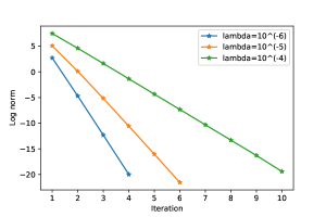
Figure 1: Norm of between the iterations, compared with different values of $\lambda$

Figure1 shows how the difference decrease with the iterations. The smaller the $\lambda$ is chosen, the faster the norm of the difference decreases to $0$. This means that the optimal convergence for $\ll\lambda$ is achieved faster than for high values, closer to the $\lambda$ boundaries.

5 Conclusions

In this paper, a new conceptualization of ensemble training has been presented for the Negative Correlation Extreme Learning Machine (NCELM) model. The training stage can be reformulated as a contraction mapping, and the update of the base learners is seen as a fixed-point iteration. Using Banach theorem, it was proved that the update of the base learners converge to a global optimum, in which error, regularization, and diversity terms from NCELM are optimized altogether.

Besides, this work highlight that reformulation of the training stage as a fixed-point iteration could help in the study of ensemble learning convergence. The re-conceptualization of base learner update in the ensemble as contraction mapping, along with Banach theorem, proves the convergence of the methods, and it is an interesting idea to explore in other ensemble learning methods.

Conflict of interest

The authors declare that they have no conflict of interest.

References

• (1) Arendt, W., Nittka, R.: Equivalent complete norms and positivity. Archiv der Mathematik 92(5), 414–427 (2009)
• (2) Banach, S.: Sur les opérations dans les ensembles abstraits et leur application aux équations intégrales. Fundamenta Mathematicae 3, 133–181 (1922)
• (3) Breiman, L.: Bagging predictors. Machine Learning (1996)
• (4) Chang, P., Zhang, J., Hu, J., Song, Z.: A deep neural network based on elm for semi-supervised learning of image classification. Neural Processing Letters 48(1), 375–388 (2018)
• (5) Chaturvedi, I., Ragusa, E., Gastaldo, P., Zunino, R., Cambria, E.: Bayesian network based extreme learning machine for subjectivity detection. Journal of The Franklin Institute 355(4), 1780–1797 (2018)
• (6) Chen, H., Jiang, B., Yao, X.: Semisupervised Negative Correlation Learning. IEEE Transactions on Neural Networks and Learning Systems 29(11), 5366–5379 (2018)
• (7) Ciesielski, K.: On stefan banach and some of his results. Banach Journal of Mathematical Analysis 1(1), 1–10 (2007)
• (8) Domingos, P.: Why does bagging work? a bayesian account and its implications. In: 3rd International Conference on Knowledge Discovery and Data Mining, pp. 155–158. KDD (1997)
• (9) Freund, Y.: Boosting a weak learning algorithm by majority. Information and Computation (1995). DOI 10.1006/inco.1995.1136
• (10) Girshick, R., Donahue, J., Darrell, T., Malik, J.: Rich feature hierarchies for accurate object detection and semantic segmentation. In: Proceedings of the IEEE Computer Society Conference on Computer Vision and Pattern Recognition (2014)
• (11) Huang, G.B.B., Zhou, H., Ding, X., Zhang, R., Guang-Bin Huang, Hongming Zhou, Xiaojian Ding, Rui Zhang, Huang, G.B.B., Zhou, H., Ding, X., Zhang, R.: Extreme learning machine for regression and multiclass classification. IEEE Transactions on Systems, Man, and Cybernetics, Part B (Cybernetics) 42(2), 513–529 (2012)
• (12) Huanhuan Chen, Xin Yao: Regularized Negative Correlation Learning for Neural Network Ensembles. IEEE Transactions on Neural Networks 20(12), 1962–1979 (2009)
• (13) Kuncheva, L.I., Whitaker, C.J.: Measures of diversity in classifier ensembles and their relationship with the ensemble accuracy. Machine Learning (2003)
• (14) Li, L., Zhao, K., Li, S., Sun, R., Cai, S.: Extreme learning machine for supervised classification with self-paced learning. Neural Processing Letters pp. 1–22 (2020)
• (15) Masoudnia, S., Ebrahimpour, R., Arani, S.A.A.A.: Incorporation of a regularization term to control negative correlation in mixture of experts. Neural processing letters 36(1), 31–47 (2012)
• (16) Mukherjee, I., Rudin, C., Schapire, R.E.: The rate of convergence of AdaBoost. Journal of Machine Learning Research 14, 2315–2347 (2013)
• (17) Parlett, B.: The symmetric eigenvalue problem. Society for Industrial and Applied Mathematics, Philadelphia (1998)
• (18) Perales-González, C., Carbonero-Ruz, M., Pérez-Rodríguez, J., Becerra-Alonso, D., Fernández-Navarro, F.: Negative correlation learning in the extreme learning machine framework. Neural Computing and Applications pp. 1–19 (2020)
• (19) Ren, W., Han, M.: Classification of eeg signals using hybrid feature extraction and ensemble extreme learning machine. Neural Processing Letters 50(2), 1281–1301 (2019)
• (20) Rudin, C., Daubechies, I., Schapire, R.E.: The dynamics of AdaBoost: Cyclic behavior and convergence of margins. Journal of Machine Learning Research (2004)
• (21) Shi, Z., Zhang, L., Liu, Y., Cao, X., Ye, Y., Cheng, M.M., Zheng, G.: Crowd counting with deep negative correlation learning. In: Proceedings of the IEEE conference on computer vision and pattern recognition, pp. 5382–5390 (2018)
• (22) Wang, J., Liu, Z., Wu, Y., Yuan, J.: Mining actionlet ensemble for action recognition with depth cameras. In: Proceedings of the IEEE Computer Society Conference on Computer Vision and Pattern Recognition (2012)
• (23) Wang, S., Chen, H., Yao, X.: Negative correlation learning for classification ensembles. In: International Joint Conference on Neural Networks, pp. 1–8. IEEE (2010)
• (24) Woodbury, M.: Inverting modified matrices. Tech. rep. (1950)
• (25) Wyner, A.J., Olson, M., Bleich, J., Mease, D.: Explaining the success of adaboost and random forests as interpolating classifiers. Journal of Machine Learning Research 18(1), 1558–1590 (2017)
• (26) Xu, X., Deng, J., Coutinho, E., Wu, C., Zhao, L., Schuller, B.W.: Connecting subspace learning and extreme learning machine in speech emotion recognition. IEEE Transactions on Multimedia 21(3), 795–808 (2019)
• (27) Ykhlef, H., Bouchaffra, D.: An efficient ensemble pruning approach based on simple coalitional games. Information Fusion (2017)
• (28) Zhou, X., Xie, L., Zhang, P., Zhang, Y.: An ensemble of deep neural networks for object tracking. In: 2014 IEEE International Conference on Image Processing (ICIP), pp. 843–847. IEEE (2014)
• (29) Zhou, Z.H.: Ensemble methods: Foundations and algorithms (2012)