Late-time description of immiscible Rayleigh-Taylor instability: A lattice Boltzmann study

Abstract

In this paper, the late-time description of immiscible Rayleigh-Taylor instability (RTI) in a long duct is investigated over a comprehensive range of the Reynolds numbers ($1\leq Re\leq 10000$) and Atwood numbers $(0.05\leq A\leq 0.7)$ based on the mesoscopic lattice Boltzmann method. We first reported that the instability with a moderately high Atwood number of 0.7 undergoes a sequence of distinguishing stages at a high Reynolds number, which are termed as the linear growth, saturated velocity growth, reacceleration and chaotic development stages. The spike and bubble at the secondary stage evolve with the constant velocities and their values agree well with the analytical solutions of the potential flow theory. The duration of the spike saturated velocity stage is very shorter than that of the bubble, implying the asymmetric developments between the spike and bubble fronts. Owing to the increasing strengths of the formed vortices, the movements of the spike and bubble are accelerated such that their velocities exceed than the asymptotic values and the evolution of the instability then enters into the reacceleration stage. Lastly, the curves for the spike and bubble velocities have some fluctuations at the chaotic stage and also a complex interfacial structure with large topological change is observed, while it still preserves the symmetry property with respect to the central axis. To determine the nature of the late-time growth, we also calculated the spike and bubble growth rates by using five popular statistical methods and two comparative techniques are recommended, resulting in the spike and bubble growth rates of about 0.13 and 0.022, respectively. When the Reynolds number is gradually reduced, some later stages such as the chaotic and reacceleration stages cannot be reached successively and the structure of the interface in the evolutional process becomes relatively smooth. The influence of the fluid Atwood number is also examined on the late-time RTI development at a large Reynolds number. It is found that the sustaining time for the saturated velocity stage decreases with the Atwood number. The spike late-time growth rate shows an overall increase with the Atwood number, while it has little influence on the bubble growth rate being approximately 0.0215.

I Introduction

The Rayleigh-Taylor instability (RTI) is a fundamental interfacial instability between two fluids that occurs at a perturbed interface when a heavy fluid is supported against gravity by a light fluid. This interesting instability phenomenon can be encountered in cirrus cloud formation, accidental painting technique, and also has many relevant scientific and engineering applications such as geophysics, inertial confinement fusion and astrophysics Zhou1 ; Zhou2 . The pioneering work on the RTI was conducted by Rayleigh and Taylor Rayleigh , who put forward the famous linear stability theory and showed that the RTI amplitude grows exponentially with time. Later, Lewis Lewis experimentally validated the linear stability theory and found that it was effective to describe the interface movement until its amplitude reaching to $0.4$ times the initial wavelength. He also reported that the evolution of the RTI then entered into the nonlinear stage, where the bubble velocity was shown to be proportional to the square root of the gravitational acceleration. The classical linear theory was derived for Euler flows, and numerous subsequent researches have addressed the roles of density difference, viscosity, surface tension and compressibility and the modified linear growth theories including these interwoven factors were deduced Bellman ; Mitchner ; Plesset ; Menikoff . Enlightened by these early works, the RTI subject has nourished the enthusiasm of mathematicians and scientists and interested readers can refer to a good summary of early studies Sharp and the recent reviews Zhou1 ; Zhou2 ; Boffetta ; Livescu on this topic.

Based on initial pattern of the perturbation, the RTI can be divided into the single-mode and multimode Cabot ; Adkins ; Kobayashi instabilities. The single-mode RTI in comparison to the multimode example is simple and ideal, but the study of single-mode phenomenon is still very important not only in its own interests to fluid mechanics, but also that the turbulent growth constant in the multimode instability has a direct relationship with the single-mode terminal velocity Dimonte1 . Besides, the understanding of the single-mode phenomenon can provide good knowledge in the validation of the newly proposed numerical scheme, which thus is the focus of the current study. Following the linear growth stage, the single-mode RTI would evolve with constant velocity, implying that the flow has been transformed into the nonlinear stage. The nonlinear stage has been investigated by many analytical models Layzer ; Alon ; Mikaelian ; Zhang ; Goncharov ; Oron ; Betti ; Sohn ; Banerjee . An important early contribution was attributed to Layzer Layzer , who theoretically analyzed the motion of the fluid-vacuum interface in the gravitational field and proposed the first potential flow model for describing the RTI evolution with limiting Atwood number of 1. Stating from Layzer’s potential flow theory, several analytic formulas were subsequently presented for the nonlinear evolutions of the bubble Alon ; Mikaelian and spike Zhang amplitudes in the single-mode RTI. These models were only applicable to the fluid-vacuum interfaces, and to remove this limitation, Goncharov Goncharov have generalized Layzer’s theory to an improved potential flow model for an arbitrary Atwood number, which predicts the saturated velocities of the inviscid spike $(u_{s})$ and bubble $(u_{b})$ as follows,

$$u_{s}=\sqrt{\frac{2Ag}{(1-A)Ck}},~{}~{}u_{b}=\sqrt{\frac{2Ag}{(1+A)Ck}},$$ (1)

where $A$ is the Atwood number, $k$ is the perturbation wave number, $g$ is the gravitational acceleration, $C$ is a constant given by 1 or 3 for the two-dimensional or three-dimensional geometry. An alternative heuristic approach for describing the bubble and spike saturated velocities was proposed by Oron et al. Oron , who constructed the buoyancy-drag model, interestingly yielding the identical results to the potential flow approach of Goncharov Goncharov . Further, Betti and Sanz Betti have examined the effect of the vorticity accumulation inside the bubble on the nonlinear evolution of ablative single-mode RTI, and the resulting bubble saturated velocity including the vorticity effect was formulated. It is noticed that the viscosities of the fluids are neglected in above potential flow models. Sohn Sohn and Banerjee Banerjee then analyzed the role of viscosity and anticipated the increased skin-friction drag between viscous bubble and spike. To this end, the modified potential flow models combining the viscosity effect and the vorticity Banerjee or the surface tension force Sohn were established for saturated velocity stage.

In addition to these theoretical studies, several researchers attempt to describe the nonlinear evolutional stages of the single-mode RTI using the experimental and numerical approaches. Waddell et al. Waddell experimentally investigated the two-dimensional single-mode RTI in low Atwood number fluid systems and reported that the initial growth rate agrees well with linear stability theory. Additionally, they observed that average of the late-time spike and bubble velocities approaches to a constant. Glimm et al. Glimm used the front-tracking method to carry out a long simulation of the two-dimensional single-mode RTI with a moderate Atwood number. They found that the saturated velocity stage with a constant velocity breaks down at late time followed by a new phenomena that the spike velocity was accelerated, indicating a reacceleration process after a plateau time. The reacceleration stage was also confirmed in the numerical simulation of the single-mode RTI with low or moderate density difference Ramaprabhu and the experiment in a low Atwood number system Wilkison . The reason for the reacceleration behavior was ascribed to the formation of the vortices on the bubble-spike interfaces induced by the Kelvin-Helmholtz (KH) instability. Ramaprabhu et al. Ramaprabhu1 further conducted a longer simulation in order to explore the late-time behaviours of the single-mode RTI, and first summarized the stability with low Atwood numbers and large Reynolds numbers would undergo four different stages known as the linear growth, saturated velocity growth, reacceleration, and chaotic mixing stages. During the chaotic mixing stage, the bubble and spike velocities experience an eventual decrease lower than the saturated velocity of the potential flow model Goncharov and the symmetries within the bubble and spike images were broken in their simulations. However, the later direct numerical simulations Wei indicated that the late-time bubble at high Reynolds number maintains a symmetric pattern and its growth exhibits a mean quadratic law. This late-time quadratic growth phenomenon was also observed in our mesoscopic numerical simulations of the single-mode RTI for low and moderate Atwood numbers Liang1 ; Liang2 . Recently, Hu et al. Hu1 numerically investigated the two-dimensional single-mode RTI with a low Atwood number and found that the bubble velocity for medium Reynolds numbers was decelerated and accelerated repeatedly after the reacceleration stage, they called this stage as the deceleration-acceleration stage. More recently, Bian et al. Bian conducted a detailed study on the growth of compressible single-mode RTI at different Reynolds numbers and Atwood numbers, and found that for a sufficiently high Reynolds number, the bubble late-time acceleration is persistent and does not vanish, which is consistent with the direct numerical results of incompressible RTI Wei .

As reviewed above, there have been some numerical works Ramaprabhu1 ; Wei ; Liang1 ; Liang2 ; Hu1 ; Bian to investigate the late-time single-mode RTI, which provide a good understanding of this complex interfacial instability phenomenon. However, most of these studies Wei ; Liang1 ; Liang2 ; Hu1 only focus on the low Atwood number fluid systems, and the instability durations in all reported simulations are relatively short (the aspect ratio of the two-dimensional computational domain does not exceed than 8). Actually, it needs a longer vertical domain for the flow to reach the late-time stage for a high Atwood number. In addition, the quantitative description on the late-time growth of the single-mode RTI is still very lacking. To fill this gap, we invoked an improved mesoscopic lattice Boltzmann algorithm Liang3 to systematically explore the late-time dynamics of the single-mode RTI in an elongated duct with an aspect ratio of 15, and the influences of wide Reynolds numbers and Atwood numbers are investigated in detail. The rest of this article is organized as follows. In Sec. II, we will give a brief introduction of the used numerical methods. Sec III describes the long-time evolution of single-mode instability with different Reynolds numbers and Atwood numbers. Finally, we conduct a summary in Sec. IV.

II Mathematical method

The phase-field model Jacqmin ; Shen has recently received great attention in simulating multiphase flows due to its firm physics for describing interfacial dynamics. In this model, an order parameter is introduced to identify different phases, and the interface is assumed as the transition region of finite thickness where the physical variables are smoothly distributed. This feature makes it become advantageous for tackling interfacial flows involving large topological change. Considering the space $\Omega$ occupied by a multiphase system, the total free-energy functional of a multiphase system can be expressed by Jacqmin ,

$$E=\int_{\Omega}[F(\phi)+{\frac{k}{2}|\nabla\phi|^{2}}]d\Omega,$$ (2)

where $\phi$ is an order parameter, $F(\phi)$ is the bulk free-energy density taking the form of the double-well potential $F(\phi)=\beta\phi^{2}(1-\phi)^{2}$, ${\frac{k}{2}|\nabla\phi|^{2}}$ accounts for the excess free energy in the interfacial region, the parameters $k$, $\beta$ depend on the surface tension $\sigma$ and the interface width $D$ by $D=\sqrt{8k/\beta}$, $\sigma=\sqrt{2k\beta}/6$. The Cahn-Hilliard model admits the energy dissipation law and is viewed as a gradient flow with respect to the free-energy functional Shen . In this case, the chemical potential can be defined as the variation of total free-energy functional (2),

$$\mu=4\beta\phi(\phi-1)(\phi-\frac{1}{2})-k{\nabla^{2}}\phi,$$ (3)

and then the classical Cahn-Hilliard equation for governing the order parameter can be expressed by

$${{\partial\phi}\over{\partial t}}+\nabla\cdot(\phi{\bf{u}})=\nabla\cdot{M}(\nabla{\mu}),$$ (4)

where ${\bf{u}}$ is the fluid velocity, $M$ is the mobility. To simulate interfacial flows, the Cahn-Hilliard equation should be coupled with the incompressible Navier-Stokes equations including the surface tension (${\mathbf{F}}_{s}$) and external forces ($\mathbf{G}$),

$$\nabla\cdot{\bf{u}}=0,$$ (5a)

$$\rho({{\partial{\bf{u}}}\over{\partial t}}+{\bf{u}}\cdot\nabla{\bf{u}})=-\nabla p+\nabla\cdot\left[{\nu\rho(\nabla{\bf{u}}+\nabla{{\bf{u}}^{T}})}\right]+{{\bf{F}}_{s}}+{\bf{G}},$$ (5b)

where $\rho$ is the fluid density, $p$ is the hydrodynamic pressure, $\nu$ is the kinematic viscosity. To achieve a low spurious velocity, we choose the potential form of the surface tension force $\mathbf{F}_{s}=\mu\nabla{\phi}$ Jacqmin .

To solving the coupled system of the Cahn-Hilliard and Navier-Stokes equations, some mesoscopic lattice Boltzmann algorithms Liang1 ; Zu ; Liang4 have been reported, among which an improved one Liang1 is utilized to investigate the variable-density RTI owing to its great potential in solving complex interfacial instability Liang5 . The mesoscopic algorithm takes advantages of double distribution functions and their evolutional equations equipped with an advanced multiple-relaxation-time collision operator can be written as Guo

$${f}_{i}({\bf{x}}+{{\bf{c}}_{i}}{\delta_{t}},t+{\delta_{t}})-{f}_{i}({\bf{x}},t)=-({\bf{M}}^{-1}{\bf{S}}_{f}{\bf{M}})_{ij}[{{f}_{j}({\bf{x}},t)-f_{j}^{eq}({\bf{x}},t)}]+{\delta_{t}}[\mathbf{M}^{-1}(\mathbf{I}-\frac{\mathbf{S}_{f}}{2})\mathbf{M}]_{ij}{F_{j}({\bf{x}},t)},$$ (6a)

$${g}_{i}({\bf{x}}+{{\bf{c}}_{i}}{\delta_{t}},t+{\delta_{t}})-{g}_{i}({\bf{x}},t)=-({\bf{M}}^{-1}{\bf{S}}_{g}{\bf{M}})_{ij}[{{g}_{j}({\bf{x}},t)-g_{j}^{eq}({\bf{x}},t)}]+{\delta_{t}}[\mathbf{M}^{-1}(\mathbf{I}-\frac{\mathbf{S}_{g}}{2})\mathbf{M}]_{ij}{G_{j}({\bf{x}},t)},$$ (6b)

where ${f}_{i}({\bf{x}},t)$ and ${g}_{i}({\bf{x}},t)$ are the particle distribution functions at position $\mathbf{x}$ and time $t$, $f_{i}^{eq}({\bf{x}},t)$ and $g_{i}^{eq}({\bf{x}},t)$ are the equilibrium distribution functions, ${\bf{c}}_{i}$ is the discrete velocity, ${\bf{M}}$ is collision matrix, ${\bf{S}}_{f}$ and ${\bf{S}}_{g}$ are the diagonal relaxation matrices, $F_{i}({\bf{x}},t)$ and $G_{i}({\bf{x}},t)$ are the distribution functions of source term and forcing term, respectively. To be consistent with the target equations, the equilibrium distributions are designed as Liang1

$$f_{i}^{eq}=\left\{\begin{array}[]{ll}\phi+({\omega_{i}}-1)\eta\mu,&\textrm{ $i=0$},\\ {\omega_{i}}\eta\mu+{\omega_{i}}\phi{{{\bf{c}}_{i}\cdot{\bf{u}}}\over{c_{s}^{2}}},&\textrm{ $i\neq 0$}\\ \end{array}\right.$$ (7)

and

$$g_{i}^{eq}=\left\{\begin{array}[]{ll}{p\over{c_{s}^{2}}}({\omega_{i}}-1)+\rho{s_{i}}({\bf{u}}),&\textrm{ $i=0$},\\ {p\over{c_{s}^{2}}}{\omega_{i}}+\rho{s_{i}}({\bf{u}}),&\textrm{ $i\neq 0$}\\ \end{array}\right.$$ (8)

with

$${s_{i}}({\bf{u}})={\omega_{i}}\left[{{{{{\bf{c}}_{i}}\cdot{\bf{u}}}\over{c_{s}^{2}}}+{{{{({{\bf{c}}_{i}}\cdot{\bf{u}})}^{2}}}\over{2c_{s}^{4}}}-{{{\bf{u}}\cdot{\bf{u}}}\over{2c_{s}^{2}}}}\right],$$ (9)

where $\eta$ is a free parameter that controls the mobility, $c_{s}$ is the sound speed, and $\omega_{i}$ is the weighting coefficient. For two-dimensional flows, we apply the popular $D2Q9$ discrete-velocity model YWei1 ; Chai ; YWei2 to the lattice Boltzmann algorithm, where the weighting coefficient $\omega_{i}$ is given by $\omega_{0}=4/9$, $\omega_{1-4}=1/9$ and $\omega_{5-8}=1/36$, and the discrete velocity ${\bf{c}}_{i}$ is defined by

$$\mathbf{c}_{i}=\left\{\begin{array}[]{ll}(0,0)c,&\textrm{ $i=0$},\\ (\cos[(i-1)\pi/2],\sin[(i-1)\pi/2])c,&\textrm{ $i=1-4$},\\ \sqrt{2}(\cos[(i-5)\pi/2+\pi/4],\sin[(i-5)\pi/2+\pi/4])c,&\textrm{ $i=5-8$},\end{array}\right.$$ (10)

where $c=\delta_{x}/\delta_{t}$, $\delta_{x}$ and $\delta_{t}$ are the lattice length and time step respectively, and $c_{s}=c/\sqrt{3}$. In the multiphase lattice Boltzmann method, $\delta_{x}$ and $\delta_{t}$ are conventionally set to be length and time units, i.e., $\delta_{x}=\delta_{t}=1.0$. The corresponding collision matrix $\bf{M}$ for the $D2Q9$ model is given as Lallemand

$$\bf{M}=\left(\begin{array}[]{rrrrrrrrr}1&1&1&1&1&1&1&1&1\\ -4&-1&-1&-1&-1&2&2&2&2\\ 4&-2&-2&-2&-2&1&1&1&1\\ 0&1&0&-1&0&1&-1&-1&1\\ 0&-2&0&2&0&1&-1&-1&1\\ 0&0&1&0&-1&1&1&-1&-1\\ 0&0&-2&0&2&1&1&-1&-1\\ 0&1&-1&1&-1&0&0&0&0\\ 0&0&0&0&0&1&-1&1&-1\end{array}\right),$$

which is used to transform the particle distribution functions into their corresponding moments. With some algebraic manipulations, the equilibrium distribution functions in the moment space can be given by

$$\mathbf{m}^{eq}_{f}=(\phi,-4\phi+2\eta\mu,4\phi-3\eta\mu,\phi u_{x},-\phi u_{x},\phi u_{y},-\phi u_{y},0,0)$$ (11a)

$$\mathbf{m}^{eq}_{g}=(0,6p+3\rho|\mathbf{u}|^{2},-9p-3\rho|\mathbf{u}|^{2},\rho u_{x},-\rho u_{x},\rho u_{y},-\rho u_{y},\rho(u_{x}^{2}-u_{y}^{2}),\rho u_{x}u_{y})$$ (11b)

where $u_{x}$, $u_{y}$ are the horizontal and vertical components of velocity. The relaxation matrices of ${\bf{S}}_{f}$ and ${\bf{S}}_{g}$ in Eqs. (6a) and (6b) are defined by

$${\mathbf{S}}_{f}=diag(s_{0}^{f},s_{1}^{f},s_{2}^{f},s_{3}^{f},s_{4}^{f},s_{5}^{f},s_{6}^{f},s_{7}^{f},s_{8}^{f}),$$ (12)

$${\mathbf{S}}_{g}=diag(s_{0}^{g},s_{1}^{g},s_{2}^{g},s_{3}^{g},s_{4}^{g},s_{5}^{g},s_{6}^{g},s_{7}^{g},s_{8}^{g}),$$ (13)

where $0<s_{i}^{f}<2,0<s_{i}^{g}<2$. Another indispensable event in the lattice Boltzmann approach is to design a suitable forcing distribution function since the discrete lattice effect could be induced when the source or forcing term is incorporated. Previously, Liang et al. Liang1 considered the discrete lattice effect and added the time derivative term into the source distribution function

$$F_{i}=\frac{\omega_{i}\mathbf{c}_{i}\cdot\partial_{t}(\phi\mathbf{u})}{c_{s}^{2}}$$ (14)

and also in order to recover the incompressible Navier-Stokes equations correctly, the forcing distribution function $G_{i}$ in Eq. (6b) is defined by Liang1

$${{G}_{i}}=\frac{(\mathbf{c}_{i}-\mathbf{u})}{c_{s}^{2}}\cdot[s_{i}(\mathbf{u})\nabla(\rho{c_{s}^{2}})+(\mathbf{F}_{s}+\mathbf{F}_{a}+\mathbf{G})(s_{i}(\mathbf{u})+\omega_{i})],$$ (15)

where $\mathbf{F}_{a}$ is an additional interfacial force given by $\mathbf{F}_{a}=\frac{d\rho}{d\phi}M\nabla^{2}\mu\mathbf{u}$. The macroscopic quantities $\phi$, $\bf{u}$ and $p$ can be obtained by calculating zeroth- or first-order moments of the particle distribution functions,

$$\phi=\sum\limits_{i}{{f_{i}}},$$ (16a)

$$\rho{\bf{u}}={{\sum\limits_{i}{{{\bf{c}}_{i}}{g_{i}}}+\frac{{\delta_{t}}}{2}({{\bf{F}_{s}}+\mathbf{F}_{a}+\mathbf{G}})}},$$ (16b)

$$p={{c_{s}^{2}}\over{(1-{\omega_{0}})}}[{\sum\limits_{i\neq 0}{{g_{i}}}+{{{\delta_{t}}}\over 2}{\bf{u}}\cdot\nabla\rho+\rho{s_{0}}(\textbf{u})}],$$ (16c)

and the macroscopic density $\rho$ is determined by a linear differential function with respect to the order parameter,

$$\rho=\phi(\rho_{h}-\rho_{l})+\rho_{l},$$ (17)

where $\rho_{h}$ and $\rho_{l}$ are the densities of the heavy and light fluids. Applying the Chapman-Enskog procedure, the used lattice Boltzmann method can recover the exact Cahn-Hilliard and Navier-Stokes coupled equations with the mobility $M$ and the kinematic viscosity $\nu$ given by

$$M=\eta c_{s}^{2}(\tau_{f}-0.5)\delta_{t}.$$ (18a)

$$\nu=c_{s}^{2}(\tau_{g}-0.5)\delta_{t},$$ (18b)

where $1/\tau_{f}=s_{3}^{f}=s_{5}^{f}$, and $1/\tau_{g}=s_{7}^{g}=s_{8}^{g}$. In our simulations, the relation $s_{0}^{g}=s_{3}^{g}=s_{5}^{g}=1.0$ is used, $s_{7}^{g}$ and $s_{8}^{g}$ are adjusted according to the value of the Reynolds number. The remaining relaxation parameters in Eq. (13) are chosen as $s_{1}^{g}=s_{2}^{g}=1.0$ and $s_{4}^{g}=s_{6}^{g}=1.7$, while all the relaxation factors $s_{i}^{f}$ in Eq. (12) are given as 1.0. Besides, in the practical applications, the temporal and spacial derivatives need to be numerically calculated, here we adopt the explicit Euler scheme to compute the time derivative, i.e., $\partial_{t}(\phi\mathbf{u})=[\phi(t)\mathbf{u}(t)-\phi(t-\delta_{t})\mathbf{u}(t-\delta_{t})]/\delta_{t}$, and the spacial gradient terms are discretized by a second-order isotropic central schemes,

$$\nabla\chi({\bf{x}})=\sum\limits_{i\neq 0}{\frac{\omega_{i}\textbf{c}_{i}\chi({\bf{x}}+{{\bf{c}}_{i}}{\delta_{t}})}{c_{s}^{2}\delta_{t}}}$$ (19)

$$\nabla^{2}\chi({\bf{x}})=\sum\limits_{i\neq 0}{\frac{2\omega_{i}[\chi({\bf{x}}+{{\bf{c}}_{i}}{\delta_{t}})-\chi({\bf{x}})]}{c_{s}^{2}\delta_{t}^{2}}},$$ (20)

where $\chi$ represents an arbitrary variable that the derivative operator has been applied.

III Numerical Results and Discussions

To reach the late-time stage for a high Atwood number, we consider the evolution of the single-mode instability in a sufficiently long rectangular pipe divided by an even mesh of $L\times W=8160\times 544$, which has already given the grid-independent results. Initially, a small cosine perturbation is seeded on the central section of the rectangle and then the initial phase interface is located at

$$h(x,y)=0.5L+0.05W\cos(k\pi),$$ (21)

where the wave number $k$ is defined by $k=2\pi/W$. To match the pattern of the interface, the initial distribution for the order parameter is given by

$$\phi(x,y)=0.5+0.5\tanh\frac{2[y-h(x,y)]}{D},$$ (22)

where the interface thickness $D$ is set to be four lattice units, and the surface tension $\sigma$ is fixed as $5\times 10^{-5}$. As is well known, the behaviour of the single-mode instability can be characterized by two important dimensionless numbers, i.e., the Reynolds number ($Re$) and the Atwood number($A$), which are defined as follows Hex ,

$$Re=\frac{W\sqrt{gW}}{\nu},~{}~{}A=\frac{\rho_{h}-\rho_{l}}{\rho_{h}+\rho_{l}},$$ (23)

where $\nu$ is the kinematic viscosity. To incorporate the gravitational effect, the following buoyancy force $\mathbf{G}$ in the vertical direction is applied to binary fluids,

$$\mathbf{G}=[0,-(\rho-\frac{\rho_{h}+\rho_{l}}{2})g].$$ (24)

In the simulations, the density of the heavy fluid ($\rho_{h}$) is set as 1.0 and the density for the light fluid ($\rho_{l}$) can be determined by a given Atwood number. The gravitational acceleration is chosen to satisfy the relation $\sqrt{gW}=0.04$ and the Peclet number $(Pe)$ determining the value of the mobility is fixed as 50 based on the definition $Pe=\sqrt{gW}D/M\beta$ Zu . The periodic boundary conditions are applied in the horizontal direction, while the halfway bounce-back scheme is used on the upper and lower boundaries. In this study, the characteristic length is chosen as the the wavelength of the perturbation $W$, $\sqrt{gW}$ is regarded as the characteristic velocity, and then the characteristic time is defined by $\sqrt{W/g}$. The present definitions of the characteristic velocity and time are different from the ones $\sqrt{\frac{AgW}{1+A}}$ and $\sqrt{\frac{(1+A)W}{Ag}}$ used in previous literatures Wei ; Hu1 , which obviously depend on the studied density difference of two fluids and would be unreasonable from the perspective of physics. In addition, we would like to stress that the relevant statistics presented below have been normalized by these characteristic values.

III.1 Effect of the Reynolds number

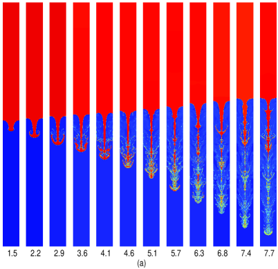
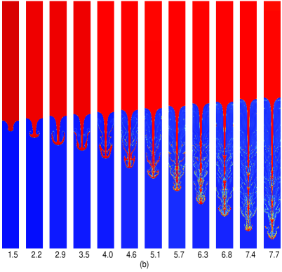
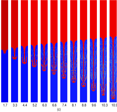
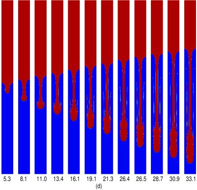
Figure 1: The time evolutions of the interfacial patterns in the immiscible RTI $(A=0.7)$ with different Reynolds numbers: (a) $Re=10000$, (b) $Re=1000$, (c) $Re=100$, and (d) $Re=10$.

The effect of the Reynolds number is first investigated on the late-time dynamics of the single-mode RTI at a moderately high Atwood number of 0.7. We simulated the evolution of the single-mode instability within a comprehensive range of Reynolds numbers from 1 to 10000 and the snapshots of interfacial patterns under four typical Reynolds numbers are displayed in Fig. 1. From this figure, it can be observed that the instability in regardless of various Reynolds numbers exhibits similar interfacial dynamics at the initial stage: the heavy and light fluids seep into each other forming into the spike and bubble structures. In the following, the spike and bubble display the distinct behaviours at different Reynolds numbers. For high Reynolds number of 10000, the spike continues to fall down and the bubble rises up accompanied by the occurrence of the nonlinear effect, which begins to affect the bubble and spike dynamics. It is seen that the spike rolls up at its front creating a pair of vortices due to the appearance of the nonlinear KH instability caused by the velocity difference on the bubble-spike interface. Then these two vortices grow in size and the increasing nonlinear KH instability provides the rolling motion of the interface, resulting in a pair of secondary vortices at the tails of the roll-ups. As time progresses, the interaction between fluids in the mixing region becomes more and more intensive, which leads to the roll-ups of the interfaces at the multiple positions and eventually induces the formation of a chaotic interfacial structure with large topological change. Nonetheless, the close inspection showed that the late-time symmetries of the spike or bubble images at a moderately high Atwood number can be still preserved familiar from our low-Atwood-number results Liang1 ; Liang2 , which is also qualitatively consistent with the high-resolution direct numerical simulations of miscible single-mode RTI Wei ; Bian . As the Reynolds number is reduced, the roll-up phenomenon appears at a later time and the vortical sizes are accordingly smaller. In general, the structure of the interface in the evolutional process becomes relatively smooth due to the more stabilized shear layer between bubble and spike. Specially, the heavy fluid at a extremely small Reynolds number of 10 falls down continuously in the manner of the spike almost without the occurrence of the roll-up or breakup behavior.

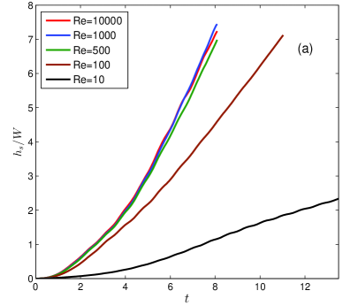
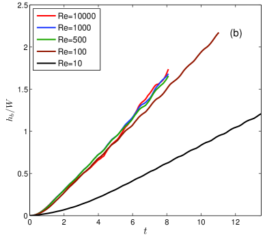
Figure 2: Time variations of (a) normalized spike amplitude and (b) normalized bubble amplitude in the immiscible RTI with various Reynolds numbers.

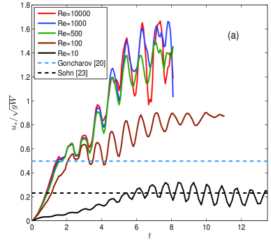
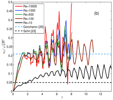
Figure 3: Time variations of (a) normalized spike velocity and (b) normalized bubble velocity in the immiscible RTI with various Reynolds numbers.

Further, we quantitatively examined the effect of the Reynolds number on the instability growth in terms of the spike and bubble amplitudes and velocities, which are often the focuses of the previous studies on the single-mode RTI  Waddell ; Goncharov ; Wilkison ; Liang2 ; Wei . The spike and bubble amplitudes marked by $h_{s}$ and $h_{b}$ are defined as the vertical distances between the spike/bubble fronts and their corresponding initial positions such that the amplitudes for the spike and bubble at initial time are zero, while their evolutional velocities denoted by $u_{s}$ and $u_{b}$ are calculated from the amplitude profiles by the time derivatives of the amplitudes $h_{s}$, $h_{b}$. Figures 2(a) and 2(b) show the time variations of the spike and bubble normalized amplitudes with a comprehensive range of Reynolds numbers. It can be found that for all Reynolds numbers, both the spike and bubble amplitudes increase with time and also achieve greater values at a higher Reynolds number, while the degree of increase is weakened and even the amplitude curves have no obvious differences when the Reynolds number exceeds a certain value. This indicates that the Reynolds number effect becomes no longer important when its value is high enough. To further illustrate this statement, we also conduct a theoretical analysis on the growth of the single-mode instability. The dynamics of the spike front in the incompressible RTI can be described by a balance per unit mass of the buoyant and dissipation forces Abarzhi

$$\frac{dh_{s}}{dt}=u_{s},~{}~{}~{}~{}~{}\frac{du_{s}}{dt}=Ag+F_{d}$$ (25)

where $F_{d}$ is the dissipation force defined as the rate of momentum loss in the direction of gravity $F_{d}=-\varepsilon/\nu$, $\varepsilon$ is the energy dissipation rate. Neglecting the viscous time scale, the dimensional grounds conducted by Sreenivasan Sreenivasan suggest that the energy dissipation rate can be expressed as $\varepsilon=C_{e}\nu^{3}/W$, where $C_{e}$ is a positive constant. Substituting the formula into Eq. (25), one can find that a smaller dissipation force accelerating the spike growth can be achieved in theory for a larger Reynolds number. Furthermore, when the Reynolds number is sufficiently large, the dissipation force becomes extremely small, in this case the gravitational force dominates over the dissipation force such that the change in fluid viscosity has no significant influence on the spike development. This theoretical analysis can be well confirmed in our numerical experiments, where the spike and bubble amplitudes indeed increase with the Reynolds number at first and then almost are independence of the sufficiently high Reynolds number. In addition, the comparison between the spike and bubble amplitude curves implies that the spike front grows more quickly than that of the bubble. The time evolutions of the spike and bubble velocities with these typical Reynolds numbers are also measured in Figs. 3(a) and 3(b). From these figures, we identified the distinct growth stages as describing the evolution of single-mode instability with a moderately large Atwood number at different Reynolds numbers. For high or medium Reynolds numbers, the development of the single-mode RTI experiences four distinguishing stages named as the linear growth, saturated velocity growth, reacceleration, and chaotic growth stages. At the linear stage, the perturbation grows with an exponential function Waddell followed by the saturated velocity growth stage, where the bubble and spike evolve with constant velocities, as can be clearly seen in Figs. 3(a) and 3(b). For comparisons, the analytical potential flow model by Goncharov Goncharov for predicting the spike and bubble saturated velocities given in Eq. (1) is also presented. It can be found that the present numerical results quantitatively agree well with the corresponding analytical solutions. Besides, the duration of the saturated velocity growth stage for the spike in the relatively high-Atwood-number RTI is shown to be transient compared with the case of the low-Atwood-number Liang1 ; Wei , which was also observed in the numerical simulation of single-mode RTI with a moderate Atwood number Goncharov . As for the bubble, its lasting time of this stage is found to be longer than that of the spike. After the saturated velocity stage, the increasing nonlinear strength of vortices in the proximities of the spike and bubble tips accelerates the growths of the spike and bubble, making their evolutional velocities exceed the values of the potential flow theory Goncharov , which indicates that the instability has entered into the reacceleration stage. The reacceleration stage cannot last indefinitely. From Figs. 3(a) and 3(b), it can be shown that the spike and bubble velocities at the late time become unstable and are accelerated and decelerated repeatedly, suggesting the evolution of the stability has been transformed into the chaotic development stage. The chaotic stage was primarily found by Ramaprabhu et al. Ramaprabhu1 using the integrated large eddy simulation, while different from the present observation, they reported that the spike and bubble velocities at the chaotic stage showed an decrease with time probably owning to the low resolution of the adopted computational grid. Actually, the fluctuation behaviors for the spike and bubble velocities were also observed in the high-resolution direct numerical simulations Wei ; Hu1 ; Bian and our mesoscopic lattice Boltzmann simulations Liang1 ; Liang2 for low Atwood number fluid system. As the Reynolds number is gradually reduced, we can observe from Figs. 3(a) and 3(b) that some later stages such as the reacceleration and chaotic development stages cannot be reached successively. For instance, the bubble and spike evolutional velocities at a low Reynolds number of 10 are observed to have initially slight fluctuations at the late time and eventually approach the quasisteady values without the appearances of the reacceleration and chaotic stages. In addition, it is noted that the spike and bubble quasisteady velocites are smaller than the solutions of the potential flow theory owing to the neglected viscosity effect in his analysis Goncharov . Sohn Sohn realized this problem and modified the asymptotic bubble velocity including the viscosity and surface tension force effects as

$$u_{b}=\sqrt{\frac{2Ag}{3(1+A)k}-\frac{k\sigma}{9\rho_{h}}+\frac{4}{9}k^{2}\nu^{2}}-\frac{2}{3}k\nu,$$ (26)

and the corresponding spike asymptotic velocity inspired by the work of Goncharov Goncharov can be written as

$$u_{s}=\sqrt{\frac{2Ag}{3(1-A)k}-\frac{k\sigma}{9\rho_{h}}+\frac{4}{9}k^{2}\nu^{2}}-\frac{2}{3}k\nu.$$ (27)

We also plotted in Figs. 3(a) and 3(b) the above theoretical solutions of the spike and bubble asymptotic velocities at a low Reynolds number of 10. It can be found that the numerical prediction of the spike velocity at the saturated velocity stage agrees well with the theoretical solution, while the numerical result for the bubble saturated velocity is higher than the corresponding theoretical solution. This discrepancy may be caused by the effect of some inapparent vortices Betti and needs to be deeply investigated in future research.

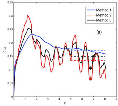
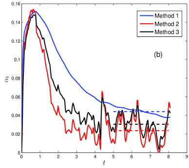
Figure 4: Time variations of (a) spike and (b) bubble normalized accelerations computed by Methods 1, 2 and 3. The dotted lines represent the averages of the spike and bubble accelerations at the later period.

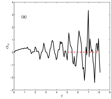
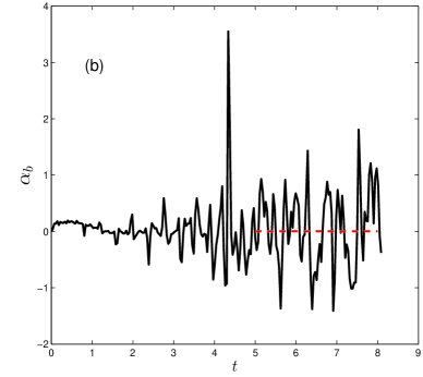
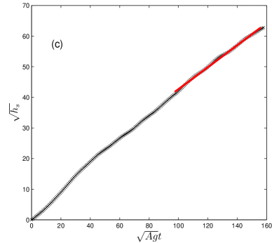
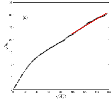
Figure 5: Time variations of (a) spike and (b) bubble normalized accelerations computed by Method 4 and the dotted lines are the averaging values at the later stage. The dependence of (c) $\sqrt{h_{s}}$ and (d) $\sqrt{h_{b}}$ on the variable $\sqrt{Ag}t$ by Method 5 and the solid lines represent their late-time linear fitting curves.

Based on the latest knowledge Wei ; Liang2 ; Bian , it has been recognized that the late-time growth of the single-mode RTI with high Reynolds numbers exhibits a mean quadratic law in the terms of

$$h_{s,b}=\alpha_{s,b}gAt^{2},$$ (28)

where $h_{s,b}$ with the subscripts $s$ and $b$ represent the spike and bubble amplitudes, and $\alpha_{s,b}$ are the corresponding spike and bubble growth rates. To determine the late-time growth nature of the single-mode RTI with a moderately high Atwood number, we also measured the spike and bubble growth rates at a high Reynolds number of 10000. To data, there have been several statistical approaches to compute the growth rate coefficients of the multi-mode phenomenon, which will be adopted here to derive the spike and bubble late-time growth rates of single-mode instability and the comprehensive comparisons of these statistical methods are also conducted. Based on their basic definitions given in Eq. (28), the coefficients reflecting the spike and bubble growth rates can be calculated via the following relation Cabot

$${\alpha_{s,b}}={\frac{h_{s,b}}{Agt^{2}}}.$$ (29)

Ristorcelli et al. Ristorcelli and Cook et al. Cook using completely different approaches, deduced the same formula for computing the spike and bubble growth rates, which can be expressed as

$$\alpha_{s,b}={\frac{{{\dot{h}}_{s,b}}^{2}}{4Agh}},$$ (30)

where ${\dot{h}}_{s,b}$ with the subscripts $s$ and $b$ respectively denote the time derivatives of the spike and bubble amplitudes. To achieve a better convergence, Clark Clark also proposed another measurement method to obtain the spike and bubble growth rates,

$${\alpha_{s,b}}={\frac{\partial{h_{s,b}}}{\partial{Z}}}={\frac{\partial{h_{s,b}}}{\partial{z}}}{\frac{\partial{z}}{\partial{Z}}}={\frac{1}{2A}\frac{\partial{h_{s,b}}}{\partial{z}}},$$ (31)

where $Z=2Az$, $z={gt^{2}/2}$, $t$ is the time that the acceleration is applied. In addition, Wei et al. Wei presented a direct statistical manner to determine the spike and bubble growth rates,

$$\alpha_{s,b}={\frac{{{\ddot{h}}_{s,b}}}{2Ag}},$$ (32)

where ${{\ddot{h}}_{s,b}}$ are the second derivatives of the spike and bubble amplitudes with respect to the evolutional time. Recently, Olson and Jacobs Olson took the square root of Eq. (28) yielding a linear function in time,

$$h^{1/2}_{s,b}={({\alpha_{s,b}}Ag)^{1/2}}t,$$ (33)

thus the coefficients $\alpha_{s,b}$ can be easily extracted by plotting the linear fitting curves of $h^{1/2}_{s,b}$ versus $(Ag)^{1/2}t$ at the late time. Most of these statistical methods are proposed in order to calculate the growth coefficients of the multi-mode instability with an exception Wei . Although they seem to be significantly different in form, they are mathematically equivalent but could produce distinct behaviours of growth rate curves in practical applications Cabot ; Akula . For the convenience of the discussion, the aforementioned five statistical methods given in Eq. (29) to (33) are orderly labeled as Method 1 to 5. Figure 4 depicts the time evolutions of the spike and bubble accelerations computed directly from Methods 1, 2 and 3. It can be seen that the spike and bubble normalized accelerations by Method 1 approximate to nearly constant values with slight reductions by the end of the simulation, while the predictions of the spike and bubble accelerations by Methods 2 and 3 have some fluctuations at the late-time stage. We conducted the late-time averages of these acceleration curves to obtain the spike and bubble growth rates, and the measured results are summarized in Table 1. It is shown that the spike growth rates $\alpha_{s}$ by Methods 1, 2 and 3 are 0.1705, 0.1337 and 0.1483 respectively, while the corresponding bubble growth rates $\alpha_{b}$ are 0.0441, 0.0236 and 0.0305. Further, we also presented the snapshots of the spike and bubble standardized accelerations obtained by Method 4 in Figs. 5(a) and 5(b), and find that the growth rates fluctuate around the mean values of 0.0157 and 0.0017, respectively. In addition, the relations between $\sqrt{h_{s,b}}$ and $\sqrt{Ag}t$ are plotted in Figs. 5(c) and 5(d), where the linear fitting curves at the late time are also presented, indicating the measured spike and bubble growth rates $\alpha_{s}$ and $\alpha_{b}$ as 0.1289 and 0.0207, respectively. Though the comparisons of these predicted growth rates in Table 1, it can be found that the result of Method 4 is far less than those of other four statistical methods, which thus is not a good choice in the measurements of the late-time growth rates. Meanwhile, the largest values for the growth rates achieved by Method 1 would also be not applied, and the prediction of the bubble growth rate by Method 3 is relatively high. In general, the results of Methods 2 and 5 are close to each other and will be recommended in the following calculations of the spike and bubble growth rates with various Atwood numbers. As we noted, it has been reported that Methods 2 and 5 also produced the comparative results in predicting the growth rates of multi-mode RTI and would be the preferred choices Akula .

Table 1: The measured spike and bubble growth rates $\alpha_{s}$ and $\alpha_{b}$ using five statistical methods

Statistical method	$\alpha_{s}$	$\alpha_{b}$
Method 1	0.1705	0.0441
Method 2	0.1337	0.0236
Method 3	0.1483	0.0305
Method 4	0.0157	0.0017
Method 5	0.1289	0.0207

III.2 Effect of the Atwood number

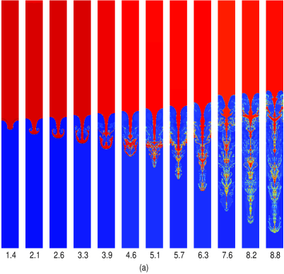
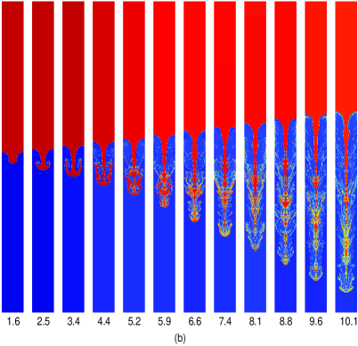
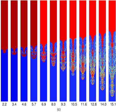
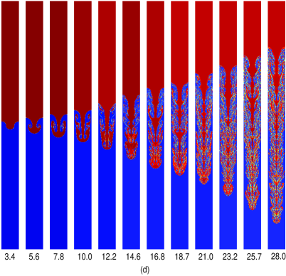
Figure 6: Time evolutions of the interfacial patterns in the immiscible RTI $(Re=10000)$ with different Atwood numbers: (a) $A=0.6$, (b) $A=0.5$, (c) $A=0.3$, and (d) $A=0.1$.

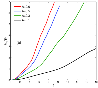
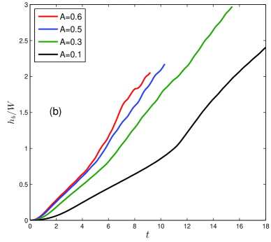
Figure 7: Time variations of (a) normalized spike amplitude and (b) normalized bubble amplitude in the immiscible RTI with various Atwood numbers.

In this subsection, we will conduct a late-time description of single-mode RTI with an extensive range of Atwood numbers under the circumstance of a sufficiently high Reynolds number of 10000. Figure 6 depicts the time evolutions of the density visualizations at four different Atwood numbers. It can be found that for all Atwood numbers, a heavy fluid and a light one penetrate into each other at the early stage and form into the spike and bubble, respectively. The spike then rolls up along its flank and a pair of vortices are visible in the system. The size of the vortex is shown to decrease with the Atwood number. The portion of the roll-ups further develops and becomes much elongated. Later, a pair of secondary vortices can be generated at the tail of the roll-ups. As time goes on, the interactions between fluids are gradually strengthened owning to the increasing KH instability, which provides the rolling motion of the interfaces at multiple positions and a complex large-scale interfacial structure can be formed. Finally, the large-scale structure continues to increase in size until the mixing layer becomes fully turbulent. Meanwhile, the interfaces in the mixing layer undergo dramatic deformations and some of them even have a chaotic breakup, inducing the formation of numerous dissociative droplets in the system. The glance of Fig. 6 showed that for all Atwood numbers, the spike and bubble patterns in the whole evolutional process can roughly preserve the symmetric properties with respect to the middle vertical line. However, it is also observed that the spike falls down more quickly and the light fluid occupies a less space of the mixing region as the Atwood number increases. The asymmetric development between the spike and bubble becomes more significant at a higher Atwood number. For example, the spike amplitude $h_{s}$ is about 3.0 times larger than the bubble amplitude $h_{b}$ for $A=0.6$ at $t\approx 3.0$, while the relation $h_{s}\approx 1.2h_{b}$ is achieved for $A=0.1$ when the spike reaches the same position. This can be clearly seen in Figs. 7(a) and 7(b), where the time variations of the spike and bubble amplitudes with different Atwood numbers are presented. We can further observe from these figures that the amplitude of the spike increases with time but achieves a greater value at a higher Atwood number, indicating in this case the growth of the spike is accelerated by enlarging the Atwood number and that was also reported in other numerical method simulations of single-mode RTI Ramaprabhu1 ; Bian ; Luo . Besides, the bubble amplitude is found to follow the similar rule that increases with the Atwood number, while the increase range is reduced as the Atwood number is large enough. We would like to point out that the present result on the bubble growth seems to be contradictory with the previous report on the single-mode RTI Ramaprabhu1 ; Bian ; Luo , where the bubble amplitude under the incompressible condition shows a trend of reduction with the Atwood number. This inconsistency can be attributed to the adopted different definitions on the characteristic time. We define the characteristic time in this paper no longer containing the Atwood number, while other articles generally adopt the characteristic time relating to the Atwood number as $\sqrt{\frac{(1+A)W}{Ag}}$ Ramaprabhu1 ; Bian ; Luo , leading to a larger value at a lower Atwood number such that it needs a longer iteration step for the flow to reach the same dimensionless time and thus achieves a larger bubble amplitude.

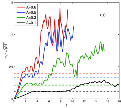
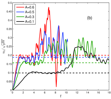
Figure 8: Time variations of the (a) normalized bubble amplitude and (b) normalized bubble velocity in the immiscible RTI with various Atwood numbers. The dashed lines represent the analytical solutions of the classic potential flow model Goncharov .

We also measured the time variations of the spike and bubble normalized velocities with various Atwood numbers and plotted the results in Figs. 8(a) and 8(b). From these figures, the development of the single-mode instability in regardless of the Atwood number can also be divided into four distinguishing stages. In the linear stage, the perturbation develops in the form of an exponential function with the spike growth factor, which shows an increase with the Atwood number. The basic trend that the bubble velocity at the linear stage increases with the Atwood number was also observed, but the relative growth was slowly decreased. For the cases of $A=0.6$ and $A=0.5$, the developments of the bubble velocities are very similar at the linear stage, and the curves are even almost overlapped at the saturated velocity stage. This indicates that when the Atwood number is large enough, it no longer has a significant effect on the bubble velocity at the early stage. In the saturated velocity stage, the spike and bubble show to grow with nearly constant velocities and their values are found to increase with the Atwood number. For comparisons, the asymptotic velocities of the potential flow theory Goncharov depending on the Atwood number are also shown in Figs. 8(a) and 8(b). It can be seen that all the numerical predictions for the spike and bubble saturated velocities agree well with the analytical solutions in general. In addition, we can also find that durations of the saturated velocity stages for both spike and bubble decrease with the increase of the Atwood number and specially the sustaining time for the case of 0.6 is very transient. We can anticipate that the saturated velocity stage for the spike would disappear if continue to enlarge the Atwood number. This is because the vortices are generated faster at a higher Atwood number that accelerates the spike and bubble velocities exceeding than the asymptotic solutions such that the maintenance time of the quasi-steady state becomes shorter. Following the saturated velocity stage, the spike and bubble velocities begin to diverge from the ones obtained from potential flow theory and the growth of the stability enters into the reacceleration stage. The reacceleration stage for the spike emerges at earlier time than that of the bubble, which is more obvious with the increase of the Atwood number. The discrete vortices are first produced in the vicinity of the spike, and there is a certain distance between the generated vortices and the bubble tip, which thus leads to the time lag of the bubble entering the reacceleration stage than the spike. Lastly, the spike and bubble velocities at the chaotic development stage are unstable, presenting a state of some fluctuations with time, while the fluctuant range shows an increase with the Atwood number.

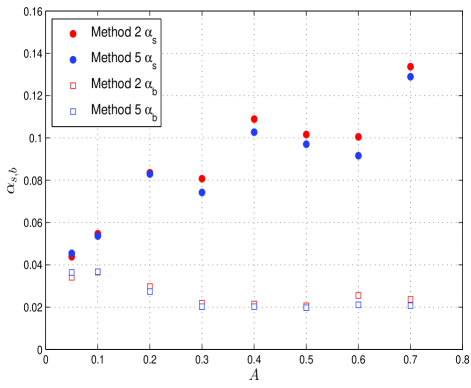
Figure 9: Dependencies of the spike and bubble growth rates $\alpha_{s}$ and $\alpha_{b}$ on the Atwood number.

To reveal the late-time growth law of single-mode instability, we also measured the spike and bubble growth rates under a wide range of Atwood numbers from 0.05 to 0.7, which are the most concerned physical quantities in the study of interfacial instability phenomenon. We used two popular statistic methods to calculate the spike and bubble growth rates with different Atwood numbers and plotted the results in Fig. 9. It can be found that the computed growth rates obtained by the two methods are close to each other. For low Atwood number less than 0.1, the difference between the spike and bubble growth rates is small, which indicates the nearly symmetric developments of the spike and bubble fronts. However, for high Atwood numbers, the spike growth rate is remarkably larger than that of the bubble, implying the growth of the single-mode RTI becomes increasingly asymmetric about the positions of the spike and bubble interfaces. In addition, we can also observe from Fig. 9 that the spike growth rate shows an overall trend of the increase with the Atwood number, while the bubble growth rate has a slightly decrease with the Atwood number at first and then seems to be independence of the Atwood number approaching to a constant of 0.0215. It is worth noting that the predicted curves for spike and bubble growth rates of single-mode RTI are very similar to the ones reported in the experimental studies of the multi-mode phenomenon Akula ; Dimonte ; Banerjee1 .

IV CONCLUSIONS

In this paper, the late-time evolution of the immiscible single-mode RTI is studied by using the phase field lattice Boltzmann method, which mainly includes two aspects: (1) the influence of wide Reynolds numbers on the development of single-mode RTI with a moderate high Atwood number and (2) the influence of different Atwood numbers on the growth of single-mode RTI at a large Reynolds number. Numerical results show that the single-mode instability with a Atwood number of 0.7 presents distinct interfacial dynamics under different Reynolds numbers. For high Reynolds numbers, the phase interfaces roll up at multiple positions caused by the KH instability and eventually formed into a complicated topology structure in addition to numerous visible droplets. As the Reynolds number decreases, the interfaces become more and more smooth and even the roll-up or breakup phenomenon does not occur at extremely small Reynolds numbers. In addition, we summarized the development of the single-mode RTI with high Reynolds numbers into four different stages, including the linear growth, saturated velocity growth, reacceleration and chaotic development stages. The spike and bubble velocities at the saturated velocity stage are quantitatively consistent with the asymptotic solutions of the potential flow model, although the lasting time of the spike’s stage is transient and it is expected that this stage for the spike would disappear by continuously enlarging the Atwood number. The spike and bubble amplitudes at the late-time chaotic stage exhibit quadratic growths characterized by two important parameters of the spike and bubble growth rates. Here we also conducted a comparison of several statistical approaches for computing the growth rate coefficients and two preferential methods are suggested. It is shown that the computed spike and bubble growth rates for a moderately high Atood number of 0.7 approach to 0.13 and 0.022, respectively. As the Reynolds number is reduced, some later stages cannot be reached sequentially. Four different growth stages can be also observed in the single-mode RTI with various Atwood numbers, while the time instants entering these stages are different, which is related to the propagation of vortex in the development process. Moreover, we calculated the growth rates of the spike and bubble under different Atwood numbers. For $A>0.2$, the bubble growth rate is basically maintained at a steady value of 0.0215, indicating that it is independence of the initial density ratio, while the spike coefficient shows an increase with the Atwood number in general. The present investigation only focused on the single-mode RTI between two incompressible fluids and the effect of compressibility on the late-time growth of RTI would be an interested subject Lai ; Luoxs ; Wieland , which constitutes one of our future works.

References

- (1) Y. Zhou, Rayleigh-Taylor and Richtmyer-Meshkov instability induced flow, turbulence, and mixing. I, Phys. Rep. 720-722, 1-136 (2017).
- (2) Y. Zhou, Rayleigh-Taylor and Richtmyer-Meshkov instability induced flow, turbulence, and mixing. II, Phys. Rep. 723-725, 1-160 (2017).
- (3) L. Rayleigh, Investigation of the character of the equilibrium of an incompressible heavy fluid of variable density, Proc. London Math. Soc. 14, 170-177 (1883); G. I. Taylor, The instability of liquid surfaces when accelerated in a direction perpendicular to their plane, Proc. R. Soc. London, Ser. A 201, 192 (1950).
- (4) D. J. Lewis, The instability of liquid surfaces when accelerated in a direction perpendicular to their planes. II, Proc. R. Soc. Lond. A 202, 81-96 (1950).
- (5) R. Bellman and R. H. Pennington, Effects of surface tension and viscosity on Taylor instability, Q. Appl. Math. 12, 151-162 (1954).
- (6) M. Mitchner and R. K. M. Landshoff, Rayleigh-Taylor instability for compressible fluids, Phys. Fluids 7, 862 (1964).
- (7) M. S. Plesset and C. G. Whipple, Viscous effects in Rayleigh-Taylor instability, Phys. Fluids 17, 1-7 (1974).
- (8) R. Menikoff, R. C. Mjolsness, D. H. Sharp, and C. Zemach, Unstable normal mode for Rayleigh-Taylor instability in viscous fluids, Phys. Fluids 20, 2000 (1977).
- (9) D. H. Sharp, An overview of Rayleigh-Taylor instability, Physica D 12, 3 (1984).
- (10) G. Boffetta and A. Mazzino, Incompressible Rayleigh-Taylor turbulence, Annu. Rev. Fluid Mech. 49, 119-143 (2017).
- (11) D. Livescu, Turbulence with large thermal and compositional density variations, Annu. Rev. Fluid Mech. 52 309-341 (2020).
- (12) W. H. Cabot and A. W. Cook, Reynolds number effects on Rayleigh-Taylor instability with possible implications for type Ia supernovae, Nat. Phys. 2, 562-568 (2006).
- (13) R. Adkins, E. M. Shelton, M.-C. Renoult, P. Carles, and C. Rosenblatt, Interface coupling and growth rate measurements in multilayer Rayleigh-Taylor instabilities, Phys. Rev. Fluids 2, 062001(R) (2017).
- (14) K. U. Kobayashi and R. Kurita, Unstable yet static initial state: A universal method for studying Rayleigh-Taylor instability and lock exchange, Phys. Rev. Fluids 4, 013901 (2019)
- (15) G. Dimonte, Dependence of turbulent Rayleigh-Taylor instability on initial perturbations, Phys. Rev. E 69, 056305 (2004).
- (16) D. Layzer, On the instability of superposed fluids in a gravitational field, Astrophys. J. 122, 1-12 (1955).
- (17) U. Alon, J. Hecht, D. Ofer, D. Shvarts, Power laws and similarity of Rayleigh-Taylor and Richtmyer-Meshkov mixing fronts at all density ratios, Phys. Rev. Lett. 74, 534-537 (1995).
- (18) K. O. Mikaelian, Analytic approach to nonlinear Rayleigh-Taylor and Richtmyer-Meshkov instabilities, Phys. Rev. Lett. 80, 508-511 (1998)
- (19) Q. Zhang, Analytical solutions of Layzer-type approach to unstable interfacial fluid mixing, Phys. Rev. Lett. 81 3391-3394 (1998).
- (20) V. N. Goncharov, Analytical model of nonlinear, single-mode, classical Rayleigh-Taylor instability at arbitrary Atwood numbers, Phys. Rev. Lett. 88, 134502 (2002).
- (21) D. Oron, L. Arazi, D. Kartoon, A. Rikanati, U. Alon, and D. Shvarts, Dimensionality dependence of the Rayleigh-Taylor and Richtmyer-Meshkov instability late-time scaling laws, Phys. Plasmas 8, 2883 (2001).
- (22) R. Betti and J. Sanz, Bubble acceleration in the ablative Rayleigh-Taylor instability, Phys. Rev. Lett. 97, 205002 (2006).
- (23) S. I. Sohn, Effects of surface tension and viscosity on the growth rates of Rayleigh-Taylor and Richtmyer-Meshkov instabilities, Phys. Rev. E 80, 055302 (2009).
- (24) R. Banerjee, L. Mandal, S. Roy, M. Khan, and M. R. Guptae, Combined effect of viscosity and vorticity on single mode Rayleigh-Taylor instability bubble growth, Phys. Plasmas 18, 022109 (2011).
- (25) J. T. Waddell, C. E. Niederhaus, and J. W. Jacobs, Experimental study of Rayleigh-Taylor instability: Low Atwood number liquid systems with single-mode initial perturbations, Phys. Fluids 13, 1263-1273 (2001).
- (26) J. Glimm, X. L. Li, and A. D. Lin, Nonuniform approach to terminal velocity for single mode Rayleigh-Taylor instability, Acta Math. Appl. Sin. 18, 1-8 (2002).
- (27) P. Ramaprabhu, G. Dimonte, Y. N. Young, A. C. Calder, B. Fryxell, Limits of the potential flow approach to the single-mode Rayleigh-Taylor problem, Phys. Rev. E 74(6), 066308 (2006).
- (28) J. P. Wilkinson and J. W. Jacobs, Experimental study of the single-mode three-dimensional Rayleigh-Taylor instability, Phys. Fluids 19, 124102 (2007).
- (29) P. Ramaprabhu, G. Dimonte, P. Woodward, C. Fryer, G. Rochefeller, K. Muthuraman, P.-H. Lin, and J. Jayaraj, The late-time dynamics of the single-mode Rayleigh-Taylor instability, Phys. Fluids 24, 074107 (2012)
- (30) T. Wei, and D. Livescu, Late-time quadratic growth in single-mode Rayleigh-Taylor instability, Phys. Rev. E 86, 046405 (2012).
- (31) H. Liang, Q. X. Li, B. C. Shi, and Z. H. Chai, Lattice Boltzmann simulation of three-dimensional Rayleigh-Taylor instability, Phys. Rev. E 93, 033113 (2016).
- (32) X. L. Hu, H. Liang, H. L. Wang, Lattice Boltzmann method simulations of the immiscible Rayleigh-Taylor instability with high Reynolds numbers, Acta Phys. Sin. 69, 044701 (2020).
- (33) Z. X. Hu, Y. S. Zhang, B. L. Tian, Z. W. He, L. Li, Effect of viscosity on two-dimensional single-mode Rayleigh-Taylor instability during and after the reacceleration stage, Phys. Fluids 31, 104108 (2019).
- (34) X. Bian, H. Aluie, D. X. Zhao, H. S. Zhang, D. Livescu, Revisiting the late-time growth of single-mode Rayleigh-Taylor instability and the role of vorticity, Physica D 403, 132250 (2020).
- (35) H. Liang, B. C. Shi, Z. L. Guo, Z. H. Chai, Phase-field-based multiple-relaxation-time lattice Boltzmann model for incompressible multiphase flows, Phys. Rev. E 89, 053320 (2014).
- (36) D. Jacqmin, Calculation of two-phase Navier-Stokes flows using phase-field modeling, J. Comput. Phys. 155, 96-127 (1999).
- (37) J. Shen, J. Xu, J. Yang, A new class of efficient and robust energy stable schemes for gradient flows, SIAM Rev. 61, 474-506 (2019).
- (38) Y. Q. Zu and S. He, Phase-field-based lattice Boltzmann model for incompressible binary fluid systems with density and viscosity contrasts, Phys. Rev. E 87, 043301 (2013).
- (39) H. Liang, J. R. Xu, J. X. Chen, Z. H. Chai, B. C. Shi, Lattice Boltzmann modeling of wall-bounded ternary fluid flows, Appl. Math. Model. 73, 487-513 (2019)
- (40) H. Liang, X. L. Hu, X. F. Huang, and J. R. Xu, Direct numerical simulations of multi-mode immiscible Rayleigh-Taylor instability with high Reynolds numbers, Phys. Fluids 31, 112104 (2019).
- (41) Z. L. Guo and C. Shu, Lattice Boltzmann Method and its Applications in Engineering, World Scientific, Singapore, 2013.
- (42) Y. K. Wei, H. Yang, Z. Lin, Z. D. Wang, and Y. H. Qian, A novel two-dimensional coupled lattice Boltzmann model for thermal incompressible flows, Appl. Math. Comput. 339, 556-567 (2018).
- (43) Z. H. Chai, H. Liang, R. Du, B. C. Shi, A lattice Boltzmann model for two-phase flow in porous media, SIAM J. Sci. Comput. 41, B746-B772 (2019).
- (44) Z. D. Wang, Y. K. Wei, Y. H. Qian, A bounce back-immersed boundary-lattice Boltzmann model for curved boundary, Appl. Math. Model. 81, 428-440 (2020).
- (45) P. Lallemand and L. S. Luo, Theory of the lattice Boltzmann method: dispersion, dissipation, isotropy, Galilean invariance, and stability, Phys. Rev. E 61, 6546-6562 (2000)
- (46) X. Y. He, R. Y. Zhang, S. Y. Chen, G. D. Doolen, On the three-dimensional Rayleigh-Taylor instability, Phys. Fluids 11, 1143-1152 (1999).
- (47) S. I. Abarzhi, A. Gorobets, and K. R. Sreenivasan, Rayleigh-Taylor turbulent mixing of immiscible, miscible and stratified fluids, Phys. Fluids 17, 081705 (2005).
- (48) K. R. Sreenivasan, On the scaling of the turbulence energy dissipation rate, Phys. Fluids 27, 1048 (1984).
- (49) J. R. Ristorcelli, T. T. Clark, Rayleigh-Taylor turbulence: self-similar analysis and direct numerical simulations, J. Fluid Mech. 507, 213-253 (2004).
- (50) A. W. Cook, W. Cabot, and P. L. Miller, The mixing transition in Rayleigh-Taylor instability, J. Fluid Mech. 511, 333-362 (2004).
- (51) T. T. Clark, A numerical study of the statistics of a two-dimensional Rayleigh-Taylor mixing layer, Phys. Fluids 15, 2413-2423 (2003).
- (52) D. H. Olson, J. W. Jacobs, Experimental study of Rayleigh-Taylor instability with a complex initial perturbation, Phys. Fluids 21, 034103 (2009).
- (53) B. Akula, D. Ranjan, Dynamics of buoyancy-driven flows at moderately high Atwood numbers, J. Fluid Mech. 795, 313-355 (2016).
- (54) T. F. Luo, J. C. Wang, C. Y. Xie, M. P. Wan, and S. Y. Chen, Effects of compressibility and Atwood number on the single-mode Rayleigh-Taylor instability, Phys. Fluids 32, 012110 (2020).
- (55) G. Dimonte and M. Schneider, Density ratio dependence of Rayleigh-Taylor mixing for sustained and impulsive acceleration histories, Phys. Fluids 12, 304-321 (2000).
- (56) A. Banerjee, W. N. Kraft and M. J. Andrews, Detailed measurements of a statistically steady Rayleigh-Taylor mixing layer from small to high Atwood numbers, J. Fluid Mech. 659, 127-190 (2010).
- (57) H. L. Lai, A. G. Xu, G. C. Zhang, Y. B. Gan, Y. J. Ying, and S. Succi, Nonequilibrium thermohydrodynamic effects on the Rayleigh-Taylor instability in compressible flows, Phys. Rev. E 94, 023106 (2016).
- (58) X. S. Luo, F. Zhang, J. C. Ding, T. Si, J. M. Yang, Z. G. Zhai, C. Y. Wen, Long term effect of Rayleigh-Taylor stabilization on converging Richtmye-Meshkov instability, J. Fluid Mech. 849, 231-244 (2018).
- (59) S. A. Wieland, P. E. Hamlington, S. J. Reckinger, and D. Livescu, Effects of isothermal stratification strength on vorticity dynamics for single-mode compressible Rayleigh-Taylor instability, Phys. Rev. Fluids 4, 093905 (2019).