Distributed Many-to-Many Protein Sequence Alignment using Sparse Matrices

Abstract

Identifying similar protein sequences is a core step in many computational biology pipelines such as detection of homologous protein sequences, generation of similarity protein graphs for downstream analysis, functional annotation, and gene location. Performance and scalability of protein similarity search have proven to be a bottleneck in many bioinformatics pipelines due to increase in cheap and abundant sequencing data. This work presents a new distributed-memory software PASTIS. PASTIS relies on sparse matrix computations for efficient identification of possibly similar proteins. We use distributed sparse matrices for scalability and show that the sparse matrix infrastructure is a great fit for protein similarity search when coupled with a fully-distributed dictionary of sequences that allow remote sequence requests to be fulfilled. Our algorithm incorporates the unique bias in amino acid sequence substitution in search without altering basic sparse matrix model, and in turn, achieves ideal scaling up to millions of protein sequences.

I Introduction

One of the most fundamental tasks in computational biology is similarity search. Its variants can be used to map short DNA sequences to a reference genome or find homologous regions between nucleotide sequences, such as genes that are the basic functional unit of heredity. A pair of genes is homologous if they both descend from a common ancestor. The DNA sequence of a gene contains the information to build amino acid sequences constituting proteins.

Computing sequence similarity is often used to infer homology because homologous sequences share significant similarities despite mutations that happen since the evolutionary split. While the similarity computation can be carried out in the DNA sequence space, it is more often performed in the amino acid sequence space. This is because the amino acid sequence is less redundant, resulting in fewer false positives. In this paper, we will refer to this problem of inferring homology in the amino acid space as protein homology search.

Protein homology search has numerous applications. For example, functional annotation uses known amino acid sequences to assign functions to unknown proteins. Another example area of application is gene localization, which is crucial to identify genes that may affect a given disease or gain insight about a particular functionality of interest. The primary motivation of our work is the identification of protein families, which are groups of proteins that descend from a common ancestor. It is a hard problem since the relationship between sequence similarity and homology is imprecise, meaning that one cannot use a similarity threshold to accurately conclude that two proteins are homologous or belong to the same family.

Different algorithms attempt to infer homology directly via similarity search [1, 2] with variable degree of success in terms of sensitivity and specificity. Alternatively, one can perform a similarity search within a protein data set and construct a similarity graph [3, 4, 5, 6], and then feed it into a clustering algorithm [7, 8, 9, 10] to ultimately identify protein families. The advantage of the latter approach is that the clustering algorithm can use global information to determine families more accurately. For example, if two proteins $P1$ and $P2$ are incorrectly labeled as homologous by the similarity search, this false positive link can be ignored by the clustering algorithm if it is not supported by the rest of the similarity graph (say if the neighbors of $P1$ and $P2$ are distinct except for $P1$ and $P2$ themselves). Likewise, missed links (false negatives) can be recovered by the clustering algorithm using the topology of the graph. The disadvantage of this approach lies in the computational cost of storing the similarity graph and executing of the subsequent clustering algorithm. Dual-purpose tools such as Many-against-Many sequence searching (MMseqs2) [3] can be used to either directly cluster proteins or to generate a protein similarity graph, depending on their settings.

Recent advancements in shotgun metagenomics, where a metagenome is collected from an environmental sample and it is thus composed of DNA from different species, are leading to the expansion of the known protein space [11]. The massive amount of data associated with modern isolate genome and metagenome databases have rendered many existing tools too slow in constructing protein similarity graphs. Distributed parallel computation is one way to efficiently manipulate this data deluge.

In this paper, we present a fully distributed pipeline called Protein Alignment via Sparse Matrices (PASTIS) for large-scale protein similarity search. PASTIS constructs similarity graphs from large collections of protein sequences, which in turn can be used by a graph clustering algorithm to accurately discover protein families. A major novelty of PASTIS is its use of distributed sparse matrices as its underlying data structure. Not only the sequences and their $k$-mers are stored through sparse matrices, but also the substitute $k$-mers that are critical for controlling sensitivity and specificity during sequence overlapping. We develop custom semirings in sparse matrix computations to enable different types of alignments. PASTIS extensively hides communication and exploits the symmetricity of the similarity matrix to achieve load balance. We present detailed evaluations about parallel performance and relevance. We demonstrate the scalability of PASTIS by scaling it up to 2025 nodes (137,700 cores) and show that its accuracy is on par with MMseqs2.

Our resulting software, PASTIS, is available publicly as open source at https://github.com/PASSIONLab/PASTIS. The rest of this paper is organized as follows. Section II describes the problem we address and Section III presents the related work. In Section IV we describe our methodology for forming the similarity graph and then we focus on its parallel aspects in Section V. We evaluate our approach in Section VI and we conclude in Section VII.

II Background

Protein homology search, as introduced in Section I, is modeled as a sequence similarity searching problem. Herein, we formally define the notation and the problem.

Let $S=\{s_{1},s_{2},\dots,s_{n}\}$ be a set of $n$ protein sequences. Define the Protein Similarity Graph (PSG) graph $G=(V,E)$ as $V=S$ and $E=\{(s_{i},s_{j})~{}|~{}s_{i}$ and $s_{j}$ exceed a given similarity threshold$\}$. The weight of an edge $(s_{i},s_{j})$ is denoted with $w(s_{i},s_{j})$ and it indicates the strength of similarity between sequences $s_{i}$ and $s_{j}$. A k-mer or seed is defined as a subsequence of a given sequence $s$ with fixed length $k$.

The problem we address in this work is defined as follows. Given $p$ processing elements, a set $S$ of proteins, and similarity constraints, compute $G=(V,E)$ efficiently in parallel. Figure 1 depicts the base pipeline to form the similarity graph.

II-A Combinatorial BLAS (CombBLAS)

CombBLAS [12] is a distributed memory parallel graph library that is based on sparse matrix and vector operations on arbitrary user-defined semirings. A semiring consists of two binary operators, addition and multiplication, that satisfy certain requirements. CombBLAS allows users to define their own types for matrix and vector elements and overload the operations on sparse matrices. This allows it to express a broad range of algorithms that operate on graphs.

CombBLAS supports MPI/OpenMP hybrid parallelism and uses a 2D block decomposition for distributed sparse matrices. The 2D decomposition of the matrix constrains most of the communication operations to rows/columns of the process grid and enables better scalability than the 1D decomposition. Among several operations supported by CombBLAS, Sparse General Matrix Multiply (SpGEMM) is heavily utilized by PASTIS and it contains several distinct optimizations. Distributed SpGEMM in CombBLAS uses a scalable 2D Sparse SUMMA [13] algorithm, and for the local multiplication it uses a hybrid hash-table and heap-based algorithm that is faster than the existing libraries [14]. Another distributed matrix library that supports semiring algebra on sparse matrices is the Cyclops Tensor Framework (CTF) [15]. Both CTF and CombBLAS support 2D as well as 3D SpGEMM algorithms.

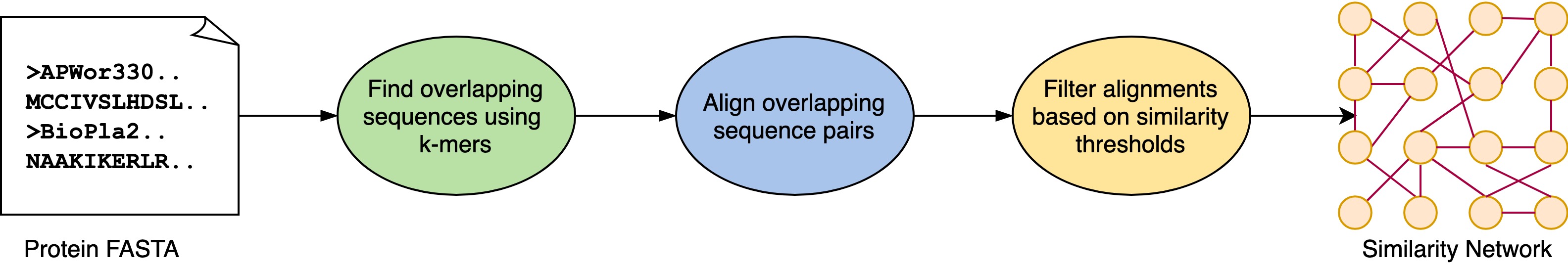
Figure 1: Homology detection pipeline.

III Related Work

pGraph [16] is a distributed software to build protein homology graph. It is similar to PASTIS but with a different distributed implementation and a different way of detecting homologous sequences. Given an input sequence set $S$, it uses a suffix tree based algorithm [17] to identify pairs of sequences that pass a user-defined criteria. These pairs are then aligned using the Smith-Waterman algorithm [18]. pGraph distributed implementation includes a super-master process and a collection of subgroups. Each subgroup consists of a master, a set of producers, and a set of consumers. The producers in each subgroup are responsible for the generation of sequence pairs in parallel, while the consumers perform alignment on those pairs. The master regulates producers and consumers such that no overactive producers exist in the system while at the same time keeping consumers busy. The super-master acts as a regulatory body across all subgroups. One caveat with the producer-consumer approach is that sequence data corresponding to a generated pair may not lie within the local memory of the consumer handling that pair. pGraph introduces two options to overcome this problem: (a) reading from disk or (b) communicating remote sequences from other processes. Both techniques incur latencies, however, their experiments suggest that remote sequence fetching over the network is more efficient than reading from disk. Their results show linear scaling for a set of $\approx 2.5$ million sequences, where a total of $5.3$ billion pairs were aligned.

BELLA is a shared-memory software for overlap detection and alignment for long-read de novo genome assembly and error correction [19], where long-read indicates a category of sequencing data. Despite different objectives, BELLA is the first work to formulate the overlap detection problem as a SpGEMM. It uses a seed-based approach to detect overlaps and uses a sparse matrix, $\mathbf{A}$, to represent its data, where the rows represent nucleotide sequences and columns represent $k$-mers. $\mathbf{A}$ is then multiplied by $\mathbf{A}^{\mbox{\scriptsize\sf T}}$, yielding a sparse overlap matrix $\mathbf{A}\mathbf{A}^{\mbox{\scriptsize\sf T}}$ of dimensions $S$-by-$S$, where each non-zero cell $(i,j)$ of the overlap matrix stores the number of common $k$-mers between the $i$th and $j$th sequences, and their positions in the corresponding sequence pair. In this work, we adopt this technique and extend it to implement a distributed memory k-mer matching. BELLA also has a distributed version, diBELLA [20], that is being developed. However, it operates on nucleotide sequences and computes overlap detection using distributed hash tables rather than distributed SpGEMM.

MMseqs2 [3] is a software to find target sequences similar to a given query sequence by searching a precomputed index of target sequences. A target sequence is chosen to be aligned against the query only if they share two similar k-mers along the same diagonal. The notion of similar k-mers is comparable to the substitute k-mers of our work (Section IV-C). The authors claim the two-k-mer approach increases the sensitivity lowering the probability of that match happening by chance. Notably, a pair could have more than one diagonal containing two similar k-mers. Once a pair is chosen, an ungapped alignment is performed on the k-mers on each diagonal. Additionally, a gapped alignment is performed if the diagonal with the best ungapped score passes a given threshold. MMseqs2 is a faster and more sensitive search tool compared to its popular counterpart Basic Local Alignment Search Tool (BLAST) and it can run in parallel on distributed memory systems.

LAST [5] is another heuristics-based sequence search tool. LAST also uses matching subsequences to identifying similar sequences but it supports a richer notion of seed than the regular k-mer one. LAST provides both spaced seeds and substitute seeds. A spaced seed can be thought of as supporting the wildcard ‘*’ in the seed definition, so that certain positions of a k-mer could be ignored or matched regardless of the character (or amino acid) in the target sequence at that position. A substitute seed modifies this idea by restricting the wildcard matching to a group of designated characters at each position. Besides introducing extended seed patterns, LAST takes a step further allowing adaptive seed length. This features allows LAST to increase the match sensitivity by repeatedly matching a seed pattern until the number of matches in the target sequence matches or drops below a frequency threshold [5]. Currently, LAST implementation is based on suffix array and runs in a single compute node with optional shared memory parallelism. Despite the sensitivity advantages, the shared memory parallelism is a bottleneck for large data sets as its runtime is in the order of days.

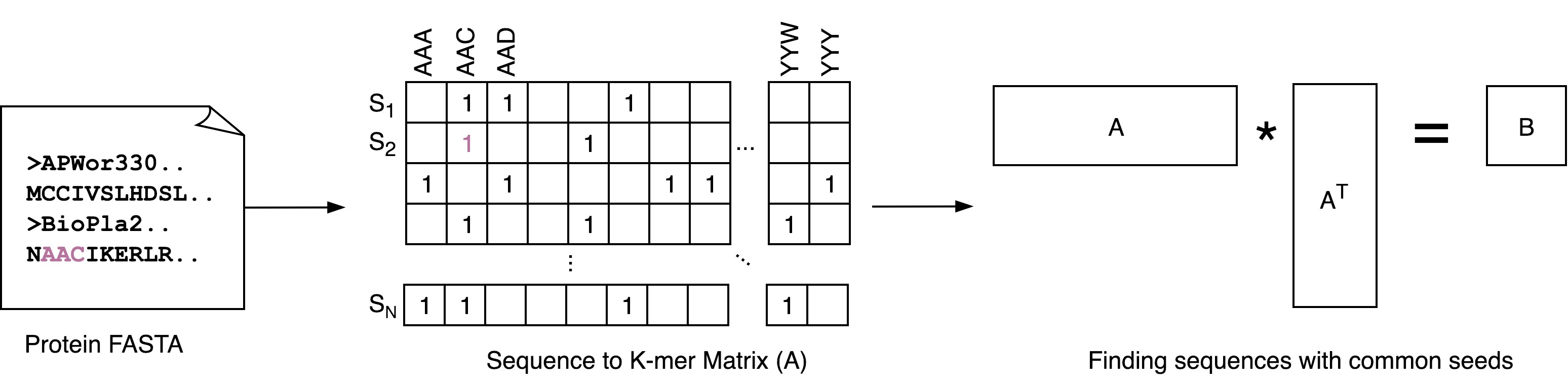
Figure 2: Overlap detection in PASTIS.

Double Index Alignment of Next-generation Sequencing Data (DIAMOND) [6] utilizes a double indexing approach which determines the list of all seeds in both reference and query sequences. The double indexing strategy is cache-friendly as it increases the data locality. To attain high sensitivity, DIAMOND utilizes spaced seeds of certain weight and shape. Different shape and weight combinations can be used to achieve different levels of sensitivity. Another important feature of DIAMOND is that it uses a reduced amino acid alphabet for greater sensitivity. This also makes DIAMOND more memory-efficient as it results in smaller index sizes.

IV PASTIS Concepts

The PSG, $G=(V,E)$, can technically be a clique, where an alignment algorithm would perform $O(n^{2})$ comparisons and find some similarity between each pair of sequences. Nevertheless, only pairs above a certain similarity threshold are assumed to be biologically related via a common ancestor. This enables PASTIS to avoid the expensive $O(n^{2})$ alignments and exploit efficient sparse matrix operations in constructing the PSG. PASTIS adheres to the pipeline shown in Figure 1 to compute the PSG. Other heuristics-based sequence alignment tools, described in Section III, also follow similar stages. In the following sections, we describe how these stages are handled in PASTIS.

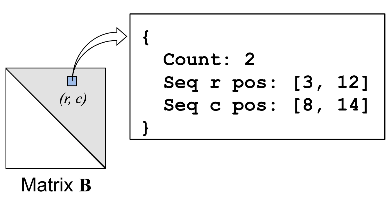
Figure 3: The structure of matrix $\mathbf{B}$ in PASTIS.

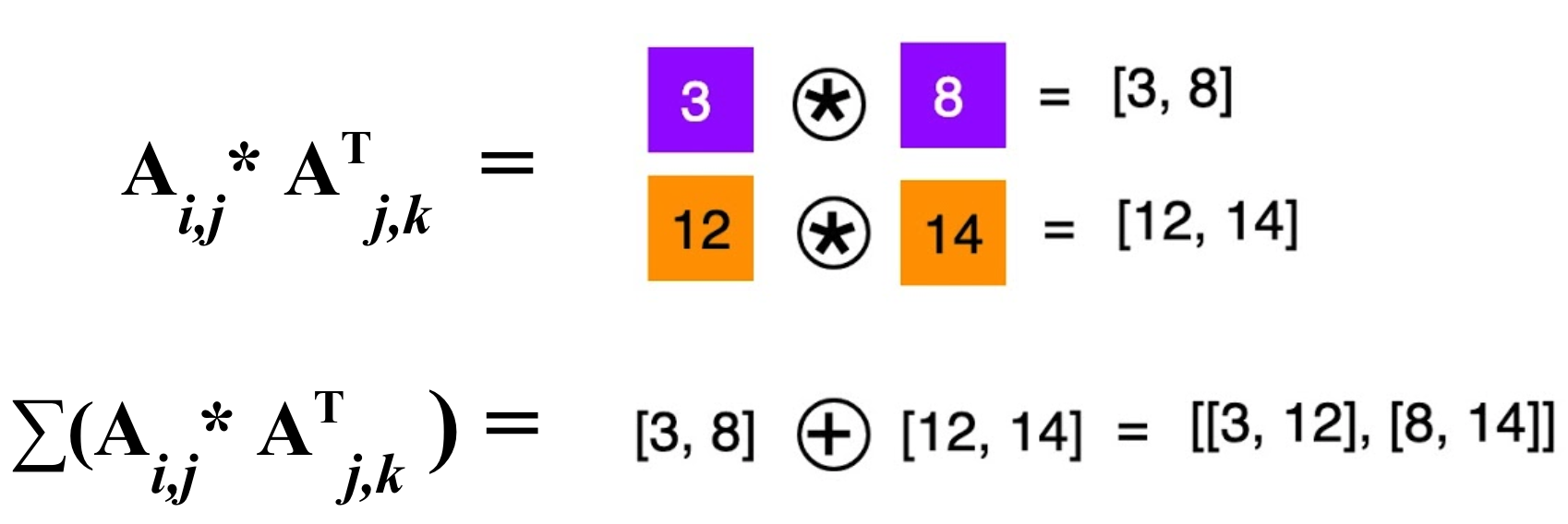
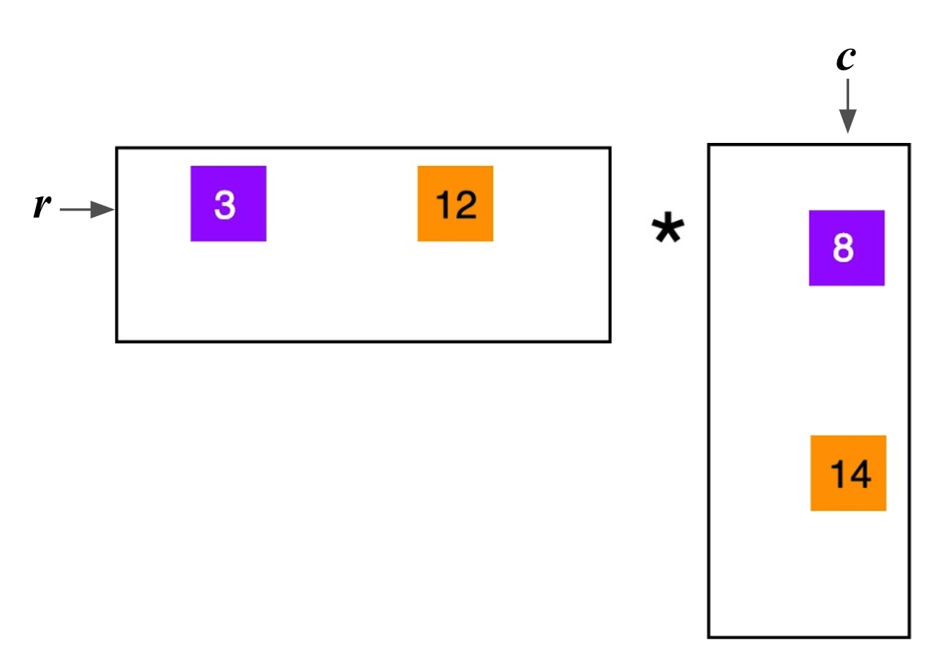
Figure 4: Semiring for exact k-mer matching.

IV-A Overlapping Sequences

PASTIS uses the presence of common k-mers as a heuristic metric, which is a common technique that is also adopted in tools such as BLAST [21], LAST [5], and MMseqs2 [3]. One approach to find these common $k$-mers is to create an index, such as a suffix array, of the input target sequence set and query the same sequence against it. A distributed implementation of this method would require a parallel implementation of the suffix array. Alternatively, we use a sparse matrix based implementation that is highly parallel using existing libraries such as CombBLAS [12].

Figure 2 shows the creation of the $\lvert\textit{sequences}\rvert$-by-$\lvert\textit{{k}-mer}{s}\rvert$ matrix $\mathbf{A}$. A nonzero entry $\mathbf{A}_{ij}$ denotes the existence of k-mer $j$ in sequence $i$. The alphabet determines the number of all possible k-mers. For proteins, there are a total of 24 amino acid bases making the size of the k-mer space $24^{k}$. Once this matrix is constructed, we compute $\mathbf{B}=\mathbf{A}\mathbf{A}^{\mbox{\scriptsize\sf T}}$ of size $n\times n$. If each nonzero entry in $\mathbf{A}$ was marked as $1$ then $\mathbf{B}_{ij}$ would perform exact k-mer matching and be equal to the count of common k-mers between sequences $i$ and $j$. Consequently, we proceed to align sequence pairs $(i,j)$ where $\mathbf{B}_{ij}\neq 0$.

Using SpGEMM to find sequences that share at least one k-mer has been originally proposed in BELLA [19] in the context of overlapping of long error-prone sequences. Importantly, BELLA work did not use distributed data structures nor did it use the substitute k-mers concept we discuss in the next section.

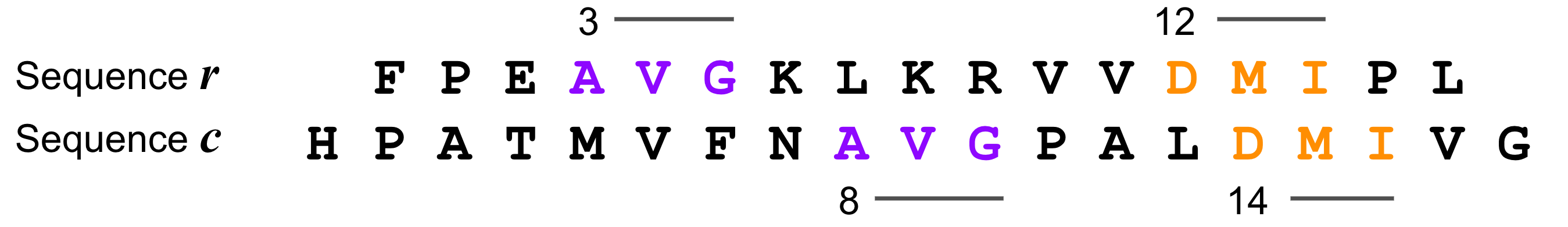
Figure 5: Common k-mers of two sequences.

PASTIS stores the positions of the shared k-mers in each sequence along with the k-mer count as such information is useful in the alignment step. For example, Figure 5 shows the location of two common k-mers, $\mathtt{AVG}$ and $\mathtt{DMI}$, on a pair of sequences $r$ and $c$. Figure 3 shows how this information is recorded in $\mathbf{B}_{rc}$. Notably, $\mathbf{B}$ is symmetric. Therefore, we process only nonzeros belonging to strictly lower or upper triangular portion of it.

In order to yield the custom structure in $\mathbf{B}$ as shown above, we employ a custom semiring to overload the addition and multiplication operators in $\mathbf{A}\mathbf{A}^{\mbox{\scriptsize\sf T}}$. In addition, $\mathbf{A}_{ij}$ represents the starting position of k-mer $j$ in sequence $i$ instead of $1$ for its presence. Figure 4 shows the matrix multiplication with a custom semiring in PASTIS when exact k-mer matching is used. In PASTIS, the multiplication operator saves the position on the two sequences for k-mer $j$ into a pair while the addition operation organizes the seed positions on sequence $r$ into one list and positions of $c$ into another list. Currently, a maximum of two shared k-mer locations per sequence pair are kept out of all such possible pairs. While k-mers attempt to capture the latent features of protein sequences, there is no accepted standard as to which k-mers yield better results than others. In future, we plan to study the effect of different number of k-mers as well as the distance between k-mers.

IV-B Substitute K-mers

$\mathbf{A}\mathbf{A}^{\mbox{\scriptsize\sf T}}$ results in exact k-mer matches. However, our experiments suggest that exact matches pose an excessively strict constraint on the overlapping landscape yielding to significantly low recall. In this context, recall is defined as the ratio between sequence pairs belonging to the same family in both PASTIS output and the original data. Herein, we introduce the notion of substitute k-mers as an approach to improve the recall of this step (see Section VI-B for results about accuracy). Importantly, this is different from the notion of substitute seeds used in LAST [5], which is about specifying a seed as a pattern similar to a regular expression. The similar k-mers concept of MMseqs2 is closest to our approach with the difference being MMseqs2 limiting similar k-mer sets through a scoring threshold whereas PASTIS defines a fixed-sized neighborhood.

In the state-of-the-art, scoring matrices such as BLOSUM62 [22] are used to quantify the chance of a certain amino acid being substituted by another during evolution. While these scores are typically used during the alignment phase, we adopt the notion of “evolution” for k-mers by producing a set of substitute k-mers for any given k-mer. Given a set of substitute k-mers, the algorithm chooses the one with the highest chance to appear in-place of the original k-mer.

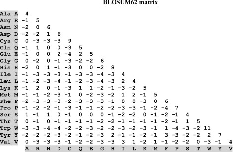
Figure 6: The BLOSUM62 scoring matrix for proteins.

For example, under BLOSUM62 the $\mathrm{3}$-mer $\mathtt{AAC}$ will have a score of $4+4+9=17$ for an exact match. As seen in Figure 6, the base $A$ can be substituted with $S$ for the least amount of penalty. Thus, $\mathrm{3}$-mers $\mathtt{SAC}$ and $\mathtt{ASC}$ both have a score of $1+4+9=14$ when matched with $\mathtt{AAC}$. Continuing with this idea, the next $\mathrm{3}$-mer closest to $\mathtt{AAC}$ is $\mathtt{SSC}$, which has a match score of $1+1+9=11$. In PASTIS, we restrict ourselves to computing $m$ “nearest” such substitute k-mers for any original k-mer present in a sequence.

We remark that $m$-nearest k-mers are not restricted to single substitutions. Depending on the scoring matrix and the values of $m$ and $k$, the $m$-nearest neighbors of a given k-mer include k-mers can be multiple hops away in terms of the edit distance. This can be true even when $m$ is significantly smaller than $k(\lvert\Sigma\rvert-1)$ where $\Sigma$ is the alphabet. If we consider our original example $\mathtt{AAC}$, Figure 6 shows that substitutions in $\mathtt{C}$ cost more than substitutions in $\mathtt{A}$ under BLOSUM62. Given that a match in $\mathtt{C}$ provides a gain of $9$ in the score, even the least costly substitution lowers the score (e.g., to $\mathtt{M}$ whose score is $-1$) by $10$. By contrast, a match in $\mathtt{A}$ only has a score of $4$. Substituting it with $\mathtt{C}$, $\mathtt{D}$, or $\mathtt{T}$, all of which have scores $0$, would only lower the cost by $4$. Therefore, $3$-mers of the form $\{T|C|G\}\{T|C|G\}C$ are all closer to $\mathtt{AAC}$ (at a “distance” of 8) than any $3$-mer of the form $\mathtt{AA*}$ (except $\mathtt{AAC}$ itself), despite requiring two letter substitutions.

Algorithm 1 Find the nearest $m$ substitute k-mers of a given k-mer $r$, using sorted expense matrix $\mathbf{E}$.

1:procedure FindSubKMers($r,\mathbf{E},m$)

2:    $\mathop{\mathit{nbrs}}\nolimits\leftarrow\{\}$ $\triangleright$ neighbor list

3:    $\mathop{\mathit{minmaxheap}}\nolimits\leftarrow\{\}$

4:    $\textsc{Explore}(r,\mathop{\mathit{minmaxheap}}\nolimits,r,\mathbf{E},m)$

5:    while $\lvert\mathop{\mathit{nbrs}}\nolimits\rvert<m$ do

6:         $\mathop{\mathit{mink}}\nolimits\leftarrow\textsc{FindMin}(\mathop{\mathit{minmaxheap}}\nolimits)$

7:         $\mathop{\mathit{nbrs}}\nolimits\leftarrow\mathop{\mathit{nbrs}}\nolimits\cup\mathop{\mathit{mink}}\nolimits$

8:         $\textsc{Explore}(\mathop{\mathit{mink}}\nolimits,\mathop{\mathit{minmaxheap}}\nolimits,r,\mathbf{E},m)$

9:         $\textsc{ExtractMin}(\mathop{\mathit{minmaxheap}}\nolimits)$

10:    end while

11:    return $\mathop{\mathit{nbrs}}\nolimits$

12:end procedure

Given non-uniform scores, the efficient generation of $m$-nearest k-mers is non-trivial. For each k-mer in the data set, we first generate its 1-hop neighbors (i.e., single-substitution k-mers) that are the $m$ nearest. This can be done significantly faster than the naive $O(k(\lvert\Sigma\rvert-1))$ approach if $m$ is small. For each letter in $\Sigma$, we can pre-compute the lowest cost substitutions by simply sorting (in decreasing values) the off-diagonal entries in the corresponding column (or row because the scoring matrix is symmetric) of the scoring matrix. This pre-computation only needs to be done once per scoring matrix rather than for each k-mer, therefore the cost is minuscule. Assuming $m<k(\lvert\Sigma\rvert-1)$, we now just need to simply merge these sorted lists into a single sorted list of length $m$. The crux is that we do not need to touch the entire set of columns during this merging because we only need the top $m$ elements of the final merged list. Hence, the cost of initial list generation is $O(m)$. This initial list is solely composed of single-substitution k-mers and no other single-substitution $k$-mer can be closer to our seed k-mer.

From here, we run an algorithm in the spirit of Dijkstra’s shortest path algorithm. The differences are that (1) we are only interested in paths that are up to length $m$, (2) the edges in our case are implicit (i.e., never materialized) and only generated as needed, and (3) this implicit graph is acyclic; in fact, we are exploring a tree with a branching factor of $(\lvert\Sigma\rvert-1)$. Properties (1) and (3) allow us to stop exploring substitutions in a given position once we know that the current distance is farther than the current $m$-nearest neighbors list. Those positions are marked as inactive. This current $m$-nearest neighbors list is implemented using a max heap (priority queue). For each active position, we iterate over substitutions in increasing distance, using the sorted columns of our scoring matrix. If a substitution gives a score lower than the top of our heap, we push it to our heap. Note that checking the top of the heap with FindMin is $O(1)$ whereas insertion and extraction are $O(\log(m))$, hence it only costs when we find a new $m$-nearest neighbor. If a substitution does not give a score lower than the top of our heap, we mark that position as inactive and not explore any further substitutions. This is possible because we are exploring substitutions in increasing cost, and thus no other substitution on that position can make it to the $m$-nearest neighbor list. The algorithm stops when all of the $k$ k-mer positions are marked as inactive.

The pseudocode to find the most possible substitute k-mers is described in Algorithm 1. Here, the scoring matrix whose row entries are sorted is denoted by $\mathbf{E}$ because it encodes the “expense” we incur in order to substitute the amino acid bases in those k-mers. If the substitution matrix is denoted by $\mathbf{C}$, then $\mathbf{E}=\textnormal{Sort}(\textnormal{Diag}(\mathbf{C})-\mathbf{C})$, where the function Diag() simply creates a diagonal matrix out of its parameter by deleting its off-diagonal entries, and Sort() sorts the rows of a matrix in ascending order.

$\mathbf{E}$ stores both the integer expenses and the bases corresponding to that expense in its auxiliary field, which is accessed by accessible via .base. For example, the first row of $\mathbf{E}$ would be: $\mathbf{E}[1]=\{(0,\mathtt{A}),(3,\mathtt{S}),(4,\mathtt{C}),(4,\mathtt{G}),\ldots\}$ for the BLOSUM62 shown in Figure 6. The first entry of each row is somewhat uninteresting and $\mathbf{E}[i][1]$ (the arrays are 0-indexed) would give the cheapest substitution to the $i$th base. Each individual base in k-mers can be accessed and modified using operator[]. Furthermore, each k-mer object has a list of “free” indices, which are locations that have not been previously substituted by the algorithm. At the beginning, the entire list of indices $[0,k-1]$ is free.

Algorithm 2 Explore the next nearest k-mers of a given k-mer $p$, with respect to a root k-mer $r$ and an existing set of nearest k-mers. The min-max heap $\mathop{\mathit{mmheap}}\nolimits$ is of size $m$.

1:procedure Explore($p,\mathop{\mathit{mmheap}}\nolimits,r,\mathbf{E},m$)

2:    $\mathop{\mathit{minheap}}\nolimits\leftarrow\{\}$ $\triangleright$ stores triplets, sorted by first value

3:    for $idx\in\{\textsc{FreeIdxs}(p)\}$ do $\triangleright$ Free indices of $p$

4:         $\mathop{\mathit{cheap}}\nolimits\leftarrow\mathbf{E}[idx][1]$ $\triangleright$ Cheapest substitution

5:         $\mathop{\mathit{newtuple}}\nolimits\leftarrow(\mathop{\mathit{cheap}}\nolimits+\textsc{Dist}(p,r),\mathop{\mathit{idx}}\nolimits,1)$

6:         $\textsc{Push}(\mathop{\mathit{newtuple}}\nolimits,\mathop{\mathit{minheap}}\nolimits)$

7:    end for

8:    $(\mathop{\mathit{msb}}\nolimits,\mathop{\mathit{fid}}\nolimits,\mathop{\mathit{sid}}\nolimits)\leftarrow\textsc{FindMin}(\mathop{\mathit{minheap}}\nolimits)$

9:    $\triangleright$ $\mathop{\mathit{msb}}\nolimits$ is the minimum substitution cost, $\mathop{\mathit{fid}}\nolimits$ the free index, $\mathop{\mathit{sid}}\nolimits$ the substitution index

10:    if !$\textsc{IsFull}(\mathop{\mathit{mmheap}}\nolimits)$ then $\triangleright$ $\lvert\mathop{\mathit{mmheap}}\nolimits\rvert<m$

11:         repeat

12:             $\textsc{MakeNewSubK}(p,\mathop{\mathit{minheap}}\nolimits,\mathop{\mathit{mmheap}}\nolimits,\mathbf{E})$

13:             $(\mathop{\mathit{msb}}\nolimits,\mathop{\mathit{fid}}\nolimits,\mathop{\mathit{sid}}\nolimits)\leftarrow\textsc{FindMin}(\mathop{\mathit{minheap}}\nolimits)$

14:         until $\textsc{IsFull}(\mathop{\mathit{mmheap}}\nolimits)$

15:    else

16:         $\mathop{\mathit{max}}\nolimits\leftarrow\textsc{FindMax}(\mathop{\mathit{mmheap}}\nolimits)$

17:         while $\mathop{\mathit{msb}}\nolimits<\textsc{Dist}(\mathop{\mathit{max}}\nolimits,r)$ do

18:             $\textsc{MakeNewSubK}(p,\mathop{\mathit{minheap}}\nolimits,\mathop{\mathit{mmheap}}\nolimits,\mathbf{E})$

19:             $(\mathop{\mathit{msb}}\nolimits,\mathop{\mathit{fid}}\nolimits,\mathop{\mathit{sid}}\nolimits)\leftarrow\textsc{FindMin}(\mathop{\mathit{minheap}}\nolimits)$

20:             $\mathop{\mathit{max}}\nolimits\leftarrow\textsc{FindMax}(\mathop{\mathit{mmheap}}\nolimits)$

21:         end while

22:    end if

23:end procedure

IV-C Overlapping with Substitute K-mers

The matrix formulation we used in Section IV-A can be elegantly extended to find overlaps with substitute k-mers. The naive approach is to modify matrix $\mathbf{A}$ with all the substitute k-mers. However, this would be costly. A protein of length $L$ has $L-k+1$ $k$-mers in it. Given that $L$ is often around $100-1000$, this itself is not a problem. However, modifying $\mathbf{A}$ to include all substitute $k$-mer would increase the number of nonzeros in each row to potentially $m\times(L-k+1)$, severely increasing the computational cost and memory consumption.

Instead, we use a second matrix that encodes the k-mer-to-substitute-k-mer mappings. This matrix $\mathbf{S}$ is at most of dimensions $\lvert\Sigma\rvert^{k}\times\lvert\Sigma\rvert^{k}$ but its sparsity is controlled at $m$ nonzeros per row. The matrix $\mathbf{S}$ does not need to be binary, and we can encode substitution costs in it. With this modification, our overlapping computation becomes $\mathbf{A}\mathbf{S}\mathbf{A}^{\mbox{\scriptsize\sf T}}$. Importantly, this requires a new semiring for $\mathbf{A}\mathbf{S}$ and a slight change to the existing semiring for $(\mathbf{A}\mathbf{S})\mathbf{A}^{\mbox{\scriptsize\sf T}}$. This new semiring chooses the closest k-mer for a substitute k-mer when there is more than one k-mer in a given read that has the same substitute k-mer. For example, suppose a given sequence $i$ has k-mers $k_{p}$ and $k_{q}$ at $\mathbf{A}_{ip}$ and $\mathbf{A}_{iq}$. Also, assume a substitute k-mer $k_{s}$ is common to both $k_{p}$ and $k_{q}$ in $\mathbf{S}$ but each with distances $d_{ps}$ and $d_{qs}$. Even though substitute k-mers do not actually appear in a given sequence, we record the starting position of their closest k-mer as their location. That is, if $d_{ps}\leq d_{qs}$ we would store the position of $k_{p}$ as the starting position of $k_{s}$ and vice versa. We omit the technical details for brevity.

IV-D Sparse Matrix Storage

CombBLAS supports the doubly compressed sparse column (DCSC) format [23] (among others) for storing sparse matrices locally on each process. DCSC is designed for the representation of hypersparse matrices, in which the number of nonzeros is smaller than the number of rows or columns. It is an efficient format for hypersparse matrices in terms of space as it avoids storing pointers of empty columns.

Algorithm 3 Create and insert a new substitute k-mer to an existing set of nearest k-mers, only modifying the free index $\mathop{\mathit{fid}}\nolimits$.

1:procedure MakeNewSubK($p,\mathop{\mathit{minheap}}\nolimits,\mathop{\mathit{mmheap}}\nolimits,r,\mathbf{E}$)

2:    $(\mathop{\mathit{msb}}\nolimits,\mathop{\mathit{fid}}\nolimits,\mathop{\mathit{sid}}\nolimits)\leftarrow\textsc{ExtractMin}(\mathop{\mathit{minheap}}\nolimits)$

3:    $\mathop{\mathit{subk}}\nolimits\leftarrow p$ $\triangleright$ initialize substitute $k$-mer

4:    $\mathop{\mathit{bid}}\nolimits\leftarrow\textsc{IndexOf}(\mathop{\mathit{subk}}\nolimits[\mathop{\mathit{fid}}\nolimits])$ $\triangleright$ Base to index

5:    $\mathop{\mathit{subk}}\nolimits[\mathop{\mathit{fid}}\nolimits]=\mathbf{E}[\mathop{\mathit{bid}}\nolimits][\mathop{\mathit{sid}}\nolimits]\mathtt{.base}$ $\triangleright$ Replace that base

6:    $\textsc{DeleteFreeIdx}(\mathop{\mathit{fid}}\nolimits,\mathop{\mathit{subk}}\nolimits)$

7:    if $\textsc{IsFull}(\mathop{\mathit{mmheap}}\nolimits)$ then

8:         $\textsc{ExtractMax}(\mathop{\mathit{mmheap}}\nolimits)$

9:    end if

10:    $\textsc{Push}(\mathop{\mathit{subk}}\nolimits,\mathop{\mathit{mmheap}}\nolimits)$

11:    $\mathop{\mathit{sid}}\nolimits\leftarrow\mathop{\mathit{sid}}\nolimits+1$ $\triangleright$ Get next cheapest substitution

12:    $\mathop{\mathit{newtuple}}\nolimits\leftarrow(\mathbf{E}[\mathop{\mathit{fid}}\nolimits][\mathop{\mathit{sid}}\nolimits]+\textsc{Dist}(p,r),\mathop{\mathit{fid}}\nolimits,\mathop{\mathit{sid}}\nolimits)$

13:    $\textsc{Push}(\mathop{\mathit{newtuple}}\nolimits,\mathop{\mathit{minheap}}\nolimits)$

14:end procedure

The size of the k-mer space in PASTIS is $\lvert\Sigma\rvert^{k}$, where $\lvert\Sigma\rvert=24$. Even for a relatively small $k$, this results in a large column count in $\mathbf{A}$ and row/column counts in $\mathbf{S}$. Moreover, as these matrices are distributed by CombBLAS among processes in a 2D manner (Section V-A), the columns of submatrices stored in each process become increasingly empty as the process count increases. For example, for the Metaclust50-1M dataset we use in our experiments (which contains 1 million sequences) and for a k-mer size of 6, $\mathbf{A}$ is a 1M $\times$ 244M matrix containing 108M nonzeros, and $\mathbf{S}$ is a 244M $\times$ 244M matrix containing 611M nonzeros. These matrices respectively contain 0.44 and 2.50 nonzeros per column, and when they are distributed among multiple processes, the number of nonzeros per column gets even smaller in the submatrices stored. Hence, to scale to thousands of processes, PASTIS stores submatrices in the DCSC format.

IV-E Alignment of Overlapping Sequences

PASTIS supports two alignment modes for sequence pairs detected in the first step: seed-and-extend with x-drop (XD) [4] and Smith-Waterman (SW) alignment [18].

In XD, PASTIS initiates the alignment starting from the position of the shared k-mers and extending it in both directions until the end of the sequences using gapped x-drop. Since we store up to two shared k-mers, the alignment is performed starting from of both of them separately. The alignment with the best score and that passes the similarity thresholds is retained.

The SW alignment computes a local alignment starting from the beginning of each sequence. Even though the alignment computations initiates at the beginning of the sequences and it is performed until the end, only the local alignment with higher score between the two sequences is returned. In SW, scores cannot assume negative values. In this case, our seed position is ignored and the seed is merely used to mark the two sequences as potentially related and worth aligning. One advantage of this method over seed-and-extend is that alignment quality does not depend on the seeds we found. The implementation of XD and SW is offloaded to the The Library for Sequence Analysis (SeqAn) C++ library [24].

IV-F Sequence Similarity Filter

The last stage of the pipeline is the alignment post-processing, which includes filtering out sequence pairs that fall below certain quality metrics provided to PASTIS. From our experience, these metrics typically include vetoing pairs with alignment similarity less than 30% and length coverage less than 70%.

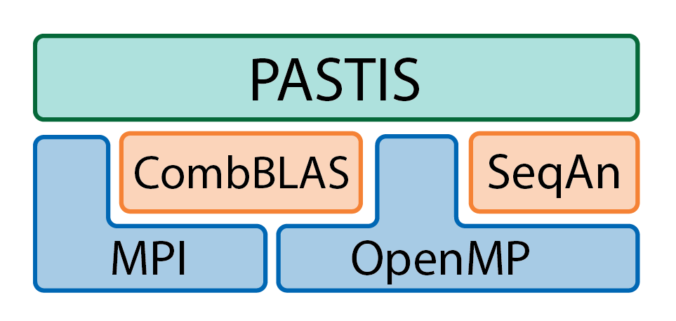
Figure 7: PASTIS software stack. PASTIS implicitly uses MPI and/or OpenMP through CombBLAS and SeqAn libraries. It also explicitly uses both parallel programming paradigms in certain stages.

V PASTIS Distributed Implementation

PASTIS provides a single scalable distributed implementation of the pipeline illustrated in Figure 1. The connections found in the PSG are oblivious to the number of processes used to parallelize PASTIS. This is an important aspect of our tool as it allows reproducible results under different configurations. Some of the suffix array based existing tools such as LAST, in contrast, may produce configuration specific results depending on the physical resource limitations.

The current implementation of PASTIS uses Message Passing Interface (MPI) as its underlying parallel communication library. We assume PASTIS is run with $p=q^{2}$ number of parallel processes, where $q$ is a positive integer. The requirement to have a square number of processes is due to 2D domain decomposition that happens during sparse matrix creation and multiplication using the CombBLAS library. The following sections describe the implementation details along with some of the computation and communication optimizations. Figure 7 shows the libraries and parallel programming paradigms PASTIS relies on.

Among the two libraries utilized by PASTIS, CombBLAS supports hybrid MPI/OpenMP parallelism while SeqAn supports shared-memory parallelism with OpenMP. By utilizing these libraries, PASTIS implicitly makes use of the inherent parallelism in them. Apart from those, PASTIS explicitly makes use of MPI/OpenMP hybrid parallelism as well. For an example, in the preparation of batches of pairwise alignments for SeqAn, it uses OpenMP threads. Then, when SeqAn completes these alignments, the threads at each process again process the output information in parallel to gather necessary statistics for forming the similarity graph. In this way, OpenMP is used both implicitly and explicitly in PASTIS.

V-A Data Partitioning

The input to PASTIS is a set of protein sequences in FAST-All (FASTA) format. We use parallel file I/O to read independent chunks of this file. Each process gets the size of the file and then divides this size evenly by the number of processes. This gives a begin and end location, a chunk, to be read by each process in parallel. It is common that a file chunk read with such splitting may not start and end at sequence margins, so we read a user defined extra amount of bytes in each process. With this approach, each process will ignore any partial sequences at the start of its chunk and read until the end of the last sequence in chunk with possibly reading over on the extra bytes at the end.

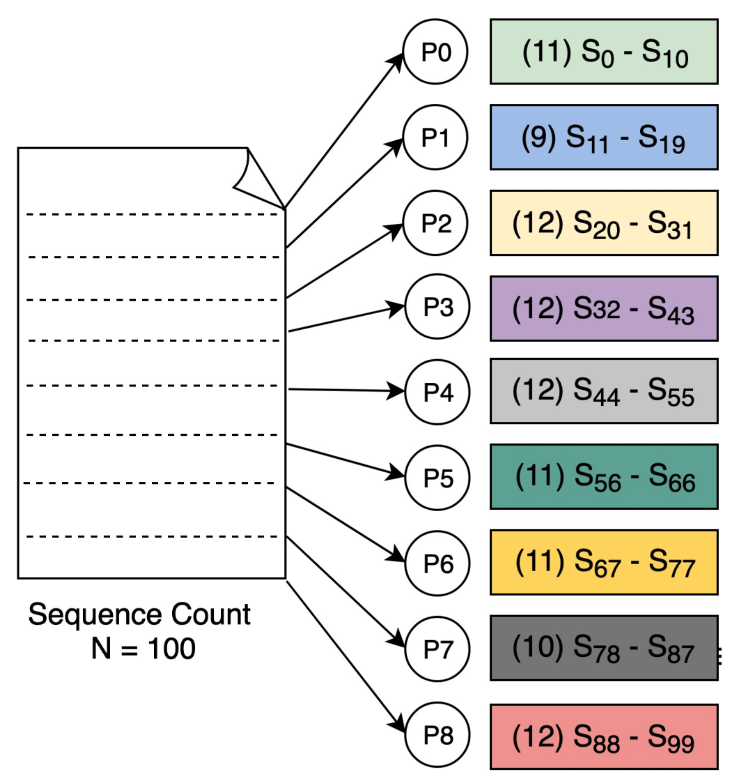
Figure 8: Input sequence partitioning in PASTIS

Figure 8 shows an example of how PASTIS would partition $\mathrm{100}$ sequences among $\mathrm{9}$ processes. Note how some processes have different number of sequences due to the length variation among proteins. This variation does not cause any load imbalance because the runtime of the parallel I/O section depends on the total length of the sequences that is being read and parsed, which is exactly what our implementation balances by choosing process boundaries via assigning each process an equal number of bytes as opposed to an equal number of sequences. The processes then start communicating sequences to fit into a 2D distribution (Section V-C). Each process is responsible for a predefined range of protein IDs in this 2D grid, ensuring load balance by construction.

Internally, PASTIS stores a pointer to the character buffer of its sequences in each process for efficient storage without converting to a separate data structure. It records sequence identifier and data start offsets, so any sequence can be accessed using a local or global index. A parallel prefix sum of sequence counts are computed cooperatively by all processes, so that each process is aware what sequences are stored by which processes.

V-B Seed Discovery

As explained in Section IV-A, seed discovery requires the creation and multiplication of $\mathbf{A}$ with its transpose. The columns $\mathbf{A}$ present a direct mapping to k-mers. Therefore, we compute a unique number for each k-mer as follows.

We index each base in the protein alphabet uniquely from $\mathrm{0}$ to $\mathrm{23}$. Then each base gets a number as $b24^{i}$, where $b$ is the index of the base in the alphabet and $i$ is the zero-based position of the base in the k-mer from right to left. For example, under the $\mathtt{ARNDCQEGHILKMFPSTWYVBZX*}$ alphabet, the $\mathrm{3}$-mer $\mathtt{RCQ}$ will be assigned the id $\mathrm{1\cdot 24^{2}+4\cdot 24^{1}+5\cdot 24^{0}=677}$. Importantly, we only perform this for k-mers present in sequences and not the entire k-mer space.

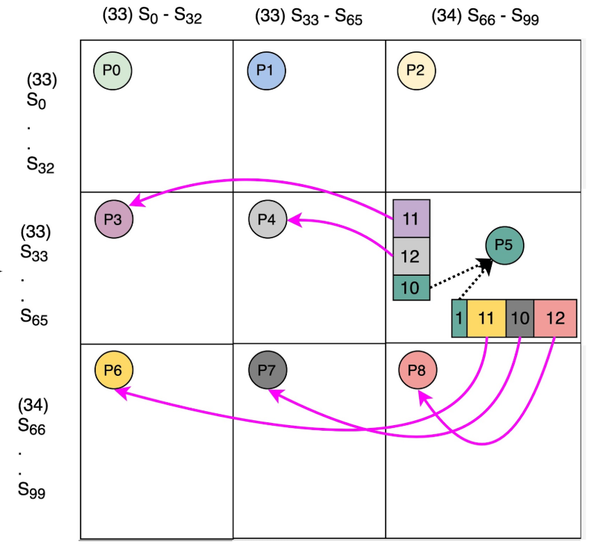
Figure 9: Remote sequence requests from $\mathrm{P5}$ to other processes.

V-C Overlapping Communication

CombBLAS uses a 2D decomposition of matrices, so both $\mathbf{A}$ and $\mathbf{B}$ will be distributed onto a process grid of $\sqrt{p}\times\sqrt{p}$, where $p$ is the total number of processes. This decomposition is especially important for $\mathbf{B}$ as nonzero elements of this matrix indicate sequence pairs that need to be aligned but a particular process may not have the corresponding sequences in its partition.

To clarify, consider the example in Figure 9. Here, we show the decomposition of matrix $\mathbf{B}$ over a $\mathrm{3\times 3}$ process grid identified as $\mathrm{P0}$ through $\mathrm{P8}$. If we look at $\mathrm{P5}$, for example, it needs sequences, $\mathrm{S_{33}}$ through $\mathrm{S_{65}}$ (row sequences), and $\mathrm{S_{66}}$ through $\mathrm{S_{99}}$ (column sequences). While, in practice, it may not need all of these sequences as not each pair within these ranges will have shared k-mers, these represent the entire space of sequences $\mathrm{P5}$ would need in the worst case. However, based on the linear decomposition of sequences, $\mathrm{P5}$ only has sequences $\mathrm{S_{56}}$ through $\mathrm{S_{66}}$ available locally. Any remaining sequences it would need has to be fetched from other processes that contain them.

In fetching remote sequences, a process has the option to either wait until $\mathbf{B}$ is computed to figure out the sequences it would need or request the full range of sequences it might need. We observe that with a parallelism of $p$, each process has to store $2n/\sqrt{p}$ sequences, at the most. Given the memory available in today’s machines and with a reasonable $p$, we note it is feasible to store this many sequences locally. The advantage of this decision is that it allows to perform remote sequence fetching in the background while the operations such as seed discovery, matrix creation, and matrix multiplication are being performed.

Figure 10 illustrates the implementation of overlapping communication in PASTIS. Immediately after reading local sequences, each process computes the ranks that it has to request from as well as the ranks that will request from it. It will then proceed to issue the necessary $\mathtt{MPI\_Irecv}$ and $\mathtt{MPI\_Isend}$ calls to initiate the remote sequence exchange. After computing $\mathbf{B}$, an $\mathtt{MPI\_Waitall}$ guarantees that each process has received the sequences it needs.

V-D Moving Computation to Data

Once $\mathbf{B}$ is computed, the nonzero sequence pairs in its upper triangular portion needs to be aligned. If this were done naïvely, a $\sqrt{p}(\sqrt{p}-1)/2$ number of processes would sit idle. Alternatively, one could redistribute the pairs in the upper triangular portion among all processes but that would incur additional communication cost.

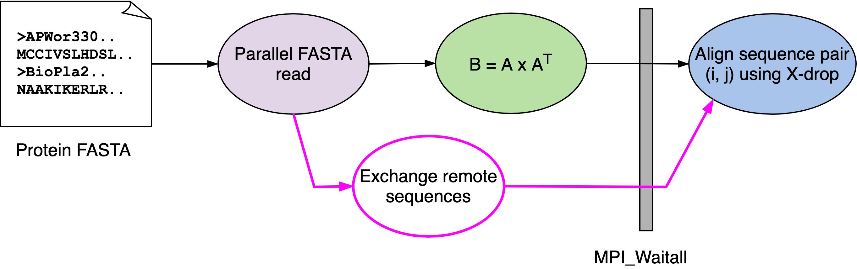
Figure 10: Overlapping communication and computation in PASTIS.

We can avoid both of these and move computation to data for free since $\mathbf{B}$ is symmetric. This is shown in Figure 11. Note all processes except the off-diagonal ones in the last row and column of the figure are square blocks. Despite their dimensions, we see that all the pairs in the upper triangular portion of $\mathbf{B}$ are equivalent to the collection of pairs in individual upper triangular portions of each process block.

For example, the matrix at the left of Figure 11 shows that $\mathrm{P5}$ should compute all nonzero pairs in its row and column sequence ranges. At right, we show that this is equivalent to $\mathrm{P5}$ computing nonzero pairs in its upper triangular and $\mathrm{P7}$ computing nonzero pairs in its upper triangular. Also note that the diagonal entries of each block will only be computed by processes on or above the main diagonal, i.e., $\mathrm{P0,P1,P2,P4,P5,P7}$.

VI Evaluation

We present our evaluation in two categories: parallel performance and relevance. We use different set(s) of data in each. In the former category, we use subsets of Metaclust50 [25] dataset. Originally, this dataset has a total of 313 million sequences and we use random subsets of different sizes in our evaluation: 0.5, 1, 1.25, 2.5, and 5 million sequences, depending on the setting of the experiment. We indicate the subset size within the evaluated dataset, e.g., Metaclust50-0.5M for a subset of 0.5 million sequences. In the latter category, we use the curated (a combination of automatic and manual curation) dataset SCOPe (Structural Classification of Proteins – extended) [26] to measure precision and sensitivity. From the original set of 243,813 proteins in this dataset, we pick 77,040 unique proteins. SCOPe dataset has 4,899 protein families. In the relevance evaluation, we compare PASTIS against MMseqs2 [3], a many-against-many sequence searching and clustering software for large protein and nucleotide sequence sets, and LAST [5], an aligner with an emphasis on discovering weak similarities. The evaluation and discussions for the two categories are presented in Section VI-A and VI-B, respectively.

We conduct our evaluations on NERSC Cori system - a Cray XC40 machine. Each Haswell node on this system consists of two 2.3 GHz 16-core Intel Xeon E5-2698 v3 processors and has a 128 GB of total memory. Each KNL node consists of a single 1.4 GHz 68-core Intel Xeon Phi 7250 processor and has 96 GB of total memory. We use Haswell nodes in our comparisons against MMseqs2 and LAST, while we use KNL nodes in analyzing scalability of PASTIS. The KNL partition of Cori has more nodes and hence it allows larger-scale experiments. Given MMseqs2 does not support AVX512, the comparison against it is run on Haswell nodes with AVX2 instructions for a fair comparison.

Both PASTIS and MMseqs2 support hybrid MPI and OpenMP parallelism. For both tools, we assign each node a single MPI task with as many threads as there are cores on the node. Both tools are compiled with gcc 8.3.0 and the O3 flag. In our evaluations, both MMseqs2 and the SeqAn library used for alignment in PASTIS make use of vectorization with Advanced Vector Extensions 2 (AVX2), while LAST uses SSE4.

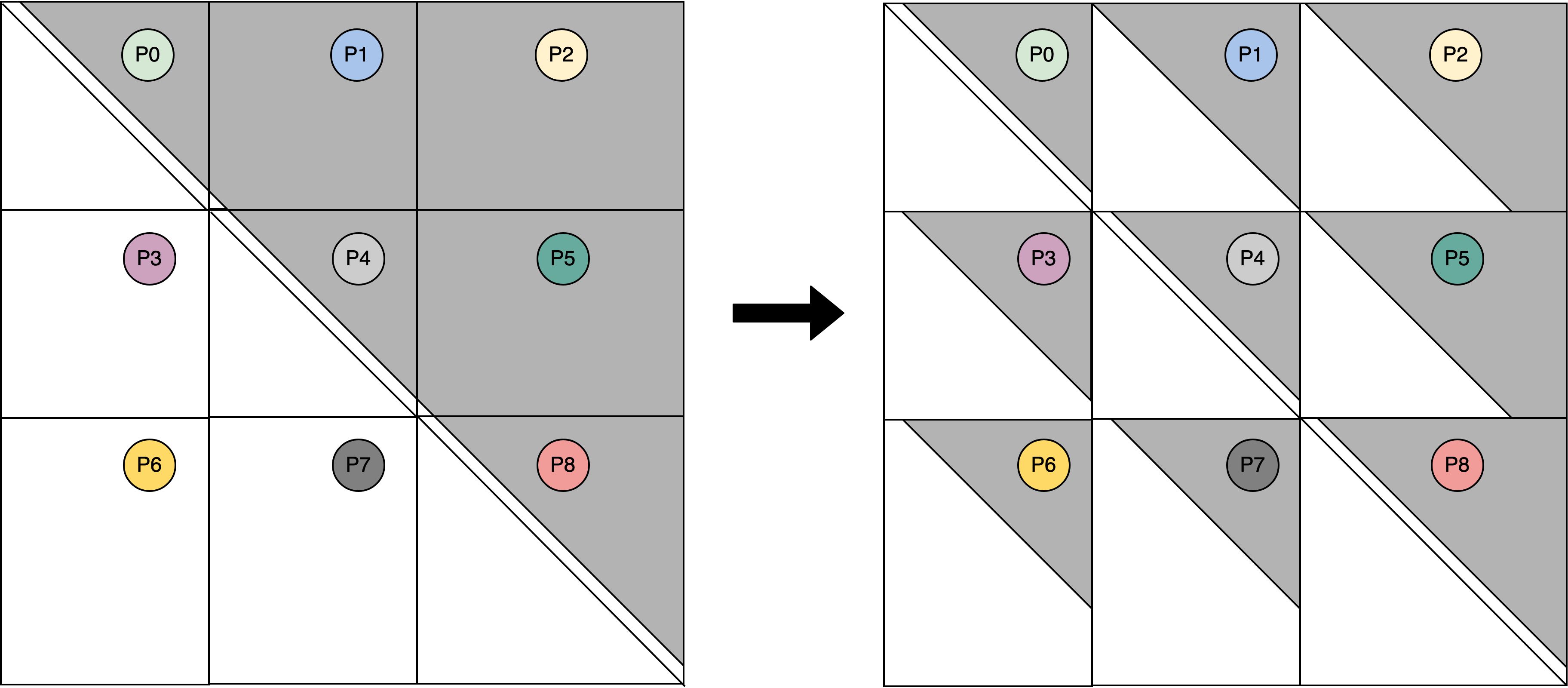
Figure 11: Distribution of computation over data.

Both alignment modes described in Section IV-E are used in our evaluation of PASTIS. To indicate these modes, we add the alignment modes’ abbreviations as a suffix to our tool, e.g., PASTIS-SW or PASTIS-XD. For XD alignment, we use an x-drop value of 49. We use a k-mer size of 6 for PASTIS. For PASTIS, we also evaluate a parameter called common k-mer threshold. When this parameter is set to t, we eliminate (i.e., do not perform alignment on) read pairs that share t or fewer $k$-mers. For exact k-mers we use a common k-mer threshold of 1 and for substitute k-mers we use a common k-mer threshold of 3. The variants of PASTIS with this parameter are indicated with CK suffix. During the pairwise alignment, we use the BLOSUM62 substitution matrix [22] with a gap opening cost of 11 and a gap extension cost of 1. For MMseqs2 and LAST, we use the default settings except for the sensitivity, identity score and coverage thresholds, which change according to the experiment setup as described later. Note that LAST’s parallelism is constrained to a single node. Nonetheless, we include it in our evaluation mainly for sensitivity comparison, although we also report its single-node runtime performance.

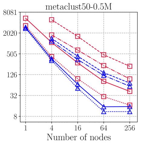
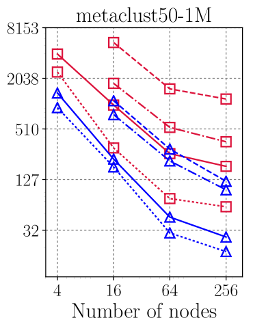
Figure 12: Runtime of PASTIS variants on two datasets. The y-axis denotes the execution time in seconds.

VI-A Parallel Performance

First, we evaluate parallel performance of PASTIS by comparing it against another distributed memory aligner MMseqs2 and shared memory aligner LAST. Then, we focus on scaling aspects and investigate how different components of PASTIS scale.

Comparison against MMseqs2 and LAST. For the comparison we use two datasets with 0.5 and 1 million sequences. We vary the number of nodes from 1 to 256, increasing it by a factor of 4. Additionally, we evaluate a number of different options for PASTIS. For the alignment, we test SW and XD. For substitute k-mers we use the values of 0 (i.e., there is no $\mathbf{S}$ matrix) and 25. These are indicated with suffixes to PASTIS. For MMseqs2, we test out three different sensitivity settings (parameter $s$): low (1.0), default (5.7), and high (7.5). A smaller sensitivity value should result in a faster execution for MMseqs2. For LAST, we use 100 for the maximum initial matches per query position. This parameter controls the sensitivity and the higher it is, the more time LAST takes. Figure 12 compares PASTIS variants among themselves and Figure 13 shows the execution time of the fastest variant of PASTIS, MMseqs2, and LAST. The missing data points for PASTIS are due to running out of memory.

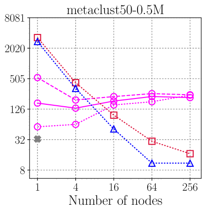
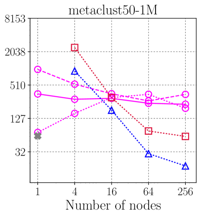
Figure 13: Runtime of PASTIS vs. MMseqs2 on two datasets. The y-axis denotes the execution time in seconds.

When we compare different variants of PASTIS in Figure 12, we can see that using substitute k-mers increases the execution time as expected because we add the substitution matrix to the sparse matrix computations and increase the number of alignments. For instance, in Metaclust50-0.5M, the number of alignments performed with exact k-mers is 399 million whereas with 25 substitute k-mers it is 3.5 billion – amounting to a factor of 8.7$\times$ in the number of alignments. XD is substantially faster than SW, without any significant change in accuracy (we discuss this in Section VI-B). The PASTIS variants that use the common k-mer threshold are faster as they perform fewer alignments than their counterparts.

Figure 13 shows that PASTIS is slower than MMseqs2 for small node counts but, due to its better scalability, it is able to close the performance gap rather quickly. PASTIS-XD-s0-CK runs faster than MMseqs2 in both datasets starting around 16 nodes. PASTIS often scales favorably. We investigated the unscalable behavior of MMseqs2 and found out that although the computations scale well, the processing after running the alignments constitutes bulk of the time and causes a bottleneck. In that processing stage, MMseqs2 probably gathers alignment results from other nodes in order to write the output using a single process, which is handled in parallel in PASTIS. Among different variants of MMseqs2, MMseqs2-low runs faster as expected in a single-node setting. However, MMseqs2-high scales somewhat better as it is more compute-bound than the two other variants. LAST’s single-node performance is better than three variants of MMseqs2.

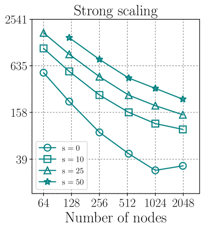
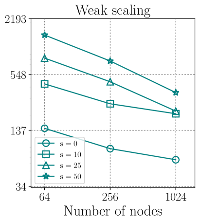
Figure 14: Strong-scaling (left) and weak-scaling (right) performance of PASTIS. The y-axis is the execution time in seconds.

The percentage of time spent in aligning pairs in PASTIS is presented in Table I. The alignment percentages are higher for SW as it is more expensive than XD. Increasing the number of sequences from 0.5 million to 1 million causes a quadratic increase in the number of aligned pairs (will be discussed shortly), while sparse matrix operations usually scale linearly. Hence, the percentage of time spent in alignment tends to increase with increased number of sequences.

Strong and Weak Scaling. In this section, we solely focus on the sparse matrix operations and exclude alignment. The alignment computations are independent of each other and each process computes its portion of alignments without requiring any coordination or synchronization with other processes. The local alignments at a process are also highly parallel as aligned pairs are also independent of each other. Conversely, the sparse matrix computations have different flavors and accommodate more challenges in terms of parallelization. Hence, we only focus on the scalability of PASTIS without alignment of sequence pairs. The experiments in this section are performed on the KNL partition of Cori to exploit a larger number of nodes.

On the left side of Figure 14, we illustrate the strong scaling behavior on Metaclust50-2.5M with number of substitute k-mers $\{0,10,25,50\}$, and the number of nodes $\{64,121,256,529,1024,2025\}$. The odd number of nodes is due to perfect square process count requirement in PASTIS. We choose the perfect square integer closest to the target process count. Figure 14 shows that using exact k-mers exhibits better scalability than using substitute k-mers up to 2K nodes. Substitute k-mers exhibit similar scalability among themselves with an increase in runtime as the number of substitutions increases. The substitute k-mers implementation requires formation of the substitution matrix $\mathbf{S}$, an additional SpGEMM, and the symmetrization of the similarity matrix. These components seem to be less scalable compared other components.

On the right side of Figure 14, we illustrate the weak scaling behavior. We use three different datasets: Metaclust50-1.25M at 64 nodes, Metaclust50-2.5M at 256 nodes, and Metaclust50-5M at 1024 nodes. We observe that the number of nonzeros in the output matrix increases roughly by a factor of four when we double the number of sequences. For example, for 25 substitute k-mers, the output matrices resulting from using 1.25M, 2.5M, and 5M sequences respectively contain 10.9, 43.3, and 172.3 billion nonzeros. The lines in the weak scaling plots have a negative slope, which may seem unrealistic. However, not all operations scale with a quadratic factor. For example, some operations such as communicating sequences and generating substitute k-mers scale linearly with the number of processes. Consequently, a weak-scaling line with a negative slope may be expected as we increase the number of nodes with a factor of four. On the other hand, a factor of two would result in lines with a positive slope.

TABLE I: Alignment time percentage in PASTIS.

	Metaclust50-0.5M					Metaclust50-1M
Scheme	1	4	16	64	256	1	4	16	64	256
PASTIS-SW-s0	49%	83%	89%	91%	81%	-	73%	91%	94%	71%
PASTIS-SW-s25	-	80%	81%	78%	75%	-	-	90%	89%	94%
PASTIS-XD-s0	7%	54%	55%	55%	52%	-	51%	59%	64%	50%
PASTIS-XD-s25	-	31%	29%	25%	27%	-	-	50%	40%	39%
PASTIS-SW-s0-CK	12%	60%	69%	77%	64%	-	58%	71%	77%	62%
PASTIS-SW-s25-CK	-	44%	53%	51%	48%	-	-	68%	66%	69%
PASTIS-XD-s0-CK	1%	48%	44%	34%	33%	-	48%	47%	44%	36%
PASTIS-XD-s25-CK	-	17%	11%	6%	7%	-	-	25%	15%	12%

Dissection Analysis. In this section, we examine the time spent in various components of PASTIS and how these components scale. As in the previous section, we exclude alignment from our analysis. We measure the time of 5 different components when exact k-mers are used and 8 different components when substitute k-mers are used. Figure 15 shows the obtained results. The components that are specific to substitute k-mers are (i) the formation of $\mathbf{S}$, (ii) $\mathbf{A}\mathbf{S}$, and (iii) the symmetrization. The last component is required to make the output matrix symmetric. The “fasta.”, “tr. $\mathbf{A}$”, and “wait” components respectively stand for reading/processing of fasta data, computing $\mathbf{A}^{\mbox{\scriptsize\sf T}}$, and waiting for the communication of sequence data to be completed (Section V-C).

Figure 15 shows that waiting for the sequence transfers to complete constitutes a considerable portion of the overall time, especially at small node counts. This component is less pronounced when substitute k-mers are used as other components take more time while the sequence transfer time stays the same. For the exact k-mers, the most computationally dominant component is the SpGEMM, whereas for the substitute k-mers, SpGEMM and the formation of $\mathbf{S}$ dominate the computation. The formation of $\mathbf{A}$ or $\mathbf{S}$ often takes less time than the SpGEMMs at the smaller node counts. However, with increasing number of nodes, the percentage of time spent in SpGEMM increases as opposed to that of matrix formation, which indicates that SpGEMM is less scalable.

In Figure 16, we investigate how each component of PASTIS scales. The results in the plot at the top are obtained with Metaclust50-2.5M with exact k-mers and the results in the plot at the bottom are obtained with the same dataset with 25 substitute k-mers. In both plots, the bottleneck for scalability seems to be the SpGEMM operations. Other components either take too short time or scale relatively better.

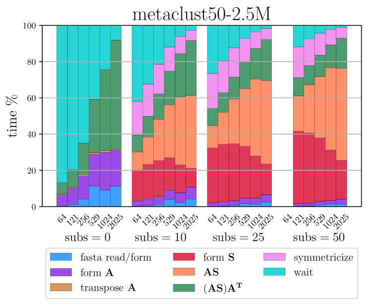
Figure 15: Percentage of time spent in various components of PASTIS plotted against increasing number of nodes for different number of substitute k-mers.

VI-B Precision and Recall

In our evaluation, PASTIS, MMseqs2, and LAST perform alignment and generate alignment statistics for sequence pairs to form the similarity graph $G$. Then, $G$ is clustered with High-performance Markov Clustering (HipMCL) [9] to discover possible protein families. To determine the edge weights in $G$, we use two different similarity measures: Average Nucleotide Identity (ANI) and Normalized Raw Alignment Score (NS). When we use ANI, the alignments with ANI less than 30% and shorter sequence coverage less than 70% are eliminated from the similarity graph and the edge weight $w(s_{i},s_{j})$ is set to the ANI of sequences $s_{i}$ and $s_{j}$.

In NS, we use the raw alignment score normalized with respect to the shorter sequence. A motivation for this is that computing NS score is cheaper than ANI as the former does not necessitate a trace-back step in the alignment. Although NS may not be as accurate as ANI, it still accommodates a rough information that the clustering algorithm can effectively make use of. We use a number of different substitute k-mers $\{0,10,25,50\}$ for PASTIS to measure its effect on the quality of the clusters. Similarly, we utilize sensitivity values $\{1,5.7,7.5\}$ for MMseqs2 and $\{100,200,300\}$ for LAST. The default for the sensitivity is 5.7 in MMseqs2.

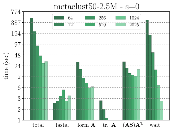
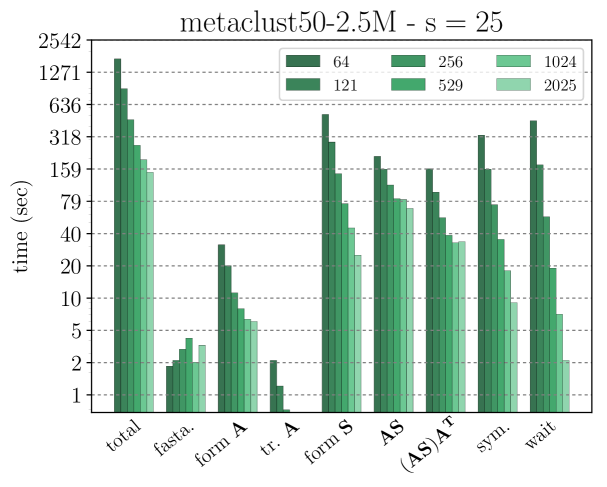
Figure 16: Scaling behavior of various components.

To compute precision and recall, we use the clusters produced by HipMCL against the protein families in SCOPe dataset. Particularly, we use weighted precision and recall as defined in the protein clustering studies [27]. The weighted precision metric penalizes clusters that contain proteins from multiple families while the weighted recall metric penalizes clusters that are split into multiple families. Figure 17 shows the values obtained by the compared schemes in terms of weighted precision and recall. As an important note, the precision range in Figure 17 is between 0.65 and 0.90, and the recall range is between 0.48 and 0.62.

Figure 17 shows that one can use different number of substitute k-mers to adjust the sensitivity, where increasing the number of substitute k-mers increases recall at the expense of precision. In the figure, the range in which the precision and recall vary is somewhat limited. We note that a more comprehensive spectrum can be obtained by altering the parameters given to SeqAn. Except for PASTIS-SW-NS, PASTIS shows competitive performance compared to MMseqs2 and LAST.

Comparing SW and XD with fixed parameters except for the alignment mode shows that utilizing SW achieves slightly better recall at the expense of slightly, or sometimes substantially, worse precision. A second important point is that NS proves to be viable compared to the ANI score. This is especially the case for PASTIS with XD alignment and MMseqs2. However, PASTIS with SW alignment seems to be more sensitive to NS. Notably, we do not apply any cut-off threshold when using NS in the similarity graph. Hence, while XD may be able to eliminate some of the low-score alignments, this is not the case for SW. Alignment libraries aside, the clustering algorithm (Markov Clustering in our case) may also be playing an important role in closing the quality gap between different weighting schemes used for the edges in the similarity graph.

The common k-mer threshold causes a 2%-3% loss in recall. This loss is arguably small when weighted against the benefits it brings in runtime. In many cases, applying this threshold results in more than 90% reduction in the alignments PASTIS performs and leads to drastic gains in parallel runtime.

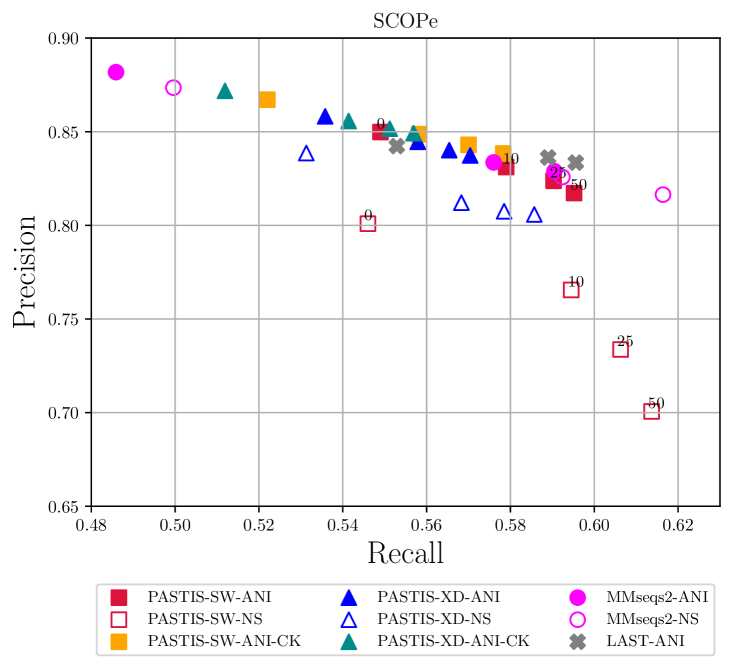
Figure 17: Precision and recall of PASTIS, MMseqs2, and LAST for various parameters. The annotation text (over PASTIS-SW-ANI and PASTIS-SW-NS) indicate the number of substitute k-mers utilized in the corresponding setting. They are omitted for PASTIS-XD variants in order to make the figure readable. The sensitivity parameters for MMseqs2 variants range from left to right as 1 (low), 5.7 (default), 7.5 (high). The sensitivity parameters for LAST range from left to right as 100, 300, 500.

In Table II, we investigate the effect of directly using connected components of the similarity graph as protein families. Here, the alignments with less than 30% ANI score and less than 70% coverage are eliminated. The connected components might be appealing to avoid running an expensive clustering algorithm. Components generated using MMseqs2 and LAST exhibit higher quality than the ones generated by PASTIS. On one hand, using substitute k-mers without clustering causes substantial precision penalty as the number of connected components gets very small with increasing number of substitute k-mers. Therefore, clustering is indispensable when substitute k-mers are used within PASTIS. On the other hand, PASTIS with exact k-mers may be a viable option when clustering cannot be performed.

VII Conclusion

We developed a scalable approach to protein similarity search within our software PASTIS. PASTIS harnesses the expressive power of sparse matrix operations and those operations’ strong parallel performance to enable construction of huge protein similarity networks on thousands of nodes in parallel. The substitute k-mers in PASTIS facilitate better recall and enables controlling sensitivity. With several optimizations, PASTIS illustrates how linear algebra can provide a flexible medium to tackle problems in computational biology that deal with huge datasets and require resources that cannot be met with small- or medium-scale clusters.

Unlocking the true power of distributed-memory supercomputers for protein sequence similarity search will help accelerate the mining of functional and taxonomical diversity of the protein world, especially when analyzing large metagenomic datasets. Identification of biosynthetic gene clusters [28], discovery of novel protein families [29], uncovering the world of viruses [30], and routine functional [31] and taxonomical [32] classification from large metagenomic samples all depend on the ability to perform protein sequence similarity search at scale. PASTIS is a step towards enabling new biological discoveries at extreme scale using the fastest supercomputers. One of the next major milestones in PASTIS development is to take advantage of accelerators such as GPUs in distributed-memory protein sequence similarity search.

As future work, we first plan to address the issues related to memory requirements of PASTIS as it occasionally runs out of memory at small node counts. A direction in this regard is the partial formation of the output matrix and once this partial information is obtained to run the alignment and free the corresponding memory. Another future avenue is to perform an analysis of k-mers in a pre-processing stage to see whether some of them can be eliminated without sacrificing recall too much. We also plan to conduct an performance analysis of enhanced pipeline with clustering.

TABLE II: Connected components as protein families.

		Number of substitute k-mers
		0	10	25	50
PASTIS-SW	precision	0.67	0.38	0.28	0.22
	recall	0.67	0.77	0.83	0.87
PASTIS-XD	precision	0.69	0.55	0.46	0.39
	recall	0.64	0.69	0.73	0.76

		Sensitivity
		1	5.7	7.5
MMseqs2	precision	0.77	0.75	0.75
	recall	0.60	0.71	0.72

		Max initial matches
		100	200	300
LAST	precision	0.76	0.76	0.76
	recall	0.68	0.70	0.70

References

- [1] W. Li and A. Godzik, “CD-HIT: a fast program for clustering and comparing large sets of protein or nucleotide sequences,” Bioinformatics, vol. 22, no. 13, pp. 1658–1659, 2006.
- [2] R. C. Edgar, “Search and clustering orders of magnitude faster than BLAST,” Bioinformatics, vol. 26, no. 19, pp. 2460–2461, 2010.
- [3] M. Steinegger and J. Söding, “Mmseqs2 enables sensitive protein sequence searching for the analysis of massive data sets,” Nature biotechnology, vol. 35, no. 11, p. 1026, 2017.
- [4] S. F. Altschul, T. L. Madden, A. A. Schäffer, J. Zhang, Z. Zhang, W. Miller, and D. J. Lipman, “Gapped BLAST and PSI-BLAST: a new generation of protein database search programs,” Nucleic acids research, vol. 25, no. 17, pp. 3389–3402, Sep 1997, 9254694[pmid].
- [5] S. M. Kiełbasa, R. Wan, K. Sato, P. Horton, and M. C. Frith, “Adaptive seeds tame genomic sequence comparison.” Genome research, vol. 21, no. 3, pp. 487–93, Mar 2011.
- [6] B. Buchfink, C. Xie, and D. H. Huson, “Fast and sensitive protein alignment using DIAMOND,” Nature methods, vol. 12, no. 1, p. 59, 2015.
- [7] A. J. Enright, S. Van Dongen, and C. A. Ouzounis, “An efficient algorithm for large-scale detection of protein families,” Nucleic acids research, vol. 30, no. 7, pp. 1575–1584, 2002.
- [8] T. Wittkop, D. Emig, S. Lange, S. Rahmann, M. Albrecht, J. H. Morris, S. Böcker, J. Stoye, and J. Baumbach, “Partitioning biological data with transitivity clustering,” Nature methods, vol. 7, no. 6, p. 419, 2010.
- [9] A. Azad, G. A. Pavlopoulos, C. A. Ouzounis, N. C. Kyrpides, and A. Buluç, “HipMCL: a high-performance parallel implementation of the Markov clustering algorithm for large-scale networks,” Nucleic acids research, vol. 46, no. 6, pp. e33–e33, 2018.
- [10] Y. Ruan, S. Ekanayake, M. Rho, H. Tang, S.-H. Bae, J. Qiu, and G. Fox, “DACIDR: Deterministic annealed clustering with interpolative dimension reduction using a large collection of 16s rrna sequences,” in Proceedings of the ACM Conference on Bioinformatics, Computational Biology and Biomedicine, ser. BCB ’12. New York, NY, USA: ACM, 2012, pp. 329–336.
- [11] A. Godzik, “Metagenomics and the protein universe,” Current opinion in structural biology, vol. 21, no. 3, pp. 398–403, 2011.
- [12] A. Buluç and J. R. Gilbert, “The Combinatorial BLAS: Design, implementation, and applications,” The International Journal of High Performance Computing Applications, vol. 25, no. 4, pp. 496–509, 2011.
- [13] A. Buluç and J. R. Gilbert, “Parallel sparse matrix-matrix multiplication and indexing: Implementation and experiments,” SIAM Journal on Scientific Computing, vol. 34, no. 4, pp. C170–C191, 2012.
- [14] Y. Nagasaka, S. Matsuoka, A. Azad, and A. Buluç, “Performance optimization, modeling and analysis of sparse matrix-matrix products on multi-core and many-core processors,” Parallel Computing, vol. 90, p. 102545, 2019.
- [15] E. Solomonik and T. Hoefler, “Sparse tensor algebra as a parallel programming model,” arXiv preprint arXiv:1512.00066, 2015.
- [16] C. Wu, A. Kalyanaraman, and W. R. Cannon, “pgraph: Efficient parallel construction of large-scale protein sequence homology graphs,” IEEE Transactions on Parallel and Distributed Systems, vol. 23, no. 10, pp. 1923–1933, 2012.
- [17] A. Kalyanaraman, S. Aluru, V. Brendel, and S. Kothari, “Space and time efficient parallel algorithms and software for est clustering,” IEEE Transactions on parallel and distributed systems, vol. 14, no. 12, pp. 1209–1221, 2003.
- [18] T. F. Smith, M. S. Waterman et al., “Identification of common molecular subsequences,” Journal of molecular biology, vol. 147, no. 1, pp. 195–197, 1981.
- [19] G. Guidi, M. Ellis, D. Rokhsar, K. Yelick, and A. Buluç, “Bella: Berkeley efficient long-read to long-read aligner and overlapper,” bioRxiv, p. 464420, 2018.
- [20] M. Ellis, G. Guidi, A. Buluç, L. Oliker, and K. Yelick, “dibella: Distributed long read to long read alignment,” in Proceedings of the 48th International Conference on Parallel Processing, 2019, pp. 1–11.
- [21] S. F. Altschul, W. Gish, W. Miller, E. W. Myers, and D. J. Lipman, “Basic local alignment search tool,” Journal of molecular biology, vol. 215, no. 3, pp. 403–410, 1990.
- [22] S. Henikoff and J. G. Henikoff, “Amino acid substitution matrices from protein blocks.” Proceedings of the National Academy of Sciences of the United States of America, vol. 89, no. 22, pp. 10 915–9, Nov 1992.
- [23] A. Buluç and J. R. Gilbert, “On the representation and multiplication of hypersparse matrices,” in IEEE International Symposium on Parallel and Distributed Processing, 2008, pp. 1–11.
- [24] A. Döring, D. Weese, T. Rausch, and K. Reinert, “Seqan an efficient, generic c++ library for sequence analysis.” BMC bioinformatics, vol. 9, p. 11, 2008.
- [25] S. Fayech, N. Essoussi, and M. Limam, “Partitioning clustering algorithms for protein sequence data sets.” BioData mining, vol. 2, no. 1, p. 3, 2009.
- [26] N. K. Fox, S. E. Brenner, and J. M. Chandonia, “SCOPe: Structural Classification of Proteins–extended, integrating SCOP and ASTRAL data and classification of new structures,” Nucleic Acids Res., vol. 42, no. Database issue, pp. D304–309, Jan 2014.
- [27] J. S. Bernardes, F. R. Vieira, L. M. Costa, and G. Zaverucha, “Evaluation and improvements of clustering algorithms for detecting remote homologous protein families,” BMC Bioinformatics, vol. 16, no. 1, p. 34, Feb 2015.
- [28] T. Weber, K. Blin, S. Duddela, D. Krug, H. U. Kim, R. Bruccoleri, S. Y. Lee, M. A. Fischbach, R. Müller, W. Wohlleben et al., “antismash 3.0—a comprehensive resource for the genome mining of biosynthetic gene clusters,” Nucleic acids research, vol. 43, no. W1, pp. W237–W243, 2015.
- [29] H. Sberro, B. J. Fremin, S. Zlitni, F. Edfors, N. Greenfield, M. P. Snyder, G. A. Pavlopoulos, N. C. Kyrpides, and A. S. Bhatt, “Large-scale analyses of human microbiomes reveal thousands of small, novel genes,” Cell, vol. 178, no. 5, pp. 1245–1259, 2019.
- [30] F. Schulz, S. Roux, D. Paez-Espino, S. Jungbluth, D. A. Walsh, V. J. Denef, K. D. McMahon, K. T. Konstantinidis, E. A. Eloe-Fadrosh, N. C. Kyrpides et al., “Giant virus diversity and host interactions through global metagenomics,” Nature, vol. 578, no. 7795, pp. 432–436, 2020.
- [31] E. A. Franzosa, L. J. McIver, G. Rahnavard, L. R. Thompson, M. Schirmer, G. Weingart, K. S. Lipson, R. Knight, J. G. Caporaso, N. Segata et al., “Species-level functional profiling of metagenomes and metatranscriptomes,” Nature methods, vol. 15, no. 11, pp. 962–968, 2018.
- [32] P. Menzel, K. L. Ng, and A. Krogh, “Fast and sensitive taxonomic classification for metagenomics with kaiju,” Nature communications, vol. 7, no. 1, pp. 1–9, 2016.