Study of self-interaction errors in density functional predictions of dipole polarizabilities and ionization energies of water clusters using Perdew-Zunger and locally scaled self-interaction corrected methods
Abstract
We studied the effect of self-interaction error (SIE) on the static dipole polarizabilities of water clusters modelled with three increasingly sophisticated, non-empirical density functional approximations (DFAs), viz. the local spin density approximation (LDA), the Perdew-Burke-Ernzherof (PBE) generalized-gradient approximation (GGA), and the strongly constrained and appropriately normed (SCAN) meta-GGA, using the Perdew-Zunger self-interaction-correction (PZ-SIC) energy functional in the Fermi-Löwdin orbital SIC (FLO-SIC) framework. Our results show that while all three DFAs overestimate the cluster polarizabilities, the description systematically improves from LDA to PBE to SCAN. The self-correlation free SCAN predicts polarizabilities quite accurately with a mean absolute error (MAE) of 0.58 Bohr3 with respect to coupled cluster singles and doubles (CCSD) values. Removing SIE using PZ-SIC correctly reduces the DFA polarizabilities, but over-corrects, resulting in underestimated polarizabilities in SIC-LDA, -PBE, and -SCAN. Finally, we applied a recently proposed local-scaling SIC (LSIC) method using a quasi self-consistent scheme and using the kinetic energy density ratio as an iso-orbital indicator. The results show that the LSIC polarizabilities are in excellent agreement with mean absolute error of 0.08 Bohr3 for LSIC-LDA and 0.06 Bohr3 for LSIC-PBE with most recent CCSD polarizabilities. Likewise, the ionization energy estimates as an absolute of highest occupied energy eigenvalue predicted by LSIC are also in excellent agreement with CCSD(T) ionization energies with MAE of 0.4 eV for LSIC-LDA and 0.04 eV for LSIC-PBE. The LSIC-LDA predictions of ionization energies are comparable to the reported GW ionization energies while the LSIC-PBE ionization energies are more accurate than reported GW results.
I Introduction
Water plays a central role in many areas of science. For that reason, it has been the subject of many computational studies in chemical physics.Ball (2008); Fecko et al. (2003); Wernet et al. (2004); Soper and Benmore (2008); Skinner et al. (2013); Pedroza et al. (2018); Elton and Fernández-Serra (2016); Pedroza et al. (2015); Piaggi and Car (2020); Sommers et al. (2020); Chen et al. (2017); Santra et al. (2015) These studies have led to important insights into the atomic-level behavior of water, but they also allow detailed comparisons of the methods used for the calculations. Generally speaking, ab initio methods at the coupled-cluster level of theory reliably predict the observed properties of water. Density functional theory (DFT) -based methods are more computationally efficient and, with increasing sophistication of the density functional approximation (DFA) used, can give accurate predictions for many properties. Most DFAs, however, are known to over-bind water clusters, particularly at the local density approximations level,Laasonen et al. (1992); Laasonen et al. (1993a); Lee et al. (1994); Laasonen et al. (1993b) fail to correctly predict the structural energy ordering of cluster isomers,Santra et al. (2008); Dahlke et al. (2008) transition pressure for phase transition of ice,Santra et al. (2011) and density in liquid phase.Asthagiri et al. (2003); Grossman et al. (2004); Schwegler et al. (2004) For a recent perspective on the performance of DFT methods for describing water, see Ref. Gillan et al. (2016). The recently developed strongly constrained and appropriately normed (SCAN) meta-GGASun et al. (2015) further improves the description of water clusters, liquid water, and ice,Sun et al. (2016); Chen et al. (2017) but shortcomings such as over-binding tendency remain. We recently showed that much of the over-binding can be eliminated by removing self-interaction error (SIE) from the DFA. SIE is caused by an incomplete cancellation of self-Coulomb and self-exchange energies in the DFA. The Perdew-Zunger self-interaction correctionMiliordos et al. (2013) (PZ-SIC) removes the self-interaction on an orbital by orbital basis. Using the PZ-SIC energy functional in the Fermi-Löwdin orbital self-interaction correction (FLO-SIC) method to remove self-interaction, we showed that the overbinding in SCANSun et al. (2015) is reduced by a factor of 3 to about 10 meV per molecule in small water clusters.Sharkas et al. (2020) Furthermore, SCAN is known to predict the correct energetic ordering of the isomers of the water hexamer, a celebrated test for DFAs, and this is not changed in the FLO-SIC-SCAN calculations.
Because water is a polar solvent, its dielectric properties are important. Several ab initio and DFT calculations have examined how the dipole moments and static dipole polarizabilities of (H2O)n clusters evolve with , Jensen et al. (2002); Tu and Laaksonen (2000); Ghanty and Ghosh (2003); Yang et al. (2005, 2010); Krishtal et al. (2006) as well as how these properties can be broken into many-body contributions.Medders and Paesani (2013) Hammond et al. carried out calculations of the dipole polarizability of water clusters up to at the coupled-cluster level of theoryHammond et al. (2009) and using several DFAs, using cluster geometries optimized at the MP2 level.Xantheas (1996); Xantheas et al. (2002) By carefully studying details such as the effect of basis set and the level of theory, their results provide excellent reference values. Similarly, Alipour and co-workers studied water cluster polarizabilities with coupled-cluster and hybrid and double hybrid DFT methods.Alipour (2013); Alipour and Fallahzadeh (2017) While these last two studies shed some light on how DFT-based methods perform for dielectric properties, they do not directly address the effect of SIE. That is the topic of this paper.
It is clear that SIE should impact calculated dipoles and polarizabilities. A well-known effect of electron self-interaction is that the potential “seen” by electrons is too-repulsive in the asymptotic region of a neutral system, decaying exponentially to zero, rather than with the correct dependence. The result is that electrons are too loosely bound in a DFA calculation, as can be seen, for example, in orbital energies that are too high in comparison with removal energies.Jackson et al. (2019) Similarly, in calculations of atomic anions, the highest occupied electronic states have positive orbital energies, implying that the anions are actually unstable. Removing self-interaction via FLO-SIC calculations restores the correct asymptotic behavior of the potential and improves the description of related properties. In a recent study of water cluster anions,Vargas et al. (2020) for example, we showed that FLO-SIC significantly improves the prediction of vertical detachment energies (VDEs). For clusters up to the hexamer, the orbital energy for the highest state in FLO-SIC-PBE predicted the corresponding VDE with a mean average error of only 17 meV compared to CCSD(T) values. In the context of molecular dipoles, the effect of self-interaction is to destabilize the anionic part of a molecule relative to the cationic part, resulting in too little charge transfer and dipoles that are too small. Removing self-interaction from a large test set of molecules improved the calculated dipole moments, though the corrections tended to be too large, yielding dipoles that are somewhat too large compared to reference values. On the other hand, electrons that are too loosely bound respond too strongly to an applied electric field, leading to polarizabilities that are too large. In a study of neutral and singly charged atoms,Withanage et al. (2019) removing self-interaction generally reduces the predicted polarizabilities, improving agreement with experimental values. But in this case, too, FLO-SIC tends to over-correct, resulting in predictions that underestimate experiment.
Here we report the results of using FLO-SIC-DFA methods to compute the dipole moments and polarizabilities for (H2O)n clusters up to . We have used three increasingly sophisticated,Perdew and Schmidt (2001) non-empirical DFAs for our study — the LDA in the Perdew-Wang version, the Perdew, Burke, and Ernzerhof (PBE) GGA,Perdew et al. (1996) and SCAN.Sun et al. (2015) We find that removing SIE increases calculated dipole moments and decreases polarizabilities. We also show that the FLO-SIC corrections overshoot the relevant reference values. A second objective of this paper is therefore to show the performance of a recent local-scaling self-interaction correctionZope et al. (2019) (LSIC) method for the prediction of dipoles and polarizabilities. LSIC uses a position-dependent factor based on the local character of the charge density to scale down the energy densities of the SIC. We show that a quasi-self-consistent implementation of LSIC reduces the over-correction of polarizabilities and yields calculated values that are in the best agreement of all the DFT-based methods with reference values.
II Methods and Computational Details
The Fermi-Löwdin orbital-based self-interaction correction (FLO-SIC) methodPederson et al. (2014); Pederson (2015); Yang et al. (2017); Pederson and Baruah (2015) is used for the calculations presented here. It is implemented in the FLO-SIC codeZope et al. which is based on the UTEP version of the NRLMOL code. FLO-SIC retains the principal features of NRLMOL, including optimized Gaussian basis functionsPorezag and Pederson (1999) and a highly accurate numerical integration grid scheme.Pederson and Jackson (1990)
FLO-SIC makes use of the orbital-dependent PZ-SIC energy functional. Unlike for DFAs, where the energy depends only on the total density and any unitary transformation of the orbital wave functions yields the same energy, minimizing the PZ-SIC total energy requires optimizing both the total density and the choice of orbitals used to evaluate the energy. In FLO-SIC, localized Fermi-Löwdin orbitals (FLOs) are used.Pederson et al. (2014) Fermi orbitals are first constructed as follows,
| (1) |
Here and are the orbital indices, is the spin index, is the electron density, and the are any set of orbitals that span the occupied space. In practice, the canonical orbitals are typically used. is a position in space called a Fermi orbital descriptor (FOD). One such FOD is required for each Fermi orbital. The Fermi orbitals resulting from Eq. (1) are normalized but not mutually orthogonal. They are orthogonalized using the Löwdin symmetric orthogonalization scheme.Löwdin (1950)
As shown in Ref. Pederson (2015); Pederson and Baruah (2015), the derivatives of the total energy with respect to the FOD components can be computed, and these FOD “forces” can be used in a gradient-based minimization scheme to determine the optimal orbitals. We note that the process of finding the optimal FOD positions compares to finding the O() elements of an optimal unitary transformation between canonical and localized orbitals in traditional PZ-SIC calculations.Pederson et al. (2014, 1984, 1985)
In LSIC,Zope et al. (2019) the exchange-correlation energy for a specific DFA is written as
| (2) |
where
| (3) |
| (4) |
Here the scaling factor lies between 0 and 1 and indicates the nature of the charge density at . for a density corresponding to a single electron orbital and for a uniform density. Scaling the self-interaction correction terms with thus retains the full correction for one-electron densities, making the theory exact in that limit, and eliminates the correction in the limit of a uniform density where is exact. As mentioned by Zope et al.Zope et al. (2019) any iso-orbital indicator that can identity the single-electron region can be used in the LSIC method. We will refer this LSIC method as LSIC() to indicate use of LSIC method with kinetic energy density ratio as iso-orbital indicator. Using the pointwise LSIC correction results in significant improvement in electronic properties over SIC-LDA, particularly in situations where atoms are near the equilibrium positions and PZ-SIC performs poorly.
LSIC earlier was employed in a non-variational manner on self-consistent PZ-SIC density.Zope et al. (2019) For calculation of polarizabilities it is necessary to capture the density variation in response to an applied electric field. We used a quasi-self-consistent approach (like in SOSICYamamoto et al. (2020)) using the following Hamiltonian:
| (5) |
This Hamiltonian ignores the density dependence of scaling factor and can be viewed analogous to the model exchange (-correlation) potentials designed to provide accurate excitation energies or polarizabilities.Van Leeuwen and Baerends (1994); Van Gisbergen et al. (2001); Grüning et al. (2002); Banerjee et al. (2007, 2008); Schipper et al. (2000) Although this approach ignores the full variation of the LSIC term, we expect most effects of self-consistency (as in orbital-dependent-SICYamamoto et al. (2020)) are captured using the scaled SIC potentials.
The static dipole polarizability tensor is defined from change in the total energy of a system under an applied static electric field as
| (6) | |||||
| (7) |
where is the energy at zero electric field and and are the component of the dipole moment and the applied electric field. We compute the components of the polarizability tensor using the finite-difference formula as follows
| (8) |
The finite difference calculation of polarizability using the dipole has been proven to be more accurate than the sum-over-states perturbation method.Zope et al. (2008) Electric fields of strength 0.005 a.u. were applied in , , and directions to determine the components of the polarizability tensor for each cluster. The average polarizability is calculated from the trace of the polarizability tensor as
| (9) |
The anisotropy of the polarizability tensor is calculated as
| (10) |
The standard Gaussian orbital basis sets used in the NRLMOL and FLO-SIC codes are optimized for the PBE functionalPerdew et al. (1996) and are of quadruple zeta quality.Schwalbe et al. (2018) For H (O), the standard basis set includes 4 (5) s-type, 3 (4) p-type, and 1 (3) (Cartesian) d-type orbitals, contracted from a set of 7 (14) single Gaussian orbitals (SGO). For polarizability calculations, we used an additional SGO polarization function for each angular moment type.
We used non-empirical functionals from the lowest three rungs of Jacob’s ladder to compute polarizabilities with and without SIC: LDA as parameterized in PW92,Perdew and Wang (1992) PBE,Perdew et al. (1996) and SCAN.Sun et al. (2015) Calculations with SCAN require a particularly fine grid for numerical accuracy.Yamamoto et al. (2019) For example, for water hexamer isomers, the SCAN grid contains roughly twice the number of points than the grid needed for LDA and PBE.
III Results and Discussion
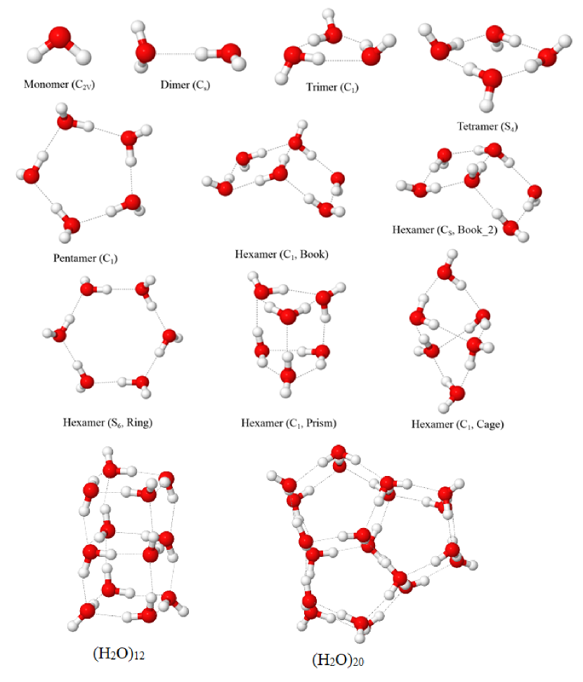
We used the geometries of the water clusters optimized at the CCSD(T) level of theory by Miliordos et al..Miliordos et al. (2013) This set of clusters contains one isomer each for the monomer to pentamer, and five isomers for the water hexamer. Two larger clusters of twelve and twenty water molecules optimized at the MP2/aug-cc-PVTZ levelRakshit et al. (2019) are also included in this set. The cluster structures are shown in Fig. 1. The hexamers are labeled according to shape as prism (p), ring (r), book1 (b1), book2 (b2), and cage (c). The binding energies of the water hexamers found here follow the ordering reported in Ref. Sharkas et al. (2020). The stability ordering using LDA, SCAN, FLO-SIC-LDA, and FLO-SIC-SCAN from the most stable to the least is pcb1b2r whereas using PBE and FLO-SIC-PBE the ordering is b1rcpb2.
We optimized the positions of the FODs independently for FLO-SIC-LDA, FLO-SIC-PBE, and FLO-SIC-SCAN calculations. In addition, because the electron distribution may change with application of an external field, we re-optimized the FOD positions when an external field was applied, using the zero-field positions as starting points. We find that the FOD positions generally relax in the direction opposite to the applied electric field. This shift in position is small, for example, when a static electric field of strength 0.005 a.u. is applied where the largest shift in position of FOD is 0.2 Å. Re-optimizing the FOD positions has a relatively small effect on the value of the calculated polarizability. For example, in FLO-SIC-PBE, the polarizability of the monomer changes from 8.34 Bohr3 using the zero-field FODs for all calculations, to 8.55 Bohr3 using FODs that are optimized for each applied field. For hexamers, the average change in polarizability arising from FOD optimization ranges from 1.8 to 2.2% with LDA and PBE, respectively. As can be seen below, this difference is small compared to the differences between DFA and FLO-SIC-DFA results.
| Water | DFA | FLO-SIC | LSIC() | MP2111Reference [Gregory et al., 1997] | |||||
|---|---|---|---|---|---|---|---|---|---|
| cluster | LDA | PBE | SCAN | LDA | PBE | SCAN | LDA | PBE | |
| 1 | 1.90 | 1.84 | 1.88 | 2.00 | 1.94 | 1.97 | 1.87 | 1.84 | 1.868 |
| 2 | 2.71 | 2.62 | 2.63 | 2.74 | 2.68 | 2.70 | 2.61 | 2.58 | 2.683 |
| 3 | 1.08 | 1.05 | 1.07 | 1.15 | 1.12 | 1.13 | 1.09 | 1.07 | 1.071 |
| 4 | 0.00 | 0.00 | 0.00 | 0.00 | 0.00 | 0.00 | 0.00 | 0.00 | 0.00 |
| 5 | 1.01 | 0.98 | 1.00 | 1.07 | 1.04 | 1.05 | 1.01 | 1.00 | 0.927 |
| 6p | 2.68 | 2.59 | 2.62 | 2.77 | 2.69 | 2.72 | 2.61 | 2.57 | 2.701 |
| 6c | 2.08 | 2.01 | 2.03 | 2.13 | 2.07 | 2.10 | 2.00 | 1.97 | 1.904 |
| 6b1 | 2.55 | 2.46 | 2.49 | 2.63 | 2.55 | 2.57 | 2.46 | 2.42 | – |
| 6b2 | 2.59 | 2.50 | 2.53 | 2.69 | 2.60 | 2.62 | 2.51 | 2.46 | – |
| 6r | 0.00 | 0.00 | 0.00 | 0.00 | 0.00 | 0.00 | 0.00 | 0.00 | 0.00 |
| 12 | 0.00 | 0.00 | 0.00 | 0.00 | 0.00 | – | 0.00 | – | – |
| 20 | 0.28 | 0.28 | 0.29 | 0.30 | – | – | 0.30 | – | – |
| MAE | 0.04 | 0.05 | 0.04 | 0.09 | 0.05 | 0.06 | 0.05 | 0.05 | |
The zero-field static dipole moments calculated for the clusters are presented in Table 1. Gregory et al. calculated the dipole moments of small water clusters up to using the MP2 theory and aug-cc-VDZ basis sets.Gregory et al. (1997) These are included for reference in Table 1. We emphasize that although there are small differences in the geometries of the reference set and ours, these comparisons can still show the trend of dipole moments with different DFAs with FLO-SIC and LSIC(). The application of FLO-SIC increases the size of non-zero dipole moments in the water clusters compared to DFA calculations. Similar observations were made in an earlier FLO-SIC application to a diverse set of molecules.Johnson et al. (2019) This effect can be understood considering the effect that SIC has on the potential seen by the electrons. By removing the interaction of an electron with itself, SIC makes the potential more attractive. For example, for a neutral atom or molecule, the DFA potential decays exponentially to zero in the asymptotic region. SIC corrects this unphysical behavior, restoring the correct form. In a heteronuclear molecule, this tends to stabilize the anionic part relative to the cationic part, giving rise to larger dipoles. In Table 1, the FLO-SIC-DFA dipoles are between and D larger than the corresponding DFA values in all cases except for the tetramer, the ring hexamer, and the 12-molecule water that have exactly zero dipole moments due to their symmetry. The directions of the dipoles of the water clusters remained nearly same in all clusters with DFA and FLO-SIC-DFA.
The water cluster dipole moments were also calculated using the recently developed LSIC() approach with LDA and PBEZope et al. (2019) functionals. For the monomer the LDA/FLO-SIC-LDA dipole moments are 1.90 D and 2.00 D, respectively, while LSIC()-LDA results in a value of 1.87 D, much closer to the experimental value of 1.855 D.Lovas (1978) The dipole moments for the dimer with PBE and SCAN are close to the experimental value of 2.643 DDyke et al. (1977) which increase to 2.68 D and 2.70 D with SIC. In this case LSIC()-LDA predicts a somewhat smaller value of 2.61 D, but much closer to the experimental value than the FLO-SIC-LDA value (2.74 D). On the whole, the LSIC()-LDA dipole values have a MAE of 0.05 D, a significant improvement over FLO-SIC-LDA (0.09 D), but similar to the other methods. Surprisingly, the LSIC()-LDA values are generally smaller than the LDA values. A possible explanation for this is that the density near the H atoms in a water cluster is dominated by the H 1s orbital and is thus one-electron-like. Thus, full SIC is expected in the region near the H atoms, whereas a reduced SIC is expected near the O atoms, effectively lowering the potential seen by an electron near the H atoms relative to that near O. The net effect of this may be to shift electron charge toward the H atoms, resulting in smaller dipoles. This effect is currently under further investigation.
| Water | DFA | FLO-SIC | LSIC() | CCSDa | CCSDb | |||||
|---|---|---|---|---|---|---|---|---|---|---|
| cluster | LDA | PBE | SCAN | LDA | PBE | SCAN | LDA | PBE | ||
| 1 | 10.63 | 10.58 | 10.04 | 8.43 | 8.55 | 8.69 | 9.27 | 9.28 | 9.26 | – |
| 2 | 10.80 | 10.74 | 10.17 | 8.40 | 8.70 | 8.75 | 9.31 | 9.37 | 9.55 | 9.30 |
| 3 | 10.84 | 10.76 | 10.18 | 8.48 | 8.70 | 8.68 | 9.32 | 9.35 | 9.65 | 9.37 |
| 4 | 10.86 | 10.79 | 10.24 | 8.59 | 8.84 | 8.81 | 9.40 | 9.44 | 9.76 | 9.48 |
| 5 | 10.92 | 10.85 | 10.28 | 8.62 | 8.88 | 8.82 | 9.43 | 9.49 | 9.82 | 9.53 |
| 6p | 10.72 | 10.61 | 10.21 | 8.46 | 8.70 | 8.68 | 9.22 | 9.24 | 9.61 | 9.34 |
| 6c | 10.78 | 10.68 | 10.13 | 8.49 | 8.77 | 8.69 | 9.29 | 9.32 | 9.68 | 9.40 |
| 6b1 | 10.86 | 10.81 | 10.19 | 8.59 | 8.87 | 8.80 | 9.41 | 9.44 | 9.79 | 9.50 |
| 6b2 | 10.89 | 10.80 | 10.25 | 8.59 | 8.86 | 8.77 | 9.38 | 9.44 | – | – |
| 6r | 10.96 | 10.89 | 10.30 | 8.65 | 8.91 | 8.79 | 9.46 | 9.51 | 9.86 | 9.56 |
| 12 | 10.60 | 10.47 | 9.99 | 8.32 | – | – | 9.07 | – | – | – |
| 20 | 10.66 | – | – | 8.18 | – | – | 9.12 | – | – | – |
| MAEa | 1.15 | 1.08 | 0.53 | 1.14 | 0.90 | 0.92 | 0.32 | 0.29 | ||
| MAEb | 1.41 | 1.33 | 0.78 | 0.90 | 0.64 | 0.68 | 0.08 | 0.06 | ||
| a Reference [Hammond et al., 2009] | ||||||||||
| b Reference [Alipour, 2013] | ||||||||||
In Table 2, we list isotropic dipole polarizabilities per water molecule for all the clusters, calculated using the three DFAs, FLO-SIC-DFAs, LSIC()-LDA, and LSIC()-PBE methods. The polarizabilities are calculated using the finite difference method which requires application of an electric field along different directions. Hammond et al. carried out calculations of the dipole polarizability of water clusters up to at the coupled-cluster level of theoryHammond et al. (2009) using MP2 geometriesXantheas (1996); Xantheas et al. (2002) using linear response theory. Alipour and co-workers also compared water cluster polarizabilities obtained with coupled-cluster, hybrid and double hybrid DFT methodsAlipour (2013); Alipour and Fallahzadeh (2017) on geometries optimized at the CCSD/aug-cc-pV level, but employing the finite difference approach. There are small, but systematic differences between the reference values, with those from Ref. Alipour (2013) approximately 0.25 Bohr3 per molecule smaller for each cluster size. Due to these differences, we computed mean absolute errors with respect to both sets of reference values.
By removing self-interaction effects, the FLO-SIC-DFA methods give smaller polarizabilities. For the water monomer, for example, polarizability values with DFAs range from Bohr3, which reduce to Bohr3 with FLO-SIC The experimental isotropic polarizability of the water monomer was reported as 9.63 Bohr3 by Zeiss and Meath from refractive index data and dispersion measurementsZeiss and Meath (1975) and 9.92 Bohr3 by Murphy based on rovibrational Raman scattering measurements.Murphy (1977) The present calculations are restricted to only the static dipole polarizability without considering vibrational contributions that would increase the effective polarizability.Pederson et al. (2005)
A similar trend is seen for the larger water clusters. The DFA polarizabilities overestimate the reference CCSD values, while the FLO-SIC-DFA polarizabilities underestimate them. The MAEs are similar for LDA and PBE at the DFA level and lower for SCAN. Interestingly, FLO-SIC-PBE and FLO-SIC-SCAN have comparable MAEs that are significantly smaller than for FLO-SIC-LDA. The SCAN functional is self-correlation free and the SCAN results are improved only slightly with FLO-SIC.
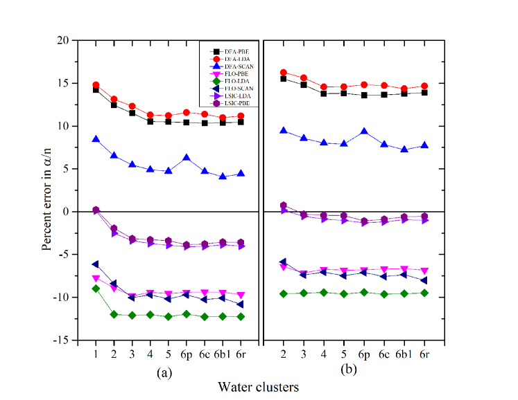
In Fig. 2 the percentage deviations of the calculated polarizabilities per molecule from the corresponding CCSD values of Ref. Hammond et al. (2009) and Alipour (2013) are plotted for all three DFAs, associated FLO-SIC-DFAs. It is interesting that the errors for LDA and PBE fall close together, lying between %, whereas the errors for SCAN range from %. For the FLO-SIC-DFA results, FLO-SIC-PBE and FLO-SIC-SCAN errors are very similar, underestimating CCSD by %, while FLO-SIC-LDA underestimates CCSD by %.
LSIC() was applied with LDA and PBE. Although gauge-consistency of the energy density in LSIC() is rigorously satisfied only for LDA, it was shown by Bhattarai et al.Bhattarai et al. (2020) that the gauge violation does not severely affect the LSIC()-PBE results. On the other hand, LSIC()-SCAN was found to be strongly affectedBhattarai et al. (2020) so we have not done LSIC()-SCAN calculations here. For polarizabilities of water clusters, we find that LSIC() shrinks the excessive correction of PZ-SIC, resulting in values that lie between the DFA and FLO-SIC-DFA results in all cases, bringing them to excellent agreement with the corresponding CCSD results. The MAE for LSIC()-LDA and LSIC()-PBE are 0.32 and 0.29 Bohr3 with respect to Ref. Hammond et al. (2009) and 0.08 and 0.06 Bohr3 with Ref. Alipour (2013). LSIC() clearly performs best among the methods employed here.
The larger 12 and 20 clusters are relatively more compact and three dimensional than the smaller clusters. They have relatively more open interior space and therefore likely to exhibit larger screening effects. It is of interest to gain some insight into whether the same relationship between DFA, PZ-SIC, and LSIC() polarizabilities continues as these effects begin to become important. Going from 6 to 12 to 20, we see a significant drop in the polarizability per molecule at the DFA, as well as the PZ-SIC and LSIC() levels due to screening. A similar drop was noted by Hammond et al. between and clustersHammond et al. (2009). It also appears that the same relationship for the values between different methods continues for the larger clusters: DFA LSIC() FLO-SIC.
We have also calculated the anisotropic polarizability for the water clusters and the values for all the functionals are presented in Table 3. CCSD values computed with the aug-cc-pVDZ basisHammond et al. (2009); Alipour (2013) are also shown. The anisotropy of polarizability of the larger clusters show an opposite trend compared to the monomer. For the monomer the DFA values are much smaller compared to CCSD values and FLO-SIC values are too large. LSIC() brings the values down closer to the reference values. For the larger clusters on the other hand DFA values are too large compared to CCSD values. The FLO-SIC values are lowered with lower MAEs. Unlike the isotropic polarizability, FLO-SIC does not degrade the performance of SCAN for the anisotropic component. LSIC() brings it even closer to the reference values. We find that the MAEs for LSIC()-LDA and LSIC()-PBE are 0.52 and 0.37 Bohr3 for the clusters up to the hexamers. At the DFA level, SCAN has the lowest MAE but at the FLO-SIC and LSIC() level PBE functional provides the best description.
| Water | DFA | FLO-SIC | LSIC() | CCSD/DZ | CCSD/TZa | CCSD/QZa | |||||
| cluster | LDA | PBE | SCAN | LDA | PBE | SCAN | LDA | PBE | . | ||
| 1 | 0.23 | 0.24 | 0.51 | 1.56 | 1.62 | 2.10 | 1.21 | 1.26 | 1.03a | 0.71 | 0.61 |
| 2 | 4.20 | 4.11 | 3.74 | 3.42 | 3.59 | 3.99 | 3.57 | 3.54 | 3.47a | 3.24 | 2.83 |
| 3 | 6.47 | 6.43 | 5.87 | 5.53 | 5.78 | 5.27 | 5.66 | 5.72 | 5.28a | 5.21 | 4.87 |
| 4 | 9.66 | 9.55 | 8.61 | 6.72 | 7.08 | 7.08 | 7.57 | 7.42 | 7.46a | 7.51 | – |
| 5 | 12.50 | 12.37 | 11.10 | 8.38 | 9.28 | 8.27 | 9.76 | 9.55 | 9.15b | – | – |
| 6p | 5.30 | 5.51 | 5.32 | 6.00 | 5.95 | 6.25 | 5.92 | 5.86 | 5.21b | – | – |
| 6c | 9.57 | 9.49 | 8.844 | 8.81 | 8.64 | 8.70 | 8.98 | 8.75 | 7.70b | – | – |
| 6b1 | 11.84 | 11.40 | 10.31 | 8.69 | 8.77 | 8.74 | 9.55 | 9.05 | 8.80b | – | – |
| 6b2 | 10.53 | 10.48 | 9.52 | 6.89 | 8.50 | 8.20 | 8.42 | 8.55 | – | – | – |
| 6r | 14.99 | 14.80 | 12.97 | 9.66 | 10.25 | 9.54 | 11.07 | 10.76 | 10.55b | – | – |
| MAE | 1.97 | 1.87 | 1.07 | 0.58 | 0.41 | 0.66 | 0.52 | 0.37 | |||
| a Reference [Hammond et al., 2009] | |||||||||||
| b Reference [Alipour, 2013] | |||||||||||
The calculated dipole moments and the polarizability of the water clusters demonstrate that the local scaling of SIC performs best among the methods employed here. As mentioned in the introduction, the polarizability depends mostly on the valence electron density which is determined by the potential in the asymptotic region. To understand further how FLO-SIC and LSIC() affect the valence electron, we compare the negative of the eigenvalues of the highest occupied orbitals with vertical ionization potentials (vIPs) calculated with CCSD(T)/aug-cc-PVTZ levels on geometries optimized at the CCSD/aug-cc-PVDZ level.Segarra-Martí et al. (2012) vIP is the transition energy between the ground state energy of a neutral system and the lowest energy of the cation that has the same geometry as the neutral system. The adiabatic IP, on the other hand, is the energy difference between the ground states of a neutral system and the cation where the cation geometry is relaxed. Segarra-Martí et al. have shown that the difference between vIP and adiabatic IP for water clusters calculated with CCSD(T) is large (2 eV).Segarra-Martí et al. (2012) Since the HOMO eigenvalues best represent the vIP without any structural relaxation, we restrict our comparison to theoretical vIP values only. These comparisons of DFA, FLO-SIC-DFA, and LSIC()-DFA are presented in Table 4. The HOMO eigenvalues at the DFA level is too high due to the incorrect asymptotic decay of the potential. FLO-SIC (PZ-SIC) corrects for that, however, it becomes too deep. The MAEs for the HOMO eigenvalues are 2.37, 1.82, and 1.97 eV for FLO-SIC-LDA, FLO-SIC-PBE, and FLO-SIC-SCAN respectively. With the LSIC() approach, the HOMO eigenvalues show excellent agreement with CCSD(T) results with MAEs of 0.40 and 0.06 eV with LDA and PBE functionals. For the sake of comparison, the self-consistent GW values from Ref. Blase et al. (2016) on the same CCSD/aug-cc-PVDZ geometries are also included. The MAE of the GW@PBE0 with respect to the CCSD(T) results is 0.35 eV, which is comparable to the LSIC()-LDA MAE. The HOMO eigenvalues show that the LSIC()-PBE describes the valence region most accurately among the methods employed here. These results are in accord with the results for polarizability where the MAE for LSIC()-PBE is found to be the smallest and the LSIC()-LDA is the second best approximation. Moreover, LSIC()-PBE values are in better agreement with CCSD(T) than GW@PBE values (MAE, 0.20 eV). This shows that the local scaling of SIC can achieve similar accuracy as more sophisticated methods. The region around the H atoms are the one-electron like regions where full SIC is applied in the LSIC() method. This is also the valence region where the SIC correction is required for good HOMO eigenvalues. Alternatively, the scaling down of SIC in the many electron region near the oxygen is necessary for a good description of polarizability and vertical ionization properties. The success of LSIC() also indicates that the selective orbital based SIC (SOSIC) methodYamamoto et al. (2020) where the SIC is applied to the selected set of orbitals (for example, HOMO) is also likely to be successful for water clusters. More applications of LSIC are necessary to determine its effectiveness for various systems and properties.
| Water | DFA | FLO-SIC | LSIC() | GW@PBEa | GW@PBE0b | CCSD(T) | |||||
| cluster | LDA | PBE | SCAN | LDA | PBE | SCAN | LDA | PBE | |||
| 1 | 7.34 | 7.20 | 7.58 | 14.72 | 14.23 | 14.26 | 12.97 | 12.64 | 12.88 | – | 12.653c |
| 2 | 6.64 | 6.49 | 6.88 | 13.98 | 13.44 | 13.59 | 12.13 | 11.79 | 12.03 | 12.15 | 11.79d |
| 3 | 7.34 | 7.15 | 7.54 | 14.62 | 14.06 | 14.23 | 12.66 | 12.29 | 12.45 | 12.60 | 12.27d |
| 4 | 7.44 | 7.25 | 7.63 | 14.68 | 14.12 | 14.28 | 12.69 | 12.32 | 12.49 | 12.63 | 12.27d |
| 5 | 7.28 | 7.09 | 7.48 | 14.53 | 13.96 | 14.14 | 12.54 | 12.17 | 12.32 | 12.47 | 12.10d |
| 6p | 6.99 | 6.80 | 7.18 | 14.22 | 13.66 | 13.82 | 12.18 | 11.81 | 11.88 | 12.04 | 11.65d |
| 6c | 7.10 | 6.91 | 7.30 | 14.34 | 13.78 | 13.94 | 12.30 | 11.93 | 12.04 | 12.18 | 11.99d |
| 6b1 | 7.03 | 6.83 | 7.22 | 14.22 | 13.62 | 13.82 | 12.17 | 11.79 | 11.91 | 12.07 | 11.69d |
| 6b2 | 7.00 | 6.81 | 7.20 | 14.20 | 13.63 | 13.30 | 12.13 | 11.76 | – | – | – |
| 6r | 7.35 | 7.15 | 7.54 | 14.58 | 14.02 | 14.19 | 12.56 | 12.19 | 12.40 | 12.54 | 12.14d |
| 12 | 7.46 | 7.25 | 7.63 | 14.63 | – | – | 12.51 | – | – | – | – |
| 20 | 7.37 | 7.16 | 7.55 | 14.56 | – | – | 12.40 | – | – | – | – |
| MAE | 4.89 | 5.08 | 4.69 | 2.37 | 1.82 | 1.97 | 0.40 | 0.06 | 0.20 | 0.35 | – |
| aGW@PBE with aug-cc-pVTZ basis from reference [Blase et al., 2016] | |||||||||||
| bGW@PBE0 with aug-cc-pVQZ and Weigend auxiliary basis from reference [Blase et al., 2016] | |||||||||||
| cReference [Blase et al., 2016] | |||||||||||
| dReference [Segarra-Martí et al., 2012] | |||||||||||
IV Summary
The effect of SIEs in the DFAs, viz. LDA, PBE-GGA, and SCAN meta-GGA functionals on the dipoles and static dipole polarizabilities of water clusters was studied using the FLO-SIC method and LSIC() methods as implemented in the FLO-SIC code. Our results show that poor description of the valence regions by DFAs results in overestimation of water cluster isotropic polarizabilities. The SCAN functional however performs relatively better than PBE or LDA with lower MAE. Incorporation of SIC results in reducing the polarizabilities however the corrected polarizability values are too small compared to the reference values. Pointwise correction with the LSIC() method brings the isotropic polarizability values with LDA and PBE closer to the reference values. Similar trends are also noticed for anisotropy in polarizability and dipole moments for which the LSIC() values are closer to the reference values compared to either DFA or FLO-SIC-DFA. The FLO-SIC (PZ-SIC) correction is on orbital by orbital basis that treats both one-electron region and many-electron regions equally. On the other hand, the LSIC() keeps the complete SIC in the one-electron like regions and scales down the correction in many-electron regions. This approach, when applied with LDA and PBE showed excellent agreement for polarizabilities with reference CCSD values. We also show that the HOMO eigenvalues of the clusters with LSIC()-LDA and LSIC()-PBE are in excellent agreement with ionization energies. The results presented here, combined with earlier applications on water cluster anions,Vargas et al. (2020) show that SIC is important for describing the electronic properties of water. This work also shows that LSIC() gives an excellent description of electronic properties of water cluster. More applications with LSIC are necessary to determine its effectiveness for other types of systems and other properties. Variations of scaling of PZ-SIC Yamamoto et al. (2020); Bhattarai et al. (2020) also need to be tested to more clearly understand the failures of PZ-SIC, which can lead to development of better functionals.
Data Availability Statement
The data that supports the findings of this study are available within the article.
Acknowledgements.
This work was supported by the US Department of Energy, Office of Science, Office of Basic Energy Sciences, as part of the Computational Chemical Sciences Program under Award No. DE-SC0018331. The work of T.B. and Y.Y. was supported in part by the US Department of Energy, Office of Science, Office of Basic Energy Sciences, under Award No. DE-SC0002168. Support for computational time at the Texas Advanced Computing Center through NSF Grant No. TG-DMR090071 and at NERSC is gratefully acknowledged.References
- Ball (2008) P. Ball, Chemical reviews 108, 74 (2008).
- Fecko et al. (2003) C. Fecko, J. Eaves, J. Loparo, A. Tokmakoff, and P. Geissler, Science 301, 1698 (2003).
- Wernet et al. (2004) P. Wernet, D. Nordlund, U. Bergmann, M. Cavalleri, M. Odelius, H. Ogasawara, L.-Å. Näslund, T. Hirsch, L. Ojamäe, P. Glatzel, et al., Science 304, 995 (2004).
- Soper and Benmore (2008) A. Soper and C. Benmore, Physical review letters 101, 065502 (2008).
- Skinner et al. (2013) L. B. Skinner, C. Huang, D. Schlesinger, L. G. Pettersson, A. Nilsson, and C. J. Benmore, The Journal of chemical physics 138, 074506 (2013).
- Pedroza et al. (2018) L. S. Pedroza, P. Brandimarte, A. R. Rocha, and M.-V. Fernández-Serra, Chemical science 9, 62 (2018).
- Elton and Fernández-Serra (2016) D. C. Elton and M. Fernández-Serra, Nature communications 7, 10193 (2016).
- Pedroza et al. (2015) L. S. Pedroza, A. Poissier, and M.-V. Fernández-Serra, The Journal of chemical physics 142, 034706 (2015).
- Piaggi and Car (2020) P. M. Piaggi and R. Car, The Journal of Chemical Physics 152, 204116 (2020).
- Sommers et al. (2020) G. M. Sommers, M. F. C. Andrade, L. Zhang, H. Wang, and R. Car, Physical Chemistry Chemical Physics 22, 10592 (2020).
- Chen et al. (2017) M. Chen, H.-Y. Ko, R. C. Remsing, M. F. Calegari Andrade, B. Santra, Z. Sun, A. Selloni, R. Car, M. L. Klein, J. P. Perdew, et al., Proceedings of the National Academy of Sciences 114, 10846 (2017), ISSN 0027-8424, eprint https://www.pnas.org/content/114/41/10846.full.pdf, URL https://www.pnas.org/content/114/41/10846.
- Santra et al. (2015) B. Santra, R. A. DiStasio Jr, F. Martelli, and R. Car, Molecular Physics 113, 2829 (2015).
- Laasonen et al. (1992) K. Laasonen, F. Csajka, and M. Parrinello, Chemical Physics Letters 194, 172 (1992), ISSN 0009-2614, URL http://www.sciencedirect.com/science/article/pii/000926149285529J.
- Laasonen et al. (1993a) K. Laasonen, M. Parrinello, R. Car, C. Lee, and D. Vanderbilt, Chemical Physics Letters 207, 208 (1993a), ISSN 0009-2614, URL http://www.sciencedirect.com/science/article/pii/000926149387016V.
- Lee et al. (1994) C. Lee, H. Chen, and G. Fitzgerald, The Journal of Chemical Physics 101, 4472 (1994), eprint https://doi.org/10.1063/1.467434, URL https://doi.org/10.1063/1.467434.
- Laasonen et al. (1993b) K. Laasonen, M. Sprik, M. Parrinello, and R. Car, The Journal of Chemical Physics 99, 9080 (1993b), eprint https://doi.org/10.1063/1.465574, URL https://doi.org/10.1063/1.465574.
- Santra et al. (2008) B. Santra, A. Michaelides, M. Fuchs, A. Tkatchenko, C. Filippi, and M. Scheffler, The Journal of Chemical Physics 129, 194111 (2008), eprint https://doi.org/10.1063/1.3012573, URL https://doi.org/10.1063/1.3012573.
- Dahlke et al. (2008) E. E. Dahlke, R. M. Olson, H. R. Leverentz, and D. G. Truhlar, The Journal of Physical Chemistry A 112, 3976 (2008), pMID: 18393474, eprint https://doi.org/10.1021/jp077376k, URL https://doi.org/10.1021/jp077376k.
- Santra et al. (2011) B. Santra, J. c. v. Klimeš, D. Alfè, A. Tkatchenko, B. Slater, A. Michaelides, R. Car, and M. Scheffler, Phys. Rev. Lett. 107, 185701 (2011), URL https://link.aps.org/doi/10.1103/PhysRevLett.107.185701.
- Asthagiri et al. (2003) D. Asthagiri, L. R. Pratt, and J. D. Kress, Phys. Rev. E 68, 041505 (2003), URL https://link.aps.org/doi/10.1103/PhysRevE.68.041505.
- Grossman et al. (2004) J. C. Grossman, E. Schwegler, E. W. Draeger, F. Gygi, and G. Galli, The Journal of Chemical Physics 120, 300 (2004), eprint https://doi.org/10.1063/1.1630560, URL https://doi.org/10.1063/1.1630560.
- Schwegler et al. (2004) E. Schwegler, J. C. Grossman, F. Gygi, and G. Galli, The Journal of Chemical Physics 121, 5400 (2004), eprint https://doi.org/10.1063/1.1782074, URL https://doi.org/10.1063/1.1782074.
- Gillan et al. (2016) M. J. Gillan, D. AlfÚ, and A. Michaelides, The Journal of Chemical Physics 144, 130901 (2016), eprint https://doi.org/10.1063/1.4944633, URL https://doi.org/10.1063/1.4944633.
- Sun et al. (2015) J. Sun, A. Ruzsinszky, and J. P. Perdew, Phys. Rev. Lett. 115, 036402 (2015), URL https://link.aps.org/doi/10.1103/PhysRevLett.115.036402.
- Sun et al. (2016) J. Sun, R. C. Remsing, Y. Zhang, Z. Sun, A. Ruzsinszky, H. Peng, Z. Yang, A. Paul, U. Waghmare, X. Wu, et al., Nature Chemistry 8, 831 (2016), ISSN 1755-4349, URL https://doi.org/10.1038/nchem.2535.
- Miliordos et al. (2013) E. Miliordos, E. Aprà, and S. S. Xantheas, The Journal of Chemical Physics 139, 114302 (2013), eprint https://doi.org/10.1063/1.4820448, URL https://doi.org/10.1063/1.4820448.
- Sharkas et al. (2020) K. Sharkas, K. Wagle, B. Santra, S. Akter, R. R. Zope, T. Baruah, K. A. Jackson, J. P. Perdew, and J. E. Peralta, Proc. Natl. Acad. Sci. (2020), to appear.
- Jensen et al. (2002) L. Jensen, M. Swart, P. T. van Duijnen, and J. G. Snijders, The Journal of Chemical Physics 117, 3316 (2002), eprint https://doi.org/10.1063/1.1494418, URL https://doi.org/10.1063/1.1494418.
- Tu and Laaksonen (2000) Y. Tu and A. Laaksonen, Chemical Physics Letters 329, 283 (2000), ISSN 0009-2614, URL http://www.sciencedirect.com/science/article/pii/S0009261400010265.
- Ghanty and Ghosh (2003) T. K. Ghanty and S. K. Ghosh, The Journal of Chemical Physics 118, 8547 (2003), eprint https://doi.org/10.1063/1.1573171, URL https://doi.org/10.1063/1.1573171.
- Yang et al. (2005) M. Yang, P. Senet, and C. Van Alsenoy, International Journal of Quantum Chemistry 101, 535 (2005), eprint https://onlinelibrary.wiley.com/doi/pdf/10.1002/qua.20308, URL https://onlinelibrary.wiley.com/doi/abs/10.1002/qua.20308.
- Yang et al. (2010) F. Yang, X. Wang, M. Yang, A. Krishtal, C. van Alsenoy, P. Delarue, and P. Senet, Phys. Chem. Chem. Phys. 12, 9239 (2010), URL http://dx.doi.org/10.1039/C001007C.
- Krishtal et al. (2006) A. Krishtal, P. Senet, M. Yang, and C. Van Alsenoy, The Journal of Chemical Physics 125, 034312 (2006), eprint https://doi.org/10.1063/1.2210937, URL https://doi.org/10.1063/1.2210937.
- Medders and Paesani (2013) G. R. Medders and F. Paesani, Journal of Chemical Theory and Computation 9, 4844 (2013), pMID: 26583403, eprint https://doi.org/10.1021/ct400696d, URL https://doi.org/10.1021/ct400696d.
- Hammond et al. (2009) J. R. Hammond, N. Govind, K. Kowalski, J. Autschbach, and S. S. Xantheas, The Journal of Chemical Physics 131, 214103 (2009), eprint https://doi.org/10.1063/1.3263604, URL https://doi.org/10.1063/1.3263604.
- Xantheas (1996) S. S. Xantheas, The Journal of Chemical Physics 104, 8821 (1996), eprint https://doi.org/10.1063/1.471605, URL https://doi.org/10.1063/1.471605.
- Xantheas et al. (2002) S. S. Xantheas, C. J. Burnham, and R. J. Harrison, The Journal of Chemical Physics 116, 1493 (2002), eprint https://doi.org/10.1063/1.1423941, URL https://doi.org/10.1063/1.1423941.
- Alipour (2013) M. Alipour, The Journal of Physical Chemistry A 117, 4506 (2013).
- Alipour and Fallahzadeh (2017) M. Alipour and P. Fallahzadeh, Theoretical Chemistry Accounts 136, 22 (2017), ISSN 1432-2234, URL https://doi.org/10.1007/s00214-016-2046-y.
- Jackson et al. (2019) K. A. Jackson, J. E. Peralta, R. P. Joshi, K. P. Withanage, K. Trepte, K. Sharkas, and A. I. Johnson, Journal of Physics: Conference Series 1290, 012002 (2019), URL https://doi.org/10.1088%2F1742-6596%2F1290%2F1%2F012002.
- Vargas et al. (2020) J. Vargas, P. Ufondu, T. Baruah, Y. Yamamoto, K. A. Jackson, and R. R. Zope, Phys. Chem. Chem. Phys. 22, 3789 (2020), URL http://dx.doi.org/10.1039/C9CP06106A.
- Withanage et al. (2019) K. P. K. Withanage, S. Akter, C. Shahi, R. P. Joshi, C. Diaz, Y. Yamamoto, R. Zope, T. Baruah, J. P. Perdew, J. E. Peralta, et al., Phys. Rev. A 100, 012505 (2019), URL https://link.aps.org/doi/10.1103/PhysRevA.100.012505.
- Perdew and Schmidt (2001) J. P. Perdew and K. Schmidt, AIP Conference Proceedings 577, 1 (2001), eprint https://aip.scitation.org/doi/pdf/10.1063/1.1390175, URL https://aip.scitation.org/doi/abs/10.1063/1.1390175.
- Perdew et al. (1996) J. P. Perdew, K. Burke, and M. Ernzerhof, Phys. Rev. Lett. 77, 3865 (1996), URL https://link.aps.org/doi/10.1103/PhysRevLett.77.3865.
- Zope et al. (2019) R. R. Zope, Y. Yamamoto, C. M. Diaz, T. Baruah, J. E. Peralta, K. A. Jackson, B. Santra, and J. P. Perdew, The Journal of Chemical Physics 151, 214108 (2019), eprint https://doi.org/10.1063/1.5129533, URL https://doi.org/10.1063/1.5129533.
- Pederson et al. (2014) M. R. Pederson, A. Ruzsinszky, and J. P. Perdew, The Journal of Chemical Physics 140, 121103 (2014), eprint https://doi.org/10.1063/1.4869581, URL https://doi.org/10.1063/1.4869581.
- Pederson (2015) M. R. Pederson, The Journal of Chemical Physics 142, 064112 (2015), eprint https://doi.org/10.1063/1.4907592, URL https://doi.org/10.1063/1.4907592.
- Yang et al. (2017) Z.-h. Yang, M. R. Pederson, and J. P. Perdew, Phys. Rev. A 95, 052505 (2017), URL https://link.aps.org/doi/10.1103/PhysRevA.95.052505.
- Pederson and Baruah (2015) M. R. Pederson and T. Baruah, in Advances In Atomic, Molecular, and Optical Physics, edited by E. Arimondo, C. C. Lin, and S. F. Yelin (Academic Press, 2015), vol. 64 of Advances In Atomic, Molecular, and Optical Physics, pp. 153 – 180, URL http://www.sciencedirect.com/science/article/pii/S1049250X15000087.
- (50) R. R. Zope, T. Baruah, and K. A. Jackson, FLOSIC 0.2, based on the NRLMOL code of M. R. Pederson, URL https://http://flosic.org/.
- Porezag and Pederson (1999) D. Porezag and M. R. Pederson, Phys. Rev. A 60, 2840 (1999), URL https://link.aps.org/doi/10.1103/PhysRevA.60.2840.
- Pederson and Jackson (1990) M. R. Pederson and K. A. Jackson, Phys. Rev. B 41, 7453 (1990), URL https://link.aps.org/doi/10.1103/PhysRevB.41.7453.
- Löwdin (1950) P.-O. Löwdin, The Journal of Chemical Physics 18, 365 (1950).
- Pederson et al. (1984) M. R. Pederson, R. A. Heaton, and C. C. Lin, J. Comp. Phys. 80, 1972 (1984), eprint https://doi.org/10.1063/1.446959, URL https://doi.org/10.1063/1.446959.
- Pederson et al. (1985) M. R. Pederson, R. A. Heaton, and C. C. Lin, J. Comp. Phys. 82, 2688 (1985), eprint https://doi.org/10.1063/1.448266, URL https://doi.org/10.1063/1.448266.
- Yamamoto et al. (2020) Y. Yamamoto, S. Romero, T. Baruah, and R. R. Zope, The Journal of Chemical Physics 152, 174112 (2020), eprint https://doi.org/10.1063/5.0004738, URL https://doi.org/10.1063/5.0004738.
- Van Leeuwen and Baerends (1994) R. Van Leeuwen and E. Baerends, Physical Review A 49, 2421 (1994).
- Van Gisbergen et al. (2001) S. Van Gisbergen, J. Pacheco, and E. Baerends, Physical Review A 63, 063201 (2001).
- Grüning et al. (2002) M. Grüning, O. V. Gritsenko, S. J. Van Gisbergen, and E. Jan Baerends, The Journal of chemical physics 116, 9591 (2002).
- Banerjee et al. (2007) A. Banerjee, A. Chakrabarti, and T. K. Ghanty, The Journal of chemical physics 127, 134103 (2007).
- Banerjee et al. (2008) A. Banerjee, T. K. Ghanty, and A. Chakrabarti, The Journal of Physical Chemistry A 112, 12303 (2008).
- Schipper et al. (2000) P. R. Schipper, O. V. Gritsenko, S. J. van Gisbergen, and E. J. Baerends, The Journal of Chemical Physics 112, 1344 (2000).
- Zope et al. (2008) R. R. Zope, T. Baruah, M. R. Pederson, and B. I. Dunlap, International Journal of Quantum Chemistry 108, 307 (2008), eprint https://onlinelibrary.wiley.com/doi/pdf/10.1002/qua.21458, URL https://onlinelibrary.wiley.com/doi/abs/10.1002/qua.21458.
- Schwalbe et al. (2018) S. Schwalbe, T. Hahn, S. Liebing, K. Trepte, and J. Kortus, Journal of Computational Chemistry 39, 2463 (2018), eprint https://doi.org/10.1002/jcc.25586.
- Perdew and Wang (1992) J. P. Perdew and Y. Wang, Phys. Rev. B 45, 13244 (1992), URL https://link.aps.org/doi/10.1103/PhysRevB.45.13244.
- Yamamoto et al. (2019) Y. Yamamoto, C. M. Diaz, L. Basurto, K. A. Jackson, T. Baruah, and R. R. Zope, The Journal of chemical physics 151, 154105 (2019).
- Rakshit et al. (2019) A. Rakshit, P. Bandyopadhyay, J. P. Heindel, and S. S. Xantheas, The Journal of Chemical Physics 151, 214307 (2019), eprint https://doi.org/10.1063/1.5128378, URL https://doi.org/10.1063/1.5128378.
- Gregory et al. (1997) J. Gregory, D. Clary, K. Liu, M. Brown, and R. Saykally, Science 275, 814 (1997).
- Johnson et al. (2019) A. I. Johnson, K. P. K. Withanage, K. Sharkas, Y. Yamamoto, T. Baruah, R. R. Zope, J. E. Peralta, and K. A. Jackson, The Journal of Chemical Physics 151, 174106 (2019), eprint https://doi.org/10.1063/1.5125205, URL https://doi.org/10.1063/1.5125205.
- Lovas (1978) F. J. Lovas, Journal of Physical and Chemical Reference Data 7, 1445 (1978), eprint https://doi.org/10.1063/1.555588, URL https://doi.org/10.1063/1.555588.
- Dyke et al. (1977) T. R. Dyke, K. M. Mack, and J. S. Muenter, The Journal of Chemical Physics 66, 498 (1977), eprint https://doi.org/10.1063/1.433969, URL https://doi.org/10.1063/1.433969.
- Zeiss and Meath (1975) G. Zeiss and W. J. Meath, Molecular Physics 30, 161 (1975), eprint https://doi.org/10.1080/00268977500101841, URL https://doi.org/10.1080/00268977500101841.
- Murphy (1977) W. F. Murphy, The Journal of Chemical Physics 67, 5877 (1977), eprint https://doi.org/10.1063/1.434794, URL https://doi.org/10.1063/1.434794.
- Pederson et al. (2005) M. R. Pederson, T. Baruah, P. B. Allen, and C. Schmidt, Journal of Chemical Theory and Computation 1, 590 (2005), ISSN 1549-9618, URL https://doi.org/10.1021/ct050061t.
- Bhattarai et al. (2020) P. Bhattarai, K. Wagle, C. Shahi, Y. Yamamoto, S. Romero, B. Santra, R. R. Zope, J. E. Peralta, K. A. Jackson, and J. P. Perdew, The Journal of Chemical Physics 152, 214109 (2020), eprint https://doi.org/10.1063/5.0010375, URL https://doi.org/10.1063/5.0010375.
- Segarra-Martí et al. (2012) J. Segarra-Martí, M. Merchán, and D. Roca-Sanjuán, The Journal of Chemical Physics 136, 244306 (2012), eprint https://doi.org/10.1063/1.4730301, URL https://doi.org/10.1063/1.4730301.
- Blase et al. (2016) X. Blase, P. Boulanger, F. Bruneval, M. Fernandez-Serra, and I. Duchemin, The Journal of Chemical Physics 144, 034109 (2016), eprint https://doi.org/10.1063/1.4940139, URL https://doi.org/10.1063/1.4940139.