Pairbot: A Novel Model for Autonomous Mobile Robot Systems Consisting of Paired Robots

Abstract

Programmable matter consists of many self-organizing computational entities which are autonomous and cooperative with one another to achieve a goal and it has been widely studied in various fields, e.g., robotics or mobile agents, theoretically and practically. In the field of computer science, programmable matter can be theoretically modeled as a distributed system consisting of simple and small robots equipped with limited capabilities, e.g., no memory and/or no geometrical coordination. A lot of theoretical research is studied based on such theoretical models, to clarify the relation between the solvability of various problems and the considered models.

We newly propose a computational model named Pairbot model where two autonomous mobile robots operate as a pair on a grid plane. In Pairbot model, every robot has the one robot as its unique partner, called buddy, each other. We call the paired two robots pairbot. Two robots in one pairbot can recognize each other, and repeatedly change their geometrical relationships, long and short, to achieve the goal.

In this paper, as a first step to show the feasibility and effectiveness of the proposed Pairbot model, we introduce two simple problems, the marching problem and the object coating problem, and propose two algorithms to solve these two problems, respectively. In both algorithms, it is assumed that the visibility range is one (every robot can observe only its neighboring robots) and the scheduler is asynchronous (ASYNC).

Keywords Autonomous robots  $\cdot$ Distributed coordination  $\cdot$ Programmable matter  $\cdot$ LCM model  $\cdot$ Triangular grid

1 Introduction

1.1 Background

The seminal paper [1] firstly introduced a concept of a distributed system consisting of multiple mobile robots, where each robot autonomously observes the positions of the other robots and moves to a new position based on the given algorithm. The robots are anonymous, i.e., cannot be distinguished by their appearance, and uniform, i.e., execute the same algorithm. In the literature [1], they call the mobile robot model LCM(Look-Compute-Move)-model, and give a formal discussion on the power and limitations of the distributed coordination, e.g., pattern formation and agreement problems. Since the introduction of LCM-model, much related work has been studied to clarify its computational power and limitations [2, 3] for over twenty years.

As one simple problem in LCM-model, a gathering problem for two robots, called a rendezvous problem is widely studied in the literature as [4, 5]. The gathering problems for more than two robots are also investigated in much of literature such as [6, 7, 8, 9, 10]. Not only the gathering problems, but many other distributed coordination problems are also studied from the viewpoint of the relation between the computational capabilities and the solvability of the problems. The pattern formation problem [11, 12, 13] is also one of the fundamental coordination problems which makes the robots to form the given pattern, e.g., line or circle. The pattern formation problem is practically important because if the robots can form the given pattern, they can agree on some specific roles, e.g., a leader, a center, or a corner. In a wide sense, the gathering problem can be also categorized as the one of the pattern formation (forming a point).

Many of studies mainly focus on the relation between the computational capabilities of each robot and the solvability of the given problem. This means that the clarification of the required (possibly minimum) capabilities to solve the given problem is an important issue. To solve the given problem, many capabilities of each robot should be considered, e.g., geometric agreement, scheduler, visibility, transparency, and many others, and many results show that the solvability of each problem deeply depends on these capabilities. To clarify the required capabilities for the given problem has many advantages [3], for example, reducing the costs, making easy to expand of the system (scalability), and allowing fault-tolerance. Therefore, various distributed coordination problems for autonomous mobile robots are still widely studied in many fields, such as robotics, engineering, or medical science.

1.2 Related Work

Based on the seminal work [1] which firstly introduced an autonomous mobile robot model and its computational capability, much related work has been investigated about discussing its computational power and limitations for various distributed coordination [2, 3], e.g., rendezvous[14, 4, 5, 15, 16], gathering[17, 7, 8, 9, 10, 18], pattern formations[13, 19, 12, 11, 20, 21], and flocking[22, 23, 24].

As an extended capability of mobile robots, an externally visible memory register, called light, is proposed in [25]. An autonomous mobile robot with the light is called a luminous robot, and every luminous robot maintains a persistent value, called color, which means that the value is never reset even if an oblivious robot terminates its action. Each luminous robot can observe the colors of the other robots within its visibility range, and this improves the power of each mobile robot, hence, many problems are newly investigated based on this capability such as [26, 27, 15, 16, 28].

Recently, a programming matter[29], which is a matter that can change its physical properties, e.g., shape or density, in a programmable fashion, and it attracts much attention of many researchers as one of the practical applications of distributed coordination, e.g., the realization of surgical treatments using nanorobots [30] or a set of modular robots which can freely transform its shape[31, 32]. As the one method to realize a programming matter, a self-organizing particle system, also called Amoebot model, is newly proposed in [33]. Amoebot model consists of a large number of computational particles on a (triangular) grid plane which locally interacts one another to solve the given problem. Each particle repeatedly changes its state, either contraction or expansion, which means the state that a particle occupies one node and two adjacent nodes respectively. In Amoebot model, it allows two connected particles to perform a coordinated movement, called a handover, which is an interaction that a particle can contract out of a certain node at the same time as another particle expand into that node. Amoebot model can realize many distributed coordination problems such as a universal coating problem[34], a leader election[35], convex hull formation[36], and many others.

Amoebot model has some imperative differences from the conventional autonomous mobile robots [1]. In Amoebot model, each particle can communicate by writing their local memory and reading the local memory of adjacent particles, whereas there is no explicit communication in autonomous mobile robots (known as LCM-model). In LCM-model, each robot determines its behavior based on the snapshot taken at Look phase instead of a communication. Moreover, Amoebot model assumes the symmetry breaking: when two or more particles attempt to move to the same cell, one of them will succeed. On the other hand, each robot in autonomous mobile robots cannot break the symmetry when two or more robots attempt to move the same point, which implies that a sophisticate algorithm is required to avoid some unintended movement among the robots.

1.3 Contribution

In this paper, we consider a new method for realizing a programmable matter that makes it easy to investigate and analyze its capabilities and feasibilities by using existing knowledge. We introduce a new model named Pairbot model where two robots operate as a pair on a grid plane. Pairbot model has several new capabilities, e.g., local label or exclusive move, which are not assumed in a classical LCM-model, but most of capabilities are the same as LCM-model’s. The new capabilities provide higher computational power (i.e., solvability) than LCM-model, as well as good insight for realization of programmable matter based on LCM-model.

Amoebot model [33] is another new model for programmable matter which is inspired by the behavior of amoeba. Amoebot model has new computational capabilities, e.g., communication, symmetry breaking, and occupying two points, which are not assumed in the conventional LCM-model. Therefore, it is difficult to directly compare the computational capability between Amoebot model and LCM-model. On the other hand, Pairbot model is a new theoretical model which has many same capabilities as LCM-model’s, thus the differences between Pairbot model and LCM-model are also clear. By the similarity and difference between Pairbot model and LCM-model, Pairbot model provides higher computational power than LCM-model, moreover, it is also possible to introduce plenty of knowledge from many results about LCM-model investigated over twenty years.

In the proposed model, Pairbot model, each robot has the one robot as its unique partner, called buddy, each other, and we call the paired two robots pairbot. A pairbot system consists of two or more pairbot. Each of two robots in one pairbot can recognize each other as its buddy, and the two robots repeatedly change their geometrical relationship, short and long, to achieve a goal. When a pairbot is in short state, the two robots occupy the same point, whereas in long state, the two robots are located on the two distinct (adjacent) points.

As the first step to show the feasibility and effectiveness of Pairbot model, we introduce two simple problems, the marching problem and the object coating problem, and propose two deterministic algorithms to solve these two problems respectively. We expect that these two problems and algorithms help to understand Pairbot model, and provide a good insight for its computational power and limitations.

1.4 Paper Organization

This paper is organized as follows: Section 2 introduces the proposed system model named Pairbot model. Section 3 gives the marching problem based on Pairbot model, and proposes an algorithm to solve the marching problem, and we present another problem named the object coating problem and the algorithm to solve the problem in Section 4. We conclude our work in Section 5.

2 The Proposed Model: Pairbot model

2.1 Triangular Grid Plane

Figure 1: Triangular grid plane $\mathbb{T}$

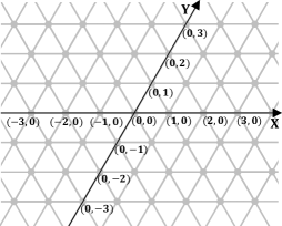
We consider a set of $n$ autonomous mobile robots, denoted by $\mathscr{R}=\{r_{1},r_{2},\ldots,r_{n}\}$ on a 2-dimensional triangular grid plane $\mathbb{T}=\mathbf{Z}^{2}$ like Fig.1. The distance between two points $u$ and $v$ on $\mathbb{T}$ is defined by the following equation.

$$\mathit{dist}(u,v)=\left\{\begin{array}[]{l}|u.x-v.x|+|u.y-v.y|\hskip 10.0pt\mathit{\bf if}~{}(u_{x}-v_{x})(u_{y}-v_{y})\geq 0\\ |u.x-v.x|+|u.y-v.y|-\mathit{min}(|u.x-v.x|,|u.y-v.y|)\hskip 10.0pt\mathit{\bf otherwise}\\ \end{array}\right.$$ (3)

If the distance between two points is one, we say that the two points are adjacent. The triangular grid plane $\mathbb{T}$ can be also represented as an infinite regular graph $G_{\mathbb{T}}=(V_{\mathbb{T}},E_{\mathbb{T}})$, where $V_{\mathbb{T}}$ consists of all the points on $\mathbb{T}$ and $E_{\mathbb{T}}$ is defined by every two adjacent points on $\mathbb{T}$, i.e., for $u$, $v\in V_{\mathbb{T}}$, $(u,v)\in E_{\mathbb{T}}$ iff $\mathit{dist}(u,v)=1$.

2.2 Geometric Agreement

Every robot has its own local coordinate system which can be defined by the directions, i.e., $X$ and $Y$ axes, and the orientations, i.e., the positive and negative side of each axis. We can consider some levels of consistency among the robots on their local compass: total agreement, when all the robots agree on the directions and orientations of both axes; partial agreement, when all the robots agree on the direction and orientation of only one axis or they agree on chirality which means a sense of the orientation of the axes, i.e., clockwise or counter-clockwise; or no agreement, when there is no agreement among the local coordinate system of each robot.

In this paper, we assume total agreement that all the robots in $\mathscr{R}$ agree on the directions and orientations of both axes, but no robot knows the position of the origin. In other words, no robot knows its global coordinate, however, all the robots agree on the sense of directions, e.g., north, south, east, and west.

2.3 Pairbot

In Pairbot model, every robot has its unique partner (called buddy): robot $r_{i}$ is the buddy of robot $r_{j}$ if and only if robot $r_{j}$ is the buddy of robot $r_{i}$. When robots $r_{i}$ and $r_{j}$ are determined as a pair, we call the two robots $r_{i}$ and $r_{j}$ a pairbot, and denote as $\mathit{pair}(r_{i},r_{j})$.

The buddy of each robot is initially determined and never changes. Obviously, the number of robots $n$ is an even number because every robot has its corresponding buddy, and without loss of generality, we assume that robots $r_{i}$ and $r_{i+1}$ are the pairbot for an odd number $i$, i.e., $\mathit{pair}(r_{i},r_{i+1})$, where $\forall r_{i}\in\mathscr{R}~{}|~{}i=2k+1~{}(0\leq k\leq(n/2-1))$.

Operations

Each robot $r_{i}$ cyclically performs the following three operations, Look, Compute, and Move, based on a well-known computational model as LCM-model or Suzuki-Yamashita model [1].

• Look: Each robot takes a snapshot consisting of the robots within the visibility range with respect to its local coordinate system.

• Compute: Each robot performs a local computation based on the snapshot taken by Look phase according to algorithm $\mathscr{A}$. Algorithm $\mathscr{A}$ is basically uniform, i.e., every robot executes the same algorithm. As the result of Compute phase, each robot determines its destination point to move.

• Move: Based on the result of Compute phase, each robot actually moves to the adjacent destination point from the current point in Move phase. Each robot moves instantly, this implies that each robot is never looked by the other robots while moving. Null movement (staying) is also allowed, i.e., a robot does not move.

Local Label

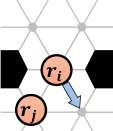
Each robot locally maintains the labels for each incident edge, from 1 to 6, to distinguish its adjacent points. Each robot selects one incident edge, labels the selected edge as 1, and labels the other edges from 2 to 6 in clockwise order. Note that the direction of the edge labeled as 1 may be different by the assumption of the geometric agreements among robots, moreover, the clockwise order may also vary by the assumption of chirality.

Figure 2: An example of Local labels of each robot without any geometric agreement

Fig.2 represents an example of local labels of each robot where there is no agreement among robots. In Fig.2, robot $r_{i}$ labels the edge on the right side as 1, however, robot $r_{j}$ or $r_{k}$ labels the edge which has different direction with $r_{i}$’s as 1. This is because the robots do not agree on the directions and orientation of any axis. Moreover, the edges of robot $r_{k}$ are labeled in counter-clockwise order, because the robots do not agree on chirality.

In this paper, every robot has the same local labels, e.g., every robot maintains the same labels as robot $r_{i}$ in Fig.2 due to total agreement.

Capabilities

All the robots are oblivious, i.e., no memory, which means every robot never knows any past executions of itself.

Each robot can recognize the other robots within its visibility range $\mathscr{V}$, this means each robot can sense only up to $\mathscr{V}$ hops far from itself. In other words, robot $r_{u}$ on point $u$ and robot $r_{v}$ on point $v$ (where $r_{u},r_{v}\in\mathscr{R}$ and $u,v\in V_{\mathbb{T}}$) can observe each other only when $\mathit{dist}(u,v)\leq\mathscr{V}$. In this paper, we assume that the visibility range of each robot is one, i.e., each robot can observe only the robots at the adjacent points.

Moreover, we assume that each robot has capability of weak multiplicity detection, that is, each robot can distinguish from the following three cases on the points within its visibility, no robot exists, only one robot exists, and more than one robot exists. Note that if each robot can count the exact number of the robots occupying the point within its visibility range, we say it strong multiplicity detection.

All the robots in $\mathscr{R}$ are anonymous: each robot has no identifier and no robot is distinguishable by its appearance. However, each robot maintains the position of its buddy using its local label. This implies that each robot has a local memory to maintain the position (local label) where its buddy is located.

Moreover, we assume that when a pairbot occupies the same point, only one robot can move to its adjacent point when it moves and we call this an exclusive move. Note that no robot knows that any other two robots are pairbot or not.

(a) short state

(b) long state

Figure 3: Two states of pairbot

Figure 4: An example of pairbots

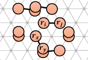
The two robots in one pairbot occupy the same point or two adjacent points on $\mathbb{T}$ as Fig.4. We call the former one short state and the latter one long state respectively. When a pairbot is in short state, only one robot in the pairbot can (exclusively) move the adjacent point from its current point and the pairbot becomes long state. When a pairbot is in long state, either of the two robots can move to the point occupied by its buddy, and the state is changed back to short state. In Pairbot model, every pairbot repeatedly changes its state, short and long, to achieve the goal. Obviously, a pairbot never knows which robot moved while its state changed because all the robots are oblivious.

Fig.4 illustrates an example of pairbots. pairbot, $r_{i}$ and $r_{j}$, is in long state, and some other robots are placed on the other points on $\mathbb{T}$. In this case, robot $r_{i}$ recognizes that its buddy is robot $r_{j}$ on its right side. However, $r_{i}$ cannot know the pair relations of the other robots, e.g., robot $r_{i}$ never knows the buddy of robot $r_{x}$ on its lower left side. Robot $r_{y}$ can recognize another robot is on the same point due to weak multiplicity detection, moreover, $r_{y}$ can know that the buddy $r_{x}$ is on the point of its upper left side and it is in long state.

2.4 Scheduler

We consider a scheduler which decides which robot to activate and the timing of each operation. There are three representative assumptions (models) for a scheduler, fully-synchronous (FSYNC), semi-synchronous (SSYNC), and asynchronous (ASYNC).

In an FSYNC scheduler, all the robots are activated at the same time and all the three operations, Look, Compute, and Move, are executed based on the exactly same cycle time. In an SSYNC scheduler, all the robots execute their operations at the same time, but some robots may not be activated. The robots which are not activated by a scheduler wait till all the activated robots terminate their operations. And in an ASYNC scheduler, there is no assumption on the cycle time of each robot. This implies that all the robots execute their operations at unpredictable time instants and durations.

In this paper, we assume an ASYNC scheduler such that Move phase operates atomically: each robot requires unpredictable finite time to operate Look or Compute phase, but it can atomically move, called the move-atomic property. Therefore, each robot is never observed while it is moving. We assume that the two robots which are the pairbot are activated at the same time by the scheduler.

2.5 Configuration

A configuration $\mathscr{C}_{t}$ consists of the positions of all the robots in $\mathscr{R}$ at time $t$: $\mathscr{C}_{t}=\{(r_{1}.x(t),r_{1}.y(t)),(r_{2}.x(t),r_{2}.y(t)),\ldots,(r_{n}.x(t),r_{n}.y(t))\}$, where $(r_{i}.x(t),r_{i}.y(t))$ is the global coordinate of robot $r_{i}$ at time $t$ on $\mathbb{T}$. Note that no robot knows its global coordinate on $\mathbb{T}$. Let $\mathscr{R}^{\prime}$ be a non-empty subset of $\mathscr{R}$ and $\mathscr{A}$ be an algorithm, we denote $\mathscr{C}_{t}\mapsto_{(\mathscr{R}^{\prime},\mathscr{A})}\mathscr{C}_{t+1}$ if a configuration $\mathscr{C}_{t+1}$ is obtained when each robot in $\mathscr{R}^{\prime}$ simultaneously performs its Move operation of $\mathscr{A}$ in configuration $\mathscr{C}_{t}$. Hence a scheduler can be presented as an infinite sequence $\mathscr{R}_{1},\mathscr{R}_{2},\cdots$ of non-empty subsets of $\mathscr{R}$. An execution $\Xi_{\mathscr{A}}(\mathscr{S},\mathscr{C}_{0})$ of algorithm $\mathscr{A}$ along schedule $\mathscr{S}=\mathscr{R}_{1},\mathscr{R}_{2},\cdots$ starting from configuration $\mathscr{C}_{0}$, where $\mathscr{C}_{0}$ is an initial configuration, can be defined as the infinite sequence of configurations $\mathscr{C}_{0},\mathscr{C}_{1},\cdots$ such that $\mathscr{C}_{i}\mapsto_{(\mathscr{R}_{i+1},\mathscr{A})}\mathscr{C}_{i+1}$ for all $i\geq 0$.

3 Marching Problem and Algorithm

In this section, we introduce a basic problem, named the marching problem, for Pairbot model, and propose an algorithm to solve the marching problem.

3.1 Problem Definition

We consider a marching, which is a linear movement of the robots lined up in a straight line to the agreed direction keeping their line formation, as a basic moving operation of the set of pairbots. Before the formal definition of the marching problem, we define a specific formation of the pairbots.

We consider that the set of robots $\mathscr{R}$ initially forms a straight line as Fig.5, i.e., if any two points are occupied by robots, every point located between the two points is occupied by a robot. We assume that the straight line formed by the robots is parallel to the agreed direction. And we also assume that there are at most two robots on each point, however, there exist no two pairbots which are in long state on the two same points. For example, let robots $r_{a}$ and $r_{b}$ be one pairbot and robots $r_{c}$ and $r_{d}$ be another pairbot. In this case, we do not consider the configuration such that $r_{a}$ and $r_{c}$ occupy the same point and $r_{b}$ and $r_{d}$ occupy another same point (which is an adjacent to the point occupied by $r_{a}$ and $r_{c}$). We call above configuration the robots (pairbots) are line-formed.

Figure 5: An example configuration that the pairbots form a straight line

Now we define the marching problem as the following.

Definition 1

Marching (Linear Movement) Problem. The pairbots are initially line-formed, and let $r_{h}$ be the robot where there is no robot on the side of the direction to move, e.g., $r_{h}$ is the rightmost robot if the direction to move is right. Algorithm $\mathscr{A}$ solves the marching problem if any execution satisfies the following conditions:

• The robots are line-formed.

• Robot $r_{h}$ moves to its adjacent unoccupied point on the side of the directions to move within the finite number of executions.

Intuitively, in the marching problem, all the robots repeatedly move to the agreed direction keeping line-formed. And the termination is not considered in the marching problem.

3.2 Marching Algorithm

To help to understand, in this subsection, we assume that the positive direction of $X$ axis is on the right side like Fig.1. Note that all the robots agree on the direction and orientation of one axis, thus we can assume that every robot labels the edge on its right side as 1 (refer to robot $r_{i}$ in Fig.2).

We describe the proposed algorithm using guarded actions: $<guard>\Rightarrow<action>$, which represents $<action>$ is executed only if $<guard>$ becomes true.

Algorithm 1 Marching Algorithm for robot $r_{i}$

assumption: The set of robots is line-formed on the line parallel to $X$ axis.

variables and functions:

$~{}\cdot~{}\ell_{x}$ :

The adjacent point to the edge labeled $x$ ($x\in\{1,\ldots,6\}$). As an exception, $\ell_{0}$ means the current point occupied by $r_{i}$.

$~{}\cdot~{}\mathit{buddy}$ :

The point where its buddy occupies. If the pairbot is in long state, $\mathit{buddy}$ becomes one among $\ell_{1}$ to $\ell_{6}$, but $\ell_{0}$ otherwise (short state).

$~{}\cdot~{}\mathit{occupy}(\ell_{x})$ :

A function returns the number of robots on the point $\ell_{x}$. Function $\mathit{occupy}(\ell_{x})$ returns $2$ even if there are $2$ or more robots on the point $\ell_{x}$ because we assume weak multiplicity detection, thus, $\mathit{occupy}(\ell_{x})\in\{0,1,2\}$.

algorithm:

1:$(\mathit{buddy}=\ell_{0})\wedge(\mathit{occupy}(\ell_{1})<2)\Rightarrow$ Exclusive move to $\ell_{1}$

2:$(\mathit{buddy}=\ell_{1})\wedge(\mathit{occupy}(\ell_{1})=1)\wedge(\mathit{occupy}(\ell_{4})=0)\Rightarrow$ Move to $\ell_{1}$

3:$(\mathit{buddy}=\ell_{1})\wedge(\mathit{occupy}(\ell_{1})=1)\wedge(\mathit{occupy}(\ell_{0})=2)\Rightarrow$ Move to $\ell_{1}$

Algorithm 1 represents the marching algorithm where the move to the direction is $\ell_{1}$. In Algorithm 1, line 1 can be executed only when a pairbot is in short state, and line 2 or line 3 can be executed only when a pairbot is in long state. To help to explain, we call the robot which has no neighboring robot on $\ell_{1}$ the head robot (denote $r_{h}$), i.e., $r_{h}.\mathit{occupy}(\ell_{1})=0$, and call the robot which has no neighboring robot on $\ell_{4}$ (the counter direction of $\ell_{1}$) the tail robot (denote $r_{t}$), i.e., $r_{t}.\mathit{occupy}(\ell_{4})=0$. Note that there can be two head robots (and/or tail robots) when the pairbot is in short state.

A pairbot in short state, i.e., $\mathit{buddy}=\ell_{0}$, checks the adjacent point $\ell_{1}$, and it becomes long state by an exclusive move of one robot to the point $\ell_{1}$ if one or no robot is on $\ell_{1}$. Obviously, the head robot always moves to $\ell_{1}$ and becomes long state when it is in short state.

If the pairbots are in long state, the tail-sided robot of the two robots, i.e., a robot which has its buddy on $\ell_{1}$, moves toward its buddy (on $\ell_{1}$) when either of the two conditions (lines 2 and 3) is satisfied. Let $r_{i}$ be a robot which has its buddy on $\ell_{1}$, i.e., $\mathit{buddy}=\ell_{1}$ (long state). If there is no robot on $r_{i}.\ell_{4}$, which means $r_{i}$ is the tail robot, robot $r_{i}$ moves to $\ell_{1}$ and becomes short state (line 2). If $r_{i}$ is not the tail robot, i.e., $r_{i}.\mathit{occupy}(\ell_{4})\geq 1$, robot $r_{i}$ moves to $\ell_{1}$ only when another robot (denote $r_{j}$) is on the same point of $r_{i}$ (line 3). Note that $r_{j}$ is not the buddy of $r_{i}$ because the pair of $r_{i}$ is on $r_{i}.\ell_{1}$.

3.3 Correctness of Marching Algorithm

Now we show the correctness of the marching algorithm proposed in the previous subsection.

Lemma 1

If all the robots in $\mathscr{R}$ are line-formed in configuration $\mathscr{C}_{t}$, the robots are also line-formed in $\mathscr{C}_{u}$ for any $u>t$.

Proof 1

Note that the proposed algorithm consists of three rules, one makes a pairbot long state (line 1), and the other two rules make a pairbot short state (lines 2 and 3). Obviously, when all the robots in $\mathscr{R}$ are line-formed, even if some pairbots in $\mathscr{R}$ becomes long state from short state, all the robots in $\mathscr{R}$ are also line-formed. This is because even if either of the two robots in short state moves to the adjacent point, another one (its buddy) leaves the current point. Therefore, we consider only two rules which make a pairbot short state.

In the proposed algorithm, every robot moves to $\ell_{1}$ (the agreed direction) only, which implies that if two robots $r_{i}$ and $r_{j}$ are the pairbot and in long state, robot $r_{i}$ occupies the point $r_{j}.\ell_{1}$ (or $r_{j}.\ell_{4}$). We assume $r_{i}$ is on $r_{j}.\ell_{4}$ without loss of generality, hence $r_{j}$ never executes the algorithm because $r_{j}.\mathit{buddy}\neq\ell_{1}$.

Assume that robot $r_{i}$ satisfies $<guard>$ in line 2 under configuration $\mathscr{C}_{t}$ such that the robots are line-formed. From the condition of $<guard>$ in line 2, there is no robot on $r_{i}.\ell_{4}$, this means that robot $r_{i}$ is the tail robot and there exists no robot on the left side of $r_{i}$ because the pairbots are line-formed. Therefore, the execution of line 2 never makes the pairbots not line-formed. Note that no other robot can move to the point occupied by $r_{i}$ or $r_{j}$ even under ASYNC scheduler because every robot can move to only $\ell_{1}$. This implies that the execution of line 2 is never interrupted by any other robots.

Now we consider the case that robot $r_{i}$ satisfies $<guard>$ in line 3 under configuration $\mathscr{C}_{t}$. In this case, robot $r_{i}$ finds that there exists another robot (say $r_{k}$) which is not the buddy of $r_{i}$ in the current occupying point, this means that the current point is occupied by $r_{k}$ even if $r_{i}$ moves to $r_{i}.\ell_{1}$. Note that if $r_{i}$ does not move to $r_{i}.\ell_{1}$, (1) $r_{k}$ never moves, (2) no other robot (even $r_{k}.\mathit{buddy}$) moves to the point occupied by $r_{i}$ (and $r_{k}$), and (3) $\mathit{occupy}(r_{i}.\ell_{1})$ is never changed. This means that the result (the snapshot) of $r_{i}$’s Look operation is never changed before $r_{i}$’s Move operation even under ASYNC scheduler.

Now we show that all the robots repeatedly move toward the agreed direction by the proposed algorithm. To help to understand, without loss of generality, we assume that each robot $r_{i}$ attempts to move to $r_{i}.\ell_{1}$ (the agreed direction).

Lemma 2

The head robot, i.e., the robot which has no neighboring robot on $\ell_{1}$, eventually moves to $\ell_{1}$.

Proof 2

We denote the head robot as $r_{h}$, and we consider two cases such that the pairbot including $r_{h}$ is in (1) short state, and (2) long state.

If the pairbot including $r_{h}$ is in short state, it executes line 1 of the algorithm, thus, either of the two robots ($r_{h}$) exclusively moves to $r_{h}.\ell_{1}$. Unless $r_{h}$ moves to $r_{h}.\ell_{1}$, no other robot can move to the point occupied by $r_{h}$ because $\mathit{occupy}(r_{h})=2$. Therefore, this operation is never interrupted by any other robot even under ASYNC scheduler.

On the other hand (the pairbot including $r_{h}$ is in long state), the buddy of $r_{h}$ (say $r_{i}$) occupies point $r_{h}.\ell_{4}$. Now we consider the following two cases: (2a) $\mathit{occupy}(r_{h}.\ell_{4})=1$ and (2b) $\mathit{occupy}(r_{h}.\ell_{4})=2$.

In case (2a), if there exists another robot on the point occupied by $r_{i}$, $r_{i}$ moves to $r_{i}.\ell_{1}$ by executing line 3 of the algorithm. Obviously, unless $r_{i}$ moves to $r_{h}$, no other robot can move to the point occupied $r_{i}$ or $r_{h}$. Therefore, pairbot, $r_{h}$ and $r_{i}$, becomes short state which causes the case (1).

Now we consider case (2b) which means that there exists no other robot on the point occupied by $r_{i}$. Let $p_{i}$ be the nearest point from $r_{i}$ which occupied by two robots. If the two robots occupy $p_{i}$ and the two robots are a pairbot, either of them must exclusively move to $\ell_{1}$ by line 1 without any interrupt. This makes a new point $p_{j}$ which is the nearer point from $r_{i}$ than $p_{i}$. Otherwise, i.e., the two robots occupying $p_{i}$ are not a pairbot, either of them has its buddy on $\ell_{1}$, thus it must move to $\ell_{1}$ by line 3 of the algorithm. Even if there is no point occupied by two robots, there exists a robot which has no robot on $\ell_{4}$, i.e., the tail robot, it must move to $\ell_{1}$ by line 2 of the algorithm, and becomes short state. As a result, the nearest point occupied by two robots ($p_{i}$) repeatedly moves toward $r_{h}$ and makes the pairbot including $r_{h}$ short state.

Note that the shift of point $p_{i}$ is never interrupted by any other robot’s operation, moreover, every robot on $\ell_{1}$ side (agreed direction side) of the nearest point $p_{i}$ never moves because no guard in Algorithm 1 becomes true, unless the robot on $p_{i}$ moves to $\ell_{1}$. Hence, the position of point $p_{i}$ is shifted toward $r_{h}$ step by step even under ASYNC scheduler.

4 Object Coating Problem and Algorithm

In this section, we introduce an algorithm to surround the given object (called coating) when line-formed pairbots find an object while marching.

4.1 Problem Definition

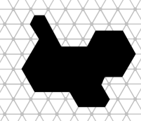
An object $\mathscr{O}$ is a subset $V_{\mathscr{O}}$ of points of $V_{\mathbb{T}}$ and let $G_{\mathscr{O}}=(V_{\mathscr{O}},E_{\mathscr{O}})$ be the subgraph of $G_{\mathbb{T}}$ induced by $V_{\mathscr{O}}$. The induced subgraph $G_{\mathscr{O}}$ is also called an object. We assume that $G_{\mathscr{O}}$ is connected, and Fig.6 illustrates the examples of two different objects.

(a)

(b)

Figure 6: Two examples of the objects

Now we define several subsets of the points on $\mathbb{T}$.

Definition 2

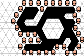
Surface Set $S(\mathscr{O})$. When object $\mathscr{O}$ is given, surface set $S(\mathscr{O})$ is a set of the points consists of every non-object point, i.e., point $v_{i}\notin V_{\mathscr{O}}$, which is adjacent to an object: $S(\mathscr{O})\cap V_{\mathscr{O}}=\emptyset$, and $\forall v_{i}\in S(\mathscr{O}),\exists v_{j}\in V_{\mathscr{O}}|(v_{i},v_{j})\in E_{\mathbb{T}}$.

Surface set $S(\mathscr{O})$ is determined when $\mathscr{O}$ is given and we simply denote $S(\mathscr{O})$ as $S$ if $\mathscr{O}$ is obvious. Now we define a different set of points which is a subset of $S(\mathscr{O})$.

Definition 3

Non-coating Set $N(\mathscr{O},\mathscr{R})$. When object $\mathscr{O}$ and set of robots $\mathscr{R}$ are given, non-coating set $N(\mathscr{O},\mathscr{R})$ is determined by every point $p_{i}$ in surface set $S(\mathscr{O})$ such that $p_{i}$ does not have two or more disjoint paths from the point occupied by any robot in $\mathscr{R}$ on $G_{\mathbb{T}}\setminus G_{\mathscr{O}}$.

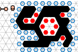
We simply denote $N(\mathscr{O},\mathscr{R})$ as $N$ if $\mathscr{O}$ and $\mathscr{R}$ are obvious. In Fig.7(a), all the circles (including the filled circles) describes the surface set $S$. And the filled circles illustrate the non-coating set $N(\subset S)$: some points are not reachable from any robot, and some points has no two or more disjoint paths from the robot due to an articulation point.

(a) Surface set and non-coating set

(b) Coating set occupied by the robots

Figure 7: Examples of surface set, non-coating set, and coating set

Definition 4

Coating Set $C(\mathscr{O},\mathscr{R})$. When object $\mathscr{O}$ and set of robots $\mathscr{R}$ are given, coating set $C(\mathscr{O},\mathscr{R})$ consists of every point in $S(\mathscr{O})$ which is not in $N(\mathscr{O},\mathscr{R})$: $C(\mathscr{O},\mathscr{R})=S(\mathscr{O})\setminus N(\mathscr{O},\mathscr{R})$.

We simply denote $C(\mathscr{O},\mathscr{R})$ as $C$ if $\mathscr{O}$ and $\mathscr{R}$ are obvious. Fig.7(b) illustrate a configuration that all the points in $C$ are occupied by the robots. Now we define the object coating problem using coating set when $\mathscr{O}$ and $\mathscr{R}$ are given.

Definition 5

Object Coating Problem. Given a set of $n$ robots ($n/2$ pairbots) $\mathscr{R}$ which are line-formed and they agree the direction to move. And given object $\mathscr{O}$, where $|C(\mathscr{O},\mathscr{R})|\leq n/2$, which are connected and located on the side of the direction to move agreed by the robots. Algorithm $\mathscr{A}$ solves the object coating problem if $\mathscr{R}$ satisfies all the following conditions when $\mathscr{A}$ terminates:

• All the points in coating set $C(\mathscr{O},\mathscr{R})$ are occupied by the robots in $\mathscr{R}$.

• All the pairbots are in short state.

• Algorithm $\mathscr{A}$ eventually terminates: algorithm $\mathscr{A}$ eventually reaches a configuration such that no robot can move.

(a) An initial configuration

(b) Coating with termination

Figure 8: An example of an object coating

Fig.8 illustrates an example of the object coating problem. Fig.8(a) presents an initial configuration. The robots in $\mathscr{R}$ are line-formed, and they agree label 1 ($\ell_{1}$) as the direction to move. Intuitively, the given line-formed set of robots executes marching algorithm introduced in the previous subsection during it does not recognize any object. If the head robot recognize any object, it changes the direction to move based on the agreed chirality, and the other robots follows the head robot, as a result, they surround the given object and terminate. In Fig.8(b), the object coating problem is solved because all the points in $C$ are occupied by the pairbots which are in short state. Note that some robots are remained, i.e., not on the points in $C$, when $n/2>|C(\mathscr{O},\mathscr{R})|$.

4.2 Object Coating Algorithm

In this subsection, we introduce an algorithm to solve the object coating problem. And we assume that the each robot can recognize whether itself is the head robot or not to terminate the proposed algorithm. To help to understand, we assume that the agreed direction to move is $\ell_{1}$ (positive direction of $X$ axis). Algorithm 2 represents an object coating algorithm when object $\mathscr{O}$ is given. In Algorithm 2, each robot locally executes function $\mathit{dir}()$ to determine the next direction to move, and move to the determined direction if some conditions are satisfied.

Algorithm 2 Object Coating Algorithm for robot $r_{i}$

assumption: The set of robots is line-formed on the line parallel to $X$ axis. Given object $\mathscr{O}$ such that $G_{\mathscr{O}}$ is connected and located on the side of the direction to move.

variables and functions:

$~{}\cdot~{}\ell_{x}$, $\mathit{buddy}$, $\mathit{occupy}(\ell_{x})$ :

The same as them in marching algorithm.

$~{}\cdot~{}O$ :

The set variable consisting of the local labels where an object exists: $O\subseteq\{\ell_{1},\ell_{2},\ldots,\ell_{6}\}$. If there is no object in adjacent points, $O=\emptyset$.

$~{}\cdot~{}\mathit{next}(\ell_{x},s)$ :

The function returns a local label $\ell_{y}$ where $y=(((x-1+s)\bmod 6)+1)$. For example, $\mathit{next}(\ell_{3},2)=\ell_{5}$ or $\mathit{next}(\ell_{5},3)=\ell_{2}$.

$~{}\cdot~{}\mathit{isHead}$ :

A boolean variable becomes true if robot $r_{i}$ is the head robot, false otherwise.

$~{}\cdot~{}\mathit{dir}()$ :

The function returns the next direction to move as a local label using the following rules:

• if $(O=\emptyset)$ then $\ell_{1}$

• if $(O\neq\emptyset)\wedge(\exists\ell_{i}\in O|\{\mathit{next}(\ell_{i},1),\mathit{next}(\ell_{i},2),\mathit{next}(\ell_{i},3)\}\cap O=\emptyset)$ then $\mathit{next}(\ell_{i},1)$

• if $(O\neq\emptyset)\wedge(\exists\ell_{i}\in O|\mathit{next}(\ell_{i},1)\notin O,\mathit{occupy}(\mathit{next}(\ell_{i},2))\geq 1,\mathit{next}(\ell_{i},3)\in O)$

  then $\mathit{next}(\ell_{i},1)$

algorithm:

1:$(\mathit{buddy}=\ell_{0})\wedge(\mathit{isHead}=true)\wedge(\mathit{occupy}(\mathit{dir}())=0)\Rightarrow$ Exclusive move to $\mathit{dir}()$

2:$(\mathit{buddy}=\ell_{0})\wedge(\mathit{isHead}=false)\wedge(\mathit{occupy}(\mathit{dir}())=1)\Rightarrow$ Exclusive move to $\mathit{dir}()$

3:$(\mathit{buddy}\neq\ell_{0})\wedge(\mathit{occupy}(\mathit{dir}())=1)\wedge(\mathit{occupy}(\ell_{0})\geq 2)\wedge(\mathit{buddy}=\mathit{dir}())\Rightarrow$ Move to $\mathit{dir}()$

4:$(\mathit{buddy}\neq\ell_{0})\wedge(\mathit{occupy}(\mathit{dir}())=1)\wedge(O=\emptyset)\wedge(\mathit{occupy}(\ell_{4})=0)\wedge(\mathit{buddy}=\mathit{dir}())$ $\Rightarrow$ Move to $\mathit{dir}()$

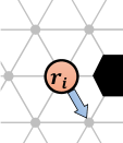
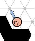
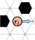
Fig.9 illustrates some examples that robot $r_{i}$ locally determines the direction to move (function $\mathit{dir}()$) when it recognizes an object, i.e., $r_{i}.O\neq\emptyset$ (rules 2 and 3 of function $\mathit{dir}()$). Note that robot $r_{i}$ does not recognize any object, it moves to the agreed direction (marching) by the first rule of function $\mathit{dir}()$. In Fig.9(a), $r_{i}$ determines $\ell_{2}$ to its direction to move because an object exists on $\ell_{1}$ and no object exists on $\ell_{2}$, $\ell_{3}$, and $\ell_{4}$ by the second rule of function $\mathit{dir}()$. For the same reason, in Fig.9(b), $r_{i}$ determines $\ell_{5}$ to its direction because no object exists on $\ell_{5}$, $\ell_{6}$, and $\ell_{1}$. Also in the case of Fig.9(c), $r_{i}$ determines $\ell_{1}$ to its direction because no object exists on $\ell_{1}$, $\ell_{2}$, and $\ell_{3}$, this prevents $r_{i}$ from move to non-coating points. The third rule of function $\mathit{dir}()$ can be satisfied only when two different objects located opposite to each other, e.g., $\ell_{2}$ and $\ell_{5}$. Fig.9(d) represents the case such that the third rule is satisfied. In this case, $r_{i}$ determines $\ell_{2}$ to its direction to move because $r_{j}$ exists on $\ell_{3}$, note that a robot may also exist on $r_{i}.\ell_{2}$.

(a)

(b)

(c)

(d)

Figure 9: Examples of the direction to move

Algorithm 2 is similar to marching algorithm (Algorithm 1): the pairbot in short state exclusively moves to the direction to move if one or less robot exists on the destination point, the pairbot in long state becomes short state by tail-sided robot (say $r_{i}$) move if another robot exists on the point occupied by $r_{i}$. However, different from marching algorithm, every robot repeatedly changes its direction to move based on the result of function $\mathit{dir}()$. Lines 1 and 2 are the executions for a pairbot in short state to make it long state, however the head robot never executes line 2 in order to avoid collision, i.e., two different pairbot which are in short state (exclusively) move to the same point, when the head robot return back after move around the object. Lines 3 and 4 are the executions for a pairbot in long state to make it short state. By line 3, the pairbot becomes short state when another robot exists on the point occupied tail-sided robot. Exceptionally, the tail robot in long state always becomes short state, if no other robot exists on the point occupied by head-sided robot. We omit the proof of an object coating algorithm because it can be easily proved by the similar manner of the proof of Algorithm 1.

5 Conclusion and Discussion

In this paper, we introduced a new computational model named Pairbot model consisting of paired robots called pairbots, which is based on LCM-model [1]. In the proposed model, each pairbot repeatedly changes its positional relation of the two robots, long and short, to achieve the goal. Moreover, as the basic problems of Pairbot model, we introduced two problems, the marching (linear movement) problem and the object coating problem, and proposed the two algorithms to solve these problems respectively to help to understand the computational power and limitations of Pairbot model.

Pairbot model has basically the similar variations of the assumptions, e.g., scheduler, geometric agreement, visibility, etc., however, it has one big different feature: every robot has one implicitly distinguishable robot as its buddy. In this paper, we introduced two simple problems only, however, we are considering various problems in Pairbot model, e.g., pattern formation (a line or a triangle), filling problem, or uniform deployment, as the future work then we have already solved some problems in Pairbot model. Interestingly, we found some problem which is not solvable in LCM-model but it is solvable in Pairbot model with the same capabilities (except the basic capabilities for Pairbot model), e.g., line formation from an arbitrary connected set of robots with 1-visibility range. We strongly expect that this special feature of Pairbot model provides many new possibilities in the field of autonomous mobile robots or the feasibility of a programmable matter.

Obviously, in LCM-model, if some additional capabilities are assumed, Pairbot model can be simulated by autonomous mobile robots in LCM-model. For example, if each robot has its unique identifier and is able to distinguish the other robot’s identifier, Pairbot model can be easily simulated. However, this assumption is too strong, this implies this capability (unique ID) provides the more computational power than Pairbot model. As the other way, luminous model (robots with light) is also considerable. If each robot has an internal light with 7 colors, it can be used for storing local label for its buddy. However, in this case, if an SSYNC or ASYNC scheduler is assumed, only one robot in a pairbot may be activated and this cannot guarantee the valid operation of pairbots. To clarify the minimum required capabilities for LCM-model to simulate Pairbot model as another future work.

References

- [1] Ichiro Suzuki and Masafumi Yamashita. Distributed anonymous mobile robots: Formation of geometric patterns. SIAM Journal on Computing, 28(4):1347–1363, 1999.
- [2] Paola Flocchini, Giuseppe Prencipe, and Nicola Santoro, editors. Distributed Computing by Mobile Entities, Current Research in Moving and Computing, volume 11340 of Lecture Notes in Computer Science. Springer, 2019.
- [3] Giuseppe Prencipe. Autonomous mobile robots: A distributed computing perspective. volume 8243, pages 6–21, 12 2014.
- [4] A. Hériban, X. Défago, and S. Tixeuil. Optimally gathering two robots. In Proc. of 19th Int. Conference on Distributed Computing and Networking (ICDCN), pages 1–10, 2018.
- [5] Taisuke Izumi, Samia Souissi, Yoshiaki Katayama, Nobuhiro Inuzuka, Xavier Défago, Koichi Wada, and Masafumi Yamashita. The gathering problem for two oblivious robots with unreliable compasses. SIAM Journal on Computing, 41, 11 2011.
- [6] Giuseppe Prencipe. Impossibility of gathering by a set of autonomous mobile robots. Theor. Comput. Sci., 384:222–231, 10 2007.
- [7] S. Cicerone, Di Stefano, and A. Navarra. Gathering of robots on meeting-points. Distributed Computing, 31(1):1–50, 2018.
- [8] M. Cieliebak, P. Flocchini, G. Prencipe, and N. Santoro. Distributed computing by mobile robots: Gathering. SIAM Journal on Computing, 41(4):829–879, 2012.
- [9] P. Flocchini, G. Prencipe, N. Santoro, and P. Widmayer. Gathering of asynchronous robots with limited visibility. Theoretical Computer Science, 337(1–3):147–169, 2005.
- [10] S. Kamei, A. Lamani, F. Ooshita, and S. Tixeuil. Asynchronous mobile robot gathering from symmetric configurations without global multiplicity detection. In 18th SIROCCO, pages 150–161, 2011.
- [11] Paola Flocchini, Giuseppe Prencipe, Nicola Santoro, Peter Widmayer, Alok Aggarwal, and C. Rangan. Hard tasks for weak robots: The role of common knowledge in pattern formation by autonomous mobile robots. volume 1741, pages 93–102, 01 1999.
- [12] Paola Flocchini, Giuseppe Prencipe, Nicola Santoro, and Peter Widmayer. Arbitrary pattern formation by asynchronous, anonymous, oblivious robots. Theoretical Computer Science, 407:412–447, 11 2008.
- [13] Ioannis Chatzigiannakis, Michael Markou, and Sotiris Nikoletseas. Distributed circle formation for anonymous oblivious robots. volume 3059, pages 159–174, 05 2004.
- [14] P. Flocchini, N. Santoro, G. Viglietta, and M. Yamashita. Rendezvous with constant memory. Theoretical Computer Science, 621:57–72, 2016.
- [15] T. Okumura, K. Wada, and X. Défago. Optimal rendezvous -algorithms for asynchronous mobile robots with external-lights. In Proc. of the 22nd Int. Conference on Principles of Distributed Systems (OPODIS), pages 24:1–24:16, 2018.
- [16] T. Okumura, K. Wada, and Y. Katayama. Brief announcement: Optimal asynchronous rendezvous for mobile robots with lights. In Proc. of the 19th Int. Symposium on Stabilization, Safety, and Security of Distributed Systems (SSS), pages 484–488, 2017.
- [17] Z. Bouzid, S. Das, and S. Tixeuil. Gathering of mobile robots tolerating multiple crash faults. In the 33rd Int. Conf. on Distributed Computing Systems, pages 334–346, 2013.
- [18] S. Souissi, X. Défago, and M. Yamashita. Using eventually consistent compasses to gather memory-less mobile robots with limited visibility. ACM Transactions on Autonomous and Adaptive Systems, 4(1):1–27, 2009.
- [19] P. Flocchini, G. Prencipe, N. Santoro, and P. Widmayer. Arbitrary pattern formation by asynchronous oblivious robots. Theoretical Computer Science, 407:412–447, 2008.
- [20] N. Fujinaga, Y. Yamauchi, H. Ono, S. Kijima, and M. Yamashita. Pattern formation by oblivious asynchronous mobile robots. SIAM Journal on Computing, 44(3):740–785, 2015.
- [21] Y. Yamauchi, T. Uehara, S. Kijima, and M. Yamashita. Plane formation by synchronous mobile robots in the three-dimensional euclidean space. Journal of the ACM, 64:3(16):16:1–16:43, 2017.
- [22] V. Gervasi and G. Prencipe. Coordination without communication: The case of the flocking problem. Discrete Applied Mathematics, 144(3):324–344, 2004.
- [23] Vincenzo Gervasi and Giuseppe Prencipe. Coordination without communication: the case of the flocking problem. Discrete Applied Mathematics, 144:324–344, 12 2004.
- [24] S. Souissi, T. Izumi, and K. Wada. Oracle-based flocking of mobile robots in crash-recovery model. In Proceedings of the 11th International Symposium on Stabilization, Safety, and Security of Distributed Systems (SSS), pages 683–697, 2009.
- [25] Shantanu Das, Paola Flocchini, Giuseppe Prencipe, and Masafumi Yamashita. Autonomous mobile robots with lights. Theoretical Computer Science, 609, 09 2015.
- [26] M. D’Emidio, D. Frigioni, and A. Navarro. Synchronous robots vs asynchronous lights-enhanced robots on graphs. Electr. Notes Theor. Comput. Sci., 322:169–180, 2016.
- [27] G. Luna, Paola Flocchini, Sruti Gan Chaudhuri, F. Poloni, and Giovanni Viglietta. Mutual visibility by luminous robots without collisions. Information and Computation, 03 2015.
- [28] Giovanni Viglietta. Rendezvous of two robots with visible bits. volume 8243, 11 2012.
- [29] Seth Copen Goldstein, Jason D. Campbell, and Todd C. Mowry. Programmable matter. IEEE Computer, 38(6):99–101, Jun 2005.
- [30] A. L. Yarin. Nanofibers, nanofluidics, nanoparticles and nanobots for drug and protein delivery systems. Scientia Pharmaceutica, 78(3):542–542, 2010.
- [31] Seth Copen Goldstein and Todd C. Mowry. Claytronics: A scalable basis for future robots. In RoboSphere 2004, Moffett Field, CA, November 2004.
- [32] Ram Ravichandran, Geoffrey Gordon, and Seth Goldstein. A scalable distributed algorithm for shape transformation in multi-robot systems. pages 4188–4193, 10 2007.
- [33] Zahra Derakhshandeh, Shlomi Dolev, Robert Gmyr, Andréa Richa, Christian Scheideler, and Thim Strothmann. Brief announcement: Amoebot-a new model for programmable matter. Annual ACM Symposium on Parallelism in Algorithms and Architectures, 06 2014.
- [34] Joshua Daymude, Zahra Derakhshandeh, Robert Gmyr, Alexandra Porter, Andréa Richa, Christian Scheideler, and Thim Strothmann. On the runtime of universal coating for programmable matter. Natural Computing, 17, 11 2017.
- [35] Joshua Daymude, Robert Gmyr, Andréa Richa, Christian Scheideler, and Thim Strothmann. Improved Leader Election for Self-organizing Programmable Matter, pages 127–140. 12 2017.
- [36] Joshua Daymude, Robert Gmyr, Kristian Hinnenthal, Irina Kostitsyna, Christian Scheideler, and Andréa Richa. Convex hull formation for programmable matter. pages 1–10, 01 2020.