Modulation of Landau levels and de Haas-van Alphen oscillation in magnetized graphene by uniaxial tensile strain/ stress

Abstract

The strain engineering technique allows us to alter the electronic properties of graphene in various ways. Within the continuum approximation, the influences of strain result in the appearence of a pseudo-gauge field and modulated Fermi velocity. In this study, we investigate theoretically the effect of linear uniaxial tensile strain and/or stress, which makes the Fermi velocity anisotropic, on a magnetized graphene sheet in the presence of an applied electrostatic voltage. More specifically, we analyze the consequences of the anisotropic nature of the Fermi velocity on the structure Landau levels and de Haas - van Alphen (dHvA) quantum oscillation in the magnetized graphene sheet. The effect of the direction of the applied strain has also been discussed.

1 Introduction

Fifteen years ago, the first fabrication of monolayer graphene opened a new era in condensed matter physics as well as materials science [1, 2]. This was not only the first synthesized atomically thin monolayer but also the first two dimensional Dirac material. Electrons related to $2p_{z}$ orbital in the honeycomb lattice of graphene surprisingly behave as massless relativistic fermions in $(2+1)$ dimensional space time [3]. Due to Klein tunneling, only magnetic fields can trap these particles to form the relativistic Landau levels [4, 5, 6, 7, 8, 9, 10, 11]. The confining electrons in graphene in magnetic fields open up new possibilities to study some very interesting phenomena such as quantum Hall effect [12, 13, 14], de Haas - van Alphen (dHvA) oscillation [15, 16, 17, 18] or collapse of Landau levels [19, 20, 21] etc. The last phenomenon, namely the collapse of Landau levels, takes place when an electrostatic voltage applied to the magnetized graphene sheet reaches a critical value. In contrast to the magnetic field, the in-plane electric field opposes the formation of Landau levels and consequently the Landau levels collapse if the electric field is large enough [19, 20, 21, 22]. Because of this effect, it is possible to modulate the dHvA oscillation in graphene’s magnetization by electric field [16, 17, 18].

It is now known that electronic properties of graphene change when it is subjected to mechanical deformation and manipulating the electronic properties in this way is known as the strain engineering technique. Deforming a graphene sheet can produce a pseudoelectromagnetic field [23, 24, 25, 26, 27, 28, 29]. Interestingly this pseudoelectromagnetic field depends on the valleys the electrons belong to. These fields not only act similarly to the real electromagnetic field, but the pseudoelectromagnetic fields also open a new avenue to control the valley current of the electron in graphene i.e valleytronics [23, 24, 25, 26, 27, 28, 29, 30]. Recently the strain engineering technique has also been used to control the dHvA oscillation besides using an external electric field [31]. Apart from the induced pseudoelectromagnetic field, another consequence of deformation or strain is the modulation of Fermi velocity. Unlike unstrained graphene with well-known constant Fermi velocity $v_{F}\approx c/300$, straining graphene sheet can make Fermi velocity becomes inhomogeneous or anisotropic [30, 32, 33, 34, 35, 36]. Interestingly electrons can be bound in the presence of inhomogeneous magnetic fields and anisotropic Fermi velocity [37, 38, 39]. In the latter case, the Fermi velocity in zigzag and armchair direction becomes different resulting in the Dirac cones being tilted [4], and consequently the electronic properties of the graphene sheet under applied external fields depend on the direction of fields and strain. For example, in Refs. [21, 37], the collapse of Landau levels under a crossed electromagnetic field with uniaxial strain has been studied. The critical electric field depends not only on the magnitude but also on the direction of the applied strain.

In view of the above observations, we feel it would be of interest to examine how uniaxial tensile strain or stress affects the Landau levels and also the dHvA oscillation in magnetized graphene. This could provide a mechanical way to modulate magnetic properties of monolayer graphene. To achieve this purpose, we shall consider a deformed graphene sheet under the influence of a perpendicular magnetic field combining with an in-plane electric field. Solving the Dirac-Weyl equation by using the concept of supersymmetric quantum mechanics [40], we shall determine the Landau levels analytically. Following some earlier works [15, 41], we calculate analytically the chemical potential and magnetization of graphene sheet at zero temperature. It is shown that the influence of zigzag strain on the quantum oscillation of both the chemical potential and the magnetization is more significant in comparison with the armchair strain when there is an applied electric field. The organization of the paper is as follows: in Section 2 we derive the solutions of the Dirac-Weyl equation i.e. the Landau levels for deformed graphene under crossed electromagnetic fields; in 3 we study collapse of Landau levels; in Section 4 we examine dHvA oscillation of magnetization; in Section 5, we discuss the case when direction of the applied electric field is changed; finally, Section 6 is devoted to a conclusion.

2 Dynamics of electrons in uniaxially deformed graphene sheet under crossed electromagnetic fields

Consider a graphene sheet with size $L_{x}\times L_{y}$ ($L_{x},L_{y}\gg a$, $a\approx 1.42\text{\AA}$ is lattice constant) being deformed by a uniaxial tensile strain or stress

$$u_{x}=\epsilon_{Z}x,\quad u_{y}=\epsilon_{A}y,$$ (1)

where $x$ and $y$ axes are parallel to zigzag (ZZ) and armchair (AC) directions respectively. The domains of the coordinates are $-L_{x}/2\leq x\leq L_{x}/2$ and $-L_{y}/2\leq y\leq L_{y}/2$ while $\epsilon_{Z,A}>0$ ($\epsilon_{Z,A}<0$) represents the strength of tensile strain (or stress). The strain tensor is a diagonal one given by [42]

$$u_{xx}=\partial_{x}u_{x}=\epsilon_{Z},\quad u_{yy}=\partial_{y}u_{y}=\epsilon_{A},\quad u_{xy}=\frac{1}{2}\left(\partial_{x}u_{y}+\partial_{y}u_{x}\right)=0.$$ (2)

As a result of this deformation, not only the pseudo-gauge potential

$$\left\{\begin{array}[]{l}A_{x}^{(s)}=\dfrac{\eta\beta\hbar}{2ea}\left(u_{xx}-u_{yy}\right)=\dfrac{\eta\beta\hbar}{2ea}\left(\epsilon_{Z}-\epsilon_{A}\right),\\ A_{y}^{(s)}=\dfrac{\eta\beta\hbar}{ea}u_{xy}=0,\\ \phi^{(s)}=g\left(u_{xx}+u_{yy}\right)=g\left(\epsilon_{Z}+\epsilon_{A}\right),\end{array}\right..$$ (3)

is induced but also the Fermi velocity becomes anisotropic

$$v_{xx}=v_{F}\left((1+(1-\beta)\epsilon_{Z}\right),\quad v_{yy}=v_{F}\left((1+(1-\beta)\epsilon_{A}\right),\quad v_{xy}=0.$$ (4)

Here the Fermi velocity is $v_{F}\approx 10^{6}\text{ m/s}$, $\beta\approx 2-3$ is Grüneisen parameter, $g\approx 4-20\text{ V}$ is acoustic coupling constant and $\eta=\pm 1$ is valley index ($K$ or $K^{\prime}$ valley) [24, 34]. However, since the induced pseudo-gauge field is space independent, it does not produce pseudo electromagnetic fields. Meanwhile, to confine the electron, it is necessary to apply a constant electromagnetic field such that the magnetic field is perpendicular to the graphene surface while the electric field is along armchair direction as follows:

$$\vec{B}=B\vec{e}_{z},\quad\vec{E}=E\vec{e}_{y},$$ (5)

Then corresponding gauge potentials are

$$A_{x}^{(a)}=-By,\quad A_{y}^{(a)}=0,\quad\phi^{(a)}=-Ey-g\left(\epsilon_{Z}+\epsilon_{A}\right).$$ (6)

Therefore, the low excited electrons are governed by the following stationary 2D Dirac-Weyl equation:

$$\left\{\eta v_{xx}\sigma_{x}\left(\hat{p}_{x}+eA_{x}^{(s)}+eA_{x}^{(a)}\right)+v_{yy}\sigma_{y}\hat{p}_{y}-e\left(\phi^{(s)}+\phi^{(a)}(y)\right)\right\}\Psi(x,y)=\mathcal{E}\Psi(x,y),$$ (7)

where the linear momentum operators are $\hat{p}_{x,y}=-i\hbar\partial_{x,y}$ and $\sigma_{x,y}$ are Pauli matrices. It can be seen from the above equation that the linear momentum along $x$-axis is conversed, hence, the pseudospinor can be separated as $\Psi(x,y)=\exp{\left(ik_{x}x\right)}\psi(y)$. Due to the Born-von Karman boundary condition, the wave number $k_{x}$ must be quantized as $k_{x}=2\pi N_{x}/L_{x}$.

Now, by introducing new notations: cyclotron length $l_{B}=\sqrt{\hbar/eB}$, dimensionless ratio $\alpha=E/(v_{F}B)$, strain-induced $k_{s}=\beta(\epsilon_{Z}-\epsilon_{A})/2a$ and energy wave-number $\varepsilon=\mathcal{E}/(\hbar v_{F})$, Eq. (7) can be rewritten as

$$\left[i\sigma_{y}\partial_{y}-\dfrac{\eta\left(1+(1-\beta)\epsilon_{Z}\right)}{1+(1-\beta)\epsilon_{A}}\left(k_{x}+\eta k_{s}-\dfrac{y}{l_{B}^{2}}\right)\sigma_{x}\right.$$

$$\left.-\dfrac{\alpha y}{\left(1+(1-\beta)\epsilon_{A}\right)l_{B}^{2}}+\dfrac{\varepsilon}{1+(1-\beta)\epsilon_{A}}\right]\psi(y)=0.$$ (8)

Rotating the pseudospinor $\psi(y)$ into $\tilde{\psi}(y)$ as [21, 22, 39, 43]

$$\psi(y)=\exp\left(\dfrac{\sigma_{x}}{4}\ln\left(\dfrac{\left(1+(1-\beta)\epsilon_{Z}\right)+\eta\alpha}{\left(1+(1-\beta)\epsilon_{Z}\right)-\eta\alpha}\right)\right)\tilde{\psi}(y),$$ (9)

Eq. (2) becomes

$$\begin{pmatrix}0&\partial_{y}+W(y)\\ -\partial_{y}+W(y)&0\end{pmatrix}\begin{pmatrix}\tilde{\psi}(y)_{+}\\ \tilde{\psi}(y)_{-}\end{pmatrix}={\tilde{\varepsilon}}\begin{pmatrix}\tilde{\psi}(y)_{+}\\ \tilde{\psi}(y)_{-}\end{pmatrix},$$ (10)

where

$$W(y)=\dfrac{\sqrt{\left(1+(1-\beta)\epsilon_{Z}\right)^{2}-\alpha^{2}}}{\left(1+(1-\beta)\epsilon_{A}\right)l_{B}^{2}}y-\dfrac{\eta\left[\alpha\varepsilon-\left(1+(1-\beta)\epsilon_{Z}\right)^{2}\left(k_{x}+\eta k_{s}\right)\right]}{\left(1+(1-\beta)\epsilon_{A}\right)\sqrt{\left(1+(1-\beta)\epsilon_{Z}\right)^{2}-\alpha^{2}}},$$ (11)

and

$${\tilde{\varepsilon}}=\dfrac{\left(1+(1-\beta)\epsilon_{Z}\right)\left[-\varepsilon+\alpha\left(k_{x}+\eta k_{s}\right)\right]}{\left(1+(1-\beta)\epsilon_{A}\right)\sqrt{\left(1+(1-\beta)\epsilon_{Z}\right)^{2}-\alpha^{2}}}.$$ (12)

Eq. (10) indicates the supersymmetric nature of the problem [40]. Following the supersymmetry formalism [40], we act on the left of Eq. (10) by the operator

$$\begin{pmatrix}0&\partial_{y}+W(y)\\ -\partial_{y}+W(y)&0\end{pmatrix}.$$

Then we obtain the following two independent second-order ordinary differential equations:

$$\left[-\partial_{y}^{2}+W^{2}(y)\pm\dfrac{dW}{dy}\right]{\tilde{\psi}}_{\pm}(y)=(\tilde{\varepsilon})^{2}{\tilde{\psi}}_{\pm}(y).$$ (13)

These can be regarded as a pair of energy dependent Schrödinger equations [44] corresponding to 1D shifted harmonic oscillators [40]

$$W^{2}(y)\pm\dfrac{dW}{dy} =\dfrac{\left(1+(1-\beta)\epsilon_{Z}\right)^{2}-\alpha^{2}}{\left(1+(1-\beta)^{2}\epsilon_{A}\right)l_{B}^{4}}\left\{y-\dfrac{\eta l_{B}^{2}\left[\alpha\varepsilon-\left(1+(1-\beta)\epsilon_{Z}\right)^{2}\left(k_{x}+\eta k_{s}\right)\right]}{\left(1+(1-\beta)\epsilon_{Z}\right)^{2}-\alpha^{2}}\right\}^{2}$$ (14)

$$\pm\dfrac{\sqrt{\left(1+(1-\beta)\epsilon_{Z}\right)^{2}-\alpha^{2}}}{\left(1+(1-\beta)\epsilon_{A}\right)l_{B}^{2}}.$$

Hence, from the discrete spectrum of shifted harmonic oscillator, we easily determine the eigenvalue $\varepsilon_{n,\eta}(k_{x})$ i.e the Landau levels

$$\mathcal{E}_{n,\eta}(k_{x})=\dfrac{\hbar E}{B}k_{x}^{*}+\text{sign}(n)\sqrt{2|n|eB^{*}\hbar v_{F}^{2}},\quad n=0,\pm 1,\pm 2,\ldots.$$ (15)

Here the effective $x$-component of momentum $k_{x}^{*}$ and the effective magnetic field strength $B^{*}$ are both strain-dependent:

$$k_{x}^{*}=k_{x}+\dfrac{\eta\beta}{2a}\left(\epsilon_{Z}-\epsilon_{A}\right),$$ (16)

$$B^{*}=\dfrac{\left(\left(1+(1-\beta)\epsilon_{Z}\right)^{2}v_{F}^{2}B^{2}-E^{2}\right)^{3/2}\left(1+(1-\beta)\epsilon_{A}\right)}{\left(1+(1-\beta)\epsilon_{Z}\right)^{2}v_{F}^{3}B^{2}}.$$ (17)

Noticeably, the spectrum in Eq. (15) remains unchanged under the valley-momentum transformation:

$$\mathcal{E}_{n,-\eta}\left(k_{x}+\dfrac{2\eta\beta}{a}(\epsilon_{Z}-\epsilon_{A})\right)=\mathcal{E}_{n,+\eta}\left(k_{x}\right).$$

It may be noted that beside the spin degeneracy $g_{spin}=2$, the Landau levels are also valley degenerated $g_{valley}=2$ and the influence of strain-induced vector potential is nothing more than translating $x$-axis momentum, in other words, it is similar to the Aharonov-Bohm effect. Also when there is no deformation $\epsilon_{Z}=\epsilon_{A}=0$, the spectrum $\mathcal{E}_{n,\eta}(k_{x})$ coincides to known results in Refs. [16, 17, 18].

Since the potential (14) is of harmonic oscillator shifted by

$$y_{n,\eta}(k_{x})=\dfrac{\eta\hbar}{eB}\left(\dfrac{\text{sign}(n)EB\sqrt{2|n|eB^{*}v_{F}^{2}/\hbar}}{\left(1+(1-\beta)\epsilon_{Z}\right)^{2}v_{F}^{2}B^{2}-E^{2}}-k_{x}^{*}\right),$$ (18)

the Landau levels are centered around $y_{n,\eta}(k_{x})$ and consequently, only the ones which satisfy the following condition

$$-\dfrac{L_{y}}{2}\leq y_{n,\eta}(k_{x})\leq\dfrac{L_{y}}{2},$$

are localized inside graphene sheet. Explicitly this condition reads

$$k_{-}\leq k_{x}\leq k_{+},\quad k_{\pm}=\dfrac{\text{sign}(n)EB\sqrt{2|n|eB^{*}v_{F}^{2}/\hbar}}{\left(1+(1-\beta)\epsilon_{Z}\right)^{2}v_{F}^{2}B^{2}-E^{2}}-\dfrac{\eta\beta}{2a}\left(\epsilon_{Z}-\epsilon_{A}\right)\pm\dfrac{eBL_{y}}{2\hbar}.$$ (19)

From now on we shall consider just one valley, say $\eta=1$ ($K$ valley), since the results for the other valley would be identical.

3 Strain effect on Landau levels

For quantitative estimates, we apply a magnetic field of strength $B=20\text{ T}$ to the graphene sheet of dimension $1200a\times 600a$ and the Grüneisen parameter is $\beta=2$. Fig 1 illustrates Landau levels under different deformations when the electric field is $0.3\times 10^{6}\text{ V/m}$. As can be seen from Fig. 1, zigzag strain affects the Landau levels more in comparison with the armchair strain of the same magnitude. Not only the Landau levels are titled by the electric field, they are also centered at

$$\mathcal{E}_{n}=\text{sign}(n)\sqrt{2|n|eB^{**}\hbar v_{F}^{2}},\quad\text{where }B^{**}=\dfrac{\left(1+(1-\beta)\epsilon_{A}\right)\left(1+(1-\beta)\epsilon_{Z}\right)^{2}v_{F}B^{2}}{\sqrt{\left(1+(1-\beta)\epsilon_{Z}\right)^{2}v_{F}^{2}B^{2}-E^{2}}},$$ (20)

instead of $\text{sign}(n)\sqrt{2|n|eB^{*}\hbar v_{F}^{2}}$. These are the Landau levels corresponding to the momentum $k^{**}=(k_{+}+k_{-})/2$. Comparing to (15) and (18), the Landau levels can be written as a sum of two parts:

$$\mathcal{E}_{n,\eta}=\mathcal{E}_{n}+\eta eEy_{n,\eta},$$

where the second part can be interpreted as electric potential at center of the pseudospinor.

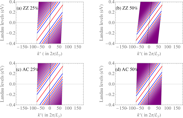
Figure 1: Landau levels of ${1200a\times 600a}$ graphene sheet under different deformations when the electric field is $0.3\times 10^{6}\text{ V/m}$ and magnetic field is $20\text{ T}$ i.e the corresponding $\alpha=E/(v_{F}B)=0.015$. The black lines show the centers of Landau levels. ZZ and AC are presented for zigzag and armchair deformation respectively while the magnitude of the deformation $\epsilon_{Z,A}$ is expressed by percentage.

Similar to the collapse of Landau levels in unstrained graphene, in the case of strained graphene the Landau levels collapse at a critical electric field depending on strain and is given by

$$E_{c}=\left(1+(1-\beta)\epsilon_{Z}\right)v_{F}B.$$ (21)

This formula suggests zigzag strain affects both spacing between the Landau levels and value of the critical electric field strength while armchair strain modulates the spacing only. Fig 2 below illustrates the spacing between first three excited Landau levels (from $n=1$ to $n=3$) and lowest Landau level $n=0$ near $K/K^{\prime}$ valley depends on electric field strength.

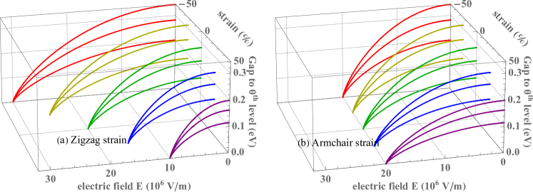
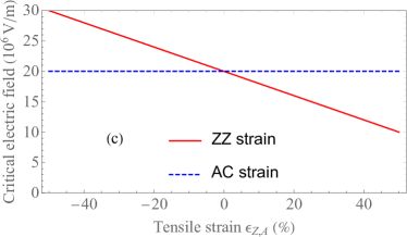
Figure 2: Modulation of Landau levels by tensile strain $\epsilon_{Z,A}$ near $K/K^{\prime}$ valley. (a) Since $\beta\approx 2$, larger zigzag strain pulls the critical electric field to the left while larger zigzag stress pushes the critical electric field to the right. (b) Armchair strain or stress does not affect on the critical electric field. (c) The critical electric field $E_{c}$ as function of zigzag (red) and armchair (blue dashed) tensile strain $\epsilon_{Z,A}$.

4 Modulation of the magnetization by uniaxial strain

At zero temperature, all of negative energy levels are fully filled by Dirac sea and graphene exhibits the property of semimetal material. However, when doping electrons into graphene with a concentration $N_{0}$, the Fermi level i.e chemical potential moves upward to $\mu_{0}=\sqrt{\pi N_{0}\hbar^{2}v_{F}^{2}}$ and all energy levels between $0$ and $\mu_{0}$ are filled. Thus graphene now exhibits features of metalic material in which de Haas-van Alphen (dHvA) effect may occur. To investigate the influence of deformation on dHvA effect, we need to determine the magnetization per area $M$ of graphene sheet via the free energy per area $F$:

$$M=-\dfrac{dF}{dB},\quad F=\dfrac{1}{L_{x}L_{y}}\sum_{\text{filled }n,k_{x}}\varepsilon_{n,k_{x}}.$$ (22)

Taking into account the quantization of the momentum $k_{x}$ by $\delta k_{x}=2\pi/L_{x}$ as well as the valley and spin degeneracy, the number of localized Landau states per unit area corresponding to each quantum number $n$ is $D(B)=g_{valley}g_{spin}(k_{+}-k_{-})/\delta k_{x}=2eB/\pi\hbar$. Following Refs. [16, 17], we can determine the chemical potential at zero temperature as the magnetic energy $\sqrt{2neB^{**}\hbar v_{F}^{2}}$ at $n=\left\lfloor N_{0}/D(B)\right\rfloor+1$:

$$\dfrac{\mu(B,E)}{\mu_{0}}=\sqrt{\dfrac{\left(1+(1-\beta)\epsilon_{A}\right)\left(1+(1-\beta)\epsilon_{Z}\right)^{2}v_{F}B}{\sqrt{\left(1+(1-\beta)\epsilon_{Z}\right)^{2}v_{F}^{2}B^{2}-E^{2}}}\dfrac{\left\lfloor\nu\right\rfloor+1}{\nu}}.$$ (23)

Next we introduce the filling factor $\nu=\mu_{0}^{2}/2eB\hbar v_{F}^{2}$ and the floor function $\left\lfloor\nu\right\rfloor$. Subsequently the free energy per unit area $F$ can be found to be

$$F(B,E)= \sqrt{\dfrac{8e^{3}B^{2}B^{**}v_{F}^{2}}{\pi^{2}\hbar}}\left[\xi\left(-\dfrac{1}{2}\right)-\xi\left(-\dfrac{1}{2},\left\lfloor\nu\right\rfloor+1\right)+\left(\left\{\nu\right\}-\dfrac{1}{2}\right)\sqrt{\left\lfloor\nu+1\right\rfloor}\right]+$$ (24)

$$+\left\{\nu\right\}\left(\left\{\nu\right\}-1\right)\dfrac{e^{2}EBL_{y}}{2\pi\hbar},$$

where the fractional part of $\nu$ is $\left\{\nu\right\}=\nu-\left\lfloor\nu\right\rfloor$, $\xi(-1/2)\approx-0.207886$ and $\xi(-1/2,x)$ is Hurwitz zeta function [45]. The last term of the free energy comes from the difference of energy due to the electric field when the $(\left\lfloor\nu\right\rfloor+1)-$th Landau level is partially filled. As can be seen from the expression of the chemical potential and free energy, the ceiling or floor functions are piecewise function and only continuously vary when the filling factor is between two integers $n\leq\nu<n+1$. Thus the discontinuous profile of the free energy can be seen with the period $\Delta(1/B)=2e\hbar v_{F}^{2}/\mu_{0}^{2}$ corresponds to $\Delta\nu=1$. From Eqs. (22) and (24), the magnetization per unit area at zero temperature can be determined as

$$M(B,E)= -\dfrac{3\left(1+(1-\beta)\epsilon_{Z}\right)^{2}v_{F}^{2}B^{2}-4E^{2}}{2\left[\left(1+(1-\beta)\epsilon_{Z}\right)^{2}v_{F}^{2}B^{2}-E^{2}\right]}\times$$ (25)

$$\times\sqrt{\dfrac{8e^{3}B^{**}v_{F}^{2}}{\pi^{2}\hbar}}\left[\xi\left(-\dfrac{1}{2}\right)-\xi\left(-\dfrac{1}{2},\left\lfloor\nu\right\rfloor+1\right)+\left(\left\{\nu\right\}-\dfrac{1}{2}\right)\sqrt{\left\lfloor\nu\right\rfloor+1}\right]+$$

$$-\left(1-\delta\left(\left\{\nu\right\}\right)\right)\sqrt{\dfrac{8e^{3}B^{**}v_{F}^{2}\nu^{2}\left(\left\lfloor\nu\right\rfloor+1\right)}{\pi^{2}\hbar}}-\left\{\nu\right\}\left(\left\{\nu\right\}-1\right)\dfrac{e^{2}EL_{y}}{2\pi\hbar}+$$

$$+\left(1-\delta\left(\left\{\nu\right\}\right)\right)\nu\left(\left\{\nu\right\}-\dfrac{1}{2}\right)\dfrac{e^{2}EL_{y}}{\pi\hbar}.$$

The Dirac $\delta$ function arises from the derivative of the fractional part $\left\{\nu\right\}$ which is undetermined i.e. it does not exist at integer value of filling factor $\nu$.

Let us now consider a graphene sheet as in Section 3 when it is negatively doped by electrons with a concentration $N_{0}\approx 290\;\mu\text{m}^{2}$ i.e. initial chemical potential is $\mu_{0}\approx 20\text{ meV}$. Fig 3 below show how chemical potential and magnetization curves are modulated by zigzag and armchair deformations.

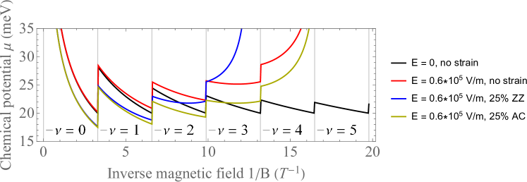
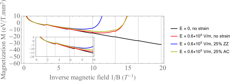
Figure 3: Chemical potential $\mu$ (above) and magnetization $M$ per unit area (below) versus inverse magnetic field strength $1/B$ under different configurations of applied electric field and strain: (black) no electric field and no strain, (red) $E=0.6\times 10^{5}\text{ V/m}$ with no strain, (blue) $E=0.6\times 10^{5}\text{ V/m}$ with $25\%$ zigzag strain and (yellow) $E=0.6\times 10^{5}\text{ V/m}$ with $25\%$ armchair strain. Grid lines correspond to integer filling factor $\nu=0$ to $\nu=5$.

From Section 3 it follows that if there is applied electrostatic voltage, Landau levels only exists when $E\leq\left(1+(1-\beta)\epsilon_{Z}\right)v_{F}B$. Also the chemical potential as well as magnetization per unit area oscillates with the period of $\Delta(1/B)=2e\hbar v_{F}^{2}/\mu_{0}^{2}$ which surprisingly solely depends on the magnetic field strength $B$ and does not depend on neither type of strain. Hence number of dHvA oscillation period is only $\nu_{max}=\left(1+(1-\beta)\epsilon_{Z}\right)\mu_{0}/2e\hbar v_{F}E$. Increasing the electric field will reduce this number of dHvA oscillation period. Noticeably the number of dHvA oscillation period is only controlled by zigzag strain. Fig. 3 shows this effect. The armchair strain only influences the magnitude of both the chemical potential and magnetization. This is a direct consequence from the fact that armchair strain only change the spacing between Landau levels but cannot induce a collapse as zigzag strain. The amplitude of oscillation is however quite small making it difficult to observe dHvA effect, thus it would be useful to separate the total magnetization (25) into three parts: regular term $M_{reg}$, oscillating term $M_{osc}$ and electric term $M_{elec}$. Since the oscillation arises from appearance of floor function of filling factor $\left\lfloor\nu\right\rfloor$, the regular magnetization and oscillating magnetization read

$$M_{reg}(B,E)=-\dfrac{3\left(1+(1-\beta)\epsilon_{Z}\right)^{2}v_{F}^{2}B^{2}-4E^{2}}{2\left[\left(1+(1-\beta)\epsilon_{Z}\right)^{2}v_{F}^{2}B^{2}-E^{2}\right]}\sqrt{\dfrac{8e^{3}B^{**}v_{F}^{2}}{\pi^{2}\hbar}}\left[\xi\left(-\dfrac{1}{2}\right)+\dfrac{2\nu^{3/2}}{3}\right],$$ (26)

and

$$M_{osc}(B,E)= -\dfrac{3\left(1+(1-\beta)\epsilon_{Z}\right)^{2}v_{F}^{2}B^{2}-4E^{2}}{2\left[\left(1+(1-\beta)\epsilon_{Z}\right)^{2}v_{F}^{2}B^{2}-E^{2}\right]}\times$$ (27)

$$\times\sqrt{\dfrac{8e^{3}B^{**}v_{F}^{2}}{\pi^{2}\hbar}}\left[-\dfrac{2\nu^{3/2}}{3}-\xi\left(-\dfrac{1}{2},\left\lfloor\nu\right\rfloor+1\right)+\left(\left\{\nu\right\}-\dfrac{1}{2}\right)\sqrt{\left\lfloor\nu\right\rfloor+1}\right]+$$

$$-\left(1-\delta\left(\left\{\nu\right\}\right)\right)\sqrt{\dfrac{8e^{3}B^{**}v_{F}^{2}\nu^{2}\left(\left\lfloor\nu\right\rfloor+1\right)}{\pi^{2}\hbar}}.$$

The third term of magnetization due to the electric field arises when the $(\left\lfloor\nu\right\rfloor+1)$th Landau level is partially filled and it vanishes when there is no electric field:

$$M_{elec}(B,E)=-\left\{\nu\right\}\left(\left\{\nu\right\}-1\right)\dfrac{e^{2}EL_{y}}{2\pi\hbar}+\left(1-\delta\left(\left\{\nu\right\}\right)\right)\nu\left(\left\{\nu\right\}-\dfrac{1}{2}\right)\dfrac{e^{2}EL_{y}}{\pi\hbar}.$$ (28)

Fig 4 below shows how electric field and strain can influence each term of magnetization. Electric field creates not only the $M_{elec}$ term and also reduces the oscillation in $M_{osc}$. Both zigzag and armchair strains do not affect $M_{elec}$. However, only zigzag strain significantly modulates the oscillating term of magnetization while the armchair strain do not. Since the magnitude of the oscillating term is dominated by the regular term, it is difficult to observe the dHvA effect in the total magnetization (see in Fig. 3). Note that, again, the period of quantum oscillations cannot be controlled by either the zigzag or the armchair strains because it only comes from the degeneracy of the Landau levels.

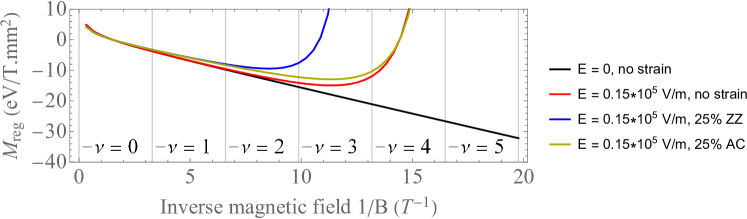
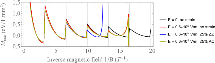
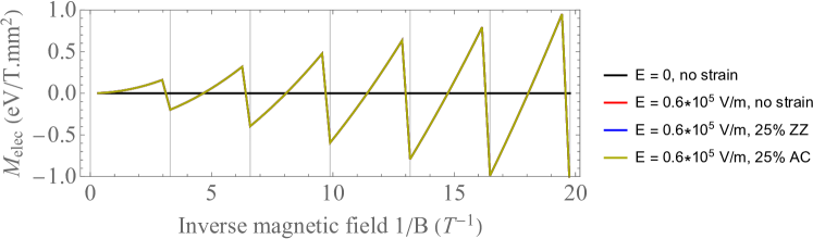
Figure 4: Each term of magnetization ($M_{reg},M_{osc},M_{elec}$) versus inverse magnetic field strength $1/B$ under different configurations of applied electric field and strain: (black) no electric field and no strain, (red) $E=0.6\times 10^{5}\text{ V/m}$ with no strain, (blue) $E=0.6\times 10^{5}\text{ V/m}$ with $25\%$ zigzag strain and (yellow) $E=0.6\times 10^{5}\text{ V/m}$ with $25\%$ armchair strain. Grid lines correspond to integer filling factor $\nu=0$ to $\nu=5$.

Also, since the regular component of our system mostly decreases (so long as the electric field is lower than the critical one) versus $1/B$, we may consider to measure the differential magnetic susceptibility $\chi=\frac{\partial M}{\partial H}\approx\mu_{0}\frac{\partial M}{\partial B}$ in the context of experiements. Then the regular term could be $\chi_{reg}=\mu_{0}\frac{\partial M}{\partial B}=-\frac{\mu_{0}}{B^{2}}\frac{\partial M}{\partial(1/B)}$ in which the last factor $\frac{\partial M}{\partial(1/B)}$ slightly varies i.e $B^{2}\chi_{reg}$ is almost a constant. Hence only the oscillation part $B^{2}\chi_{osc}$ and the electric part $B^{2}\chi_{elec}$ mainly contribute to the non constant profile of $B^{2}\chi$.

5 Discussion on changing direction of electric field

Finally, we would like to note that if the electric field is along the zigzag direction, the gauge potential should be of the form $A_{x}^{(a)}=0,A_{y}^{(a)}=Bx$ and $\phi^{(a)}=Ex$. Then the resulting Hamiltonian, at the first sight, is not as the same as in Eq. (7):

$$\hat{H}=\left\{\eta v_{xx}\sigma_{x}(\hat{p}_{x}+eA^{(s)}_{x})+v_{yy}\sigma_{y}(k+Bx)-eEx\right\}.$$ (29)

The cause of this apparently different form is due to the combination of strain-induced gauge potential $A_{x}^{(s)}$ and the momentum $\hat{p}_{x}$ to from a covariant derivative

$$\hat{p}_{x}+eA^{(s)}_{x}=-i\hbar\left(\partial_{x}+i\dfrac{eA^{(s)}_{x}}{\hbar}\right).$$

Fortunately, we can remove the strain-induced gauge potential $A_{x}^{(s)}$ by using a gauge transformation [46]. Explicitly, the pseudospinor $\Psi(x,y)$ should be transformed as

$$\Psi(x,y)=\exp{\left(-\dfrac{ieU(x)}{\hbar}\right)}\Psi^{\prime}(x,y).$$ (30)

When the covariant derivative $\hat{p}_{x}+eA^{(s)}_{x}$ is applied on Eq. (30), we obtain

$$\left(\hat{p}_{x}+eA^{(s)}_{x}\right)\Psi(x,y)=\exp{\left(-\dfrac{ieU(x)}{\hbar}\right)}\left(\hat{p}_{x}+eA^{(s)}_{x}-e\dfrac{dU(x)}{dx}\right)\Psi^{\prime}(x,y).$$ (31)

Thus $A_{x}^{(s)}$ can be eliminated when

$$\dfrac{dU(x)}{dx}=A^{(s)}_{x}\Rightarrow U(x)=\int A^{(s)}_{x}dx=A^{(s)}_{x}x.$$ (32)

Now, applying the gauge transformation found above, namely, $\Psi(x,y)=\exp{\left(-\dfrac{\imath eA^{(s)}_{x}x}{\hbar}\right)}\Psi^{\prime}(x,y)$, the Dirac-Weyl equation turns to

$$\hat{H}^{\prime}\Psi^{\prime}(x,y)=\mathcal{E}\Psi^{\prime}(x,y),$$ (33)

where the transformed Hamiltonian $\hat{H}^{\prime}$ is given as

$$\hat{H}^{\prime} =\exp\left(\imath\frac{eA^{s}_{x}x}{\hbar}\right)\hat{H}\exp\left(-\imath\frac{eA^{s}_{x}x}{\hbar}\right)$$ (34)

$$=\eta v_{xx}\sigma_{x}\hat{p}_{x}+v_{yy}\sigma_{y}(k+Bx)-eEx.$$

Thus the gauge transformed Hamiltonian $\hat{H}^{\prime}$ is identical to the one in Eq. (7) if $x$ is changed to $y$ and vice versa. Meanwhile the zigzag strain and the armchair strain would interchange their roles in dHvA oscillation of magnetization.

6 Conclusion

In summary, we have examined the effect of linear strain or stress on both the collapse of Landau levels and de Haas-van Alphen oscillation of magnetization in a magnetized graphene sheet in the presence of an electric field. The linear uniaxial strain makes Fermi velocity anisotropic, thus observation of physical quantities depends on the type of deformation or strain. As it has been shown here, the influence of zigzag strain is more significant than armchair strain because the former governs both the magnitude and the critical electric field strength for the Landau levels to exist while the latter only affects the spacing between the Landau levels. Consequently, only zigzag strain can control the number of oscillations in the magnetization of the graphene sheet. However, both kinds of strain cannot change the period of quantum oscillation in magnetization since it comes from the degeneracy of the Landau levels, which does not depend on strain.

References

-
[1]
K. S. Novoselov, A. K. Geim, S. V. Morozov, D. Jiang, M. I. Katsnelson, I. V.
Grigorieva, S. V. Dubonos, A. A. Firsov,
Two-dimensional gas of
massless dirac fermions in graphene, Nature 438 (7065) (2005) 197.
doi:10.1038/nature04233.
URL https://www.nature.com/articles/nature04233 -
[2]
Y. Zhang, Y.-W. Tan, H. L. Stormer, P. Kim,
Experimental observation
of the quantum hall effect and berry’s phase in graphene, Nature 438 (7065)
(2005) 201.
doi:10.1038/nature04235.
URL https://www.nature.com/articles/nature04235 -
[3]
A. H. Castro Neto, F. Guinea, N. M. R. Peres, K. S. Novoselov, A. K. Geim,
The electronic
properties of graphene, Reviews of Modern Physics 81 (2009) 109.
doi:10.1103/RevModPhys.81.109.
URL https://link.aps.org/doi/10.1103/RevModPhys.81.109 -
[4]
M. O. Goerbig,
Electronic
properties of graphene in a strong magnetic field, Rev. Mod. Phys. 83 (2011)
1193–1243.
doi:10.1103/RevModPhys.83.1193.
URL https://link.aps.org/doi/10.1103/RevModPhys.83.1193 -
[5]
Ş Kuru, J. Negro, L. M. Nieto,
Exact analytic
solutions for a dirac electron moving in graphene under magnetic fields,
Journal of Physics: Condensed Matter 21 (45) (2009) 455305.
doi:10.1088/0953-8984/21/45/455305.
URL http://stacks.iop.org/0953-8984/21/i=45/a=455305 -
[6]
M. R. Masir, P. Vasilopoulos, F. M. Peeters,
Graphene in
inhomogeneous magnetic fields: bound, quasi-bound and scattering states,
Journal of Physics: Condensed Matter 23 (31) (2011) 315301.
doi:10.1088/0953-8984/23/31/315301.
URL http://stacks.iop.org/0953-8984/23/i=31/a=315301 -
[7]
P. Roy, T. K. Ghosh, K. Bhattacharya,
Localization of
dirac-like excitations in graphene in the presence of smooth inhomogeneous
magnetic fields, Journal of Physics: Condensed Matter 24 (5) (2012) 055301.
doi:10.1088/0953-8984/24/5/055301.
URL http://stacks.iop.org/0953-8984/24/i=5/a=055301 -
[8]
C. A. Downing, M. E. Portnoi,
Massless dirac
fermions in two dimensions: Confinement in nonuniform magnetic fields,
Physical Review B 94 (2016) 165407.
doi:10.1103/PhysRevB.94.165407.
URL https://link.aps.org/doi/10.1103/PhysRevB.94.165407 -
[9]
D.-N. Le, V.-H. Le, P. Roy,
Conditional
electron confinement in graphene via smooth magnetic fields, Physica E:
Low-dimensional Systems and Nanostructures 96 (Supplement C) (2018) 17 – 22.
doi:https://doi.org/10.1016/j.physe.2017.09.025.
URL http://www.sciencedirect.com/science/article/pii/S1386947717313292 -
[10]
D.-N. Le, V.-H. Le, P. Roy,
Generalized
harmonic confinement of massless dirac fermions in (2+1) dimensions, Physica
E: Low-dimensional Systems and Nanostructures 102 (2018) 66 – 72.
doi:https://doi.org/10.1016/j.physe.2018.04.029.
URL http://www.sciencedirect.com/science/article/pii/S1386947718304351 -
[11]
D.-N. Le, P.-S. Luu, T.-S. Ha, N.-H. Phan, V.-H. Le,
Bound
states of (2+1)−dimensional massive dirac fermions in a lorentzian-shaped
inhomogeneous perpendicular magnetic field, Physica E: Low-dimensional
Systems and Nanostructures 116 (2020) 113777.
doi:https://doi.org/10.1016/j.physe.2019.113777.
URL http://www.sciencedirect.com/science/article/pii/S1386947719313669 -
[12]
K. I. Bolotin, F. Ghahari, M. D. Shulman, H. L. Stormer, P. Kim,
Observation of the
fractional quantum hall effect in graphene, Nature 462 (7270) (2009) 196.
doi:10.1038/nature08582.
URL https://www.nature.com/articles/nature08582 -
[13]
X. Du, I. Skachko, F. Duerr, A. Luican, E. Y. Andrei,
Fractional quantum hall
effect and insulating phase of dirac electrons in graphene, Nature
462 (7270) (2009) 192.
doi:10.1038/nature08522.
URL https://www.nature.com/articles/nature08522 -
[14]
D. T. Son, Is the
Composite Fermion a Dirac Particle?, Physical Review X 5 (3) (2015) 031027.
doi:10.1103/PhysRevX.5.031027.
URL https://link.aps.org/doi/10.1103/PhysRevX.5.031027 -
[15]
S. G. Sharapov, V. P. Gusynin, H. Beck,
Magnetic
oscillations in planar systems with the dirac-like spectrum of quasiparticle
excitations, Phys. Rev. B 69 (2004) 075104.
doi:10.1103/PhysRevB.69.075104.
URL https://link.aps.org/doi/10.1103/PhysRevB.69.075104 -
[16]
S. Zhang, N. Ma, E. Zhang,
The
modulation of the de Haas–van Alphen effect in graphene by electric
field, Journal of Physics: Condensed Matter 22 (11) (2010) 115302.
doi:10.1088/0953-8984/22/11/115302.
URL https://iopscience.iop.org/article/10.1088/0953-8984/22/11/115302 -
[17]
N. Ma, S. Zhang, D. Liu, E. Zhang,
Novel
electric field effects on magnetic oscillations in graphene nanoribbons,
Physics Letters A 375 (41) (2011) 3624–3633.
doi:10.1016/j.physleta.2011.08.034.
URL https://linkinghub.elsevier.com/retrieve/pii/S0375960111010073 -
[18]
Z. Alisultanov,
Landau
levels in graphene in crossed magnetic and electric fields: Quasi-classical
approach, Physica B: Condensed Matter 438 (2014) 41 – 44.
doi:https://doi.org/10.1016/j.physb.2013.12.033.
URL http://www.sciencedirect.com/science/article/pii/S0921452613008259 -
[19]
V. Lukose, R. Shankar, G. Baskaran,
Novel Electric
Field Effects on Landau Levels in Graphene, Physical Review Letters 98 (11)
(2007) 116802.
doi:10.1103/PhysRevLett.98.116802.
URL https://link.aps.org/doi/10.1103/PhysRevLett.98.116802 -
[20]
N. M. R. Peres, E. V. Castro,
Algebraic
solution of a graphene layer in transverse electric and perpendicular
magnetic fields, Journal of Physics: Condensed Matter 19 (40) (2007)
406231.
doi:10.1088/0953-8984/19/40/406231.
URL http://iopscience.iop.org/article/10.1088/0953-8984/19/40/406231 -
[21]
P. Ghosh, P. Roy, Collapse
of landau levels in graphene under uniaxial strain, Materials Research
Express 6 (12) (2019) 125603.
doi:10.1088/2053-1591/ab52ad.
URL https://doi.org/10.1088/2F2053-1591/2Fab52ad -
[22]
D. Nath, M. Presilla, O. Panella, P. Roy,
Non-commutativity
effects in the Dirac equation in crossed electric and magnetic fields, EPL
(Europhysics Letters) 123 (2) (2018) 20008.
doi:10.1209/0295-5075/123/20008.
URL http://stacks.iop.org/0295-5075/123/i=2/a=20008 -
[23]
M. A. H. Vozmediano, F. de Juan, A. Cortijo,
Gauge fields and
curvature in graphene, Journal of Physics: Conference Series 129 (2008)
012001.
doi:10.1088/1742-6596/129/1/012001.
URL http://stacks.iop.org/1742-6596/129/i=1/a=012001 -
[24]
M. Vozmediano, M. Katsnelson, F. Guinea,
Gauge
fields in graphene, Physics Reports 496 (4) (2010) 109 – 148.
doi:https://doi.org/10.1016/j.physrep.2010.07.003.
URL http://www.sciencedirect.com/science/article/pii/S0370157310001729 - [25] V. M. Pereira, A. H. Castro Neto, Strain Engineering of Graphene’s Electronic Structure, Physical Review Letters 103 (4) (2009) 046801. doi:10.1103/PhysRevLett.103.046801.
- [26] T. Low, F. Guinea, Strain-induced pseudomagnetic field for novel graphene electronics, Nano Letters 10 (9) (2010) 3551–3554. doi:10.1021/nl1018063.
-
[27]
N. Levy, S. A. Burke, K. L. Meaker, M. Panlasigui, A. Zettl, F. Guinea,
A. H. C. Neto, M. F. Crommie,
Strain-Induced
Pseudo-Magnetic Fields Greater Than 300 Tesla in Graphene Nanobubbles,
Science 329 (5991) (2010) 544–547.
doi:10.1126/science.1191700.
URL http://www.sciencemag.org/cgi/doi/10.1126/science.1191700 -
[28]
F. Guinea, M. I. Katsnelson, A. K. Geim,
Energy gaps and a zero-field
quantum hall effect in graphene by strain engineering, Nature Physics 6 (1)
(2010) 30–33.
arXiv:0909.1787,
doi:10.1038/nphys1420.
URL http://dx.doi.org/10.1038/nphys1420 -
[29]
F. de Juan, J. L. Mañes, M. A. H. Vozmediano,
Gauge fields from
strain in graphene, Phys. Rev. B 87 (2013) 165131.
doi:10.1103/PhysRevB.87.165131.
URL https://link.aps.org/doi/10.1103/PhysRevB.87.165131 -
[30]
E. Lantagne-Hurtubise, X.-X. Zhang, M. Franz,
Dispersive landau
levels and valley currents in strained graphene nanoribbons, Physical Review
B 101 (2020) 085423.
doi:10.1103/PhysRevB.101.085423.
URL https://link.aps.org/doi/10.1103/PhysRevB.101.085423 -
[31]
N. Ma, Z. Z. Alisultanov, M. Reis,
External
mechanisms for valley polarisation and its effect on the magnetisation of
graphene: strain and electric field, Journal of Magnetism and Magnetic
Materials 482 (2019) 178–185.
doi:10.1016/j.jmmm.2019.03.054.
URL https://linkinghub.elsevier.com/retrieve/pii/S0304885318325617 -
[32]
F. M. D. Pellegrino, G. G. N. Angilella, R. Pucci,
Transport
properties of graphene across strain-induced nonuniform velocity profiles,
Physical Review B 84 (2011) 195404.
doi:10.1103/PhysRevB.84.195404.
URL https://link.aps.org/doi/10.1103/PhysRevB.84.195404 -
[33]
F. de Juan, M. Sturla, M. A. H. Vozmediano,
Space
dependent fermi velocity in strained graphene, Physical Review Letters 108
(2012) 227205.
doi:10.1103/PhysRevLett.108.227205.
URL https://link.aps.org/doi/10.1103/PhysRevLett.108.227205 -
[34]
M. Oliva-Leyva, G. G. Naumis,
Generalizing the
Fermi velocity of strained graphene from uniform to nonuniform strain,
Physics Letters, Section A: General, Atomic and Solid State Physics
379 (40-41) (2015) 2645–2651.
doi:10.1016/j.physleta.2015.05.039.
URL http://dx.doi.org/10.1016/j.physleta.2015.05.039 -
[35]
C. A. Downing, M. E. Portnoi,
Localization
of massless Dirac particles via spatial modulations of the Fermi velocity,
Journal of Physics: Condensed Matter 29 (31) (2017) 315301.
doi:10.1088/1361-648X/aa7884.
URL https://iopscience.iop.org/article/10.1088/1361-648X/aa7884 -
[36]
G. G. Naumis, S. Barraza-Lopez, M. Oliva-Leyva, H. Terrones,
Electronic
and optical properties of strained graphene and other strained 2d materials:
a review, Reports on Progress in Physics 80 (9) (2017) 096501.
doi:10.1088/1361-6633/aa74ef.
URL https://iopscience.iop.org/article/10.1088/1361-6633/aa74ef -
[37]
Y. Concha, A. Huet, A. Raya, D. Valenzuela,
Supersymmetric quantum
electronic states in graphene under uniaxial strain, Materials Research
Express 5 (6) (2018) 065607.
doi:10.1088/2053-1591/aacb15.
URL https://doi.org/10.1088%2F2053-1591%2Faacb15 -
[38]
P. Ghosh, P. Roy,
Bound
states in graphene via Fermi velocity modulation, European Physical Journal
Plus 132 (1) (2017) 32.
doi:10.1140/epjp/i2017-11323-2.
URL https://link.springer.com/article/10.1140/epjp/i2017-11323-2 -
[39]
A.-L. Phan, D.-N. Le, V.-H. Le, P. Roy,
Electronic
spectrum in 2d dirac materials under strain, Physica E: Low-dimensional
Systems and Nanostructures 121 (2020) 114084.
doi:https://doi.org/10.1016/j.physe.2020.114084.
URL http://www.sciencedirect.com/science/article/pii/S1386947720300825 - [40] F. Cooper, A. Khare, U. Sukhatme, Supersymmetry in Quantum Mechanics, World Scientific, 2000.
-
[41]
K. Jauregui, V. I. Marchenko, I. D. Vagner,
Magnetization of a
two-dimensional electron gas, Physical Review B 41 (18) (1990)
12922–12925.
doi:10.1103/PhysRevB.41.12922.
URL https://link.aps.org/doi/10.1103/PhysRevB.41.12922 -
[42]
E. Lifshitz, A. Kosevich, L. Pitaevskii,
Chapter
i - fundamental equations, in: E. Lifshitz, A. Kosevich, L. Pitaevskii
(Eds.), Theory of Elasticity, 3rd Edition, Butterworth-Heinemann, Oxford,
1986, pp. 1 – 37.
doi:10.1016/B978-0-08-057069-3.50008-5.
URL http://www.sciencedirect.com/science/article/pii/B9780080570693500085 -
[43]
D.-N. Le, A.-L. Phan, V.-H. Le, P. Roy,
Spherical
fullerene molecules under the influence of electric and magnetic fields,
Physica E: Low-dimensional Systems and Nanostructures 107 (2019) 60 – 66.
doi:https://doi.org/10.1016/j.physe.2018.11.004.
URL http://www.sciencedirect.com/science/article/pii/S1386947718313675 -
[44]
R. Yekken, M. Lassaut, R. Lombard,
Applying
supersymmetry to energy dependent potentials, Annals of Physics 338 (2013)
195 – 206.
doi:https://doi.org/10.1016/j.aop.2013.08.005.
URL http://www.sciencedirect.com/science/article/pii/S0003491613001747 - [45] I. S. Gradshteyn, I. M. Ryzhik, Table of integrals, series, and products, Academic press, 2014.
- [46] D. V. S. Michael E. Peskin, An Introduction To Quantum Field Theory, Westview Press, 1995.