Substation-Level Grid Topology Optimization Using Bus Splitting

Abstract

Operations of substation circuit breakers are important for maintenance needs and topology reconfiguration in power systems. Bus splitting is one type of topology change where the two bus bars at a substation can become electrically disconnected under certain actions of circuit breakers. Because these events involve detailed substation modeling, they are typically not considered in routine power system operation and control. In this paper, an improved substation-level topology optimization framework is developed by expanding traditional line switching decisions by breaker-level bus splitting, which can further reduce grid congestion and generation costs. A tight McCormick relaxation is proposed to reformulate the bilinear terms in the resultant optimization problem to linear inequality constraints. Thus, a tractable mixed-integer linear program reformulation is attained that allows for efficient solutions in real-time operations. Numerical studies on the IEEE 14-bus and 118-bus systems demonstrate the computational performance and economic benefits of the proposed topology optimization approach.

I INTRODUCTION

Grid topology optimization is becoming increasingly important for efficient power system operations, thanks to its capability of effectively relieving network congestion and reducing generation costs. Varying the topology of power networks mainly relies on the operations of switching devices such as circuit breakers (CBs) within the electrical substations. The switching of CBs not only disconnects transmission lines and generation/load, but also can result in bus splitting [1, Ch. 11]. A comprehensive topology optimization framework that includes all types of topological changes can greatly enhance the benefits of reducing generation costs while improving the security of grid operations.

A majority of grid topology optimization work has mainly focused on the search of line-switching actions [2, 3, 4, 5, 6], and thus have overlooked the potentials of using bus-splitting operations. The switching of substation CBs was explored in [7, 8, 9] as a corrective measure for relieving localized grid stress caused by line overloads or voltage violations. These methods have been developed to target localized contigencies in power networks by analyzing a small subset of candidate CB actions, while not yet considering a global search for the economic benefits of the full grid. In [10], a topology optimization method based on generalized substation and CB modeling was proposed to help reduce the total generation costs. Nonetheless, a pre-screening heuristic was utilized to address the scalability issue of the optimization problem therein to allow for real-time implementation. The optimality of the resultant topology solutions is questionable and the optimality gap is unclear. In fact, modeling the CB actions typically requires the detailed node-breaker representation of the power grid that includes the full list of substation components; see, e.g., [11, 10, 12, 13]. The complexity of this representation is the major cause of the lack of scalability as the resultant scenarios can be redundant. Thus, it still remains open to develop an efficient grid topology optimization algorithm that can account for substation-level topology change.

The goal of this paper is to develop an efficient real-time topology optimization algorithm that can incorporate the substation-level topology change such as bus splitting. To address the scalability issue of node-breaker representation, this paper leverages an equivalent bus-branch model for the substation bus splitting. Hence, instead of explicitly modeling all the components within the substation, we can conveniently incorporate this concise equivalent model for bus splitting into a grid topology optimization formulation. To deal with the bilinear terms in the resultant formulation, we apply the McCormick relaxation technique [14] and attain an exact mixed-integer linear program (MILP) reformulation, which can be efficiently solved for real-time implementation. Therefore, the main contribution of our work is to provide a tractable algorithm to effectively search for all possible topology change, both line switching and bus splitting, in order to attain the best grid-wide economic and security benefits.

The rest of the paper is organized as follows. Section II introduces the dc power flow model and the equivalent bus-branch model for bus split events. Section III develops the substation-level topology optimization formulation and further reformulates it into a tractable MILP using the McCormick relaxation technique. Numerical studies on the IEEE 14-bus and 118-bus systems are presented in Section IV to demonstrate the efficacy of the proposed approach. The paper is concluded in Section V.

Notation: Upper- (lower-) case boldface symbols are used to denote matrices (vectors); $(\cdot)^{\mathsf{T}}$ stands for transposition; $\mathbf{I}$ for identity matrix; $\mathbf{1}$ denotes the all-one vector; and $\mathbf{e}_{i}$ denotes the standard basis vector with all entries being 0, except for the $i$-th entry which is equal to 1.

II System Modeling

Consider a transmission system with $N$ buses collected in the set $\cal N:=$ $\{1,\ldots,N\}$ and $L$ lines in $\cal L:=$ $\{(i,j)\}\subset\cal N\times\cal N$. For bus $i$, let $\theta_{i}$ be its phase angle and collect all the angles in $\bm{\theta}\in\mathbb{R}^{N}$. Similarly, let $\bm{g},\leavevmode\nobreak\ \bm{d}\in\mathbb{R}^{N}$ denote the vectors of generation and load at all buses, respectively. Under the dc power flow model, line flows $\{f_{ij}\}$ which are collected in $\bm{f}\in\mathbb{R}^{L}$ are given by:

$$\bm{f}=\mathbf{K}\bm{\theta}$$ (1)

with the matrix $\mathbf{K}\in\mathbb{R}^{L\times N}$ mapping the phase angles to the line flows. The row of $\mathbf{K}$ corresponding to line $(i,j)$ is $b_{ij}(\mathbf{e}_{i}-\mathbf{e}_{j})^{\mathsf{T}}$, where $b_{ij}$ is the inverse of the line $(i,j)$ reactance. Furthermore, the network power flow conservation leads to:

$$\bm{p}=\mathbf{A}\bm{f}$$ (2)

where $\bm{p}=\bm{g}-\bm{d}$ is the net injection vector, and $\mathbf{A}\in\mathbb{Z}^{N\times L}$ is the incidence matrix for the underlying graph $(\cal N,\cal L)$. Substituting (1) into (2) yields the dc power flow model:

$$\bm{p}=\mathbf{B}\bm{\theta}$$ (3)

where the so-termed Bbus matrix $\mathbf{B}\in\mathbb{R}^{N\times N}$ is given by:

$$\mathbf{B}=\sum_{(i,j)\in\cal L}b_{ij}(\mathbf{e}_{i}-\mathbf{e}_{j})(\mathbf{e}_{i}-\mathbf{e}_{j})^{\mathsf{T}}.$$ (4)

In electrical networks, switching equipment such as CBs and isolators are usually installed in substations to allow for flexible network topology and emergency intervention. Under certain CB configurations, the substation bus can become electrically disconnected, commonly termed as “bus splitting” or “bus split.” The occurrence of bus splitting is increasingly frequent due to misoperations of CBs [15, 16] or malicious cyberattacks [17, 18, 19, 20]. Fig. 1 shows an example bus split event for a specific node-breaker substation configuration (double bus double breaker arrangement). Solid (hollow) squares represent closed (open) breakers. If the circled CBs become open, bus $i$ is split into two different buses, $i$ and $i^{\prime}$. Accordingly, transmission lines, generation and load can be reconnected to the new bus $i^{\prime}$. Although the two buses are physically co-located in the same substation, they become electrically disconnected, leading to a different bus-branch model as shown in Fig. 2.

The grid-wide impact of the bus split topology change has been analyzed in [21] and is summarized in the following proposition.

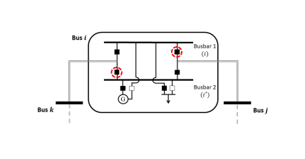
Figure 1: Opening of the circled breakers leads to a bus split event at bus $i$.

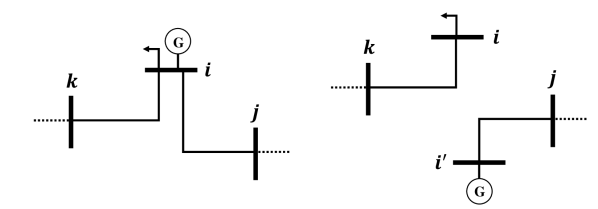
Figure 2: (Left) Original bus-branch model and (right) model with a bus split at bus $i$.

Proposition 1.

Consider the split of bus $i$ with a single line $(i,j)$ and injection $\tilde{p}_{i}$ reconnected to the new bus $i^{\prime}$ (shown in Fig. 2). The post-split system is equivalent to having the opening of line $(i,j)$ and an additional power transfer $\tilde{p}_{i}$ between buses $i$ and $j$.

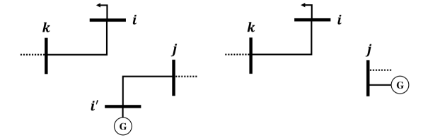
Figure 3: Equivalent reduced bus-branch model (right) for the (left) system with bus split.

The equivalent model for the post-split system is demonstrated in Fig. 3. Because the new bus $i^{\prime}$ connects only to bus $j$, it can be eliminated from the system by moving its connected injection ($\tilde{p}_{i}=g_{i}$ in this generation-only case) directly to bus $j$. Compared to the original system shown in Fig. 2, the equivalent system experiences the opening of line $(i,j)$ in addition to a power transfer of $\tilde{p}_{i}$ between buses $i$ and $j$. This equivalent model has also been verified by linear sensitivity analysis for the bus split events [21]. Proposition 2 is very useful for simplifying the incorporation of bus split events into the topology optimization problem, as discussed in the ensuing section.

III Substation Level Grid Topology Optimization

The grid topology optimization problem aims to determine the optimal transmission grid topology with associated generation outputs in order to minimize the total generation cost. The feasible region of generation dispatch for this problem is the union of the sets of feasible solutions corresponding to each topology configuration. Thus, varying the grid topology will likely expand the overall feasible region and accordingly reduce the total generation costs [2, 3]. Going beyond the traditional topology optimization framework, the inclusion of substation level bus split events allows for additional topology change, and hence it can further reduce grid congestion and improve the security of grid operations.

The nonlinear ac topology optimization formulation is well known to suffer from scalability issues, greatly challenging its real-time implementation [22, 23, 24].

Remark.

In this work, we adopt the dc power flow model for formulating topology optimization problem. The proposed dc based model can be possibly generalized to the nonlinear ac formulation as well; see e.g., [25]. To corroborate the validity of the dc model, we will provide several numerical tests Section IV-B to assert the feasibility of the switching solutions under the ac power flow model.

III-A Modeling of Power Transfer in Bus Splitting

We first discuss different scenarios of generation/load connection for modeling the power transfer in Proposition 2.

Figure 4: Line $\ell=(i,j)$ with connected generation/load for modeling power transfer between buses $i$ and $j$.

To this end, consider a transmission line $\ell=(i,j)$ that connects to buses $i$ and $j$, as shown in Fig. 4. Without loss of generality, the case of having both generation and load is assumed for the two buses. The bus split event can result in a model that is mathematically equivalent to a power transfer in between. For instance, the split of bus $i$ can be associated with one of three power transfer scenarios from bus $i$ to bus $j$, namely load only, generation only, and generation plus load. To represent the change of power injection for all three scenarios, define the following $N\times 3$ matrix:

$$\bm{\Delta}_{\ell,i}(\bm{g})=(\mathbf{e}_{i}-\mathbf{e}_{j})\left[d_{i}\quad-\!g_{i}\quad d_{i}\!-\!g_{i}\right]$$ (5)

where $\mathbf{e}_{i}\in\mathbb{R}^{N\times 1}$ denotes the standard basis vector. Each column of $\bm{\Delta}_{\ell,i}(\bm{g})$ corresponds to one of three aforementioned scenarios under the split of bus $i$. Similarly, one can define this power injection matrix for the split of bus $j$, as:

$${\bm{\Delta}}_{\ell,j}(\bm{g})=(\mathbf{e}_{j}-\mathbf{e}_{i})\left[d_{j}\quad-\!g_{j}\quad d_{j}\!-\!g_{j}\right].$$ (6)

Notice that both $\bm{\Delta}_{\ell,i}(\bm{g})$ and ${\bm{\Delta}}_{\ell,j}(\bm{g})$ depend on the generation output $\bm{g}$, which is a decision variable. In what follows, we use $\bm{\Delta}_{\ell,i}$ to refer to $\bm{\Delta}_{\ell,i}(\bm{g})$ when the dependence on $\bm{g}$ is clear from the context.

III-B Topology Optimization with Bus Splitting

Upon defining the power injection matrices, we are ready to formulate the topology optimization problem that includes the bus split operation. To this end, consider the linear generation cost model, with $\bm{c}\in\mathbb{R}^{N}$ collecting all the linear coefficients. The binary decision variable ${z}_{\ell}$ is introduced for each transmission line $\ell=(i,j)$ to indicate the equivalent line status (1: closed, 0: open), which will be explained in more detail after the formulation. The incident buses for line $\ell$ are collected in the set $\mathcal{N}_{\ell}$. A vector of binary variables $\bm{w}_{\ell,i}\in\{0,1\}^{3}$ is used to select the power transfer scenario in case of a bus split at bus $i$, leading to an equivalent outage on line $\ell=(i,j)$. Similarly, vector ${\bm{w}}_{\ell,j}\in\{0,1\}^{3}$ is defined to select the power transfer scenario in case of a bus split at bus $j$, with an equivalent outage on line $\ell=(i,j)$. Under a maximum budget of $s$ operations (either line switching or bus splitting), one can formulate the following optimization problem:

$$\min\quad {\bm{c}^{\mathsf{T}}\bm{g}}$$ (7a)

over $$\bm{\theta}\in\mathbb{R}^{N},\bm{g}\in\mathbb{R}^{N},\bm{f}\in\mathbb{R}^{L},z_{\ell}\in\{0,1\},\;\forall\ell\in\mathcal{L}$$

$$\bm{w}_{\ell,i}\in\{0,1\}^{3},{\bm{w}}_{\ell,j}\in\{0,1\}^{3},\;\forall\ell=(i,j)\in\mathcal{L}$$

s.t. $${\theta}_{i}^{\min}\leq{\theta}_{i}\leq{\theta}_{i}^{\max},\;\forall i$$ (7b)

$${g}_{i}^{\min}\leq{g}_{i}\leq{g}_{i}^{\max},\;\forall i$$ (7c)

$${f}_{\ell}^{\min}{z}_{\ell}\leq{f}_{\ell}\leq{f}_{\ell}^{\max}{z}_{\ell},\;\forall\ell$$ (7d)

$$b_{ij}(\theta_{i}-\theta_{j})-f_{\ell}+(1-z_{\ell})\mathrm{M}_{\ell}\geq 0,\;\forall\ell=(i,j)$$ (7e)

$$b_{ij}(\theta_{i}-\theta_{j})-f_{\ell}-(1-z_{\ell})\mathrm{M}_{\ell}\leq 0,\;\forall\ell=(i,j)$$ (7f)

$$\sum_{\ell}(1-z_{\ell})\leq s$$ (7g)

$$\bm{1}^{\mathsf{T}}\bm{w}_{\ell,i}+\bm{1}^{\mathsf{T}}{\bm{w}}_{\ell,j}\leq 1-z_{\ell},\;\forall\ell=(i,j)$$ (7h)

$$\sum_{\ell:i\in\mathcal{N}_{\ell}}\bm{1}^{\mathsf{T}}\bm{w}_{\ell,i}\leq 1,\;\forall i$$ (7i)

$$\mathbf{A}\bm{f}\!=\!\bm{g}\!-\!\bm{d}+\!\sum_{\ell=(i,j)}\!\bm{\Delta}_{\ell,i}\bm{w}_{\ell,i}\!+\!\sum_{\ell=(i,j)}\!{\bm{\Delta}}_{\ell,j}{\bm{w}}_{\ell,j}$$ (7j)

$$f_{\ell}^{\min}\bm{1}\!\leq\!\bm{\Delta}_{\ell,i}\bm{w}_{\ell,i}+\!{\bm{\Delta}}_{\ell,j}{\bm{w}}_{\ell,j}\leq f_{\ell}^{\max}\bm{1},\;\forall\ell=(i,j)$$ (7k)

We discuss the constraints for problem (7) here. Phase angle and generation limits are given in constraints (7b) - (7c). Line flow limits are given in (7d), while the flow $f_{\ell}$ is enforced to be zero when the line is open; i.e., $z_{\ell}=0$. Constraints (7e) - (7f) are introduced for establishing the line flow model in (1), with the constant ${\mathrm{M}}_{\ell}$ being sufficiently large. When the line $\ell=(i,j)$ is closed, the two inequalities are equivalent to the dc power flow equation $f_{\ell}=b_{ij}(\theta_{i}-\theta_{j})$. Otherwise, when the line is open $f_{\ell}=0$ [cf. (7d)], the two constraints are guaranteed to be inactive for a large ${\mathrm{M}}_{\ell}$. This is called the Big-M method [26], which is often used to handle constraints with binary variables. For each line $\ell=(i,j)\in\mathcal{L}$, we set:

$$\mathrm{M}_{\ell}\coloneqq b_{ij}\Delta\theta_{ij}^{\max},$$ (8)

where $\Delta\theta_{ij}^{\max}$ is a given upper bound for angle stability. Constraint (7g) limits the total number of operations including both line switching and bus splitting, and constraint (7h) further defines the operations for each line. Specifically, if $z_{\ell}=0$ and $\bm{1}^{\mathsf{T}}\bm{w}_{\ell,i}+\bm{1}^{\mathsf{T}}{\bm{w}}_{\ell,j}=0$, the operation is simply a line switching of $\ell=(i,j)$, i.e., deenergizing the line $\ell=(i,j)$. Otherwise, when $z_{\ell}=0$ but $\bm{1}^{\mathsf{T}}\bm{w}_{\ell,i}+\bm{1}^{\mathsf{T}}{\bm{w}}_{\ell,j}\neq 0$, then one of the power transfer scenarios is selected after opening line $\ell$, making it equivalent to a bus split at either end of line $\ell$. The latter case utilizes the equivalent model of bus split events and does not actually deenergize line $\ell$. Therefore, $z_{\ell}=0$ itself cannot fully indicate the operation type (line switching or bus splitting) and is called the equivalent line status for this reason.

Constraints (7h) - (7k) are introduced specifically for considering bus split events. Constraint (7h) limits the number of power transfers that can be selected for a bus split involving the opening of line $\ell=(i,j)$. When the line is closed ($z_{\ell}=1$), no power transfer is allowed; Otherwise, when the line is open ($z_{\ell}=0$), at most one ($0$ or $1$) power transfer can be made, depending on whether it is line switching or bus splitting. Furthermore, notice that a single bus can be connected to multiple buses, but the power transfer from bus $i$ to other buses can be made only if the bus is split into two bus bars. Once bus $i$ is split for a power transfer with one of its incident buses, no other power transfer can be made with other buses. Therefore, constraint (7i) limits the power transfer from each bus to be at most once due to the physical limit of the substation. Constraint (7j) enforces the network power balance in (2), where the injection also reflects any power transfer made because of the bus split. Last, (7k) guarantees that for the injection reconnected to the new bus $i^{\prime}$, the power flow on that incident line is not violating the transmission limit of line $\ell=(i,j)$ [cf. Fig. 3].

The main challenge of solving (7) lies in the nonlinearity of the constraints. Specifically, constraints (7j) and (7k) are bilinear in the decision variables, due to the multiplication terms, namely $\bm{\Delta}_{\ell,i}(\bm{g})\bm{w}_{\ell,i}$ and ${\bm{\Delta}}_{\ell,j}(\bm{g}){\bm{w}}_{\ell,j}$. To address these terms, we propose to adopt the McCormick relaxation technique [27] to reformulate the problem that is amenable to off-the-shelf MILP solvers. First, rewrite the following multiplication as:

$$\bm{\Delta}_{\ell,i}\bm{w}_{\ell,i} =\bm{\delta}_{d}^{i}\bm{w}_{\ell,i}d_{i}-\bm{\delta}_{g}^{i}\bm{w}_{\ell,i}g_{i}$$ (9)

where vectors $\bm{\delta}_{d}^{i}:=(\mathbf{e}_{i}-\mathbf{e}_{j})\begin{bmatrix}1&0&1\end{bmatrix}$ and $\bm{\delta}_{g}^{i}:=(\mathbf{e}_{i}-\mathbf{e}_{j})\begin{bmatrix}0&1&1\end{bmatrix}$. We define the product of $\bm{w}_{\ell,i}$ and $g_{i}$ as:

$$\bm{y}_{\ell,i}=\bm{w}_{\ell,i}g_{i},\quad\forall\leavevmode\nobreak\ \ell.$$ (10)

Under the bounds $[g_{i}^{\min},g_{i}^{\max}]$ for generation $g_{i}$, the following four linear inequalities hold:

$$\bm{y}_{\ell,i}\geq\bm{w}_{\ell,i}g_{i}^{\min}$$ (11a)

$$\bm{y}_{\ell,i}\geq\bm{1}g_{i}+\bm{w}_{\ell,i}g_{i}^{\max}-\bm{1}g_{i}^{\max}$$ (11b)

$$\bm{y}_{\ell,i}\leq\bm{w}_{\ell,i}g_{i}^{\max}$$ (11c)

$$\bm{y}_{\ell,i}\leq\bm{1}g_{i}+\bm{w}_{\ell,i}g_{i}^{\min}-\bm{1}g_{i}^{\min}.$$ (11d)

The inequalities (11a) - (11d) can be verified by substituting (10). Conversely, for any binary $\bm{w}_{\ell,i}$, the linear inequalities in (11) also guarantee the validity of (10). When the $k$-th entry in the binary $\bm{w}_{\ell,i}$ is equal to zero, the two inequalities (11a) and (11c) jointly force the $k$-th entry of $\bm{y}_{\ell,i}$ to be zero. Otherwise, when the $k$-th entry of $\bm{w}_{\ell,i}$ is equal to one, the inequalities (11b) and (11d) enforce that the $k$-th entry of $\bm{y}_{\ell,i}$ is equal to $g_{i}$. Due to the binary vector $\bm{w}_{\ell,i}$, the set of inequalities in (11) is equivalent to the bilinear relation in (10). Reformulating (10) with the linear inequalities in (11) is known as the McCormick relaxation technique, which has been popularly used in other problems of designing grid topology [28, 29].

Hence, the bilinear product as given in (9) can be equivalently replaced with:

$$\bm{\Delta}_{\ell,i}\bm{w}_{\ell,i}=\bm{\delta}_{d}^{i}\bm{w}_{\ell,i}d_{i}-\bm{\delta}_{g}^{i}\bm{y}_{\ell,i}$$ (12)

and the linear inequality constraints (11a) - (11d). Similarly, the bilinear product of ${\bm{\Delta}}_{\ell,j}$ and ${\bm{w}}_{\ell,j}$ can be directly given as:

$${\bm{\Delta}}_{\ell,j}{\bm{w}}_{\ell,j}=\bm{\delta}_{d}^{j}{\bm{w}}_{\ell,j}d_{j}-\bm{\delta}_{g}^{j}{\bm{y}}_{\ell,j}$$ (13)

for similarly defined $\bm{\delta}_{d}^{j}$ and $\bm{\delta}_{g}^{j}$, together with the following four linear inequalities:

$${\bm{y}}_{\ell,j}\geq{\bm{w}}_{\ell,j}g_{j}^{\min}$$ (14a)

$${\bm{y}}_{\ell,j}\geq\bm{1}g_{j}+{\bm{w}}_{\ell,j}g_{j}^{\max}-\bm{1}g_{j}^{\max}$$ (14b)

$${\bm{y}}_{\ell,j}\leq{\bm{w}}_{\ell,j}g_{j}^{\max}$$ (14c)

$${\bm{y}}_{\ell,j}\leq\bm{1}g_{j}+{\bm{w}}_{\ell,j}g_{j}^{\min}-\bm{1}g_{j}^{\min}.$$ (14d)

Thus, we have reformulated the bilinear products $\bm{\Delta}_{\ell,i}\bm{w}_{\ell,i}$ and ${\bm{\Delta}}_{\ell,j}{\bm{w}}_{\ell,j}$ using linear constraints (12) and (13) followed by additional linear inequalities (11a) - (11d) and (14a) - (14d). Therefore, the equivalent topology optimization problem that incorporates substation bus splitting operation can be established in the following proposition.

Proposition 2.

The original nonlinear optimization problem (7) is equivalent to the following one:

$$\min\quad {\bm{c}^{\mathsf{T}}\bm{g}}$$ (15a)

over $$\bm{\theta}\in\mathbb{R}^{N},\bm{g}\in\mathbb{R}^{N},\bm{f}\in\mathbb{R}^{L},z_{\ell}\in\{0,1\},\;\forall\ell\in\mathcal{L}$$

$$\bm{w}_{\ell,i}\in\{0,1\}^{3},{\bm{w}}_{\ell,j}\in\{0,1\}^{3},\;\forall\ell=(i,j)\in\mathcal{L}$$

$$\bm{y}_{\ell,i}\in\mathbb{R}^{3},{\bm{y}}_{\ell,j}\in\mathbb{R}^{3}\qquad\qquad\ \;\forall\ell=(i,j)\in\mathcal{L}$$

s.t. $$\eqref{eq:TS1_d}-\eqref{eq:TS1_k},\eqref{eq:mci_c}-\eqref{eq:mci_f},\eqref{eq:mcj_c}-\eqref{eq:mcj_f}$$ (15b)

$$\begin{split}&\mathbf{A}\bm{f}=\bm{g}-\bm{d}+\sum_{\ell=(i,j)}(\bm{\delta}_{d}^{i}\bm{w}_{\ell,i}d_{i}-\bm{\delta}_{g}^{i}\bm{y}_{\ell,i})\\ &\quad\qquad+\sum_{\ell=(i,j)}(\bm{\delta}_{d}^{j}{\bm{w}}_{\ell,j}d_{j}-\bm{\delta}_{g}^{j}{\bm{y}}_{\ell,j})\end{split}$$ (15c)

$$\begin{split}f_{\ell}^{\min}\bm{1}&\leq\bm{\delta}_{d}^{i}\bm{w}_{\ell,i}d_{i}-\bm{\delta}_{g}^{i}\bm{y}_{\ell,i}+\bm{\delta}_{d}^{j}{\bm{w}}_{\ell,j}d_{j}\\ &\qquad\qquad\quad-\bm{\delta}_{g}^{j}{\bm{y}}_{\ell,j}\leq f_{\ell}^{\max}\bm{1},\quad\forall\ell=(i,j).\end{split}$$ (15d)

This reformulated problem is a mixed-integer linear program (MILP) and can be efficiently solved by common optimization solvers such as CPLEX, MOSEK and Gurobi. Moreover, since this work directly considers a minimal set of decisions on line switching and power transfer as a result of substation bus splits, the dimension of binary decision variables has been greatly reduced from the original one under the detailed node-breaker representation. This reduction does not affect the solution quality, as one can easily recover the underlying CB status and thus determine the corresponding breaker actions. Therefore, our proposed approach has utilized the concise bus-branch representation to attain an efficient and effective transmission grid switching solution using substation-level actions.

IV Numerical Results

In this section, we first use the IEEE 14-bus system to mainly illustrate that bus split operations can be used to effectively relieve network congestion and to help address feasibility issues of the optimal power flow problem. After that, we perform the substation-level topology optimization on the larger sized IEEE 118-bus system to demonstrate the economic improvement on generation dispatch and to assess the computational complexity of the proposed topology optimization model. The optimization problems have been implemented on a regular laptop with Intel CPU @ 2.60 GHz and 12 GB of RAM in the MATLAB R2018a simulator. The MILP-based optimization problems are computed using the CPLEX solver.

IV-A 14-Bus System Test

The IEEE 14-bus system consists of 20 transmission lines and 5 conventional generators, and we use the ac power flow model to test the system. The system has been slightly modified to illustrate that the bus splitting can be used to relieve network congestion and thus can help with the feasibility issue of the optimal power flow problem. Specifically, we modify the transmission limits of lines $(2,3)$ and $(3,4)$ to be $100$ MW and $10$ MW, respectively. The maximum generation limit of the generator at Bus 3 is adjusted to be $20$ MW, and all other network configurations are kept unaltered.

For Bus 3 in the original system, as shown in Fig. 5, a net load of at least $\bm{d}_{3}-\overline{\bm{g}_{3}}=74.2$ MW needs to be satisfied by the flows from line $(2,3)$ and line $(3,4)$. Due to the electrical characteristics of the lines, power flows on both lines are governed by the phase angle at Bus 3. Therefore, as we gradually increase the flow on line $(2,3)$, the transmission limit on line $(3,4)$ will be eventually violated before the sum of power flows on both lines meets the net load at Bus 3, leading to an infeasible solution to the optimal power flow problem. In order to relieve the congestion on line $(3,4)$ in this scenario, solving the proposed topology optimization problem suggests performing a bus split at Bus 3 such that the generator is connected to bus bar $3^{{}^{\prime}}$ and the load is connected to bus bar $3^{{}^{\prime\prime}}$. Essentially, this bus splitting decouples the power flows on lines $(2,3)$ and $(3,4)$ by allowing each bus bar to have a different phase angle. After the bus splitting, the load at Bus 3 can be easily satisfied by the flow from line $(2,3)$ without violating any transmission limit. Thus, the ac power flow model of the system for the updated system as shown in Fig. 5 becomes feasible. In fact, the bus split operation can be easily achieved through switching associated CBs at the substation. The case study on this small system indicates that similar to traditional line switching and load shedding, the operation of bus splitting can be also used to relieve network congestion and help with feasibility issues. Although the model used in (15) is a dc power flow model, the solution obtained which suggests a bus splitting at Bus 3 makes the problem feasible while considering the ac power flow model. Next, we will use a larger sized system to illustrate the enhanced economic benefit of the proposed substation-level topology optimization algorithm.

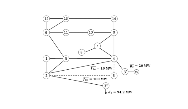
Figure 5: Bus splitting at Bus 3 in the IEEE 14-bus system.

IV-B 118-Bus System Test

The IEEE 118-bus test case is tested for the substation-level topology optimization. The system consists of 118 buses, 186 transmission lines and 19 committed conventional generators. To illustrate the improvement and economic benefits of the topology optimization by incorporating bus split events, we also tested the same system for the traditional topology optimization strategy [2]. This can be easily fulfilled by restricting $\bm{w}_{\ell,i}$ and ${\bm{w}}_{\ell,j}$ in (7) to be zero, which will exclude bus splits from consideration and allow for only line-switching operations. By doing so, constraints (7h), (7i) and (7k) always hold and are thus disabled. Meanwhile, (7j) becomes a linear constraint, which describes the network power balance without any power transfer. Accordingly, the optimization problem (7) itself constitutes an MILP that is readily solvable for common optimization solvers.

The comparison of total cost under different numbers of operations for line switching and breaker-level switching is given in Fig. 6 together with the benchmark cost for the system without any topology switching. Compared with the benchmark cost which involves no topology optimization, our proposed breaker-switching strategy achieves total savings of $14.1\%-23.4\%$, depending on the number of operations; cf. Fig. 6. Meanwhile, compared with line switching, it provides additional cost savings of $4.9\%-7.5\%$ correspondingly. Notice that these additional savings are obtained only by altering the status of several breakers at the substations, therefore the economic benefits are indeed attractive for system operators.

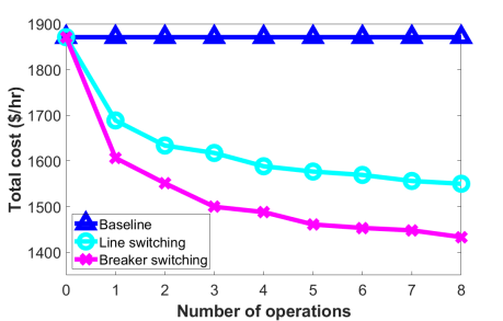
Figure 6: Comparison of total cost between line switching and breaker switching for the 118-bus system.

Table I: Comparison of Topology Optimization Decisions for the 118-Bus System

$s$	Line Switching	Breaker Switching	Reduction
1	Line 128	Bus 82	4.9%
2	Lines 128, 136	Buses 77, 82	5.1%
3	Lines 41, 128, 136	Buses 77, 82 & Line 130	7.3%
4	Lines 119, 123, 124, 125	Buses 75, 77, 82 & Line 136	6.3%
5	Lines 118, 121, 131, 135, 149	Buses 77, 82 & Lines 123, 124, 125	7.3%

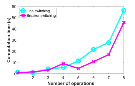
Figure 7: Comparison of computation time between line switching and breaker switching for the 118-bus system.

To compare the switching decisions provided by the traditional line switching and the proposed breaker switching, we list the topology optimization solutions for up to a maximum of $s=5$ operations in Table I. In the line-switching part, only operation on the transmission lines is allowed, which normally involves opening a pair of breakers at both ends of the line. In contrast, the breaker-switching strategy enables more complicated breaker operations that lead to not only line switching but also bus split events. Take $s=3$ as an example, the line-switching scheme picks lines 41, 128 and 136 to open, whereas the proposed breaker switching suggests opening line 130 and performing bus splits at buses 77, 82 simultaneously. As the result of considering breaker-level operations, an additional reduction of $7.3\%$ in the operational cost is achieved.

Additionally, we assessed the computation time for the two formulations of the topology optimization scheme shown in Fig. 7. For up to $s=8$ operations, on average the solving time for the substation-level topology optimization is $28.1\%$ faster than the line-switching one. Notice that compared with the line-switching formulation, we further introduce variables such as $\bm{w}_{\ell,i}$, ${\bm{w}}_{\ell,j}$, ${\bm{y}}_{\ell}$ and ${\bm{y}}_{\ell,j}$, but the additional constraints (7h) - (7i) that incorporate bus split events can potentially facilitate the computation of the resultant MILP problem. In fact, when the number of operations increases, the additional savings on generation cost usually become less significant; cf. Fig. 6. In addition, excessive switching operations can lead to security and stability issues in transmission grids (see e.g.,[2]). Therefore, in practice the number of operations is normally restricted to a small number. In the tested 118-bus system, until $s=5$ operations, the proposed control scheme only requires less than $10$ seconds to find the solution. The results imply the efficiency and scalability of the proposed optimization formulation for real-time implementation.

AC feasibility

It is certainly important to ensure that the switching decisions of the topology optimization problem (15) are feasible considering the ac power model. Thus, we verified the decisions of the breaker-level topology optimization shown in Table I using the ac power flow. Our results confirm that the ac power flow model remains feasible in the post-event systems for the proposed topology optimization.

V CONCLUSIONS

In this paper, we present a post-event analysis of substation bus splits and arrive at an equivalent bus-branch model for such events. Using this equivalent model, we propose a substation-level network topology optimization formulation that can incorporate both line switching and bus splitting. To deal with the bilinearity in the formulation, the McCormick relaxation has been utilized to devise a tractable MILP reformulation, which can be efficiently solved for real-time applications. Numerical studies on the IEEE 118-bus system corroborate the efficacy of the proposed topology optimization algorithm in terms of operational cost reduction and computational complexity. Future work includes topology optimization under an increased set of bus split operations such as the reconnection of multiple lines/injections. To accelerate the running time of ac power flow based topology optimization, we are also interested to explore a learning-based framework to approach the associated mixed-integer program.

References

- [1] A. J. Wood, B. F. Wollenberg, and G. B. Sheblé, Power generation, operation, and control. John Wiley & Sons, 2013.
- [2] E. B. Fisher, R. P. O’Neill, and M. C. Ferris, “Optimal transmission switching,” IEEE Trans. Power Systems, vol. 23, no. 3, pp. 1346–1355, 2008.
- [3] K. W. Hedman, R. P. O’Neill, E. B. Fisher, and S. S. Oren, “Optimal transmission switching with contingency analysis,” IEEE Trans. Power Systems, vol. 24, no. 3, pp. 1577–1586, 2009.
- [4] P. A. Ruiz, J. M. Foster, A. Rudkevich, and M. C. Caramanis, “Tractable transmission topology control using sensitivity analysis,” IEEE Trans. Power Systems, vol. 27, no. 3, pp. 1550–1559, 2012.
- [5] F. Qiu and J. Wang, “Chance-constrained transmission switching with guaranteed wind power utilization,” IEEE Trans. Power Systems, vol. 30, no. 3, pp. 1270–1278, 2015.
- [6] Y. Zhou, H. Zhu, and G. A. Hanasusanto, “Transmission switching under wind uncertainty using linear decision rules,” in Proc. IEEE PES General Meeting, 2020.
- [7] A. A. Mazi, B. F. Wollenberg, and M. H. Hesse, “Corrective control of power system flows by line and bus-bar switching,” IEEE Trans. Power Systems, vol. 1, no. 3, pp. 258–264, 1986.
- [8] W. Shao and V. Vittal, “Corrective switching algorithm for relieving overloads and voltage violations,” IEEE Trans. Power Systems, vol. 20, no. 4, pp. 1877–1885, 2005.
- [9] F. Zaoui, S. Fliscounakis, and R. Gonzalez, “Coupling OPF and topology optimization for security purposes,” in 15th Power Systems Computation Conference, 2005, pp. 22–26.
- [10] M. Heidarifar and H. Ghasemi, “A network topology optimization model based on substation and node-breaker modeling,” IEEE Trans. Power Systems, vol. 31, no. 1, pp. 247–255, 2015.
- [11] Y. Pradeep, P. Seshuraju, S. A. Khaparde, and R. K. Joshi, “CIM-based connectivity model for bus-branch topology extraction and exchange,” IEEE Trans. Smart Grid, vol. 2, no. 2, pp. 244–253, 2011.
- [12] B. Park, J. Holzer, and C. L. DeMarco, “A sparse tableau formulation for node-breaker representations in security-constrained optimal power flow,” IEEE Trans. Power Systems, vol. 34, no. 1, pp. 637–647, 2019.
- [13] B. Park and C. L. Demarco, “Optimal network topology for node-breaker representations with AC power flow constraints,” IEEE Access, vol. 8, pp. 64 347–64 355, 2020.
- [14] G. P. McCormick, “Computability of global solutions to factorable nonconvex programs: Part I-Convex underestimating problems,” Mathematical programming, vol. 10, no. 1, pp. 147–175, 1976.
- [15] V. Kekatos and G. B. Giannakis, “Joint power system state estimation and breaker status identification,” in Proc. North American Power Symp., 2012.
- [16] G. Korres, P. Katsikas, and G. Chatzarakis, “Substation topology identification in generalized state estimation,” International Journal of Electrical Power & Energy Systems, vol. 28, no. 3, pp. 195–206, 2006.
- [17] D. Deka, R. Baldick, and S. Vishwanath, “One breaker is enough: Hidden topology attacks on power grids,” in Proc. IEEE PES General Meeting, 2015.
- [18] C.-W. Ten, K. Yamashita, Z. Yang, A. V. Vasilakos, and A. Ginter, “Impact assessment of hypothesized cyberattacks on interconnected bulk power systems,” IEEE Trans. Smart Grid, vol. 9, no. 5, 2017.
- [19] Y. Zhou, J. Cisneros-Saldana, and L. Xie, “False analog data injection attack towards topology errors: Formulation and feasibility analysis,” in Proc. IEEE PES General Meeting, 2018.
- [20] A. A. Jahromi, A. Kemmeugne, D. Kundur, and A. Haddadi, “Cyber-physical attacks targeting communication-assisted protection schemes,” IEEE Trans. Power Systems, vol. 35, no. 1, pp. 440–450, 2019.
- [21] Y. Zhou and H. Zhu, “Bus split sensitivity analysis for enhanced security in power system operations,” in Proc. North American Power Symp., 2019.
- [22] M. Soroush and J. D. Fuller, “Accuracies of optimal transmission switching heuristics based on DCOPF and ACOPF,” IEEE Trans. Power Systems, vol. 29, no. 2, pp. 924–932, 2013.
- [23] Y. Bai, H. Zhong, Q. Xia, and C. Kang, “A two-level approach to AC optimal transmission switching with an accelerating technique,” IEEE Trans. Power Systems, vol. 32, no. 2, pp. 1616–1625, 2016.
- [24] A. S. Zamzam and K. Baker, “Learning optimal solutions for extremely fast AC optimal power flow,” in 2020 IEEE International Conference on Communications, Control, and Computing Technologies for Smart Grids (SmartGridComm). IEEE, 2020, pp. 1–6.
- [25] B. Kocuk, S. S. Dey, and X. A. Sun, “New formulation and strong MISOCP relaxations for AC optimal transmission switching problem,” IEEE Trans. Power Systems, vol. 32, no. 6, pp. 4161–4170, 2017.
- [26] I. Griva, S. G. Nash, and A. Sofer, Linear and nonlinear optimization. Siam, 2009, vol. 108.
- [27] A. Gupte, S. Ahmed, M. S. Cheon, and S. Dey, “Solving mixed integer bilinear problems using MILP formulations,” SIAM Journal on Optimization, vol. 23, no. 2, pp. 721–744, 2013.
- [28] S. Bhela, D. Deka, H. Nagarajan, and V. Kekatos, “Designing power grid topologies for minimizing network disturbances: An exact MILP formulation,” in Proc. American Control Conference (ACC), 2019.
- [29] M. Bazrafshan, N. Gatsis, and H. Zhu, “Optimal power flow with step-voltage regulators in multi-phase distribution networks,” IEEE Trans. Power Systems, vol. 34, no. 6, pp. 4228–4239, 2019.