Uncertainty Estimation and Sample Selection
for Crowd Counting

Abstract

We present a method for image-based crowd counting, one that can predict a crowd density map together with the uncertainty values pertaining to the predicted density map. To obtain prediction uncertainty, we model the crowd density values using Gaussian distributions and develop a convolutional neural network architecture to predict these distributions. A key advantage of our method over existing crowd counting methods is its ability to quantify the uncertainty of its predictions. We illustrate the benefits of knowing the prediction uncertainty by developing a method to reduce the human annotation effort needed to adapt counting networks to a new domain. We present sample selection strategies which make use of the density and uncertainty of predictions from the networks trained on one domain to select the informative images from a target domain of interest to acquire human annotation. We show that our sample selection strategy drastically reduces the amount of labeled data from the target domain needed to adapt a counting network trained on a source domain to the target domain. Empirically, the networks trained on the UCF-QNRF dataset can be adapted to surpass the performance of the previous state-of-the-art results on NWPU dataset and Shanghaitech dataset using only 17$\%$ of the labeled training samples from the target domain.

Code: https://github.com/cvlab-stonybrook/UncertaintyCrowdCounting

1 Introduction

Crowd counting from unconstrained images is a challenging task due to the large variation in occlusion, crowd density, and camera perspective. Most recent methods [51, 40, 39, 34, 31, 26, 44, 32] learn a Convolutional Neural Network (CNN) to map an input image to the corresponding crowd density map, from which the total count can be computed by summing all the predicted density values at all pixels. Although the performance of the crowd counting methods have improved significantly in the recent years, their performance on the challenging datasets such as [10, 51, 9] is far below the human-level performance. One factor affecting the performance of the existing crowd counting systems is the limited amount of annotated training data. The largest crowd counting dataset [45] consist of 5,109 images. Annotating dense crowd images, which involves placing a dot over the head of each person in the crowd, is time consuming. This makes it harder to create large-scale crowd counting datasets.

(a)

(b)

Figure 1: Different sample selection strategies based on uncertainty estimation. (a) uncertainty based sample selection: Images with higher average uncertainty values are selected for annotation. (b) Ensemble disagreement based sample selection: Given networks A and B trained on a source domain, and a set of unlabeled images from a target domain, we obtain the crowd density map and uncertainty values from both networks for all images in the target domain. Based on the prediction, we compute the disagreement between the two networks. Images with large disagreement are picked for human annotation.

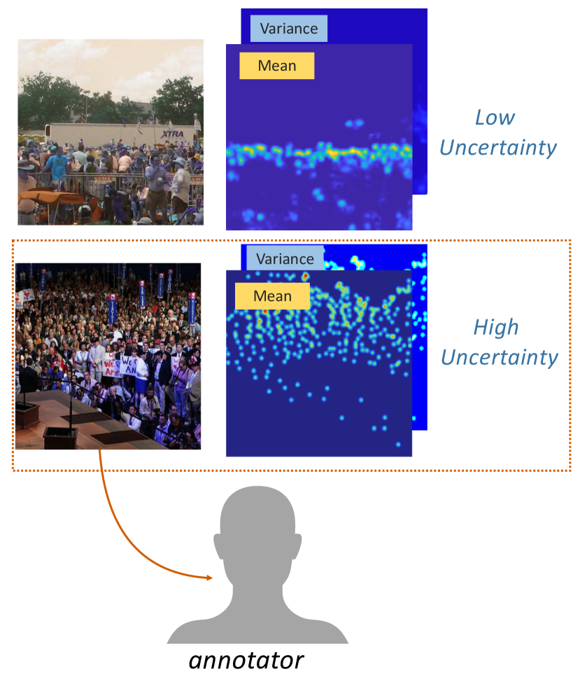
In this paper, we present an approach to tackle the prohibitively large costs involved in annotating crowd images. Our approach draws inspiration from Active Learning, which is based on the hypothesis that a learning algorithm can perform well with less training data if it is allowed to select informative samples [15, 35]. Given a pool of labeled crowd images from the source domain and a large pool of unlabeled crowd images, we are interested in identifying a subset of informative samples from the unlabeled pool, and instead of annotating the whole pool, we obtain the annotation for these selected samples. To find most informative samples from the unlabeled pool, we train networks on the labeled pool first. Next, we select those samples from the unlabeled pool for which the networks are uncertain about their predictions. However, most existing crowd counting methods do not provide any measure of uncertainty for their predictions. We develop a fully convolutional network architecture for estimating the crowd density and the corresponding uncertainty of prediction. For uncertainty estimation, we follow the approach of Nix and Weigand [28] who used a Multi-Layer Perceptron (MLP) to estimate the uncertainty of prediction. This approach assumes that observed output values are drawn from a Gaussian distribution, and the MLP predicts the mean and variance of the Gaussian distribution. The network is trained by maximizing the log likelihood of the data. The variance serves as a measure of uncertainty of the prediction.

Inspired by Nix and Weigand [28], we develop a fully convolutional architecture with a shared trunk for feature extraction and two prediction heads for predicting the crowd density map and the corresponding variance. This network is trained on the source domain by maximizing the log likelihood of the data. We use the predictions from this network, and present two sampling strategies for selecting informative samples from the target domain for human annotation. We present the overview of our sampling strategy in Fig. 1. Our sampling strategy can be used for selecting images from a large pool of unlabeled images, and it can also be used to pick informative crops from an image. Depending on the annotation budget, it might be useful to get partial annotations for an image by picking informative crops from an image and getting human annotations for the informative crops rather than annotating the entire image. We present experiments on image level sample selection and empirically show that the networks trained on UCF-QNRF dataset can be adapted to surpass the performance of the previous state-of-the-art results on NWPU dataset using less than 17$\%$ of the labeled training samples. We also show that the UCF-QNRF pretrained networks can be adapted to perform well on the Shanghaitech dataset as well, with only a third of annotated examples from Shanghaitech dataset. Our results clearly show the usefulness of using our sampling strategy in saving human annotation cost, and it can help reduce human annotation cost involved with annotating large scale crowd datasets. Our sampling strategy isn’t specific to crowd counting, and it can be applied to any other pixel level prediction task such as optical flow estimation, semantic segmentation as well. We decide to focus on Crowd Counting in this paper since human annotation is particularly expensive for Crowd Counting.

The main contributions of our work are: (1) We propose a novel network architecture for crowd density prediction and corresponding uncertainty estimation that uses both local features and self-attention based non-local features for prediction. (2) We show that modeling prediction uncertainty leads to a more robust loss function, which outperforms the commonly used mean squared loss, obtaining state of the art results on multiple crowd counting datasets. (3) We present a novel uncertainty guided sample selection strategy that enables using networks trained on one domain to select informative samples from another domain for human annotation. To the best of our knowledge, ours is the first work focusing on using predictive uncertainty for sample selection pertaining to any pixel level prediction task in Computer Vision. We show empirically that using the proposed sampling strategy, it is possible to adapt a network trained on a source domain to perform well on the target domain using significantly less annotated data from the target domain.

2 Related Work

Crowd counting is an active area of research with two general approaches: detection approach and density estimation approach. Despite lots of related works, none of them use non-local features to reduce the ambiguity of the estimation, nor use the uncertainty estimates for sample selection.

Detection and Regression Based Approaches. Crowd counting has been studied for a long time. Initial crowd counting approaches [19, 16] were based on detection, which used a classifier such as SVMs trained on top of hand crafted feature representation. These approaches performed well on simpler crowd counting datasets, but their performance was severely affected by occlusion, which is quite common in dense crowd datasets. Some of the later approaches [4, 5] tried to tackle the occlusion problem by avoiding the detection problem, and directly learning a regression function to predict the count.

Density Estimation Based Approaches. The precursor to the current density estimation based approaches was the work of Lempitsky and Zisserman [14], who presented one of the earliest works on density estimation based crowd counting. In the recent deep learning era, density estimation has become the de facto strategy for most of the recent crowd counting approaches  [51, 34, 17, 30, 31, 10, 3, 26, 44, 23, 37, 24, 22, 46, 6, 21, 47, 52, 50, 12, 43, 18, 20, 25].

Starting with Zhang et al. [51], many approaches [2, 31, 40] used multiple parallel feature convolutional columns to extract features at different resolution. Zhang et al. [51] used a multi-column architecture comprising of three columns to address the large variation in crowd size and density. The different columns had kernels of varying sizes. The column with larger kernels could extract features for less dense crowd, while the column with finer kernels is for denser crowd. Sam et al. [34] proposed to decouple different columns, and train them separately. Each column was specialized towards a certain density type. This made the task of each regressor easier, since it had to handle similar density images. They also trained a switch classifier which routed an image patch to the appropriate regressor. However, unlike [51], the training procedure comprised of multiple stages. Sindagi and Patel [40] presented an approach which utilized local and global context information for crowd counting. They trained a classifier for classifying an image into multiple density categories, and the classifier score was used to create context feature maps. Ranjan et al. [31] used a two stage coarse to fine approach to predict crowd density map. In the first stage, a low resolution density map was predicted, which was later utilized as a feature map while predicting the final high resolution density map.

Uncertainty Estimation For Computer Vision tasks, we typically consider two types of uncertainty: aleatoric and epistemic [13]. Aleatoric uncertainty captures the uncertainty inherent in the data, and can be modeled by predicting the parameters of a Gaussian distribution and maximizing the log likelihood [28, 13] of the observed data. Epsitemic uncertainty, also called model uncertainty, is related to the uncertainty in the model parameters, and can be explained away given a large enough dataset. Epistemic uncertainity can be captured by Bayesian Neural Networks [27]. Although performing inference with earlier Bayesian Neural Networks was inefficient, recent techniques like Monte Carlo Dropout [7] can be used to capture epistemic uncertainty even with large neural networks. Some of the earlier works have focused on uncertainty prediction for tasks such as optical flow estimation [11] and crowd counting [29]. However, none of these earlier works have focused on using uncertainty estimates for sample selection.

3 Uncertainty Estimation for Crowd Counting

We take motivation from earlier work Kendall and Gal [13] which shows the usefulness of both Aleatoric and Epistemic Uncertainty estimates for various Computer Vision tasks, and present architectures which can be used for obtaining the two types of uncertainties. In Sec. 3.1, we present our proposed network architecture for estimating the aleatoric uncertainty, followed by training objective in Sec. 3.2.

3.1 Crowd Transformer Network

In this section, we describe our Crowd Transformer Network (CTN) architecture, which predicts the crowd density map along with the corresponding uncertainty values. CTN models the predictive uncertainty, i.e., the uncertainty inherent in the input image which might arise from sensor noise, or from the ambiguity in the image itself.

The block diagram of CTN is presented in Fig. 2. CTN uses both local and non-local features for estimating the crowd density map. Let $X$ be a crowd image of size $H{\times}W$ and $Y$ the corresponding ground truth density map of the same size. We assume that each value in $Y$ is generated by a Gaussian distribution, and CTN predicts the mean and the variance of the Gaussian distribution. The proposed CTN takes input $X$ and predicts mean and variance maps as:

$$X\rightarrow\mu(X,\theta),\sigma^{2}(X,\theta)$$ (1)

where $\mu(X,\theta)$ is the crowd density map and $\sigma^{2}(X,\theta)$ the uncertainty map. We use uncertainty and variance interchangeably in the rest of the paper. Both $\mu(X,\theta)$ and $\sigma^{2}(X,\theta)$ have the same size as the input image $X$ as well as the crowd density map $Y$. The key components of CTN architecture are: 1) a local feature block, 2) a non-local feature block, 3) a density prediction branch, and 4) a uncertainty prediction branch. These components are described below.

Figure 2: CTN architecture predicts both crowd density map and corresponding uncertainty values. It combines local and non-local features. The local features are computed by the convolution layers in the local feature block. The resulting feature map is passed to the non-local feature block. Both density prediction branch and uncertainty prediction branch utilize local and non-local features.

Local Feature Block. Given an input image $X$ of size $H{\times}W$, we pass it through a local feature block to obtain the convolutional feature maps. The local feature block consists of five convolution layers with kernels of size $3{\times}3$, and the number of filters in the convolution layers are 64, 64, 128, 128, and 256. We use the VGG16 network [38] pretrained on ImageNet to initialize the convolution layers in the local feature block. The local feature block has two max pooling layers, after the second and fourth convolution layers. The resulting feature map is a tensor of size $\frac{H}{4}{\times}\frac{W}{4}{\times}256$. The feature map is passed to the non-local block as well as the density prediction branch and uncertainty branch.

Non-local Feature Block. For computing the non-local features, we use the Transformer architecture [42] which was proposed as an alternative to recurrent neural network [33] for solving various sequence analysis tasks. It uses an attention mechanism to encode non-local features. The architecture consists of an encoder and a decoder, where the encoder maps the input sequence into an intermediate representation, which in turn is mapped by the decoder into the output sequence. The transformer uses three types of attention layers: encoder self-attention, encoder-decoder attention, and decoder self-attention. For the proposed crowd counting approach in this paper, only the first one is relevant which we describe briefly next. Henceforth, we will use self-attention to refer to the self-attention of the encoder.

Encoder Self-Attention. Given a query sequence along with a key-and-value sequence, the self-attention layer outputs a sequence where the $i$-th element in the output sequence is obtained as a weighted average of the value sequence, and the weights are decided based on the similarity between the $i$-th query element and the key sequence. Let $X\in R^{n\times d}$ be a matrix representation for a sequence consisting of $n$ vectors of $d$ dimensions. The self-attention layer first transforms $X$ into query $X_{Q}$, key $X_{K}$, and value $X_{V}$ matrices by multiplying $X$ with matrices $W_{Q}$, $W_{K}$, and $W_{V}$, respectively:

$$X_{Q}=XW_{Q},X_{K}=XW_{K},X_{V}=XW_{V}.$$ (2)

The output sequence $Z$ is computed efficiently with matrix multiplications:

$$Z=softmax(X_{Q}X_{K}^{T})X_{V}.$$ (3)

The encoder consists of multiple self-attention layers, arranged in a sequential order so that the output of one layer is fed as input to the next layer.

Architecture Details. The non-local feature block takes as input the feature map from the local feature block, and passes it through three convolution layers of kernel size $3{\times}3$ and a max pooling layer, which results in a feature map of size $\frac{H}{8}{\times}\frac{W}{8}{\times}512$. We reduce the depth of the feature map by passing it through a $1{\times}1$ convolution layer, which yields a feature map of size $\frac{H}{8}{\times}\frac{W}{8}{\times}240$. The resulting feature map is flattened into a matrix of size $M{\times}240$, where $M=\frac{H}{8}{\times}\frac{W}{8}$. Each row in this matrix corresponds to some location in the convolution feature map. The flattened matrix is passed through three self-attention layers. The output from final transformer layer is reshaped back into a tensor of size $\frac{H}{8}{\times}\frac{W}{8}{\times}240$.

Density Prediction Branch. Both local and non-local features are important for estimating an accurate crowd density map. Hence, the Density Prediction Branch uses a skip connection to obtain the convolutional features from the local feature block, and combines it with the features from the non-local feature block. The non-local features are upsampled to the same spatial size as local features, which results in a tensor of size $\frac{H}{4}{\times}\frac{W}{4}{\times}240$. The local and non-local features are concatenated and passed through four convolution layers (with 196, 128, 48, and 1 filters), where the last layer is a $1{\times}1$ convolution layer. We add a ReLU non-linearity after the $1{\times}1$ convolution layer to prevent the network from predicting negative density values. We use two bilinear interpolation layers, after the second and third convolution layers in the prediction head. Each interpolation layer upsamples its input by the factor of two. The input to the final $1{\times 1}$ convolution layer is a feature map of size $H{\times}W{\times}48$, which is transformed into a 2D map by the last convolution layer.

Predictive Uncertainty Estimation Branch. The Predictive Uncertainty Estimation Branch outputs the variance map $\sigma^{2}(X,\theta)$. Similar to the density prediction branch, the uncertainty branch also uses both the local and non-local features for prediction. The uncertainty prediction branch has the same architecture as the density prediction branch, with one major difference being that we use point-wise softplus nonlinearity instead of ReLU nonlinearity after the last $1{\times}1$ convolution layer. Softplus nonlinearity can be expressed as: $softplus(x)=\frac{1}{\beta}\log(1+\exp(\beta x))$. For brevity, we will refer to this type of uncertainty estimation as Predictive Uncertainty.

3.2 Training Objective

The network is trained by minimizing the negative conditional log likelihood of the observed ground truth density values $Y$, conditioned on the input image $X$:

$$\mathcal{L}(Y|X,\theta)=-\sum_{i=1}^{HW}\log(\mathbb{P}(Y_{i}|\mu_{i}(X,\theta),\sigma_{i}^{2}(X,\theta))),$$ (4)

where $\mathbb{P}(y|\mu,\sigma^{2})=\frac{1}{\sqrt{2\pi\sigma^{2}}}\exp(-\frac{(y-\mu)^{2}}{2\sigma^{2}})$, a univariate Gaussian distribution. The negative conditional log likelihood is proportional to:

$$\mathcal{L}(Y|X,\theta)\propto\sum_{i=1}^{HW}\left(\log{\sigma_{i}(X,\theta)}+\frac{(Y_{i}-\mu_{i}(X,\theta))^{2}}{2\sigma^{2}_{i}(X,\theta)}\right).$$

The above objective can be seen as a weighted sum of the squared differences, where the weights depend on the estimated uncertainty of the input $X$. This objective can be seen as a robust regression objective, where higher importance is given to pixels with lower ambiguity [28].

4 Uncertainty Guided Sample Selection

Given a labeled dataset $\{(X_{A},Y_{A})\}$ from domain $A$, and an unlabeled dataset $\{X_{B}\}$ from domain $B$, we are interested in finding a small subset of informative samples from domain $B$. Each instance $X_{B}$ of domain $B$ can be sent to an oracle (human) to obtain the label $Y_{B}$. Our motivation behind selecting a small subset from domain $B$ is to reduce the human annotation cost without sacrificing the performance on domain $B$. Next, we propose different strategies for selecting informative samples. In Sec. 4.1, we propose to use the aleatoric uncertainty predicted by CTN to select informative samples. In Sec. 4.2, we draw inspiration from Query-by-committee [35] sampling strategies in Active Learning, and present a sampling strategy that uses the disagreement between the members of an ensemble of CTN networks for selecting informative samples. We present two strategies for computing the disagreement, the first one uses both the density and the uncertainty predictions while the other uses just the density prediction.

4.1 Aleatoric Uncertainty Based Sample Selection

When picking samples from the target domain, we want to select those samples for which the network makes erroneous prediction. Previous works and our own experiments show that aleatoric uncertainty is correlated to the prediction error (see supplementary materials and Fig. 3). Hence, we propose to use the aleatoric uncertainty for selecting informative samples. We use the CTN network trained on the source domain to compute the aleatoric uncertainty (averaged across the image) for all the images in the target domain, and select those samples from the target domain for labeling that have a high average aleatoric uncertainty.

4.2 Ensemble Disagreement based Sample Selection

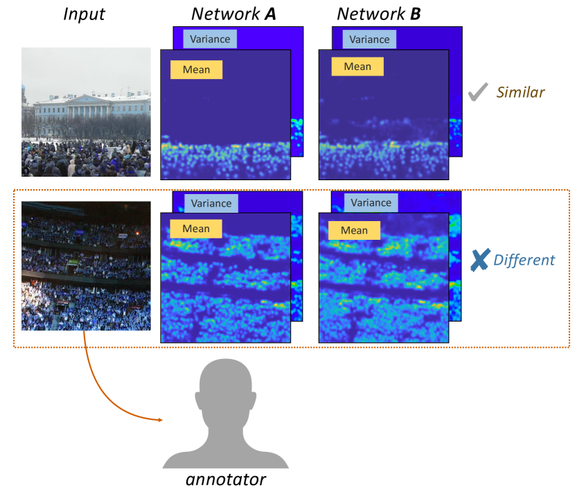
Inspired by the Query-By-Committee [36] sampling algorithm in Active Learning, we present another sampling strategy which uses the predictions from our CTN network trained on a source domain to select informative samples from a target domain. The Query-By-Committee algorithm keeps a committee of students, and picks the sample with maximal disagreement between the committee members to acquire annotation. In this work, the committee is a set of two CTN networks as described in the previous section. These networks are trained on different subsets of labeled data from domain A, and the disagreement between the two networks are used as a measure of informativeness. Let the two networks be represented by their parameters $\theta_{1}$ and $\theta_{2}$ and the outputs of the networks are the mean and variance maps:

$$\left[\mu(X,\theta_{1}),\sigma^{2}(X,\theta_{1})\right]\ \textrm{and }\left[\mu(X,\theta_{2}),\sigma^{2}(X,\theta_{2})\right].$$ (5)

The values $\mu_{i}(X,\theta_{1})$ and $\sigma_{i}^{2}(X,\theta_{1})$ are the mean and variance of a Gaussian distribution for the density value at pixel $i$. Similarly, the values $\mu_{i}(X,\theta_{2})$ and $\sigma_{i}^{2}(X,\theta_{2})$ correspond to another Gaussian distribution. We use the KL divergence between these two distributions as a measure of disagreement between the two density estimation networks. We denote the KL divergence at location $i$ of image $X$ as $KL(X_{i})$, which can be computed in close form as:

$$KL(X_{i})= \frac{\sigma_{i}^{2}(X,\theta_{1})+(\mu_{i}(X,\theta_{1})-\mu_{i}(X,\theta_{2}))^{2}}{2\sigma_{i}^{2}(X,\theta_{2})}+\log\left(\frac{\sigma_{i}(X,\theta_{2})}{\sigma_{i}(X,\theta_{1})}\right)-\frac{1}{2}\cdot$$ (6)

The overall informativeness of an image is obtained by computing the average KL divergence over all pixels. We sort all the images in domain B according to their informativeness, and select the most informative samples for annotation. Note that this approach can be easily extended for more than two networks.

We present another strategy called Density-difference based Ensemble disagreement to compute the disagreement between the members of an ensemble. This disagreement is computed by averaging the pixel wise squared difference between the the density maps predicted by the members of the ensemble as

$$Diff(X_{i})=(\mu_{i}(X,\theta_{1})-\mu_{i}(X,\theta_{2}))^{2}.$$ (7)

The informativeness score is obtained by averaging $Diff(X_{i})$ over the entire prediction map. The score can be generalized to work with an ensemble of multiple networks.

5 Experiments

We validate the proposed approach by conducting experiments on four publicly available datasets: UCF-QNRF [10], UCF CC [9], Shanghaitech [51] and NWPU [45]. In Sec. 5.1, we discuss the crowd counting results on all datasets. Note that we use the entire training set from each dataset for this experiment. In Sec. 5.2, we show the effectiveness of the proposed sample selection strategies. Following previous works, we report Mean Absolute Error (MAE) and Root Mean Squared Error (RMSE) metrics:

$$MAE=\frac{1}{n}\sum_{i=1}^{n}\lvert C_{i}-\hat{C}_{i}\rvert;RMSE=\sqrt[]{\frac{1}{n}\sum_{i=1}^{n}(C_{i}-\hat{C}_{i})^{2}},$$

where $C_{i}$ is the ground truth count, $\hat{C}_{i}$ is the predicted count, and the summation is computed over all test images.

5.1 Crowd Density Prediction

5.1.1 Experiments on UCF-QNRF dataset.

The UCF-QNRF dataset [10] consists of 1201 training and 334 test images of variable sizes, with 1.2 million dot annotations. For our experiments, we rescale those images for which the larger side is greater than 2048 pixels to 2048. For training, we take random crops of size $512{\times}512$ from each image. Keeping the variance prediction branch fixed, we first train the other blocks of the proposed network for 20 epochs using the mean squared error loss. Next, we train only the uncertainty variance prediction head by minimizing the negative log likelihood objective for five epochs. Finally, we train the entire network by minimizing the negative log likelihood for 10 more epochs, and report the best results. We use a learning rate of $10^{-4}$, and a batch size of three for training.

Comparison with existing approaches. Tab. 1 shows the performance of various approaches on the UCF-QNRF dataset. Bayesian Loss [26] is a novel loss function for training crowd counting networks. It outperforms mean squared error, and it has the current state-of-the-art performance. This loss function is complimentary to what we propose here, and it can be used together with CTN. In fact, the method CTN^∗ displayed in Tab. 1 is the combination of CTN and Bayesian Loss. CTN^∗ improves the performance of Bayesian Loss [26] and advances the state-of-the-art result on this dataset.

Ablation Study. The proposed CTN consists of three main components: Local Feature Block, Non-Local Feature Block, and Predictive Uncertainty Estimation Branch. To further understand the contribution of each component, we perform an ablation study, and the results are shown in Tab. 2. As can be seen, all constituent components of CTN are important for maintaining its good performance on the UCF-QNRF dataset.

	UCF-QNRF		NWPU
	MAE	RMSE	MAE	RMSE
Idrees et al. [9]	315	508	-	-
MCNN [51]	277	426	219	701
CMTL [39]	252	514	-	-
Switch CNN  [2]	228	445	-	-
Composition Loss-CNN [10]	132	191	-	-
CSR net [17]	-	-	105	433
CAN  [23]	107	183	94	490
SFCN  [44]	102	171	-	-
ANF [48]	110	174	-	-
Bayesian Loss [26]	89	155	93	470
SCAR [8]	-	-	82	398
CTN∗ (Proposed)	86	146	78	448

Table 1: Performance of various methods on the UCF-QNRF test dataset and NWPU validation dataset. Bayesian Loss is a recently proposed novel loss function for training a crowd counting network. CTN^∗ is the method that combines CTN and Bayesian Loss, advancing the state-of-the-art performance in both MAE and RMSE metrics. Following  [26], we use the first four blocks from Vgg-19 as the backbone for local feature extraction.

Components	Combinations
Local features	✓	✓	✓
Non-Local features	✓	✓		✓
Predictive Uncertainty	✓
MAE	93	106	120	123
RMSE	166	185	218	206

Table 2: Ablation study on UCF-QNRF. CTN is the proposed counting network that consists of: Local Feature Block, Non-local Feature Block, and Uncertainty Prediction Branch. All three components are important for maintaining the good performance of CTN on this dataset. Note that ablation study is done using the Vgg-16 backbone.

Experiments on NWPU-Crowd dataset. NWPU [45] is the largest crowd counting dataset comprising of 5,109 crowd images taken from the web and video sequences, and over $2.1$ million annotated instances. The ground truth for test images are not available, here we present the results on the validation set of NWPU in Tab. 1. For this experiment, we use the pretrained CTN model from UCF-QNRF dataset and adapt the network on the NWPU dataset. Our proposed approach outperforms the previous methods.

Experiments on UCF-CC dataset. The UCF-CC dataset [9] consists of 50 images collected form the web, and the count across the dataset varies between 94 and 4545. We use random crops of size $\frac{H}{3}{\times}\frac{W}{3}$ for training. Following previous works, we perform 5-fold cross validation and report the average result in Tab. 3. The proposed CTN with the Predictive Uncertainty (CTN) is comparable to other state-of-the-art approaches in both MAE and RMSE metrics. For all the approaches, the error on UCF CC dataset is higher compared to the other datasets since it has a small number of training samples.

	UCF-CC		Shtech Part A		Shtech Part B
	MAE	RMSE	MAE	RMSE	MAE	RMSE
Crowd CNN [49]	-	-	181.8	277.7	32.0	49.8
MCNN [51]	377.6	509.1	110.2	173.2	26.4	41.3
Switching CNN [34]	-	-	90.4	135.0	21.6	33.4
CP-CNN [40]	295.8	320.9	73.6	106.4	20.1	30.1
IG-CNN [1]	291.4	349.4	72.5	118.2	13.6	21.1
ic-CNN [31]	260.9	365.5	68.5	116.2	10.7	16.0
SANet  [3]	258.4	334.9	67.0	104.5	8.4	13.6
CSR Net  [17]	266.1	397.5	68.2	115.0	10.6	16.0
PACNN  [37]	241.7	320.7	62.4	102.0	7.6	11.8
SFCN  [44]	214.2	318.2	64.8	107.5	7.6	13.0
ANF [48]	250.2	340.0	63.9	99.4	8.3	13.2
Bayesian Loss [26]	229.3	308.2	62.8	101.8	7.7	12.7
CTN (proposed)	210.0	305.4	61.5	103.4	7.5	11.9

Table 3: Count errors of different methods on the UCF-CC dataset and Shanghaitech dataset. This dataset has two parts: Part A was collected from the web, and Part B was collected from the streets of Shanghai. The average ground truth crowd count for Part A is larger than that for Part B. We report both MAE and RMSE metrics.

Experiments on Shanghaitech dataset. The Shanghaitech dataset [51] consists of two parts. Part A contains 482 images collected from the web, and Part B contains 716 images collected on the streets of Shanghai. The average ground truth crowd counts for Part A and Part B are 501 and 124, respectively. For training, we use random crops of size $\frac{H}{3}{\times}\frac{W}{3}$. Results are shown in Tab. 3. The proposed approach outperforms all existing approaches in terms of MAE. Part A is more challenging with denser crowds than Part B. As a result, the average error of all the approaches on Part A is larger than those on Part B. Note that the CTN network in Tab. 3 is first trained on UCF-QNRF and later finetuned on Shanghitech dataset. This may not be a fair comparison for those approaches in Tab. 3 where the networks are trained from scratch on Shanghaitech dataset. Hence, for a more fair comparison, we train the current state of the art model [26] on UCF-QNRF dataset first, and finetune it on Shanghaitech Part A dataset. We use the official implementation by the authors and use the hyper parameters reported by the authors [26]. This results in MAE/RMSE of 63.4/107.9 on the test set of ShanghaiTech Part A. Our CTN outperforms [26] in this experiment, with MAE/RMSE of 61.5/103.4 reported in Tab. 3. This is a fair comparison since both methods are pretrained on UCF-QNRF, and later finetuned on Shanghaitech Part A.

	Shtech Part A			NWPU
Selection approach	#Train	MAE	RMSE	#Train	MAE	RMSE
None (Pretrained)	NA	69.2	113.5	NA	118.4	632.3
Random	50	68.7	117.1	100	117.4	640.7
Count	50	67.3	107.4	100	107.9	458.8
Aleatoric Uncertainty	50	62.9	108.1	100	104.9	522.1
Density based Ensemble Disagr.	50	61.4	105.5	100	112.8	526.8
KL-Ensemble Disagreement	50	65.5	118.4	100	105.8	481.9
Random	100	65.5	125.5	500	96.7	539.4
Count	100	63.3	109.8	500	95.9	442.5
Aleatoric Uncertainty	100	64.7	107.8	500	81.5	313.7
Density based Ensemble Disagreement	100	62.2	109.6	500	90.0	438.6
KL-Ensemble Disagreement	100	62.1	103.3	500	95.6	511.3
Full dataset (previous best methods)	300	62.8	99.4	3109	82	398
Full dataset (CTN)	300	61.5	103.4	3109	78.1	448.2

Table 4: Comparing different strategies for selecting images for annotation. We train the network on the UCF-QNRF dataset, and use it to select images from the NWPU and Shanghaitech train data for acquiring annotation. We compare the random selection baseline with the proposed uncertainty-guided selection strategy. For NWPU dataset, using just 500 training samples selected using our sampling strategy, we achieve state-of-the-art results compared to the previous state-of-art [8] trained on entire training set in terms of MSE. For Shanghaitech Part A, using just 50 labeled training samples, selected using our density based ensemble disagreement sampling strategy, we perform comparably to the state-of-the-art networks trained on the entire training set.

Image	Ground truth	Mean	Variance	Error
	382	380	0.61	2
	346	329	0.4	17
	282	404	1.01	122

Figure 3: Qualitative Results. This figure shows Image, Ground truth, Predicted Mean, Predicted Variance, and Error map. We specify the sum of the map below the corresponding map. The first two examples are success cases for density estimation, while the last is a failure cases. The variance maps correlate with the error maps.

5.2 Uncertainty Guided Image Annotation

In this section, we evaluate the effectiveness of the proposed selective annotation strategy. We train the network on the UCF-QNRF dataset and use it to select the informative samples from the Shanghaitech Part A dataset and NWPU dataset for acquiring annotation (results on Shanghaitech Part B are presented in the Supplementary). We use the labels of the selected samples, keep the variance prediction branch frozen, and finetune CTN using the selected subset. We compare our sampling approach with two baseline sampling approaches: 1) random sampling approach: images are randomly sampled from the unlabeled pool in the target domain, and 2) Count based sampling: we select those samples from the target domain for which the pretrained network predicts a high count. We report the results in Tab. 4. Note that the entire training sets of Shanghaitech Part A and NWPU have 300 and 3109 images respectively. Our sampling approaches outperform the random baseline by a large margin. We also outperform the Count based sampling baseline. For NWPU dataset, using just 500 training samples, we achieve state-of-the-art results compared to the previous state-of-art [8] trained on the entire training set in terms of MSE. For Shanghaitech Part A, using just 50 labeled training samples, selected using our density based ensemble disagreement sampling strategy, we perform comparably to the state-of-the-art networks trained on the entire training set. Our results clearly show the usefulness of our informative sample selection strategy for transferring counting networks from one domain to another.

5.3 Qualitative Results

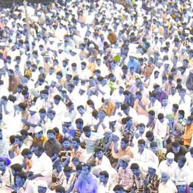
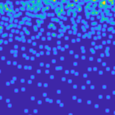
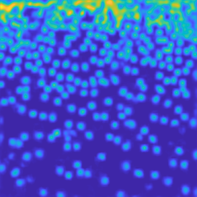
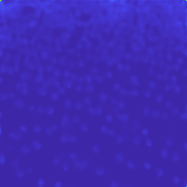
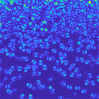
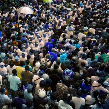
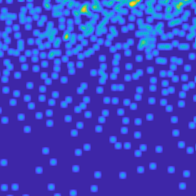
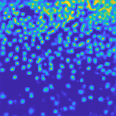
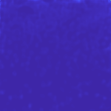
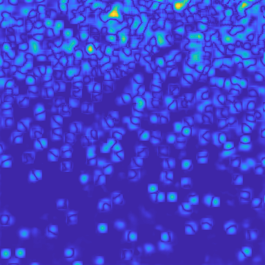
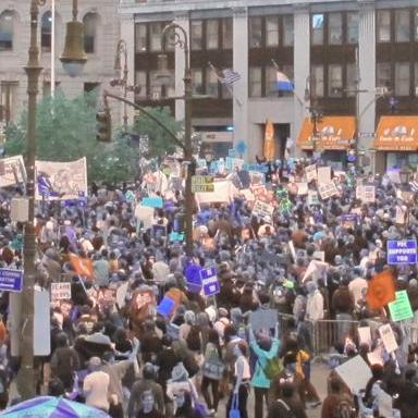
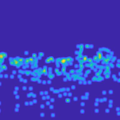
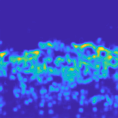
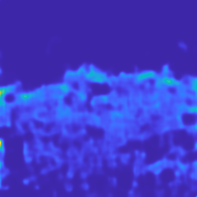
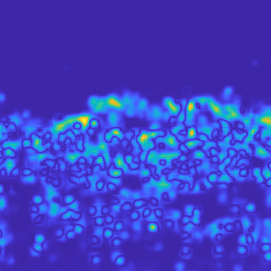
Fig. 3 displays some qualitative585 results from UCF-QNRF dataset. Error is correlated with the variance which suggests the appropriateness of using the variance maps for estimating the uncertainty of the density prediction.

6 Conclusions

To tackle large human annotation costs involved with annotating large scale crowd datasets, we have presented uncertainty based and ensemble disagreement based sampling strategies. These strategies were shown to be useful for the task of transferring a crowd network trained on one domain to a different target domain. Using just $17\%$ of the training samples obtained using our sampling strategy, we obtained state-of-the-art results on two challenging crowd counting datasets. We also showed that our proposed architecture, when trained on the full dataset, achieved state-of-the-art results on all the datasets in terms of mean absolute error.

Acknowledgements: This project is partially supported by MedPod and the SUNY2020 Infrastructure Transportation Security Center.

7 Supplementary Materials

7.1 Overview

Earlier works [13] have shown the usefulness of both Aleatoric and Epistemic Uncertainty estimates for various Computer Vision tasks. In the main paper, we presented our CTN architecture for estimating aleatoric uncertainty pertaining to crowd density prediction. In Sec. 7.2, we present Monte Carlo CTN (MC-CTN), our architecture for estimating epistemic uncertainty. Subsequently in Sec. 7.3, we compare epistemic and aleatoric uncertainty estimates, and show that aleatoric uncertainty is more correlated with the prediction error. In the main paper, we focused on using aleatoric uncertainty estimates for sample selection since our preliminary experiments showed Aleatoric uncertainty to be more effective at sample selection compared with epistemic uncertainty.

In the main paper, we pointed out that our sampling strategy can be used for picking out images from a large pool of unlabeled images, and it can also be used to pick out informative crops from an image. Depending on the annotation budget, it might be useful to get partial annotations for an image by picking out informative crops from an image and getting human annotations for the informative crops rather than annotating the entire image. The experiments on image level sample selection are discussed in the main paper. In Sec. 7.4, we present experiments pertaining to selecting most informative crops from an image for human annotation.

Finally, for image level sample selection, in addition to experiments performed on Shanghaitech Part A [51] and NWPU [45] datasets as shown in the main paper, we present more experiments on Shanghaitech Part B in Sec. 7.5.

Figure 4: The sparsification plots for aleatoric (left) and epistemic (right) uncertainty estimation on the test set of Shanghaitech Part A. The closer the uncertainty curve to the oracle, the higher the correlation between the uncertainty and prediction error. The area between the uncertainty curve and the oracle curve for the two cases is 0.07 and 0.25. The aleatoric uncertainty is more correlated with the prediction error.

7.2 Epistemic Uncertainty Estimation

The CTN architecture described in the main paper captures the aleatoric uncertainty, i.e., the uncertainty inherent in the input data. In this section, we present a variant of CTN which can capture the model uncertainty, which is also known as Epistemic Uncertainty and arises due to the use of finite training data. Epistemic uncertainty, can be captured by Bayesian Neural Networks [27]. Such networks assume a prior distribution $\mathbb{P}(\theta)$ over the parameters of the network, and find the posterior probability $\mathbb{P}(\theta|\{X,Y\})$ conditioned on the training data $\{X,Y\}$. However, it is computationally expensive to perform inference with Bayesian Neural Networks with large number of parameters. To address this issue, [7] present a variational approximation which corresponds to adding a dropout [41] layer before every weight layer. The uncertainty in such a network can be obtained by doing multiple forward passes of the input image through the network, and computing the sample mean as the prediction output. The sample variance is the epistemic uncertainty of the prediction. This approach requires running the network multiple times with different dropout instantiations, so we will refer to it as Monte Carlo Uncertainty.

We will refer to a counting network where Predictive Uncertainty is replaced by Monte Carlo Uncertainty as Monte Carlo CTN (MC-CTN). MC-CTN is similar to CTN presented in the main paper with two major differences: 1) we remove the Predictive Uncertainty Estimation branch, and 2) we add a dropout layer before every convolution layer except for the ones in density prediction branch.

Performance of MC-CTN on Crowd Counting MC-CTN led to MAE/RMSE of 102/180 on UCF-QNRF dataset. CTN, as reported in the main paper, outperforms MC-CTN and results in MAE/RMSE of 86/146.

	Shtech Part A
Selection approach	#Crops	MAE	RMSE
None (Pretrained)	NA	69.2	113.5
Random	1 of 16	68.6	113.5
Count	1 of 16	68.2	113.9
Aleatoric Uncertainty	1 of 16	65.7	103.5
Density based Ensemble Disagre.	1 of 16	66.4	112.4
KL-Ensemble Disagreement	1 of 16	66.4	109.7
Full dataset (previous best method)	full image	62.8	99.4
Full dataset (CTN)	full image	61.5	103.4

Table 5: Comparing different strategies for selecting informative crops from an image for annotation. We train the network on the UCF-QNRF dataset, and use it to select informative crops Shanghaitech Part A train data for acquiring annotation. The selected crops are used to adapt the network to the target domain. We compare the random sample selection baselines with the proposed uncertainty-guided selection strategies. For the experiment, each image is divided into 16 crops and a single crop from each image is chosen for annotation. We compute the informativeness score for all 16 crops, and pick out the crop with the highest score. For the random baseline, we pick out a crop at random from each image. For the count baseline, we pick out the crop with the highest count. Our proposed sample selection strategies outperforms the random selection and count based selection baselines.

7.3 Comparing Aleatoric and Epistemic Uncertainties

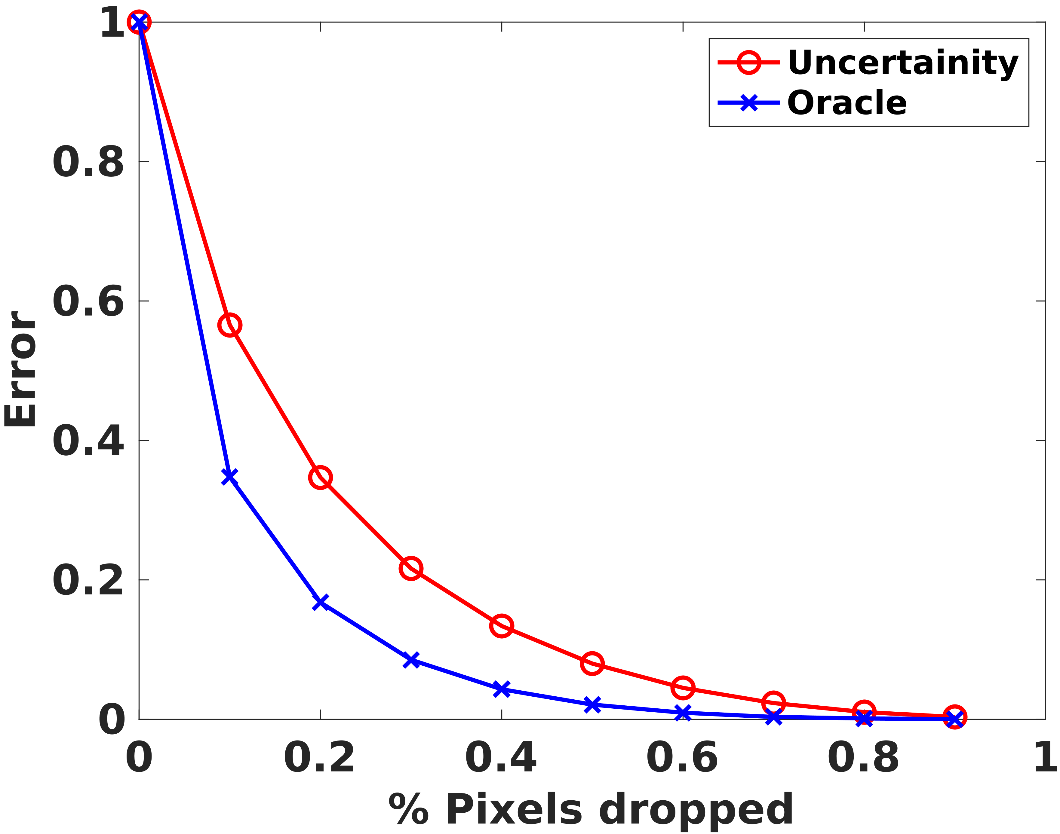
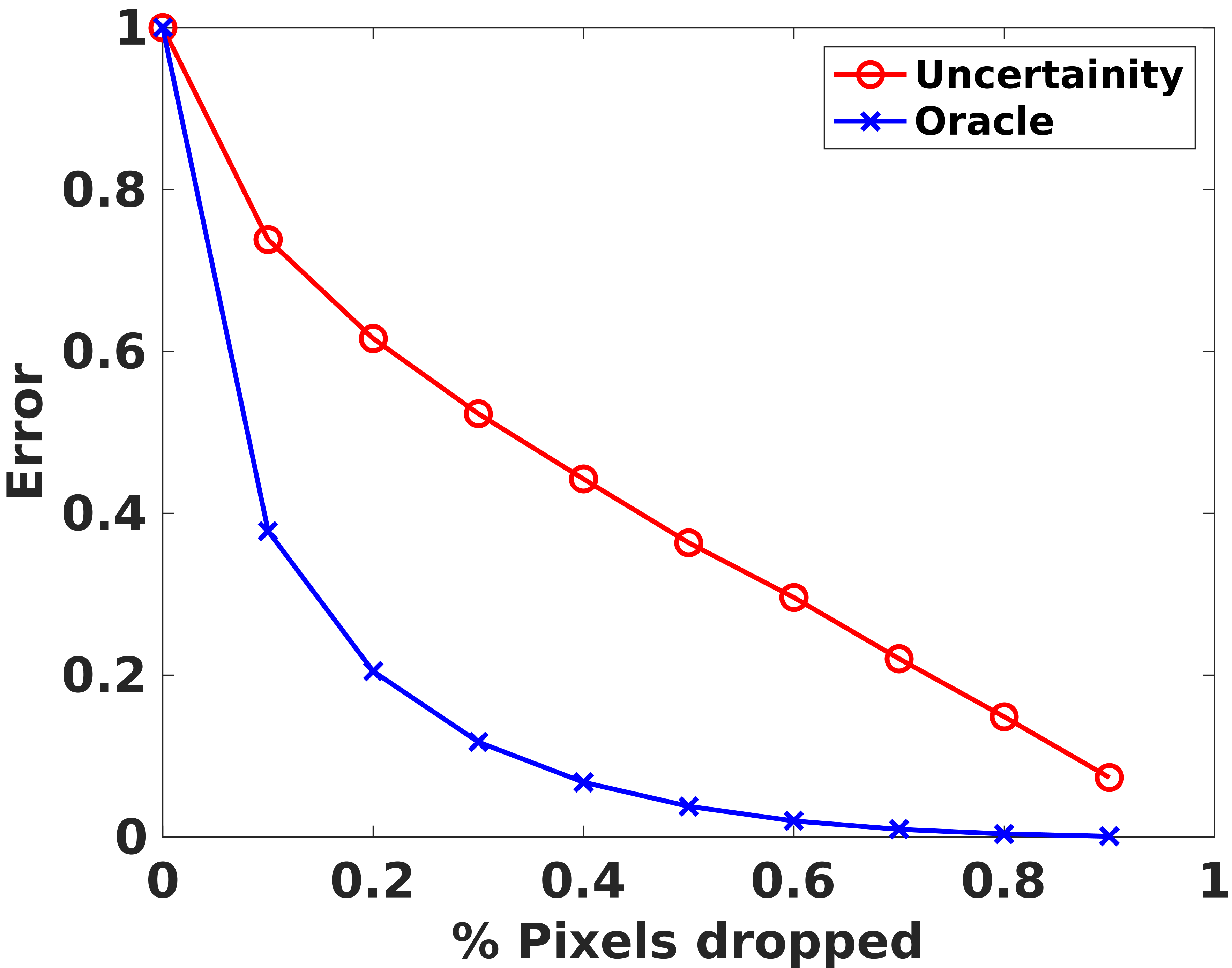
Sparsification plots provide a way to ascertain whether the uncertainty estimate is correlated with the prediction error [11]. Such plots are obtained by removing pixels with the highest uncertainty and measuring the error for the remaining pixels. If the predicted uncertainty is correlated with the error, the overall error should monotonically decrease as we remove more uncertainty pixels. We show the sparsification plots for the Aleatoric and Epistemic uncertainty estimates in Fig. 4. The optimal uncertainty estimate, would be perfectly correlated with the error, and the characteristic curve for the best possible uncertainty estimate can be obtained by dropping pixels with the highest errors first. We refer to this curve as Oracle in Fig. 4, and the closer the uncertainty sparsification curve to the Oracle curve, the better. The area between the sparsification curve and the oracle curve for the Aleatoric and Epistemic uncertainty estimations are 0.07 and 0.25, respectively. This shows that the prediction error has higher correlation with the aleatoric uncertainty estimation than the epistemic uncertainty estimation. Similar evaluation strategies have been used for evaluating the uncertainty estimates pertaining to optical flow estimation [11].

7.4 Crop-level Sample Selection

In the main paper, we pointed out that our sampling strategy can be used for picking out images from a large pool of unlabeled images, and it can also be used to pick out informative crops from an image. Depending on the annotation budget, it might be useful to get partial annotations for an image by picking out informative crops from an image and getting human annotations for the informative crops rather than annotating the entire image. The experiments on image level sample selection are discussed in the main paper. In Tab. 5, we present experiments pertaining to selecting informative crops from an image for human annotation. For the experiment, each image is divided into 16 non-overlapping crops and a single crop from each image is chosen for annotation. We compute the informativeness score for all 16 crops, and pick out the crop with the highest score. The informativeness score of crops are computed using the three sample selection strategies proposed in the main paper. We compare our proposed approach with two baselines: random crop selection and count based crop selection. For the random baseline, we pick out a crop at random from each image. For the count baseline, we pick out the crop with the highest count. Our proposed sample selection strategies outperforms the random selection and count selection baselines.

7.5 Image-level Sample Selection on Shanghaitech Part B

In the main paper, we presented image level sample selection experiments on Shanghaitech Part A [51] and NWPU [45] datasets. In Tab. 6, we present image level sample selection experiments on Shanghaitech Part B.

	Shtech Part B
Selection approach	#Train	MAE	RMSE
None (Pretrained)	NA	13.2	21.7
Random	50	9.4	16.6
Count	50	8.9	15.1
Aleatoric Uncertainty	50	8.7	14.3
Density based Ensemble Disagr.	50	8.5	13.6
KL-Ensemble Disagreement	50	8.8	15.4
Random	100	9.1	15.1
Count	100	8.0	13.5
Aleatoric Uncertainty	100	8.8	15.0
Density based Ensemble Disagreement	100	8.5	14.5
KL-Ensemble Disagreement	100	8.5	13.7
Full dataset (previous best method) [37]	400	7.6	11.8
Full dataset (CTN)	400	7.5	11.9

Table 6: Comparing different strategies for selecting images for annotation on Shanghaitech Part B dataset We train the network on the UCF-QNRF dataset, and use it to select images from the Shanghaitech Part B train data for acquiring annotation. We compare the random selection baseline with the proposed uncertainty-guided selection strategy. Our sample selection strategies outperform the two baselines when 50 images are sampled, and outperforms the random baseline when sampling 100 images.

References

- Babu et al. [2018] Deepak Babu, Neeraj Sajjan, VR Babu, and Mukundhan Srinivasan. Divide and grow: capturing huge diversity in crowd images with incrementally growing cnn. In Proceedings of the IEEE Conference on Computer Vision and Pattern Recognition, 2018.
- Babu Sam et al. [2017] Deepak Babu Sam, Shiv Surya, and R. Venkatesh Babu. Switching convolutional neural network for crowd counting. In Proceedings of the IEEE Conference on Computer Vision and Pattern Recognition, 2017.
- Cao et al. [2018] Xinkun Cao, Zhipeng Wang, Yanyun Zhao, and Fei Su. Scale aggregation network for accurate and efficient crowd counting. In Proceedings of the European Conference on Computer Vision, 2018.
- Chan and Vasconcelos [2009] Antoni B Chan and Nuno Vasconcelos. Bayesian poisson regression for crowd counting. In Proceedings of the International Conference on Computer Vision, 2009.
- Chen et al. [2012] Ke Chen, Chen Change Loy, Shaogang Gong, and Tony Xiang. Feature mining for localised crowd counting. In Proceedings of the British Machine Vision Conference, 2012.
- Cheng et al. [2019] Zhi-Qi Cheng, Jun-Xiu Li, Qi Dai, Xiao Wu, and Alexander G. Hauptmann. Learning spatial awareness to improve crowd counting. In Proceedings of the International Conference on Computer Vision, 2019.
- Gal and Ghahramani [2015] Yarin Gal and Zoubin Ghahramani. Bayesian convolutional neural networks with bernoulli approximate variational inference. arXiv preprint arXiv:1506.02158, 2015.
- Gao et al. [2019] Junyu Gao, Qi Wang, and Yuan Yuan. Scar: Spatial-/channel-wise attention regression networks for crowd counting. Neurocomputing, 363:1–8, 2019.
- Idrees et al. [2013] Haroon Idrees, Imran Saleemi, Cody Seibert, and Mubarak Shah. Multi-source multi-scale counting in extremely dense crowd images. In Proceedings of the IEEE Conference on Computer Vision and Pattern Recognition, 2013.
- Idrees et al. [2018] Haroon Idrees, Muhmmad Tayyab, Kishan Athrey, Dong Zhang, Somaya Al-Maadeed, Nasir Rajpoot, and Mubarak Shah. Composition loss for counting, density map estimation and localization in dense crowds. In Proceedings of the European Conference on Computer Vision, 2018.
- Ilg et al. [2018] Eddy Ilg, Ozgun Cicek, Silvio Galesso, Aaron Klein, Osama Makansi, Frank Hutter, and Thomas Brox. Uncertainty estimates and multi-hypotheses networks for optical flow. In Proceedings of the European Conference on Computer Vision, 2018.
- Jiang et al. [2019] Xiaolong Jiang, Zehao Xiao, Baochang Zhang, Xiantong Zhen, Xianbin Cao, David Doermann, and Ling Shao. Crowd counting and density estimation by trellis encoder-decoder networks. In Proceedings of the IEEE Conference on Computer Vision and Pattern Recognition, 2019.
- Kendall and Gal [2017] Alex Kendall and Yarin Gal. What uncertainties do we need in bayesian deep learning for computer vision? In Advances in Neural Information Processing Systems, 2017.
- Lempitsky and Zisserman [2010] Victor Lempitsky and Andrew Zisserman. Learning to count objects in images. In Advances in Neural Information Processing Systems, 2010.
- Lewis and Gale [1994] David D Lewis and William A Gale. A sequential algorithm for training text classifiers. In SIGIR’94, pages 3–12. Springer, 1994.
- Li et al. [2008] Min Li, Zhaoxiang Zhang, Kaiqi Huang, and Tieniu Tan. Estimating the number of people in crowded scenes by mid based foreground segmentation and head-shoulder detection. In Proceedings of the International Conference on Pattern Recognition, 2008.
- Li et al. [2018] Yuhong Li, Xiaofan Zhang, and Deming Chen. Csrnet: Dilated convolutional neural networks for understanding the highly congested scenes. In Proceedings of the IEEE Conference on Computer Vision and Pattern Recognition, 2018.
- Lian et al. [2019] Dongze Lian, Jing Li, Jia Zheng, Weixin Luo, and Shenghua Gao. Density map regression guided detection network for rgb-d crowd counting and localization. In Proceedings of the IEEE Conference on Computer Vision and Pattern Recognition, 2019.
- Lin et al. [2001] Sheng-Fuu Lin, Jaw-Yeh Chen, and Hung-Xin Chao. Estimation of number of people in crowded scenes using perspective transformation. IEEE Transactions on Systems, Man, and Cybernetics-Part A: Systems and Humans, 31(6):645–654, 2001.
- Liu et al. [2019a] Chenchen Liu, Xinyu Weng, and Yadong Mu. Recurrent attentive zooming for joint crowd counting and precise localization. In Proceedings of the IEEE Conference on Computer Vision and Pattern Recognition, 2019a.
- Liu et al. [2019b] Lingbo Liu, Zhilin Qiu, Guanbin Li, Shufan Liu, Wanli Ouyang, and Liang Lin. Crowd counting with deep structured scale integration network. In Proceedings of the International Conference on Computer Vision, 2019b.
- Liu et al. [2019c] Ning Liu, Yongchao Long, Changqing Zou, Qun Niu, Li Pan, and Hefeng Wu. Adcrowdnet: An attention-injective deformable convolutional network for crowd understanding. In Proceedings of the IEEE Conference on Computer Vision and Pattern Recognition, 2019c.
- Liu et al. [2019d] Weizhe Liu, Mathieu Salzmann, and Pascal Fua. Context-aware crowd counting. In Proceedings of the IEEE Conference on Computer Vision and Pattern Recognition, 2019d.
- Liu et al. [2019e] Yuting Liu, Miaojing Shi, Qijun Zhao, and Xiaofang Wang. Point in, box out: Beyond counting persons in crowds. In Proceedings of the IEEE Conference on Computer Vision and Pattern Recognition, 2019e.
- Lu et al. [2018] Erika Lu, Weidi Xie, and Andrew Zisserman. Class-agnostic counting. arXiv:1811.00472, 2018.
- Ma et al. [2019] Zhiheng Ma, Xing Wei, Xiaopeng Hong, and Yihong Gong. Bayesian loss for crowd count estimation with point supervision. In Proceedings of the International Conference on Computer Vision, 2019.
- Neal [2012] Radford M Neal. Bayesian learning for neural networks, volume 118. Springer Science & Business Media, 2012.
- Nix and Weigend [1994] David A Nix and Andreas S Weigend. Estimating the mean and variance of the target probability distribution. In Proceedings of IEEE International Conference on Neural Networks, 1994.
- Oh et al. [2019] Min-hwan Oh, Peder A Olsen, and Karthikeyan Natesan Ramamurthy. Crowd counting with decomposed uncertainty. arXiv preprint arXiv:1903.07427, 2019.
- Onoro-Rubio and López-Sastre [2016] Daniel Onoro-Rubio and Roberto J López-Sastre. Towards perspective-free object counting with deep learning. In Proceedings of the European Conference on Computer Vision, 2016.
- Ranjan et al. [2018] Viresh Ranjan, Hieu Le, and Minh Hoai. Iterative crowd counting. In Proceedings of the European Conference on Computer Vision, 2018.
- Ranjan et al. [2019] Viresh Ranjan, Mubarak Shah, and Minh Hoai. Crowd transformer network, 2019.
- Rumelhart et al. [1986] D. Rumelhart, G. Hinton, and R. Williams. Learning internal representations by error propagation. In Parallel Distributed Processing, volume 1, chapter 8, pages 318–362. MIT Press, Cambridge, MA, 1986.
- Sam et al. [2017] Deepak Babu Sam, Shiv Surya, and R Venkatesh Babu. Switching convolutional neural network for crowd counting. In Proceedings of the IEEE Conference on Computer Vision and Pattern Recognition, 2017.
- Settles [2009] Burr Settles. Active learning literature survey. Technical report, University of Wisconsin-Madison Department of Computer Sciences, 2009.
- Seung et al. [1992] H Sebastian Seung, Manfred Opper, and Haim Sompolinsky. Query by committee. In Proceedings of the fifth annual workshop on Computational learning theory, 1992.
- Shi et al. [2019] Miaojing Shi, Zhaohui Yang, Chao Xu, and Qijun Chen. Revisiting perspective information for efficient crowd counting. In Proceedings of the IEEE Conference on Computer Vision and Pattern Recognition, 2019.
- Simonyan and Zisserman [2014] Karen Simonyan and Andrew Zisserman. Very deep convolutional networks for large-scale image recognition. arXiv:1409.1556, 2014.
- Sindagi and Patel [2017a] Vishwanath A Sindagi and Vishal M Patel. Cnn-based cascaded multi-task learning of high-level prior and density estimation for crowd counting. In IEEE International Conference on Advanced Video and Signal Based Surveillance, 2017a.
- Sindagi and Patel [2017b] Vishwanath A Sindagi and Vishal M Patel. Generating high-quality crowd density maps using contextual pyramid cnns. In Proceedings of the International Conference on Computer Vision, 2017b.
- Srivastava et al. [2014] Nitish Srivastava, Geoffrey Hinton, Alex Krizhevsky, Ilya Sutskever, and Ruslan Salakhutdinov. Dropout: a simple way to prevent neural networks from overfitting. The journal of machine learning research, 15(1):1929–1958, 2014.
- Vaswani et al. [2017] Ashish Vaswani, Noam Shazeer, Niki Parmar, Jakob Uszkoreit, Llion Jones, Aidan N Gomez, Lukasz Kaiser, and Illia Polosukhin. Attention is all you need. In Advances in Neural Information Processing Systems, 2017.
- Wan et al. [2019] Jia Wan, Wenhan Luo, Baoyuan Wu, Antoni B. Chan, and Wei Liu. Residual regression with semantic prior for crowd counting. In Proceedings of the IEEE Conference on Computer Vision and Pattern Recognition, 2019.
- Wang et al. [2019] Qi Wang, Junyu Gao, Wei Lin, and Yuan Yuan. Learning from synthetic data for crowd counting in the wild. In Proceedings of the IEEE Conference on Computer Vision and Pattern Recognition, 2019.
- Wang et al. [2020] Qi Wang, Junyu Gao, Wei Lin, and Xuelong Li. Nwpu-crowd: A large-scale benchmark for crowd counting. arXiv preprint arXiv:2001.03360, 2020.
- Xu et al. [2019] Chenfeng Xu, Kai Qiu, Jianlong Fu, Song Bai, Yongchao Xu, and Xiang Bai. Learn to scale: Generating multipolar normalized density maps for crowd counting. In Proceedings of the International Conference on Computer Vision, 2019.
- Yan et al. [2019] Zhaoyi Yan, Yuchen Yuan, Wangmeng Zuo, Xiao Tan, Yezhen Wang, Shilei Wen, and Errui Ding. Perspective-guided convolution networks for crowd counting. In Proceedings of the International Conference on Computer Vision, 2019.
- Zhang et al. [2019] Anran Zhang, Lei Yue, Jiayi Shen, Fan Zhu, Xiantong Zhen, Xianbin Cao, and Ling Shao. Attentional neural fields for crowd counting. In Proceedings of the International Conference on Computer Vision, 2019.
- Zhang et al. [2015] Cong Zhang, Hongsheng Li, Xiaogang Wang, and Xiaokang Yang. Cross-scene crowd counting via deep convolutional neural networks. In Proceedings of the IEEE Conference on Computer Vision and Pattern Recognition, 2015.
- Zhang and Chan [2019] Qi Zhang and Antoni B. Chan. Wide-area crowd counting via ground-plane density maps and multi-view fusion cnns. In Proceedings of the IEEE Conference on Computer Vision and Pattern Recognition, 2019.
- Zhang et al. [2016] Yingying Zhang, Desen Zhou, Siqin Chen, Shenghua Gao, and Yi Ma. Single-image crowd counting via multi-column convolutional neural network. In Proceedings of the IEEE Conference on Computer Vision and Pattern Recognition, 2016.
- Zhao et al. [2019] Muming Zhao, Jian Zhang, Chongyang Zhang, and Wenjun Zhang. Leveraging heterogeneous auxiliary tasks to assist crowd counting. In Proceedings of the IEEE Conference on Computer Vision and Pattern Recognition, 2019.