Local Regression Distribution Estimators

Abstract

This paper investigates the large sample properties of local regression distribution estimators, which include a class of boundary adaptive density estimators as a prime example. First, we establish a pointwise Gaussian large sample distributional approximation in a unified way, allowing for both boundary and interior evaluation points simultaneously. Using this result, we study the asymptotic efficiency of the estimators, and show that a carefully crafted minimum distance implementation based on “redundant” regressors can lead to efficiency gains. Second, we establish uniform linearizations and strong approximations for the estimators, and employ these results to construct valid confidence bands. Third, we develop extensions to weighted distributions with estimated weights and to local $L^{2}$ least squares estimation. Finally, we illustrate our methods with two applications in program evaluation: counterfactual density testing, and IV specification and heterogeneity density analysis. Companion software packages in Stata and R are available.

Keywords: distribution and density estimation, local polynomial methods, uniform approximation, efficiency, optimal kernel, program evaluation.

1 Introduction

Kernel-based nonparametric estimation of distribution and density functions, as well as higher-order derivatives thereof, play an important role in econometrics. These nonparametric estimators often feature both as the main object of interest and as preliminary ingredients in multi-step semiparametric procedures (Newey and McFadden, 1994; Ichimura and Todd, 2007). Whitney Newey’s path-breaking contributions to non/semiparametric econometrics employing kernel smoothing are numerous. This paper hopes to honor his influential work in this area by studying the main large sample properties of a new class of local regression distribution estimators, which can be used for non/semiparametric estimation and inference.

The class of local regression distribution estimators is constructed using a local least squares approximation to the empirical distribution function of a random variable $x\in\mathcal{X}\subseteq\mathbb{R}$, where the localization at the evaluation point $\mathsf{x}\in\mathcal{X}$ is implemented via a kernel function and a bandwidth parameter. The local functional form approximation is done using a finite-dimension basis function. When the basis function contains polynomials up to order $p\in\mathbb{N}$, the associated least squares coefficients give estimators of the distribution function, density function, and higher-order derivatives (up to order $p-1$), all evaluated at $\mathsf{x}\in\mathcal{X}$. If only a polynomial basis is used, then the estimator reduces to the one recently proposed in Cattaneo, Jansson, and Ma (2020).

We present two main large sample distributional results for the local regression distribution estimators. First, in Section 3, we establish a pointwise (in $\mathsf{x}\in\mathcal{X}$) Gaussian distributional approximation with consistent standard errors. Because these estimators have a U-statistic structure with an $n$-varying kernel, where $n$ denotes the sample size, we construct a fully automatic Studentization given a choice of basis, kernel, and bandwidth. Furthermore, we show that when the basis function includes polynomials, the associated density and its higher-order derivatives estimators are boundary adaptive without further modifications. This result generalizes Cattaneo, Jansson, and Ma (2020) by allowing for arbitrary local basis functions, which is particularly useful for efficiency considerations.

To be more precise, for the special case of local polynomial density estimation, Cattaneo, Jansson, and Ma (2020) showed that the asymptotic variance of the estimator is of the “sandwich” form, which does not reduce to a single matrix (up to a proportional factor) by a choice of kernel function. This finding indicates that more efficient estimators can be constructed via a minimum distance approach based on “redundant” regressors, following well-known results in econometrics (Newey and McFadden, 1994). In Section 3.3, we present a novel minimum distance construction for estimation of the density and its derivatives, and obtain an efficiency bound for the new minimum distance density estimator. Furthermore, we show that the efficiency bound coincides with the well-known asymptotic variance lower bound for kernel-based density estimation (Granovsky and Müller, 1991; Cheng, Fan, and Marron, 1997). We also show that this efficiency bound is tight: we construct a feasible minimum distance procedure exploiting carefully chosen redundant regressors, which leads to an estimator with asymptotic variance arbitrarily close to the theoretical efficiency bound. These results offer not only a novel theoretical perspective on efficiency of classical nonparametric kernel-based density estimation, but also a new class of more efficient boundary adaptive density estimators for practice. We also discuss how these results generalize to other local regression distribution estimators in the supplemental appendix.

Our second main large sample distributional result, in Section 4, concerns uniform estimation and inference over a region $\mathcal{I}\subseteq\mathcal{X}$, based on either the basic local regression distribution estimators or the associated more efficient estimators obtained via our proposed minimum distance procedure. More precisely, we establish a strong approximation to the boundary adaptive Studentized statistic, uniformly over $\mathsf{x}\in\mathcal{I}$, relying on a “coupling” result in Giné, Koltchinskii, and Sakhanenko (2004); see also Rio (1994) and Giné and Nickl (2010) for closely related results, and Zaitsev (2013) for a review on strong approximation methods. This approach allows us to deduce a distributional approximation for many functionals of the Studentized statistic, including its supremum, following ideas in Chernozhukov, Chetverikov, and Kato (2014b). For further discussion and references on strong approximations and their applications to non/semiparametric econometrics see Chernozhukov, Chetverikov, and Kato (2014a), Belloni, Chernozhukov, Chetverikov, and Kato (2015), Belloni, Chernozhukov, Chetverikov, and Fernandez-Val (2019), and Cattaneo, Farrell, and Feng (2020), Cattaneo, Crump, Farrell, and Feng (2021), and references therein.

We employ our strong approximation results for local regression distribution estimators to construct asymptotically valid confidence bands for the density function and derivatives thereof. Other applications of our results, not discussed here to conserve space, include specification and shape restriction testing. As a by-product, we also establish a linear approximation to the boundary adaptive Studentized statistic, uniformly over $\mathsf{x}\in\mathcal{I}$, which gives uniform convergence rates and can be used for further theoretical developments. See the supplemental appendix for more details.

In addition to our main large sample results for local regression distribution and related estimators, we briefly discuss several extensions in Section 5. First, we allow for a weighted empirical distribution function entering our estimators, where the weights themselves may be estimated. Our results continue to hold in this more general case, which is practically relevant as illustrated in our empirical applications. Second, we present and study an alternative class of estimators that employ a non-random $L^{2}$ loss function, instead of the more standard least squares approximation underlying our local regression distribution estimators. These alternative estimators enjoy certain theoretical advantages, but require ex-ante knowledge of the boundary location of $\mathcal{X}$. In particular, we show in the supplemental appendix how these alternative estimators can be implemented to achieve maximum asymptotic efficiency in estimating the density function and its derivatives. Third, we also discuss incorporating shape restrictions using the general local basis function entering the local regression distribution estimators.

Finally, in Section 6, we illustrate our methods with two applications in program evaluation (for a review see Abadie and Cattaneo, 2018). First, we discuss counterfactual density analysis following DiNardo, Fortin, and Lemieux (1996); see also Chernozhukov, Fernandez-Val, and Melly (2013) for related discussion based on distribution functions. Second, we discuss specification testing and heterogeneity analysis in the context of instrumental variables following Kitagawa (2015) and Abadie (2003), respectively; see also Imbens and Rubin (2015) for background and other applications of nonparametric density estimation to causal inference and program evaluation. In all these applications, we develop formal estimation and inference methods based on nonparametric density estimation using local regression distribution estimators implemented with weighted distribution functions. We showcase our new methods using a subsample of the data in Abadie, Angrist, and Imbens (2002), corresponding to the Job Training Partnership Act (JTPA).

From both methodological and technical perspectives, our proposed class of local regression distribution estimators is different from, and exhibits demonstrable advantages over, other related estimators available in the literature. For the special case of density estimation (i.e., when the basis function is taken to be polynomial), our resulting kernel-based density estimator enjoys boundary carpentry over the possibly unknown boundary of $\mathcal{X}$, does not require preliminary smoothing of the data and hence avoids preliminary tuning parameter choices, and is easy to implement and interpret. Cattaneo, Jansson, and Ma (2020) gave a detailed discussion of that density estimator and related approaches in the literature, which include the influential local polynomial estimator of Cheng, Fan, and Marron (1997) and related estimators (Zhang and Karunamuni, 1998; Karunamuni and Zhang, 2008, and referneces therein). The class of estimators we consider here can be more efficient by employing minimum distance estimation ideas (Section 3), easily delivers intuitive estimators of density-weighted averages (Section 5.1), and allows for incorporating shape and other restrictions (Section 5.3), among other features that we discuss below. Last but not least, some of the technical results presented herein for the general class of estimators, such as asymptotic efficiency (Section 3.3) and uniform inference (Section 4) are new, even for the special case of density estimation in Cattaneo, Jansson, and Ma (2020).

The rest of the paper proceeds as follows. Section 2 introduces the class of local regression distribution estimators. Section 3 establishes a pointwise distributional approximation, along with a consistent standard error estimator, and discusses efficiency focusing in particular on the leading special case of density estimation. Section 4 establishes uniform results, including valid linearizations and strong approximations, which are then used to construct confidence bands. Section 5 discusses extensions of our methodology, while Section 6 illustrates our new methods with two distinct program evaluation applications. Section 7 concludes. The supplemental appendix (SA) includes all proofs of our theoretical results as well as other technical, methodological and numerical results that may be of independent interest. Software packages for Stata and R implementing the main results in this paper are discussed in Cattaneo, Jansson, and Ma (2021).

2 Setup

Suppose $x_{1},x_{2},\dots,x_{n}$ is a random sample from a univariate random variable $x$ with absolute continuous cumulative distribution function $F(\cdot)$, and associated Lebesgue density $f(\cdot)$, over its support $\mathcal{X}\subseteq\mathbb{R}$, which may be compact and not necessarily known. We propose, and study the large sample properties of a new class of nonparametric estimators of $F(\cdot)$, $f(\cdot)$, and derivatives thereof, both pointwise at $\mathsf{x}\in\mathcal{X}$ and uniformly over some region $\mathcal{I}\subseteq\mathcal{X}$.

Our proposed estimators are applicable whenever $F(\cdot)$ is suitably smooth near $\mathsf{x}$ and admits a sufficiently accurate linear-in-parameters local approximation of the form:

$$\varrho(h,\mathsf{x})=\sup_{|x-\mathsf{x}|\leq h}\Big{|}F(x)-R(x-\mathsf{x})^{\prime}\theta(\mathsf{x})\Big{|}\qquad\text{is small for $h$ small},$$ (1)

where $R(\cdot)$ is a known local basis function and $\theta(\mathsf{x})$ is a parameter vector to be estimated. As an estimator of $\theta(\mathsf{x})$ in (1), we consider the local regression estimator

$$\hat{\theta}(\mathsf{x})=\operatorname*{argmin}_{\theta}\sum_{i=1}^{n}W_{i}\left(\hat{F}_{i}-R_{i}^{\prime}\theta\right)^{2},$$ (2)

where $W_{i}=K((x_{i}-\mathsf{x})/h)/h$ for some kernel $K(\cdot)$ and some bandwidth $h,$ $R_{i}=R(x_{i}-\mathsf{x})$, and

$$\hat{F}_{i}=\frac{1}{n}\sum_{j=1}^{n}\mathds{1}(x_{j}\leq x_{i})$$ (3)

is the empirical distribution function evaluated at $x_{i}$, with $\mathds{1}(\cdot)$ denoting the indicator function.

The generic formulation (1) is motivated in part by the important special case where $F(\cdot)$ is sufficiently smooth, in which case

$$F(x)\approx F(\mathsf{x})+f(\mathsf{x})(x-\mathsf{x})+...+f^{(p-1)}(\mathsf{x})\frac{1}{p!}(x-\mathsf{x})^{p}\qquad\text{for }x\approx\mathsf{x},$$ (4)

and $f^{(s)}(\mathsf{x})=\left.\mathrm{d}^{s}f(x)/\mathrm{d}x^{s}\right|_{x=\mathsf{x}}$ are higher-order density derivatives. Of course, the approximation (4) is of the form (1) with $R(u)=(1,u,\cdots,u^{p}/p!)^{\prime}$, and hence $\theta(\mathsf{x})=(F(\mathsf{x}),f(\mathsf{x}),\cdots,f^{(p-1)}(\mathsf{x}))^{\prime}$. In such special case, the estimator $\hat{\theta}(\mathsf{x})$ corresponds to one of the estimators introduced in Cattaneo, Jansson, and Ma (2020). But, as further discussed below, other choices of $R(\cdot)$ and/or $\theta(\mathsf{\cdot})$ can be attractive, and as a consequence we take (1) as the starting point for our analysis. Section 5 discusses other extensions and generalization of the basic local regression distribution estimator $\hat{\theta}(\mathsf{x})$ in (2).

The class of estimators defined in (2) is motivated by standard local polynomial regression methods (Fan and Gijbels, 1996). However, well-known results for local polynomial regression are not applicable to the local regression distribution estimator, $\hat{\theta}(\mathsf{x})$, because the empirical distribution function estimator, $\hat{F}_{i}$, which plays the role of the “dependent” variable in the construction, depends on not only $x_{i}$ but also all of the “independent” observations $x_{1},x_{2},\dots,x_{n}$. This implies that, unlike the case of standard local polynomial regression, $\hat{\theta}(\mathsf{x})$ cannot be studied by conditioning on the “covariates” $x_{1},x_{2},\dots,x_{n}$. Instead, we employ U-statistic methods for analyzing the statistical properties of $\hat{\theta}(\mathsf{x})$. This observation explains the quite different asymptotic variance of our estimator: see Section 3.3 for details. Furthermore, as discussed in Section 5.1, when a weighted distribution function is used in place of $\hat{F}_{i}$ in (2), the resulting (weighted) local regression distribution estimators are consistent for a density-weighted regression function, as opposed to being consistent for the regression function itself (as it is the case for standard local polynomial regression methods). Finally, the SA highlights other technical differences between the two types of local regression estimators.

3 Pointwise Distribution Theory

This section discusses the large sample properties of the estimator $\hat{\theta}(\mathsf{x}),$ pointwise in $\mathsf{x}\in\mathcal{X}$. We first establish asymptotic normality, and then discuss asymptotic efficiency. Other results are reported in the SA to conserve space. We drop the dependence on the evaluation point $\mathsf{x}$ whenever possible.

3.1 Assumptions

We impose the following assumption throughout this section. We do not restrict the support of $\mathcal{X}$, which can be a compact set or unbounded, because our estimator automatically adapts to boundary evaluation points.

Assumption 1

$x_{1},\dots,x_{n}$ is a random sample from a distribution $F(\cdot)$ supported on $\mathcal{X}\subseteq\mathbb{R}$, and $\mathsf{x}\in\mathcal{X}$.

(i) For some $\delta>0,$ $F(\cdot)$ is absolutely continuous on $[\mathsf{x}-\delta,\mathsf{x}+\delta]$ with a density $f(\cdot)$ admitting constants $f(\mathsf{x}-)$, $\dot{f}(\mathsf{x}-)$, $f(\mathsf{x}+)$, and $\dot{f}(\mathsf{x}+)$ such that

$$\sup_{u\in[-\delta,0)}\frac{|f(\mathsf{x}+u)-f(\mathsf{x}-)-\dot{f}(\mathsf{x}-)u|}{|u|^{2}}+\sup_{u\in(0,\delta]}\frac{|f(\mathsf{x}+u)-f(\mathsf{x}+)-\dot{f}(\mathsf{x}+)u|}{|u|^{2}}<\infty.$$

(ii) $K(\cdot)$ is nonnegative, symmetric, and continuous on its support $[-1,1]$, and integrates to 1.

(iii) $R(\cdot)$ is locally bounded, and there exists a positive-definite diagonal matrix $\Upsilon_{h}$ for each $h>0$, such that $\Upsilon_{h}R(u)=R(u/h)$.

(iv) Let $\mathcal{X}_{h,\mathsf{x}}=\frac{\mathcal{X}-\mathsf{x}}{h}$. For all $h$ sufficiently small, the minimum eigenvalues of $\Gamma_{h,\mathsf{x}}$ and $h^{-1}\Sigma_{h,\mathsf{x}}$ are bounded away from zero, where

$$\Gamma_{h,\mathsf{x}} =\int\nolimits_{\mathcal{X}_{h,\mathsf{x}}}R(u)R(u)^{\prime}K(u)f(\mathsf{x}+hu)\mathrm{d}u,$$

$$\Sigma_{h,\mathsf{x}} =\int_{\mathcal{X}_{h,\mathsf{x}}}\int_{\mathcal{X}_{h,\mathsf{x}}}R(u)R(v)^{\prime}\Big{[}F(\mathsf{x}+h\min\{u,v\})-F(\mathsf{x}+hu)F(\mathsf{x}+hv)\Big{]}$$

$$\qquad\qquad\qquad\qquad\cdot K(u)K(v)f(\mathsf{x}+hu)f(\mathsf{x}+hv)\mathrm{d}u\mathrm{d}v.$$

Part (i) imposes smoothness conditions on the distribution function $F(\cdot)$, separately for the two regions on the left and on the right of the evaluation point $\mathsf{x}$. In most applications, the distribution function will also be smooth at the evaluation point, in which case $f(\mathsf{x}-)=f(\mathsf{x}+)$ and $\dot{f}(\mathsf{x}-)=\dot{f}(\mathsf{x}+)$. However, there are important situations where $F(\cdot)$ only has one-sided derivatives, such as at boundary or kink evaluation points. Part (ii) imposes standard restrictions on the kernel function, which allows for all commonly used (compactly supported) second-order kernel functions. Part (iii) requires that the local basis $R(\cdot)$ can be stabilized by a suitable normalization. Parts (iv) give assumptions on two (non-random) matrices which will feature in the asymptotic distribution.

The error of the approximation in (1) depends on the choice of $R(\cdot)$ and $\theta$, and is quantified by $\varrho(h)$, where we suppress the dependence on the evaluation point $\mathsf{x}$ to save notation. The approximation error will be required to be “small” in the sense that $n\varrho(h)^{2}/h\to 0$. In the cases of main interest (i.e., when $R(\cdot)$ is polynomial), we have either $\varrho(h)=O(h^{p+1})$ or $\varrho(h)=o(h^{p})$ for some $p$. The condition can therefore be stated as $nh^{2p+1}\to 0$ and $nh^{2p-1}=O(1)$, respectively, in those cases.

We do not discuss how to choose the bandwidth $h$, or the order $p$ if $R(\cdot)$ contains polynomials, as both choices can be developed following standard ideas in the local polynomial literature. We focus instead on distributional approximation (Section 3.2) and asymptotic variance minimization (Section 3.3), given a choice of bandwidth sequence and polynomial order. Bandwidth selection can be developed by extending the results in Cattaneo, Jansson, and Ma (2020) and polynomial order selection can be developed following Fan and Gijbels (1996, Section 3.3). In particular, a larger $p$ can lead to more bias reduction whenever the target population function is smooth enough at the expense of a larger asymptotic variance. We discuss this trade-off explicitly in our efficiency calculations (Section 3.3).

3.2 Asymptotic Normality

We show that, under regularity conditions and if $h$ vanishes at a suitable rate as $n\to\infty$, then

$$\hat{\Omega}^{-1/2}(\hat{\theta}-\theta)\rightsquigarrow\mathcal{N}(0,I),\qquad\hat{\Omega}=\hat{\Gamma}^{-1}\hat{\Sigma}\hat{\Gamma}^{-1},$$ (5)

where

$$\hat{\Gamma}=\frac{1}{n}\sum_{i=1}^{n}W_{i}R_{i}R_{i}^{\prime},\qquad\hat{\Sigma}=\frac{1}{n^{2}}\sum_{i=1}^{n}\hat{\psi}_{i}\hat{\psi}_{i}^{\prime},\qquad\hat{\psi}_{i}=\frac{1}{n}\sum_{j=1}^{n}W_{j}R_{j}(\mathds{1}(x_{i}\leq x_{j})-\hat{F}_{j}).$$

It follows from this result that inference on $\theta$ can be based on $\hat{\theta}$ by employing the (pointwise) distributional approximation $\hat{\theta}\overset{a}{\sim}\mathcal{N}(\theta,\hat{\Omega})$. The three matrices, $\hat{\Gamma}$, $\hat{\Sigma}$ and $\hat{\Omega}$, depend on the evaluation point $\mathsf{x}$, but such dependence is again suppressed for simplicity. This distributional result will rely on the “small” bias condition $n\varrho(h)^{2}/h\to 0$ mentioned above, which makes the asymptotic approximation (or smoothing) bias of $\hat{\theta}$ negligible relative to the standard error. From an inference perspective, such bias condition can be achieved by employing undersmoothing or robust bias correction: see Calonico, Cattaneo, and Farrell (2018, 2020) for discussion and background references. The SA includes more details on the bias of the estimator.

To provide some insight into the distributional approximation (5), and to see why it cannot be established using standard results for local polynomial regression, first observe that

$$\hat{\theta}-\theta=\hat{\Gamma}^{-1}S,\qquad S=\frac{1}{n}\sum_{i=1}^{n}W_{i}R_{i}(\hat{F}_{i}-R_{i}^{\prime}\theta),$$

assuming $\hat{\Gamma}$ is invertible with probability approaching one. The statistic $S$ can be written as

$$S=U+B,\qquad U=\frac{1}{n(n-1)}\sum_{i,j=1,i\neq j}^{n}W_{j}R_{j}\Big{(}\mathds{1}(x_{i}\leq x_{j})-F(x_{j})\Big{)},$$ (6)

where $B$ consists of a leave-in bias term and a smoothing bias term. Since $S$ is approximately a second-order $U$-statistic, result (5) should follow from a central limit theorem for ($n$-varying) $U$-statistics under suitable regularity conditions, including conditions ensuring that the approximation errors are negligible. More specifically, result (5) follows if $U$ is asymptotically mean-zero Gaussian $\mathbb{V}[U]^{-1/2}U\rightsquigarrow\mathcal{N}(0,I)$, where $\mathbb{V}[U]$ denotes the variance of $U$, $\mathbb{V}[U]^{-1/2}B\to_{\mathbb{P}}0$, and if the variance estimator $\hat{\Sigma}$ is consistent in the sense that $\mathbb{V}[U]^{-1}(\hat{\Sigma}-\mathbb{V}[U])\to_{\mathbb{P}}0$. Moreover, the projection theorem for $U$-statistics implies that, under appropriate regularity conditions,

$$\mathbb{V}[U]\approx\frac{1}{n}\mathbb{E}[\psi_{i}\psi_{i}^{\prime}],\qquad\psi_{i}=\mathbb{E}[W_{j}R_{j}\mathds{1}(x_{i}\leq x_{j})-F(x_{j})|x_{i}],$$

which motivates the functional form of the variance estimator $\hat{\Sigma}$ used to form $\hat{\Omega}$.

The following theorem formalizes the above intuition with precise sufficient conditions.

Theorem 1 (Pointwise Asymptotic Normality)

Suppose Assumption 1 holds. If $n\varrho(h)^{2}/h\to 0$ and $nh^{2}\to\infty$, then (5) holds.

This theorem establishes a (pointwise) Gaussian distributional approximation for the Studentized statistic $\hat{\Omega}^{-1/2}(\hat{\theta}-\theta)$, which is valid for each evaluation point $\mathsf{x}\in\mathcal{X}$. For example, letting $c$ be a vector of conformable dimension and $\alpha\in(0,1)$, this result justifies the standard $100(1-\alpha)\%$ confidence interval

$$\text{CI}_{\alpha}(\mathsf{x})=\left[c^{\prime}\hat{\theta}(\mathsf{x})-\mathfrak{q}_{1-\alpha/2}\sqrt{c^{\prime}\hat{\Omega}(\mathsf{x})c}~{},~{}c^{\prime}\hat{\theta}(\mathsf{x})-\mathfrak{q}_{\alpha/2}\sqrt{c^{\prime}\hat{\Omega}(\mathsf{x})c}\right],$$

where $\mathfrak{q}_{a}=\inf\{u\in\mathbb{R}:\mathbb{P}\left[\mathcal{N}(0,1)\leq u\right]\geq a\}$. The above confidence interval is asymptotically valid for each evaluation point $\mathsf{x}$, which is reflected by the notation $\text{CI}_{\alpha}(\mathsf{x})$. That is,

$$\lim_{n\to\infty}\mathbb{P}\Big{[}c^{\prime}\theta(\mathsf{x})\in\text{CI}_{\alpha}(\mathsf{x})\Big{]}=1-\alpha,\qquad\text{for all }\mathsf{x}\in\mathcal{X}.$$

Section 4 develops asymptotically valid confidence bands, which will be denoted by $\text{CI}_{\alpha}(\mathcal{I})$ for some region $\mathcal{I}\subseteq\mathcal{X}$.

3.3 Efficiency

As it is well known in the literature (Fan and Gijbels, 1996), the standard local polynomial regression estimator of $\mathbb{E}[y|x=\mathsf{x}]$, for dependent variable $y$ and independent variable $x$, has a limiting asymptotic variance of the “sandwich form” $e_{0}^{\prime}\Gamma^{-1}A\Gamma^{-1}e_{0}$, where $e_{\ell}$ denotes the $(\ell+1)$th standard basis vector, and

$$\Gamma=f(\mathsf{x})\int_{-1}^{1}R(u)R(u)^{\prime}K(u)\mathrm{d}u,\quad A=\mathbb{V}[y|x=\mathsf{x}]f(\mathsf{x})\int_{-1}^{1}R(u)R(u)^{\prime}K(u)^{2}\mathrm{d}u.$$

This variance structure implies that setting $K(\cdot)$ to be the uniform kernel makes $\Gamma$ proportional to $A$ (i.e., $K(u)=K(u)^{2}$ whenever $K(u)=\mathds{1}(|u|\leq 1)$), and hence minimizes the above asymptotic variance, at least in the sense that $\Gamma^{-1}A\Gamma^{-1}\geq A^{-1}$. See also Granovsky and Müller (1991) for a more general discussion on the optimality of the uniform kernel for kernel-based estimation.

Unlike the case of the asymptotic variance of local polynomial regression, however, our local regression distribution estimators exhibit a more complex and uneven asymptotic variance formula due to their construction. As a result, employing the uniform kernel may not exhaust the potential efficiency gains. For example, in the case of local polynomial density estimation (Cattaneo, Jansson, and Ma, 2020), $R(u)$ is polynomial of order $p\geq 1$ and the asymptotic variance of the density estimator $\hat{f}(\mathsf{x})=e_{1}^{\prime}\hat{\theta}(\mathsf{x})$ takes the form $e_{1}^{\prime}\Gamma^{-1}\Sigma\Gamma^{-1}e_{1}$ with

$$\Sigma=f(\mathsf{x})^{3}\int_{-1}^{1}\int_{-1}^{1}\min\{u,v\}R(u)R(v)^{\prime}K(u)K(v)\mathrm{d}u\mathrm{d}v,$$

which implies that $\Gamma$ is no longer proportional to $\Sigma$ even when the kernel function is uniform. (To show this result, one first recognizes that the asymptotic variance of $\hat{f}(\mathsf{x})$ is $h^{-1}e_{1}^{\prime}\Gamma^{-1}_{h}\Sigma_{h}\Gamma^{-1}_{h}e_{1}$, where the matrices are defined in Assumption 1. Then the expression reduces to $e_{1}^{\prime}\Gamma^{-1}\Sigma\Gamma^{-1}e_{1}$ after taking the limit $h\to 0$, provided that $\mathsf{x}$ is an interior evaluation point. See the SA for omitted details.) This observation applies to the general case where the local basis function $R(\cdot)$ needs not to be of polynomial form, or when higher-order derivatives are of interest. See the SA for further discussion and detailed formulas.

In this section we employ a minimum distance approach to develop a lower bound on the asymptotic variance of the local regression distribution estimators, and also propose more efficient estimators based on the observation that their asymptotic variance is of the sandwich form $\Gamma^{-1}\Sigma\Gamma^{-1}$ but with $\Gamma$ not proportional to $\Sigma$ even when the uniform kernel is used.

To motivate our approach, notice that in many cases it is possible to specify $R(\cdot)$ in such a way that $\theta$ can be partitioned as $\theta=(\theta_{1}^{\prime},\theta_{2}^{\prime})^{\prime},$ where $\theta_{2}=0$. In such cases several distinct estimators of $\theta_{1}$ are available. To describe some leading candidates and their salient properties, partition $\hat{\theta}$, $\hat{\Gamma}$, $\hat{\Sigma}$, and $\hat{\Omega}$ conformable with $\theta$ as $\hat{\theta}=(\hat{\theta}_{1}^{\prime},\hat{\theta}_{2}^{\prime})^{\prime}$ and

$$\hat{\Gamma}=\left(\begin{array}[c]{cc}\hat{\Gamma}_{11}&\hat{\Gamma}_{12}\\ \hat{\Gamma}_{21}&\hat{\Gamma}_{22}\end{array}\right),\qquad\hat{\Sigma}=\left(\begin{array}[c]{cc}\hat{\Sigma}_{11}&\hat{\Sigma}_{12}\\ \hat{\Sigma}_{21}&\hat{\Sigma}_{22}\end{array}\right),\qquad\hat{\Omega}=\left(\begin{array}[c]{cc}\hat{\Omega}_{11}&\hat{\Omega}_{12}\\ \hat{\Omega}_{21}&\hat{\Omega}_{22}\end{array}\right).$$

The “short” regression counterpart of $\hat{\theta}_{1}$ obtained by dropping $R_{2}(\cdot)$ from $R(\cdot)=(R_{1}(\cdot)^{\prime},R_{2}(\cdot)^{\prime})^{\prime}$ is given by

$$\hat{\theta}_{\mathtt{R},1}=\hat{\theta}_{1}+\hat{\Gamma}_{11}^{-1}\hat{\Gamma}_{12}\hat{\theta}_{2},$$

while an optimal minimum distance estimator of $\theta_{1}$ is given by

$$\hat{\theta}_{\mathtt{MD},1}=\operatorname*{argmin}_{\theta_{1}}\binom{\hat{\theta}_{1}-\theta_{1}}{\hat{\theta}_{2}}^{\prime}\hat{\Omega}^{-1}\binom{\hat{\theta}_{1}-\theta_{1}}{\hat{\theta}_{2}}=\hat{\theta}_{1}-\hat{\Omega}_{12}\hat{\Omega}_{22}^{-1}\hat{\theta}_{2}.$$ (7)

As a by-product of results obtained when establishing (5), it follows that

$$\hat{\Omega}_{11}^{-1/2}(\hat{\theta}_{1}-\theta_{1}) \rightsquigarrow\mathcal{N}(0,I),$$

$$\hat{\Omega}_{\mathtt{R},11}^{-1/2}(\hat{\theta}_{\mathtt{R},1}-\theta_{1}) \rightsquigarrow\mathcal{N}(0,I),\qquad\hat{\Omega}_{\mathtt{R},11}=\hat{\Gamma}_{11}^{-1}\hat{\Sigma}_{11}\hat{\Gamma}_{11}^{-1},$$

$$\text{and}\qquad\hat{\Omega}_{\mathtt{MD},11}^{-1/2}(\hat{\theta}_{\mathtt{MD},1}-\theta_{1}) \rightsquigarrow\mathcal{N}(0,I),\qquad\hat{\Omega}_{\mathtt{MD},11}=\hat{\Omega}_{11}-\hat{\Omega}_{12}\hat{\Omega}_{22}^{-1}\hat{\Omega}_{21},$$

under regularity conditions. Since $\hat{\Omega}$ is of “sandwich” form, the estimators $\hat{\theta}_{1}$ and $\hat{\theta}_{\mathtt{R},1}$ cannot be ranked in terms of (asymptotic) efficiency in general. On the other hand, $\hat{\theta}_{\mathtt{MD},1}$ will always be (weakly) superior to both $\hat{\theta}_{1}$ and $\hat{\theta}_{\mathtt{R},1}$. In fact, because

$$\hat{\theta}_{1}=\operatorname*{argmin}_{\theta_{1}}\binom{\hat{\theta}_{1}-\theta_{1}}{\hat{\theta}_{2}}^{\prime}\left(\begin{array}[c]{cc}\hat{\Omega}_{11}^{-1}&0\\ 0&\hat{\Omega}_{22}^{-1}\end{array}\right)\binom{\hat{\theta}_{1}-\theta_{1}}{\hat{\theta}_{2}},$$

and

$$\hat{\theta}_{\mathtt{R},1}=\operatorname*{argmin}_{\theta_{1}}\binom{\hat{\theta}_{1}-\theta_{1}}{\hat{\theta}_{2}}^{\prime}\hat{\Gamma}\binom{\hat{\theta}_{1}-\theta_{1}}{\hat{\theta}_{2}},$$

each estimator admits a minimum distance interpretation, but only $\hat{\theta}_{\mathtt{MD},1}$ can be interpreted as an optimal minimum distance estimator based on $\hat{\theta}$. See Newey and McFadden (1994) for more discussion on minimum distance estimation.

As a consequence, we investigate whether an appropriately implemented $\hat{\theta}_{\mathtt{MD},1}$ can lead to asymptotic efficiency gains relative to $\hat{\theta}_{1}$ and $\hat{\theta}_{\mathtt{R},1}$. More generally, as a by-product, we obtain an efficiency bound among minimum distance estimators and show that this bound coincides with those known in the literature for kernel-based density estimation at interior points (Granovsky and Müller, 1991; Cheng, Fan, and Marron, 1997).

In the remaining of this section we focus on the case of local polynomial density estimation at an interior point for concreteness, but the SA presents more general results. Consequently, we assume that $F(\cdot)$ is $p$-times continuously differentiable in a neighborhood of $\mathsf{x}$. Then, (4) is satisfied and a natural choice of $R(\cdot)$ is

$$R(u)=\Big{(}R_{1}(u)^{\prime},R_{2}(u)^{\prime}\Big{)}^{\prime}=\Big{(}1,P(u)^{\prime},Q(u)^{\prime}\Big{)}^{\prime},$$ (8)

where $P(u)=(u,u^{2}/2,\cdots,u^{p}/p!)^{\prime}$ is a polynomial basis, and $Q(\cdot)$ represent redundant regressors. Therefore, in our minimum distance construction, the parameters are

$$\theta=\Big{(}\underbrace{F(\mathsf{x})}_{\text{intercept}},\ \underbrace{f(\mathsf{x}),\ \cdots,\ f^{(p-1)}(\mathsf{x})}_{\text{slope, }P(\cdot)},\ \underbrace{0,\ \cdots,\ 0}_{\text{redundant, }Q(\cdot)}\Big{)}^{\prime},$$ (9)

with smoothing error of order $\varrho(h)=o(h^{p})$.

With (8) and (9), we define the minimum distance density estimator as $\hat{f}_{\mathtt{MD}}(\mathsf{x})=e_{1}^{\prime}\hat{\theta}_{\mathtt{MD,1}}$. Similarly, we have $\hat{f}(\mathsf{x})=e_{1}^{\prime}\hat{\theta}_{1}$ and $\hat{f}_{\mathtt{R}}(\mathsf{x})=e_{1}^{\prime}\hat{\theta}_{\mathtt{R},1}$. Of course, if it is known a priori that the distribution function is $p+q$ times continuously differentiable, then one can specify $Q(\cdot)$ to include higher order polynomials: $Q(u)=(u^{p+1}/(p+1)!,\cdots,u^{p+q}/(p+q)!)^{\prime}$. By redefining the parameters as $\theta=(F(\mathsf{x}),\ f(\mathsf{x}),\ \cdots,\ f^{(p+q-1)}(\mathsf{x}))^{\prime}$, the smoothing error will be of order $\varrho(h)=o(h^{p+q})$. Notice that, in this case, $\hat{f}(\mathsf{x})$ and $\hat{f}_{\mathtt{R}}(\mathsf{x})$ correspond to the density estimator introduced in Cattaneo, Jansson, and Ma (2020) implemented with $R(u)=(1,u,\cdots,u^{p+q}/(p+q)!)^{\prime}$ and $R(u)=(1,u,\cdots,u^{p}/p!)^{\prime}$, respectively. Since the purpose of this section is to investigate the efficiency gains of incorporating additional redundant regressors, we do not exploit the extra smoothness condition, and we will treat $Q(\cdot)$ as redundant regressors even if $Q(\cdot)$ contains higher order polynomials.

As both $\hat{f}(\mathsf{x})$ and $\hat{f}_{\mathtt{R}}(\mathsf{x})$ are (weakly) asymptotically inefficient relative to $\hat{f}_{\mathtt{MD}}(\mathsf{x})$ for any choice of $Q(\cdot)$, we consider the asymptotic variance of the minimum distance estimator, which can be obtained by establishing asymptotic counterparts of $\hat{\Gamma}$ and $\hat{\Sigma}$ after suitable scaling. Under regularity conditions (e.g., lack of perfect collinearity between $P$ and $Q$), the asymptotic variance of the minimum distance $\ell$-th derivative density estimator, $\hat{f}^{(\ell)}_{\mathtt{MD}}(\mathsf{x})=e_{\ell+1}^{\prime}\hat{\theta}_{\mathtt{MD,1}}$ with $0\leq\ell\leq p-1$, is

$$\mathsf{AsyVar}[\hat{f}^{(\ell)}_{\mathtt{MD}}(\mathsf{x})]=e_{\ell}^{\prime}\left[\Omega_{PP}-\Omega_{PQ}\Omega_{QQ}^{-1}\Omega_{QP}\right]e_{\ell},$$

where

$$\left(\begin{array}[c]{ccc}\Omega_{11}&\Omega_{1P}&\Omega_{1Q}\\ \Omega_{P1}&\Omega_{PP}&\Omega_{PQ}\\ \Omega_{Q1}&\Omega_{QP}&\Omega_{QQ}\end{array}\right)=\Gamma^{-1}\Sigma\Gamma^{-1}.$$

Therefore, the objective is to find a function $Q(\cdot)$ that minimizes the asymptotic variance $\mathsf{AsyVar}[\hat{f}^{(\ell)}_{\mathtt{MD}}(\mathsf{x})]$. Taking $Q(\cdot)$ scalar and properly orthogonalized, without loss of generality, we have $\int_{-1}^{1}P(u)K(u)\mathrm{d}u=0$ and $\int_{-1}^{1}(1,P(u)^{\prime})^{\prime}Q(u)K(u)\mathrm{d}u=0$. It follows that the problem of selecting an optimal $Q(\cdot)$ to minimize $\mathsf{AsyVar}[\hat{f}^{(\ell)}_{\mathtt{MD}}(\mathsf{x})]$ is equivalent to the following variational problem:

$$\sup_{Q\in\mathcal{Q}}\frac{\left[\int_{-1}^{1}\int_{-1}^{1}P_{\ell}(u)Q(v)\min\{u,v\}K(u)K(v)\mathrm{d}u\mathrm{d}v\right]^{2}}{\int_{-1}^{1}\int_{-1}^{1}Q(u)Q(v)\min\{u,v\}K(u)K(v)\mathrm{d}u\mathrm{d}v}$$ (10)

where

$$\mathcal{Q}=\left\{Q(\cdot):\int_{-1}^{1}Q(u)K(u)\mathrm{d}u=0,\quad\int_{-1}^{1}P(u)Q(u)K(u)\mathrm{d}u=0\right\},$$

with $P_{\ell}(u)=e_{\ell}^{\prime}\Big{(}\int_{-1}^{1}P(u)P(u)^{\prime}K(u)\mathrm{d}u\Big{)}^{-1}P(u)$ and $\ell=1,2,\dots,p-1$. The objective function is obtained from the fact that, after proper orthogonalization, the matrix $\Gamma$ becomes block diagonal. See the SA for all other omitted details.

The following theorem characterizes a lower bound for the asymptotic variance of the minimum distance density estimator among all possible choices of redundant regressors.

Theorem 2 (Efficiency: Local Polynomial Density Estimator at Interior Points)

Suppose the conditions of Theorem 1 hold. If $\mathsf{x}\in\mathcal{X}$ is an interior point, then

$$\inf_{Q\in\mathcal{Q}}\mathsf{AsyVar}[\hat{f}^{(\ell)}_{\mathtt{MD}}(\mathsf{x})]\geq\nu_{\ell},\qquad\nu_{\ell}=f(\mathsf{x})e_{\ell}^{\prime}\left(\int_{-1}^{1}\dot{P}(u)\dot{P}(u)^{\prime}\mathrm{d}u\right)^{-1}e_{\ell},\qquad 0\leq\ell\leq p-1,$$

where $\dot{P}(u)=(1,u,\cdots,u^{p-1}/(p-1)!)^{\prime}$ is the derivative of $P(u)$.

This theorem establishes a lower bound among minimum distance estimators. Importantly, it is shown in the SA that this bound coincides with the variance bound of all kernel-type density (and derivatives thereof) estimators employing the same order of the (induced) kernel function (Granovsky and Müller, 1991). Therefore, our minimum distance approach sheds new light on minimum variance results for nonparametric kernel-based estimators of the density function and its derivatives.

This lower bound can be (approximately) achieved by setting the redundant regressor $Q(\cdot)$ to include a certain higher order polynomial function. By direct calculation for each $p=1,2,\dots,10$, it is also shown in the SA that $\lim_{j\to\infty}\mathsf{AsyVar}[\hat{f}^{(\ell)}_{\mathtt{MD},j}(\mathsf{x})]=\nu_{\ell}$, where the minimum distance estimator $\hat{f}^{(\ell)}_{\mathtt{MD},j}(\mathsf{x})=e_{\ell}^{\prime}\hat{\theta}_{\mathtt{MD},j}$ is constructed with

$$Q(u)=u^{2j+1}-P(u)^{\prime}\left(\int_{-1}^{1}P(u)P(u)^{\prime}\mathrm{d}u\right)^{-1}\int_{-1}^{1}P(u)u^{2j+1}\mathrm{d}u,\quad\text{for }\ell=0,\ 2,\ 4,\ \cdots,$$

or

$$Q(u)=u^{2j+2}-P(u)^{\prime}\left(\int_{-1}^{1}P(u)P(u)^{\prime}\mathrm{d}u\right)^{-1}\int_{-1}^{1}P(u)u^{2j+2}\mathrm{d}u,\quad\text{for }\ell=1,\ 3,\ 5,\ \cdots,$$

and $K(\cdot)$ being the uniform kernel. While we found that other kernel shapes can also be used, we chose the uniform kernel in this construction for three reasons. First, this choice is intuitive and coincides with the optimal choice in standard local polynomial regression settings. Second, when $p\geq 3$ the other allowed kernel shapes overweight observations near the boundary of the kernel’s support. Third, the uniform kernel makes the asymptotic variance calculation more tractable. See the SA for further details.

The resulting recipe for implementation is simple: it proposes a specific choice of $Q(\cdot)$ so that the corresponding minimum distance estimator approximately achieves the variance bound for $j$ large enough. Interestingly, $Q(\cdot)$ is scalar and known, but the larger $j$ the closer the asymptotic variance of the minimum distance density estimator will be to the efficiency bound. We assume $Q(\cdot)$ is orthogonal to $P(\cdot)$ for theoretical convenience. To implement this estimator, one only needs to run a local polynomial regression of the empirical distribution function on a constant, the polynomial basis $P(\cdot)$, and one additional regressor, either $u^{2j+1}$ or $u^{2j+2}$ (depending on the choice of $\ell$), and then apply (7) with the corresponding estimated variance-covariance matrix.

In Figure 1, we consider the local linear/quadratic density estimator ($\ell=0$) with the redundant regressor being a higher order polynomial (i.e., $P(u)=u$ or $P(u)=(u,u^{2}/2)^{\prime}$, and $Q(u)=u^{2j+1}$), and plot the corresponding equivalent kernel of our minimum distance density estimator for $j=1,2,\dots,30$. As $j$ increases, the equivalent kernel converges to the uniform kernel, which is well-known to minimize the (asymptotic) variance among all density estimators employing second order kernels (Granovsky and Müller, 1991). The asymptotic variance of our proposed minimum distance density estimator converges to the optimal asymptotic variance as $j\to\infty$.

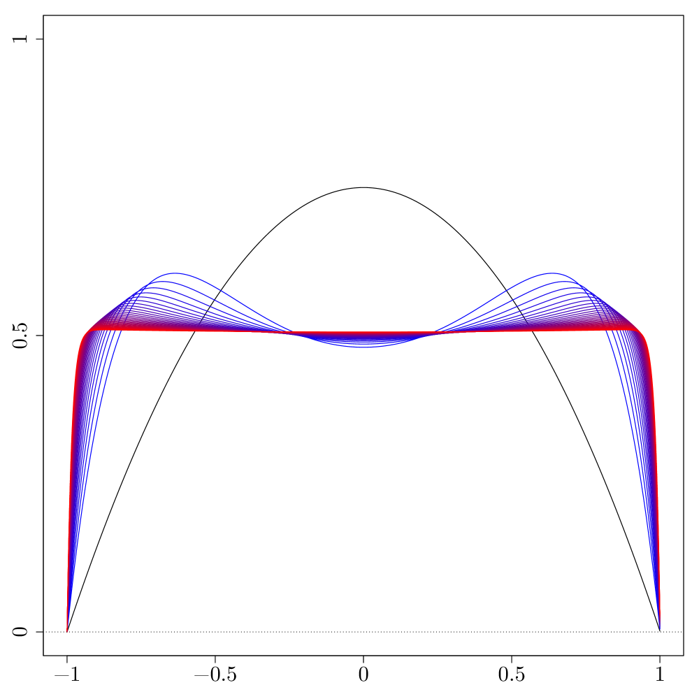
Figure 1: Equivalent Kernels of the Minimum Distance Density Estimators.

Notes. We set $P(u)=u$ or $P(u)=(u,u^{2}/2)^{\prime}$, and $K$ uniform. The redundant regressor is $Q(u)=u^{2j+1}$ for $j=1,2,\cdots,30$. The initial equivalent kernel is quadratic (black solid line), and the minimum variance kernel is uniform (red solid line).

Finally, in this paper we focus on minimizing the asymptotic variance of the estimator $\hat{\theta}$ and its variants because our main goal is inference. However, our results could be modified and extended to optimize the asymptotic mean square error (MSE). We do not pursue point estimation optimality further for brevity, but we do note that in the case of local polynomial density estimation (Cattaneo, Jansson, and Ma, 2020), the resulting estimator is automatically MSE-optimal at interior points when $p\leq 2$, because the induced equivalent kernel coincides with the Epanechnikov kernel (Granovsky and Müller, 1991; Cheng, Fan, and Marron, 1997).

4 Uniform Distribution Theory

The distributional result presented in Theorem 1 is valid pointwise for $\mathsf{x}\in\mathcal{X}$. We now develop an uniform distributional approximation for the Studentized process

$$\left\{T(\mathsf{x})=\frac{c^{\prime}\hat{\theta}(\mathsf{x})-c^{\prime}\theta(\mathsf{x})}{\sqrt{c^{\prime}\hat{\Omega}(\mathsf{x})c}}\ :\ \mathsf{x}\in\mathcal{I}\right\},$$

using the notation in (5), where $c$ is a conformable vector and $\mathcal{I}\subseteq\mathcal{X}$ is some prespecified region. This stochastic process is not asymptotically tight, and hence does not converge in distribution. Our approximation proceeds in two steps. First, for an positive (vanishing) sequence, $r_{\mathtt{L},n}$, we establish a uniform “linearization” of the process $T(\cdot)$ of the form:

$$\sup_{\mathsf{x}\in\mathcal{I}}\left|T(\mathsf{x})-\mathfrak{T}(\mathsf{x})\right|=O_{\mathbb{P}}(r_{\mathtt{L},n}),$$ (11)

where

$$\left\{\mathfrak{T}(\mathsf{x})=\frac{1}{\sqrt{n}}\sum_{i=1}^{n}\mathcal{K}_{h,\mathsf{x}}(x_{i})\ :\ \mathsf{x}\in\mathcal{I}\right\}$$

with

$$\mathcal{K}_{h,\mathsf{x}}(x_{i})=\frac{c^{\prime}\Upsilon_{h}\Gamma_{h,\mathsf{x}}^{-1}\int_{\mathcal{X}_{h}}R(u)\Big{[}\mathds{1}(x_{i}\leq\mathsf{x}+hu)-F(\mathsf{x}+hu)\Big{]}K\left(u\right)f(\mathsf{x}+hu)\mathrm{d}u}{\sqrt{c^{\prime}\Upsilon_{h}\Omega_{h,\mathsf{x}}\Upsilon_{h}c}},$$

and $\Omega_{h,\mathsf{x}}=\Gamma_{h,\mathsf{x}}^{-1}\Sigma_{h,\mathsf{x}}\Gamma_{h,\mathsf{x}}^{-1}$. In words, we show that the Studentized process $T(\cdot)$, which involves various pre-asymptotic estimated quantities, is uniformly close to the linearized process $\mathfrak{T}(\cdot)$, which is a sample average of independent observations. To obtain (11), we develop new uniform approximations with precise convergence rates, which may be of independent interest in semiparametric estimation and inference settings. See the SA for more details.

Second, in a possibly enlarged probability space, we show that there exists a copy of $\mathfrak{T}(\cdot)$, denoted by $\tilde{\mathfrak{T}}(\cdot)$, and a centered Gaussian process $\{\mathfrak{B}(\mathsf{x}):\mathsf{x}\in\mathcal{I}\}$, with a suitable variance-covariance structure, such that

$$\sup_{\mathsf{x}\in\mathcal{I}}\left|\tilde{\mathfrak{T}}(\mathsf{x})-\mathfrak{B}(\mathsf{x})\right|=O_{\mathbb{P}}(r_{\mathtt{G},n}),$$ (12)

where $r_{\mathtt{G},n}$ is another positive (vanishing) sequence. This type of strong approximation result, when established with suitably fast rate $r_{\mathtt{G},n}\to 0$, can be used to deduce distributional approximations for statistics such as $\sup_{\mathsf{x}\in\mathcal{I}}|T(\mathsf{x})|$, which are useful for constructing confidence bands or for conducting hypothesis tests about shape or other restrictions on the function of interest. To obtain (12), we employ a result established by Rio (1994), and later extended in Giné, Koltchinskii, and Sakhanenko (2004); see also (Giné and Nickl, 2010, Proof of their Proposition 5).

In this section we consider a fixed linear combination $c$ for ease of exposition, but in the SA we discuss the more general case where $c$ can depend on both the evaluation point $\mathsf{x}$ and the tuning parameter $h$, which is necessary to establish uniform distribution approximations for the minimum distance estimator introduced in Section 3.3. All the results reported in this section apply to the latter class of estimators as well.

4.1 Assumptions

In addition to Assumption 1, we impose the following conditions on the data generating process. In the sequel, continuity and differentiability conditions at boundary points should be interpreted as one-sided statements (i.e., as in part (i) of Assumption 1).

Assumption 2

Let $\mathcal{I}\subseteq\mathcal{X}$ be a compact interval.

(i) The density function $f(\mathsf{x})$ is twice continuously differentiable and bounded away from zero on $\mathcal{I}$.

(ii) There exists some $\delta>0$ and compactly supported kernel functions $K^{{\dagger}}(\cdot)$ and $\{K^{{\ddagger},d}(\cdot)\}_{d\leq\delta}$, such that (ii.1) $\sup_{u\in\mathbb{R}}|K^{{\dagger}}(u)|+\sup_{d\leq\delta,u\in\mathbb{R}}|K^{{\ddagger},d}(u)|<\infty$, (ii.2) the support of $K^{{\ddagger},d}(\cdot)$ has Lebesgue measure bounded by $Cd$, where $C$ is independent of $d$; and (ii.3) for all $u$ and $v$ such that $|u-v|\leq\delta$,

$$|K(u)-K(v)|\leq|u-v|\cdot K^{{\dagger}}(u)+K^{{\ddagger},|u-v|}(u).$$

(iii) The basis function $R(\cdot)$ is Lipschitz continuous in $[-1,1]$.

(iv) For all $h$ sufficiently small, the minimum eigenvalues of $\Gamma_{h,\mathsf{x}}$ and $h^{-1}\Sigma_{h,\mathsf{x}}$ are bounded away from zero uniformly for $\mathsf{x}\in\mathcal{I}$.

The above strengthens and expands Assumption 1. Part (i) requires the density function to be reasonably smooth uniformly in $\mathcal{I}$. Part (ii) imposes additional requirements on the kernel function. Although seemingly technical, it permits a decomposition of the difference $|K(u)-K(v)|$ into two parts. The first part, $|u-v|\cdot K^{{\dagger}}(u)$, is a kernel function which vanishes uniformly as $|u-v|$ becomes small. Note that this will be the case for all piecewise smooth kernel functions, such as the triangular or the Epanechnikov kernel. However, difference of discontinuous kernels, such as the uniform kernel, cannot be made uniformly close to zero. This motivates the second term in the above decomposition. Part (iii) requires the basis function to be reasonably smooth. Together, parts (i)–(iii) imply that the estimator $\hat{\theta}(\mathsf{x})$ will be “smooth” in $\mathsf{x}$, which is important to control the complexity of the process $T(\cdot)$. Finally, part (iv) implies that the matrices $\Gamma_{h,\mathsf{x}}$ and $\Sigma_{h,\mathsf{x}}$ are well-behaved uniformly for $\mathsf{x}\in\mathcal{I}$.

4.2 Strong Approximation

We first discuss the covariance of the process $\mathfrak{T}(\cdot)$. It is straightforward to show that

$$\mathbb{C}\mathrm{ov}[\mathfrak{T}(\mathsf{x}),\mathfrak{T}(\mathsf{y})]=\frac{c^{\prime}\Upsilon_{h}\Omega_{h,\mathsf{x},\mathsf{y}}\Upsilon_{h}c}{\sqrt{c^{\prime}\Upsilon_{h}\Omega_{h,\mathsf{x}}\Upsilon_{h}c}\sqrt{c^{\prime}\Upsilon_{h}\Omega_{h,\mathsf{y}}\Upsilon_{h}c}},\qquad\Omega_{h,\mathsf{x},\mathsf{y}}=\Gamma_{h,\mathsf{x}}^{-1}\Sigma_{h,\mathsf{x},\mathsf{y}}\Gamma_{h,\mathsf{y}}^{-1},$$

where

$$\Sigma_{h,\mathsf{x},\mathsf{y}}=\int_{\mathcal{X}_{h,\mathsf{y}}}\int_{\mathcal{X}_{h,\mathsf{x}}} R(u)R(v)^{\prime}\Big{[}F(\min\{\mathsf{x}+hu,\mathsf{y}+hv\})-F(\mathsf{x}+hu)F(\mathsf{y}+hv)\Big{]}$$

$$\cdot K(u)K(v)f(\mathsf{x}+hu)f(\mathsf{y}+hv)\mathrm{d}u\mathrm{d}v,$$

and $\Sigma_{h,\mathsf{x},\mathsf{x}}=\Sigma_{h,\mathsf{x}}$.

Now we state the second main distributional result of this paper in the following theorem.

Theorem 3 (Strong Approximation)

Suppose Assumptions 1 and 2 hold, and that $h\to 0$ and $nh^{2}/\log(n)\to\infty$.

1. (11) holds with

   $$r_{\mathtt{L},n}=\sqrt{\frac{n}{h}}\sup_{\mathsf{x}\in\mathcal{I}}\varrho(h,\mathsf{x})+\frac{\log(n)}{\sqrt{nh^{2}}}.$$

2. On a possibly enlarged probability space, there exists a copy $\tilde{\mathfrak{T}}(\cdot)$ of $\mathfrak{T}(\cdot)$, and a centered Gaussian process, $\{\mathfrak{B}(\mathsf{x}),\mathsf{x}\in\mathcal{I}\}$, defined with the same covariance as $\mathfrak{T}(\cdot)$, such that (12) holds with

   $$r_{\mathtt{G},n}=\frac{\log(n)}{\sqrt{nh}}.$$

The first part of this theorem gives conditions such that the feasible Studentized process $T(\cdot)$ is well approximated by the infeasible (linear) process $\mathfrak{T}(\cdot)$, uniformly for $\mathsf{x}\in\mathcal{I}$. The latter process is mean zero, and takes a kernel-based form. However, standard strong approximation results for kernel-type estimators do not apply directly to the process $\mathfrak{T}(\cdot)$, as the implied (equivalent, Studentized) kernel $\mathcal{K}_{h,\mathsf{x}}(\cdot)$ depends not only on the bandwidth but also on the evaluation point in a non-standard way. That is, due to the boundary adaptive feature of the local regression distribution estimators, the shape of the implied kernel automatically changes for different evaluation points depending on whether they are interior or boundary points.

Putting the two results together, it follows that the distribution of $T(\cdot)$ is approximated by that of $\mathfrak{B}(\cdot)$, provided the following condition holds:

$$\sqrt{\frac{n}{h}}\sup_{\mathsf{x}\in\mathcal{I}}\varrho(h,\mathsf{x})+\frac{\log(n)}{\sqrt{nh^{2}}}\to 0.$$

To facilitate understanding of this rate restriction, we consider the local polynomial density estimation setting of Cattaneo, Jansson, and Ma (2020), where the basis function takes the form $R(u)=(1,u,u^{2}/2,\cdots,u^{p}/p!)^{\prime}$ for some $p\geq 1$, and the second element of $\hat{\theta}(\mathsf{x})$ estimates the density $f(\mathsf{x})$. That is, $e_{1}^{\prime}\hat{\theta}(\mathsf{x})=\hat{f}(\mathsf{x})\to_{\mathbb{P}}f(\mathsf{x})$ under Assumption 1, where $c=e_{1}$. By a Taylor expansion argument, it is easy to see that the smoothing bias has order $h^{p+1}$ as long as the distribution function $F(\cdot)$ is suitably smooth. Then, the above rate restriction reduces to $\sqrt{nh^{2p+1}}+{\frac{\log(n)}{\sqrt{nh^{2}}}}\to 0$.

Finally, if the goal is to approximate the distribution of $\sup_{\mathsf{x}\in\mathcal{I}}|T(\mathsf{x})|$, then an extra $\sqrt{\log(n)}$ factor is needed in the rate restriction, as discussed in Chernozhukov, Chetverikov, and Kato (2014a). A formal statement of such result is given below, after we discuss how we can further approximate the infeasible Gaussian process $\mathfrak{B}(\cdot)$.

4.3 Confidence Bands

Feasible inference cannot be based on the Gaussian process $\mathfrak{B}(\cdot)$, as its covariance structure is unknown and has to be estimated in practice. For estimation, first recall from Sections 2 and 3 that $W_{i}(\mathsf{x})=K((x_{i}-\mathsf{x})/h)/h$, $R_{i}(\mathsf{x})=R(x_{i}-\mathsf{x})$, and $\hat{\Gamma}(\mathsf{x})=\frac{1}{n}\sum_{i=1}^{n}W_{i}(\mathsf{x})R_{i}(\mathsf{x})R_{i}(\mathsf{x})^{\prime}$. Then, we construct the plug-in estimator of $\Omega_{h,\mathsf{x},\mathsf{y}}$ as follows:

$$\hat{\Omega}_{h,\mathsf{x},\mathsf{y}}=n\Upsilon_{h}^{-1}\hat{\Gamma}(\mathsf{x})^{-1}\hat{\Sigma}(\mathsf{x},\mathsf{y})\hat{\Gamma}(\mathsf{y})^{-1}\Upsilon_{h}^{-1},\qquad\hat{\Sigma}(\mathsf{x},\mathsf{y})=\frac{1}{n^{2}}\sum_{i=1}^{n}\hat{\psi}_{i}(\mathsf{x})\hat{\psi}_{i}(\mathsf{y})^{\prime}$$

where

$$\hat{\psi}_{i}(\mathsf{x})=\frac{1}{n}\sum_{j=1}^{n}W_{j}(\mathsf{x})R_{j}(\mathsf{x})(\mathds{1}(x_{i}\leq x_{j})-\hat{F}_{j}).$$

The following theorem combines previous results, and justifies the uniform confidence band constructed using critical values from $\sup_{\mathsf{x}\in\mathcal{I}}|\hat{\mathfrak{B}}(\mathsf{x})|$. Let $X_{n}=(x_{1},x_{2},\dots,x_{n})^{\prime}$.

Theorem 4 (Kolmogorov-Smirnov Distance)

Suppose Assumptions 1 and 2 hold, and that $n\sup_{\mathsf{x}\in\mathcal{I}}\varrho(h,\mathsf{x})^{2}\log(n)/h+\log(n)^{5}/(nh^{2})\to 0$. Then, conditional on $X_{n}$, there exists a centered Gaussian process $\{\hat{\mathfrak{B}}(\mathsf{x}),\mathsf{x}\in\mathcal{I}\}$ with covariance

$$\mathbb{C}\mathrm{ov}\left[\left.\hat{\mathfrak{B}}(\mathsf{x}),\hat{\mathfrak{B}}(\mathsf{y})\right|X_{n}\right]=\frac{c^{\prime}\Upsilon_{h}\hat{\Omega}_{h,\mathsf{x},\mathsf{y}}\Upsilon_{h}c}{\sqrt{c^{\prime}\Upsilon_{h}\hat{\Omega}_{h,\mathsf{x}}\Upsilon_{h}c}\sqrt{c^{\prime}\Upsilon_{h}\hat{\Omega}_{h,\mathsf{y}}\Upsilon_{h}c}},$$

such that

$$\sup_{u\in\mathbb{R}}\left|\mathbb{P}\Big{[}\sup_{\mathsf{x}\in\mathcal{I}}|T(\mathsf{x})|\leq u\Big{]}-\mathbb{P}\Big{[}\sup_{\mathsf{x}\in\mathcal{I}}|\hat{\mathfrak{B}}(\mathsf{x})|\leq u\Big{|}X_{n}\Big{]}\right|=o_{\mathbb{P}}(1).$$

From Theorem 4, an asymptotically valid $100(1-\alpha)\%$ confidence band for $\{c^{\prime}{\theta}(\mathsf{x}):\mathsf{x}\in\mathcal{I}\}$ is given by

$$\text{CI}_{\alpha}(\mathcal{I})=\left\{\left[c^{\prime}\hat{\theta}(\mathsf{x})-\mathfrak{q}_{1-\alpha}\sqrt{c^{\prime}\hat{\Omega}(\mathsf{x})c}~{},~{}c^{\prime}\hat{\theta}(\mathsf{x})+\mathfrak{q}_{1-\alpha}\sqrt{c^{\prime}\hat{\Omega}(\mathsf{x})c}\right],\quad\mathsf{x}\in\mathcal{I}\right\},$$

where $\mathfrak{q}_{1-\alpha}$ is the $1-\alpha$ quantile of $\sup_{\mathsf{x}\in\mathcal{I}}|\hat{\mathfrak{B}}(\mathsf{x})|$, conditional on the data. That is,

$$\mathfrak{q}_{a}=\inf\left\{u\in\mathbb{R}:\mathbb{P}\left[\sup_{\mathsf{x}\in\mathcal{I}}|\hat{\mathfrak{B}}(\mathsf{x})|\leq u\Big{|}X_{n}\right]\geq a\right\},$$

which can be obtained by simulating the process $\hat{\mathfrak{B}}(\cdot)$ on a dense grid.

As an alternative to analytic estimation of the covariance kernel, it is possible to consider resampling methods as in Chernozhukov, Chetverikov, and Kato (2014a), Cheng and Chen (2019), Cattaneo, Farrell, and Feng (2020), and references therein. We relegate resampling-based inference for future research.

5 Extensions and Other Applications

We briefly outline some extensions of our main results. First, we introduce a re-weighted version of $\hat{\theta}$, which is useful in applications as illustrated in Section 6. Second, we discuss a new class of local regression estimators based on a non-random least-squares loss function, which has some interesting theoretical properties and may be of interest in some semiparametric settings. Finally, we discuss how to incorporate restrictions in the estimation procedure, employing the generic structure of the local basis $R(\cdot)$.

5.1 Re-weighted Distribution Estimator

Suppose $(x_{1},w_{1}),(x_{2},w_{2}),\cdots,(x_{n},w_{n})$ is a random sample, where $x_{i}$ is a continuous random variable with a smooth cumulative distribution function, but now $w_{i}$ is an additional “weighting” variable, possibly random and involving unknown parameters. We consider the generic weighted distribution parameter

$$H(\mathsf{x})=\mathbb{E}[w_{i}\mathds{1}(x_{i}\leq\mathsf{x})],$$

whose practical interpretation depends on the specific choice of $w_{i}$.

We discuss some examples. If $w_{i}=1$, $H(\cdot)$ becomes the distribution function $F(\cdot)$, and hence the results above apply. If $w_{i}$ is set to be a certain ratio of propensity scores for subpopulation membership, then the derivative $\mathrm{d}H(\mathsf{x})/\mathrm{d}\mathsf{x}$ becomes a counterfactual density function, as in DiNardo, Fortin, and Lemieux (1996); see Section 6.1 below. If $w_{i}$ is set to be a combination of the treatment assignment and treatment status variables, then the resulting derivative can be used to conduct specification testing in IV models, or if $w_{i}$ is set to be a certain ratio of propensity scores for a binary instrument, then the derivative can be used to identify distributions of compliers, as in Imbens and Rubin (1997), Abadie (2003), and Kitagawa (2015); see Section 6.2 below. Other examples of applicability of this extension include bunching, missing data, measurement error, data combination, and treatment effect settings.

More generally, when weights are allowed for, there is another potentially interesting connection between the estimand $\mathrm{d}H(\mathsf{x})/\mathrm{d}\mathsf{x}$ and classical weighted averages featuring prominently in econometrics because $\mathrm{d}H(\mathsf{x})/\mathrm{d}\mathsf{x}=\mathbb{E}[w_{i}|x_{i}=\mathsf{x}]f(\mathsf{x})$, which is useful in the context of partial means and related problems as in Newey (1994b).

Our main results extend immediately to allow for $\sqrt{n}$-consistent estimated weights $w_{i}$ or, more generally, to estimated weights that converge sufficiently fast. Specifically, we let $\hat{F}_{w,i}(x)=\frac{1}{n}\sum_{j=1}^{n}w_{j}\mathds{1}(x_{j}\leq x)$ in place of $\hat{F}_{i}$, and investigate the large sample properties of our proposed estimator in (2) when $w_{i}$ is replaced by $\hat{w_{i}}=w_{i}(\hat{\beta})$ with $\hat{\beta}$ an $a_{n}$-consistent estimator, for some $a_{n}\to\infty$, and $w_{i}(\cdot)$ a known function of the data. That is, when estimated weights are used to construct the weighted empirical distribution function $\hat{F}_{w,i}(x)$. Provided that $a_{n}^{-1}\to 0$ sufficiently fast, this extra estimation step will not affect the asymptotic properties of our estimator of the density function or its derivatives (which will be true, for example, in parametric estimation cases, where $a_{n}=\sqrt{n}$ under regularity conditions). All the results reported in the previous sections apply to this extension, which we illustrate empirically below.

5.2 Local $L^{2}$ Distribution Estimators

The local regression distribution estimator is obtained from a least squares projection of the empirical distribution function onto a local basis, where the projection puts equal weights at all observations. That is, (2) employs an $L^{2}(\hat{F})$-projection

$$\hat{\theta}(\mathsf{x})=\operatorname*{argmin}_{\theta}\int\Big{(}\hat{F}(u)-R(u-\mathsf{x})^{\prime}\theta\Big{)}^{2}K\left(\frac{u-\mathsf{x}}{h}\right)\mathrm{d}\hat{F}(u).$$

This representation motivates a general class of local $L^{2}$ distribution estimators given by

$$\hat{\theta}_{G}(\mathsf{x})=\operatorname*{argmin}_{\theta}\int\Big{(}\hat{F}(u)-R(u-\mathsf{x})^{\prime}\theta\Big{)}^{2}K\left(\frac{u-\mathsf{x}}{h}\right)\mathrm{d}G(u)$$

for some measure $G$. We show in the SA that all our theoretical results continue to hold for $\hat{\theta}_{G}$, provided that $G$ is absolutely continuous with respect to the Lebesgue measure and the Radon-Nikodym derivative is reasonably smooth. (Note that $G$ does not need to be a proper distribution function.)

The estimator $\hat{\theta}_{G}$ involves only one average, while the local regression estimator $\hat{\theta}$ has two layers of averages (one from the construction of the empirical distribution function, and the other from the $L^{2}(\hat{F})$-projection/regression). As a result, with suitable centering and scaling, the local $L^{2}$ distribution estimator, $\hat{\theta}_{G}$, can be written as the sum of a mean-zero influence function and a smoothing bias term. Since $\hat{\theta}_{G}$ no longer involves a second order U-statistic (c.f. (6)), or a leave-in bias, pointwise asymptotic normality can be established under weaker conditions: it is no longer needed to assume $nh^{2}\to\infty$ (Theorem 1), and $nh\to\infty$ will suffice. Similarly, for the strong approximation results we only need to restrict $\log(n)/\sqrt{nh}$ as opposed to $\log(n)/\sqrt{nh^{2}}$ (part 1 of Theorem 3).

In addition, the local $L^{2}$ distribution estimator $\hat{\theta}_{G}$ is robust to “low” density. To see this, recall that the local regression estimator $\hat{\theta}$ involves regressing the empirical distribution on a local basis, which means that this estimator can be numerically unstable if there are only a few observations near the evaluation point. More precisely, the matrix $\hat{\Gamma}$ will be close to singular if the effective sample size is small.

Although the local $L^{2}$ distribution estimator $\hat{\theta}_{G}$ takes a simpler form, is robust to low density, and its large sample properties can be established under weaker bandwidth conditions, it does have one drawback: it requires knowledge of the support $\mathcal{X}$. To be more precise, let $G$ be the Lebesgue measure, then the local $L^{2}$ distribution estimator may be biased at or near boundaries of $\mathcal{X}$ if it is compact. In contrast, the local regression distribution estimator is fully boundary adaptive, even in cases where the location of the boundary is unknown. See Cattaneo, Jansson, and Ma (2020) for further discussion for the case of density estimation.

5.3 Incorporating Restrictions

The formulation (2) is general enough to allow for some interesting extensions in the definition of the local regression distribution estimator. The key observation is that the estimator has a weighted least squares representation with a generic local basis function $R(\cdot)$, which allows for deploying well-know results from linear regression models. We briefly illustrate this idea with three examples.

First, consider the case where the local basis $R(u)$ incorporates specific restrictions, such as continuity or lack thereof, on the distribution function, density function or higher-order derivatives at the evaluation point $\mathsf{x}$. To give a concrete example, suppose that $F(\mathsf{x})$ and $f(\mathsf{x})$ are known to be continuous at some interior point $\mathsf{x}\in\mathcal{X}$, while no information is available for the higher-order derivatives. Then, these restriction can be effortlessly incorporated to the local regression distribution estimator by considering the local basis function

$$R(u)=\left(1,u,\frac{u^{2}}{2}\mathds{1}(u<\mathsf{x}),\frac{u^{2}}{2}\mathds{1}(u\geq\mathsf{x}),\frac{u^{3}}{6}\mathds{1}(u<\mathsf{x}),\frac{u^{3}}{6}\mathds{1}(u\geq\mathsf{x}),\cdots,\frac{u^{p}}{p!}\mathds{1}(u<\mathsf{x}),\frac{u^{p}}{p!}\mathds{1}(u\geq\mathsf{x})\right)^{\prime}.$$

It follows that $\hat{f}(\mathsf{x})=e_{1}^{\prime}\hat{\theta}(\mathsf{x})$ consistently estimates the density $f(\mathsf{x})$ at the kink point $\mathsf{x}$, while $e_{2}^{\prime}\hat{\theta}(\mathsf{x})$ and $e_{3}^{\prime}\hat{\theta}(\mathsf{x})$ are consistent estimators of the left and the right derivatives of the density function, respectively (and similarly for other higher-order one-sided derivatives). In this example, the generalized formulation not only reduces the bias of $\hat{f}(\mathsf{x})=e_{1}^{\prime}\hat{\theta}(\mathsf{x})$ even in the absence of continuity of higher-order derivatives, but also provides the basis for testing procedures for continuity of higher-order derivatives; e.g., by considering an statistic based on $(e_{2}-e_{3})^{\prime}\hat{\theta}(\mathsf{x})$. This provides a concrete illustration of the advantages of allowing for generic local basis. A distinct example was developed in Cattaneo, Jansson, and Ma (2018, 2020) for density discontinuity testing in regression discontinuity designs.

As a second example, consider imposing shape constraints, such as positivity or monotonicity, in the construction of the local regression distribution estimator. Such constraints amount to specific restrictions on the parameter space of $\theta$, which naturally leads to restricted weighted least squares estimation in the context of our estimator. To be concrete, consider constructing a local polynomial density estimator which is non-negative, in which case $R(u)$ is a polynomial basis of order $p\geq 1$ and (2) is extended to:

$$\hat{\theta}(\mathsf{x})= \operatorname*{argmin}_{\theta}\sum_{i=1}^{n}W_{i}(\hat{F}_{i}-R_{i}^{\prime}\theta)^{2}\qquad\text{subject to }T\theta\geq 0,$$

where $T$ denotes a matrix of restrictions; in this example, $T=e_{1}^{\prime}$ to ensure that $\hat{f}(\mathsf{x})=e_{1}^{\prime}\hat{\theta}(\mathsf{x})\geq 0$. This example showcases the advantages of the weighted least squares formulation of our estimator. Local monotonicity constraints, for instance, could also be easily incorporated in a similar fashion.

The final example of extensions of our basic local regression distribution estimation approach concerns non-identity link functions, leading to a non-linear least squares formulation. Specifically, (2) can be generalized to $\hat{\theta}(\mathsf{x})=\operatorname*{argmin}_{\theta}\sum_{i=1}^{n}W_{i}(\hat{F}_{i}-\Lambda(R_{i}^{\prime}\theta))^{2}$ for some known link function $\Lambda(\cdot)$. For instance, such extension may be useful to model distributions with large support or to impose specific local shape constraints.

All of the examples above, as well as many others, can be analyzed using the large sample results developed in this paper and proper extensions thereof. We plan to investigate these and other extensions in future research.

6 Applications

We discuss two applications of our main results in the context of program evaluation (see Abadie and Cattaneo, 2018, and references therein).

6.1 Counterfactual Densities

In this first application, the objects of interest are density functions over their entire support, including boundaries and near-boundary regions, which are estimated using estimated weighting schemes, as this is a key feature needed for counterfactual analysis (and many other applications). Our general estimation strategy is specialized to the counterfactual density approach originally proposed by DiNardo, Fortin, and Lemieux (1996). We focus on density estimation, and we refer readers to Chernozhukov, Fernandez-Val, and Melly (2013) for related methods based on distribution functions as well as for an overview of the literature on counterfactual analysis.

To construct a counterfactual density or, more generally, re-weighted density estimators, we simply need to set the weights $(w_{1},w_{2},\cdots,w_{n})$ appropriately. In most applications, this also requires constructing preliminary consistent estimators of these weights, as we illustrate in this section. Suppose the observed data is $(x_{i},t_{i},{z}_{i}^{\prime})^{\prime}$, $i=1,2,\dots,n$, where $x_{i}$ continues to be the main outcome variable, ${z}_{i}$ collects other covariates, and $t_{i}$ is a binary variable indicating to which group unit $i$ belongs. For concreteness, we call these two groups control and treatment, though our discussion does not need to bear any causal interpretation.

The marginal distribution of the outcome variable $x_{i}$ for the full sample can be easily estimated without weights (that is, $w_{i}=1$). In addition, two conditional densities, one for each group, can be estimated using $w^{1}_{i}=t_{i}/\mathbb{P}[t_{i}=1]$ for the treatment group and $w^{0}_{i}=(1-t_{i})/\mathbb{P}[t_{i}=0]$ for the control group, and are denote by $\hat{f}_{1}(x)$ and $\hat{f}_{0}(x)$, respectively. For example, in the context of randomized controlled trials, these density estimators can be useful to depict the distribution of the outcome variables for control and treatment units.

A more challenging question is: what would the outcome distribution have been, had the treated units had the same covariates distribution as the control units? The resulting density is called the counterfactual density for the treated, which is denoted by $f_{1\rhd 0}(x)$. Knowledge about this distribution is important for understanding differences between $f_{1}(x)$ and $f_{0}(x)$, as the outcome distribution is affected by both group status and covariates distribution. Furthermore, the counterfactual distribution has another useful interpretation: Assume the outcome variable is generated from potential outcomes, $x_{i}=t_{i}x_{i}(1)+(1-t_{i})x_{i}(0)$, then under unconfoundedness, that is, assuming $t_{i}$ is independent of $(x_{i}(0),x_{i}(1))^{\prime}$ conditional on the covariates ${z}_{i}$, $f_{1\rhd 0}(x)$ is the counterfactual distribution for the control group: it is the density function associated with the distribution of $x_{i}(1)$ conditional on $t_{i}=0$.

Regardless of the interpretation taken, $f_{1\rhd 0}(x)$ is of interest and can be estimated using our generic density estimator $\hat{f}(x)$ with the following weights:

$$w^{1\rhd 0}_{i}=t_{i}\cdot\frac{\mathbb{P}[t_{i}=0|{z}_{i}]}{\mathbb{P}[t_{i}=1|{z}_{i}]}\frac{\mathbb{P}[t_{i}=1]}{\mathbb{P}[t_{i}=0]}.$$

In practice, this choice of weighting scheme is unknown because the conditional probability $\mathbb{P}[t_{i}=1|{z}_{i}]$, a.k.a. the propensity score, is not observed. Thus, researchers estimate this quantity using a flexible parametric model, such as Probit or Logit. Our technical results allow for these estimated weights to form counterfactual density estimators after replacing the theoretical weights by their estimated counterparts, provided the estimated weights converge sufficiently fast to their population counterparts.

To be more precise, we can model $\mathbb{P}[t_{i}=1|{z}_{i}]=G(b(z_{i})^{\prime}\beta)$ for some known link function $G(\cdot)$, such as Logit or Probit, and $K$-dimensional basis expansion $b(z_{i})$, such as power series or B-splines. If the model is correctly specified for some fixed $K$ and basis function $b(\cdot)$, then $\max_{1\leq i\leq n}|w_{i}-\hat{w_{i}}|=O_{\mathbb{P}}(a^{-1}_{n})$ with $a_{n}=\sqrt{n}$ under mild regularity conditions, and all our results carry over to the setting with estimated weights mentioned in Section 5.1. Alternatively, from a nonparametric perspective, if $K\to\infty$ as $n\to\infty$, and for appropriate basis function $b(\cdot)$ and regularity conditions, $\max_{1\leq i\leq n}|w_{i}-\hat{w_{i}}|=O_{\mathbb{P}}(a^{-1}_{n})$ with $a_{n}$ depending on both $K$ and $n$. Then, as in the parametric case, our main results carry over if $a_{n}^{-1}\to 0$ fast enough. The exact rate requirements can be deduced from the main theorems above.

6.1.1 Empirical Illustration

We demonstrate empirically how marginal, conditional, and counterfactual densities can be estimated with our proposed method. We consider the effect of education on earnings using a subsample of the data in Abadie, Angrist, and Imbens (2002). The data consists of individuals who did not enroll in the Job Training Partnership Act (JTPA). The main outcome variable is the sum of earnings in a 30-month period, and individuals are split into two groups according to their education attainment: $t_{i}=1$ for those with high school degree or GED, and $t_{i}=0$ otherwise. Also available are demographic characteristics, including gender, ethnicity, age, marital status, AFDC receipt (for women), and a dummy indicating whether the individual worked at least 12 weeks during a one-year period. The sample size is $5,447$, with $3,927$ being either high school graduates or GED. Summary statistics are available as the fourth column in Table 1. We leave further details on the JTPA program to Section 6.2, where we utilize a larger sample and conduct distribution estimation in a randomized controlled (intention-to-treat) and instrumental variables (imperfect compliance) setting.

Table 1: Summary Statistics for the JTPA data.

	Full		JTPA Offer			JTPA Enrollment
			N	Y		N	Y
Income	$17949.20$		$17191.13$	$18321.59$		$17015.58$	$19098.44$
HS or GED	$0.72$		$0.71$	$0.72$		$0.70$	$0.74$
Male	$0.46$		$0.47$	$0.46$		$0.48$	$0.45$
Nonwhite	$0.36$		$0.36$	$0.36$		$0.36$	$0.37$
Married	$0.28$		$0.27$	$0.29$		$0.27$	$0.29$
Work $\leq$ 12	$0.44$		$0.43$	$0.44$		$0.44$	$0.44$
AFDC	$0.17$		$0.17$	$0.17$		$0.16$	$0.19$
Age
22-25	$0.24$		$0.25$	$0.24$		$0.24$	$0.25$
26-29	$0.21$		$0.20$	$0.21$		$0.21$	$0.21$
30-35	$0.24$		$0.25$	$0.24$		$0.24$	$0.25$
36-44	$0.19$		$0.19$	$0.19$		$0.20$	$0.19$
45-54	$0.08$		$0.08$	$0.08$		$0.08$	$0.07$
Sample Size	$9872$		$3252$	$6620$		$5447$	$4425$

Columns : (i) Full: full sample; (ii) JTPA Offer: whether offered JTPA services; (iii) JTPA Enrollment: whether enrolled in JTPA. Rows : (i) Income: cumulative income over 30-month period post random selection; (ii) HS or GED: whether has high school degree or GED; (iii) Male: gender being male; (iv) Nonwhite: black or Hispanic; (v) Married: whether married; (vi) Work $\leq$ 12: worked less than 12 weeks during one year period prior to random assignment; (vii) Age: age groups.

It is well-known that education has significant impact on labor income, and we first plot earning distributions separately for subsamples with and without high school degree or GED. The two estimates, $\hat{f}_{1}(x)$ and $\hat{f}_{0}(x)$, are plotted in panel (a) of Figure 2. There, it is apparent that the earning distribution for high school graduates is very different compared to those without high school degree. More specifically, both the mean and median of $\hat{f}_{1}(x)$ are higher than $\hat{f}_{0}(x)$, and $\hat{f}_{1}(x)$ seems to have much thinner left tail and thicker right tail.

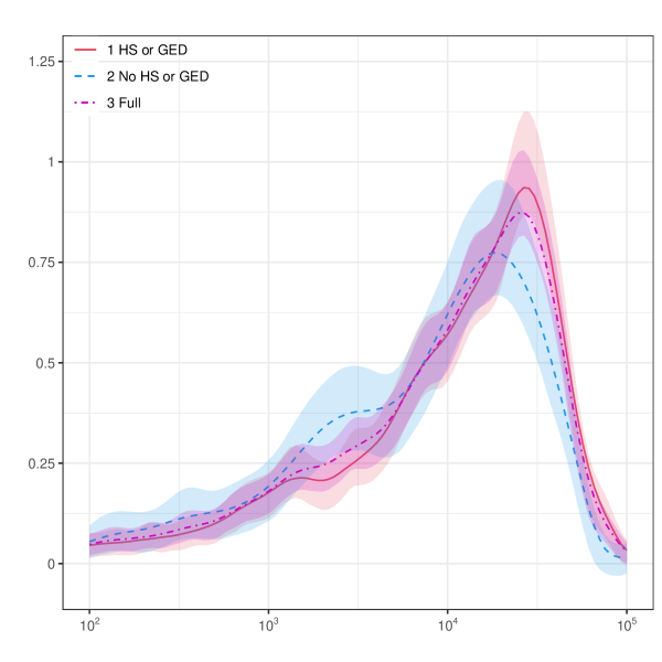
(a) Marginal Distributions

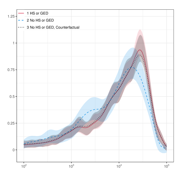
(b) Counterfactual Distribution

Figure 2: Earning Distributions by Education, JTPA.

Notes: (i) Full: earning distribution for the full sample ($n=5,447$); (ii) HS or GED: earning distributions for subgroups with and without high school degree or GED ($n=1,520$ and $3,927$, respectively); (iii) No HS or GED, Counterfactual: counterfactual earning distribution. Point estimates are obtained by using local polynomial regression with order 2, and robust confidence intervals are obtained with local polynomial of order 3. Bandwidths are chosen by minimizing integrated mean squared errors. All estimates are obtained using companion R (and Stata) package described in Cattaneo, Jansson, and Ma (2021).

As mentioned earlier, direct comparison between $\hat{f}_{1}(x)$ and $\hat{f}_{0}(x)$ does not reveal the impact of having high school degree on earning, since the difference is confounded by the fact that individuals with high school degree can have very different characteristics (measured by covariates) compared to those without. We employ covariates adjustments, and ask the following question: what would the earning distribution have been for high school graduates, had they had the same characteristics as those without such degree?

We estimate the counterfactual distribution $f_{1\rhd 0}(x)$ by our proposed method, and is shown in panel (b) of Figure 2. The difference between $\hat{f}_{1\rhd 0}(x)$ and $\hat{f}_{1}(x)$ is not very profound, although it seems $\hat{f}_{1\rhd 0}(x)$ has smaller mean and median. On the other hand, difference between $\hat{f}_{0}(x)$ and $\hat{f}_{1\rhd 0}(x)$ remains highly nontrivial. Our empirical finding is compatible with existing literature on return to education: it is generally believed that education leads to significant accumulation of human capital, hence increase in labor income. As a result, educational attainment is usually one of the most important “explanatory variables” for differences in income.

6.2 IV Specification and Heterogeneity

Self-selection and treatment effect heterogeneity are important concerns in causal inference and studies of socioeconomic programs. It is now well understood that classical treatment parameters, such as the average treatment effect or the treatment effect on the treated, are not identifiable even when treatment assignment is fully randomized due to imperfect compliance. Indeed, what can be recovered is either an intention-to-treat parameter or, using the instrumental variables method, some other more local treatment effect, specific to a subpopulation: the “compliers.” See Imbens and Rubin (2015) and references therein for further discussion. Practically, this poses two issues for empirical work employing instrumental variables methods focusing on local average treatment effects. First, since compliers are usually not identified, it is crucial to understand how different their characteristics are compared to the population as a whole. Second, it is often desirable to have a thorough estimate of the distribution of potential outcomes, which provides information not only on the mean or median, but also its dispersion, overall shape, or local curvatures.

Motivated by these observations, and to illustrate the applicability of our density estimation methods, we now consider two related problems. First, we investigate specification testing in the context of local average treatment effects based on comparison of two (rescaled) densities as discussed by Kitagawa (2015). This method requires estimating two densities nonparametrically. Second, we consider estimating the density of potential outcomes for compliers in the IV setting of Abadie (2003), which allows for conditioning on covariates. The resulting density plots not only provide visual guides on treatment effects, but also can be used for further analysis to construct a rich set of summary statistics or as inputs for semiparametric procedures. Both methods require estimated weights.

We first introduce the notation and the potential outcomes framework. For each individual there is a binary indicator of treatment assignment (a.k.a. the instrument), denoted by $d_{i}$. The actual treatment (takeup), however, can be different, due to imperfect compliance. More specifically, let $t_{i}(0)$ and $t_{i}(1)$ be the two potential treatments, corresponding to $d_{i}=0$ and $1$, then the observed binary treatment indicator is $t_{i}=d_{i}t_{i}(1)+(1-d_{i})t_{i}(0)$. We also have a pair of potential outcomes, $x_{i}(0)$ and $x_{i}(1)$, associated with $t_{i}=0$ and $1$, and what is observed is $x_{i}=t_{i}x_{i}(1)+(1-t_{i})x_{i}(0)$. Finally, also available are some covariates, collected in ${z}_{i}$. We assume that the observed data is a random sample $\{(x_{i},t_{i},d_{i},{z}_{i}^{\prime})^{\prime}:1\leq i\leq n\}$.

There are three important assumptions for identification. First, the instrument has to be exogenous, meaning that conditional on covariates, it is independent of the potential treatments and outcomes. Second, the instrument has to be relevant, meaning that conditional on covariates, the instrument should be able to induce changes in treatment takeups. Third, there are no defiers (a.k.a. the monotonicity assumption). We do not reproduce the exact details of those assumptions and other technical requirements for identification; see the references given for more details.

Building on Imbens and Rubin (1997), Kitagawa (2015) discusses interesting testable implications in this IV setting, which can be easily adapted to test instrument validity using our density estimator. In the current context, the testable implications take the following form: for any (measurable) set $\mathcal{I}\subset\mathbb{R}$,

$$\mathbb{P}[x_{i}\in\mathcal{I},\ t_{i}=1|d_{i}=1]\geq\mathbb{P}[x_{i}\in\mathcal{I},\ t_{i}=1|d_{i}=0],$$

and $$\mathbb{P}[x_{i}\in\mathcal{I},\ t_{i}=0|d_{i}=0]\geq\mathbb{P}[x_{i}\in\mathcal{I},\ t_{i}=0|d_{i}=1].$$

The first requirement holds trivially in the JTPA context, since the program does not allow enrollment without being offered (that is, $\mathbb{P}[t_{i}=1|d_{i}=0]=0$). Therefore we demonstrate the second with our density estimator. Let $f_{d=0,t=0}(x)$ be the earning density for the subsample $d_{i}=0$ and $t_{i}=0$, that is, for individuals without JTPA offer and not enrolled. Similarly let $f_{d=1,t=0}(x)$ be the earning density for individuals offered JTPA but not enrolled. Then the second inequality in the above display is equivalent to, for all $x\in\mathbb{R}$,

$$\mathbb{P}[t_{i}=0|d_{i}=0]\cdot f_{d=0,t=0}(x)\geq\mathbb{P}[t_{i}=0|d_{i}=1]\cdot f_{d=1,t=0}(x).$$

Thus, our density estimator can be used directly, where $f_{d=0,t=0}(x)$ is consistently estimated with weights $w_{i}^{d=0,t=0}=(1-d_{i})(1-t_{i})/\mathbb{P}[d_{i}=0,t_{i}=0]$, and $f_{d=1,t=0}(x)$ is consistently estimated with $w_{i}^{d=1,t=0}=d_{i}(1-t_{i})/\mathbb{P}[d_{i}=1,t_{i}=0]$.

Abadie (2003) showed that the distributional characteristics of compliers are identified, and can be expressed as re-weighted marginal quantities. We focus on three distributional parameters here. The first one is the distribution of the observed outcome variable, $x_{i}$, for compliers, which is denoted by $f_{c}$. This parameter is important for understanding the overall characteristics of compliers, and how different it is from the populations. The other two parameters are distributions of the potential outcomes, $x_{i}(0)$ and $x_{i}(1)$, for compliers, since the difference thereof reveals the effect of treatment for this subgroup. They are denoted by $f_{c,0}$ and $f_{c,1}$, respectively. The three density functions can also be estimated using our proposed local polynomial density estimator $\hat{f}(x)$ with, respectively, the following weights:

$$w^{c}_{i} =\frac{1}{\mathbb{P}[t_{i}(1)>t_{i}(0)]}\cdot\left(1-\frac{t_{i}(1-d_{i})}{\mathbb{P}[d_{i}=0|{z}_{i}]}-\frac{(1-t_{i})d_{i}}{\mathbb{P}[d_{i}=1|{z}_{i}]}\right),$$

$$w^{c,0}_{i} =\frac{1}{\mathbb{P}[t_{i}(1)>t_{i}(0)]}\cdot(1-t_{i})\cdot\frac{1-d_{i}-\mathbb{P}[d_{i}=0|{z}_{i}]}{\mathbb{P}[d_{i}=0|{z}_{i}]\mathbb{P}[d_{i}=1|{z}_{i}]},$$

$$w^{c,1}_{i} =\frac{1}{\mathbb{P}[t_{i}(1)>t_{i}(0)]}\cdot t_{i}\cdot\frac{d_{i}-\mathbb{P}[d_{i}=1|{z}_{i}]}{\mathbb{P}[d_{i}=0|{z}_{i}]\mathbb{P}[d_{i}=1|{z}_{i}]}.$$

Here, the weights need to be estimated in practice, unless precise knowledge about the treatment assignment mechanism is available. As mentioned previously, our results allow for estimated weights such as those obtained by fitting a flexible Logit or Probit model to approximate the propensity score $\mathbb{P}[d_{i}=1|{z}_{i}]$ so long as they converge sufficiently fast to their population counterparts.

6.2.1 Empirical Illustration

The JTPA is a large publicly funded job training program targeting at individuals who are economically disadvantaged and/or facing significant barriers to employment. Individuals were randomly offered JTPA training, the treatment take-up, however, was only about 67% among those who were offered. Therefore the JTPA offer provides valid instrument to study the impact of the job training program. We continue to use the same data as Abadie, Angrist, and Imbens (2002), who analyzed quantile treatment effects on earning distributions.

Besides the main outcome variable and covariates already introduced in Section 6.1, also available are the treatment take-up (JTPA enrollment) and the instrument (JTPA Offer). See Table 1 for summary statistics for the full sample and separately for subgroups. As the JTPA offers were randomly assigned, it is possible to estimate the intent-to-treat effect by mean comparison. Indeed, individuals who are offered JTPA services earned, on average, $\$1,130$ more than those not offered. On the other hand, due to imperfect compliance, it is in general not possible to estimate the effect of job training (i.e. the effect of JTPA enrollment), unless one is willing to impose strong assumptions such as constant treatment effect.

We first implement the IV specification test, which is straightforward using our density estimator $\hat{f}(x)$. We plot the two estimated (rescaled) densities in Figure 3. A simple eyeball test suggests no evidence against instrumental variable validity. A formal hypothesis test, justified using our theoretical results, confirms this finding.

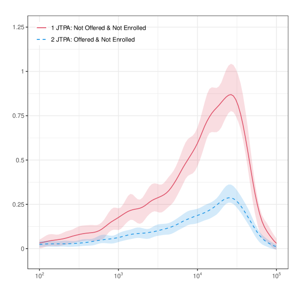
Figure 3: Testing Validity of Instruments, JTPA.

Notes : (i) JTPA: Not Offered & Not Enrolled: the scaled density estimate $\frac{\sum_{i}\mathds{1}(t_{i}=0,d_{i}=0)}{\sum_{i}\mathds{1}(d_{i}=0)}\hat{f}_{d=0,t=0}(x)$; (ii) JTPA: Offered & Not Enrolled: the scaled density estimate $\frac{\sum_{i}\mathds{1}(t_{i}=0,d_{i}=1)}{\sum_{i}\mathds{1}(d_{i}=1)}\hat{f}_{d=1,t=0}(x)$. Point estimates are obtained by using local polynomial regression with order 2, and robust confidence bands are obtained with local polynomial of order 3. Bandwidths are chosen by minimizing integrated mean squared errors. All estimates are obtained using companion R (and Stata) package described in Cattaneo, Jansson, and Ma (2021).

Second, we estimate the density of the potential outcomes for compliers. In panel (a) of Figure 4, we plot earning distributions for the full sample and that for the compliers, where the second is estimated using the weights $w_{i}^{c}$, introduced earlier. The two distributions seem quite similar, while compliers tend to have higher mean and thinner left tail in the earning distribution. Next we consider the intent-to-treat effect, as the difference in earning distributions for subgroups with and without JTPA offer (a.k.a. the reduced form estimate in the 2SLS context). This is given in panel (b) of Figure 4. The effect is significant, albeit not very large. We also plot earning distributions for individuals enrolled (and not) in JTPA in panel (c). Not surprisingly, the difference is much larger. Simple mean comparison implies that enrolling in JTPA is associated with $\$2,083$ more income.

(a) Marginal Distributions

(b) Marginal Distributions

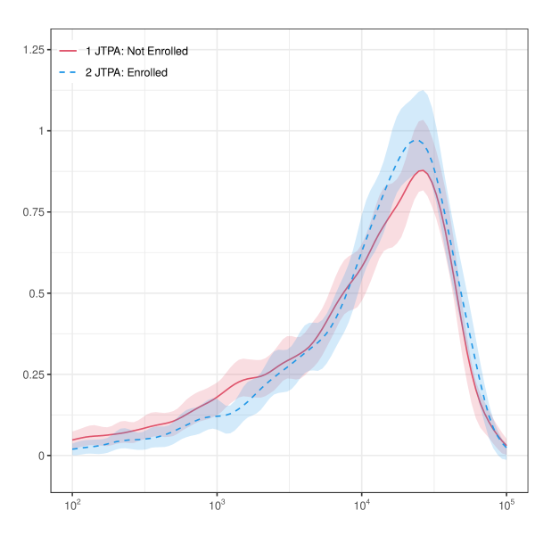
(c) Marginal Distributions

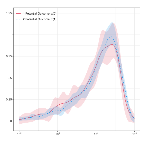
(d) Potential Outcome Distributions

Figure 4: Earning Distributions, JTPA.

Notes: (a) earning distributions in the full sample and for compliers; (b) earning distributions by JTPA offer; (c) earning distributions by JTPA enrollment; (d) distributions of potential outcomes for compliers. Point estimates are obtained by using local polynomial regression with order 2, and robust confidence bands are obtained with local polynomial of order 3. Bandwidths are chosen by minimizing integrated mean squared errors. All estimates are obtained using companion R (and Stata) package described in Cattaneo, Jansson, and Ma (2021).

Unfortunately, neither panel (b) nor (c) reveals information on distribution of potential outcomes. To see the reason, note that in panel (b) earning distributions are estimated according to treatment assignment, but potential outcomes are defined according to treatment takeup. And panel (c) does not give potential outcome distributions since treatment takeup is not randomly assigned. In panel (d) of Figure 4, we use weighting schemes $w_{i}^{c,0}$ and $w_{i}^{c,1}$ to construct potential earning distributions for compliers, which estimates the identified distributional treatment effect in this IV setting. Indeed, treatment effect on compliers is larger than the intent-to-treat effect, but is smaller than that in panel (c). The result is compatible with the fact that JTPA has positive and nontrivial effect on earning. Moreover, it demonstrates the presence of self-selection: those who participated in JTPA on average would benefit the most, followed by compliers who are regarded as “on the margin of indifference.”

7 Conclusion

We introduced a new class of local regression distribution estimator, which can be used to construct distribution, density, and higher-order derivatives estimators. We established valid large sample distributional approximations, both pointwise and uniform over their support. Pointwise on the evaluation point, we characterized a minimum distance implementation based on redundant regressors leading to asymptotic efficiency improvements, and gave precise results in terms of (tight) lower bounds for interior points. Uniformly over the evaluation points, we obtained valid linearizations and strong approximations, and constructed confidence bands. Finally, we discussed several extensions of our work.

Although beyond the scope of this paper, it would be useful to generalize our results to the case of multivariate regressors $x_{i}\in\mathbb{R}^{d}$. Boundary adaptation is substantially more difficult in multiple dimensions, and hence our proposed methods are potentially very useful in such setting. In addition, multidimensional density estimation can be used to construct new conditional distribution, density and higher derivative estimators in a straightforward way. These new estimators would be useful in several areas of economics, including for instance estimation of auction models.

References

- (1)
- Abadie (2003) Abadie, A. (2003): “Semiparametric Instrumental Variable Estimation of Treatment Response Models,” Journal of Econometrics, 113(2), 231–263.
- Abadie, Angrist, and Imbens (2002) Abadie, A., J. Angrist, and G. Imbens (2002): “Instrumental Variables Estimates of the Effect of Subsidized Training on the Quantiles of Trainee Earnings,” Econometrica, 70(1), 91–117.
- Abadie and Cattaneo (2018) Abadie, A., and M. D. Cattaneo (2018): “Econometric Methods for Program Evaluation,” Annual Review of Economics, 10, 465–503.
- Belloni, Chernozhukov, Chetverikov, and Fernandez-Val (2019) Belloni, A., V. Chernozhukov, D. Chetverikov, and I. Fernandez-Val (2019): “Conditional Quantile Processes based on Series or Many Regressors,” Journal of Econometrics, 213(1), 4–29.
- Belloni, Chernozhukov, Chetverikov, and Kato (2015) Belloni, A., V. Chernozhukov, D. Chetverikov, and K. Kato (2015): “Some New Asymptotic Theory for Least Squares Series: Pointwise and Uniform Results,” Journal of Econometrics, 186(2), 345–366.
- Calonico, Cattaneo, and Farrell (2018) Calonico, S., M. D. Cattaneo, and M. H. Farrell (2018): “On the Effect of Bias Estimation on Coverage Accuracy in Nonparametric Inference,” Journal of the American Statistical Association, 113(522), 767–779.
- Calonico, Cattaneo, and Farrell (2020) (2020): “Coverage Error Optimal Confidence Intervals for Local Polynomial Regression,” arXiv:1808.01398.
- Cattaneo, Crump, Farrell, and Feng (2021) Cattaneo, M. D., R. K. Crump, M. H. Farrell, and Y. Feng (2021): “On Binscatter,” arXiv:1902.09608.
- Cattaneo, Farrell, and Feng (2020) Cattaneo, M. D., M. H. Farrell, and Y. Feng (2020): “Large Sample Properties of Partitioning-Based Estimators,” Annals of Statistics, 48(3), 1718–1741.
- Cattaneo, Jansson, and Ma (2018) Cattaneo, M. D., M. Jansson, and X. Ma (2018): “Manipulation Testing based on Density Discontinuity,” Stata Journal, 18(1), 234–261.
- Cattaneo, Jansson, and Ma (2020) (2020): “Simple Local Polynomial Density Estimators,” Journal of the American Statistical Association, 115(531), 1449–1455.
- Cattaneo, Jansson, and Ma (2021) (2021): “lpdensity: Local Polynomial Density Estimation and Inference,” Journal of Statistical Software, forthcoming.
- Cheng and Chen (2019) Cheng, G., and Y.-C. Chen (2019): “Nonparametric Inference via Bootstrapping the Debiased Estimator,” Electronic Journal of Statistics, 13(1), 2194–2256.
- Cheng, Fan, and Marron (1997) Cheng, M.-Y., J. Fan, and J. S. Marron (1997): “On Automatic Boundary Corrections,” Annals of Statistics, 25(4), 1691–1708.
- Chernozhukov, Chetverikov, and Kato (2014a) Chernozhukov, V., D. Chetverikov, and K. Kato (2014a): “Anti-Concentration and Honest Adaptive Confidence Bands,” Annals of Statistics, 42(5), 1787–1818.
- Chernozhukov, Chetverikov, and Kato (2014b) (2014b): “Gaussian Approximation of Suprema of Empirical Processes,” Annals of Statistics, 42(4), 1564–1597.
- Chernozhukov, Escanciano, Ichimura, Newey, and Robins (2020) Chernozhukov, V., J. C. Escanciano, H. Ichimura, W. K. Newey, and J. M. Robins (2020): “Locally Robust Semiparametric Estimation,” arXiv:1608.00033.
- Chernozhukov, Fernandez-Val, and Melly (2013) Chernozhukov, V., I. Fernandez-Val, and B. Melly (2013): “Inference on Counterfactual Distributions,” Econometrica, 81(6), 2205–2268.
- DiNardo, Fortin, and Lemieux (1996) DiNardo, J., N. M. Fortin, and T. Lemieux (1996): “Labor Market Institutions and the Distribution of Wages, 1973-1992: A Semiparametric Approach,” Econometrica, 64(5), 1001–1044.
- Fan and Gijbels (1996) Fan, J., and I. Gijbels (1996): Local Polynomial Modelling and Its Applications. Chapman & Hall/CRC, New York.
- Giné, Koltchinskii, and Sakhanenko (2004) Giné, E., V. Koltchinskii, and L. Sakhanenko (2004): “Kernel Density Estimators: Convergence in Distribution for Weighted Sup-Norms,” Probability Theory and Related Fields, 130(2), 167–198.
- Giné and Nickl (2010) Giné, E., and R. Nickl (2010): “Confidence Bands in Density Estimation,” Annals of Statistics, 38(2), 1122–1170.
- Granovsky and Müller (1991) Granovsky, B. L., and H.-G. Müller (1991): “Optimizing Kernel Methods: A Unifying Variational Principle,” International Statistical Review/Revue Internationale de Statistique, 59(3), 373–388.
- Hausman and Newey (1995) Hausman, J. A., and W. K. Newey (1995): “Nonparametric Estimation of Exact Consumers Surplus and Deadweight Loss,” Econometrica, 63(6), 1445–1476.
- Ichimura and Newey (2020) Ichimura, H., and W. K. Newey (2020): “The Influence Function of Semiparametric Estimators,” arXiv:1508.01378.
- Ichimura and Todd (2007) Ichimura, H., and P. E. Todd (2007): “Implementing Nonparametric and Semiparametric Estimators,” in Handbook of Econometrics, Volume 6B, ed. by J. J. Heckman, and E. E. Leamer, pp. 5369–5468. Elsevier Science B.V., New York.
- Imbens and Rubin (1997) Imbens, G. W., and D. B. Rubin (1997): “Estimating Outcome Distributions for Compliers in Instrumental Variables Models,” Review of Economic Studies, 64(4), 555–574.
- Imbens and Rubin (2015) (2015): Causal Inference in Statistics, Social, and Biomedical Sciences. Cambridge University Press, New York.
- Karunamuni and Zhang (2008) Karunamuni, R. J., and S. Zhang (2008): “Some Improvements on a Boundary Corrected Kernel Density Estimator,” Statistics & Probability Letters, 78(5), 499–507.
- Kitagawa (2015) Kitagawa, T. (2015): “A Test for Instrument Validity,” Econometrica, 83(5), 2043–2063.
- Newey (1994a) Newey, W. K. (1994a): “The Asymptotic Variance of Semiparametric Estimators,” Econometrica, 62(6), 1349–1382.
- Newey (1994b) (1994b): “Kernel Estimation of Partial Means and a General Variance Estimator,” Econometric Theory, 10(2), 233–253.
- Newey, Hsieh, and Robins (2004) Newey, W. K., F. Hsieh, and J. M. Robins (2004): “Twicing Kernels and a Small Bias Property of Semiparametric Estimators,” Econometrica, 72(3), 947–962.
- Newey and McFadden (1994) Newey, W. K., and D. L. McFadden (1994): “Large Sample Estimation and Hypothesis Testing,” in Handbook of Econometrics, Volume 5, ed. by R. F. Engle, and D. L. McFadden, pp. 2111–2245. Elsevier Science B.V., New York.
- Newey and Ruud (2005) Newey, W. K., and P. A. Ruud (2005): “Density Weighted Linear Least Squares,” in Identification and Inference in Econometric Models: Essays in Honor of Thomas Rothenberg, ed. by D. Andrews, and J. Stock, pp. 554–573. Cambridge University Press, Cambridge.
- Newey and Stoker (1993) Newey, W. K., and T. M. Stoker (1993): “Efficiency of Weighted Average Derivative Estimators and Index Models,” Econometrica, 61(5), 1199–1223.
- Rio (1994) Rio, E. (1994): “Local Invariance Principles and Their Application to Density Estimation,” Probability Theory and Related Fields, 98(1), 21–45.
- Robins, Hsieh, and Newey (1995) Robins, J. M., F. Hsieh, and W. K. Newey (1995): “Semiparametric Efficient Estimation of a Conditional Density with Missing or Mismeasured Covariates,” Journal of the Royal Statistical Society: Series B (Methodological), 57(2), 409–424.
- Zaitsev (2013) Zaitsev, A. Y. (2013): “The Accuracy of Strong Gaussian Approximation for Sums of Independent Random Vectors,” Russian Mathematical Surveys, 68(4), 721–761.
- Zhang and Karunamuni (1998) Zhang, S., and R. J. Karunamuni (1998): “On Kernel Density Estimation Near Endpoints,” Journal of Statistical Planning and Inference, 70(1), 301–316.