Wall speed and shape in singlet-assisted
strong electroweak phase transitions

Abstract

Models with singlet fields coupling to the Higgs can enable a strongly first order electroweak phase transition, of interest for baryogenesis and gravity waves. We improve on previous attempts to self-consistently solve for the bubble wall properties—wall speed $v_{w}$ and shape—in a highly predictive class of models with $Z_{2}$-symmetric singlet potentials. A new algorithm is implemented to determine $v_{w}$ and the wall profiles throughout the singlet parameter space in the case of subsonic walls, focusing on models with strong enough phase transitions to satisfy the sphaleron washout constraint for electroweak baryogenesis. We find speeds as low as $v_{w}\cong 0.1$ in our scan over parameter space, and the singlet must be relatively light to have a subsonic wall, $m_{s}\lesssim 135$ GeV.

I Introduction

The electroweak phase transition (EWPT) in the early universe has been intensively studied as a possible source for the cosmic baryon asymmetry and gravitational waves. Within the standard model (SM) neither of these interesting outcomes are possible, given the known mass of the Higgs boson, because the phase transition is a smooth crossover Kajantie:1996qd ; Kajantie:1996mn , whereas a first-order EWPT is required for electroweak baryogenesis (EWBG) and production of observable gravity waves (for reviews, see for example refs. Morrissey:2012db ; Caprini:2019egz ). New physics, typically in the form of scalar fields coupling to the Higgs boson, can however lead to a first-order transition, with consequent nucleation of bubbles of the true (electroweak symmetry broken) vacuum, at the onset of the transition.

In order to make quantitative predictions for either baryogenesis or gravitational wave production in a given model, it is necessary to understand the detailed properties of the phase transition bubbles, especially the shape of the bubble walls (typically modeled as a tanh with some thickness $L_{w}$) and the terminal velocity $v_{w}$ attained by them, once the forces of internal pressure and external friction from the plasma have balanced each other. This calculation, first carried out for the SM in refs. Liu:1992tn ; Moore:1995ua ; Moore:1995si (assuming a light Higgs boson), and in the Minimal Supersymmetric Standard Model, where the phase transition is enhanced by light stops, in refs. John:2000zq ; Huber:2011aa , turns out to be quite challenging because the frictional force, which requires solving the Boltzmann equations for the perturbations of the plasma caused by the wall, depends on the same wall properties that one is trying to determine.

A self-consistent procedure to solve this system is numerically expensive, and for this reason many studies of EWBG or gravitational wave production leave $L_{w}$ and $v_{w}$ as phenomenological parameters that can be freely varied, or in a somewhat better approximation, calculated by modeling the friction in a phenomenological way Espinosa:2010hh ; Huber:2013kj ; Megevand:2013hwa . However to assess the prospects for a specfic model to yield interesting results, one must eventually carry out the actual computation of $L_{w}$ and $v_{w}$ with the actual friction term derived from the fluid perturbations. Accurate estimates of these parameters are needed to make quantitative predictions for baryogenesis or gravity wave production.

The procedure becomes even more laborious in the case where an extra singlet field couples to the Higgs, in order to facilitate the first order transition, and also gets a vacuum expectation value (VEV) in the bubble wall Profumo:2007wc ; Espinosa:2011eu ; Espinosa:2011ax . In that case one must solve for both field profiles, which has been attempted in refs. Konstandin:2014zta ; Kozaczuk:2015owa , subject to some limiting approximations. In particular, these previous works assumed that the bubble wall shapes are described by tanh profiles. In reality, the Higgs field and the singlet can have shapes that differ from such an assumption, and it is not obvious how strongly this affects the determination of $v_{w}$. One of our main purposes is to overcome this limitation by developing an algorithm to determine the actual wall profiles along with $v_{w}$. In this work we restrict our investigation to subsonic wall speeds; for recent progress on highly relativistic walls, see Ref. Hoeche:2020rsg .

Moreover previous studies of singlet-assisted strong EWPTs have focused on a few benchmark models. In the present work we make a comprehensive scan of the parameter space for a class of models, where the singlet potential has the $Z_{2}$ symmetry $s\to-s$, and the singlet VEV disappears at low temperatures. This choice has the virtue of simplicity, being characterized by three parameters, the singlet mass $m_{s}$, its cross coupling $\lambda_{hs}$ to the Higgs, and the VEV $w_{0}$ of $s$ in the false vacuum where $h=0$. The barrier between the true and false vacua provided by the $\lambda_{hs}h^{2}s^{2}$ interaction is already present at tree level, and is what enables the phase transition to be strongly first order Espinosa:2011eu ; Espinosa:2011ax . Moreover with $\langle s\rangle=0$ at $T=0$, the new sources of CP violation needed for EWBG are not overly constrained by experimental limits on electric dipole moments.

The paper is organized as follows. Section II describes the singlet scalar model used throughout the paper. Section III outlines the main features of the electroweak phase transition dynamics that will be studied in detail in the following. In section IV the methodology for determining the wall dynamics, including its velocity, are described; the results of those calculations are presented in section V. Conclusions are given in section VI. Appendices contain details concerning the finite-temperature effective potential (appendix A) and diffusion equations used to determine the fluid perturbations (appendix B).

II The Model

A simple extension of the SM is the addition of a scalar singlet $s$ that couples only to the Higgs field, and has the $Z_{2}$ symmetry $s\to-s$. Its zero-temperature tree level potential is given by

$$V_{0} = \lambda_{h}\left(|H|^{2}-\frac{1}{2}v_{0}^{2}\right)^{2}+\frac{1}{4}\lambda_{s}\left(s^{2}-w_{0}^{2}\right)^{2}$$ (1)

$$+ \frac{1}{2}\lambda_{hs}|H|^{2}s^{2}$$

where $H$ is the Standard Model Higgs doublet, and $\lambda_{h}$, $v_{0}$ are the Higgs self-coupling and VEV respectively. There are three new parameters $\lambda_{s}$, $w_{0}$, and $\lambda_{hs}$, that describe the singlet’s self coupling, its VEV when in the false minimum where $H=0$, and the coupling between $H$ and $s$. There is no loss of generality by omitting a separate $m_{0}^{2}s^{2}$ mass term. The physical singlet mass in the electroweak broken vacuum is given by

$$m_{s}^{2}=-\lambda_{s}w_{0}^{2}+{\textstyle{1\over 2}}\lambda_{hs}v_{0}^{2}$$ (2)

We restrict the parameters so that $m_{s}^{2}>0$, implying that $\langle s\rangle=0$ in the true vacuum. The Higgs doublet components are

$$H=(\chi_{1}+i\chi_{2},\ h+i\chi_{3})^{T}/\sqrt{2}$$ (3)

where $h$ denotes the background Higgs field, and the $\chi$’s are the Goldstone bosons.

The full effective potential takes into account one-loop corrections and temperature effects,

$$V_{\rm eff}=V_{0}+V_{1}+V_{CT}+V_{T}$$ (4)

where $V_{0}$ is the tree-level potential (1), $V_{1}$ is the one-loop correction, $V_{CT}$ contains the counterterms associated with $V_{1}$, and $V_{T}$ is the thermal contribution, including ring resummation of thermal masses. These expressions are standard, and we have described them in detail in appendix A. $V_{\rm eff}$ is determined by the measured SM parameters and the three new ones, that we henceforth take to be $w_{0}$, $\lambda_{hs}$ and the singlet mass $m_{s}$ by trading $\lambda_{s}$ for $m_{s}$ through eq. (2).

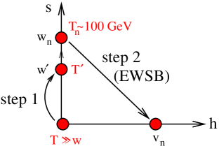
Figure 1: Sequence of phase transitions in field space.

III Phase Transition

Because of our assumption that $\langle s\rangle=0$ at low temperatures, the $\lambda_{hs}h^{2}s^{2}$ coupling creates a barrier in field space between the false and true vacua, and gives rise to a two-step phase transition. At temperatures $T\gg w$, the minimum of the potential is at the origin, where both electroweak symmetry and the $Z_{2}$ symmetry are restored. At some temperature $T^{\prime}$, the first transition occurs, where $\langle s\rangle\to w^{\prime}$ (see fig. 1). As $T$ decreases, $\langle s\rangle$ and the corresponding minimum of the potential becomes metastable. At the critical temperature $T_{c}$, the two minima become degenerate, and at a slightly lower temperature $T_{n}$ nucleation of bubbles begins, signaling the second transition where electroweak symmetry is broken while the $Z_{2}$ symmetry is restored. These two transitions are summarized as

1. At $T=T^{\prime}$ $(h,s):(0,0)\rightarrow(0,w^{\prime})$

2. At $T=T_{n}$ $(h,s):(0,w_{n})\rightarrow(v_{n},0)$ .

It is the second transition that is important for baryogenesis. We note that while domain walls could form during the first transition, the restoration of the $Z_{2}$ symmetry during the second transition will cause them to annihilate. This occurs long before they can dominate the energy density of the universe, hence we expect that no cosmological problems will arise from this brief appearance of domain walls Espinosa:2011eu .

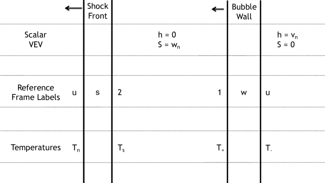
Figure 2: Illustration of the geometry of a deflagration. The bubble wall and shock front are moving to the left with the inside of the bubble being on the right of the figure.

The dynamics of the phase transition depend strongly on $T_{n}$, the temperature at which the probability of a bubble nucleating within one Hubble volume per Hubble time is $\mathcal{O}(1)$ Quiros:1999jp . The tunneling probability goes as $\exp(-S_{3}/T)$, where $S_{3}$ is the three-dimensional Euclidean action. We used CosmoTransitions Wainwright:2011kj to find phase transition candidates and to determine $T_{n}$. The criterion for the nucleation temperature is taken to be $S_{3}/T_{n}=140$ Quiros:1999jp .

Since our investigation is motivated by electroweak baryogenesis, we focus attention on first order transitions that are strong enough to preserve the baryon asymmetry from washout by residual sphaleron interaction inside the bubbles. This requires the Higgs VEV at the nucleation temperature to satisfy Moore:1998swa

$${v_{n}\over T_{n}}\gtrsim 1.1\,.$$ (5)

IV Wall Dynamics

The bubble-wall dynamics are determined by the interactions of the Higgs and singlet fields with a thermal fluid consisting of top quarks, electroweak gauge bosons, and any other particles to which the scalars couple significantly. After the bubble nucleates, it expands due to the outward pressure caused by the potential difference between the phases of the scalar fields on either side. The interactions of the wall with the surrounding fluid counteract the expansion by a friction force that depends on the speed and shape of the wall.

If the friction is strong enough, the bubbles reach a steady-state velocity whose value is relevant for gravitational waves and baryogenesis. The terminal $v_{w}$ depends upon the field profiles that solve the equations of motion. These in turn depend upon the temperature $T_{w}$ of the wall and the $v_{w}$-dependent friction exerted by the plasma on the wall, leading to $T_{w}>T_{n}$, due to heating by the fluid. A self-consistent solution thus requires simultaneously solving for $v_{w}$ and the scalar field profiles in the wall.

IV.1 Deflagration profiles

The wall temperature, and the rest of the dynamics of the bubble, depend on whether the phase transition proceeds through deflagrations or detonations (hybrids of these two are also possible). For subsonic bubble walls, with $v_{w}<1/\sqrt{3}$, the bubbles grow via deflagrations Espinosa:2010hh , in which the wall is preceded by a shock front that moves through the fluid, perturbing it, increasing the temperature from $T_{n}$ to $T_{s}$ and causing the wall to move (see fig. 2). The fluid velocity decreases until the point where the wall passes it, so that the fluid behind the wall is at rest relative to that preceding the shock front. In this work we limit our investigation to the case of deflagrations, hence subsonic walls, deferring the study of supersonic walls to the future WIP .

Because of the heating, the bubble wall dynamics are not determined at temperature $T_{n}$, but rather the temperature of the fluid near the wall. The calculation is performed at times sufficiently long after nucleation that the bubble has reached a steady-state velocity, and the profiles of the fluid perturbations vary on scales much larger than the wall thickness. Therefore one approximates the wall as a discontinuity, such that the fluid temperature is $T_{+}$ ($T_{-}$) just in front of (behind) the wall. The fluid velocity likewise is discontinuous there.

Since it is often convenient to switch between reference frames, we adopt the notation $v_{xy}$ for the velocity of $x$ in the reference frame $y$. In this context, $x$ and $y$ either refer to the wall ($w$), shock front ($s$), or the fluid at position $1$ (in front of the wall), $2$ (behind the shock front), or $u$ (the unperturbed “universe” frame, in front of the shock front or behind the wall). The wall velocity, which is measured with respect to the fluid directly in front of the wall, is $v_{w1}$ in this notation. We note that for any $x$ and $y$, $v_{xy}=-v_{yx}$. A diagram depicting the geometry and labels is shown in fig. 2.

The relationships between the various fluid velocities and temperatures are found by integrating the stress tensor $T_{\mu\nu}$ across either of the two interfaces shown in fig. 2. Approximating the fluid as perfect, these depend only on the fluid density and pressure. The equations of state can be expressed as Kozaczuk:2015owa

$$p_{\pm}=\frac{1}{3}a_{\pm}(T_{n})T_{\pm}^{4}-\epsilon_{\pm}(T_{n})$$ (6)

$$\rho_{\pm}=a_{\pm}(T_{n})T_{\pm}^{4}+\epsilon_{\pm}(T_{n})$$ (7)

where $\rho_{\pm}$ is the fluid density on either side of the bubble wall and $p_{\pm}$ is the pressure. $a_{\pm}$ and $\epsilon_{\pm}$ are given by

$$a_{\pm}(T)=-\frac{3}{4T^{3}}\,\frac{d\mathcal{F}_{\pm}(T)}{dT}$$ (8)

$$\epsilon_{\pm}(T)=\mathcal{F}_{\pm}(T)+\frac{1}{3}a_{\pm}(T)T^{4}\,.$$ (9)

$\mathcal{F}_{\pm}$ is the free energy of the fluid evaluated at the respective VEVs outside and inside wall and $T=T_{n}$. It is given by

$$\mathcal{F}(h,s,T)=V_{\rm eff}(h,s,T)-\frac{g_{*}^{\prime}\,\pi^{2}}{90}T^{4}\,.$$ (10)

Here $g_{*}^{\prime}=107.75-24.5=83.25$ is the effective number of degrees of freedom, apart from the $t$, $W/Z$, $h$, $\chi$ and $s$, whose contributions are already included in $V_{\rm eff}$. In general, $a_{\pm}(T)$ and $\epsilon_{\pm}(T)$ in (6,7) should be evaluated at the temperatures $T_{\pm}$, but for transitions typically of interest for baryogenesis, where there is a limited degree of supercooling, the $T$-dependence of $a(T)$ and $\epsilon(T)$ is insignificant.

Integrating $T_{\mu\nu}$ across the bubble wall provides the relations Espinosa:2010hh

$$v_{w1}v_{wu}=\frac{p_{+}-p_{-}}{\rho_{+}-\rho_{-}},\quad\frac{v_{w1}}{v_{wu}}=\frac{p_{+}+\rho_{-}}{\rho_{+}+p_{-}}\,.$$ (11)

Integrating across the shock front, the temperature changes, but not the the field values, leading to

$$v_{su}v_{s2}=\frac{1}{3},\quad\frac{v_{su}}{v_{s2}}=\frac{T_{n}^{4}+3T_{s}^{4}}{3T_{n}^{4}+T_{s}^{4}}\,.$$ (12)

Fluid velocities in the wall and shock wave frame are related by Lorentz transforming to the $u$ frame using

$$v_{2u}=\frac{v_{su}-v_{s2}}{1-v_{su}v_{s2}},\quad v_{1u}=\frac{v_{wu}-v_{w1}}{1-{v_{wu}v_{w1}}}\,.$$ (13)

The relationship between the fluid velocity and temperature behind the shock front and in front of the wall can be approximated by linearizing the stress-energy equations with respect to small fluid velocities in the universe frame Huber:2013kj , to obtain

$$T_{s}=T_{+}\exp\bigg{[}\frac{-2v_{u1}v_{wu}^{2}}{1-3v_{wu}^{2}}\bigg{(}\frac{1}{v_{wu}}-\frac{1}{v_{su}}\bigg{)}\bigg{]}$$ (14)

$$v_{2u}=v_{1u}\bigg{(}\frac{v_{wu}}{v_{su}}\bigg{)}^{2}\bigg{(}\frac{3v_{su}^{2}-1}{3v_{wu}^{2}-1}\bigg{)}$$ (15)

For a given guess of the wall velocity, $v_{w}\equiv v_{w1}$, and an associated nucleation temperature, eqs. (11-15) can be used to solve for the eight remaining variables: $T_{+}$, $T_{-}$, $T_{s}$, $v_{wu}$, $v_{su}$, $v_{1u}$, $v_{2u}$, and $v_{s2}$. An example of the solution to these equations for sample set of parameters is shown in fig. 3.

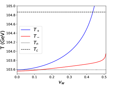
Figure 3: An example of how the wall temperature changes as a function of $v_{w}$ for a sample model with $m_{s}=63\textrm{ GeV}$, $w_{0}=130\textrm{ GeV}$, and $\lambda_{hs}=0.9$

IV.2 Equations of Motion

The equation of motion of a scalar field coupled to a perfect fluid has been derived by enforcing the conservation of the stress-energy tensor in the WKB approximation Moore:1995si , or starting from the Kadanoff-Baym equations Konstandin:2014zta . Both methods lead to

$$\Box\phi+\frac{\partial V(\phi)}{d\phi}+\sum_{i}n_{i}\frac{dm_{i}^{2}}{d\phi}\int\frac{d^{3}p}{(2\pi)^{3}2E}\,f_{i}(\vec{p},x)=0$$ (16)

where $V(\phi)$ is the zero-temperature effective potential, the sum is over all particles that couple to $\phi$, $n_{i}$ is the number of degrees of freedom of particle $i$, $m_{i}$ is its field-dependent mass, and $f_{i}(\vec{p},x)$ is its phase space distribution. By separating $f_{i}=f_{0,i}+\delta\!f_{i}$ into equilibrium and out-of-equilibrium components, the equation of motion takes a more useful form. The integral over $f_{0,i}$ is equivalent to accounting for the $T$-dependence of the effective potential, giving

$$\Box\phi+\frac{\partial V_{\rm eff}(\phi,T)}{d\phi}+\sum_{i}n_{i}\frac{dm_{i}^{2}}{d\phi}\!\!\int\!\!\frac{d^{3}p}{(2\pi)^{3}2E}\,\delta\!f_{i}(\vec{p},x)=0$$ (17)

The third term in (17) describes the friction force that comes from the dissipative interactions between the scalar field and the surrounding fluid.

In the following, we assume that the dominant sources of friction are the top quark and electroweak gauge bosons. The lighter fermions, gluons and photons can be safely ignored because of their negligible couplings to the Higgs field. The self-couplings and mixing of the scalar fields are assumed to be subdominant due to their fewer degrees of freedom relative to vector bosons or quarks. It is possible that including these contributions would lead to moderately slower walls, which could be advantageous for baryogenesis, but we defer this issue to future study.

For the electroweak phase transition considered here, there are two relevant scalar fields, each with its own equation of motion, that must be simultaneously solved. Eq. (17) can be further simplified by accounting for the spherical symmetry of the wall and going to the planar limit, which reduces the system to one spatial dimension, and by considering only the steady-state regime. Therefore, the equations of motion for a bubble wall traveling in the negative $z$ direction become

$$-h^{\prime\prime}(z) + \frac{\partial V_{\rm eff}(h,s,T)}{\partial h}$$

$$+ \sum_{i=t,W,Z}n_{i}\frac{dm_{i}^{2}}{dh}\int\frac{d^{3}p}{(2\pi)^{3}2E}\,\delta\!f_{i}(\vec{p},z)=0$$

$$-s^{\prime\prime}(z) + \frac{\partial V_{\rm eff}(h,s,T)}{\partial s}=0$$ (19)

where primes denote derivatives with respect to $z$. Strictly speaking, the existence of a steady-state solution to the equations of motion does not guarantee that those solutions will in fact be realized in the physical setting, but this issue is beyond the scope of this paper.

IV.3 Friction

The friction experienced by the wall depends on $\delta\!f_{i}(\vec{p},z)$, the deviation from equilibrium of $W/Z$ and $t$. We adopt the fluid approximation framework developed in Moore:1995si , in which the friction is fully described by three fluids: that of the top quark, the massive gauge bosons, and the other particles, denoted as the “background.”   We label the gauge boson contribution by $W$ although it also includes $Z$. For simplicity $W$ and $Z$ are grouped together due to their similar couplings, and assigned a mass-squared that is the weighted average of $m_{W}^{2}$ and $m_{Z}^{2}$. The background fluid encompasses all the fields that are assumed to contribute negligible friction, but which nevertheless play an important role in the wall dynamics. We consider friction only from fluid excitations with large momentum, such that the wavelength is shorter than the width of the wall. It has been shown that IR excitations in the massive gauge boson fluid can be important Moore:2000wx , but we have checked numerically that these are subdominant for parameters of interest in the present study, using the same approximations to evaluate the IR contributions as in ref. Kozaczuk:2015owa , but taking care to impose the perturbative cutoff $m_{W}(z)>g^{2}T$ Moore:2000wx .

The phase space distribution for the $t$ and $W$ fluids can be parametrized as

$$f_{i}(E,z)=\frac{1}{e^{(E+\delta_{i}(z))/T}\pm 1}$$ (20)

where the $+/-$ is for fermions/bosons and

$$\delta_{i}(z) = -\Big{[}T(\delta\mu_{i}+\delta\mu_{bg})(z)+E(\delta\tau_{i}+\delta\tau_{bg})(z)$$ (21)

$$+ p_{z}(\delta v_{i}+\delta v_{bg})(z)\Big{]}$$

accounts for perturbations in the fluids. $\delta\mu_{i}(z)$, $\delta\tau_{i}(z)$, $\delta v_{i}(z)$ are respectively the perturbations in the chemical potential, the relative temperature and the velocity. The subscript $bg$ denotes the background fluid. All the perturbations are relative to the fluid directly in front of the wall where $\mu=0$ and $T=T_{+}$ as described in section IV.1.

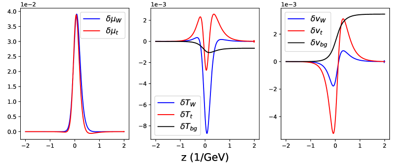
Figure 4: Example of the solutions for the fluid perturbations, for a model with $m_{s}=63\textrm{ GeV}$, $w_{0}=130\textrm{ GeV}$, and $\lambda_{hs}=0.9$, $v_{w}=0.128$ and background wall shape $h(z)=({h_{0}}/{2})[\tanh({z}/{L_{w}})+1]$ where $h_{0}=209\textrm{ GeV}$ and $L_{w}=0.2\textrm{ GeV}^{-1}$.

Deviations from equilibrium in the fluids are governed by the Boltzmann equation

$${d\over dt}f_{i}(E,z)=-C[f_{i}(E,z)]\,.$$ (22)

Rather than solving the full Boltzmann equation, one linearizes it in $\delta_{i}(z)$, and converts it to a system of ordinary differential equations by taking three moments: $\int{d^{\,3}p}/{(2\pi)^{3}}$, $\int(E/T)\,{d^{\,3}p}/(2\pi)^{3}$, and $\int{p_{z}\,d^{\,3}p}/{(2\pi)^{3}}$. A detailed derivation is provided in appendix B, leading to the coupled matrix equations

$$A_{\scriptscriptstyle W}(\vec{q}_{\scriptscriptstyle W}+\vec{q}_{bg})^{\prime}+\Gamma_{\scriptscriptstyle W}\vec{q}_{\scriptscriptstyle W} = S_{\scriptscriptstyle W}$$ (23)

$$A_{t}(\vec{q}_{t}+\vec{q}_{bg})^{\prime}+\Gamma_{t}\vec{q}_{t} = S_{t}$$ (24)

$$A_{bg}\vec{q}^{\,\prime}_{bg}+\Gamma_{bg,{\scriptscriptstyle W}}\vec{q}_{\scriptscriptstyle W}+\Gamma_{bg,t}\vec{q}_{t} = 0$$ (25)

where $\vec{q}_{i}^{\textrm{ }T}=~{}(\delta\mu_{i},\delta\tau_{i},\delta v_{i})$. The $A_{i}$ matrices for $i=W,t$ take the form

$$A_{i}\equiv\begin{bmatrix}v_{w}c_{2}^{i}&v_{w}c_{3}^{i}&\frac{1}{3}d_{3}^{i}\\ v_{w}c_{3}^{i}&v_{w}c_{4}^{i}&\frac{1}{3}d_{4}^{i}\\ \frac{1}{3}d_{3}^{i}&\frac{1}{3}d_{4}^{i}&\frac{1}{3}v_{w}d_{4}^{i}\end{bmatrix}$$ (26)

while the source terms are

$$S_{i}\equiv\frac{m_{i}^{\prime}m_{i}^{\phantom{{}^{\prime}}}}{T^{2}}\begin{bmatrix}v_{w}c_{1}^{i}\\ v_{w}c_{2}^{i}\\ 0\end{bmatrix}$$ (27)

The coefficients $c_{j}^{i}$ and $d_{j}^{i}$ denote the integrals

$$c_{j}^{i}\left(\frac{m_{i}}{T}\right)\equiv\int\frac{d^{3}{p}}{(2\pi)^{3}}\big{(}-f_{0,i}^{\prime}\big{)}\frac{E^{j-2}}{T^{j+1}}$$ (28)

and

$$d_{j}^{i}\left(\frac{m_{i}}{T}\right)\equiv\int\frac{d^{3}{p}}{(2\pi)^{3}}\big{(}-f_{0,i}^{\prime}\big{)}\frac{p^{2}E^{j-4}}{T^{j+1}}$$ (29)

where $f_{0,i}$ is the equilibrium distribution function for particle $i$. In previous literature (with the exception of ref. Laurent:2020gpg ), these coefficients were evaluated in the massless approximation, where $d_{j}^{i}=c_{j}^{i}$, setting $m_{i}/T=0$. But for some phase transitions satisfying the sphaleron bound (5), $m_{t}/T>1$ in the broken phase; hence we we derived the full mass dependence for this work. For the background fluid, one can show that

$$A_{bg}=20A_{\scriptscriptstyle W}|_{m=0}+78A_{t}|_{m=0}$$ (30)

where the background fluids are approximated as massless Konstandin:2014zta .

IV.3.1 Collision terms

The $\Gamma_{i}$ matrices in eqs. (23, 24) quantify the interactions of the fluids. $\Gamma_{t}$ and $\Gamma_{\scriptscriptstyle W}$ take the form

$$\Gamma_{i}\equiv T\begin{bmatrix}\Gamma_{\mu 1i}&\Gamma_{\delta T1i}&0\\ \Gamma_{\mu 2i}&\Gamma_{\delta T2i}&0\\ 0&0&\Gamma_{vi}\,.\end{bmatrix}$$ (31)

The matrix elements were originally computed in ref. Moore:1995si , to leading-log accuracy in the masses of particles exchanged in the various interactions. This means that the infrared divergence that would arise from $t$-channel exchange of massless particles (in the electroweak symmetric phase) is cut off by taking account of their thermal masses in the propagator, while neglecting such mass effects otherwise. Several calculational errors in Moore:1995si were subsequently corrected in Ref. Arnold:2000dr , which we take into account here.

In ref. Kozaczuk:2015owa , a refined leading log calculation was carried out, including hard thermal loops, for the top quark and Higgs scattering rates, but not for $W$ bosons, since it was argued there that the $W$ contribution to friction could be determined from IR-dominated modes described by treating the $W$ as a classical field Moore:2000mx . We have found that these contributions are numerically smaller in the present model than the perturbative ones from the original calculation Moore:1995si , so this approach would not be consistent here. Moreover the inclusion of extra annihilation channels like $t\bar{t}\to hh$, carried out in Kozaczuk:2015owa , would not be consistent in our present approach, where we approximate the Higgs fluid as maintaining thermal equilibrium, by omitting its perturbations from the Boltzmann network.

Instead, we have improved on the original estimates of Moore:2000mx using results from ref. Laurent:2020gpg , which recomputed the phase space integrals numerically instead of approximating them analytically, leading to

$$\Gamma_{\scriptscriptstyle W}/T = \begin{bmatrix}0.00239&0.00512&0\\ 0.00512&0.0174&0\\ 0&0&0.00663\end{bmatrix}$$

$$\Gamma_{t}/T = \begin{bmatrix}0.00196&0.00445&0\\ \ 0.00445&0.0177&0\\ 0&0&0.00992\end{bmatrix}$$ (32)

The effect of using this collision term compared to that of Moore:1995si , is explored in section V.1.

Using energy-momentum conservation, the background fluid collision terms are given by

$$\Gamma_{bg,i}=-n_{i}\Gamma_{i}$$ (33)

where $n_{t}=12$ and $n_{W}=9$ are the number of degrees of freedom in the respective components.

The background fluid is assumed to be in chemical equilibrium, implying that $\delta\mu_{\rm bg}=0$. This assumption removes the top row of eq. (25). The remaining two rows determine $\delta\tau_{\rm bg}$ and $\delta v_{\rm bg}$ in terms of $q_{\scriptscriptstyle W}$ and $q_{t}$,

$$\vec{q}_{\textrm{bg}}^{\textrm{ }\prime}=-A_{bg23}^{-1}(\Gamma_{\textrm{bg},{\scriptscriptstyle W}}\vec{q}_{\scriptscriptstyle W}+\Gamma_{\textrm{bg},t}\vec{q}_{t})$$ (34)

where $A_{bg23}^{-1}$ denotes the matrix where the bottom right block of $A_{bg}$ is inverted and the rest of the matrix elements are zero.

Equations (23) and (24) can then be expressed in $6\times 6$ matrix form, in the rest frame of the bubble wall,

$$A\vec{q}^{\textrm{ }\prime}+\Gamma\vec{q}=S$$ (35)

with

$$A \equiv \gamma\begin{bmatrix}A_{W}&0\\ 0&A_{t}\end{bmatrix},\ \vec{q}\equiv\begin{bmatrix}\vec{q}_{\scriptscriptstyle W}\\ \vec{q}_{t}\end{bmatrix},\ S\equiv\gamma\begin{bmatrix}S_{\scriptscriptstyle W}\\ S_{t}\end{bmatrix}$$ (36)

and

$$\Gamma\equiv\begin{bmatrix}\Gamma_{\scriptscriptstyle W}&0\\ 0&\Gamma_{t}\end{bmatrix}-\begin{bmatrix}A_{\scriptscriptstyle W}A_{\textrm{bg}23}^{-1}\Gamma_{\textrm{bg},{\scriptscriptstyle W}}&A_{\scriptscriptstyle W}A_{\textrm{bg}23}^{-1}\Gamma_{\textrm{bg},t}\\ A_{t}A_{\textrm{bg}23}^{-1}\Gamma_{\textrm{bg},{\scriptscriptstyle W}}&A_{t}A_{\textrm{bg}23}^{-1}\Gamma_{\textrm{bg},t}\end{bmatrix}$$ (37)

The factors of $\gamma=1/\sqrt{1-v_{w}^{2}}$ are from Lorentz boosting to the rest frame of the wall.

The $W$ and $t$ fluid perturbations are determined by solving eq. (35) using the relaxation method as described in ref. Press:1992 , since shooting tends to be unstable. The background fluid perturbations are found by integrating eq. (34). One can carry out this procedure for given values of the wall velocity and shape, and from the ensuing perturbations compute the friction term in the Higgs field equation of motion (IV.2) using

$$\int\frac{d^{3}p}{(2\pi)^{3}2E}\,\delta\!f_{i}(\vec{p},z) \cong \int\frac{d^{3}p}{(2\pi)^{3}2E}f_{0,i}^{\prime}(\vec{p},z)\,\delta_{i}(z)$$

$$=\frac{T^{2}}{2}\Big{[}c_{1}^{i}(z)\delta\mu_{i}(z) + c_{2}^{i}(z)\big{(}\delta\tau_{i}(z)+\delta\tau_{bg}(z)\big{)}\Big{]}$$

An example of the solutions for the perturbations is shown in fig. 4.

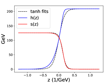
Figure 5: The wall shape that solves the equation of motion for the model with $m_{s}=63\textrm{ GeV}$, $w_{0}=130\textrm{ GeV}$, and $\lambda_{hs}=0.9$. The dashed curves show the best fits using the tanh ansatz of eqs. (48 , 49).

IV.4 Solving the Equations of Motion

With the friction calculated in eq. (IV.3.1), the equations of motion that must be solved to determine $v_{w}$ and the shape of the wall are

$$-h^{\prime\prime}(z) + \frac{\partial V_{\textrm{eff}}(h,s,T_{+})}{\partial h}$$

$$+ \frac{n_{t}T_{+}}{2}\frac{dm_{t}^{2}}{dh}\left[c_{1}^{t}\delta\mu_{t}+c_{2}^{t}(\delta\tau_{t}+\delta\tau_{bg})\right]$$

$$+ \frac{n_{W}T_{+}}{2}\frac{dm_{W}^{2}}{dh}\left[c_{1}^{W}\delta\mu_{W}+c_{2}^{W}(\delta\tau_{W}+\delta\tau_{bg})\right]=0$$

$$-s^{\prime\prime}(z) + \frac{\partial V_{\textrm{eff}}(h,s,T_{+})}{\partial s}=0\,.$$ (40)

Deep into the bubble interior, eq. (IV.4) is not exactly satisfied once we adopt our approximation schemes for calculating the effective potential and the perturbations. The Higgs’ VEV is unchanging there, so the kinetic term is zero. Similarly the perturbations in the $W$ and $t$ fluids go to zero on both sides of the wall. This implies that the terms proportional to $\delta\tau_{bg}$ must exactly cancel out the potential term. When the perturbations are determined as described above and the potential term is calculated with the Higgs VEV that minimizes the potential inside the bubble, the two terms do not cancel as they should. This is due to differences in the derivation of the friction terms in comparison to the effective potential. Firstly, the fluid perturbations are only determined to linear order whereas the temperatures that go into the effective potential, $T_{+}$ and $T_{-}$, were calculated including non-linearities in the fluid equations. This means that while in theory $T_{+}-T_{-}=T_{+}\delta\tau_{bg}$, their relationship is only approximate. The other cause is that the scalar fields were treated as massless background fields in the friction calculation but their full contribution was included in the effective potential. There are three ways to account for this inconsistency: the Higgs VEV inside the bubble can be chosen not to minimize the potential but instead to cancel the friction term, the entire friction can be scaled to cancel the potential term but maintaining the friction shape in $z$, or just the background perturbation contribution to the friction can be scaled to cancel the potential term. We adopt the last option, which we found to be the most conservative choice (leading to slightly larger wall velocities). The equations of motion that we actually use to determine the wall dynamics then become

$$E_{h} \equiv -h^{\prime\prime}(z)+\frac{\partial V_{\textrm{eff}}(h,s,T_{+})}{\partial h}$$

$$+ \frac{n_{t}T_{+}}{2}\frac{dm_{t}^{2}}{dh}\left[c_{1}^{t}\delta\mu_{t}+c_{2}^{t}(\delta\tau_{t}+y\delta\tau_{bg})\right]$$

$$+ \frac{n_{W}T_{+}}{2}\frac{dm_{W}^{2}}{dh}\left[c_{1}^{W}\delta\mu_{W}+c_{2}^{W}(\delta\tau_{W}+y\delta\tau_{bg})\right]=0$$

$$E_{s} \equiv -s^{\prime\prime}(z)+\frac{\partial V_{\textrm{eff}}(h,s,T_{+})}{\partial s}=0\,$$ (42)

where $y$ is an $\mathcal{O}(1)$ parameter chosen so that the equations are satisfied for larger positive values of $z$.

For a given value of $v_{w}$, the relaxation method can be used to find the shapes of $h(z)$ and $s(z)$ that come closest to solving the equations of motion. One must then vary $v_{w}$ and find a complete solution to the equations, by iterating this procedure. A reasonable initial guess for both $v_{w}$ and the wall shape is required, leading us to solve the equations in two stages. The first part is to guess $v_{w}$ and the wall shape using the $\tanh$ ansatz employed in previous studies of wall velocities Moore:1995si ,Konstandin:2014zta ,Kozaczuk:2015owa . The second uses these as a starting point to numerically determine $v_{w}$ and the wall shapes.

The $\tanh$ ansatz in the first stage assumes that the Higgs profile has the form

$$h(z)=\frac{v(T_{-})}{2}\left(\tanh\left(\frac{z}{L_{w}}\right)+1\right)$$ (43)

where $v(T_{-})$ is the Higgs VEV at temperature $T_{-}$ and $L_{w}$ is the width of the wall. The friction and shape of the singlet profile are independent of each other, so there is no need to impose a $\tanh$ ansatz for $s$; rather its profile is found by numerically solving its equation of motion. This reduces the problem to finding values of $v_{w}$ and $L_{w}$ that come closest to solving the Higgs equation of motion.

No choice of $v_{w}$ and $L_{w}$ will exactly solve eq. (IV.4), since the true shape is not a $\tanh$ function. Instead we follow ref. Konstandin:2014zta by calculating two moments of $E_{h}$ in eq. (IV.4) and finding the values of $v_{w}$ and $L_{w}$ that make them vanish. The two moments are taken to be

$$E_{1} \equiv \int h^{\prime}(z)\,E_{h}\,dz=0$$ (44)

$$E_{2} \equiv \int h^{\prime}(z)\big{(}2h(z)-v(T_{-})\big{)}\,E_{h}\,dz=0$$

since with this choice the Jacobian matrix $\partial(E_{1},E_{2})/\partial(v_{w},L_{w})$ is always far from being singular.

The first stage of the algorithm can then be summarized as:

1. Make a guess for $v_{w}$ and $L_{w}$

2. Calculate $T_{+}$ and $T_{-}$ for $v_{w}$

3. Determine $s(z)$ by solving the $s$ equation of motion using the $\tanh$ ansatz for $h(z)$

4. Determine the shape of the friction term for the guessed shape of $h(z)$

5. Calculate the moments $E_{1}$ and $E_{2}$

6. Find the new guess for $v_{w}$ and $L_{w}$ by solving $E_{i}=0$.

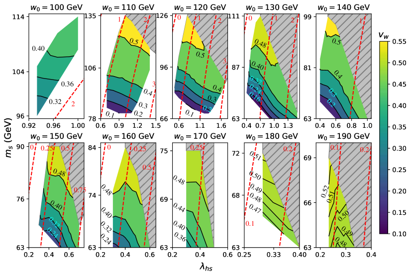
Figure 6: Contours of the wall velocity $v_{w}$ in the $\lambda_{hs}$-$m_{s}$ plane, with $w_{0}$ increasing from 100 to 190 GeV in successive plots. The white area indicates regions where no first order transition satisfying the sphaleron bound (5) was found. In the grey hatched region, strong transitions satisfying (5) exist, but no solutions with $v_{w}<c_{s}$ were found. The red dashed contours indicate values of the singlet self-coupling, $\lambda_{s}$, as determined by eq. (2). For each $w_{0}$ we show only regions containing viable solutions for the bubble wall parameters, within the ranges specified in Eqn. (V).

In the second stage, we aimed to relax the $\tanh$ profile assumption for $h(z)$ and to determine its shape more exactly. Using the values of $v_{w}$ and $L_{w}$ from the first part as new initial guesses, we solved both $h$ and $s$ equations of motion simultaneously, using relaxation. A challenge here is that the friction on the wall, which is expensive to compute, depends on the background $h(z)$ solution. To speed up the algorithm, we recomputed the friction only after several relaxation steps. This procedure leads to eventual convergence, unless the initial guess for $v_{w}$ is too poor. Convergence was tested by seeing how closely the two equations of motion were satisfied, using the squared error statistic

$$E_{\rm tot}=\int\left[E_{h}^{2}+E_{s}^{2}\right]dz\,.$$ (45)

The best value of $v_{w}$ was determined by varying $v_{w}$ in the region of the guess from step 1 as to minimize $E_{\rm tot}$. An example of the wall shapes that solve the equations of motion is given in fig. 5. It demonstrates that the actual profiles can differ significantly from the tanh ansatz.

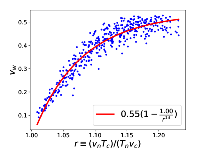
Figure 7: The dependence of wall velocity, $v_{w}$, on the supercooling parameter, $r=(v_{n}/T_{n})/(v_{c}/T_{c})$. The solid curve shows a fit to the points.

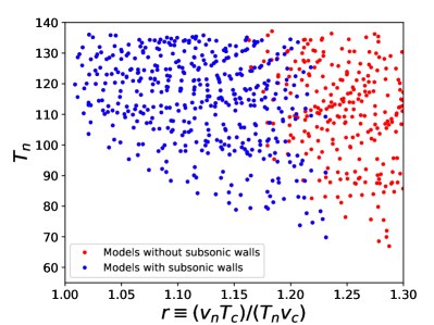
Figure 8: Scatter plot of nucleation temperature $T_{n}$ versus the supercooling parameter $r$, for all models CosmoTransitions found to satisfy the sphaleron washout condition.

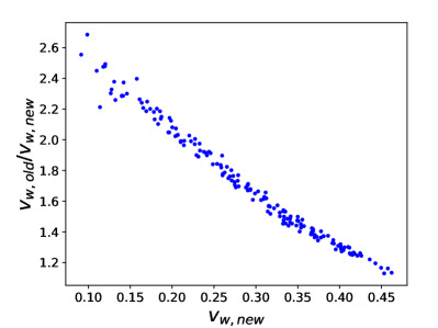
Figure 9: Comparison of wall velocities determined using the corrected interaction rates in eq. (IV.3.1) ($v_{w,new}$) compared to the incorrect wall velocities that would be found by using the interaction rates reported in Moore:1995si ($v_{w,old}$).

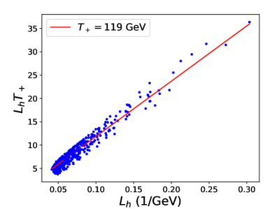
Figure 10: The Higgs wall width $L_{h}$, in units of the inverse wall temperature $T_{+}^{-1}$, versus the same quantity in GeV^-1 units. The solid line shows a fit to the points, corresponding to the mean wall temperature $T_{+}=119$ GeV.

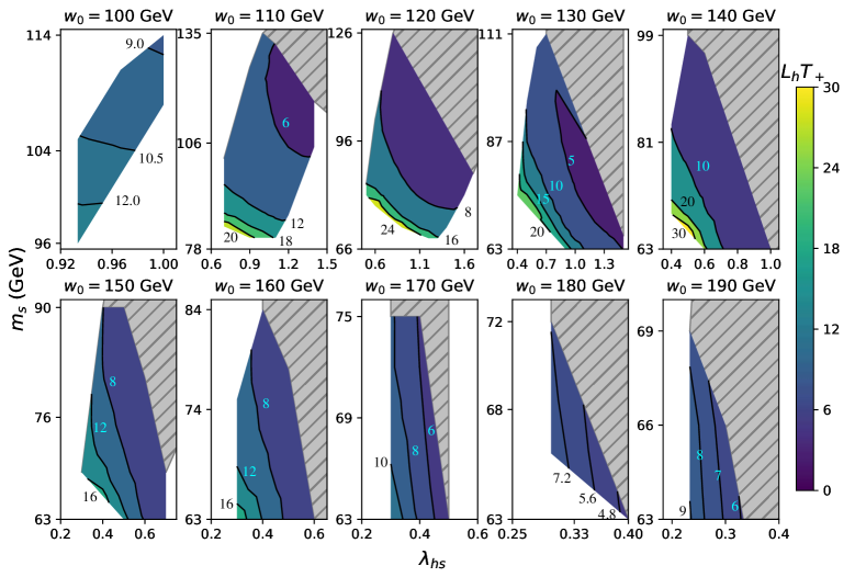
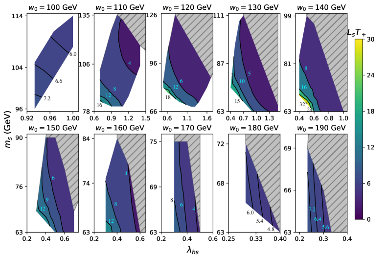
Figure 11: Top two rows (a): Like fig. 6, but showing the contours of the Higgs wall width $L_{h}T_{+}$ where $T_{+}$ is the temperature in front of the bubble wall. Bottom two rows (b): Like fig. 6, but showing the contours of the singlet wall width $L_{s}T_{+}$.

(a)

(b)

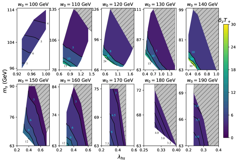
Figure 12: Like fig. 6, but showing the contours of the wall separation parameter $\delta_{z}$, defined in eq. (49).

V Results and Discussion

A scan of the parameter space of the scalar singlet model was performed in the ranges

$$0.1 \leq \lambda_{hs}\leq 1.8$$

$$63\,\textrm{GeV} \leq m_{s}\leq 138\,\textrm{GeV},$$ (46)

$$100\,\textrm{GeV} \leq w_{0}\leq 190\,\textrm{GeV}.$$

We did not find viable examples for $w_{0}\lesssim 90\,$GeV and only a single point in parameter space that produces subsonic walls for $w_{0}\gtrsim 200\,$GeV. Our results indicate that this covers most of the parameter space of interest for subsonic walls.

We imposed the lower bound $m_{s}>m_{h}/2$ so that collider constraints from invisible Higgs decay ($h~{}\to~{}ss$) do not apply Aaboud:2019rtt . This is a mild restriction, since for $m_{s}<m_{h}/2$ and not too close to the upper limit, these constraints imply the invisible branching ratio is $\lesssim 25\%$, hence $\lambda_{hs}\lesssim 0.01$, which is too small to give rise to a strong phase transition.

V.1 Wall Velocity Results

Our determinations of the wall speed over the full parameter space are illustrated in in fig. 6, showing contours of $v_{w}$ in the plane of $m_{s}$ versus $\lambda_{hs}$, for a series of $w_{0}$ values. The grey hatched regions indicate parameters for which no transitions with subsonic walls were found. One can see that models with heavier singlets and larger $\lambda_{hs}$ couplings tend to produce faster-moving walls. Generally we find a minimum value for $v_{w}$, which depends on $w_{0}$ and is smallest for $w_{0}\sim 120$ GeV, where the lowest speed $v_{w}\cong 0.1$ is found. The parameters specifying a few benchmark models and their resulting phase transition properties are shown in table 1.

$m_{s}$	$\lambda_{hs}$	$w_{0}$	$v_{w}$	$T_{n}$	$T_{c}$	$v_{n}/T_{n}$	$r$
63	0.9	130	0.128	103.592	104.865	2.02	1.02
81	1.0	110	0.142	124.301	125.425	1.40	1.03
66	0.3	160	0.306	130.532	132.677	1.28	1.05
105	0.8	110	0.426	130.646	134.461	1.24	1.11

Table 1: Benchmark models with successively faster moving walls. Masses and temperatures are in GeV. $r$ is the measure of supercooling defined in eq. (47).

Since it is numerically expensive to compute $v_{w}$ for a given model from first principles, it is useful to look for relations between it and other quantities characterizing the strength of the phase transition, that are easier to compute. In fact we observe a strong correlation between $v_{w}$ and the double ratio

$$r\equiv\frac{v_{n}/T_{n}}{v_{c}/T_{c}}$$ (47)

where $v/T$ is evaluated respectively at the nucleation and the critical temperatures. This is a measure of the degree of supercooling, and its correlation with $v_{w}$ is plotted in fig. 7, showing that $v_{w}$ increases rapidly with $r-1$. We find an analytic fit $v_{w}\cong 0.55\,(1-r^{-13})$, with deviations of order $\pm 0.03$. The maximum value of $r$ found for subsonic bubble walls was $r\cong 1.23$. It remains close to unity even for strong transitions, validating the assumption made in section IV.1 that the equations of state at the nucleation and critical temperatures do not differ significantly from each other.

The fact that a cutoff on $r$ exists, above which it is unlikely to produce subsonic walls, can be seen in fig. 8, which shows all the models tested, including those found not to have slow bubble walls. It clearly shows that for $r\gtrsim 1.25$, no transitions produce subsonic walls, whereas for $r\lesssim 1.15$ that all the models tested were found to do so.

The impact of the corrections made to the fluids’ collision term discussed in section IV.3.1 is shown in fig. 9. Using the collision term reported in Moore:1995si overestimates the wall velocities significantly. For the fastest walls that are subsonic in both calculations, the error is $\sim 20\%$, however, for the slowest walls using the incorrect collision term causes predictions of $v_{w}$ that is over double the true value. Additionally, since the corrected collision term predicts slower walls, a larger region of parameter space is found to produce subsonic walls than one would predict if using the incorrect collision term. This sensitivity to the collision term implies that further improvements to determining the fluid interaction rates is likely an important future step in improving the accuracy of the $v_{w}$ calculation.

Fig. 6 shows that subsonic walls require the singlet to be relatively light, $m_{s}\lesssim 135$  GeV, often with a relatively large coupling to the Higgs, $\lambda_{hs}\sim 1$. If $s$ is long-lived enough to escape detection within a collider, Refs. Craig:2014lda ; Ruhdorfer:2019utl ; Ramsey-Musolf:2019lsf suggest that a singlet with these properties may be a target at the high-luminosity LHC, or perhaps more realistically, at a future collider (from vector-boson fusion production of an off-shell Higgs). On the other hand, if we take the model at face value, as a complete model with a standard thermal history, Ref. Craig:2014lda also finds that the LUX direct detection experiment Akerib:2013tjd rules out $m_{s}\lesssim 120$ GeV even though $s$ would make a subdominant contribution to the dark matter. Of course, additional model ingredients can easily make $s$ unstable on cosmological time scales without affecting our phase-transition and wall-velocity results.

V.2 Wall Shape Results

Although Fig. 5 shows that the wall shapes deviate from a tanh profile, it is nevertheless a useful approximation for concisely encoding information about the wall shapes. We have accordingly analyzed our results from the fully numerical algorithm to find the best-fit tanh profiles, including a possible offset $\delta_{z}$ between the Higgs and the singlet profiles:

$$h_{\textrm{fit}} = \frac{h_{0}}{2}\bigg{[}1+\tanh\bigg{(}\frac{z}{L_{h}}\bigg{)}\bigg{]}$$ (48)

$$s_{\textrm{fit}} = \frac{s_{0}}{2}\bigg{[}1-\tanh\bigg{(}\frac{z-\delta_{z}}{L_{s}}\bigg{)}\bigg{]},$$ (49)

where we have allowed for independent widths $L_{h}$ and $L_{s}$ of the Higgs and singlet profiles.

To display results for the wall thicknesses, we have opted to use dimensionless combinations like $L_{h}T_{+}$, where $T_{+}$ is the temperature of the wall. If one wants to translate these into absolute thicknesses, it can be done using the strong correlation between $L_{h}T_{+}$ and $L_{h}$ in GeV^-1 units, shown in Fig. 10. Since all models with subsonic walls have nucleation temperatures in the range $70\,\textrm{GeV}\leq T_{n}\leq 140\,\textrm{GeV}$ (see Fig. 8), and for slow walls the wall temperature does not deviate much from the nucleation temperature, the relationship between these two ways of characterizing $L_{h}$ is linear with relatively little scatter: $L_{h}T_{+}\cong L_{h}\;119$ GeV. This reflects the fact that the deviations of wall temperature from the mean value $T_{+}=119\,$GeV are relatively small.

Contour plots of $L_{h}T_{+}$, $L_{s}T_{+}$, and $\delta_{z}T_{+}$ similar to those for $v_{w}$ are presented in Figs. 11 and 12. We find that faster walls tend to be thinner and have smaller offsets. These relationships are plotted in Figs. 13-15, which show strong correlations, especially in the case of $L_{h}$. With rare exceptions, $L_{s}<L_{h}$, with $L_{s}$ typically smaller than $L_{h}$ by 20-30%.

Figure 13: The dependence of Higgs wall width, $L_{h}$, on the wall velocity, $v_{w}$.

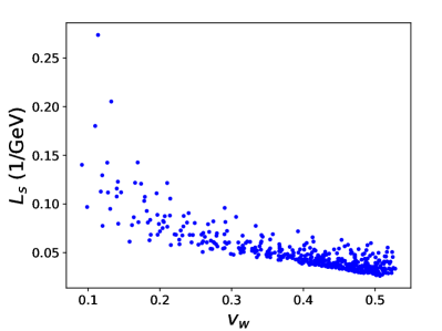
Figure 14: Like fig. 13 but for $L_{s}$.

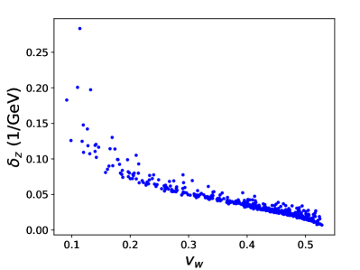
Figure 15: Like fig. 13 but for $\delta_{z}$.

VI Conclusion

This work has laid out a more quantitative methodology than has been previously used, for calculating the wall velocity of bubbles during the electroweak phase transition with an additional scalar field. We improved on previous similar studies by solving for the actual profiles of the scalar fields, rather than just parametrizing them using a $\tanh$ ansatz. Other improvements made here include use of the one-loop Coleman-Weinberg contributions to the potential including the effect of thermal masses, accounting for the sphericity of the bubbles, accounting for the $m/T$-dependence of the $A$-matrix coefficients of the fluid equations, and performing a scan over the three-dimensional parameter space.

Scanning over the parameter space reveals that the scalar singlet model is able to produce slow bubble walls that are preferable for electroweak baryogensis to occur, down to a minimum wall velocity of $v_{w}\cong 0.1$. These examples of slow-moving walls only occur in phase transitions with small amounts of supercooling.

There are several ways in which this study can be extended by future work. The precision of the wall velocity calculation could be improved by including additional sources of friction such as from the scalar fields and IR gauge boson modes. Moreover we have found that the results are rather sensitive to the collision rates $\Gamma_{i}$ that enter into the Boltzmann equations for the fluid perturbations. We have used leading-log results, that suffer from O(1) uncertainties. While this work was in progress, Ref. Wang:2020zlf presented new results for collision rates beyond the leading-log approximation, which in some cases exhibited surprisingly large differences from the leading-log counterparts.

For a complete analysis of electroweak baryogenesis in the $Z_{2}$ scalar singlet model, this analysis could be embedded in a more complete model that includes a new source of CP-violation in order to determine the size of the matter anti-matter asymmetry that would be produced. Lastly, extending this analysis to apply for faster walls or even supersonic walls could be of interest for studying other effects of the phase transition such as gravitational waves. We are currently studying these issues WIP .

Appendix A Effective potential

The one-loop contribution to the potential can be approximated as

$$V_{1}=\!\!\!\!\!\!\sum_{i={h,s,\chi,t,W,Z,\gamma}}\frac{n_{i}m_{i}^{4}(h,s,T)}{64\pi^{2}}\bigg{[}\textrm{ln}\bigg{(}\frac{m^{2}_{i}(h,s,T)}{v_{0}^{2}}\bigg{)}-c_{i}\bigg{]}$$ (50)

where $n_{i}$ is the number of degrees of freedom of each particle. For the scalar fields, longitudinal $W/Z$ and top quark $c_{i}=3/2$ but for the transverse gauge bosons $c_{i}=1/2$, in the $\overline{\hbox{MS}}$ scheme. The top quark is the only fermion included in the sum since the contributions from lighter fermions are suppressed by their small Yukawa couplings. $\chi$ stands for the Goldstone boson contributions.

The one-loop contribution acquires a temperature dependence through the thermal masses of the particles, in this method of carrying out the ring resummation Parwani:1991gq . It has been shown that for sufficiently strong phase transitions, a more careful treatment of thermal masses can be important Curtin:2016urg .

The scalar masses in eq. (50) are given by the eigenvalues of the mass matrix:

$$M^{2}_{\textrm{scalar},ij}\equiv\frac{\partial^{2}V}{\partial\phi_{i}\partial\phi_{j}}+m^{2}_{T,i}\delta_{ij}$$ (51)

where $\phi_{i}$ and $\phi_{j}$ are the five scalar fields summed over in eq. (50)and

$$m^{2}_{T,h} = T^{2}\left(\frac{3g^{2}+g^{\prime 2}}{16}+\frac{y_{t}^{2}}{4}+\frac{\lambda_{h}}{2}+\frac{\lambda_{hs}}{24}\right)$$ (52)

$$m^{2}_{T,\chi} = m^{2}_{T,h}$$ (53)

$$m^{2}_{T,s} = T^{2}\left(\frac{\lambda_{hs}}{6}+\frac{\lambda_{s}}{4}\right).$$ (54)

The three mass eigenvalues associated with the Goldstone bosons vanish in the vacuum state making those terms in eq. (50) formally divergent. This is properly dealt with by introducing a scale coinciding with the Higgs mass, $m_{h}$, to cut off the IR divergence Cline:1996mga .

The masses associated with the longitudinal modes of the gauge bosons in eq. (50) are given by the eigenvalues of the mass matrix:

$$M^{2}_{\textrm{long},ij} \equiv \begin{bmatrix}\frac{g^{2}h^{2}}{4}&0&0&0\\ 0&\frac{g^{2}h^{2}}{4}&0&0\\ 0&0&\frac{g^{2}h^{2}}{4}&\frac{gg^{\prime}h^{2}}{4}\\ 0&0&\frac{gg^{\prime}h^{2}}{4}&\frac{g^{\prime 2}h^{2}}{4}\\ \end{bmatrix}$$ (55)

$$+ \frac{11}{6}T^{2}\,\textrm{diag}(g^{2},g^{2},g^{2},g^{\prime 2})$$

The rest of the field-dependent masses in eq. (50) are given by:

$$m_{\textrm{trans},w}^{2} = \frac{g^{2}h^{2}}{4}$$

$$m_{\textrm{trans},z}^{2} = \frac{(g^{2}+g^{\prime 2})h^{2}}{4}$$

$$m_{\textrm{trans},\gamma}^{2} = 0$$

$$m_{t}^{2} = \frac{y_{t}^{2}h^{2}}{2}$$ (56)

The counterterm contribution to the potential can be parameterized as

$$V_{CT} = \frac{1}{2}\delta m_{h}^{2}h^{2}+\frac{1}{2}\delta m_{s}^{2}s^{2}+\frac{1}{4}\delta\lambda_{h}h^{4}+\frac{1}{4}\delta\lambda_{s}s^{4}$$ (57)

$$+ \frac{1}{4}\delta\lambda_{hs}h^{2}s^{2}$$

The five counterterms were chosen to ensure that the full effective potential at $T=0$ maintains its tree-level values for the scalar masses, potential minima, and scalar mixing. This is done by imposing the following conditions at $T=0$:

$$\frac{\partial V}{\partial h}\bigg{|}_{h=v_{0},s=0}=\ \ \ \frac{\partial V}{\partial s}\bigg{|}_{h=0,s=w_{0}}=0$$ (58)

$$\frac{\partial^{2}V}{\partial h^{2}}\bigg{|}_{h=v_{0},s=0}=m_{h}^{2},\quad\frac{\partial^{2}V}{\partial s^{2}}\bigg{|}_{h=v_{0},s=0}=m_{s}^{2}$$ (59)

and

$$\frac{\partial^{4}V}{\partial h^{2}\partial s^{2}}\bigg{|}_{h=v_{0},s=0}=\lambda_{hs}$$ (60)

where $m_{s}=\sqrt{\frac{1}{2}\lambda_{hs}v_{0}^{2}-\lambda_{s}w_{0}^{2}}$ is the mass of the scalar singlet in the true vacuum.

The resulting counterterm parameters are found to be

$$\delta m_{h}^{2}=\bigg{(}\frac{1}{2}\frac{\partial^{2}V_{1}}{\partial h^{2}}-\frac{3}{2v_{0}}\frac{\partial V_{1}}{\partial h}\bigg{)}\bigg{|}_{h=v_{0},s=0}$$ (61)

$$\delta m_{s}^{2}=\bigg{(}-\frac{\partial^{2}V_{1}}{\partial s^{2}}+\frac{v_{0}^{2}}{2}\frac{\partial^{4}V_{1}}{\partial h^{2}\partial s^{2}}\bigg{)}\bigg{|}_{h=v_{0},s=0}$$ (62)

$$\delta\lambda_{h}=\frac{1}{2v_{0}^{2}}\bigg{(}\frac{1}{v_{0}}\frac{\partial V_{1}}{\partial h}-\frac{\partial^{2}V_{1}}{\partial h^{2}}\bigg{)}\bigg{|}_{h=v_{0},s=0}$$ (63)

$$\delta\lambda_{s}=-\frac{\delta m_{s}^{2}}{w_{0}^{2}}-\frac{1}{w_{0}^{3}}\frac{\partial V_{1}}{\partial s}\bigg{|}_{h=0,s=w_{0}}$$ (64)

and

$$\delta\lambda_{hs}=-\frac{\partial^{4}V_{1}}{\partial h^{2}\partial s^{2}}\bigg{|}_{h=v_{0},s=0}$$ (65)

Lastly, the temperature dependence of the potential is given by

$$V_{T} = -\frac{12T^{4}}{2\pi^{2}}J_{F}\bigg{(}\frac{m_{t}(h)}{T^{2}}\bigg{)}$$ (66)

$$+ \sum_{i={h,s,\chi,W,Z}}\frac{n_{i}T^{4}}{2\pi^{2}}J_{B}\bigg{(}\frac{m_{i}^{2}(h,s,T)}{T^{2}}\bigg{)}$$

where $J_{F}$ and $J_{B}$ are functions which describe fermions and bosons temperature-dependent contribution to the one-loop potential. The functions are calculated from

$$J_{F}(y)=\int_{0}^{\infty}x^{2}\ln\left(1+e^{-\sqrt{x^{2}+y^{2}}}\right)dx$$ (67)

and

$$J_{B}(y)=\int_{0}^{\infty}x^{2}\ln\left(1-e^{-\sqrt{x^{2}+y^{2}}}\right)dx$$ (68)

These equations fully describe the one-loop potential of the scalar fields.

Appendix B Linearized Boltzmann Equations

The following derivation of the linearized moments to the Boltzmann equation, which are used to to determine the friction of the equation of motion, follows closely to that originally expressed in Moore:1995si . The difference between that derivation and the one here is that the full dependence of $m/T$ is included here instead of expanding to lowest order. This allows for stronger phase transitions to be quantitatively studied.

As noted in eqs. (20-22) the fluids are described by the distribution function

$$f_{i}(E,z)=\frac{1}{e^{E+\delta_{i}(z))/T}\pm 1}$$ (69)

where the $+/-$ is for fermions/bosons and

$$\delta_{i}(z) = -\Big{[}T(\delta\mu_{i}+\delta\mu_{bg})(z)+E(\delta\tau_{i}+\delta\tau_{bg})(z)$$ (70)

$$+ p_{z}(\delta v_{i}+\delta v_{bg})(z)\Big{]}$$

The background fluid is in chemical equillibrium so for the rest of the derivation $\delta\mu_{bg}=0$ Deviations from equilibrium in the fluids are governed by the Boltzmann equation

$$\frac{df_{i}}{dt}=-C[f_{i}(E,z)]$$ (71)

The left side of eq. (71) can be expanded as

$$\frac{df_{i}}{dt}=f_{0,i}^{\prime}\left(\frac{dE}{dt}+\frac{d\delta_{i}}{dt}\right)$$ (72)

where

$$f_{0,i}^{\prime}\equiv\partial_{E}f_{i}|_{\delta_{i}=0}$$ (73)

In the fluid’s reference frame

$$\frac{d\delta_{i}}{dt}=\partial_{t}\delta_{i}+\frac{p_{z}}{E}\partial_{z}\delta_{i}-\frac{(m_{i}^{2})^{\prime}}{2E}\partial_{p_{z}}\delta_{i}$$ (74)

Starting with the last term

$$-\frac{(m_{i}^{2})^{\prime}}{2E}\partial_{p_{z}}\delta_{i}=\frac{(m_{i}^{2})^{\prime}}{2E}(\delta v_{i}+\delta v_{bg})$$ (75)

As will be shown the perturbations are sourced by a term proportional to $\frac{(m_{i}^{2})^{\prime}}{2E}f_{0,i}^{\prime}$ so terms like the one above which are proportional to $\frac{(m_{i}^{2})^{\prime}}{2E}f_{0,i}^{\prime}\delta_{i}$ are on the same order as $\delta_{i}^{2}$ and therefore are ignored to linear order.

This may raise the concern that if $m_{i}/T$ is not small and $\delta_{i}\propto\frac{(m_{i}^{2})^{\prime}}{2E}$, does the linear approximation break down? The $\tanh$ ansatz can be used to set a rough condition on the relation between $v_{n}/T_{n}$ and $LT$ under which taking the linear order is valid. That will be derived at the end of this section.

Next one observes that $\partial_{t}=v_{w}\partial_{z}$ in the fluid’s reference frame, so to linear order in the perturbations

$$\frac{d\delta_{i}}{dt}=\left(v_{w}+\frac{p_{z}}{E}\right)\partial_{z}\delta_{i}\,.$$ (76)

Going back to eq. (72), the term independent of $\delta_{i}$ acts as the source term in the perturbations equations.

$$\frac{dE}{dt} = \frac{d}{dt}(p^{2}+m_{i}^{2})^{1/2}$$

$$= \frac{1}{2(p^{2}+m_{i}^{2})^{1/2}}\frac{dm_{i}^{2}}{dt}$$

$$= v_{w}\frac{(m_{i}^{2})^{\prime}}{2E}$$

Therefore the Boltzmann equation becomes

$$f_{0,i}^{\prime}\left(v_{w}+\frac{p_{z}}{E}\right)\partial_{z}\delta_{i}+C[f_{i}]=-v_{w}f_{0,i}^{\prime}\frac{(m_{i}^{2})^{\prime}}{2E}$$ (78)

which when expanding out $\delta_{i}$ it becomes

$$-f_{0,i}^{\prime}(v_{w} + \frac{p_{z}}{E})[T\delta\mu_{i}^{\prime}+E(\delta\tau_{i}^{\prime}+\delta\tau_{bg}^{\prime})+p_{z}(\delta v_{i}^{\prime}+\delta v_{bg}^{\prime})]$$ (79)

$$+ C[f_{i}]=-v_{w}f_{0,i}^{\prime}\frac{(m_{i}^{2})^{\prime}}{2E}$$

Three moments are taken to turn this into a system of ordinary differential equations. The three moments are $\int\frac{d^{3}p}{(2\pi)^{3}}$, $\int\frac{E}{T}\frac{d^{3}p}{(2\pi)^{3}}$, and $\int p_{z}\frac{d^{3}p}{(2\pi)^{3}}$.

When taking the first moment, all terms proportional to $p_{z}$ integrate to zero leaving

$$\int\frac{d^{3}p}{(2\pi)^{3}} \bigg{(} -f_{0,i}^{\prime}v_{w}[T\delta\mu_{i}^{\prime}+E(\delta\tau_{i}^{\prime}+\delta\tau_{bg}^{\prime})]$$ (80)

$$- f_{0,i}^{\prime}\frac{p_{z}^{2}}{E}(\delta v_{i}^{\prime}+\delta v_{bg}^{\prime})+C[f_{i}]\bigg{)}$$

$$= \int\frac{d^{3}p}{(2\pi)^{3}])}\bigg{(}-v_{w}f_{0,i}^{\prime}\frac{(m_{i}^{2})^{\prime}}{2E}\bigg{)}$$

Two sets of variabels are then introduced.

$$c_{j}^{i}=-\int f_{0,i}^{\prime}\frac{E^{j-2}}{T^{j+1}}\frac{d^{3}p}{(2\pi)^{3}}$$ (81)

and

$$d_{j}^{i}=-\int f_{0,i}^{\prime}\frac{p^{2}E^{j-4}}{T^{j+1}}\frac{d^{3}p}{(2\pi)^{3}}$$ (82)

After noting that $p_{z}^{2}=p^{2}/3$ and substituting eqs. (81, 82) into eq. (80), one gets

$$T^{4}v_{w}c_{2}^{i}\delta\mu_{i}^{\prime} + T^{4}v_{w}c_{3}^{i}(\delta\tau_{i}^{\prime}+\delta\tau_{bg}^{\prime})$$ (83)

$$+ T^{4}v_{w}d_{3}^{i}(\delta v_{i}^{\prime}+\delta v_{bg}^{\prime})/3+\int\frac{d^{3}p}{(2\pi)^{3}}C[f_{i}]$$

$$= \frac{T^{2}v_{w}c_{1}^{i}(m_{i}^{2})^{\prime}}{2}$$

or after factoring out the $T^{4}$

$$v_{w}c_{2}^{i}\delta\mu_{i}^{\prime} + v_{w}c_{3}^{i}(\delta\tau_{i}^{\prime}+\delta\tau_{bg}^{\prime})$$ (84)

$$+ v_{w}d_{3}^{i}(\delta v_{i}^{\prime}+\delta v_{bg}^{\prime})/3+\int\frac{d^{3}p}{(2\pi)^{3}}\frac{C[f_{i}]}{T^{4}}$$

$$= \frac{v_{w}c_{1}^{i}(m_{i}^{2})^{\prime}}{2T^{2}}$$

The second moment equation is the exact same except with an extra factor of $E/T$ in each term leading to

$$v_{w}c_{3}^{i}\delta\mu_{i}^{\prime} + v_{w}c_{4}^{i}(\delta\tau_{i}^{\prime}+\delta\tau_{bg}^{\prime})$$ (85)

$$+ v_{w}d_{4}^{i}(\delta v_{i}^{\prime}+\delta v_{bg}^{\prime})/3+\int\frac{d^{3}p}{(2\pi)^{3}}\frac{E\;C[f_{i}]}{T^{5}}$$

$$= \frac{v_{w}c_{2}^{i}(m_{i}^{2})^{\prime}}{2T^{2}}$$

For the third moment equation, due to the extra factor of $p_{z}$, the opposite set of terms in eq. (79) compared to the first two moments integrates to zero leaving

$$\int\frac{d^{3}p}{(2\pi)^{3}} \bigg{(} -f_{0,i}^{\prime}\frac{p_{z}^{2}}{E}[T\delta\mu_{i}^{\prime}+E(\delta\tau_{i}^{\prime}+\delta\tau_{bg}^{\prime})]$$ (86)

$$- f_{0,i}^{\prime}v_{w}p_{z}^{2}(\delta v_{i}^{\prime}+\delta v_{bg}^{\prime})\bigg{)}=0$$

which becomes

$$d_{3}^{i}\delta\mu_{i}^{\prime}/3 + d_{4}^{i}(\delta\tau^{\prime}+\delta\tau_{bg}^{\prime})/3$$ (87)

$$+ v_{w}d_{4}^{i}(\delta v_{i}^{\prime}+\delta v_{bg}^{\prime})/3=0$$

As originally stated in section IV, eqs. (84, 85, and 87) form a linear system of ODE’s that takes the form

$$A_{i}(\vec{q_{i}}+\vec{q}_{bg})^{\prime}+\Gamma_{i}\vec{q_{i}}=S_{i}$$ (88)

with $A_{i}$, $\Gamma_{i}$, $S_{i}$, and $q_{i}$ all taking the same form as they do in section IV.

Perturbations, $q_{i}$, are sourced by a term proportional to $\frac{(m_{i}^{2})^{\prime}}{2T^{2}}$ so if $\frac{(m_{i}^{2})^{\prime}}{2T^{2}}\sim 1$ treating perturbations to linear order is no longer valid. To determine a rough quantitative condition of when this is true the $\tanh$ ansatz can be used where the Higgs wall shape is

$$h(z)=\frac{v}{2}\bigg{(}\tanh(\frac{z}{LT})+1\bigg{)}$$ (89)

This conditions will first break down with the top quark which has a mass given by

$$m_{t}(z)/T=\frac{y_{t}h(z)}{\sqrt{2}T}$$ (90)

Then by taking the derivative

$$\frac{(m_{t}^{2})^{\prime}}{2T^{2}}=\frac{(\frac{v}{T})^{2}y_{t}^{2}\textrm{sech}^{2}(\frac{z}{LT})\bigg{(}\tanh(\frac{z}{LT})+1\bigg{)}}{8LT}$$ (91)

At its maximum value this is equal to

$$\frac{(m_{t}^{2})^{\prime}}{2T^{2}}\bigg{|}_{max}=\frac{4(\frac{v}{T})^{2}y_{t}^{2}}{27LT}$$ (92)

By ensuring that $\frac{(m_{t}^{2})^{\prime}}{2T^{2}}\big{|}_{max}<1$ we get the condition

$$\bigg{(}\frac{v}{T}\bigg{)}^{2}<6.9\;LT$$ (93)

This condition is easily met by all the wall found to have subsonic walls in this paper therefore indicating that the linear order approximation is valid.

References

- (1) K. Kajantie, M. Laine, K. Rummukainen, and M. E. Shaposhnikov, “A Nonperturbative analysis of the finite T phase transition in SU(2) x U(1) electroweak theory,” Nucl. Phys. B493 (1997) 413–438, arXiv:hep-lat/9612006 [hep-lat].
- (2) K. Kajantie, M. Laine, K. Rummukainen, and M. E. Shaposhnikov, “Is there a hot electroweak phase transition at m(H) larger or equal to m(W)?,” Phys. Rev. Lett. 77 (1996) 2887–2890, arXiv:hep-ph/9605288 [hep-ph].
- (3) D. E. Morrissey and M. J. Ramsey-Musolf, “Electroweak baryogenesis,” New J. Phys. 14 (2012) 125003, arXiv:1206.2942 [hep-ph].
- (4) C. Caprini et al., “Detecting gravitational waves from cosmological phase transitions with LISA: an update,” JCAP 03 (2020) 024, arXiv:1910.13125 [astro-ph.CO].
- (5) B.-H. Liu, L. D. McLerran, and N. Turok, “Bubble nucleation and growth at a baryon number producing electroweak phase transition,” Phys. Rev. D46 (1992) 2668–2688.
- (6) G. D. Moore and T. Prokopec, “Bubble wall velocity in a first order electroweak phase transition,” Phys. Rev. Lett. 75 (1995) 777–780, arXiv:hep-ph/9503296 [hep-ph].
- (7) G. D. Moore and T. Prokopec, “How fast can the wall move? A Study of the electroweak phase transition dynamics,” Phys. Rev. D52 (1995) 7182–7204, arXiv:hep-ph/9506475 [hep-ph].
- (8) P. John and M. G. Schmidt, “Do stops slow down electroweak bubble walls?,” Nucl. Phys. B598 (2001) 291–305, arXiv:hep-ph/0002050 [hep-ph]. [Erratum: Nucl. Phys.B648,449(2003)].
- (9) S. J. Huber and M. Sopena, “The bubble wall velocity in the minimal supersymmetric light stop scenario,” Phys. Rev. D85 (2012) 103507, arXiv:1112.1888 [hep-ph].
- (10) J. R. Espinosa, T. Konstandin, J. M. No, and G. Servant, “Energy Budget of Cosmological First-order Phase Transitions,” JCAP 1006 (2010) 028, arXiv:1004.4187 [hep-ph].
- (11) S. J. Huber and M. Sopena, “An efficient approach to electroweak bubble velocities,” arXiv:1302.1044 [hep-ph].
- (12) A. Mégevand, “Friction forces on phase transition fronts,” JCAP 1307 (2013) 045, arXiv:1303.4233 [astro-ph.CO].
- (13) S. Profumo, M. J. Ramsey-Musolf, and G. Shaughnessy, “Singlet Higgs phenomenology and the electroweak phase transition,” JHEP 08 (2007) 010, arXiv:0705.2425 [hep-ph].
- (14) J. R. Espinosa, B. Gripaios, T. Konstandin, and F. Riva, “Electroweak Baryogenesis in Non-minimal Composite Higgs Models,” JCAP 1201 (2012) 012, arXiv:1110.2876 [hep-ph].
- (15) J. R. Espinosa, T. Konstandin, and F. Riva, “Strong Electroweak Phase Transitions in the Standard Model with a Singlet,” Nucl. Phys. B854 (2012) 592–630, arXiv:1107.5441 [hep-ph].
- (16) T. Konstandin, G. Nardini, and I. Rues, “From Boltzmann equations to steady wall velocities,” JCAP 1409 no. 09, (2014) 028, arXiv:1407.3132 [hep-ph].
- (17) J. Kozaczuk, “Bubble Expansion and the Viability of Singlet-Driven Electroweak Baryogenesis,” JHEP 10 (2015) 135, arXiv:1506.04741 [hep-ph].
- (18) S. Höche, J. Kozaczuk, A. J. Long, J. Turner, and Y. Wang, “Towards an all-orders calculation of the electroweak bubble wall velocity,” arXiv:2007.10343 [hep-ph].
- (19) M. Quiros, “Finite temperature field theory and phase transitions,” in Proceedings, Summer School in High-energy physics and cosmology: Trieste, Italy, June 29-July 17, 1998, pp. 187–259. 1999. arXiv:hep-ph/9901312 [hep-ph].
- (20) C. L. Wainwright, “CosmoTransitions: Computing Cosmological Phase Transition Temperatures and Bubble Profiles with Multiple Fields,” Comput. Phys. Commun. 183 (2012) 2006–2013, arXiv:1109.4189 [hep-ph].
- (21) S. Baum, M. Carena, N. R. Shah, C. E. Wagner, and Y. Wang, “Nucleation is More than Critical – A Case Study of the Electroweak Phase Transition in the NMSSM,” arXiv:2009.10743 [hep-ph].
- (22) G. D. Moore, “Measuring the broken phase sphaleron rate nonperturbatively,” Phys. Rev. D59 (1998) 014503, arXiv:hep-ph/9805264 [hep-ph].
- (23) B. Laurent, J. Cline, A. Friedlander, D.-M. He, K. Kainulainen, and D. Tucker-Smith, “Baryogenesis and gravity waves from a strong electroweak phase transition,” (In preparation) .
- (24) G. D. Moore, “Electroweak bubble wall friction: Analytic results,” JHEP 03 (2000) 006, arXiv:hep-ph/0001274.
- (25) B. Laurent and J. M. Cline, “Fluid equations for fast-moving electroweak bubble walls,” arXiv:2007.10935 [hep-ph].
- (26) P. B. Arnold, G. D. Moore, and L. G. Yaffe, “Transport coefficients in high temperature gauge theories. 1. Leading log results,” JHEP 11 (2000) 001, arXiv:hep-ph/0010177.
- (27) G. D. Moore, “Sphaleron rate in the symmetric electroweak phase,” Phys. Rev. D62 (2000) 085011, arXiv:hep-ph/0001216 [hep-ph].
- (28) W. H. Press, S. A. Teukolsky, W. T. Vetterling, and B. P. Flannery, Numerical Recipes in C. Cambridge University Press, Cambridge, USA, second ed., 1992.
- (29) ATLAS Collaboration, M. Aaboud et al., “Combination of searches for invisible Higgs boson decays with the ATLAS experiment,” Phys. Rev. Lett. 122 no. 23, (2019) 231801, arXiv:1904.05105 [hep-ex].
- (30) N. Craig, H. K. Lou, M. McCullough, and A. Thalapillil, “The Higgs Portal Above Threshold,” JHEP 02 (2016) 127, arXiv:1412.0258 [hep-ph].
- (31) M. Ruhdorfer, E. Salvioni, and A. Weiler, “A Global View of the Off-Shell Higgs Portal,” SciPost Phys. 8 (2020) 027, arXiv:1910.04170 [hep-ph].
- (32) M. J. Ramsey-Musolf, “The electroweak phase transition: a collider target,” JHEP 09 (2020) 179, arXiv:1912.07189 [hep-ph].
- (33) LUX Collaboration, D. Akerib et al., “First results from the LUX dark matter experiment at the Sanford Underground Research Facility,” Phys. Rev. Lett. 112 (2014) 091303, arXiv:1310.8214 [astro-ph.CO].
- (34) X. Wang, F. P. Huang, and X. Zhang, “Bubble wall velocity beyond leading-log approximation in electroweak phase transition,” arXiv:2011.12903 [hep-ph].
- (35) G. Guennebaud, B. Jacob, et al., “Eigen v3.” Http://eigen.tuxfamily.org, 2010.
- (36) M. Galassi, J. Davies, J. Theiler, B. Gough, G. Jungman, M. Booth, and F. Rossi, “Gnu scientific library - reference manual.”.
- (37) R. R. Parwani, “Resummation in a hot scalar field theory,” Phys. Rev. D 45 (1992) 4695, arXiv:hep-ph/9204216. [Erratum: Phys.Rev.D 48, 5965(E) (1993)].
- (38) D. Curtin, P. Meade, and H. Ramani, “Thermal Resummation and Phase Transitions,” Eur. Phys. J. C 78 no. 9, (2018) 787, arXiv:1612.00466 [hep-ph].
- (39) J. M. Cline and P.-A. Lemieux, “Electroweak phase transition in two Higgs doublet models,” Phys. Rev. D55 (1997) 3873–3881, arXiv:hep-ph/9609240 [hep-ph].