Benign overfitting in ridge regression

Abstract

In many modern applications of deep learning the neural network has many more parameters than the data points used for its training. Motivated by those practices, a large body of recent theoretical research has been devoted to studying overparameterized models. One of the central phenomena in this regime is the ability of the model to interpolate noisy data, but still have test error lower than the amount of noise in that data. Bartlett et al. (2020) characterized for which covariance structure of the data such a phenomenon can happen in linear regression if one considers the interpolating solution with minimum $\ell_{2}$-norm and the data has independent components: they gave a sharp bound on the variance term and showed that it can be small if and only if the data covariance has high effective rank in a subspace of small co-dimension. We strengthen and complete their results by eliminating the independence assumption and providing sharp bounds for the bias term. Thus, our results apply in a much more general setting than those of Bartlett et al. (2020), e.g., kernel regression, and not only characterize how the noise is damped but also which part of the true signal is learned. Moreover, we extend the result to the setting of ridge regression, which allows us to explain another interesting phenomenon: we give general sufficient conditions under which the optimal regularization is negative.

Keywords: ridge regression, overparameterization, interpolation, generalization, concentration inequalities, high-dimensional probability.

1 Introduction

1.1 Motivation and our contribution

The bias-variance tradeoff is well known in statistics and machine learning. The classical theory suggests that large models overfit the data and that one needs significant regularization to make them generalize. This intuition is, however, in contrast with the empirical study of modern machine learning techniques. It was repeatedly observed that even models with enough capacity to exactly interpolate the data can generalize with little regularization, or no regularization at all (Belkin et al., 2019a; Zhang et al., 2016). In some cases, the best value of the regularizer can be zero (Liang and Rakhlin, 2018) or even negative (Kobak et al., 2020) for such models.

The aim of this paper is to provide a theoretical understanding of these phenomena, and to do that we consider one of the simplest settings in which they can be observed—ridge regression in dimension $p$ with $n<p$ i.i.d. noisy observations. Despite being a classical statistical methodology, ridge regression and its ridgeless limit are still not completely understood in such a regime: when $n<p$ classical theory suggests that the regularization parameter should be large enough to provide additional capacity control (see, e.g., Hsu et al. (2014) and references therein). The basis of our work was set by Bartlett et al. (2020), who studied the variance term for ridgeless regression with $n<p$ under the additional assumption that the data vectors have independent components. The main discovery of their work is that the variance term can be small if and only if there exists $k^{*}\ll n$ such that if one removes the first $k^{*}$ largest eigenvalues of the covariance operator, the remaining tail of the sequence of eigenvalues has large effective rank compared to $n$. In our work we start afresh and use the same separation of eigendirections from the very beginning, which allows us to substitute the independence assumption by a weaker assumption on the condition number of the Gram matrix of the tails of the data vectors. Moreover, we show how the same separation of the eigenvalues gives tight bounds for the bias term too. Finally, by virtue of algebra, our argument extends very easily to the setting of ridge regression, which allows for comparison with the above mentioned classical results and investigation of the case when the regularization is even less than zero. We show that we extend (with different constants) the results of Hsu et al. (2014) to a larger range of regularization parameters, and give general conditions under which negative regularization is optimal and can provide arbitrarily high multiplicative gain in excess risk.

The structure of the paper is the following: in Section 1.2, we provide an overview of the field of overparameterized ridge regression. We postpone a more technical overview to Section 9, where we also explain how our paper relates to other works. We start the presentation of our results with introducing the setting of ridge regression in Section 2. After that, we use Section 3 to introduce the separation of eigendirections and define the relevant important objects: Subsection 3.1 shows two simple sketches aimed at building up intuition, Subsection 3.2 explains the results of Bartlett et al. (2020) in terms of that intuition and Subsection 3.3 explains how our work completes the story. The aim of this discussion is to elucidate the meaning behind the rigorous assumptions and results that we show in Section 4. Then Section 5 provides a more technical discussion of the main assumption. Section 6 provides an outline of the proof and explains where it uses the assumption that the data is sub-Gaussian. In Section 7 we note that as a side product of the proof an alternative form of the main bound arises, which makes it convenient to compare our bounds to the results of other papers. In Section 8, we derive the sufficient conditions for optimality of negative regularization. Finally, we conclude the paper with Section 10.

1.2 Related work

Motivated by the empirical success of overparametrized models, there has recently been a flurry of work aimed at understanding theoretically whether the corresponding effects can be seen in overparametrized linear regression; see, e.g., (Liang et al., 2019; Muthukumar et al., 2019; Belkin et al., 2019b; Bibas et al., 2019; Nakkiran, 2019; Xu and Hsu, 2019; Zhou et al., 2021; Negrea et al., 2020) and other references in this section.

The results that aim at characterizing the generalization performance of linear methods can be split roughly into three categories. The first category is results that give exact expressions of the excess risk in the asymptotic setting with ambient dimension and the number of data points going to infinity, while their ratio goes to a constant, and the spectral density of the covariance operator converges weakly to some limiting distribution (Dobriban and Wager, 2015; Hastie et al., 2019; Wu and Xu, 2020; Richards et al., 2020).

The second category is results that make strong assumptions on the distribution of data (e.g., that data vectors have i.i.d. components or come from a uniform distribution on a sphere) and derive bounds on excess risk of linear regression with some specific features, or kernel regression with a kernel that has some specific properties (Montanari and Zhong, 2020; Ghorbani et al., 2020b; Mei and Montanari, 2019; Ghorbani et al., 2020a; Liang et al., 2020). Some of these results are also asymptotic, and some are non-asymptotic.

The third category is results that prove non-asymptotic bounds depending on the arbitrary structure of the covariance of the data. This is the category to which this paper belongs. We already mentioned the work of Bartlett et al. (2020). The other works in this category are (Kobak et al., 2020), (Chinot and Lerasle, 2021), (Dereziński et al., 2019) and (Dereziński et al., 2020).

We provide more detailed comparison and discuss some technical aspects in Section 9.

There have been many related works since the arXiv version of this paper  (Tsigler and Bartlett, 2020) was posted (Mei et al., 2021a, b; Ghosh et al., 2021; Misiakiewicz and Mei, 2021; Bartlett et al., 2021; Celentano et al., 2021; Muthukumar et al., 2021; Narang et al., 2021; McRae et al., 2021; Shamir, 2022; Koehler et al., 2021; Bunea et al., 2022) etc. Hastie et al. (2020) obtained a finite sample version of the asymptotic results of the old version of their paper (Hastie et al., 2019). In Section 7.3 we provide an explicit comparison with our results. More recently, Mei et al. (2021a) obtained generalization bounds for kernel ridge regression under similar assumptions to those we consider here (see their Assumption 1). Koehler et al. (2021) used the idea of separating the firs $k$ eigendirections of the covariance to study excess risk of minimum norm interpolators with arbitrary norms and Gaussian data. Bartlett et al. (2021) obtained results which belong to the intersection of the first and the second categories which we described in Section 1.2 (see their Theorem 4.1). Shamir (2022) constructed an example of a misspecified setting (i.e., the noise is not independent from the data) in which our results don’t hold even though the condition number of the matrix $A_{k}$ is a constant (see their Example 1).

2 Ridge regression setup

The learning problem we consider is ridge regression. Its goal is to learn an unknown real-valued function on $\mathbb{R}^{p}$ given noisy observations of its values in $n$ points. We operate in the overparameterized regime, i.e., $p>n$.

2.1 Covariate model

We assume that the data set consists of $n$ i.i.d. vectors sampled from some distribution on $\mathbb{R}^{p}$, whose mean is zero. Throughout the paper $x$ denotes an independent draw from that distribution. Denote $X\in\mathbb{R}^{n\times p}$ to be the matrix whose rows are the (transposed) data vectors.

Our results depend on the spectrum of the covariance matrix $\Sigma=\mathbb{E}[xx^{\top}]$. We fix an orthonormal basis in which $\Sigma$ is diagonal:

$$\Sigma=\operatorname{\mathrm{diag}}(\lambda_{1},\lambda_{2},\dots,\lambda_{p}),$$ (1)

where $\lambda_{1}\geq\lambda_{2}\geq\dots\geq\lambda_{p}$ is the non-increasing sequence of eigenvalues of $\Sigma$.

We assume sub-Gaussianity: denote $Z:=X\Sigma^{-1/2}$ (whitened data matrix). Rows of $Z$ are isotropic centered i.i.d. random vectors. We assume that rows of $Z$ are sub-Gaussian with sub-Gaussian norm $\sigma_{x}$ as defined in Appendix A.1.

Sub-Gaussianity is a classical assumption, which provides a convenient framework for controlling deviations of various quantities of interest (see Vershynin (2018) for an introduction). We discuss whether it is actually needed in Section 6.4.

2.2 Response model

Denote $y\in\mathbb{R}^{n}$ to be the vector whose coordinates are noisy measurements of the values of an unknown function in the corresponding data points. We assume that the true function is linear with coefficients $\theta^{*}\in\mathbb{R}^{p}$, i.e.,

$$y=X\theta^{*}+\varepsilon,$$

where $\varepsilon$ is the noise vector. We assume that components of $\varepsilon$ are i.i.d. centered random variables with variance $v_{\varepsilon}^{2}$.

2.3 Learning procedure

Ridge regression with regularization parameter $\lambda$ is a classical learning algorithm that estimates $\theta^{*}$ from $X,y$ according to the following formula:

$$\hat{\theta}(y):=X^{\top}(XX^{\top}+\lambda I_{n})^{-1}y.$$

See Appendix B for a discussion. The matrix $\lambda I_{n}+XX^{\top}$ will play an important role in our analysis, so we denote

$$A:=\lambda I_{n}+XX^{\top}.$$

In the ridgeless case ($\lambda=0$), $A$ is the Gram matrix of the data. Ridge regularization shifts all its eigenvalues by $\lambda$.

2.4 Excess risk and its bias-variance decomposition

The quantity of interest is excess risk that we define in the following way: recall that $x$ is a new data point from the same distribution as rows of $X$. The error that our predictor incurs on this data point is $x^{\top}(\hat{\theta}(y)-\theta^{*})$. We define excess risk as the average squared error over the population, i.e.,

$$\mathbb{E}_{x}\left[(x^{\top}(\hat{\theta}(y)-\theta^{*}))^{2}\right]=\|\hat{\theta}(y)-\theta^{*}\|_{\Sigma}^{2},$$

where we define $\|x\|_{M}:=\sqrt{x^{\top}Mx}$ for any positive semi-definite (PSD) matrix $M$ and any vector $x$ of the corresponding dimension.

Note that $\hat{\theta}(y)$ is linear in $y$, which allows us to write

$$\hat{\theta}(y)=\hat{\theta}(X\theta^{*})+\hat{\theta}(\varepsilon),$$

$$\mathbb{E}_{\varepsilon}\left[\|\hat{\theta}(y)-\theta^{*}\|_{\Sigma}^{2}\right]=\|\hat{\theta}(X\theta^{*})-\theta^{*}\|_{\Sigma}^{2}+\mathbb{E}_{\varepsilon}\left[\|\hat{\theta}(\varepsilon)\|_{\Sigma}^{2}\right],$$

$$\|\hat{\theta}(y)-\theta^{*}\|_{\Sigma}^{2}\leq 2(\|\hat{\theta}(X\theta^{*})-\theta^{*}\|_{\Sigma}^{2}+\|\hat{\theta}(\varepsilon)\|_{\Sigma}^{2}).$$

The term $\|\hat{\theta}(X\theta^{*})-\theta^{*}\|_{\Sigma}^{2}$ is the error in the noiseless regime; it is caused by rows of $X$ not spanning the whole space and by regularization. The term $\|\hat{\theta}(\varepsilon)\|_{\Sigma}^{2}$ is the error of learning the zero function from pure noise. One can see that these two terms nicely decouple from each other and can be studied separately. Moreover, note that $\|\hat{\theta}(\varepsilon)\|_{\Sigma}^{2}$ is a quadratic form in $\varepsilon$. Its expectation scales linearly with $v_{\varepsilon}^{2}$ (variance of the noise):

$$\mathbb{E}_{\varepsilon}\left[\|\hat{\theta}(\varepsilon)\|_{\Sigma}^{2}\right]=v_{\varepsilon}^{2}\operatorname{\mathrm{tr}}(A^{-1}X\Sigma X^{\top}A^{-1}).$$

If the noise is sub-Gaussian with sub-Gaussian norm $\sigma_{\varepsilon}$, then by Lemma 22 from the appendix for some absolute constant $c$ and any $t>1$, with probability at least $1-ce^{-n/c}$,

$$\|\hat{\theta}(\varepsilon)\|_{\Sigma}^{2}= \varepsilon^{\top}A^{-1}X\Sigma X^{\top}A^{-1}\varepsilon$$

$$\leq ct\sigma_{\varepsilon}^{2}\operatorname{\mathrm{tr}}(A^{-1}X\Sigma X^{\top}A^{-1}).$$

Therefore, both expectation and deviations of the term $\|\hat{\theta}(\varepsilon)\|_{\Sigma}^{2}$ are controlled by the quantity $\operatorname{\mathrm{tr}}(A^{-1}X\Sigma X^{\top}A^{-1})$. Thus, we define:

$$\begin{array}[]{rcccl}B:=&\|\hat{\theta}(X\theta^{*})-\theta^{*}\|_{\Sigma}^{2}&=&\|(X^{\top}A^{-1}X-I_{p})\theta^{*}\|^{2}_{\Sigma}&\text{ --- bias,}\\[2.84526pt] V:=&\mathbb{E}_{\varepsilon}\left[\|\hat{\theta}(\varepsilon)\|_{\Sigma}^{2}/v_{\varepsilon}^{2}\right]&=&\operatorname{\mathrm{tr}}(A^{-1}X\Sigma X^{\top}A^{-1})&\text{ --- variance.}\end{array}$$ (2)

These quantities don’t depend on the distribution of the noise. The goal of this paper is to provide sharp non-asymptotic bounds for them.

3 The story of separating the first $k$ eigendirections and our contribution

3.1 Essentially high-dimensional linear regression vs. essentially low-dimensional

Before we present our results, we develop some intuition by considering two easy scenarios: "essentially low-dimensional" and "essentially high-dimensional". For each scenario we will do an informal computation of the excess risk and give a geometric interpretation.

• Essentially low-dimensional linear regression. Consider least squares regression in which data lives in $\mathbb{R}^{k}$ and $k\ll n$: $X\in\mathbb{R}^{n\times k}$ with i.i.d. centered rows from a distribution with covariance $\Sigma\in\mathbb{R}^{k\times k}$ and $y=X\theta^{*}+\varepsilon,$ where $\varepsilon$ has i.i.d. centered components with variances $v_{\varepsilon}^{2}$. Our estimator of choice in this regime is OLS:

  $$\hat{\theta}=\arg\min_{\theta}\|X\theta-y\|^{2}=\arg\min_{\theta}\|X(\theta-\theta^{*})-\varepsilon\|^{2}$$

  As $\theta$ takes all possible values in $\mathbb{R}^{k}$, $X(\theta-\theta^{*})$ takes all possible values in the span of columns of $X$, which means that

  $$X(\hat{\theta}-\theta^{*})=\Pi_{X}\varepsilon,$$

  where $\Pi_{X}$ is the projection on the span of columns of $X$. This allows us to write the following informal computation, which leads to the classical $k/n$ rate:

  $$v_{\varepsilon}^{2}k=\mathbb{E}_{\varepsilon}\|\Pi_{X}\varepsilon\|^{2}=\mathbb{E}_{\varepsilon}\|X(\hat{\theta}-\theta^{*})\|^{2}=\mathbb{E}_{\varepsilon}\left[(\hat{\theta}-\theta^{*})^{\top}\underbrace{X^{\top}X}_{\approx n\Sigma}(\hat{\theta}-\theta^{*})\right],$$

  $$v_{\varepsilon}^{2}\cdot k/n\approx(\hat{\theta}-\theta^{*})^{\top}\Sigma(\hat{\theta}-\theta^{*})=\mathbb{E}_{x\sim\mathcal{N}(0,\Sigma)}\langle x,\hat{\theta}-\theta^{*}\rangle^{2}.$$

  Here we used the informal transition $\|n^{-1}X^{\top}X-\Sigma\|\approx 0$ — the population covariance matrix is well-approximated by the sample covariance matrix uniformly in all directions. If $k\ll n$ this results holds with very few additional assumptions (see (Tikhomirov, 2017) and references therein).

  What we have obtained is an example of a classical argument: the training error $\|X(\hat{\theta}-\theta^{*})\|^{2}$ is a good proxy for the population error $\|\Sigma^{1/2}(\hat{\theta}-\theta^{*})\|^{2}$ uniformly over all $\hat{\theta}\in\mathbb{R}^{k}$, and the model helps eliminate the noise because it gets projected on a subspace of low dimension. The larger the model, the more error comes from the noise.

  Such a result leads to a classical bias-variance trade-off: the larger the model is, the better it can approximate the true dependence, but also the more noise it picks up. A classical cartoon is shown in Figure 1: Figures 1(a)–1(c) show the result of performing least squares regression with features $\{\cos(m\pi x)\}_{m=0}^{p}$. As the number of features grows, the ability of the model to approximate the signal grows too, but at the cost of increasing sensitivity to the noise. As the number of features approaches the number of data points (the "interpolation threshold"), this leads to overfitting.

• Essentially high-dimensional linear regression. Now consider linear regression in which $p\gg n$, but with isotropic data: assume that the matrix $X$ has i.i.d. standard normal elements and $y=X\theta_{*}+\varepsilon$ where $\varepsilon\sim\mathcal{N}(0_{n},v_{\varepsilon}^{2}I_{n})$ — independent from $X$. We consider the minimum $\ell_{2}$-norm interpolating solution:

  $$\hat{\theta}=\operatorname*{argmin}_{\theta\in\mathbb{R}^{p}:X\theta=y}\|\theta\|=X^{\top}(XX^{\top})^{-1}y=X^{\top}(XX^{\top})^{-1}(X\theta^{*}+\varepsilon).$$

  According to our definitions of bias and variance from Equation (2) with $\lambda=0$,

  $$B= \|\bigl{(}I_{p}-X^{\top}(XX^{\top})^{-1}X\bigr{)}\theta^{*}\|,$$

  $$V= \mathbb{E}_{\varepsilon}\|X^{\top}(XX^{\top})^{-1}\varepsilon\|^{2}/v_{\varepsilon}^{2}=\operatorname{\mathrm{tr}}\bigl{(}\underbrace{XX^{\top}}_{\approx pI_{n}})^{-1}.$$

  Here we see the following: the matrix $X^{\top}(XX^{\top})^{-1}X$ is the projection on the span of the data. This is a random $n$-dimensional subspace in $p$-dimensional space. Thus, with high probability $\|X^{\top}(XX^{\top})^{-1}X\theta^{*}\|^{2}/\|\theta^{*}\|^{2}\approx n/p$, so the projection only preserves an $n/p$ fraction of the energy of the signal. When it comes to the variance term, we can use the same concentration result for the sample covariance as we did in the low-dimensional case, but for the transposed data matrix, meaning $XX^{\top}\approx pI_{n}$. Finishing the computation yields

  $$B\approx(1-n/p)\|\theta^{*}\|^{2},\quad\mathbb{E}_{\varepsilon}V\approx n/p.$$

  We see that the signal is almost not learned at all in this regime (the bias term is close to the full energy of the signal), but the noise is also damped by the factor $p/n$.

  The geometric interpretation is as follows: if $p\gg n$, the span of $n$ data points is almost orthogonal to $\theta^{*}$ with high probability. The data just does not measure $\theta^{*}$ in most directions, so almost the whole signal is lost. On the other hand, despite the noise fully propagating into in-sample predictions, a new data point $x$ is also almost orthogonal to all the old data points with high probability, so those noisy predictions don’t influence the prediction in $x$. Overall, despite interpolating the data, we effectively learn a zero estimate out of sample. The zero estimator can be a very good estimator, e.g., if the true signal is zero. This hints at the possibility of learning via high-dimensional interpolation: the model can use the directions in which the signal is not learned to smear the noise over them.

  The learning cartoon for this regime is given in Figures 1(d)–1(e): as the number of cosine features becomes large compared to the number of data points, the learning procedure predicts zero out of sample, despite interpolating the values in sample. However, if we add multiplicative weights to the cosine features, down-weighting higher frequencies, it causes the minimum norm solution to learn the low frequency signal and interpolate the noise using the high frequency components.

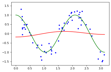
(a) Features $\{\cos(mx)\}_{m=1}^{2}$: underfitting. A linear combination of features cannot approximate the true dependence.

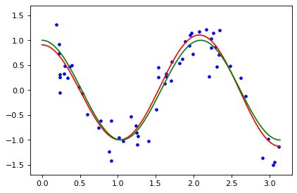
(b) Features $\{\cos(mx)\}_{m=1}^{3}$: the best fit. This is the minimum number of features that span the true dependence.

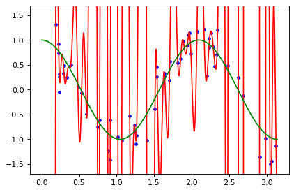
(c) Features $\{\cos(mx)\}_{m=1}^{50}$: overfitting. As the number of features approaches the number of data points, the effect of the noise becomes stronger.

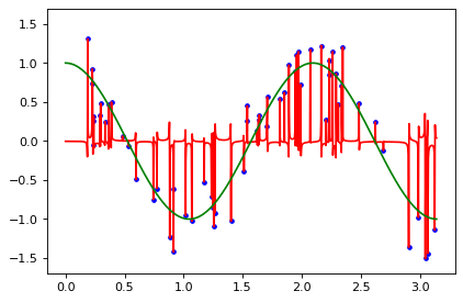
(d) Features $\{\cos(mx)\}_{m=1}^{2000}$: isotropic overparameterization. As the number of cosine features grows above the interpolation threshold, the learned solution goes to zero out of sample.

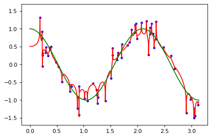
(e) Features $\{\cos(mx)/m\}_{m=1}^{2000}$: benign overfitting. Adding weights to cosine features results in interpolating the noise with high frequency features and learning the signal with low frequency features.

(f) Legend for all the plots.

Figure 1: Learning $\cos(3x)$ using linear regression with different featurizations. The data points $(x_{i},y_{i})_{i=1}^{60}$ were generated i.i.d. such that $x_{i}$ have uniform distribution on $[0,\pi]$ and $y_{i}$ have normal distribution with mean $\cos(3x_{i})$ and standard deviation $0.4$. The OLS estimator was used when $n$ is larger than the number of features, and the minimum norm interpolating solution was used otherwise.

3.2 The ground provided by the previous work

Bartlett et al. (2020) studied the variance term for ridgeless regression under the additional assumption that the data vectors have independent components. To give an overview of their results, introduce the following quantities: for any $k\in\{0,1,2,\dots,p-1\}$ define

$$r_{k}:=\frac{1}{\lambda_{k+1}}\left(\lambda+\sum_{i>k}\lambda_{i}\right),\quad\rho_{k}:=r_{k}/n.$$

In the ridgeless setting, meaning $\lambda=0$, $r_{0}$ is a well-known effective rank of the matrix $\Sigma$, $r_{k}$ is the effective rank of the same matrix, but after restricting it to the span of its last $p-k$ eigenvectors, and $\rho_{k}$ measures how large that effective rank is compared to the number of data points.

Given this notation, Bartlett et al. (2020) defined $k^{*}$ as the minimum $k$ for which $\rho_{k}$ is larger than a universal constant. Their result is then that if such a $k^{*}$ doesn’t exist or if $k^{*}/n$ is at least a constant, then $V$ is lower bounded by a constant. Otherwise, they show that with high probability $V$ is equal up to a constant factor to the following quantity:

$$\frac{k^{*}}{n}+\frac{n\sum_{i>k^{*}}\lambda_{i}^{2}}{\left(\sum_{i>k^{*}}\lambda_{i}\right)^{2}}.$$

Inspection of the proof shows that the "essentially low-dimensional" rate $k/n$ comes from the first $k$ components of the vector $\hat{\theta}(\varepsilon)$ and the term ${\left(n\sum_{i>k^{*}}\lambda_{i}^{2}\right)}/{\left(\sum_{i>k^{*}}\lambda_{i}\right)^{2}}$ comes from the rest of the components of $\hat{\theta}(\varepsilon)$. Note that if one plugs in $\lambda_{i}=\lambda_{j}$ for all $i,j>k^{*}$, then it becomes ${\left(n\sum_{i>k^{*}}\lambda_{i}^{2}\right)}/{\left(\sum_{i>k^{*}}\lambda_{i}\right)^{2}}=n/(p-k^{*})$ — exactly the variance term of the "essentially high-dimensional" regime of Section 3.1. The conclusion of Bartlett et al. (2020) is therefore that the only way that an interpolating solution can damp the noise by more than a constant factor is the following: the data is such that after removing $k$ components, it becomes "essentially high-dimensional", meaning that the effective rank of its covariance is large compared to the number of data points. After that the variance in the first $k$ components is the same as for the classical least squares, and the variance in the rest of the components corresponds to the "essentially high-dimensional" case, where you cannot learn but the noise is still damped. Note, however, that that story was not complete because only the variance term was bounded sharply in that work.

3.3 Our contribution

We complete the story of Bartlett et al. (2020) by providing sharp bounds on the bias term, extending the results to the setting of ridge regression with nonzero $\lambda$, and replacing the assumption of independence of the components by a much broader sufficient condition. From our point of view, $k^{*}$ is the main discovery of Bartlett et al. (2020). In our work we also start with separation of the first $k$ eigendirections and show that the same split leads to a bound for the bias term that is in full alignment with the intuitive explanation given above.

Let’s introduce some notation. Recall that we fixed the basis to be the eigenbasis of the covariance in (1). For any $k\in\{0,1,\dots,p\}$ we denote $X_{0:k}$ and $Z_{0:k}$ to be the matrices comprised of the first $k$ columns of $X$ and $Z$ respectively. Analogously, we denote $X_{k:\infty}$ and $Z_{k:\infty}$ to be the matrices comprised of the last $p-k$ columns of $X$ and $Z$, $\Sigma_{0:k}=\operatorname{\mathrm{diag}}(\lambda_{1},\dots,\lambda_{k})$ and $\Sigma_{k:\infty}=\operatorname{\mathrm{diag}}(\lambda_{k+1},\dots,\lambda_{p}).$ For any $\theta\in\mathbb{R}^{p}$ we denote $\theta_{0:k}$ to be the vector comprised of the first $k$ components of $\theta$, and $\theta_{k:\infty}$ — of the remaining components. We choose the ${k:\infty}$ notation instead of $k:p$ to emphasize that our results don’t depend on $p$, and only the notions of effective dimension implicitly given by the sequence $\{\lambda_{i}\}_{i=1}^{p}$ matter. For example, if one increases the dimension to $p^{\prime}>p$ and pads the sequence $\{\lambda_{i}\}_{i=1}^{p}$ with $p^{\prime}-p$ zeros, our results will still hold.

The central object in our analysis is the following matrix:

$$A_{k}:=X_{k:\infty}X_{k:\infty}^{\top}+\lambda I_{n}.$$ (3)

The matrix $X_{k:\infty}X_{k:\infty}^{\top}$ is the Gram matrix of the data after removing the first $k$ components. $A_{k}$ is obtained from that Gram matrix by shifting all eigenvalues by the ridge regularization parameter $\lambda$.

In Bartlett et al. (2020), the crucial step was to show that the singular values of $A_{k}$ are within a constant factor of each other for $k=k^{*}$ (see their Lemma 5). When the components of data vectors are independent, such control over the condition number is a consequence of high effective rank. In this paper, the roles of effective rank and condition number of $A_{k}$ are reversed. We prove sharp bounds assuming that there is some oracle that guarantees that with high probability all eigenvalues of $A_{k}$ are within a constant factor of each other. Independence of components is not needed. Moreover, such control implies that $\rho_{k}$ is at least a constant, which, in turn, implies sharpness of the bounds. In other words, we provide a more general condition under which the tail of the data is "essentially high dimensional" — instead of assuming independent components and high effective rank, only oracle control of condition number of $A_{k}$ is needed. In Section 5 we provide an extensive discussion of this assumption: we show that a version of a small-ball condition for the tails of the data is required and that a stronger version of the same condition is sufficient if the data is sub-Gaussian.

The bound that we obtain for the bias term is given informally by the following expression:

$$B\approx\|\theta^{*}_{k:\infty}\|_{\Sigma_{k:\infty}}^{2}+\|\theta_{0:k}^{*}\|_{\Sigma_{0:k}^{-1}}^{2}\left(\frac{\lambda+\sum_{i>k}\lambda_{i}}{n}\right)^{2}.$$

One can see how it aligns with the intuition of “essentially low-dimensional” and “essentially high-dimensional” parts: one cannot estimate the signal in the high dimensional part, so almost all of its energy $\|\theta^{*}_{k:\infty}\|_{\Sigma_{k:\infty}}^{2}$ goes into the error. When it comes to the low-dimensional part, the high-dimensional part acts as a ridge regularizer for it, so the bias in the first $k$ components is the same as that of ridge regression with regularization coefficient $\lambda+\sum_{i>k}\lambda_{i}$ (i.e., the full regularization is equal to the explicitly imposed part $\lambda$ plus "implicit regularization", which is equal to the energy of the tail.)

Our extension of the results to the ridge regression scenario allows us to answer the following question: can it happen that the "essentially high dimensional part" is too high dimensional, meaning that it provides too much regularization and negative $\lambda$ is needed to compensate for that? In Section 8, we show that this indeed can happen and that the following is sufficient for it to be true: the noise and the energy of the signal in the tail (components ${k:\infty}$) are small compared to the signal in the spiked part (components ${0:k}$), but the effective rank of the tail abruptly becomes much larger than $n$.

3.4 Additional notation

For any symmetric matrix $M\in\mathbb{R}^{n\times n}$ and any $i\in\{1,2,\dots,n\}$ we write $\mu_{i}(M)$ for the $i$-th largest eigenvalue of $M$. For example, $\mu_{1}(M)$ is its largest eigenvalue, and $\mu_{n}(M)$ is the smallest. We write $M[i,j]$ for the element of $M$ standing in the $i$-th row and $j$-th column.

Throughout the paper the following objects will be needed: for any $i$ denote $z_{i}$ to be the $i$-th column of $Z$. Then define

$$A_{-i}:=X_{0:i-1}X_{0:i-1}^{\top}+X_{i:\infty}X_{i:\infty}^{\top}+\lambda I_{n}=\lambda I_{n}+\sum_{j\neq i}\lambda_{j}z_{j}z_{j}^{\top},$$

an analogue of the matrix $A$, but we throw away the $i$-th component of the data vectors. Denote also

$$\rho_{k}(0)=\frac{1}{n\lambda_{k+1}}\sum_{i>k}\lambda_{i},$$

the ratio of the effective rank of the tail to the number of data points without taking regularization $\lambda$ into account.

Finally, denote our data points to be $\{x^{i}\}_{i=1}^{n}$, i.e., $X^{\top}=[x^{1},\dots,x^{n}]\in\mathbb{R}^{p\times n}$.

For the readers convenience, we compile all the notation in Appendix A.

4 Main results

As we explained in the previous section, the central objects in our proof are $A_{k}$ and $\rho_{k}$. In principle, any control of the spectrum of $A_{k}$ leads to some upper bound on $B$ and $V$ (see our Theorem 5), the question is when that bound is tight. The intuitive answer is the following: the bound is tight when the condition number of $A_{k}$ is a constant and $k$ is chosen correctly, meaning that either $\rho_{k}$ is a constant or $k$ is the smallest number such that $\rho_{k}$ is larger than a constant (i.e., $k=k^{*}$). Our arguments, however, only support this intuition when the following technical assumption holds for some constant $\gamma<1$:

1. Assume that $\lambda>-\gamma\sum_{i>k}\lambda_{i}$.

The reason why this assumption is needed is that as $\lambda$ approaches $-\sum_{i>k}\lambda_{i}$, $\mathbb{E}A_{k}$ approaches zero. It still can be possible to bound the eigenvalues of $A_{k}$ with high probability in such regime, but their magnitude will be smaller, and some error terms that were dominated before become significant. We do investigate such a regime in Section 8, where we show that negative regularization may give better rates than any value of non-negative regularization, but we only provide an upper bound there. For all the results we discuss in this section, we make Assumption NoncritReg($k,\gamma$)$(k,\gamma)$.

The focus of our work was to obtain the tight upper bound on the excess risk under minimal assumptions. Such minimal assumption turns out to be

1. Assume that with probability at least $1-\delta$ the matrix $A_{k}$ is positive-definite (PD) with condition number at most $L$.

We provide a thorough discussion of this assumption in Section 5, for example we derive sufficient and almost matching necessary conditions for it to hold when the distribution is sub-Gaussian. The reason why we don’t just assume those sufficient conditions is that we believe that sub-Gaussianity is not essential for our results to hold, as we discuss in Section 6.4. Moreover, the matrix $A_{k}$ is the central object in our argument, and making an assumption on its condition number explicitly makes presentation easier.

A careful reader will notice that we have just stated that another condition is needed for the bound to be tight: $k$ should be chosen in the right way. This, however, can be achieved by shifting $k$ to $k^{*}$ if necessary: indeed, assumptions NoncritReg($k,\gamma$)$(k,\gamma)$ and CondNum($k,\delta,L$)$(k,\delta,L)$ imply a constant lower bound on $\rho_{k}$ (see Corollary 6). That means that either $\rho_{k}$ is a constant, or it is more than a constant, i.e., $k>k^{*}$. In the latter case one can shift from $k$ to $k^{*}$ meaning that Assumption CondNum($k,\delta,L$)$(k^{*},\delta^{\prime},L^{\prime})$ also holds with modified constants $\delta^{\prime},L^{\prime}$ (see Lemma 11 for the exact statement). Now applying the upper bound (Corollary 6) with $k=k^{*}$ gives tight result, as given by the following

Theorem 1

Fix any constants $b>0,$ $\gamma\in[0,1),$ $L>0.$ Denote

$$k^{*}=\min\{\kappa:\rho_{\kappa}>b\}.$$

There exists a constant $c$ which only depends on $\sigma_{x}$, $b$, $\gamma$, $L$ such that the following holds: suppose NoncritReg($k,\gamma$)$(\bar{k},\gamma)$ and CondNum($k,\delta,L$)$(\bar{k},\delta,L)$ are satisfied for some $\bar{k}<n/c$ and $\delta<1-ce^{-n/c}$. Take $k=\min(\bar{k},k^{*})$. Then with probability at least $1-ce^{-n/c}-\delta$

$$B/c\leq \|\theta^{*}_{k:\infty}\|_{\Sigma_{k:\infty}}^{2}+\|\theta_{0:k}^{*}\|_{\Sigma_{0:k}^{-1}}^{2}\left(\frac{\lambda+\sum_{i>k}\lambda_{i}}{n}\right)^{2},$$ (4)

$$V/c\leq \frac{k}{n}+\frac{n\sum_{i>k}\lambda_{i}^{2}}{\left(\lambda+\sum_{i>k}\lambda_{i}\right)^{2}}.$$ (5)

Moreover $\rho_{k}\geq c^{-1}$, NoncritReg($k,\gamma$)$(k,\gamma)$ holds, and there exist $L^{\prime},c^{\prime}$ that only depend on $\sigma_{x},b,\gamma,L$ s.t. CondNum($k,\delta,L$)$(k,\delta+c^{\prime}e^{-n/c^{\prime}},L^{\prime})$ holds.

Proof  In this proof let’s call any quantities that only depend on $\sigma_{x}$, $\gamma$, $b$ and $L$ "constants". First of all, if $\bar{k}\leq k^{*}$ then $k=\bar{k}$. Since we are given that NoncritReg($k,\gamma$)$(\bar{k},\gamma)$ and CondNum($k,\delta,L$)$(\bar{k},\delta,L)$ are satisfied, we immediately get that NoncritReg($k,\gamma$)$(k,\gamma)$ and CondNum($k,\delta,L$)$(k,\delta+c^{\prime}e^{-n/c^{\prime}},L^{\prime})$ are satisfied with $L^{\prime}=L$ and any $c^{\prime}>0$. However, if $\bar{k}>k^{*}$ then $k=k^{*}$ and by Lemma 11 NoncritReg($k,\gamma$)$(k,\gamma)$ and CondNum($k,\delta,L$)$(k,\delta+c^{\prime}e^{-n/c^{\prime}},L^{\prime})$ are still satisfied for some constants $c^{\prime},L^{\prime}$. Note that the larger the constants, the looser the assumptions, so we can take our final choice of $c^{\prime},L^{\prime}$ to be the maximum over two cases.

Now that we know that NoncritReg($k,\gamma$)$(k,\gamma)$ and CondNum($k,\delta,L$)$(k,\delta+c^{\prime}e^{-n/c^{\prime}},L^{\prime})$ are satisfied, by Corollary 6, there is a constant $c_{1}$ such that $\rho_{k}>1/c_{1}$ and with probability at least $1-c_{1}e^{-n/c_{1}}-c^{\prime}e^{-n/c^{\prime}}-\delta$

$$B/c_{1}\leq \|\theta^{*}_{k:\infty}\|_{\Sigma_{k:\infty}}^{2}+\|\theta_{0:k}^{*}\|_{\Sigma_{0:k}^{-1}}^{2}\left(\frac{\lambda+\sum_{i>k}\lambda_{i}}{n}\right)^{2},$$

$$V/c_{1}\leq \frac{k}{n}+\frac{n\sum_{i>k}\lambda_{i}^{2}}{\left(\lambda+\sum_{i>k}\lambda_{i}\right)^{2}}.$$

Taking $c\geq c_{1}+c^{\prime}$ gives the first part.  

Algebraically, under Assumption CondNum($k,\delta,L$)$(k,\delta,L)$ all eigenvalues of $A_{k}^{-1}$ are within a constant factor of each other, so one can pull its operator norm from the expressions and obtain an upper bound without losing tightness. This strategy, however, doesn’t produce lower bounds, so we derive them in a different way: we decompose bias and variance into sums with respect to individual coordinates of the predictor, and bound each term in each sum from below. Because of that, we impose different assumptions, namely

1. Assume that all elements of matrix $X$ are independent (i.e., data vectors have independent coordinates).

for the variance term, and

1. Assume that the sequence of coordinates of $\Sigma^{-1/2}x$ is exchangeable (any deterministic permutation of the coordinates of whitened data vectors doesn’t change their distribution).

2. Assume that $\theta^{*}$ is sampled from a prior distribution in the following way: one starts with vector $\bar{\theta}$ and flips signs of all its coordinates with probability $0.5$ independently.

for the bias term. Because of this mismatch in assumptions, our lower bounds don’t show that our upper bound is always tight. What they show is that one needs some specific knowledge about the distribution to obtain better bounds. We provide a more detailed discussion of the relations between those assumptions in Section 6.2. The lower bounds themselves are given by the following

Theorem 2

Fix any constants $b>a>0$, $\gamma\in[0,1),$ $L>0.$ Denote

$$k^{*}=\min\{\kappa:\rho_{\kappa}>b\}.$$

There exists a constant $c$ which only depends on $\sigma_{x}$, $a$, $b$, $\gamma$, $L$ such that all the following hold:

1. For any $k\in\{0,1,\dots,k^{*}\}$ under assumptions IndepCoord, NoncritReg($k,\gamma$)$(k,\gamma)$, if $\rho_{k}>a$ then with probability at least $1-2\delta-ce^{-c/n}$

   $$V\geq\frac{1}{c}\left(\frac{k}{n}+\frac{n\sum_{i>k}\lambda_{i}^{2}}{\left(\lambda+\sum_{i>k}\lambda_{i}\right)^{2}}\right).$$

2. For any $k\in\{1,2,\dots,k^{*}\}$ under assumptions NoncritReg($k,\gamma$)$(k,\gamma)$, CondNum($k,\delta,L$)$(k,\delta,L)$, PriorSigns($\bar{\theta}$)$(\bar{\theta})$ and ExchCoord, if $\rho_{k}>a$ then with probability at least $1-2\delta-ce^{-c/n}$

   $$\mathbb{E}_{\theta^{*}}B\geq\frac{1}{c}\left(\|\bar{\theta}_{k:\infty}\|_{\Sigma_{k:\infty}}^{2}+\|\bar{\theta}_{0:k}\|_{\Sigma_{0:k}^{-1}}^{2}\left(\frac{\lambda+\sum_{i>k}\lambda_{i}}{n}\right)^{2}\right),$$

   where $\mathbb{E}_{\theta^{*}}$ denotes expectation over a random draw of $\theta^{*}$ from the distribution described in assumption PriorSigns($\bar{\theta}$)$(\bar{\theta})$.

Proof  Lemma 7 gives a lower bound for $V$, and Lemmas 8 and 9 give the lower bound for B. Those lower bounds have the desired probability, but different algebraic form. To bring them to the same form as the upper bounds one needs the right $k$ to be chosen. We assumed that $\rho_{k}>a$. Moreover, since $k\leq k^{*}$ by definition of $k^{*}$ we either have $\rho_{k}\leq b$ or $k=k^{*}$. In both of those cases Theorem 10 guarantees that these lower bounds are the same as what we need up to multiplicative constants that only depend on $\sigma_{x}$, $\gamma$, $a$, $b$ and $L$.  

One can notice from this proof that having separate arguments for the lower bounds results in a different algebraic form of the same bound. This different form turns out to be convenient to draw explicit connections between our results and results from earlier works. We do that in Section 7.

5 Effective ranks and control of the spectrum of $A_{k}$

The central assumption that we need to compute the excess risk is Assumption CondNum($k,\delta,L$)$(k,\delta,L)$, which provides control over condition number of $A_{k}$. In this section we discuss when this assumption is known to be satisfied and what are the necessary conditions for it to happen.

5.1 Effect of $\lambda$ on the condition number

Recall that $A_{k}=X_{k:\infty}X_{k:\infty}^{\top}+\lambda I_{n}$, so its spectrum is the shift by $\lambda$ of the spectrum of $X_{k:\infty}X_{k:\infty}^{\top}$, the random matrix that is equal to the Gram matrix of the projected data. There are therefore three ways of establishing a constant upper bound on the condition number of $A_{k}$:

1. Establish an upper bound $\bar{\mu}$ on $\mu_{1}(X_{k:\infty}X^{\top}_{k:\infty})$ and take $\lambda>\bar{\mu}/c$ for some constant $c>0$. In this case, the singular values of $A_{k}$ are all equal to $\lambda$ (and greater than $\bar{\mu}$) up to a constant multiplier.

2. Establish upper and lower bounds $\bar{\mu}$ and $\underline{\mu}$ on $\mu_{1}(X_{k:\infty}X^{\top}_{k:\infty})$ and $\mu_{n}(X_{k:\infty}X^{\top}_{k:\infty})$ respectively, such that $\bar{\mu}/\underline{\mu}$ is a constant. Then take $\lambda>-\underline{\mu}/c$ for some constant $c>1$. In this case, the singular values of $A_{k}$ are all equal to $\bar{\mu}$ (or $\underline{\mu}$) up to a constant multiplier.

3. Establish upper and lower bounds $\bar{\mu}$ and $\underline{\mu}$ on $\mu_{1}(X_{k:\infty}X^{\top}_{k:\infty})$ and $\mu_{n}(X_{k:\infty}X^{\top}_{k:\infty})$ respectively, and take $\lambda=-\underline{\mu}+\Diamond$, where $\Diamond\geq c(\bar{\mu}-\underline{\mu})$ for a constant $c>0$. In this case, the singular values of $A_{k}$ are all equal to $\Diamond$ up to a constant multiplier. This case can be substantially different from the previous case when the singular values of $X_{k:\infty}X^{\top}_{k:\infty}$ are very well concentrated, i.e., the gap $\bar{\mu}-\underline{\mu}$ is of smaller order than $\underline{\mu}$ itself. In this case $\Diamond$ can be a smaller order term.

Our bounds are sharp when assumption NoncritReg($k,\gamma$)($\gamma$) is satisfied for some $\gamma<1$, i.e., in the first and the second case above. The third case is quite rare because it requires very good concentration of the spectrum of $X_{k:\infty}X^{\top}_{k:\infty}$. Moreover, in this case $\lambda$ is very close to the critical negative value under which it is impossible to even guarantee that $A_{k}$ is PD as it becomes negative definite in expectation. We use this regime to investigate how negative regularization can improve excess risk by more than a constant factor in Section 8. However, we don’t expect our bounds to always be sharp in this regime.

Therefore, we focus our attention on the first two cases. In Section 5.2 we discuss informally what conditions on the distribution are necessary to bound $\mu_{1}(X_{k:\infty}X^{\top}_{k:\infty})$ and $\mu_{n}(X_{k:\infty}X^{\top}_{k:\infty})$, and show how notions of high effective rank and norm concentration condition arise. In Section 5.3 we combine those bounds for sub-Gaussian data with the choice of $\lambda$ to provide necessary and almost matching sufficient conditions for the condition number of $A_{k}$ to be constant under sub-Gaussianity. In Section 5.4 we show that sub-Gaussianity is not actually required for the condition number of $A_{k}$ to be controlled with high probability: Theorem 4 states that norm concentration condition and a modified version of high effective rank condition are sufficient even if the data only has bounded $4+\varepsilon$ moments.

5.2 Informal necessary conditions

There are several easy observations that help understand what is needed for the condition number of $A_{k}$ to be bounded.

1. The first observation is that $X_{k:\infty}X^{\top}_{k:\infty}\succeq\lambda_{k+1}z_{k+1}z_{k+1}^{\top}$, where $z_{k+1}$ is the first column of $Z_{k:\infty}$ —a vector with $n$ i.i.d. coordinates with unit variance. By the law of large numbers, $\|z_{k+1}\|^{2}\approx n$, meaning that $\|\lambda_{k+1}z_{k+1}z_{k+1}^{\top}\|\approx\lambda_{k+1}n$. Therefore, $\bar{\mu}\gtrsim\lambda_{k+1}n$.

2. The second observation is that the diagonal elements of $X_{k:\infty}X^{\top}_{k:\infty}$ are squared norms of the tails of data vectors. Recall that we denoted the data points to be $\{x^{i}\}_{i=1}^{n}$. We can write

   $$(X_{k:\infty}X^{\top}_{k:\infty})[i,i]=\|x^{i}_{k:\infty}\|^{2}\text{ --- i.i.d. r.v's.}$$

   Once again, by the law of large numbers, $\operatorname{\mathrm{tr}}(X_{k:\infty}X^{\top}_{k:\infty})\approx n\sum_{i>k}\lambda_{i},$ which implies that $\bar{\mu}\gtrsim\sum_{i>k}\lambda_{i}\gtrsim\underline{\mu}$. Combining it with the first observation shows that $\bar{\mu}$ and $\underline{\mu}$ can only be within a constant multiplier of each other when $\sum_{i>k}\lambda_{i}\geq c\lambda_{k+1}n$ for some constant $c$. This is exactly the high effective rank condition $\rho_{k}>c$ for $\lambda=0$.

3. The third observation is that the diagonal elements of a PD matrix themselves provide bounds on the singular values:

   $$\mu_{n}(X_{k:\infty}X^{\top}_{k:\infty})\leq\min_{i\in[n]}(X_{k:\infty}X^{\top}_{k:\infty})[i,i]\leq\max_{i\in[n]}(X_{k:\infty}X^{\top}_{k:\infty})[i,i]\leq\mu_{1}(X_{k:\infty}X^{\top}_{k:\infty}).$$

   Therefore, to control condition number of $X_{k:\infty}X^{\top}_{k:\infty}$ by a constant $L$ with probability $1-\delta$, it is necessary to guarantee that

   $$\max_{i}\|x^{i}_{k:\infty}\|^{2}\leq L\min_{j}\|x^{j}_{k:\infty}\|^{2},$$

   i.e., $n$ independent random draws of the random variable $\|x_{k:\infty}\|^{2}$ should all lie within a constant factor of some value, meaning that the norm of the tail of a data vector should be within a constant factor of a fixed value with probability $(1-\delta)^{1/n}$.

5.3 Controlling condition number under sub-Gaussianity

Sub-Gaussianity of the data implies an upper bound on $\mu_{1}(A_{k})$, but doesn’t help with $\mu_{n}(A_{k})$. To see this one can consider a well-known construction: take a sub-Gaussian distribution and construct another distribution in the following way: to sample from this new distribution take a vector from the old distribution and multiply it by $\sqrt{2}$ with probability $1/2$ and by zero otherwise. The new distribution is still sub-Gaussian with the same covariance, but the Gram matrix of $n$ i.i.d. samples from it is degenerate with probability at least $1-2^{-n}$. Therefore, an additional assumption is needed to lower bound $\mu_{n}(A_{k})$. As we already mentioned in Section 5.2, we need norm concentration. Since sub-Gaussianity allows to bound the norm from above, it reduces to a version of the small-ball condition: $\|x_{k:\infty}\|$ should be lower-bounded with high probability. The formal result is given by the following

Lemma 3 (Controlling $\mu_{1}(A_{k})/\mu_{n}(A_{k})$ under sub-Gaussianity)

For any $\gamma\in[0,1)$ and $\sigma_{x}>0$ there exists $c>0$ that only depends on $\sigma_{x}$ and $\gamma$ such that under Assumption NoncritReg($k,\gamma$)$(k,\gamma)$ the following holds: for any $L\geq 1$

• If $\rho_{k}\geq L^{2}$ and with probability at least $(1-\delta)^{1/n}$

  $$\lambda+\|x_{k:\infty}\|^{2}\geq\frac{c}{L}\left(\lambda+\mathbb{E}\|x_{k:\infty}\|^{2}\right),$$

  then with probability at least $1-\delta-ce^{-n/c}$

  $$\mu_{n}(A_{k})\geq L^{-1}\mu_{1}(A_{k}).$$

• Suppose that it is known that with probability at least $ce^{-n/c}$ $\mu_{n}(A_{k})\geq L^{-1}\mu_{1}(A_{k})$. Then $\rho_{k}\geq\frac{1}{cL}$ and with probability at least $\left(1-ce^{-n/c}\right)^{1/n}$

  $$\lambda+\|x_{k:\infty}\|^{2}\geq\frac{1}{cL}\left(\lambda+\mathbb{E}\|x_{k:\infty}\|^{2}\right).$$

The proof is given in Appendix D. One can see that both the necessary and the sufficient conditions are that $\rho_{k}$ is lower bounded by a constant and a version of small-ball condition that says that the regularized squared norm of the data exceeds a constant fraction of its expectation with probability $(1-\delta)^{1/n}$. There is, however, a gap in those constants.

5.4 Heavy-tailed case

The following is a direct corollary of Theorem 2.1 from Guédon et al. (2017)

Theorem 4

Suppose that the distribution of the tail satisfies the following two assumptions:

1. Norm concentration: For some $\delta\in(0,1/n)$, $L>1$ and $M>0$

   $$\mathbb{P}(L^{-1}\leq\|x_{k:\infty}\|/M\leq L)\geq 1-\delta.$$

2. Heavy-tailed effective rank: for some $h>4$ denote $r_{h,k}>0$ to be the maximum number such that for any $a\in\mathcal{S}^{p-k-1}$ and $t>0$

   $$\mathbb{P}\left(\frac{\sqrt{r_{h,k}}\left|a^{\top}x_{k:\infty}\right|}{M}>t\right)\leq t^{-h}.$$

There exists a constant $c$ that only depends on $h$ such that with probability at least $1-cn^{1-h/4}-n\delta$

$$\mu_{1}(X_{k:\infty}X_{k:\infty}^{\top})\leq M^{2}\left(L^{2}+cL^{2}\left(n^{1-h/4}+\sqrt{\frac{n}{r_{h,k}L^{2}}}+\frac{n}{r_{h,k}L^{2}}\right)\right),$$

$$\mu_{n}(X_{k:\infty}X_{k:\infty}^{\top})\geq M^{2}\left(L^{-2}-cL^{2}\left(n^{1-h/4}+\sqrt{\frac{n}{r_{h,k}L^{2}}}+\frac{n}{r_{h,k}L^{2}}\right)\right).$$

Proof  First, note that by union bound with probability at least $1-n\delta$ all the diagonal elements of the matrix $X_{k:\infty}X_{k:\infty}^{\top}$ belong to the segment $[L^{-2}M^{2},L^{2}M^{2}]$. Next, take the bound on $B_{k}$ from the Case 1 of Theorem 2.1 from Guédon et al. (2017) with the following choice of their parameters: $k=N$, $\tau=1$, $\lambda=p$, $\sigma=1+p/4$, $t=\sqrt{n}$. Use that bound for vectors $\sqrt{r_{h,k}}x^{i}_{k:\infty}/M$. Note that that $B_{k}$ is exactly the operator norm of the off-diagonal part of $r_{h,k}X_{k:\infty}X_{k:\infty}^{\top}/M^{2}$.  

The quantity $r_{h,k}$ that we introduced in Theorem 4 can be interpreted as a notion of effective rank for heavy tailed distributions. Indeed, one can write

$$\sqrt{r_{h,k}}=\frac{M}{\inf\left\{\tau:\forall a\in\mathcal{S}^{p-k-1}\forall t>0\;\mathbb{P}\left(\left|a^{\top}x_{k:\infty}\right|/\tau>t\right)\leq t^{-h}\right\}}.$$

— the ratio of the typical norm of the random vector to the scale of the worst case deviations of its one-dimensional projection. This is completely analogous to our usual definition of the effective rank: $r_{k}=\lambda_{k+1}^{-1}\sum_{i>k}\lambda_{i}$. Indeed, in sub-Gaussian case $\sqrt{\sum_{i>k}\lambda_{i}}$ is the typical value of the norm of the vector $x_{k:\infty}$, and $\sqrt{\lambda_{k+1}}$ is up to constant the largest sub-Gaussian norm of its one-dimensional projection. We see that the conditions under which the eigenvalues of $X_{k:\infty}X_{k:\infty}^{\top}$ are within a constant factor of each other with high probability remain the same even in the heavy-tailed case: the norm of $\|x_{k:\infty}\|$ concentrates within a constant factor of a fixed quantity, and the heavy-tailed effective rank $r_{h,k}$ should be large compared to the number $n$ of data points.

6 Structure of the proof and role of sub-Gaussianity

6.1 Upper bound

The core of our argument is Theorem 5 given below. There are two important things to note about it: first, it only requires sub-Gaussianity and matrix $A_{k}$ being positive semidefinite (which always holds with probability $1$ for non-negative $\lambda$). Second, its proof decomposes very clearly into two parts: an algebraic part, which only requires $A_{k}$ being PD and holds with probability $1$ conditionally on this event, and a probabilistic part, where standard concentration results are directly plugged into the algebraic bounds. Because of this decomposition, it is straightforward to track how the sub-Gaussianity is used and how it can be relaxed. We provide the sketch of the proof to show these details.

Theorem 5

There exists a (large) constant $c$, which only depends on $\sigma_{x}$, s.t. for any $k<n/c$ with probability at least $1-ce^{-n/c}$, if the matrix $A_{k}$ is PD, then

$$B/c\leq \|\theta^{*}_{k:\infty}\|_{\Sigma_{k:\infty}}^{2}\left(1+\frac{\mu_{1}(A_{k}^{-1})^{2}}{\mu_{n}(A_{k}^{-1})^{2}}+n\lambda_{k+1}\mu_{1}(A_{k}^{-1})\left(1+\max(0,-\lambda)\mu_{1}(A_{k}^{-1})\right)\right)$$

$$+ \|\theta_{0:k}^{*}\|_{\Sigma_{0:k}^{-1}}^{2}\left(\frac{1}{n^{2}\mu_{n}(A_{k}^{-1})^{2}}+\frac{\lambda_{k+1}}{n}\frac{\mu_{1}(A_{k}^{-1})}{\mu_{n}(A_{k}^{-1})^{2}}\left(1+\max(0,-\lambda)\mu_{1}(A_{k}^{-1})\right)\right),$$

$$V/c\leq \frac{\mu_{1}(A_{k}^{-1})^{2}}{\mu_{n}(A_{k}^{-1})^{2}}\frac{k}{n}+n\mu_{1}(A_{k}^{-1})^{2}\sum_{i>k}\lambda_{i}^{2}.$$

Proof sketch  The full proof of Theorem 5 can be found in Section I.1 of the appendix. The following is a sketch of its derivation.

Recall the following notation: for any $y$

$$\hat{\theta}(y)=X^{\top}(\lambda I_{n}+XX^{\top})^{-1}y.$$

As explained in Section 3.2, Bartlett et al. (2020) introduced the notion of $k^{*}$ for which the behaviour of the variance term in the first $k^{*}$ coordinates is qualitatively different than in the rest of the coordinates. Their argument, however, relies crucially on independence of the components of the data. The main idea that allowed us to get rid of that assumption and to obtain the tight bound for the bias term was to separate the first $k$ coordinates from the very beginning and to use some sort of uniform convergence argument in that low-dimensional subspace.

The crucial tool that allowed us to realise this idea turned out to be the following algebraic identity that we prove in Section F of the appendix:

$$\hat{\theta}(y)_{0:k}+X_{0:k}^{\top}A_{k}^{-1}X_{0:k}\hat{\theta}(y)_{0:k}=X_{0:k}^{\top}A_{k}^{-1}y.$$

This identity allows convenient access to the error in the first $k$ coordinates (the spiked part).

The argument decomposes clearly into two parts: algebraic and probabilistic. The algebraic part is to decompose the excess risk (up to a constant multiplier) into four terms and show that the following inequalities hold on the event that the matrix $A_{k}$ is PD:
(1) Bias error in the spiked part:

$$\|\hat{\theta}(X\theta^{*})_{0:k}-\theta^{*}_{0:k}\|_{\Sigma_{0:k}}\leq \frac{\mu_{1}(A_{k}^{-1})}{\mu_{n}(A_{k}^{-1})}\frac{\mu_{1}\left(\Sigma^{-1/2}_{0:k}X_{0:k}^{\top}X_{0:k}\Sigma_{0:k}^{-1/2}\right)^{1/2}}{\mu_{k}\left(\Sigma^{-1/2}_{0:k}X_{0:k}^{\top}X_{0:k}\Sigma_{0:k}^{-1/2}\right)}\|X_{k:\infty}\theta^{*}_{k:\infty}\|$$

$$\qquad{}+\frac{\|\theta_{0:k}^{*}\|_{\Sigma_{0:k}^{-1}}}{\mu_{n}(A_{k}^{-1})\mu_{k}\left(\Sigma^{-1/2}_{0:k}X_{0:k}^{\top}X_{0:k}\Sigma_{0:k}^{-1/2}\right)}.$$

(2) Variance error in the spiked part:

$$\mathbb{E}_{\varepsilon}\|\hat{\theta}(\varepsilon)_{0:k}\|_{\Sigma_{0:k}}^{2}\leq\frac{\mu_{1}(A_{k}^{-1})^{2}\|X_{0:k}\Sigma_{0:k}^{-1/2}\|^{2}}{\mu_{n}(A_{k}^{-1})^{2}\mu_{k}\left(\Sigma_{0:k}^{-1/2}X_{0:k}^{\top}X_{0:k}\Sigma_{0:k}^{-1/2}\right)^{2}}.$$

(3) Variance error in the tail:

$$\mathbb{E}_{\varepsilon}\|\hat{\theta}(\varepsilon)_{k:\infty}-\theta^{*}_{k:\infty}\|_{\Sigma_{k:\infty}}^{2}\leq\mu_{1}(A_{k}^{-1})^{2}\operatorname{\mathrm{tr}}(X_{k:\infty}\Sigma_{k:\infty}X_{k:\infty}^{\top}).$$

(4) Bias error in the tail:

$$\frac{1}{3}\|\hat{\theta}(X\theta^{*})_{k:\infty}-\theta^{*}_{k:\infty}\|_{\Sigma_{k:\infty}}^{2}$$

$$\leq \|\theta^{*}_{k:\infty}\|_{\Sigma_{k:\infty}}^{2}+\lambda_{k+1}\bigl{(}1+\max(0,-\lambda)\mu_{1}(A_{k}^{-1})\bigr{)}\mu_{1}(A_{k}^{-1})\|X_{k:\infty}\theta^{*}_{k:\infty}\|^{2}$$

$$+ \lambda_{k+1}\bigl{(}1+\max(0,-\lambda)\mu_{1}(A_{k}^{-1})\bigr{)}\frac{\mu_{1}(A_{k}^{-1})}{\mu_{n}(A_{k}^{-1})^{2}}\frac{\mu_{1}(\Sigma_{{0:k}}^{-1/2}X_{0:k}^{\top}X_{0:k}\Sigma_{{0:k}}^{-1/2})}{\mu_{k}(\Sigma_{{0:k}}^{-1/2}X_{0:k}^{\top}X_{0:k}\Sigma_{{0:k}}^{-1/2})^{2}}\|\Sigma_{{0:k}}^{-1/2}\theta^{*}_{0:k}\|^{2}.$$

The probabilistic part of the argument is to control the quantities that arise in the algebraic bound with high probability. Namely, we plug in

• Concentration of $k$-dimensional sample covariance with $n$ samples: w.h.p.

  $$\mu_{k}\left(\frac{1}{n}\Sigma_{0:k}^{-1/2}X_{0:k}^{\top}X_{0:k}\Sigma_{0:k}^{-1/2}\right)\approx_{\sigma_{x}}\mu_{1}\left(\frac{1}{n}\Sigma_{0:k}^{-1/2}X_{0:k}^{\top}X_{0:k}\Sigma_{0:k}^{-1/2}\right)\approx_{\sigma_{x}}1.$$

• Concentration of norm of vectors with i.i.d. components: w.h.p.

  $$\frac{1}{n}\|X_{0:k}\Sigma_{0:k}^{-1/2}\|^{2}\lesssim_{\sigma_{x}}k,\quad\frac{1}{n}\|X_{k:\infty}\Sigma_{k:\infty}^{1/2}\|^{2}\lesssim_{\sigma_{x}}\sum_{i>k}\lambda_{i}^{2},\quad\frac{1}{n}\|X_{k:\infty}\theta^{*}_{k:\infty}\|^{2}\lesssim_{\sigma_{x}}\|\theta^{*}_{k:\infty}\|_{\Sigma_{k:\infty}}^{2}.$$

After plugging in the probabilistic bounds, the final result is obtained by a straightforward computation.  

Note that the only probabilistic statements that are used in this proof are concentration of sample covariance in dimension $k$ and concentration of the sum of $n$ i.i.d. random variables. The same concentration results hold with weaker assumptions, but with larger probability. For example, under rather weak moment assumptions only a linear in dimension number of samples is needed for the sample covariance matrix to concentrate within a constant factor of the population covariance, see Tikhomirov (2017) and references therein. It is also interesting to point out that the "uniform convergence" result that we mentioned in the beginning of this sketch is nothing but the convergence of the empirical covariance matrix $\Sigma_{0:k}^{-1/2}X_{0:k}^{\top}X_{0:k}\Sigma_{0:k}^{-1/2}/n$ to its expectation $I_{k}$, which is exactly the uniform convergence result that gives the bound in the "essentially low-dimensional" regime from Section 3.1.

Despite the fact that the bounds of Theorem 5 apply under very general assumptions, we don’t expect them to be tight if the condition number of $A_{k}$ is not bounded by a constant. When some oracle control of the condition number of $A_{k}$ is provided, the bound becomes the following.

Corollary 6

Fix any constants $\gamma\in[0,1)$ and $L>0$. There exists a constant $c$ that only depends on $\sigma_{x}$, $\gamma$, $L$ s.t. for any $k<n/c$ and $\delta<1-ce^{-n/c}$ under assumptions NoncritReg($k,\gamma$)$(k,\gamma)$ and CondNum($k,\delta,L$)$(k,\delta,L)$, it holds that $\rho_{k}>c^{-1}$, and with probability at least $1-\delta-ce^{-n/c}$,

$$B/c\leq \|\theta^{*}_{k:\infty}\|_{\Sigma_{k:\infty}}^{2}+\|\theta_{0:k}^{*}\|_{\Sigma_{0:k}^{-1}}^{2}\left(\frac{\lambda+\sum_{i>k}\lambda_{i}}{n}\right)^{2},$$

$$V/c\leq \frac{k}{n}+\frac{n\sum_{i>k}\lambda_{i}^{2}}{\left(\lambda+\sum_{i>k}\lambda_{i}\right)^{2}}.$$

Proof sketch  Assumptions NoncritReg($k,\gamma$)$(k,\gamma)$ and CondNum($k,\delta,L$)$(k,\delta,L)$ imply that all the eigenvalues of $A_{k}$ are equal to $\lambda+\sum_{i>k}\lambda_{i}$ up to a multiplicative constant that depends on $L,\gamma,\sigma_{x}$. Plugging it into Theorem 5 gives the result. The full proof is given in Appendix I.1.  
The sub-Gaussianity is used in Corollary 6 to ensure that $\operatorname{\mathrm{tr}}(A_{k})$ concentrates around $n\left(\lambda+\sum_{i>k}\lambda_{i}\right)$. Since the diagonal elements of $A_{k}$ are i.i.d. random variables, the same concentration would also hold under weaker assumptions with lower but still high probability.

It is also worth mentioning that the story about "essentially high-dimensional" and "essentially low-dimensional" parts is not just an interpretation of the final result: the whole proof strategy is in accordance with it, as we explicitly separate the two parts and bound errors in them separately.

6.2 Lower bounds

Our lower bounds have a different form from the upper bounds. We show separately that they match if the condition on effective rank is satisfied. One benefit of this approach is that the lower bounds provide a different form of the same result, which allows for different analysis. We employ it in Section 7.

The lower bound for the variance term is given by the following lemma, whose proof is given in Appendix E.1:

Lemma 7 (Lower bound for the variance term)

Fix any constant $\gamma\in[0,1)$. There exists a constant $c$ that only depends on $\sigma_{x}$ and $\gamma$ s.t. for any $k<n/c$ under assumptions NoncritReg($k,\gamma$)$(k,\gamma)$ and IndepCoord w.p. at least $1-ce^{-n/c}$

$$V\geq\frac{1}{cn}\sum_{i=1}\min\left\{1,\frac{\lambda_{i}^{2}}{\lambda_{k+1}^{2}(\rho_{k}+1)^{2}}\right\}.$$

One can see that the assumptions under which the lower bound is proved are different from the assumptions required for the upper bound: we require independent components here. On the one hand, it means that there could be a gap between upper and lower bounds in some particular cases where one can control the condition number of $A_{k}$ without independence of components. On the other hand, it means that even such strong additional assumption as independence of components does not allow the upper bounds to be improved, which suggests that those specific cases for which the bound is not tight are rare and require even stronger additional assumptions.

The most general lower bound for the bias term that we prove requires the following assumption

1. Assume that for any $j\in\{1,2,\dots,p\}$ with probability at least $1-\delta$

   $$\mu_{n}(A_{-j})\geq\mu_{n}(\mathbb{E}A_{k})/L=\left(\sum_{i>k}\lambda_{i}+\lambda\right)/L,$$

   and that $\lambda>-\sum_{i>k}\lambda_{i}$.

Then the bound is given by the following lemma, whose proof is given in Appendix E.2

Lemma 8 (Lower bound for the bias term)

Fix any constant $L>0$. There exists $c$ that only depends on $\sigma_{x}$ and $L$ s.t. for any $k\in\{1,2,\dots,p\}$ under assumptions PriorSigns($\bar{\theta}$)$(\bar{\theta})$ and StableLowerEig($k,\delta,L$)$(k,\delta,L)$ w.p. at least $1-2\delta-ce^{-n/c}$

$$\mathbb{E}_{\theta^{*}}B\geq\frac{1}{c}\sum_{i}\frac{\lambda_{i}\bar{\theta}^{2}_{i}}{\left(1+\frac{\lambda_{i}}{\lambda_{k+1}\rho_{k}}\right)^{2}},$$

where $\mathbb{E}_{\theta^{*}}$ denotes the expectation over the random draw of $\theta^{*}$ from the prior distribution described in assumption PriorSigns($\bar{\theta}$)$(\bar{\theta})$.

Assumption StableLowerEig($k,\delta,L$)$(k,\delta,L)$ is formally not comparable to Assumption CondNum($k,\delta,L$)$(k,\delta,L)$, but informally if $k\geq 1$ then StableLowerEig($k,\delta,L$)$(k,\delta,L)$ is weaker: indeed, the matrix $A_{-i}$ is obtained from the matrix $A$ by subtracting $\lambda_{i}z_{i}^{\top}z_{i}$, while the matrix $A_{k}$ is obtained from $A$ by subtracting $\sum_{i=1}^{k}\lambda_{i}z_{i}^{\top}z_{i}$, i.e., the sum of $k$ "largest" of the terms $\lambda_{i}z_{i}^{\top}z_{i}$. Therefore, the matrix $A_{-i}$ is "larger" than $A_{k}$, and controlling its lowest singular value should be easier. The following lemma, whose proof is given in Appendix E.2, formalizes this argument under Assumption ExchCoord:

Lemma 9

For any $\gamma<1$ there exists a constant $c$ that only depends on $\gamma$ and $\sigma_{x}$ such that if assumptions CondNum($k,\delta,L$)$(k,\delta,L)$, NoncritReg($k,\gamma$)$(k,\gamma)$ and ExchCoord are satisfied for some $L\geq 1$ and $k\in\{1,2,\dots,p\}$, then StableLowerEig($k,\delta,L$)$(k,\delta+2e^{-n/c},cL)$ is also satisfied.

When it comes to averaging over the prior given by the assumption PriorSigns($\bar{\theta}$)$(\bar{\theta})$, it just means that it is impossible to obtain a better lower bound without some specific knowledge of how signs of components of $\theta^{*}$ interact with the probability distribution of the data.

6.3 Connecting upper and lower bounds

One slight inconvenience with our approach of imposing oracle control over the spectrum of $A_{k}$ via Assumption CondNum($k,\delta,L$)$(k,\delta,L)$ is the following: what if the oracle provides control for the wrong value of $k$? There can in principle be many values of $k$ for which such oracle control is possible, with not all of them giving the right point where the behaviour changes from "essentially low-dimensional" to "essentially high-dimensional". As an example, consider the isotropic setting with $p\gg n$: one can exclude any number $k$ of components such that $p-k\gg n$ and still be able to control the condition number.

First of all, in accordance with the result of Bartlett et al. (2020), the following theorem shows that the "right $k$" is the $k$ that is not larger than $k^{*}$.

Theorem 10 (The lower bound is the same as the upper bound)

Denote

$$\underline{B} :=\sum_{i}\frac{\lambda_{i}|\theta^{*}_{i}|^{2}}{\left(1+\frac{\lambda_{i}}{\lambda_{k+1}\rho_{k}}\right)^{2}},$$

$$\overline{B} :=\|\theta^{*}_{k:\infty}\|_{\Sigma_{k:\infty}}^{2}+\|\theta_{0:k}^{*}\|_{\Sigma_{0:k}^{-1}}^{2}\left(\frac{\lambda+\sum_{i>k}\lambda_{i}}{n}\right)^{2},$$

$$\underline{V} :=\frac{1}{n}\sum_{i}\min\left\{1,\frac{\lambda_{i}^{2}}{\lambda_{k+1}^{2}(\rho_{k}+1)^{2}}\right\},$$

$$\overline{V} :=\frac{k}{n}+\frac{n\sum_{i>k}\lambda_{i}^{2}}{\left(\lambda+\sum_{i>k}\lambda_{i}\right)^{2}}.$$

Fix constants $a>0$ and $b>1/n$. There exists a constant $c>0$ that only depends on $a,b$, s.t. the following holds: if either $\rho_{k}\in(a,b)$ or $k=\min\{\kappa:\rho_{\kappa}>b\}$, then

$$c^{-1}\leq{\underline{B}}\mathbin{/}{\overline{B}}\leq 1,\quad c^{-1}\leq{\underline{V}}\mathbin{/}{\overline{V}}\leq 1.$$

Proof  The proof is a rather straightforward comparison of pairs of sums term by term. It is given in Appendix I.2.  

Secondly, if the data is sub-Gaussian, then oracle control for any $k<n$ results in tight bounds, but with worse constants. This happens because of the following lemma.

Lemma 11 ($k$ can be taken to be $k^{*}$)

Fix any constants $\gamma\in[0,1)$, $b>0$, $L>0$. Denote

$$k^{*}=\min\{k:\rho_{k}>b\}.$$

There exist constants $c,L^{\prime}$ that only depend on $\sigma_{x}$, $\gamma$, $b$, $L$ s.t. the following holds: suppose assumptions NoncritReg($k,\gamma$)$(k,\gamma)$ and CondNum($k,\delta,L$)$(k,\delta,L)$ hold for some $k\in[k^{*},n]$. Then assumptions NoncritReg($k,\gamma$)($k^{*},\gamma$) and CondNum($k,\delta,L$)$(k^{*},\delta+ce^{-n/c},L^{\prime})$ hold too.

Proof sketch  Since $k\geq k^{*}$, $\mu_{n}(A_{k})$ provides a lower bound for $\mu_{n}(A_{k^{*}})$. When it comes to $\mu_{1}(A_{k^{*}})$, it can be bounded with high-probability because the data is sub-Gaussian. The full proof is given in Appendix D.  

6.4 The role of sub-Gaussianity

As can be seen from the proof of Theorem 1, the strategy to obtain a tight bound is the following: ask the oracle to control the condition number of $A_{k}$, if that $k$ is too large, shift it to $k^{*}$, and then apply the bound from Corollary 6. In Section 5.4 we showed that if the norm $\|x_{k:\infty}\|$ concentrates, and the effective rank $r_{h,k}$ is high enough, then the control over the condition number of $A_{k}$ is possible even if we have very weak moment assumptions instead of sub-Gaussianity. Moreover, as we have discussed in the proof sketches, if we didn’t shift from $k$ to $k^{*}$, we would only need the usual concentration results such as the law of large numbers or concentration of $k$-dimensional empirical covariance matrix with $n$ samples, which also hold under weak moment assumptions. Therefore, sub-Gaussianity is not essential to obtain the bound in the form given in Corollary 6, one just needs to substitute the sub-Gaussian concentration results with their heavy-tailed analogues. However it may not necessarily give a tight result unless the oracle is guaranteed to choose the appropriate $k$ (e.g., $k=k^{*}$). To shift from $k$ to $k^{*}$ we also need an upper bound on $\|A_{k^{*}}\|$, which we derive from sub-Gaussianity. According to Section 5.4, an analogous bound is still possible under weak moment assumptions, but additional work is required: to use Theorem 4 for $k=k^{*}$ one would need to obtain a high-probability upper bound on $\|x_{k^{*}:\infty}\|$ under moment assumptions and to relate $r_{k}$ which we use in definition of $k^{*}$ to $r_{h,k}$, which is introduced in Theorem 4.

7 Alternative forms of the bounds and effect of increasing regularization

7.1 Alternative form of the bound and its relation to classical in-sample analysis

Theorem 10 reveals an alternative form of the bounds: when $\rho_{k}$ is lower- and upper-bounded by constants or when $k=k^{*}$, the bounds on the bias and variance respectively become equal to the following up to a constant multiplier:

$$\tilde{B} :=\sum_{i=1}^{p}\lambda_{i}|\theta_{i}^{*}|^{2}\frac{\rho_{k}^{2}\lambda_{k+1}^{2}}{\left(\rho_{k}\lambda_{k+1}+\lambda_{i}\right)^{2}},$$ (6)

$$\tilde{V} :=\frac{1}{n}\sum_{i=1}^{p}\frac{\lambda_{i}^{2}}{\left(\rho_{k}\lambda_{k+1}+\lambda_{i}\right)^{2}}.$$ (7)

These expressions closely resemble the classical expressions for the in-sample bias and variance of ridge regression. Indeed, a straightforward computation gives

$$\frac{1}{n}\mathbb{E}_{\varepsilon}\|X\hat{\theta}-X\theta^{*}\|^{2}$$

$$= \frac{1}{n}\|(XX^{\top}(XX^{\top}+\lambda I_{n})^{-1}-I_{n})X\theta^{*}\|^{2}+\frac{v_{\varepsilon}^{2}}{n}\|XX^{\top}(XX^{\top}+\lambda I_{n})^{-1}\|_{F}^{2}$$

$$= \underbrace{\sum_{i=1}^{p}\hat{\lambda}_{i}\langle v_{i},\theta^{*}\rangle^{2}\frac{(\lambda/n)^{2}}{\left(\lambda/n+\hat{\lambda}_{i}\right)^{2}}}_{\text{in-sample bias}}+v_{\varepsilon}^{2}\underbrace{\frac{1}{n}\sum_{i=1}^{p}\frac{\hat{\lambda}_{i}^{2}}{\left(\lambda/n+\hat{\lambda_{i}}\right)^{2}}}_{\text{in-sample variance}},$$

where $\{\hat{\lambda}_{i}\}_{i=1}^{p}$ are eigenvalues of the empirical covariance $n^{-1}X^{\top}X$ and $\{v_{i}\}_{i=1}^{p}$ are the corresponding eigenvectors. Recall that $\rho_{k}\lambda_{k+1}=\left(\lambda+\sum_{i>k}\lambda_{i}\right)/n$. One can see that Equations (6)–(7) can be obtained from the classical equations for the in-sample risk by substituting the empirical eigenvalues with population eigenvalues and increasing the regularization level $\lambda$ by $\sum_{i>k}\lambda_{i}$ — the energy of the tail of the data.

Similarly, $\tilde{B}$ has an interpretation as the bias term of ridge regression with infinite data: for $\bar{\lambda}>0$ denote $\theta^{*}_{\bar{\lambda}}$ to be the solution to the following "population ridge regression" problem:

$$\theta^{*}_{\lambda}=\operatorname*{argmin}_{\theta}\left[\mathbb{E}\|X\theta-y\|^{2}+\bar{\lambda}\|\theta\|^{2}\right]=\left(\Sigma+\frac{\bar{\lambda}}{n}I_{p}\right)^{-1}\Sigma\theta^{*}.$$

A straightforward computation gives

$$\|\theta-\theta^{*}\|_{\Sigma}^{2}=\sum_{i}\lambda_{i}|\theta_{i}^{*}|^{2}\frac{(\bar{\lambda}/n)^{2}}{(\lambda_{i}+\bar{\lambda}/n)^{2}},$$

which is equal to $\tilde{B}$ when $\bar{\lambda}=n\lambda_{k+1}\rho_{k}=\lambda+\sum_{i>k}\lambda_{i}$.

7.2 Dependence on $\lambda$

The alternative form of the bounds presented in Section 7.1 provides a convenient way to investigate the dependence on $\lambda$, which is cumbersome in the initial form because increasing $\lambda$ may decrease $k^{*}$. This effect, however, is negligible when Equations (6)–(7) are considered. Indeed, in Appendix I.3 we show the following

Lemma 12

Suppose $k<n/c$ for some $c>1$ and $k^{*}<k$. Then

$$\lambda_{k+1}\rho_{k}\leq\lambda_{k^{*}+1}\rho_{k*}\leq\lambda_{k+1}\rho_{k}/(1-b^{-1}c^{-1}).$$

Because of this lemma, any $k\in[k^{*},n/c]$ gives the same result (up to a constant factor) in Equations (6)–(7). One can, therefore, start with some $\lambda$ and the corresponding $k=k^{*}$ and then consider larger values of $\lambda$ without decreasing $k$ in Equations (6)–(7). The result will give sharp (up to a constant factor) bounds, which depend on $\lambda$ as follows:

$$\tilde{B} =\sum_{i}\lambda_{i}|\theta_{i}^{*}|^{2}\frac{n^{-2}\left(\lambda+\sum_{i>k}\lambda_{i}\right)}{\left(n^{-1}\left(\lambda+\sum_{i>k}\lambda_{i}\right)+\lambda_{i}\right)^{2}},$$

$$\tilde{V} =\frac{1}{n}\sum_{i}\frac{\lambda_{i}^{2}}{\left(n^{-1}\left(\lambda+\sum_{i>k}\lambda_{i}\right)+\lambda_{i}\right)^{2}},$$

which are obtained by simply plugging in the definition of $\rho_{k}$ into (6)–(7).

A particularly interesting case arises when $\lambda$ is large enough that it dominates $\sum_{i>k}\lambda_{i}$ and all eigenvalues of $A_{k}$ are equal to $\lambda$ up to a constant multiplier. The corresponding result is given by the following corollary.

Corollary 13

There is a large positive constant $c$ that only depends on $\sigma_{x}$ such that if

$$\lambda>cn\lambda_{\lfloor n/c\rfloor}+2\sum_{i>\lfloor n/c\rfloor}\lambda_{i},$$

then

$$B/c\leq \sum_{i}\lambda_{i}|\theta_{i}^{*}|^{2}\frac{(\lambda/n)^{2}}{\left(\lambda/n+\lambda_{i}\right)^{2}},$$

$$V/c\leq \frac{1}{n}\sum_{i}\frac{\lambda_{i}^{2}}{\left(\lambda/n+\lambda_{i}\right)^{2}}.$$

Proof  The full proof is given in Appendix I.3; the following is its outline:

1. Use Lemma 3 to control the eigenvalues of $A_{\lfloor n/c\rfloor}$.

2. Use Theorem 1 to obtain the bounds for $k=k^{*}$.

3. Use Theorem 10 to convert the bounds into the form given in Equations (6)–(7).

4. Use Lemma 12 to substitute $k^{*}$ back with $\lfloor n/c\rfloor$.

5. Since $\lambda>2\sum_{i>k}\lambda_{i}$, $\lambda/n$ is equal to $\rho_{k}\lambda_{k+1}$ up to a multiplicative constant.

 

Note that the statement of Corollary 13 does not require the notion of $k^{*}$.

7.3 Comparison with other results

As we saw in the previous section, the alternative form given by Equations (6)–(7) has milder dependence on the choice of $k^{*}$ than our main bounds (4)–(5) and allows to compare to classical results for in-sample error of ridge regression. In this section we use it to compare with more recent developments: the non-asymptotic bounds in Hsu et al. (2014) and Hastie et al. (2020).

First of all, we follow Hsu et al. (2014) and introduce the following notion of effective dimension of the problem:

$$d(\bar{\lambda}):=\sum_{i}\frac{\lambda_{i}}{\bar{\lambda}+\lambda_{i}},$$

where $\bar{\lambda}$ is a parameter which can informally be understood as effective level of regularization. Hsu et al. (2014) provide non-asymptotic bounds for $B$ and $V$ in the regime when

$$n\geq cd(\lambda/n)\log(1+d(\lambda/n)),$$ (8)

(see their Theorem 2). The simplified version of their results given in Remark 17 gives the following bounds:

$$B\leq \left(1+\frac{c(1+d(\lambda/n))}{n}\right)\sum_{i}\lambda_{i}|\theta_{i}^{*}|^{2}\frac{(\lambda/n)^{2}}{\left(\lambda/n+\lambda_{i}\right)^{2}},$$

$$V\leq \frac{c}{n}\sum_{i}\frac{\lambda_{i}^{2}}{(\lambda/n+\lambda_{i})^{2}},$$

where $c$ is some constant that depends on the concentration properties of the data. This is the same as the result of Corollary 13, but with different constants. However, our Corollary 13 covers a wider range of $\lambda$ if $n$ is large enough. This follows from the following lemma, which is proven in Appendix I.3:

Lemma 14

Suppose that $n\geq c^{2}+c$ for some $c>0$ and take

$$\lambda=cn\lambda_{\lfloor n/c\rfloor}+2\sum_{i>\lfloor n/c\rfloor}\lambda_{i}.$$

Then

$$d(\lambda/n)\geq\frac{n}{2\max(2,(c+1)^{2})}.$$

Indeed, $d(\lambda/n)$ is a decreasing function of $\lambda$, and due to Lemma 14 the range of $\lambda$ for which Corollary 13 is applicable when $d(\lambda/n)=O(n)$, while Equation (8) restricts to the range $d(\lambda/n)=O(n/\log n)$.

After we posted the first preprint of this paper, the following non-asymptotic bound for the interpolating regime (i.e., $\lambda=0$) appeared in (Hastie et al., 2020): informally

$$|V-V_{S}|\leq\frac{c}{n^{1/7}},\quad|B-B_{S}|\leq\frac{c\|\theta^{*}\|^{2}}{n},$$

where $c$ is a constant, $V_{S}$ and $B_{S}$ are defined as

$$V_{S}:= \tilde{\lambda}^{-1}\frac{\sum_{i}\frac{\lambda_{i}^{2}}{(1+\tilde{\lambda}^{-1}\lambda_{i})^{2}}}{\sum_{i}\frac{\lambda_{i}}{(1+\tilde{\lambda}^{-1}\lambda_{i})^{2}}},$$ (9)

$$B_{S}:= \left(1+V_{S}\right)\sum_{i}\frac{\lambda_{i}|\theta^{*}_{i}|^{2}}{(1+\tilde{\lambda}^{-1}\lambda_{i})^{2}},$$ (10)

and $\tilde{\lambda}$ is the solution to the equation $n=d(\tilde{\lambda}).$ See their Definition 1 and Theorem 2 for the exact statement.

Note that because of the equation for $\tilde{\lambda}$

$${\sum_{i}\frac{\lambda_{i}^{2}}{(\tilde{\lambda}+\lambda_{i})^{2}}}+{\sum_{i}\frac{\tilde{\lambda}\lambda_{i}}{(\tilde{\lambda}+\lambda_{i})^{2}}}={\sum_{i}\frac{\lambda_{i}(\lambda_{i}+\tilde{\lambda})}{(\tilde{\lambda}+\lambda_{i})^{2}}}=d(\tilde{\lambda})=n.$$

This allows us to rewrite (9)–(10) as

$$V_{S}:= \frac{1}{1-\frac{1}{n}\sum_{i}\frac{\lambda_{i}^{2}}{(\tilde{\lambda}+\lambda_{i})^{2}}}\cdot\frac{1}{n}\sum_{i}\frac{\lambda_{i}^{2}}{(\tilde{\lambda}+\lambda_{i})^{2}},$$ (11)

$$B_{S}:= \left(1+V_{S}\right)\sum_{i}\lambda_{i}|\theta^{*}_{i}|^{2}\frac{\tilde{\lambda}^{2}}{(\tilde{\lambda}+\lambda_{i})^{2}}.$$ (12)

Comparing these equations with (6)–(7) reveals that they are the same up to a constant multiplier whenever $\tilde{V}\leq 1-1/c$ for some constant $c$ and $\rho_{k}\lambda_{k+1}$ is up to a constant equal to $\tilde{\lambda}$. In the following, we show that this is indeed the case.

Recall that these results from (Hastie et al., 2020) are for the interpolating regime, i.e., $\lambda=0$. Let’s see how $\tilde{\lambda}$ is related to $\lambda_{k+1}\rho_{k}$. The connection is given by the following lemma.

Lemma 15

Suppose that $k<n/c$ and $\rho_{k}>c$ for some constant $c>1$ . Then

$$\frac{\tilde{\lambda}}{\lambda_{k+1}\rho_{k}}\in\left(1-\frac{1}{c},\frac{1}{1-\frac{1}{c}}\right).$$

Proof  Denote $a=\frac{\tilde{\lambda}}{\lambda_{k+1}\rho_{k}}$. Then we can write

$$n=\sum_{i}\frac{\lambda_{i}}{\lambda_{i}+a\lambda_{k}\rho_{k}}\geq\sum_{i>k}\frac{\lambda_{i}}{\lambda_{k+1}(a\rho_{k}+1)}=\frac{n\rho_{k}}{a\rho_{k}+1},\\$$

which implies $a\rho_{k}+1\geq\rho_{k}$, so $a\geq 1-1/\rho_{k}>1-1/c$.

For the upper bound on $a$ we write

$$n=\sum_{i}\frac{\lambda_{i}}{\lambda_{i}+a\lambda_{k}\rho_{k}}\leq k+\sum_{i>k}\frac{\lambda_{i}}{a\lambda_{k+1}\rho_{k}}=k+\frac{n}{a},\\$$

which gives $a\leq n/(n-k)<c/(c-1)$.  

The similarity of Equations (11)–(12) with our results should not be taken for granted, and it is actually quite surprising. As we explain in Section 9, the regime considered in Hastie et al. (2020) is significantly different, so it is rather unclear why the results would have the same form.

8 Negative regularization

The aim of this section is to find a family of regimes in which the optimal level of ridge regularization is negative. Since we are comparing different values of $\lambda$ in this section, the following notation will be useful: recall that for any $k$

$$\rho_{k}(0):=\frac{1}{n\lambda_{k+1}}\sum_{i>k}\lambda_{i},$$

the value of $\rho_{k}$ for $\lambda=0$. Intuitively, the components of the tail provide regularization for the first $k$ components, and the larger $\rho_{k}$ is, the more is that regularization. Thus, one could expect that if there is an abrupt jump in the sequence $\{\rho_{k}(0)\}_{k=0}^{p}$, then that additional regularization is too large and negative $\lambda$ may be optimal.

As we investigate further, a jump in $\rho_{k}(0)$ is indeed one of the sufficient conditions for optimality of negative regularization, but not the only one: the strength of the noise and how the signal is distributed among the principal components of the data also play an important role.

We start the discussion with several informal observations. The first observation one can make is that $V$ is a decreasing function of $\lambda$: indeed, $V=\operatorname{\mathrm{tr}}(\Sigma^{1/2}X^{\top}A^{-2}X\Sigma^{1/2})$ and increasing $\lambda$ increases all eigenvalues of $A$. Thus, negative regularization cannot help with damping the noise compared to non-negative regularization, and the noise should be sufficiently small in order for negative regularization to be beneficial.

Now let’s look at the role of the signal in the tail. It contributes to error in two ways: first — the components in the tail are not getting estimated themselves, second — the signal that comes from those components acts as additional noise for estimation of the first $k$ components. When $\lambda$ is non-negative, the error of the first type dominates the error of the second type, but negative $\lambda$ can amplify the noise and result in error of the second type dominating. Therefore, the signal in the tail also needs to be sufficiently small in order for negative regularization to be optimal.

The final observation is the following: since we only compute the bounds up to a constant multiplier, the bound in Theorem 1 cannot distinguish between negative and zero regularization. To see this, consider the form of the bound given in Section 7: up to a constant factor the bound is a weighted combination in each component with weight $\lambda+\sum_{i>k}\lambda_{i}$, and as $\lambda$ increases there is no need to change $k$. Now it is easy to see that for all $\lambda$ in range from $-\gamma\sum_{i>k}\lambda_{i}$ to zero, that weight is the same up to a constant factor. Thus, negative regularization can only decrease the excess risk by more than a constant factor in the critical regime, i.e., $\lambda=-\sum_{i>k}\lambda_{i}+\Diamond$ where $\Diamond$ is of smaller order than $\sum_{i>k}\lambda_{i}$. To consider such $\lambda$ and have $A_{k}$ PD we need tight concentration of eigenvalues of $X_{k:\infty}X_{k:\infty}^{\top}$ around $\sum_{i>k}\lambda_{i}$. To ensure such tight control we restrict ourselves to the case of independent components, i.e., when Assumption IndepCoord is satisfied. In this case, the eigenvalues of $X_{k:\infty}X_{k:\infty}^{\top}$ can be bounded according to the following statement that was shown as an intermediate step in the proof of Lemma S.9 in (Bartlett et al., 2020).

Lemma 16

Under assumption IndepCoord there exists a constant $c$ that only depends on $\sigma_{x}$ s.t. with probability at least $1-ce^{-n/c}$,

$$\mu_{1}(X_{k:\infty}X_{k:\infty}^{\top})\leq \sum_{i>k}\lambda_{i}+c\left(n\lambda_{k+1}+\sqrt{n\sum_{i>k}\lambda_{i}^{2}}\right),$$

$$\mu_{n}(X_{k:\infty}X_{k:\infty}^{\top})\geq \sum_{i>k}\lambda_{i}-c\left(n\lambda_{k+1}+\sqrt{n\sum_{i>k}\lambda_{i}^{2}}\right).$$

The fluctuations $n\lambda_{k+1}+\sqrt{n\sum_{i>k}\lambda_{i}^{2}}$ will be of smaller order than $\sum_{i>k}\lambda_{i}$ if $\rho_{k}(0)$ is larger than a constant, which is shown by the following bounds:

$$n\lambda_{k+1}=\frac{1}{\rho_{k}(0)}\sum_{i>k}\lambda_{i},$$ (13)

$$\sqrt{n\sum_{i>k}\lambda_{i}^{2}}\leq\sqrt{n\lambda_{k+1}\sum_{i>k}\lambda_{i}}=\frac{1}{\sqrt{\rho_{k}(0)}}\sum_{i>k}\lambda_{i}.$$ (14)

Using this lemma allows us to obtain following two lemmas. See Appendix J for the proofs.

Lemma 17 (Lower bound on the bias for any non-negative regularization)

There exist constants $b,c$ that only depend on $\sigma_{x}$ such that the following holds: suppose that assumptions IndepCoord and PriorSigns($\bar{\theta}$)$(\bar{\theta})$ hold. Take $k=\min\{\kappa:\rho_{\kappa}(0)>b\}$ and suppose that $k>0$. Then with probability at least $1-ce^{-n/c}$ for any $\lambda\geq 0$

$$\mathbb{E}_{\theta^{*}}B\geq\frac{1}{c}\|\bar{\theta}_{0:k}\|_{\Sigma_{0:k}^{-1}}^{2}\frac{\left(\sum_{i>k}\lambda_{i}\right)^{2}}{n^{2}}.$$

Lemma 18 (Upper bound on excess risk for some negative regularization)

There exists a constant $c$ that only depends on $\sigma_{x}$ such that the following holds: suppose that assumptions PriorSigns($\bar{\theta}$)$(\bar{\theta})$ and IndepCoord hold and that $\rho_{k}(0)>c$ for some $k<n/c$. Assume also that

$$v_{\varepsilon}^{2}\leq\frac{1}{c}\|\bar{\theta}_{0:k}\|_{\Sigma_{0:k}^{-1}}^{2}\frac{\left(\sum_{i>k}\lambda_{i}\right)^{2}}{n^{3}\left(\sum_{i>k}\lambda_{i}^{2}\right)^{2}}.$$ (15)

Then there exists such $\lambda<0$ that with probability at least $1-ce^{-n/c}$

$$\mathbb{E}_{\theta^{*}}B+v_{\varepsilon}^{2}V\leq c\left(v_{\varepsilon}^{2}\frac{k}{n}+v_{\varepsilon}\|\bar{\theta}_{0:k}\|_{\Sigma_{0:k}^{-1}}\sqrt{\frac{\sum_{i>k}\lambda_{i}^{2}}{n}}+\|\bar{\theta}_{0:k}\|_{\Sigma_{0:k}^{-1}}^{2}\frac{\lambda_{k+1}\sum_{i>k}\lambda_{i}}{n}+\|\bar{\theta}_{k:\infty}\|_{\Sigma_{k:\infty}}^{2}\right).$$

Lemma 17 provides a lower bound on the expected (over noise and $\theta^{*}$) excess risk which holds w.h.p. uniformly over all non-negative $\lambda$. Lemma 18 provides an upper bound that can be achieved by some negative $\lambda$. Combining these two lemmas gives a sufficient condition for the optimal $\lambda$ to be negative, which is given by the following theorem.

Theorem 19

There exist constants $b$ and $c$ that only depend on $\sigma_{x}$ such that the following holds. Suppose that assumptions PriorSigns($\bar{\theta}$)$(\bar{\theta})$ and IndepCoord hold. Take $k=\min\{\kappa:\rho_{\kappa}(0)>b\}$ and suppose that $k<n/c$. The value of $\lambda$ that minimizes $\mathbb{E}_{\theta^{*}}B+v_{\varepsilon}V$ will be negative with probability at least $1-ce^{-n/c}$ if the following conditions are satisfied:

small noise: $$v_{\varepsilon}^{2}\leq \frac{\|\bar{\theta}_{0:k}\|_{\Sigma_{0:k}^{-1}}^{2}}{c}\min\left(\frac{\left(\sum_{i>k}\lambda_{i}\right)^{2}}{nk},\frac{\left(\sum_{i>k}\lambda_{i}\right)^{4}}{n^{3}\sum_{i>k}\lambda_{i}^{2}}\right),$$

jump in effective rank: $$\rho_{k}(0)> c,$$

small signal in the tail: $$\|\bar{\theta}_{k:\infty}\|_{\Sigma_{k:\infty}}^{2}\leq \frac{1}{c}\|\bar{\theta}_{0:k}\|_{\Sigma_{0:k}^{-1}}^{2}\left(\frac{\sum_{i>k}\lambda_{i}}{n}\right)^{2}.$$

Proof  It is easy to see that by taking $c$ large enough, the conditions of Lemmas 18 and 17 are satisfied, and the upper bound in Lemma 18 becomes lower than the lower bound in Lemma 17.  

We see that the conditions indeed align with the intuition outlined in the beginning of this section: we need small variance, small signal in the tail, and a sharp jump in effective rank. However, we do not have matching lower bounds in the critical regime when Assumption NoncritReg($k,\gamma$)$(k,\gamma)$ is not satisfied for a constant $\gamma>1$. Thus, we don’t know whether these conditions are also necessary.

9 Comparison to other works

As we mentioned in Section 1.2, recently there has been a number of papers studying population risk of interpolating solutions of linear regression, and we gave a rough split of those results into three categories there. Here we elaborate on the comparison between the approaches and results.

Results from the first category (Dobriban and Wager, 2015; Hastie et al., 2019; Wu and Xu, 2020; Richards et al., 2020) compute exact asymptotic expressions for the excess risk assuming that $p/n$ goes to some constant as $p,n$ go to infinity, and that the spectral distribution of $\Sigma$ converges to some limiting distribution. From the point of view of our approach, such distributions are indistinguishable from isotropic: indeed, the very existence of limiting spectral measure implies that almost all eigenvalues are within a constant factor of each other. Many of those works even assume explicitly that the spectrum of $\Sigma$ is upper- and lower-bounded by two constants (Richards et al., 2020, page 7), (Wu and Xu, 2020, Assumption 1), (Hastie et al., 2019, Theorem 3). Our results don’t need any asymptotic set up, and apply to $p=\infty$ with some fixed summable sequence $\lambda_{i}$, which has no meaningful notion of limiting distribution, and no separation from zero is needed. For example, our setup covers kernel regression with a fixed kernel and increasing number of data points. On the other hand, when all $\lambda_{i}$ are within a constant factor of each other, our lower bounds become $B\geq\|\theta^{*}\|_{\Sigma}/c$ and $V\geq 1/c$, so the constant part of the whole signal doesn’t get learned and the variance term is at least a constant, i.e., the asymptotic expressions obtained in the works from this category are all just different constants and our approach cannot distinguish them. Therefore, we answer significantly different questions: while the asymptotic work distinguishes between constant error rates, we investigate when the error can be less than a constant. The final difference with our work is rather technical but quite strong: all the works in this category assume that the coordinates of the data become independent if multiplied by the inverse square root of the covariance. This assumption stems from asymptotic random matrix theory techniques, on which these papers are based. To the best of our knowledge, it is not known how to extend these techniques beyond random matrices with independent elements. Our approach, however, does not require the coordinates to be independent.

When it comes to the second category, featurized or kernel regression (Montanari and Zhong, 2020; Ghorbani et al., 2020b; Mei and Montanari, 2019; Ghorbani et al., 2020a; Liang et al., 2020), the difference from our approach is that we do not assume any particular mechanism for data generation or how the features are constructed, but we directly make assumptions about feature vectors. Our results can in principle be applied in this setting if one computes the spectrum of the population covariance for particular features or kernels and the corresponding sub-Gaussian norms. The major difficulty that precludes such a direct comparison is that that computation is not straightforward. The works from this category operate in a more particular setting and circumvent the computation of the spectrum of $\Sigma$. On the other hand, it is not hard to trace strong similarities with our approach on the level of the proof. First of all, all the papers in this category that we are aware of assume that the data comes from a very regular distribution: either $d$-dimensional isotropic data with i.i.d. coordinates (Liang et al., 2020, Assumption 1), or data from the uniform distribution on the sphere (Mei and Montanari, 2019; Ghorbani et al., 2020a, abstracts), (Montanari and Zhong, 2020, Section 3.2), or data from the product of two uniform distributions on spheres (Ghorbani et al., 2020b, Section 2.1). Second, in all those papers the kernel is either spherically symmetric (Ghorbani et al., 2020b, Section 2.2), (Liang et al., 2020, Equation 4) or close to being spherically symmetric due to isotropic initialization of the neural network or isotropic choice of random features (Ghorbani et al., 2020a, Assumption 1), (Mei and Montanari, 2019, Thorem 2), (Montanari and Zhong, 2020, Section 3.2). After that, they consider the regime where $n$ is large compared to $d^{\alpha}$ for some $\alpha$ (Montanari and Zhong, 2020, Assumption 1), (Ghorbani et al., 2020b, Theorem 1), (Mei and Montanari, 2019; Ghorbani et al., 2020a; Liang et al., 2020, abstracts). Finally, all those papers derive that kernel regression works effectively as ridge regression with polynomial features up to degree $\alpha$ (Montanari and Zhong, 2020; Ghorbani et al., 2020a, abstracts), (Ghorbani et al., 2020b, Theorem 1), (Liang et al., 2020, Proposition 1 and Section 2.3). The only exception is Mei and Montanari (2019), who derive asymptotic expressions for excess risk when the true function is affine (i.e., a polynomial of degree $1$) plus Gaussian misspecification. The connection with our results is that in such a regime (uniform distribution on the sphere, spherically symmetric kernel) polynomials are exactly the eigenfunctions of the kernel operator, which plays the role of the covariance operator, and there are $k\approx d^{\alpha}$ of polynomials of degree at most $\alpha$. Thus, their approach is similar to ours: separate the first $k$ eigendirections (or their approximations) and show that other directions act as regularization.

The third category is where this paper belongs, so a more concrete comparison to other results is possible. Sections 3.2 and 3.3 provide a detailed explanation of how our work generalizes the work of Bartlett et al. (2020). Kobak et al. (2020) proved that negative ridge regularization is optimal in a spiked covariance model with one spike, which is a simple particular case with $k=1$ of our results. In Section 8, we showed that negative regularization is optimal under a rich set of covariance structures, and gave general sufficient conditions. Chinot and Lerasle (2021) obtain non-asymptotic bounds for bias and variance in the ridgeless setting. They assume Gaussian data and the existence of $k^{*}$, which means that our results apply in their setting. Our bound for the bias term is tight, so it cannot be worse than theirs by more than a constant multiplier. At the same time, their bound on the bias term can be much worse than ours: note that their bound depends on $\|\theta^{*}\|$, while our bound scales with $\|\theta^{*}\|_{\Sigma}$, therefore their bound can be arbitrarily close to infinity while our bound stays finite. When it comes to the variance term, the bound of Chinot and Lerasle (2021) is larger but holds with smaller probability, as they discuss when they compare their results to those in Bartlett et al. (2020). Dereziński et al. (2019) start with an arbitrary covariance matrix and construct a specific data distribution for which the approximation error $\mathbb{E}\|\hat{\theta}-\theta^{*}\|^{2}$ has an explicit expression. We provide bounds for the excess risk $\|\hat{\theta}-\theta^{*}\|^{2}_{\Sigma}$, so our results are not directly comparable to theirs. Dereziński et al. (2020) consider expectation of the projector on the orthogonal complement to the span of i.i.d. data with arbitrary covariance and derive tight upper and lower bounds for it with respect to Loewner order. The bias term in our setting is exactly such a projection of $\theta^{*}$, but measured in $\|\cdot\|_{\Sigma}$. Because of this mismatch in the norm, the results of Dereziński et al. (2020) do not translate into our results directly, even if we consider the expectation of the bias term.

10 Conclusions

We studied the excess risk of ridge regression and showed how geometry of the data can influence both which part of the signal is learned and how the noise is damped. For a range of values of the regularization parameter we showed that learning can be seen as the composition of two parts: classical ridge regression in the first $k$ components (the "essentially low-dimensional part") and learning the zero estimator in the rest of the components (the "essentially high-dimensional part"). We introduced a general assumption under which the data is “essentially high-dimensional”, and provided geometric sufficient conditions for its satisfaction. Moreover, we investigated the regime in which the “essentially high-dimensional part” is too high-dimensional, and derived general sufficient conditions for negative regularization to be optimal: small noise, small energy of the "essentially low-dimensional part", but an abrupt jump in the effective rank.

On the technical side, our proof decouples cleanly into an algebraic part, which holds with probability 1 for non-negative regularization, and the probabilistic part, where we plug in well-known concentration results from high-dimensional probability. This makes it easy to trace how different terms in the bound correspond to the parts of the estimator, and supports the geometric interpretation given above.

We provided a thorough overview of the related papers, and explained how our results are significantly different from them despite some optical similarities. Those similarities, however, are intriguing, and hint at the task of developing a unified treatment of different regimes of overparameterized linear regression as a promising direction of future work.

Appendix A Definitions and Notation

A.1 Sub-Gaussianity

A random variable $z$ is sub-Gaussian if it has a finite sub-Gaussian norm

$$\|z\|_{\psi_{2}}:=\inf\left\{t>0:\mathbb{E}\exp(z^{2}/t^{2})\leq 2\right\}.$$

The sub-Gaussian norm of a random vector $Z$ is

$$\|Z\|_{\psi_{2}}:=\sup_{s\not=0}\|\langle s,Z\rangle/\|s\|\rangle\|_{\psi_{2}}.$$

A.2 Standard mathematical objects

• $M[i,j]$ denotes the element of the matrix $M$ which stands at the intersection of the $i$-th row and $j$-th column.

• $\|v\|$ denotes the Euclidean norm for a vector $v$ in $\mathbb{R}^{d}$ for some $d$, .

• $\|M\|$ denotes the operator norm (i.e., maximum singular value) for a matrix $M$ in $\mathbb{R}^{m\times n}$ for some $m,n$.

• $\operatorname{\mathrm{tr}}(M)$ denotes the trace of a square matrix $M$.

• $\|M\|_{F}$ denotes the Frobenius norm for a matrix $M$ in $\mathbb{R}^{m\times n}$, i.e., $\|M\|_{F}:=\sqrt{\operatorname{\mathrm{tr}}(MM^{\top})}$.

• $\mathcal{S}^{p-1}$ denotes the unit sphere in $\mathbb{R}^{p}$, i.e., $\mathcal{S}^{p-1}=\{x\in\mathbb{R}^{p}:\|x\|=1\}$.

• $I_{m}$ is the $m\times m$ identity matrix.

• $\|v\|_{M}:=\sqrt{v^{\top}Mv}$ for any positive semidefinite (PSD) matrix $M\in\mathbb{R}^{m\times m}$ and any $v\in\mathbb{R}^{m}$.

• $\mu_{1}(M)\geq\cdots\geq\mu_{m}(M)$ are the eigenvalues of a symmetric matrix $M\in\mathbb{R}^{m\times m}$ in decreasing order.

A.3 Data and the learning procedure

Recall from Section 2 that

• $X\in\mathbb{R}^{n\times p}$ — a random matrix with i.i.d. centered rows.

• $y=X\theta^{*}+\varepsilon$ is the response vector, where $\theta^{*}\in\mathbb{R}^{p}$ is some unknown vector, and $\varepsilon$ is noise,

• components of $\varepsilon$ are independent and have variance $v_{\varepsilon}$,

• $\{x^{i}\}_{i=1}^{n}$ are columns of $X^{\top}$ (i.e., $\{x^{i}\}_{i=1}^{n}$ are our i.i.d. data points in $\mathbb{R}^{p}$).

• $x$ denotes a new random draw from the data distribution, i.e., $x$ is independent from $X,\varepsilon$ and $x$ has the same distribution as $x^{1}$.

• $\Sigma=\operatorname{\mathrm{diag}}(\lambda_{1},\dots,\lambda_{p})$ is the covariance matrix of a row of $X$.

• $Z=X\Sigma^{-1/2}$, $\{z_{i}\}_{i=1}^{p}$ are columns of $Z$.

• the rows of $Z$ are sub-Gaussian with sub-Gaussian norm at most $\sigma_{x}$,

• ridge regression outputs $\hat{\theta}(y):=X^{\top}(\lambda I_{n}+XX^{\top})^{-1}y$.

A.4 Splitting the coordinates

For some $k<n$ we spit the coordinates into two groups: the first $k$ components and the rest of the components. Thus we introduce the following notation. Consider integers $a,b$ from $0$ to $\infty$ (we always either take $a=0$ and $b=k$ or $a=k$ and $b=\infty$).

• For any matrix $M\in\mathbb{R}^{n\times p}$ denote $M_{a:b}$ to be the matrix that is comprised of the columns of $M$ from $a+1$-st to $b$-th.

• For any vector $\eta\in\mathbb{R}^{p}$ denote $\eta_{a:b}$ to be the vector comprised of components of $\eta$ from $a+1$-st to $b$-th.

• $\Sigma_{0:k}=\operatorname{\mathrm{diag}}(\lambda_{1},\dots,\lambda_{k}),$ and $\Sigma_{k:\infty}=\operatorname{\mathrm{diag}}(\lambda_{k+1},\lambda_{k+2},\dots).$

• $A_{k}=\lambda I_{n}+X_{k:\infty}X_{k:\infty}^{\top}$.

• $r_{k}=\frac{1}{\lambda_{k+1}}\left(\lambda+\sum_{i>k}\lambda_{i}\right).$

• $\rho_{k}=r_{k}/n$.

• $\rho_{k}(0)=\frac{1}{n\lambda_{k+1}}\sum_{i>k}\lambda_{i}$.

• For any $i$ we denote $A_{-i}=A_{-i}:=X_{0:i-1}X_{0:i-1}^{\top}+X_{i:\infty}X_{i:\infty}^{\top}+\lambda I_{n}.$

Appendix B Ridge regression

We are interested in evaluating the MSE of the ridge estimator. For positive regularization parameter $\lambda$ that estimator is defined as

$$\hat{\theta}(y)=\hat{\theta}(y)= \operatorname*{argmin}_{\theta}\left\{\|X\theta-y\|_{2}^{2}+\lambda\|\theta\|_{2}^{2}\right\}$$

$$= \left(\lambda I_{p}+X^{\top}X\right)^{-1}X^{\top}y.$$

In the overparametrized case (i.e., $p>n$), however, the latter expression has a singularity at zero, because the matrix $X^{\top}X$ does not have full rank. If $\lambda=0$ the solution to the minimization problem above is not unique. Moreover, if $\lambda<0$, no solution exists at all because we are minimizing a quadratic form whose matrix has negative singular values. To alleviate these issues and extend the definition of the solution to non-positive values of $\lambda$, we propose the following: since the matrix $X^{\top}X$ doesn’t have full rank, we can apply the Sherman-Morrison-Woodbury formula:

$$\left(\lambda I_{p}+X^{\top}X\right)^{-1}=\lambda^{-1}I_{p}-\lambda^{-2}X^{\top}(I_{n}+\lambda^{-1}XX^{\top})^{-1}X.$$

So,

$$\hat{\theta}(y) =\left(\lambda I_{p}+X^{\top}X\right)^{-1}X^{\top}$$

$$= \lambda^{-1}X^{\top}-\lambda^{-2}X^{\top}(I_{n}+\lambda^{-1}XX^{\top})^{-1}XX^{\top}$$

$$= \lambda^{-1}X^{\top}-\lambda^{-1}X^{\top}(I_{n}+\lambda^{-1}XX^{\top})^{-1}(\lambda^{-1}XX^{\top}+I_{n}-I_{n})$$

$$= \lambda^{-1}X^{\top}(I_{n}+\lambda^{-1}XX^{\top})^{-1}$$

$$= X^{\top}(\lambda I_{n}+XX^{\top})^{-1}y.$$

The matrix $XX^{\top}$ has full rank, and the expression above is continuous in $\lambda$ as long as $XX^{\top}+\lambda I_{n}$ stays PD. When $\lambda=0$, $X^{\top}(\lambda I_{n}+XX^{\top})^{-1}y$ is the minimum norm interpolating solution (the same solution that was considered in (Bartlett et al., 2020). Therefore, we use the expression

$$\hat{\theta}(y):=X^{\top}(\lambda I_{n}+XX^{\top})^{-1}y$$

to define the ridge regression solution for any $\lambda>-\mu_{n}(XX^{\top})$.

Note that $\hat{\theta}(y)$ is linear in $y$. Since we have $y=X\theta^{*}+\varepsilon$ we can also write

$$\hat{\theta}(y)=\hat{\theta}(X\theta^{*})+\hat{\theta}(\varepsilon).$$

The first term is the noiseless estimate; its error gives the bias term. The second term is the estimate obtained when the signal is pure noise. It gives the variance term.

For the full MSE we have

$$\|\hat{\theta}(y)-\theta^{*}\|_{\Sigma}^{2}= \|\hat{\theta}(X\theta^{*})+\hat{\theta}(\varepsilon)-\theta^{*}\|_{\Sigma}^{2}$$

$$\leq 2\|\hat{\theta}(X\theta^{*})-\theta^{*}\|_{\Sigma}^{2}+2\|\hat{\theta}(\varepsilon)\|_{\Sigma}^{2}$$

$$= 2(B+V_{\varepsilon}),$$

where we introduced bias $B$ and variance $V_{\varepsilon}$:

$$B:= \|\hat{\theta}(X\theta^{*})-\theta^{*}\|_{\Sigma}^{2} =\|(I_{p}-X^{\top}(\lambda I_{n}+XX^{\top})^{-1}X)\theta^{*}\|^{2}_{\Sigma},$$

$$V_{\varepsilon}:= \|\hat{\theta}(\varepsilon)\|_{\Sigma}^{2} =\|X^{\top}(\lambda I_{n}+XX^{\top})^{-1}\varepsilon\|_{\Sigma}^{2}.$$

Finally, since $V_{\varepsilon}$ is a quadratic form in $\varepsilon$, by Lemma 22 if the noise is sub-Gaussian, then its value is controlled by its expectation with high probability. That expectation, in its turn, scales linearly with the variance $v_{\varepsilon}^{2}$ of the noise. Therefore, we can decouple the effect of the noise and only study the following purified variance term:

$$V:= \frac{1}{v_{\varepsilon}^{2}}\mathbb{E}_{\varepsilon}V_{\varepsilon}$$

$$= \operatorname{\mathrm{tr}}((\lambda I_{n}+XX^{\top})^{-1}X\Sigma X^{\top}(\lambda I_{n}+XX^{\top})^{-1})$$

$$= \operatorname{\mathrm{tr}}(\Sigma X^{\top}(\lambda I_{n}+XX^{\top})^{-2}X).$$

The main aim of our work is to give sharp non-asymptotic bounds for $B$ and $V$.

Appendix C Concentration inequalities

Lemma 20 (Non-standard norms of sub-Gaussian vectors )

Suppose $z$ is a sub-Gaussian vector in $\mathbb{R}^{p}$ with $\|z\|_{\psi_{2}}\leq\sigma$. Consider $\Sigma=\operatorname{\mathrm{diag}}(\lambda_{1},\dots,\lambda_{p})$ for some positive non-increasing sequence $\{\lambda_{i}\}_{i=1}^{p}$. Then for some absolute constant $c$ for any $t>0$

$$\mathbb{P}\left\{\|\Sigma^{1/2}z\|^{2}>c\sigma^{2}\left(t\lambda_{1}+\sum_{i}\lambda_{i}\right)\right\}\leq 2e^{-t/c}.$$

Proof  The argument consists of two parts: first, we obtain a bound that only works well in the case when all $\lambda_{i}$ are approximately the same. Next, we split the sequence $\{\lambda_{i}\}$ into pieces with approximately equal values within each piece and obtain the final result by applying the first part of the argument to each piece.

First part: Consider a $1/4$-net $\{u_{j}\}_{j=1}^{m}$ on $\mathcal{S}^{p-1}$, such that $m\leq 9^{p}$. Note that for any vector $v\in\mathcal{S}^{p-1}$ there exists an element $u_{j}$ of that net such that $\langle v,u_{j}\rangle\geq{3}/{4}\cdot\|v\|$. Thus, we have

$$\|\Sigma^{1/2}z\|\leq\frac{4}{3}\sqrt{\lambda_{1}}\max_{j}\langle z,u_{j}\rangle\leq 2\sqrt{\lambda_{1}}\max_{j}\langle z,u_{j}\rangle.$$

Since the random variable $\langle z,u_{j}\rangle$ is $\sigma$-sub-Gaussian, it also holds for any $t>0$ and some absolute constant $c$ that

$$\mathbb{P}(|\langle z,u_{j}\rangle|>t) \leq 2e^{-ct^{2}/\sigma^{2}},$$

$$\mathbb{P}(4\lambda_{1}\langle z,u_{j}\rangle^{2}>4\lambda_{1}t\sigma^{2}) \leq 2e^{-ct}.$$

By multiplicity correction, we obtain

$$\mathbb{P}\left(\|\Sigma^{1/2}z\|^{2}>4\lambda_{1}\sigma^{2}t+\frac{4\sigma^{2}\lambda_{1}\log 9}{c}p\right)\leq 2e^{-ct}.$$

We see that the random variable $\left(\|\Sigma^{1/2}z\|^{2}-\frac{4\sigma^{2}\lambda_{1}\log 9}{c}p\right)_{+}$ has sub-exponential norm bounded by $C\sigma^{2}\lambda_{1}$.

Second part: Now, instead of applying the result that we have just obtained to the whole vector $z$, split it in the following way: define the sub-sequence $\{i_{j}\}$ in such that $i_{1}=1$, and for any $l\geq 1$ $i_{l+1}=\min\{i:\lambda_{i}<\lambda_{i_{l}}/2\}$. Denote $z_{l}$ to be a sub-vector of $z$ comprised of components from the $i_{l}$-th to $(i_{l+1}-1)$-th. Let $\Sigma_{l}=\operatorname{\mathrm{diag}}(\lambda_{i_{l}},\dots,\lambda_{i_{l+1}-1}).$

Then by the initial argument, the random variable $\left(\|\Sigma_{l}^{1/2}z_{l}\|^{2}-\frac{4\sigma^{2}\lambda_{i_{l}}\log 9}{c}(i_{l+1}-i_{l})\right)_{+}$ has sub-exponential norm bounded by $C\sigma^{2}\lambda_{i_{l}}$. Since each next $\lambda_{i_{l}}$ is at most half of the previous, we obtain that the sum (over $l$) of those random variables has sub-exponential norm at most $2C\sigma^{2}\lambda_{1}.$ Combining this with the fact that

$$\sum_{i=i_{l}}^{i_{l+1}-1}\lambda_{i}\geq(i_{l+1}-i_{l})\lambda_{i_{l+1}-1}\geq(i_{l+1}-i_{l})\lambda_{i_{l+1}}/2,$$

we obtain that for some absolute constants $c_{0},c_{1},\dots$ for any $t>0$

$$2e^{-c_{0}t}\geq \mathbb{P}\left\{\sum_{l}\left(\|\Sigma_{l}^{1/2}z_{l}\|^{2}-c_{1}\sigma^{2}\lambda_{i_{l}}(i_{l+1}-i_{l})\right)>c_{2}\sigma^{2}\lambda_{1}t\right\}$$

$$\geq \mathbb{P}\left\{\|\Sigma^{1/2}z\|^{2}\geq c_{3}\sigma^{2}\sum_{i}\lambda_{i}+c_{2}\sigma^{2}\lambda_{1}t\right\}.$$

 

Lemma 21 (Concentration of the sum of squared norms)

Suppose $Z\in\mathbb{R}^{n\times p}$ is a matrix with independent isotropic sub-Gaussian rows with $\|Z[i,*]\|_{\psi_{2}}\leq\sigma$. Consider $\Sigma=\operatorname{\mathrm{diag}}(\lambda_{1},\dots,\lambda_{p})$ for some positive non-increasing sequence $\{\lambda_{i}\}_{i=1}^{p}$. Then for some absolute constant $c$ and any $t\in(0,n)$ with probability at least $1-2\exp(-ct)$,

$$(n-\sqrt{nt}\sigma^{2})\sum_{i>k}\lambda_{i}\leq\sum_{i=1}^{n}\|\Sigma_{k:\infty}^{1/2}Z_{i,{k:\infty}}\|^{2}\leq(n+\sqrt{nt}\sigma^{2})\sum_{i>k}\lambda_{i}.$$

Proof  Since $\{Z_{i,{k:\infty}}\}_{i=1}^{n}$ are independent, isotropic and sub-Gaussian, $\|\Sigma_{k:\infty}^{1/2}Z_{i,{k:\infty}}\|^{2}$ are independent sub-exponential r.v.’s with expectation $\sum_{i>k}\lambda_{i}$ and sub-exponential norms bounded by $c_{1}\sigma^{2}\sum_{i>k}\lambda_{i}$. Applying Bernstein’s inequality gives

$$\mathbb{P}\left(\left|\frac{1}{n}\sum_{i=1}^{n}\|\Sigma_{k:\infty}^{1/2}Z_{i,{k:\infty}}\|^{2}-\sum_{i>k}\lambda_{i}\right|\geq t\sigma^{2}\sum_{i>k}\lambda_{i}\right)\leq 2\exp\left(-c_{2}\min(t,t^{2})n\right).$$

Changing $t$ to $\sqrt{t/n}$ gives the result.  

Lemma 22 (Weakened Hanson-Wright inequality)

Suppose $M\in\mathbb{R}^{n\times n}$ is a (random) PSD matrix and $\varepsilon\in\mathbb{R}^{n}$ is a centered vector whose components $\{\varepsilon_{i}\}_{i=1}^{n}$ are independent and have sub-Gaussian norm at most $\sigma$. Then for some absolute constants $c,C$ and any $t>1$ with probability at least $1-2e^{-t/c}$,

$$\varepsilon^{\top}M\varepsilon\leq C\sigma^{2}t\operatorname{\mathrm{tr}}(M).$$

Proof  By Theorem 6.2.1 (Hanson-Wright inequality) in (Vershynin, 2018), for some absolute constant $c_{1}$ for any $t>0$,

$$\mathbb{P}_{M}\left\{|\varepsilon^{\top}M\varepsilon-\mathbb{E}\varepsilon^{\top}M\varepsilon|\geq t\right\}\leq 2\exp\left(-c_{1}\min\left\{\frac{t^{2}}{\|M\|_{F}^{2}\sigma^{4}},\frac{t}{\|M\|\sigma^{2}}\right\}\right),$$

where $\mathbb{P}_{M}$ denotes conditional probability given $M$.

Since for any $i$, $\mathbb{E}\varepsilon_{i}=0$, and $\operatorname{\mathrm{Var}}(\varepsilon_{i})\lesssim\sigma^{2}$, and since $M$ is PSD, we have

$$\mathbb{E}\varepsilon^{\top}M\varepsilon\leq c_{2}\sigma^{2}\operatorname{\mathrm{tr}}(M).$$

Moreover, since $\|M\|_{F}^{2}\leq\operatorname{\mathrm{tr}}(M)^{2}$ and $\|M\|\leq\operatorname{\mathrm{tr}}(M),$ we obtain

$$\mathbb{P}_{M}\left\{\varepsilon^{\top}M\varepsilon>\sigma^{2}(c_{2}+t)\operatorname{\mathrm{tr}}(M)\right\}\leq 2\exp\{-c_{1}\min(t,t^{2}\}).$$

Restricting to $t>1$ and adjusting the constants gives the result (note that since the RHS doesn’t depend on $M$, we can replace $\mathbb{P}_{M}$ with $\mathbb{P}$).  

Appendix D Controlling the singular values

Lemma 23 (Bound on the norm of non-diagonal part of a Gram matrix)

Denote $\mathring{A}_{k}$ to be the matrix $A_{k}$ with zeroed out diagonal elements: $\mathring{A}_{k}[i,j]=(1-\delta_{i,j})A_{k}[i,j]$. Then for some absolute constant $c$ for any $t>0$ with probability at least $1-4e^{-t/c}$,

$$\|\mathring{A}_{k}\|\leq c\sigma^{2}\sqrt{(t+n)\left(\lambda_{k+1}^{2}(t+n)+\sum_{i>k}\lambda_{i}^{2}\right)}.$$

Proof  We follow the lines of the decoupling argument from Vershynin (2012). Consider a $1/4$-net $\{u_{j}\}_{j=1}^{m}$ on $\mathcal{S}^{n-1}$ s.t. $m\leq 9^{n}$. Then

$$\|\mathring{A}_{k}\|\leq 2\max_{j}|u_{j}^{\top}\mathring{A}_{k}u_{j}|.$$

Indeed, take $v\in\mathcal{S}^{n-1}$ to be the eigenvector of $\mathring{A}_{k}$ whose eigenvalue has the largest absolute value $\mu$ (i.e., $\|\mathring{A}_{k}\|=\mu$), and let $u_{j}$ be the closest point in the net to $v$. Then

$$\|v-u_{j}\|\leq 1/4,$$

$$u_{j}^{\top}v\geq 3/4,$$

$$|u_{j}^{\top}\mathring{A}_{k}u_{j}|\geq |u_{j}^{\top}\mathring{A}_{k}v|-|u_{j}^{\top}\mathring{A}_{k}(v-u_{j})|$$

$$= |\mu|u_{j}^{\top}v-|u_{j}^{\top}\mathring{A}_{k}(v-u_{j})|$$

$$\geq |\mu|u_{j}^{\top}v-\|u_{j}\|\|\mathring{A}_{k}\|\|v-u_{j}\|$$

$$\geq |\mu|\left(\frac{3}{4}-\frac{1}{4}\right).$$

Denote the $k$-th coordinate of $u_{j}$ as $u_{j}[k]$. Note that

$$u_{j}^{\top}\mathring{A}_{k}u_{j}=4\mathbb{E}_{T}\sum_{k\in T\not\ni l}u_{j}[k]u_{j}[l]\mathring{A}_{k}[k,l],$$

where the expectation is taken over a uniformly chosen random subset $T$ of $\{1,\dots,n\}$ (since $\mathring{A}_{k}$ has zeroed-out diagonal, we don’t need to consider terms with $m=l$ which allows us to sum over $k\in T\not\ni l$). Thus,

$$|u_{j}^{\top}\mathring{A}_{k}u_{j}| \leq 4\max_{T}\left|\sum_{l\in T\not\ni m}u_{j}[l]u_{j}[m]\mathring{A}_{k}[l,m]\right|$$

$$=4\max_{T}\left|\left\langle\sum_{l\in T}u_{j}[l]X_{k:\infty}[l,*],\sum_{m\not\in T}u_{j}[m]X_{k:\infty}[m,*]\right\rangle\right|.$$

Fix $j$ and denote

$$\xi^{\top}:= \sum_{l\in T}u_{j}[l]X_{k:\infty}[l,*]\Sigma_{k:\infty}^{-1/2},$$

$$\eta^{\top}:= \sum_{m\not\in T}u_{j}[m]X_{k:\infty}[m,*]\Sigma_{k:\infty}^{-1/2}.$$

Note that since $u_{j}$ is from the sphere, $\{X_{k:\infty}[i,*]\}_{i=1}^{n}$ are independent, and $l,m$ live in disjoint subsets, the vectors $\xi$ and $\eta$ are independent sub-Gaussian with sub-Gaussian norms bounded by $C\sigma$ for some absolute constant $C$.

First, that means that for some absolute constant $c_{1}$ we have

$$\mathbb{P}\left\{\left|\left\langle\Sigma^{1/2}\xi,\Sigma^{1/2}\eta\right\rangle\right|\geq t\sigma\|\Sigma\eta\|\right\}\leq 2e^{-c_{1}t^{2}}.$$

Second, by Lemma 20, for some constant $c_{2}$ for any $t>0$

$$\mathbb{P}\left\{\|\Sigma\eta\|^{2}\geq c_{2}\sigma^{2}\left(\lambda_{k+1}^{2}t+\sum_{i>k}\lambda_{i}^{2}\right)\right\}\leq 2e^{-t/c_{2}}.$$

We obtain that for some absolute constant $c$ for any $t>0$ with probability at least $1-4e^{-t/c}$

$$\left|\left\langle\Sigma^{1/2}\xi,\Sigma^{1/2}\eta\right\rangle\right|<c\sigma^{2}\sqrt{t\left(\lambda_{k+1}^{2}t+\sum_{i>k}\lambda_{i}^{2}\right)}.$$

Finally, making multiplicity correction for all $j$ (there are at most $9^{n}$ of them), and all subsets $T$ (at most $2^{n}$), we obtain that for some absolute constant $c$ with probability at least $1-4e^{-t/c}$

$$\|\mathring{A}_{k}\|\leq c\sigma^{2}\sqrt{(t+n)\left(\lambda_{k+1}^{2}(t+n)+\sum_{i>k}\lambda_{i}^{2}\right)}.$$

 

Lemma 24

For some absolute constant $c$, for any $t>0$, with probability at least $1-6e^{-t/c}$,

$$\|X_{k:\infty}X_{k:\infty}^{\top}\|\leq c\sigma_{x}^{2}\left(\lambda_{k+1}(t+n)+\sum_{i>k}\lambda_{i}\right).$$

Proof  Note that $\|A\|\leq\max_{i}\|X_{i,*}\|+\|\mathring{A}\|.$ Combining Lemma 20 (with multiplicity correction) and Lemma 23 gives with probability $1-6e^{-t/c_{1}}$

$$\|A\|\leq c_{1}\sigma^{2}\left((t+c_{1}\log n)\lambda_{1}+\sum_{i}\lambda_{i}+\sqrt{(t+n)\left(\lambda_{1}^{2}(t+n)+\sum_{i}\lambda_{i}^{2}\right)}\right).$$

Now note that

$$(t+c_{1}\log n)\lambda_{1}\leq c_{1}\sqrt{(t+n)\left(\lambda_{1}^{2}(t+n)+\sum_{i}\lambda_{i}^{2}\right)}$$

$$\leq c_{1}\sqrt{\lambda_{1}^{2}(t+n)^{2}+\lambda_{1}(t+n)\sum_{i}\lambda_{i}}$$

$$\leq c_{1}\left(\lambda_{1}(t+n)+\sum_{i}\lambda_{i}\right),$$

where we used $\sqrt{a^{2}+ab}\leq a+b$ in the last transition. Removing the dominated (up to a constant multiplier) terms gives the result.

 

See 3

Proof  We start with the high-probability bounds that we can derive assuming only sub-Gaussianity and independence of data vectors. By Lemma 20, for some absolute constant $c$ and for any $t>0$,

$$\mathbb{P}\left\{\|X_{k:\infty}[i,*]\|^{2}>c\sigma_{x}^{2}\left(t\lambda_{k+1}+\sum_{i>k}\lambda_{i}\right)\right\}\leq 2e^{-t/c}.$$

By Lemma 23, for some absolute constant $c$ and for any $t>0$, with probability at least $1-4e^{-t/c}$,

$$\|\mathring{A}_{k}\|\leq c\sigma_{x}^{2}\sqrt{(t+n)\left(\lambda_{k+1}^{2}(t+n)+\sum_{i>k}\lambda_{i}^{2}\right)}.$$

Since $\|A_{k}\|\leq\lambda+\|\mathring{A}_{k}\|+\max_{i}\|X_{k:\infty}[i,*]\|$, the above two statements imply that for any $t>0$ with probability at least $1-4e^{-n/c}-2ne^{-t/c}$,

$$\mu_{1}(A_{k})\leq \lambda+c\sigma_{x}^{2}\sqrt{n\left(\lambda_{k+1}^{2}n+\sum_{i>k}\lambda_{i}^{2}\right)}+c\sigma_{x}^{2}\left(t\lambda_{k+1}+\sum_{i>k}\lambda_{i}\right)$$

$$\leq \lambda+2c\sigma_{x}^{2}\left((t+n)\lambda_{k+1}+\sum_{i>k}\lambda_{i}+\sqrt{n\sum_{i>k}\lambda_{i}^{2}}\right)$$

$$\leq \lambda+3c\sigma_{x}^{2}\left((t+n)\lambda_{k+1}+\sum_{i>k}\lambda_{i}\right),$$

where we used the following chain of inequalities to make the last transition:

$$2\sqrt{n\sum_{i>k}\lambda_{i}^{2}}\leq 2\sqrt{n\lambda_{k+1}\sum_{i>k}\lambda_{i}}\leq n\lambda_{k+1}+\sum_{i>k}\lambda_{i}.$$

On the same event,

$$\mu_{n}(A_{k})\geq\lambda+\min_{i}\|X_{k:\infty}[i,*]\|^{2}-c\sigma_{x}^{2}\left(n\lambda_{k+1}+\sqrt{n\sum_{i>k}\lambda_{i}^{2}}\right).$$

On the other hand, note that the sum of eigenvalues of $A_{k}$ is equal to

$$\operatorname{\mathrm{tr}}(A_{k})=\lambda n+\sum_{i=1}^{n}\|\Sigma_{k:\infty}^{1/2}Z_{k:\infty}[i,*]^{\top}\|^{2}.$$

By Lemma 21, for some absolute constant $c$ and any $t\in(0,n)$, with probability at least $1-2e^{-ct}$,

$$(n-\sqrt{nt}\sigma_{x}^{2})\sum_{i>k}\lambda_{i}\leq\sum_{i=1}^{n}\|\Sigma_{k:\infty}^{1/2}Z_{k:\infty}[i,*]^{\top}\|^{2}\leq(n+\sqrt{nt}\sigma_{x}^{2})\sum_{i>k}\lambda_{i}.$$

On this event

$$\mu_{1}(A_{k})\geq \lambda+\left(1-\sqrt{\frac{t}{n}}\sigma_{x}^{2}\right)\sum_{i>k}\lambda_{i},$$

$$\mu_{n}(A_{k})\leq \lambda+\left(1+\sqrt{\frac{t}{n}}\sigma_{x}^{2}\right)\sum_{i>k}\lambda_{i}.$$

Finally, note that $\mu_{1}(A_{k})\geq\lambda_{k+1}\|Z_{k:\infty}[*,1]\|^{2}+\lambda.$ By Lemma 21, for some $c_{3}$ and for any $t\in(0,n)$, with probability. at least $1-2e^{-c_{3}t}$,

$$\|Z_{k:\infty}[*,1]\|^{2}\geq n-\sqrt{nt}\sigma_{x}^{2},$$

which means that

$$\mu_{1}(A_{k})\geq\lambda+n\lambda_{k+1}\left(1-\sqrt{\frac{t}{n}}\sigma_{x}^{2}\right).$$

Combining all those bounds together gives that there is a constant $c_{x}$ that only depends on $\sigma_{x}$ such that with probability at least $1-c_{x}e^{-n/c_{x}}$ all the following inequalities hold simultaneously:

$$\mu_{1}(A_{k})\leq \lambda+c_{x}\left(n\lambda_{k+1}+\sum_{i>k}\lambda_{i}\right),$$

$$\mu_{1}(A_{k})\geq \lambda+\frac{1}{c_{x}}\sum_{i>k}\lambda_{i},$$

$$\mu_{1}(A_{k})\geq \lambda+\frac{1}{c_{x}}n\lambda_{k+1},$$

$$\mu_{n}(A_{k})\geq \lambda+\min_{i}\|X_{k:\infty}[i,*]\|^{2}-c_{x}\left(n\lambda_{k+1}+\sqrt{n\sum_{i>k}\lambda_{i}^{2}}\right),$$

$$\mu_{n}(A_{k})\leq \lambda+c_{x}\sum_{i>k}\lambda_{i},$$

$$\mu_{n}(A_{k})\leq \lambda+\min_{i}\|X_{k:\infty}[i,*]\|^{2}.$$

In view of the bounds that we derived above, the following inequality is a sufficient condition for the statement that with probability at least $1-c_{x}e^{-n/c_{x}}$ the condition number of $A_{k}$ does not exceed $L$:

$$\frac{1}{L}\left(\lambda+c_{x}\left(n\lambda_{k+1}+\sum_{i>k}\lambda_{i}\right)\right)\leq\lambda+\min_{i}\|X_{k:\infty}[i,*]\|^{2}-c_{x}\left(n\lambda_{k+1}+\sqrt{n\sum_{i>k}\lambda_{i}^{2}}\right).$$

Note that for any $\zeta>0$

$$\sqrt{n\sum_{i>k}\lambda_{i}^{2}}<2\sqrt{n\sum_{i>k}\lambda_{i}^{2}}\leq 2\sqrt{n\lambda_{k+1}\sum_{i>k}\lambda_{i}}\leq\zeta n\lambda_{k+1}+\zeta^{-1}\sum_{i>k}\lambda_{i},$$

which implies that for any $\zeta$ the following is also a sufficient condition:

$$\lambda+\min_{i}\|X_{k:\infty}[i,*]\|^{2}\geq\lambda L^{-1}+c_{x}(1+L^{-1}+\zeta)n\lambda_{k+1}+c_{x}(L^{-1}+\zeta^{-1})\sum_{i>k}\lambda_{i}.$$

Recall that $\lambda>-\gamma\sum_{i>k}\lambda_{i}$, so

$$\sum_{i>k}\lambda_{i}\leq\frac{1}{1-\gamma}\left(\lambda+\sum_{i>k}\lambda_{i}\right),$$

which allows us to upper bound the right-hand side of that condition. We write

$$\lambda L^{-1}+c_{x}(1+L^{-1}+\zeta)n\lambda_{k+1}+c_{x}(L^{-1}+\zeta^{-1})\sum_{i>k}\lambda_{i}$$

$$\leq L^{-1}\left(\lambda+\sum_{i>k}\lambda_{i}\right)+c_{x}(1+L^{-1}+\zeta)\rho_{k}^{-1}\left(\lambda+\sum_{i>k}\lambda_{i}\right)+\frac{c_{x}(L^{-1}+\zeta^{-1})}{1-\gamma}\left(\lambda+\sum_{i>k}\lambda_{i}\right)$$

$$= \left(\lambda+\sum_{i>k}\lambda_{i}\right)\left(L^{-1}\left(1+c_{x}\rho_{k}^{-1}+\frac{c_{x}}{1-\gamma}\right)+\rho_{k}^{-1}\left(c_{x}+c_{x}\zeta\right)+\frac{c_{x}\zeta^{-1}}{1-\gamma}\right).$$

Now take $\zeta=\rho_{k}^{1/2}$ and a constant $c$ that is big enough depending on $\gamma$ and $c_{x}$. Then if $\rho_{k}>L^{2}>1$ and with probability at least $1-\delta$,

$$\lambda+\min_{i}\|X_{k:\infty}[i,*]\|^{2}\geq\frac{c}{L}\left(\lambda+\sum_{i>k}\lambda_{i}\right),$$

then with probability at least $1-\delta-c_{x}e^{-n/c_{x}}$,

$$\mu_{n}(A_{k})\geq L^{-1}\mu_{1}(A_{k}).$$

Note that since the rows of $X_{k:\infty}$ are i.i.d., the first condition is equivalent to that with probability at least $(1-\delta)^{1/n}$

$$\lambda+\|X_{k:\infty}[1,*]\|^{2}\geq\frac{c}{L}\left(\lambda+\sum_{i>k}\lambda_{i}\right).$$

Now let’s derive a necessary condition. Suppose it is known that with probability at least $c_{x}e^{-n/c_{x}}$ $\mu_{n}(A_{k})\geq L^{-1}\mu_{1}(A_{k})$. Then

$$\lambda+\min_{i}\|X_{k:\infty}[i,*]\|^{2}\geq \frac{1}{L}\left(\lambda+\frac{1}{c_{x}}\sum_{i>k}\lambda_{i}\right),$$

$$\lambda+c_{x}\sum_{i>k}\lambda_{i}\geq \frac{1}{L}\left(\lambda+\frac{1}{c_{x}}n\lambda_{k+1}\right).$$

For the first equation, we can write

$$\lambda+\min_{i}\|X_{k:\infty}[i,*]\|^{2} \geq\frac{1}{L}\left(\lambda+\frac{1}{c_{x}}\sum_{i>k}\lambda_{i}\right)$$

$$\lambda(1-L^{-1}+L^{-1}c_{x}^{-1})+\min_{i}\|X_{k:\infty}[i,*]\|^{2} \geq\frac{1}{Lc_{x}}\left(\lambda+\sum_{i>k}\lambda_{i}\right),$$

$$\lambda+\min_{i}\|X_{k:\infty}[i,*]\|^{2} \geq\frac{1}{Lc_{x}(1-L^{-1}+L^{-1}c_{x}^{-1})}\left(\lambda+\sum_{i>k}\lambda_{i}\right)$$

$$\geq\frac{1}{Lc_{x}}\left(\lambda+\sum_{i>k}\lambda_{i}\right),$$

where we used the fact that $c_{x}>1$ and $L>1$.

When it comes to the second equation, we write

$$\lambda+c_{x}\sum_{i>k}\lambda_{i}\geq \frac{1}{L}\left(\lambda+\frac{1}{c_{x}}n\lambda_{k+1}\right),$$

$$(L-1)\lambda+c_{x}L\sum_{i>k}\lambda_{i}\geq \frac{1}{c_{x}}n\lambda_{k+1}=\frac{1}{c_{x}}\rho_{k}^{-1}\left(\lambda+\sum_{i>k}\lambda_{i}\right),$$

$$(L-1)\left(\lambda+\sum_{i>k}\lambda_{i}\right)+(c_{x}L-L+1)\sum_{i>k}\lambda_{i}\geq \frac{1}{c_{x}}\rho_{k}^{-1}\left(\lambda+\sum_{i>k}\lambda_{i}\right)$$

$$\left(L-1+\frac{c_{x}L-L+1}{1-\gamma}\right)\left(\lambda+\sum_{i>k}\lambda_{i}\right)\geq \frac{1}{c_{x}}\rho_{k}^{-1}\left(\lambda+\sum_{i>k}\lambda_{i}\right)$$

$$\rho_{k}\geq c_{x}^{-1}\left(L-1+\frac{c_{x}L-L+1}{1-\gamma}\right)^{-1}\geq c^{-1}L^{-1},$$

where $c$ is a large enough constant that only depends on $\gamma$ and $c_{x}$.  

Lemma 25

Suppose assumptions NoncritReg($k,\gamma$)$(k,\gamma)$ and CondNum($k,\delta,L$)$(k,\delta,L)$ are satisfied and $\gamma<1$. Then for some absolute constant $c$ for any $t\in(0,n)$ with probability at least $1-\delta-2e^{-ct}$

$$\frac{1}{L}\left(1-\frac{\sqrt{t}\sigma_{x}^{2}}{\sqrt{n}(1-\gamma)}\right)\left(\lambda+\sum_{i>k}\lambda_{i}\right)\leq\mu_{n}(A_{k})\leq\mu_{1}(A_{k})\leq L\left(1-\frac{\sqrt{t}\sigma_{x}^{2}}{\sqrt{n}(1-\gamma)}\right)\left(\lambda+\sum_{i>k}\lambda_{i}\right).$$

Moreover, if $\delta<1-4e^{-ct}$ for some $t\in(0,n)$, then

$$\frac{\lambda+\sum_{i>k}\lambda_{i}}{n\lambda_{k+1}}\geq\frac{1-\sigma_{x}^{2}\sqrt{t/n}}{L+\frac{\gamma}{1-\gamma}+\frac{\sqrt{t}\sigma_{x}^{2}L}{\sqrt{n}(1-\gamma)}}.$$

Proof  First of all, note that the sum of eigenvalues of $A_{k}$ is equal to

$$\operatorname{\mathrm{tr}}(A_{k})=\lambda n+\sum_{i=1}^{n}\|\Sigma_{k:\infty}^{1/2}Z_{k:\infty}[i,*]^{\top}\|^{2}.$$

By Lemma 21 for some absolute constant $c$ and any $t\in(0,n)$ with probability at least $1-2e^{-ct}$

$$(n-\sqrt{nt}\sigma_{x}^{2})\sum_{i>k}\lambda_{i}\leq\sum_{i=1}^{n}\|\Sigma_{k:\infty}^{1/2}Z_{k:\infty}[i,*]^{\top}\|^{2}\leq(n+\sqrt{nt}\sigma_{x}^{2})\sum_{i>k}\lambda_{i}.$$

Now we know that with probability at least $1-\delta-2\exp(-c_{2}t)$ the following two conditions hold:

$$\mu_{1}(A_{k})\leq L\mu_{n}(A_{k}),$$

$$n\lambda+(n-\sqrt{nt}\sigma_{x}^{2})\sum_{i>k}\lambda_{i}\leq\sum_{i=1}^{n}\mu_{i}(A_{k})\leq n\lambda+(n+\sqrt{nt}\sigma_{x}^{2})\sum_{i>k}\lambda_{i}.$$

The first line of the display above implies that

$$n\mu_{1}(A_{k})/L\leq\sum_{i=1}^{n}\mu_{i}(A_{k})\leq n\mu_{n}(A_{k})\cdot L$$

Thus, with probability at least $1-\delta-2\exp(-c_{2}t)$,

$$\frac{\lambda}{L}+\frac{n-\sqrt{nt}\sigma_{x}^{2}}{nL}\sum_{i>k}\lambda_{i}\leq\mu_{n}(A_{k})\leq\mu_{1}(A_{k})\leq\lambda L+\frac{(n+\sqrt{nt}\sigma_{x}^{2})L}{n}\sum_{i>k}\lambda_{i},$$

$$\frac{1}{L}\left(\lambda+\sum_{i}\lambda_{i}\right)-\frac{\sqrt{t}\sigma_{x}^{2}}{\sqrt{n}L}\sum_{i>k}\lambda_{i}\leq\mu_{n}(A_{k})\leq\mu_{1}(A_{k})\leq L\left(\lambda+\sum_{i}\lambda_{i}\right)+\frac{\sqrt{t}\sigma_{x}^{2}L}{\sqrt{n}}\sum_{i>k}\lambda_{i}.$$

Using the fact that $\sum_{i>k}\lambda_{i}\leq\left(\lambda+\sum_{i>k}\lambda_{i}\right)/(1-\gamma)$, we obtain

$$\frac{1}{L}\left(\lambda+\sum_{i>k}\lambda_{i}\right)\left(1-\frac{\sqrt{t}\sigma_{x}^{2}}{\sqrt{n}(1-\gamma)}\right)\leq\mu_{n}(A_{k})\leq\mu_{1}(A_{k})\leq L\left(\lambda+\sum_{i>k}\lambda_{i}\right)\left(1+\frac{\sqrt{t}\sigma_{x}^{2}}{\sqrt{n}(1-\gamma)}\right),$$

which gives the first assertion of the lemma.

Next, note that $\mu_{1}(A_{k})\geq\lambda_{k+1}\|Z_{k:\infty}[*,1]\|^{2}+\lambda.$ By Lemma 21 for some $c_{3}$ for any $t\in(0,n)$ w.p. at least $1-2e^{-c_{3}t}$, $\|Z_{k:\infty}[*,1]\|^{2}\geq n-\sqrt{nt}\sigma_{x}^{2}$, which means that if $1-\delta-2e^{-c_{2}t}-2e^{-c_{3}t}>0$ then with positive probability

$$\lambda L+\frac{(n+\sqrt{nt}\sigma_{x}^{2})L}{n}\sum_{i>k}\lambda_{i}\geq \lambda_{k+1}(n-\sqrt{nt}\sigma_{x}^{2})+\lambda,$$

$$\lambda(L-1)+\frac{(n+\sqrt{nt}\sigma_{x}^{2})L}{n}\sum_{i>k}\lambda_{i}\geq \lambda_{k+1}(n-\sqrt{nt}\sigma_{x}^{2}),$$

$$\left(\lambda+\sum_{i>k}\lambda_{i}\right)(L-1)+\left(1+\frac{\sqrt{t}\sigma_{x}^{2}L}{\sqrt{n}}\right)\sum_{i>k}\lambda_{i}\geq \lambda_{k+1}(n-\sqrt{nt}\sigma_{x}^{2}),$$

$$\left(\lambda+\sum_{i>k}\lambda_{i}\right)\left(L+\frac{\gamma}{1-\gamma}+\frac{\sqrt{t}\sigma_{x}^{2}L}{\sqrt{n}(1-\gamma)}\right)\geq \lambda_{k+1}(n-\sqrt{nt}\sigma_{x}^{2}).$$

Taking $c_{4}=\min(c_{2},c_{3})$ we see that if $\delta<1-4e^{-c_{4}t}$, then

$$\frac{\lambda+\sum_{i>k}\lambda_{i}}{n\lambda_{k+1}}\geq\frac{1-\sigma_{x}^{2}\sqrt{t/n}}{L+\frac{\gamma}{1-\gamma}+\frac{\sqrt{t}\sigma_{x}^{2}L}{\sqrt{n}(1-\gamma)}}.$$

 

See 11

Proof  First, by Lemma 25 for any $t\in(0,n)$ with probability at least $1-\delta-2e^{-c_{1}t}$,

$$\frac{1}{L}\left(1-\frac{\sqrt{t}\sigma_{x}^{2}}{\sqrt{n}(1-\gamma)}\right)\left(\lambda+\sum_{i>k}\lambda_{i}\right)\leq\mu_{n}(A_{k})\leq\mu_{n}(A_{k^{*}}).$$

Next, by Lemma 24 we know that with probability at least $1-6e^{-t/c_{3}}$,

$$\mu_{1}(A_{k^{*}})\leq c_{3}\sigma_{x}^{2}\left(\lambda_{k^{*}+1}(t+n)+\sum_{i>k^{*}}\lambda_{i}\right)+\lambda.$$

By definition of $k^{*}$ and $\rho_{k}$

$$\lambda_{k^{*}+1}n=\rho_{k^{*}}^{-1}\left(\lambda+\sum_{i>k^{*}}\lambda_{i}\right)\leq b^{-1}\left(\lambda+\sum_{i>k^{*}}\lambda_{i}\right).$$

Therefore,

$$\lambda+\sum_{i>k}\lambda_{i}=\lambda+\sum_{i>k^{*}}\lambda_{i}-\sum_{i=k^{*}+1}^{k}\lambda_{i}\geq\lambda+\sum_{i>k^{*}}\lambda_{i}-n\lambda_{k^{*}+1}\geq(1-b^{-1})\left(\lambda+\sum_{i>k^{*}}\lambda_{i}\right).$$

Moreover, since $\lambda>-\gamma\sum_{i>k^{*}}\lambda_{i}$,

$$\lambda\leq \lambda+\sum_{i>k^{*}}\lambda_{i},$$

$$\sum_{i>k^{*}}\lambda_{i}\leq \frac{1}{1-\gamma}\left(\lambda+\sum_{i>k^{*}}\lambda_{i}\right)$$

$$\lambda_{k^{*}+1}(t+n)\leq b^{-1}(1+t/n)\left(\lambda+\sum_{i>k^{*}}\lambda_{i}\right).$$

Thus, with probability at least $1-\delta-8e^{-t/c_{4}}$

$$\mu_{n}(A_{k^{*}})\geq \frac{1}{L}\left(1-\frac{\sqrt{t}\sigma_{x}^{2}}{\sqrt{n}(1-\gamma)}\right)(1-b^{-1})\left(\lambda+\sum_{i>k^{*}}\lambda_{i}\right),$$

$$\mu_{1}(A_{k^{*}})\leq \left(c_{3}\sigma_{x}^{2}\left(\frac{1}{1-\gamma}+\frac{1}{b}\left(1+\frac{t}{n}\right)\right)+1\right)\left(\lambda+\sum_{i>k^{*}}\lambda_{i}\right).$$

Taking $c_{5}$ large enough (depending on $L$, $b$, $\sigma_{x}$ and $\gamma$) and plugging in $t=n/c_{5}$ gives the result for $c=\max(8,c_{4}c_{5})$ and

$$L^{\prime}=\left(c_{3}\sigma_{x}^{2}\left(\frac{1}{1-\gamma}+\frac{1}{b}\left(1+c_{5}^{-1}\right)\right)+1\right)\div\left(\frac{1}{L}\left(1-\frac{\sigma_{x}^{2}}{\sqrt{c_{5}}(1-\gamma)}\right)(1-b^{-1})\right).$$

The derivation of NoncritReg($k,\gamma$)($k^{*},\gamma$) is obvious: indeed, assumption NoncritReg($k,\gamma$)($k,\gamma$) states that

$$\lambda>-\gamma\sum_{i>k}\lambda_{i}.$$

Since $k^{*}\geq k$, $\sum_{i>k}\lambda_{i}\leq\sum_{i>k^{*}}\lambda_{i}$, so

$$\lambda>-\gamma\sum_{i>k^{*}}\lambda_{i},$$

which is exactly assumption NoncritReg($k,\gamma$)($k^{*},\gamma$).  

Appendix E Lower bounds

A very convenient tool that we use to prove the lower bounds is the following

Lemma 26 (Lemma 9 from (Bartlett et al., 2020))

Suppose that $\{\eta_{i}\}_{i=1}^{p}$ is a sequence of non-negative random variables, and that $\{t_{i}\}_{i=1}^{p}$ is a sequence of non-negative real numbers (at least one of which is strictly positive) such that, for some $\delta\in(0,1)$ for any $i\leq p$ with probability at least $1-\delta$, $\eta_{i}>t_{i}$. Then with probability at least $1-2\delta$,

$$\sum_{i=1}^{n}\eta_{i}\geq\frac{1}{2}\sum_{i=1}^{p}t_{i}.$$

It turns out to be quite straightforward to express bias and variance terms as sums of non-negative series. This lemma allows us to give a separate high probability lower bound for each term in the series to obtain the high probability lower bound for the whole sum.

E.1 Variance term

The argument for lower bounding the variance term is the same as in (Bartlett et al., 2020). We repeat it here because the result in (Bartlett et al., 2020) is stated in a different form and in the ridgeless setting only.

See 7

Proof  The variance term can be written as

$$V=\operatorname{\mathrm{tr}}\left(\Sigma X^{\top}A^{-2}X\right)=\sum_{i=1}^{\infty}\frac{\lambda_{i}^{2}z_{i}^{\top}A_{-i}^{-2}z_{i}}{(1+\lambda_{i}z_{i}^{\top}A_{-i}^{-1}z_{i})^{2}},$$

where $z_{i}$ are columns of matrix $Z$ (recall that $Z=X\Sigma^{-1/2}$). Note that every term in this sum is non-negative, even if $A_{-i}$ is not PSD. Denote $A_{-i+}$ to be the PSD square root of $A_{-i}^{2}$, i.e., the matrix with the same eigendecomposition as $A_{-i}$, but with eigenvalues substituted by their absolute values. It immediately follows that

$$V\geq\sum_{i=1}^{\infty}\frac{\lambda_{i}^{2}z_{i}^{\top}A_{-i}^{-2}z_{i}}{(1+\lambda_{i}z_{i}^{\top}A_{-i+}^{-1}z_{i})^{2}},$$

By Cauchy-Schwartz we have

$$\|z_{i}\|^{2}\cdot z_{i}^{\top}A_{-i}^{-2}z_{i}\geq(z_{i}^{\top}A_{-i+}^{-1}z_{i})^{2}.$$

Thus,

$$V\geq\sum_{i=1}^{\infty}\frac{1}{\|z_{i}\|^{2}\left(1+(\lambda_{i}z_{i}^{\top}A_{-i+}^{-1}z_{i})^{-1}\right)^{2}}.$$

Now our goal is to lower-bound the largest eigenvalues of $A_{-i+}^{-1}$. Let’s write

$$A_{-i}=\lambda I_{n}+\sum_{j\neq i}\lambda_{j}z_{j}z_{j}^{\top}.$$

The idea is, as always, to separate the first $k$ coordinates. Our initial goal is to bound the norm of $\sum_{j\neq i,j>k}\lambda_{j}z_{j}z_{j}^{\top}$. Using Lemma 24, for some absolute constant $c_{1}$ and for any $t>0$, with probability at least $1-6e^{-t/c_{1}}$,

$$\left\|\sum_{j\neq i,j>k}\lambda_{j}z_{j}z_{j}^{\top}\right\|\leq\left\|\sum_{j>k}\lambda_{j}z_{j}z_{j}^{\top}\right\|=\|X_{k:\infty}X_{k:\infty}^{\top}\|\leq c_{1}\sigma_{x}^{2}\left(\lambda_{k+1}(t+n)+\sum_{i>k}\lambda_{i}\right)$$

The matrix $\sum_{j\neq i}\lambda_{j}z_{j}z_{j}^{\top}$ is a correction to $\sum_{j\neq i,j>k}\lambda_{j}z_{j}z_{j}^{\top}$ of rank at most $k$. Therefore, with probability at least $1-6e^{-t/c_{1}}$ the bottom $k$ eigenvalues of $\sum_{j\neq i}\lambda_{j}z_{j}z_{j}^{\top}$ lie in the segment from $0$ to $c_{1}\sigma_{x}^{2}\left(\lambda_{k+1}(t+n)+\sum_{i>k}\lambda_{i}\right)$. The matrix $A_{-i}$ has the same eigenvalues, but with $\lambda$ added to each one, so on the same event all the eigenvalues of $A_{-i}$ are from $\lambda$ to $\lambda+c_{1}\sigma_{x}^{2}\left(\lambda_{k+1}(t+n)+\sum_{i>k}\lambda_{i}\right)$. We can write

$$c_{1}\sigma_{x}^{2}\left(\lambda_{k+1}(t+n)+\sum_{i>k}\lambda_{i}\right)+\lambda$$

$$\leq c_{1}\sigma_{x}^{2}\left(\lambda_{k+1}(t+n)+\frac{1}{1-\gamma}\left(\lambda+\sum_{i>k}\lambda_{i}\right)\right)+\frac{\gamma}{1-\gamma}\left(\lambda+\sum_{i>k}\lambda_{i}\right),$$

where we used that $\lambda>-\gamma\sum_{i>k}\lambda_{i}$ in the second line (for $\lambda<0$ it implies $|\lambda|<\gamma\sum_{i>k}\lambda_{i}$). Moreover, for the left end of the segment we also have that either $\lambda>0$ or

$$|\lambda|\leq\gamma\sum_{i>k}\lambda_{i}\leq\frac{\gamma}{1-\gamma}\left(\lambda+\sum_{i>k}\lambda_{i}\right).$$

Thus, for some constant $c_{2}$ which only depends on $\sigma$ and $\gamma$, for any $i$ with probability at least $1-6e^{-n/c_{2}}$, for any $j>k$

$$|\mu_{j}(A_{i})|\leq c_{2}\left(\lambda_{k+1}n+\lambda+\sum_{i>k}\lambda_{i}\right).$$

In words, with high probability the matrix $A_{-i}$ has at least $n-k$ eigenvalues whose magnitude is bounded by $c_{2}\left(\lambda_{k+1}n+\lambda+\sum_{i>k}\lambda_{i}\right)$. Recall that $A_{-i+}$ is PSD with the same magnitudes of the eienvalues. Denote $P_{i,k}$ to be the projector on the linear space spanned by the first $k$ eigenvectors of $A_{-i+}$. We can now write that with probability at least $1-6e^{-n/c_{2}}$

$$z_{i}^{\top}A_{-i+}^{-1}z_{i}\geq\|(I-P_{i,k})z_{i}\|^{2}c_{2}^{-1}\left(\lambda_{k+1}n+\lambda+\sum_{i>k}\lambda_{i}\right)^{-1}$$

Since $z_{i}$ is independent of $P_{i,k}$, by Theorem 6.2.1 (Hanson-Wright inequality) in (Vershynin, 2018), for some absolute constant $c_{2}$ and for any $t>0$,

$$\mathbb{P}\left\{\left|\|P_{i,k}z_{i}\|^{2}-\mathbb{E}_{z_{i}}\|P_{i,k}z_{i}\|^{2}\right|\geq t\right\}\leq 2\exp\left(-c_{2}^{-1}\min\left\{\frac{t^{2}}{\sigma_{x}^{4}\|P_{i,k}^{2}\|_{F}^{2}},\frac{t}{\sigma_{x}^{2}\|P_{i,k}^{2}\|}\right\}\right).$$

Since $P_{i,k}$ is an orthogonal projector of rank $k$, $\|P_{i,k}^{2}\|_{F}^{2}=k,$ $\|P_{i,k}^{2}\|=1$, and $\mathbb{E}_{z_{i}}\|P_{i,k}z_{i}\|^{2}=\operatorname{\mathrm{tr}}(P_{i,k})=k.$ Thus, w.p. at least $1-2e^{-t/c_{2}}$,

$$\left|\|P_{i,k}z_{i}\|^{2}-k\right|\leq\sigma_{x}^{2}\max(\sqrt{kt},t)\leq(t+\sqrt{kt})\sigma_{x}^{2}.$$

Next, by Lemma 21 for some constant $c_{3}$ and any $t\in(0,n)$ w.p. at least $1-2e^{-t/c_{3}}$,

$$n-\sqrt{nt}\sigma_{x}^{2}\leq\|z_{i}\|^{2}\leq n+\sqrt{nt}\sigma_{x}^{2}.$$

Take constant $c_{4}$ large enough depending on $\sigma_{x}$ and set $t=n/c_{4}$. Then for any $k<n/c_{5}$, w.p. at least $1-10e^{-n/c_{6}}-\delta$,

$$z_{i}^{\top}A_{-i+}^{-1}z_{i}\geq\frac{n}{c_{7}\left(\lambda_{k+1}n+\lambda+\sum_{i>k}\lambda_{i}\right)},$$

where constants $c_{5}$ and $c_{6}$ depend only on $\sigma_{x}$ and constant $c_{7}$ depends only on $\sigma_{x}$ and $\gamma$.

Rewrite this equation as

$$(z_{i}^{\top}A_{-i+}^{-1}z_{i})^{-1}\leq c_{7}\left(\lambda_{k+1}+\frac{1}{n}\left(\lambda+\sum_{i>k}\lambda_{i}\right)\right)=c_{7}\lambda_{k+1}(\rho_{k}+1),$$

where $\rho_{k}:=\frac{1}{n\lambda_{k+1}}\left(\lambda+\sum_{i>k}\lambda_{i}\right).$

On the same event

$$\frac{1}{\|z_{i}\|^{2}\left(1+(\lambda_{i}z_{i}^{\top}A_{-i+}^{-1}z_{i})^{-1}\right)^{2}}\geq\frac{1}{c_{8}n\left(1+\frac{\lambda_{k+1}}{\lambda_{i}}(\rho_{k}+1)\right)^{2}},$$

where $c_{8}$ depends only on $\sigma_{x}$ and $\gamma$.

Finally, by Lemma 26, we can convert lower bounds for separate non-negative terms into a lower bound on their sum: with probability at least $1-20e^{-n/c_{6}}$,

$$V\geq\frac{1}{8c_{8}n}\sum_{i=1}^{p}\min\left\{1,\frac{\lambda_{i}^{2}}{\lambda_{k+1}^{2}(\rho_{k}+1)^{2}}\right\},$$

where we also used that $1/(a+b)^{2}\geq\min(a^{-2},b^{-2})/4$ for non-negative $a,b$.  

E.2 Bias term

See 8

Proof 

Applying Sherman-Morrison-Woodbury yields

$$\left(\lambda I_{p}+X^{\top}X\right)^{-1}=\lambda^{-1}I_{p}-\lambda^{-2}X^{\top}(I_{n}+\lambda^{-1}XX^{\top})^{-1}X.$$

So,

$$\left(\lambda I_{p}+X^{\top}X\right)^{-1}X^{\top}X-I_{p}= \left(\lambda I_{p}+X^{\top}X\right)^{-1}(\lambda I_{p}+X^{\top}X-\lambda I_{p})-I_{p}$$

$$= -\lambda\left(\lambda I_{p}+X^{\top}X\right)^{-1}$$

$$= I_{p}-\lambda^{-1}X^{\top}(I_{n}+\lambda^{-1}XX^{\top})^{-1}X$$

$$= I_{p}-X^{\top}(\lambda I_{n}+XX^{\top})^{-1}X.$$

Thus, the bias term becomes

$$(\theta^{*})^{\top}\left(I_{p}-X^{\top}(\lambda I_{n}+XX^{\top})^{-1}X\right)\Sigma\left(I_{p}-X^{\top}(\lambda I_{n}+XX^{\top})^{-1}X\right)\theta_{*}\,$$

and taking expectation over the prior kills all the off-diagonal elements, so

$$\mathbb{E}_{\theta^{*}}\mathcal{B}=\sum_{i}\left(\left(I_{p}-X^{\top}(\lambda I_{n}+XX^{\top})^{-1}X\right)\Sigma\left(I_{p}-X^{\top}(\lambda I_{n}+XX^{\top})^{-1}X\right)\right)[i,i]\cdot\bar{\theta}_{i}^{2}.$$

Let’s compute the diagonal elements of the matrix

$$\left(I_{p}-X^{\top}(\lambda I_{n}+XX^{\top})^{-1}X\right)\Sigma\left(I_{p}-X^{\top}(\lambda I_{n}+XX^{\top})^{-1}X\right).$$

The $i$-th diagonal element is equal to the bias term for the case when $\theta^{*}=e_{i}$ — the $i$-th vector of the standard orthonormal basis. Note that the $i$-th row of $I_{p}-X^{\top}(\lambda I_{n}+XX^{\top})^{-1}X$ is equal to $e_{i}-\sqrt{\lambda_{i}}z_{i}^{\top}(\lambda I_{n}+XX^{\top})^{-1}X,$ so the $i$-th diagonal element of the initial matrix is given by

$$\sum_{j=1}^{p}\lambda_{i}\left(e_{i}[j]-\sqrt{\lambda_{i}\lambda_{j}}z_{i}^{\top}(\lambda I_{n}+XX^{\top})^{-1}z_{j}\right)^{2}$$

$$\lambda_{i}\left(1-\lambda_{i}z_{i}^{\top}A^{-1}z_{i}\right)^{2}+\sum_{j\neq i}\lambda_{i}\lambda_{j}^{2}(z_{i}^{\top}A^{-1}z_{j})^{2}.$$

Recall that $A=\lambda I_{n}+\sum_{i=0}^{p}\lambda_{i}z_{i}z_{i}^{\top}$, $A_{-i}:=A-\lambda_{i}z_{i}z_{i}^{\top}.$

First, let’s use Sherman-Morrison identity to convert $A$ in $z_{i}^{\top}A^{-1}z_{i}$ into $A_{-i}$:

$$1-\lambda_{i}z_{i}^{\top}A^{-1}z_{i}= 1-\lambda_{i}z_{i}^{\top}\left(A_{-i}+\lambda_{i}z_{i}z_{i}^{\top}\right)^{-1}z_{i}$$

$$= 1-\lambda_{i}z_{i}^{\top}\left(A_{-i}^{-1}-\lambda_{i}A_{-i}^{-1}z_{i}(1+z_{i}^{\top}A_{-i}^{-1}z_{i})^{-1}z_{i}^{\top}A_{-i}^{-1}\right)z_{i}$$

$$= 1-\lambda_{i}z_{i}^{\top}A_{-i}^{-1}z_{i}+\frac{\left(\lambda_{i}z_{i}^{\top}A_{-i}^{-1}z_{i}\right)^{2}}{1+\lambda_{i}z_{i}^{\top}A_{-i}^{-1}z_{i}}$$

$$= \frac{1}{1+\lambda_{i}z_{i}^{\top}A_{-i}^{-1}z_{i}}.$$

So the diagonal element becomes

$$\frac{\lambda_{i}}{(1+\lambda_{i}z_{i}^{\top}A_{-i}^{-1}z_{i})^{2}}+\sum_{j\neq i}\lambda_{i}\lambda_{j}^{2}(z_{i}^{\top}A^{-1}z_{j})^{2}\geq\frac{\lambda_{i}}{(1+\lambda_{i}z_{i}^{\top}A_{-i}^{-1}z_{i})^{2}},$$

and thus

$$\mathbb{E}_{\theta^{*}}{B}\geq\sum_{i}\frac{\lambda_{i}\bar{\theta}^{2}_{i}}{(1+\lambda_{i}z_{i}^{\top}A_{-i}^{-1}z_{i})^{2}}.$$

Let’s bound each term in that sum from below with high probability. By our assumptions, for any $i$ with probability at least $1-\delta$

$$\mu_{n}(A_{-i})\geq\frac{1}{L}\left(\lambda+\sum_{j>k}\lambda_{j}\right).$$

Next,

$$\frac{\lambda_{i}}{(1+\lambda_{i}z_{i}^{\top}A_{-i}^{-1}z_{i})^{2}}\geq\frac{\lambda_{i}}{\left(1+\lambda_{i}\mu_{n}(A_{-i})^{-1}\|z_{i}\|^{2}\right)^{2}},$$

and by Lemma 21 for some absolute constant $c_{1}$ for any $t\in(0,n)$ w.p. at least $1-2e^{-t/c_{1}}$ we have $\|z_{i}\|^{2}\leq n-\sqrt{tn}\sigma_{x}^{2}\leq n/2$, where the last transition is true if additionally $t\leq n/(4\sigma_{x}^{4}).$

Recall that $\rho_{k}:=\frac{\lambda+\sum_{j>k}\lambda_{j}}{n\lambda_{k+1}}.$ We obtain by plugging $t=n/(4\sigma_{x}^{4})$ that w.p. at least $1-\delta-2e^{-n/c_{2}}$,

$$\frac{\lambda_{i}\bar{\theta}^{2}_{i}}{(1+\lambda_{i}z_{i}^{\top}A_{-i}^{-1}z_{i})^{2}}\geq\frac{\lambda_{i}\bar{\theta}^{2}_{i}}{\left(1+\frac{L\lambda_{i}}{2\lambda_{k+1}\rho_{k}}\right)^{2}},$$

where $c_{2}$ only depends on $\sigma_{x}$.

Finally, since all the terms are non-negative and we need to obtain a lower bound on their sum, Lemma 26 gives the result.

 
See 9

Proof  First of all, note that Assumption NoncritReg($k,\gamma$)$(k,\gamma)$ with $\gamma<1$ directly implies that $\lambda+\sum_{i>k}\lambda_{i}\geq 0$, which is the second part of Assumption StableLowerEig($k,\delta,L$)$(k,\delta,L)$.

Next, by Lemma 25 for some absolute constant $c_{1}$ for any $t\in(0,n)$ with probability at least $1-\delta-2e^{-ct}$

$$\mu_{n}(A_{k})\geq\frac{1}{L}\left(1-\frac{\sqrt{t}\sigma_{x}^{2}}{\sqrt{n}(1-\gamma)}\right)\left(\lambda+\sum_{i>k}\lambda_{i}\right).$$

Taking $t=n/c_{2}$ where $c_{2}$ is large enough depending on $\gamma,\sigma_{x}$ we get that for $c$ large enough with probability at least $1-2e^{-n/c}$

$$\mu_{n}(A_{k})\geq\frac{1}{cL}\left(\lambda+\sum_{i>k}\lambda_{i}\right).$$

Now we just need to propagate that result to $A_{-i}$ for all $i$.

For $i\leq k$, we simply have $A_{-i}\succeq A_{k}$ with probability $1$, so indeed $\forall i\leq k$

$$\mathbb{P}\left(\mu_{n}(A_{-i})\geq\frac{1}{cL}\left(\lambda+\sum_{i>k}\lambda_{i}\right)\right)\geq\mathbb{P}\left(\mu_{n}(A_{k})\geq\frac{1}{cL}\left(\lambda+\sum_{i>k}\lambda_{i}\right)\right)\geq 1-2e^{-n/c}.$$

When it comes to $i>k$, we can write

$$A_{-i}= \lambda I_{n}+\sum_{j\neq i}\lambda_{j}z_{j}z_{j}^{\top}$$

$$= \lambda I_{n}+\sum_{j\leq k}\lambda_{j}z_{j}z_{j}^{\top}+\sum_{j>k,j\neq i}\lambda_{j}z_{j}z_{j}^{\top}$$

$$\succeq \lambda I_{n}+\lambda_{1}z_{1}z_{1}^{\top}+\sum_{j>k,j\neq i}\lambda_{j}z_{j}z_{j}^{\top}$$

$$\succeq \lambda I_{n}+\lambda_{i}z_{1}z_{1}^{\top}+\sum_{j>k,j\neq i}\lambda_{j}z_{j}z_{j}^{\top}.$$

Now note that due to Assumption ExchCoord, the distribution of the matrix $\lambda I_{n}+\lambda_{i}z_{1}z_{1}^{\top}+\sum_{j>k,j\neq i}\lambda_{j}z_{j}z_{j}^{\top}$ is the same as the distribution of $A_{k}=\lambda I_{n}+\sum_{j>k}\lambda_{j}z_{j}z_{j}^{\top}$. Therefore

$$\mathbb{P}\left(\mu_{n}(A_{-i})\geq\frac{1}{cL}\left(\lambda+\sum_{i>k}\lambda_{i}\right)\right)$$

$$\geq \mathbb{P}\left(\mu_{n}\left(\lambda I_{n}+\lambda_{i}z_{1}z_{1}^{\top}+\sum_{j>k,j\neq i}\lambda_{j}z_{j}z_{j}^{\top}\right)\geq\frac{1}{cL}\left(\lambda+\sum_{i>k}\lambda_{i}\right)\right)$$

$$= \mathbb{P}\left(\mu_{n}(A_{k})\geq\frac{1}{cL}\left(\lambda+\sum_{i>k}\lambda_{i}\right)\right)$$

$$\geq 1-2e^{-n/c},$$

which finishes the proof.  

Appendix F Deriving a useful identity

Motivated by the results of Bartlett et al. (2020), we split the principal directions of the covariance matrix into two parts: small dimensional and high dimensional. The main idea of our argument is to use classical machinery (like some sort of uniform convergence argument) in the small dimensional subspace. To do this we write $\hat{\theta}(y)^{\top}=\bigl{[}\hat{\theta}(y)_{0:k}^{\top},\hat{\theta}(y)_{k:\infty}^{\top}\bigr{]}$ and mentally split the search process for $\hat{\theta}(y)$ into two parts: first, for any fixed $\theta_{0:k}$, optimize for $\theta_{k:\infty}$. Then only the first $k$ coordinates are left. The result of that optimization in $\theta_{k:\infty}$ is the following identity:

$$\hat{\theta}(y)_{0:k}+X_{0:k}^{\top}A_{k}^{-1}X_{0:k}\hat{\theta}(y)_{0:k}=X_{0:k}^{\top}A_{k}^{-1}y.$$ (16)

The goal of this section is to derive this identity.

F.1 Derivation in the ridgeless case

In the ridgeless case we are simply dealing with projections, and $\hat{\theta}(y)$ is the minimum norm interpolating solution. Note that $\hat{\theta}(y)_{k:\infty}$ is also the minimum norm solution to the equation $X_{k:\infty}\theta_{k:\infty}=y-X_{0:k}\hat{\theta}(y)_{0:k}$, where $\theta_{k:\infty}$ is the variable. Thus, we can write

$$\hat{\theta}(y)_{k:\infty}=X_{k:\infty}^{\top}\left(X_{k:\infty}X_{k:\infty}^{\top}\right)^{-1}\left(y-X_{0:k}\hat{\theta}(y)_{0:k}\right).$$

Now we need to minimize the norm in $\hat{\theta}(y)_{0:k}$ (our choice of $\hat{\theta}(y)_{k:\infty}$ already makes the solution interpolating): we need to minimize the norm of the following vector:

$$v(\theta_{0:k})=\Bigl{[}\theta_{0:k}^{\top},\left(y-X_{0:k}\theta_{0:k}\right)^{\top}\left(X_{k:\infty}X_{k:\infty}^{\top}\right)^{-1}X_{k:\infty}\Bigr{]}$$

As $\theta_{0:k}$ varies, this vector sweeps an affine subspace of our Hilbert space. The vector $\hat{\theta}(y)_{0:k}$ gives the minimum norm if and only if for any additional vector $\eta_{0:k}$ we have $v(\hat{\theta}(y)_{0:k})\perp v(\hat{\theta}(y)_{0:k}+\eta_{0:k})-v(\hat{\theta}(y)_{0:k})$. Let’s write out the second vector: $\forall\eta_{0:k}\in\mathbb{R}^{k}$

$$v(\hat{\theta}(y)_{0:k}+\eta_{0:k})-v(\hat{\theta}(y)_{0:k})=\Bigl{[}\eta_{0:k}^{\top},-\eta_{0:k}^{\top}X_{0:k}^{\top}\left(X_{k:\infty}X_{k:\infty}^{\top}\right)^{-1}X_{k:\infty}\Bigr{]}$$

We see that the above mentioned orthogonality for any $\eta_{0:k}$ is equivalent to the following:

$$\hat{\theta}(y)_{0:k}^{\top}-\left(y-X_{0:k}\hat{\theta}(y)_{0:k}\right)^{\top}\left(X_{k:\infty}X_{k:\infty}^{\top}\right)^{-1}X_{0:k} =0,$$

$$\hat{\theta}(y)_{0:k}+X_{0:k}^{\top}A_{k}^{-1}X_{0:k}\hat{\theta}(y)_{0:k} =X_{0:k}^{\top}A_{k}^{-1}y,$$

where we replaced $X_{k:\infty}X_{k:\infty}^{\top}=:A_{k}$.

F.2 Checking for the case of non-vanishing regularization

So, now we have $\lambda\neq 0$ and we want to prove that $\hat{\theta}(y)_{0:k}+X_{0:k}^{\top}A_{k}^{-1}X_{0:k}\hat{\theta}(y)_{0:k}=X_{0:k}^{\top}A_{k}^{-1}y$. Recall that

$$\hat{\theta}(y)= X^{\top}(\lambda I_{n}+XX^{\top})^{-1}y,$$

$$\hat{\theta}(y)_{0:k}= X_{0:k}^{\top}(A_{k}+X_{0:k}X_{0:k}^{\top})^{-1}y.$$

This identity yields

$$\hat{\theta}(y)_{0:k}+X_{0:k}^{\top}A_{k}^{-1}X_{0:k}\hat{\theta}(y)_{0:k}$$

$$= X_{0:k}^{\top}(A_{k}+X_{0:k}X_{0:k}^{\top})^{-1}y+X_{0:k}^{\top}A_{k}^{-1}X_{0:k}X_{0:k}^{\top}(A_{k}+X_{0:k}X_{0:k}^{\top})^{-1}y$$

$$= X_{0:k}^{\top}A_{k}^{-1}(A_{k}+X_{0:k}X_{0:k}^{\top})(A_{k}+X_{0:k}X_{0:k}^{\top})^{-1}y$$

$$= X_{0:k}^{\top}A_{k}^{-1}y.$$

Appendix G Variance

Recall that the variance term is

$$V=\frac{1}{v_{\varepsilon}^{2}}\mathbb{E}_{\varepsilon}\|\hat{\theta}(\varepsilon)\|_{\Sigma}^{2}=\frac{1}{v_{\varepsilon}^{2}}\mathbb{E}_{\varepsilon}\|X^{\top}(\lambda I_{n}+XX^{\top})^{-1}\varepsilon\|_{\Sigma}^{2}.$$

In this section we prove the following lemma.

Lemma 27

If for some $k<n$ the matrix $A_{k}$ is PD, then

$$V\leq\frac{\mu_{1}(A_{k}^{-1})^{2}\operatorname{\mathrm{tr}}(X_{0:k}\Sigma_{0:k}^{-1}X_{0:k}^{\top})}{\mu_{n}(A_{k}^{-1})^{2}\mu_{k}\left(\Sigma_{0:k}^{-1/2}X_{0:k}^{\top}X_{0:k}\Sigma_{0:k}^{-1/2}\right)^{2}}+\mu_{1}(A_{k}^{-1})^{2}\operatorname{\mathrm{tr}}(X_{k:\infty}\Sigma_{k:\infty}X_{k:\infty}^{\top}).$$

Note that the RHS of the inequality above is straightforward to estimate if one knows the spectrum of $A_{k}$. Indeed, the matrices $X_{0:k}\Sigma_{0:k}^{-1}X_{0:k}^{\top}$ and $X_{k:\infty}\Sigma_{k:\infty}X_{k:\infty}^{\top}$ have i.i.d. elements on their diagonals, so their traces concentrate around expectations:

$$\operatorname{\mathrm{tr}}(X_{0:k}\Sigma_{0:k}^{-1}X_{0:k}^{\top})\sim kn\text{ and }\operatorname{\mathrm{tr}}(X_{k:\infty}\Sigma_{k:\infty}X_{k:\infty}^{\top})\sim n\sum_{i>k}\lambda_{i}^{2},$$

where we use $\sim$ informally to denote approximate equality with high probability.

When it comes to the matrix $\Sigma_{0:k}^{-1/2}X_{0:k}^{\top}X_{0:k}\Sigma_{0:k}^{-1/2}/n$, this is just a sample covariance matrix of $n$ isotropic vectors in $k$-dimensional space. Since $k$ is small compared to $n$, it concentrates around the identity. Thus,

$$\mu_{k}\left(\Sigma_{0:k}^{-1/2}X_{0:k}^{\top}X_{0:k}\Sigma_{0:k}^{-1/2}\right)\sim n.$$

These computations are done rigorously in the proof of Theorem 5.

G.1 First $k$ components

It was shown in Section F that the following identity holds (c.f. (16)):

$$X_{0:k}^{\top}A_{k}^{-1}\varepsilon=\hat{\theta}(\varepsilon)_{0:k}+X_{0:k}^{\top}A_{k}^{-1}X_{0:k}\hat{\theta}(\varepsilon)_{0:k}.$$

Multiplying the identity by $\hat{\theta}(\varepsilon)_{0:k}^{\top}$ from the left, and using that $\hat{\theta}(\varepsilon)_{0:k}^{\top}\hat{\theta}(\varepsilon)_{0:k}\geq 0$ we get

$$\hat{\theta}(\varepsilon)_{0:k}^{\top}X_{0:k}^{\top}A_{k}^{-1}\varepsilon\geq\hat{\theta}(\varepsilon)_{0:k}^{\top}X_{0:k}^{\top}A_{k}^{-1}X_{0:k}\hat{\theta}(\varepsilon)_{0:k}.$$ (17)

The leftmost expression is linear in $\hat{\theta}(\varepsilon)_{0:k}$, and the rightmost is quadratic. We use these expressions to bound $\|\hat{\theta}(\varepsilon)_{0:k}\|_{\Sigma_{0:k}}$.

First, we extract that norm from the quadratic part

$$\hat{\theta}(\varepsilon)_{0:k}^{\top}X_{0:k}^{\top}A_{k}^{-1}X_{0:k}\hat{\theta}(\varepsilon)_{0:k}\geq \mu_{n}(A_{k}^{-1})\hat{\theta}(\varepsilon)_{0:k}^{\top}X_{0:k}^{\top}X_{0:k}\hat{\theta}(\varepsilon)_{0:k}$$

$$\geq \mu_{n}(A_{k}^{-1})\|\hat{\theta}(\varepsilon)_{0:k}\|_{\Sigma_{0:k}}^{2}\mu_{k}\left(\Sigma_{0:k}^{-1/2}X_{0:k}^{\top}X_{0:k}\Sigma_{0:k}^{-1/2}\right).$$

Then we can substitute (17) and apply Cauchy-Schwarz to obtain

$$\|\hat{\theta}(\varepsilon)_{0:k}\|_{\Sigma_{0:k}}^{2}\mu_{n}(A_{k}^{-1})\mu_{k}\left(\Sigma_{0:k}^{-1/2}X_{0:k}^{\top}X_{0:k}\Sigma_{0:k}^{-1/2}\right) \leq\hat{\theta}(\varepsilon)_{0:k}^{\top}X_{0:k}^{\top}A_{k}^{-1}X_{0:k}\hat{\theta}(\varepsilon)_{0:k}$$

$$\leq\hat{\theta}(\varepsilon)_{0:k}^{\top}X_{0:k}^{\top}A_{k}^{-1}\varepsilon$$

$$\leq\|\hat{\theta}(\varepsilon)_{0:k}\|_{\Sigma_{0:k}}\left\|\Sigma^{-1/2}_{{0:k}}X_{0:k}^{\top}A_{k}^{-1}\varepsilon\right\|,$$

and so

$$\|\hat{\theta}(\varepsilon)_{0:k}\|_{\Sigma_{0:k}}^{2}\leq\frac{\varepsilon^{\top}A_{k}^{-1}X_{0:k}\Sigma_{0:k}^{-1}X_{0:k}^{\top}A_{k}^{-1}\varepsilon}{\mu_{n}(A_{k}^{-1})^{2}\mu_{k}\left(\Sigma_{0:k}^{-1/2}X_{0:k}^{\top}X_{0:k}\Sigma_{0:k}^{-1/2}\right)^{2}}.$$

Since $\varepsilon$ is independent of $X$, taking expectation in $\varepsilon$ only leaves the trace in the numerator:

$$\frac{1}{v_{\varepsilon}^{2}}\mathbb{E}_{\varepsilon}\|\hat{\theta}(\varepsilon)_{0:k}\|_{\Sigma_{0:k}}^{2}\leq \frac{\operatorname{\mathrm{tr}}(A_{k}^{-1}X_{0:k}\Sigma_{0:k}^{-1}X_{0:k}^{\top}A_{k}^{-1})}{\mu_{n}(A_{k}^{-1})^{2}\mu_{k}\left(\Sigma_{0:k}^{-1/2}X_{0:k}^{\top}X_{0:k}\Sigma_{0:k}^{-1/2}\right)^{2}}$$

$$\leq \frac{\mu_{1}(A_{k}^{-1})^{2}\operatorname{\mathrm{tr}}(X_{0:k}\Sigma_{0:k}^{-1}X_{0:k}^{\top})}{\mu_{n}(A_{k}^{-1})^{2}\mu_{k}\left(\Sigma_{0:k}^{-1/2}X_{0:k}^{\top}X_{0:k}\Sigma_{0:k}^{-1/2}\right)^{2}},$$

where we transitioned to the second line by using the fact that $\operatorname{\mathrm{tr}}(MM^{\prime}M)\leq\mu_{1}(M)^{2}\operatorname{\mathrm{tr}}(M^{\prime})$ for PD matrices $M,M^{\prime}$.

G.2 Components starting from $k+1$-st

The rest of the variance term is

$$\left\|\Sigma_{k:\infty}^{1/2}X_{k:\infty}^{\top}A^{-1}\varepsilon\right\|^{2}=\varepsilon^{\top}A^{-1}X_{k:\infty}\Sigma_{k:\infty}X_{k:\infty}^{\top}A^{-1}\varepsilon.$$

Since $\varepsilon$ is independent of $X$, taking expectation in $\varepsilon$ only leaves the trace of the matrix:

$$\frac{1}{v_{\varepsilon}^{2}}\mathbb{E}_{\varepsilon}\left\|\Sigma_{k:\infty}^{1/2}X_{k:\infty}^{\top}A^{-1}\varepsilon\right\|^{2}= \operatorname{\mathrm{tr}}(A^{-1}X_{k:\infty}\Sigma_{k:\infty}X_{k:\infty}^{\top}A^{-1})$$

$$\leq \mu_{1}(A^{-1})^{2}\operatorname{\mathrm{tr}}(X_{k:\infty}\Sigma_{k:\infty}X_{k:\infty}^{\top})$$

$$\leq \mu_{1}(A_{k}^{-1})^{2}\operatorname{\mathrm{tr}}(X_{k:\infty}\Sigma_{k:\infty}X_{k:\infty}^{\top}).$$

Here we again used the fact that $\operatorname{\mathrm{tr}}(MM^{\prime}M)\leq\mu_{1}(M)^{2}\operatorname{\mathrm{tr}}(M^{\prime})$ for PD matrices $M,M^{\prime}$ to transition to the second line. We then used $A\succeq A_{k}$ to infer $\mu_{1}(A^{-1})\leq\mu_{1}(A_{k}^{-1})$.

Appendix H Bias

The bias term is given by $\|\theta^{*}-\hat{\theta}(X\theta^{*})\|_{\Sigma}^{2}$. In this section we prove the following

Lemma 28 (Bias term)

Suppose that for some $k<n$ the matrix $A_{k}$ is PD. Then there exists an absolute constant $c$ such that

$$\|\theta^{*}-\hat{\theta}(X\theta^{*})\|_{\Sigma}^{2}/c$$

$$\leq\|\theta^{*}_{k:\infty}\|_{\Sigma_{k:\infty}}^{2}+\frac{\mu_{1}(A_{k}^{-1})^{2}}{\mu_{n}(A_{k}^{-1})^{2}}\frac{\mu_{1}\left(\Sigma^{-1/2}_{0:k}X_{0:k}^{\top}X_{0:k}\Sigma_{0:k}^{-1/2}\right)}{\mu_{k}\left(\Sigma^{-1/2}_{0:k}X_{0:k}^{\top}X_{0:k}\Sigma_{0:k}^{-1/2}\right)^{2}}\|X_{k:\infty}\theta^{*}_{k:\infty}\|^{2}$$

$$\qquad+\frac{\|\theta_{0:k}^{*}\|_{\Sigma_{0:k}^{-1}}^{2}}{\mu_{n}(A_{k}^{-1})^{2}\mu_{k}\left(\Sigma^{-1/2}_{0:k}X_{0:k}^{\top}X_{0:k}\Sigma_{0:k}^{-1/2}\right)^{2}}$$

$$\qquad+\lambda_{k+1}\bigl{(}1+\max(0,-\lambda)\mu_{1}(A_{k}^{-1})\bigr{)}\mu_{1}(A^{-1})\|X_{k:\infty}\theta^{*}_{k:\infty}\|^{2}$$

$$\qquad+\lambda_{k+1}\bigl{(}1+\max(0,-\lambda)\mu_{1}(A_{k}^{-1})\bigr{)}\frac{\mu_{1}(A_{k}^{-1})}{\mu_{n}(A_{k}^{-1})^{2}}\frac{\mu_{1}(\Sigma_{{0:k}}^{-1/2}X_{0:k}^{\top}X_{0:k}\Sigma_{{0:k}}^{-1/2})}{\mu_{k}(\Sigma_{{0:k}}^{-1/2}X_{0:k}^{\top}X_{0:k}\Sigma_{{0:k}}^{-1/2})^{2}}\|\Sigma_{{0:k}}^{-1/2}\theta^{*}_{0:k}\|^{2}.$$

H.1 First $k$ components

We need to bound $\|\theta^{*}_{0:k}-\hat{\theta}(y)_{0:k}(\lambda,X\theta^{*})\|_{\Sigma_{0:k}}^{2}$. By Section F, in particular identity (16), we have

$$\hat{\theta}(X\theta^{*})_{0:k}+X_{0:k}^{\top}A_{k}^{-1}X_{0:k}\hat{\theta}(X\theta^{*})_{0:k}=X_{0:k}^{\top}A_{k}^{-1}X\theta^{*}.$$

Denote the error vector as $\zeta:=\hat{\theta}(X\theta^{*})-\theta^{*}$. We can rewrite the equation above as

$$\zeta_{0:k}+X_{0:k}^{\top}A_{k}^{-1}X_{0:k}\zeta_{0:k}=X_{0:k}^{\top}A_{k}^{-1}X_{k:\infty}\theta^{*}_{k:\infty}-\theta^{*}_{0:k}.$$

Multiplying both sides by $\zeta_{0:k}^{\top}$ from the left and using that $\zeta_{0:k}^{\top}\zeta_{0:k}=\|\zeta_{0:k}\|^{2}\geq 0$ we obtain

$$\zeta_{0:k}^{\top}X_{0:k}^{\top}A_{k}^{-1}X_{0:k}\zeta_{0:k}\leq\zeta_{0:k}^{\top}X_{0:k}^{\top}A_{k}^{-1}X_{k:\infty}\theta^{*}_{k:\infty}-\zeta_{0:k}^{\top}\theta^{*}_{0:k}.$$

Next, divide and multiply by $\Sigma_{0:k}^{1/2}$ in several places:

$$\zeta_{0:k}^{\top}\Sigma_{0:k}^{1/2}\Sigma^{-1/2}_{0:k}X_{0:k}^{\top}A_{k}^{-1}X_{0:k}\Sigma_{0:k}^{-1/2}\Sigma^{1/2}_{0:k}\zeta_{0:k}\leq \zeta_{0:k}^{\top}\Sigma_{0:k}^{1/2}\Sigma^{-1/2}_{0:k}X_{0:k}^{\top}A_{k}^{-1}X_{k:\infty}\theta^{*}_{k:\infty}$$

$$\qquad-\zeta_{0:k}^{\top}\Sigma_{0:k}^{1/2}\Sigma^{-1/2}_{0:k}\theta^{*}_{0:k}.$$

Now we pull out the lowest singular values of the matrices in the LHS and largest singular values of the matrices in the RHS to obtain lower and upper bounds respectively, yielding

$$\|\zeta_{0:k}\|_{\Sigma_{0:k}}^{2}\mu_{n}(A_{k}^{-1})\mu_{k}\left(\Sigma^{-1/2}_{0:k}X_{0:k}^{\top}X_{0:k}\Sigma_{0:k}^{-1/2}\right)$$

$$\leq\|\zeta_{0:k}\|_{\Sigma_{0:k}}\mu_{1}(A_{k}^{-1})\sqrt{\mu_{1}\left(\Sigma^{-1/2}_{0:k}X_{0:k}^{\top}X_{0:k}\Sigma_{0:k}^{-1/2}\right)}\|X_{k:\infty}\theta^{*}_{k:\infty}\|$$

$$+\|\zeta_{0:k}\|_{\Sigma_{0:k}}\|\theta_{0:k}^{*}\|_{\Sigma_{0:k}^{-1}},$$

and so

$$\|\zeta_{0:k}\|_{\Sigma_{0:k}}\leq \frac{\mu_{1}(A_{k}^{-1})}{\mu_{n}(A_{k}^{-1})}\frac{\mu_{1}\left(\Sigma^{-1/2}_{0:k}X_{0:k}^{\top}X_{0:k}\Sigma_{0:k}^{-1/2}\right)^{1/2}}{\mu_{k}\left(\Sigma^{-1/2}_{0:k}X_{0:k}^{\top}X_{0:k}\Sigma_{0:k}^{-1/2}\right)}\|X_{k:\infty}\theta^{*}_{k:\infty}\|$$

$$+ \frac{\|\theta_{0:k}^{*}\|_{\Sigma_{0:k}^{-1}}}{\mu_{n}(A_{k}^{-1})\mu_{k}\left(\Sigma^{-1/2}_{0:k}X_{0:k}^{\top}X_{0:k}\Sigma_{0:k}^{-1/2}\right)}.$$

H.2 The rest of the components

Recall that the full bias term is $\|(I_{p}-X^{\top}(\lambda I_{n}+XX^{\top})^{-1}X)\theta^{*}\|^{2}_{\Sigma}$ and that $A=\lambda I_{n}+XX^{\top}$. The contribution of the components of $\zeta$, starting from the $k+1$st can be bounded as follows:

$$\|\theta^{*}_{k:\infty}-X_{k:\infty}^{\top}A^{-1}X\theta^{*}\|^{2}_{\Sigma_{k:\infty}}\\ \leq 3\left(\|\theta^{*}_{k:\infty}\|_{\Sigma_{k:\infty}}^{2}+\|X_{k:\infty}^{\top}A^{-1}X_{k:\infty}\theta^{*}_{k:\infty}\|^{2}_{\Sigma_{k:\infty}}+\|X_{k:\infty}^{\top}A^{-1}X_{0:k}\theta^{*}_{0:k}\|^{2}_{\Sigma_{k:\infty}}\right).$$

First of all, let’s deal with the second term:

$$\|X_{k:\infty}^{\top}A^{-1}X_{k:\infty}\theta^{*}_{k:\infty}\|^{2}_{\Sigma_{k:\infty}}= \|\Sigma_{k:\infty}^{1/2}X_{k:\infty}^{\top}A^{-1}X_{k:\infty}\theta^{*}_{k:\infty}\|^{2}$$

$$\leq \|\Sigma_{k:\infty}\|\|X_{k:\infty}^{\top}A^{-1}X_{k:\infty}\theta^{*}_{k:\infty}\|^{2}$$

$$= \lambda_{k+1}(\theta^{*}_{k:\infty})^{\top}X_{k:\infty}^{\top}A^{-1}\underbrace{(A-\lambda I_{n}-X_{0:k}X_{0:k}^{\top})}_{X_{k:\infty}X_{k:\infty}^{\top}}A^{-1}X_{k:\infty}\theta^{*}_{k:\infty}$$

$$\leq \lambda_{k+1}(\theta^{*}_{k:\infty})^{\top}X_{k:\infty}^{\top}A^{-1}{\bigl{(}A+\max(0,-\lambda)I_{n}\bigr{)}}A^{-1}X_{k:\infty}\theta^{*}_{k:\infty}$$

$$\leq \lambda_{k+1}\bigl{(}\mu_{1}(A^{-1})+\max(0,-\lambda)\mu_{1}(A^{-1})^{2}\bigr{)}\|X_{k:\infty}\theta^{*}_{k:\infty}\|^{2}$$

$$\leq \lambda_{k+1}\bigl{(}1+\max(0,-\lambda)\mu_{1}(A_{k}^{-1})\bigr{)}\mu_{1}(A_{k}^{-1})\|X_{k:\infty}\theta^{*}_{k:\infty}\|^{2},$$

where we used that $\mu_{1}(A_{k}^{-1})\geq\mu_{1}(A^{-1})$ in the last transition.

Now, let’s deal with the last term. Note that $A=A_{k}+X_{0:k}X_{0:k}^{\top}$. By the Sherman–Morrison–Woodbury formula,

$$A^{-1}X_{0:k}= (A_{k}^{-1}+X_{0:k}X_{0:k}^{\top})^{-1}X_{0:k}$$

$$= \left(A_{k}^{-1}-A_{k}^{-1}X_{0:k}\left(I_{k}+X_{0:k}^{\top}A_{k}^{-1}X_{0:k}\right)^{-1}X_{0:k}^{T}A_{k}^{-1}\right)X_{0:k}$$

$$= A_{k}^{-1}X_{0:k}\left(I_{n}-\left(I_{k}+X_{0:k}^{\top}A_{k}^{-1}X_{0:k}\right)^{-1}X_{0:k}^{T}A_{k}^{-1}X_{0:k}\right)$$

$$= A_{k}^{-1}X_{0:k}\left(I_{n}-\left(I_{k}+X_{0:k}^{\top}A_{k}^{-1}X_{0:k}\right)^{-1}\left(I_{k}+X_{0:k}^{T}A_{k}^{-1}X_{0:k}-I_{k}\right)\right)$$

$$= A_{k}^{-1}X_{0:k}\left(I_{k}+X_{0:k}^{\top}A_{k}^{-1}X_{0:k}\right)^{-1}.$$

Thus,

$$\|X_{k:\infty}^{\top}A^{-1}X_{0:k}\theta^{*}_{0:k}\|^{2}_{\Sigma_{k:\infty}}$$

$$= \|X_{k:\infty}^{\top}A_{k}^{-1}X_{0:k}\left(I_{k}+X_{0:k}^{\top}A_{k}^{-1}X_{0:k}\right)^{-1}\theta^{*}_{0:k}\|^{2}_{\Sigma_{k:\infty}}$$

$$= \|\Sigma_{{k:\infty}}^{1/2}X_{k:\infty}^{\top}A_{k}^{-1}X_{0:k}\Sigma_{{0:k}}^{-1/2}\left(\Sigma_{{0:k}}^{-1}+\Sigma_{{0:k}}^{-1/2}X_{0:k}^{\top}A_{k}^{-1}X_{0:k}\Sigma_{{0:k}}^{-1/2}\right)^{-1}\Sigma_{{0:k}}^{-1/2}\theta^{*}_{0:k}\|^{2}$$

$$\leq \|A_{k}^{-1/2}X_{k:\infty}\Sigma_{k:\infty}X_{k:\infty}^{\top}A_{k}^{-1/2}\|\mu_{1}(A_{k}^{-1/2})^{2}\frac{\mu_{1}(\Sigma_{{0:k}}^{-1/2}X_{0:k}^{\top}X_{0:k}\Sigma_{{0:k}}^{-1/2})}{\mu_{k}(\Sigma_{{0:k}}^{-1/2}X_{0:k}^{\top}A_{k}^{-1}X_{0:k}\Sigma_{{0:k}}^{-1/2})^{2}}\|\Sigma_{{0:k}}^{-1/2}\theta^{*}_{0:k}\|^{2}$$

$$\leq \|\Sigma_{k:\infty}\|\|A_{k}^{-1/2}X_{k:\infty}X_{k:\infty}^{\top}A_{k}^{-1/2}\|\frac{\mu_{1}(A_{k}^{-1})}{\mu_{n}(A_{k}^{-1})^{2}}\frac{\mu_{1}(\Sigma_{{0:k}}^{-1/2}X_{0:k}^{\top}X_{0:k}\Sigma_{{0:k}}^{-1/2})}{\mu_{k}(\Sigma_{{0:k}}^{-1/2}X_{0:k}^{\top}X_{0:k}\Sigma_{{0:k}}^{-1/2})^{2}}\|\Sigma_{{0:k}}^{-1/2}\theta^{*}_{0:k}\|^{2}$$

$$= \lambda_{1}\|I_{n}-\lambda A_{k}^{-1}\|\frac{\mu_{1}(A_{k}^{-1})}{\mu_{n}(A_{k}^{-1})^{2}}\frac{\mu_{1}(\Sigma_{{0:k}}^{-1/2}X_{0:k}^{\top}X_{0:k}\Sigma_{{0:k}}^{-1/2})}{\mu_{k}(\Sigma_{{0:k}}^{-1/2}X_{0:k}^{\top}X_{0:k}\Sigma_{{0:k}}^{-1/2})^{2}}\|\Sigma_{{0:k}}^{-1/2}\theta^{*}_{0:k}\|^{2}$$

$$\leq \lambda_{1}\bigl{(}1+\max(0,-\lambda)\mu_{1}(A_{k}^{-1})\bigr{)}\frac{\mu_{1}(A_{k}^{-1})}{\mu_{n}(A_{k}^{-1})^{2}}\frac{\mu_{1}(\Sigma_{{0:k}}^{-1/2}X_{0:k}^{\top}X_{0:k}\Sigma_{{0:k}}^{-1/2})}{\mu_{k}(\Sigma_{{0:k}}^{-1/2}X_{0:k}^{\top}X_{0:k}\Sigma_{{0:k}}^{-1/2})^{2}}\|\Sigma_{{0:k}}^{-1/2}\theta^{*}_{0:k}\|^{2},$$

where in the last transition we used the fact that $I_{n}-\lambda A_{k}^{-1}$ is a PSD matrix with norm bounded by 1 for $\lambda>0$.

Putting those bounds together yields the result.

Appendix I Main results

I.1 Upper bound on the prediction MSE

See 5

Proof  Lemmas 27 and 28 bound the bias and variance on the event that $A_{k}$ is PD. Next to those lemmas we already put explanations of why those bounds are easy to assess via concentration arguments. Here we just do this rigorously.

Recall the bounds from Lemmas 27 and 28: for some absolute constant $c$

$$B/c\leq \|\theta^{*}_{k:\infty}\|_{\Sigma_{k:\infty}}^{2}$$ (18)

$$+ \frac{\mu_{1}(A_{k}^{-1})^{2}}{\mu_{n}(A_{k}^{-1})^{2}}\frac{\mu_{1}\left(\Sigma^{-1/2}_{0:k}X_{0:k}^{\top}X_{0:k}\Sigma_{0:k}^{-1/2}\right)}{\mu_{k}\left(\Sigma^{-1/2}_{0:k}X_{0:k}^{\top}X_{0:k}\Sigma_{0:k}^{-1/2}\right)^{2}}\|X_{k:\infty}\theta^{*}_{k:\infty}\|^{2}$$ (19)

$$+ \frac{\|\theta_{0:k}^{*}\|_{\Sigma_{0:k}^{-1}}^{2}}{\mu_{n}(A_{k}^{-1})^{2}\mu_{k}\left(\Sigma^{-1/2}_{0:k}X_{0:k}^{\top}X_{0:k}\Sigma_{0:k}^{-1/2}\right)^{2}}$$ (20)

$$+ \lambda_{k+1}\bigl{(}1+\max(0,-\lambda)\mu_{1}(A_{k}^{-1})\bigr{)}\mu_{1}(A^{-1})\|X_{k:\infty}\theta^{*}_{k:\infty}\|^{2}$$ (21)

$$+ \lambda_{k+1}\bigl{(}1+\max(0,-\lambda)\mu_{1}(A_{k}^{-1})\bigr{)}\frac{\mu_{1}(A_{k}^{-1})}{\mu_{n}(A_{k}^{-1})^{2}}\frac{\mu_{1}(\Sigma_{{0:k}}^{-1/2}X_{0:k}^{\top}X_{0:k}\Sigma_{{0:k}}^{-1/2})}{\mu_{k}(\Sigma_{{0:k}}^{-1/2}X_{0:k}^{\top}X_{0:k}\Sigma_{{0:k}}^{-1/2})^{2}}\|\Sigma_{{0:k}}^{-1/2}\theta^{*}_{0:k}\|^{2},$$ (22)

$$V/c\leq \frac{\mu_{1}(A_{k}^{-1})^{2}\operatorname{\mathrm{tr}}(X_{0:k}\Sigma_{0:k}^{-1}X_{0:k}^{\top})}{\mu_{n}(A_{k}^{-1})^{2}\mu_{k}\left(\Sigma_{0:k}^{-1/2}X_{0:k}^{\top}X_{0:k}\Sigma_{0:k}^{-1/2}\right)^{2}}$$ (23)

$$+ \mu_{1}(A_{k}^{-1})^{2}\operatorname{\mathrm{tr}}(X_{k:\infty}\Sigma_{k:\infty}X_{k:\infty}^{\top}),$$ (24)

where the first four terms correspond to the bias and the last two to the variance. By inspecting that expression one can notice that it consists of some products of simple quantities that could be assessed individually. Namely, those quantities are:

1. $\mu_{1}(A_{k}^{-1})$ and $\mu_{n}(A_{k}^{-1})$ — smallest and largest singular values of $A_{k}$. In this theorem we assume that those quantities are known or there is some oracle control over them.

2. $\mu_{1}\left(\Sigma_{0:k}^{-1/2}X_{0:k}^{\top}X_{0:k}\Sigma_{0:k}^{-1/2}\right)$ and $\mu_{k}\left(\Sigma_{0:k}^{-1/2}X_{0:k}^{\top}X_{0:k}\Sigma_{0:k}^{-1/2}\right)$.

   The matrix $X_{0:k}\Sigma_{0:k}^{-1/2}\in\mathbb{R}^{k\times n}$ has $n$ i.i.d. columns with isotropic sub-Gaussian distribution in $\mathbb{R}^{k}$. The matrix $\Sigma_{0:k}^{-1/2}X_{0:k}^{\top}X_{0:k}\Sigma_{0:k}^{-1/2}/n$ is the sample covariance matrix of those columns, so when $k\ll n$ it concentrates around its expectation, which is $I_{k}$. More precisely, by Theorem 5.39 in (Vershynin, 2012), for some constants $c_{x}^{\prime},C_{x}^{\prime}$ (which only depend on $\sigma_{x}$ ) for every $t>0$ s.t. $\sqrt{n}-C_{x}^{\prime}\sqrt{k}-\sqrt{t}>0$, with probability $1-2\exp(-c_{x}^{\prime}t)$,

   $$\mu_{k}\left(\Sigma_{0:k}^{-1/2}X_{0:k}^{\top}X_{0:k}\Sigma_{0:k}^{-1/2}\right)\geq \left(\sqrt{n}-C_{x}^{\prime}\sqrt{k}-\sqrt{t}\right)^{2},$$ (25)

   $$\mu_{1}\left(\Sigma_{0:k}^{-1/2}X_{0:k}^{\top}X_{0:k}\Sigma_{0:k}^{-1/2}\right)\leq \left(\sqrt{n}+C_{x}^{\prime}\sqrt{k}+\sqrt{t}\right)^{2}.$$ (26)

3. $\operatorname{\mathrm{tr}}\left(X_{0:k}\Sigma_{0:k}^{-1}X_{0:k}^{\top}\right)$ and $\operatorname{\mathrm{tr}}\left(X_{k:\infty}\Sigma_{k:\infty}X_{k:\infty}^{\top}\right)$.

   $\operatorname{\mathrm{tr}}\left(X_{0:k}\Sigma_{0:k}^{-1}X_{0:k}^{\top}\right)$ is the sum of squared norms of columns of $\Sigma_{0:k}^{-1/2}X_{0:k}^{\top}$, which are $n$ i.i.d. isotropic vectors in $\mathbb{R}^{k}$. Analogously, $\operatorname{\mathrm{tr}}\left(X_{k:\infty}\Sigma_{k:\infty}X_{k:\infty}^{\top}\right)$ is the sum of squared norms of n i.i.d. sub-Gaussian vectors with covariance $\Sigma_{k:\infty}^{2}$. Therefore, they concentrate around their expectations by the law of large numbers. More precisely, by Lemma 21 with probability at least $1-4e^{-c_{2}t}$,

   $$\operatorname{\mathrm{tr}}\left(X_{0:k}\Sigma_{0:k}^{-1}X_{0:k}^{\top}\right)\leq(n+\sqrt{tn}\sigma_{x}^{2})k,$$

   $$\operatorname{\mathrm{tr}}\left(X_{k:\infty}\Sigma_{k:\infty}X_{k:\infty}^{\top}\right)\leq(n+\sqrt{tn}\sigma_{x}^{2})\sum_{i>k}\lambda_{i}^{2}.$$

4. $\|X_{k:\infty}\theta^{*}_{k:\infty}\|^{2}$.

   Once again, this quantity concentrates by the law of large numbers. The vector ${X_{k:\infty}\theta^{*}_{k:\infty}}/{\|\theta^{*}_{k:\infty}\|_{\Sigma_{k:\infty}}}$ has $n$ i.i.d. centered components with unit variances and sub-Gaussian norms at most $\sigma_{x}$. Treating those components as sub-Gaussian vectors in $\mathbb{R}^{1}$, we can apply Lemma 21 to get that for any $t\in(0,n)$, with probability at least $1-2e^{-c_{2}t}$,

   $$\|X_{k:\infty}\theta^{*}_{k:\infty}\|^{2}\leq(n+\sqrt{tn}\sigma_{x}^{2})\|\theta^{*}_{k:\infty}\|_{\Sigma_{k:\infty}}^{2}.$$

Now take constant $c_{4}$ to be large enough depending on $\sigma_{x}$ and set $t=n/c_{4}$. For some constant $c_{5}$ which only depends on $\sigma_{x}$ we get that with probability at least $1-c_{5}e^{-n/c_{5}}$, all the following inequalities hold at the same time:

$$\mu_{k}\left(\Sigma_{0:k}^{-1/2}X_{0:k}^{\top}X_{0:k}\Sigma_{0:k}^{-1/2}\right)\geq n/c_{5},$$

$$\mu_{1}\left(\Sigma_{0:k}^{-1/2}X_{0:k}^{\top}X_{0:k}\Sigma_{0:k}^{-1/2}\right)\leq c_{5}n,$$

$$\|X_{k:\infty}\theta^{*}_{k:\infty}\|^{2}\leq c_{5}n\|\theta^{*}_{k:\infty}\|_{\Sigma_{k:\infty}}^{2},$$

$$\|X_{k:\infty}\Sigma_{k:\infty}X_{k:\infty}^{\top}\|\leq c_{5}\left(\lambda_{k+1}^{2}n+\sum_{i>k}\lambda_{i}^{2}\right),$$

$$\operatorname{\mathrm{tr}}\left(X_{0:k}\Sigma_{0:k}^{-1}X_{0:k}^{\top}\right)\leq c_{5}nk,$$

$$\operatorname{\mathrm{tr}}\left(X_{k:\infty}\Sigma_{k:\infty}X_{k:\infty}^{\top}\right)\leq c_{5}n\sum_{i>k}\lambda_{i}^{2}.$$

Next, plug these bounds into (19)–(24):

$$\frac{\mu_{1}(A_{k}^{-1})^{2}}{\mu_{n}(A_{k}^{-1})^{2}}\frac{\mu_{1}\left(\Sigma^{-1/2}_{0:k}X_{0:k}^{\top}X_{0:k}\Sigma_{0:k}^{-1/2}\right)}{\mu_{k}\left(\Sigma^{-1/2}_{0:k}X_{0:k}^{\top}X_{0:k}\Sigma_{0:k}^{-1/2}\right)^{2}}\|X_{k:\infty}\theta^{*}_{k:\infty}\|^{2}\leq c_{5}^{3}\frac{\mu_{1}(A_{k}^{-1})^{2}}{\mu_{n}(A_{k}^{-1})^{2}}\|\theta^{*}_{k:\infty}\|^{2}_{\Sigma_{k:\infty}},$$

$$\frac{\|\theta_{0:k}^{*}\|_{\Sigma_{0:k}^{-1}}^{2}}{\mu_{n}(A_{k}^{-1})^{2}\mu_{k}\left(\Sigma^{-1/2}_{0:k}X_{0:k}^{\top}X_{0:k}\Sigma_{0:k}^{-1/2}\right)^{2}}\leq c_{5}^{2}\frac{\|\theta_{0:k}^{*}\|_{\Sigma_{0:k}^{-1}}^{2}}{\mu_{n}(A_{k}^{-1})^{2}n^{2}},$$

$$\lambda_{k+1}\bigl{(}1+\max(0,-\lambda)\mu_{1}(A_{k}^{-1})\bigr{)}\mu_{1}(A^{-1})\|X_{k:\infty}\theta^{*}_{k:\infty}\|^{2}\leq\\ \leq c_{5}^{2}\lambda_{k+1}\left(1+\max(0,-\lambda)\mu_{1}(A_{k}^{-1})\right)\mu_{1}(A_{k}^{-1})n\|\theta^{*}_{k:\infty}\|^{2}_{\Sigma_{k:\infty}},$$

$$\lambda_{k+1}\bigl{(}1+\max(0,-\lambda)\mu_{1}(A_{k}^{-1})\bigr{)}\frac{\mu_{1}(A_{k}^{-1})}{\mu_{n}(A_{k}^{-1})^{2}}\frac{\mu_{1}(\Sigma_{{0:k}}^{-1/2}X_{0:k}^{\top}X_{0:k}\Sigma_{{0:k}}^{-1/2})}{\mu_{k}(\Sigma_{{0:k}}^{-1/2}X_{0:k}^{\top}X_{0:k}\Sigma_{{0:k}}^{-1/2})^{2}}\|\Sigma_{{0:k}}^{-1/2}\theta^{*}_{0:k}\|^{2}\leq\\ \leq c_{5}^{4}\lambda_{k+1}\left(1+\max(0,-\lambda)\mu_{1}(A_{k}^{-1})\right)\frac{\mu_{1}(A_{k}^{-1})}{\mu_{n}(A_{k}^{-1})^{2}}\frac{1}{n}\|\theta^{*}_{0:k}\|_{\Sigma_{0:k}^{-1}}^{2},$$

$$\frac{\mu_{1}(A_{k}^{-1})^{2}\operatorname{\mathrm{tr}}(X_{0:k}\Sigma_{0:k}^{-1}X_{0:k}^{\top})}{\mu_{n}(A_{k}^{-1})^{2}\mu_{k}\left(\Sigma_{0:k}^{-1/2}X_{0:k}^{\top}X_{0:k}\Sigma_{0:k}^{-1/2}\right)^{2}}\leq c_{5}^{3}\frac{\mu_{1}(A_{k}^{-1})^{2}}{\mu_{n}(A_{k}^{-1})^{2}}\frac{k}{n},$$

$$\mu_{1}(A_{k}^{-1})^{2}\operatorname{\mathrm{tr}}(X_{k:\infty}\Sigma_{k:\infty}X_{k:\infty}^{\top})\leq c_{5}\mu_{1}(A_{k}^{-1})^{2}n\sum_{i>k}\lambda_{i}^{2}.$$

Putting all the terms together gives the result.  

See 6

Proof  Almost all the work was already done in Lemma 25. It says that for some absolute constant $c_{1}$ and for any $t\in(0,n)$ with probability at least $1-\delta-2e^{-c_{1}t}$,

$$\frac{1}{L}\left(1-\frac{\sqrt{t}\sigma_{x}^{2}}{\sqrt{n}(1-\gamma)}\right)\left(\lambda+\sum_{i}\lambda_{i}\right)\leq\mu_{n}(A_{k})\leq\mu_{1}(A_{k})\leq L\left(1-\frac{\sqrt{t}\sigma_{x}^{2}}{\sqrt{n}(1-\gamma)}\right)\left(\lambda+\sum_{i}\lambda_{i}\right).$$

Moreover, if $\delta<1-4e^{-c_{1}t}$, then

$$\rho_{k}\geq\frac{1-\sigma^{2}\sqrt{t/n}}{L+\frac{\gamma}{1-\gamma}+\frac{\sqrt{t}\sigma^{2}L}{\sqrt{n}(1-\gamma)}}.$$

We just need to choose $t$, plug these bounds into the result of Theorem 5 and evaluate the result up to multiplicative constants.

First, choose constant $c_{2}$ large enough depending on $L$, $\gamma$, $\sigma_{x}$ , and put $t=n/c_{2}$. Statements above imply that if $\delta<1-4e^{-n/(c_{1}c_{2})}$, then for some constant $c_{3}$ which only depends on $L$, $\gamma$, $\sigma_{x}$, with probability at least $1-\delta-c_{2}e^{-n/(c_{1}c_{2})}$,

$$\mu_{n}(A_{k}^{-1})= \mu_{1}(A_{k})^{-1}\geq\frac{1}{c_{3}}\left(\lambda+\sum_{i}\lambda_{i}\right)^{-1},$$

$$\mu_{1}(A_{k}^{-1})= \mu_{n}(A_{k})^{-1}\leq\frac{1}{c_{3}}\left(\lambda+\sum_{i}\lambda_{i}\right)^{-1},$$

$$\rho_{k}\geq \frac{1}{c_{3}}.$$

These three inequalities allow us to evaluate the result of Theorem 5: let’s plug them term-by-term:

• Since $\lambda>-\gamma\sum_{i>k}\lambda_{i}$,

  $$\max(0,-\lambda)\leq\frac{\gamma}{1-\gamma}\left(\lambda+\sum_{i}\lambda_{i}\right).$$

  Thus,

  $$1+\max(0,-\lambda)\mu_{1}(A_{k}^{-1})\leq 1+\frac{\gamma}{1-\gamma}c_{3},$$

  so this term is just a constant.

• $$n\lambda_{k+1}\mu_{1}(A_{k}^{-1})\leq c_{3}n\lambda_{k+1}\left(\lambda+\sum_{i}\lambda_{i}\right)=c_{3}/\rho_{k}\leq c_{3}^{2},$$

  so this term is also just a constant.

• $$\frac{1}{n^{2}\mu_{n}(A_{k}^{-1})^{2}}\leq\frac{c_{3}^{2}}{n}\left(\lambda+\sum_{i}\lambda_{i}\right)^{2}.$$

• $$\frac{\lambda_{k+1}}{n}\frac{\mu_{1}(A_{k}^{-1})}{\mu_{n}(A_{k}^{-1})^{2}}\leq \frac{c_{3}^{3}}{n^{2}}\cdot n\lambda_{k+1}\left(\lambda+\sum_{i}\lambda_{i}\right)$$

  $$= \frac{c_{3}^{3}}{n^{2}}\cdot\rho_{k}^{-1}\left(\lambda+\sum_{i}\lambda_{i}\right)^{2}$$

  $$\leq \frac{c_{3}^{4}}{n^{2}}\left(\lambda+\sum_{i}\lambda_{i}\right)^{2}.$$

• $\frac{\mu_{1}(A_{k}^{-1})^{2}}{\mu_{n}(A_{k}^{-1})^{2}}\leq L^{2}$ — also just a constant.

• $$n\mu_{1}(A_{k}^{-1})^{2}\leq c_{3}^{2}n\left(\lambda+\sum_{i}\lambda_{i}\right)^{-2}.$$

Plugging all these bounds in the statement of Theorem 5 gives the result for a large enough $c$.  

I.2 Upper bound matches the lower bound

In the next theorem we show that the upper bound given in Theorem 5 matches the lower bounds from Lemmas 7 and 8 if we choose suitable $k$. Note that by Lemmas 25 and 11, being able to control the condition number of $A_{k^{\prime}}$ for some $k^{\prime}<n$ implies that we can choose a suitable $k$. (Note that there are choices of $\theta^{*}$ and $\Sigma$ for which the lower bound $\overline{B}$ is larger than the upper bound of Lemma 5.4 in (Negrea et al., 2020); this seems to be because the proof of Lemma B.1 in that paper applies Lemma B.2 to a nonsymmetric matrix. This error was removed in the newer version of the same paper, which uses the results of Bartlett et al. (2020) instead.)

See 10

Proof  First of all, we represent

$$\|\theta^{*}_{k:\infty}\|_{\Sigma_{k:\infty}}^{2}+\|\theta_{0:k}^{*}\|_{\Sigma_{0:k}^{-1}}^{2}\left(\frac{\lambda+\sum_{i>k}\lambda_{i}}{n}\right)^{2}= \sum_{i}\left(\mathbbm{1}\{i\leq k\}\frac{|\theta_{i}^{*}|^{2}\rho_{k}^{2}\lambda_{k+1}^{2}}{\lambda_{i}}+\mathbbm{1}\{i>k\}\lambda_{i}|\theta_{i}^{*}|^{2}\right)$$

$$\frac{k}{n}+\frac{n\sum_{i>k}\lambda_{i}^{2}}{\left(\lambda+\sum_{i>k}\lambda_{i}\right)^{2}}= \sum_{i}\left(\mathbbm{1}\{i\leq k\}\frac{1}{n}+\mathbbm{1}\{i>k\}\frac{\lambda_{i}^{2}}{n\lambda_{k+1}^{2}\rho_{k}^{2}}\right)$$

In the following we will bound the ratio of the sums from the statement of the theorem by bounding the ratios of the corresponding terms.

• First case: $\rho_{k}\in(a,b)$.

  • Bias term:

    • $i\leq k$:

      $$\frac{\lambda_{i}|\theta_{i}^{*}|^{2}}{\left(1+\frac{\lambda_{i}}{\lambda_{k+1}\rho_{k}}\right)^{2}}:\frac{|\theta_{i}^{*}|^{2}\rho_{k}^{2}\lambda_{k+1}^{2}}{\lambda_{i}}$$

      $$= \frac{\lambda_{i}^{2}}{\rho_{k}^{2}\lambda_{k+1}^{2}\left(1+\frac{\lambda_{i}}{\lambda_{k+1}\rho_{k}}\right)^{2}}$$

      $$= \left(1+\frac{\lambda_{k+1}\rho_{k}}{\lambda_{i}}\right)^{-2}$$

      $$\in \left((1+b)^{-2},1\right)$$

    • $i>k$:

      $$\frac{\lambda_{i}|\theta_{i}^{*}|^{2}}{\left(1+\frac{\lambda_{i}}{\lambda_{k+1}\rho_{k}}\right)^{2}}:\lambda_{i}|\theta_{i}^{*}|^{2}$$

      $$= \left(1+\frac{\lambda_{i}}{\lambda_{k+1}\rho_{k}}\right)^{-2}$$

      $$\in \left((1+a^{-1})^{-2},1\right)$$

  • Variance term:

    • $i\leq k$:

      $$\frac{1}{n}\min\left\{1,\frac{\lambda_{i}^{2}}{\lambda_{k+1}^{2}(\rho_{k}+1)^{2}}\right\}:\frac{1}{n}$$

      $$\in \left((1+b)^{-2},1\right]$$

    • $i>k$:

      $$\frac{1}{n}\min\left\{1,\frac{\lambda_{i}^{2}}{\lambda_{k+1}^{2}(\rho_{k}+1)^{2}}\right\}:\frac{\lambda_{i}^{2}}{n\lambda_{k+1}^{2}\rho_{k}^{2}}$$

      $$= \frac{\lambda_{i}^{2}}{\lambda_{k+1}^{2}(\rho_{k}+1)^{2}}:\frac{\lambda_{i}^{2}}{\lambda_{k+1}^{2}\rho_{k}^{2}}$$

      $$= \frac{\rho_{k}^{2}}{(\rho_{k}+1)^{2}}$$

      $$\in \left((1+a^{-1})^{-2},1\right)$$

• Second case: $k=\min\{l:\rho_{l}>b\}$. In this case we have

  $$\rho_{k}\geq b,$$

  $$\frac{\lambda_{k}+n\lambda_{k+1}\rho_{k}}{n\lambda_{k}}=\frac{\lambda+\lambda_{k}+\sum_{i>k}\lambda_{i}}{n\lambda_{k}}=\rho_{k-1}<b,$$

  $$\forall i\leq k:\quad\lambda_{i}\geq\lambda_{k}\geq\frac{n\lambda_{k+1}\rho_{k}}{nb-1}=\frac{\lambda_{k+1}\rho_{k}}{b}\geq\frac{\lambda_{k+1}\rho_{k}}{b}.$$

  The rest of the computation is analogous to the previous case:

  • Bias term:

    • $i\leq k$:

      $$\frac{\lambda_{i}|\theta_{i}^{*}|^{2}}{\left(1+\frac{\lambda_{i}}{\lambda_{k+1}\rho_{k}}\right)^{2}}:\frac{|\theta_{i}^{*}|^{2}\rho_{k}^{2}\lambda_{k+1}^{2}}{\lambda_{i}}$$

      $$= \frac{\lambda_{i}^{2}}{\rho_{k}^{2}\lambda_{k+1}^{2}\left(1+\frac{\lambda_{i}}{\lambda_{k+1}\rho_{k}}\right)^{2}}$$

      $$= \left(1+\frac{\lambda_{k+1}\rho_{k}}{\lambda_{i}}\right)^{-2}$$

      $$\in \left[(1+b)^{-2},1\right)$$

    • $i>k$:

      $$\frac{\lambda_{i}|\theta_{i}^{*}|^{2}}{\left(1+\frac{\lambda_{i}}{\lambda_{k+1}\rho_{k}}\right)^{2}}:\lambda_{i}|\theta_{i}^{*}|^{2}$$

      $$= \left(1+\frac{\lambda_{i}}{\lambda_{k+1}\rho_{k}}\right)^{-2}$$

      $$\in \left[(1+b^{-1})^{-2},1\right)$$

  • Variance term:

    • $i\leq k$:

      $$\frac{1}{n}\min\left\{1,\frac{\lambda_{i}^{2}}{\lambda_{k+1}^{2}(\rho_{k}+1)^{2}}\right\}:\frac{1}{n}$$

      $$\in \left[\frac{\lambda_{k+1}^{2}\rho_{k}^{2}/b^{2}}{\lambda_{k+1}^{2}(\rho_{k}+1)^{2}},1\right]$$

      $$\subseteq \left[\frac{b^{2}}{(b+1)^{2}b^{2}},1\right]$$

      $$= \left[(b+1)^{-2},1\right]$$

    • $i>k$:

      $$\frac{1}{n}\min\left\{1,\frac{\lambda_{i}^{2}}{\lambda_{k+1}^{2}(\rho_{k}+1)^{2}}\right\}:\frac{\lambda_{i}^{2}}{n\lambda_{k+1}^{2}\rho_{k}^{2}}$$

      $$= \frac{\lambda_{i}^{2}}{\lambda_{k+1}^{2}(\rho_{k}+1)^{2}}:\frac{\lambda_{i}^{2}}{\lambda_{k+1}^{2}\rho_{k}^{2}}$$

      $$= \frac{\rho_{k}^{2}}{(\rho_{k}+1)^{2}}$$

      $$\in \left[(1+b^{-1})^{-2},1\right]$$

 

I.3 Alternative form of the main bound

See 12

Proof 

$$\lambda_{k^{*}+1}\rho_{k*}= \lambda_{k+1}\rho_{k}+\frac{1}{n}\sum_{i=k^{*}+1}^{k}\lambda_{i}$$

$$\leq \lambda_{k+1}\rho_{k}+\frac{k-k^{*}}{n}\lambda_{k^{*}+1}$$

$$= \lambda_{k+1}\rho_{k}+\frac{k-k^{*}}{n}\frac{\lambda_{k^{*}+1}\rho_{k*}}{\rho_{k*}}$$

$$\leq \lambda_{k+1}\rho_{k}+\frac{\lambda_{k^{*}+1}\rho_{k*}}{bc},$$

where we used $k-k^{*}<n/c$ and $\rho_{k^{*}}>b$ in the last transition. Moving $\frac{\lambda_{k^{*}+1}\rho_{k*}}{bc}$ to the left-hand side and dividing both sides by $(1-b^{-1}c^{-1})$ gives the result.  

See 13

Proof  Set $\gamma=0$ and denote $c_{1}$ to be the constant $c$ from Lemma 3. Take $L=2c_{1}$ and $b=L^{2}$, $a=b/2$. For such choice of $\gamma,L,a,b$ denote $c_{2}$ to be the constant from Theorem 1 and take any $\tilde{k}<n/c_{2}$.

Take any $\lambda$ s.t.

$$\lambda\geq 2\sum_{i>\tilde{k}}\lambda_{i}\quad\text{ and }\quad\rho_{\tilde{k}}\geq L^{2},$$

i.e.,

$$\lambda\geq\max\left(2\sum_{i>\tilde{k}}\lambda_{i},\;L^{2}n\lambda_{\tilde{k}+1}-\sum_{i>\tilde{k}}\lambda_{i}\right).$$

Then the conditions of the first part of Lemma 3 are satisfied with $\delta=0$, which means that with probability $1-c_{1}e^{-n/c_{1}}$, $\mu_{n}(A_{\tilde{k}})\geq L^{-1}\mu_{1}(A_{\tilde{k}})$, so the assumptions of the first part of Theorem 1 are satisfied with $\delta=c_{1}e^{-n/c_{1}}$ and $\bar{k}=\tilde{k}$. Note also that since $\rho_{\tilde{k}}\geq L^{2}=b$, then $k^{*}\leq\tilde{k}$. This means that with probability at least $1-c_{1}e^{-n/c_{1}}-c_{2}e^{-n/c_{2}}$, for $k=k^{*}$,

$$B/c_{2}\leq \|\theta^{*}_{k:\infty}\|_{\Sigma_{k:\infty}}^{2}+\|\theta_{0:k}^{*}\|_{\Sigma_{0:k}^{-1}}^{2}\left(\frac{\lambda+\sum_{i>k}\lambda_{i}}{n}\right)^{2},$$

$$V/c_{2}\leq \frac{k}{n}+\frac{n\sum_{i>k}\lambda_{i}^{2}}{\left(\lambda+\sum_{i>k}\lambda_{i}\right)^{2}}.$$

Now since $k=k^{*}$, by Theorem 10 there exists a large constant $c_{3}$ (that depends on $b$ and $c_{2}$) such that on the same event,

$$B/c_{3}\leq \sum_{i}\lambda_{i}|\theta_{i}^{*}|^{2}\frac{\rho_{k}^{2}\lambda_{k^{*}+1}^{2}}{\left(\rho_{k^{*}}\lambda_{k^{*}+1}+\lambda_{i}\right)^{2}},$$

$$V/c_{3}\leq \frac{1}{n}\sum_{i}\frac{\lambda_{i}^{2}}{\left(\rho_{k^{*}}\lambda_{k^{*}+1}+\lambda_{i}\right)^{2}},$$

where $\tilde{B}$ and $\tilde{V}$ are defined in Equations (6)–(7).

We’ve just cast the bounds to the alternative form, which allows us to transition from $k^{*}$ to the initial value $\tilde{k}$. By Lemma 12 since $n/c_{2}\geq\tilde{k}\geq k^{*}$ there exists a constant $c_{4}$ that depends on $c_{2},c_{3},b$ such that on the same event

$$B/c_{4}\leq \sum_{i}\lambda_{i}|\theta_{i}^{*}|^{2}\frac{\rho_{k}^{2}\lambda_{k+1}^{2}}{\left(\rho_{k}\lambda_{k+1}+\lambda_{i}\right)^{2}},$$

$$V/c_{4}\leq \frac{1}{n}\sum_{i}\frac{\lambda_{i}^{2}}{\left(\rho_{k}\lambda_{k+1}+\lambda_{i}\right)^{2}}.$$

Finally, since $\lambda>2\sum_{i>k}\lambda_{i}$, we have

$$\lambda/n\leq\rho_{k}\lambda_{k+1}=\frac{1}{n}\left(\lambda+\sum_{i>k}\lambda_{i}\right)\leq 1.5\lambda/n.$$

Thus, on the same event

$$B/(2.25c_{4})\leq \sum_{i}\lambda_{i}|\theta_{i}^{*}|^{2}\frac{(\lambda/n)^{2}}{\left(\lambda/n+\lambda_{i}\right)^{2}},$$

$$V/(2.25c_{4})\leq \frac{1}{n}\sum_{i}\frac{\lambda_{i}^{2}}{\left(\lambda/n+\lambda_{i}\right)^{2}}.$$

To finish the proof take $c=\max(2.25c_{4},c_{1}+c_{2},L^{2})$ and $\tilde{k}=\lfloor n/c\rfloor$.

 

See 14

Proof 

$$d(\lambda/n)=\sum_{i}\frac{\lambda_{i}}{\lambda_{i}+c\lambda_{\lfloor n/c\rfloor}+\frac{2}{n}\sum_{i>\lfloor n/c\rfloor}\lambda_{i}}.$$

Consider two cases:

1. $(1+c)\lambda_{\lfloor n/c\rfloor}\geq\frac{2}{n}\sum_{i>\lfloor n/c\rfloor}\lambda_{i}$. Then

   $$\sum_{i}\frac{\lambda_{i}}{\lambda_{i}+c\lambda_{\lfloor n/c\rfloor}+\frac{2}{n}\sum_{i>\lfloor n/c\rfloor}\lambda_{i}}$$

   $$\geq \sum_{i}\frac{\lambda_{i}}{\lambda_{i}+(1+2c)\lambda_{\lfloor n/c\rfloor}}$$

   $$\geq \sum_{i\leq\lfloor n/c\rfloor}\frac{\lambda_{i}}{\lambda_{i}+(1+2c)\lambda_{\lfloor n/c\rfloor}}$$

   $$\geq \sum_{i\leq\lfloor n/c\rfloor}\frac{\lambda_{i}}{\lambda_{i}(2+2c)}$$

   $$= \frac{\lfloor n/c\rfloor}{2+2c}.$$

2. $(1+c)\lambda_{\lfloor n/c\rfloor}<\frac{2}{n}\sum_{i>\lfloor n/c\rfloor}\lambda_{i}$. Then

   $$\sum_{i}\frac{\lambda_{i}}{\lambda_{i}+c\lambda_{\lfloor n/c\rfloor}+\frac{2}{n}\sum_{i>\lfloor n/c\rfloor}\lambda_{i}}$$

   $$\geq \sum_{i>\lfloor n/c\rfloor}\frac{\lambda_{i}}{\lambda_{i}+c\lambda_{\lfloor n/c\rfloor}+\frac{2}{n}\sum_{i>\lfloor n/c\rfloor}\lambda_{i}}$$

   $$\geq \sum_{i>\lfloor n/c\rfloor}\frac{\lambda_{i}}{(1+c)\lambda_{\lfloor n/c\rfloor}+\frac{2}{n}\sum_{i>\lfloor n/c\rfloor}\lambda_{i}}$$

   $$\geq \sum_{i>\lfloor n/c\rfloor}\frac{\lambda_{i}}{\frac{4}{n}\sum_{i>\lfloor n/c\rfloor}\lambda_{i}}$$

   $$= \frac{n}{4}.$$

   A straightforward computation shows that if $n\geq c^{2}+c$ then $n/c-1\geq n/(c+1)$, so

   $$\frac{\lfloor n/c\rfloor}{2+2c}\geq\frac{n}{2(c+1)^{2}},$$

   which finishes the proof.

 

Appendix J Negative regularization

See 17

Proof  We start exactly as in the proof of Lemma 8, where it was shown that if $A_{-i}$ is PSD for every $i$ (which is satisfied almost surely when $\lambda\geq 0$ ) then

$$\mathbb{E}_{\theta^{*}}B\geq\sum_{i}\frac{\lambda_{i}\bar{\theta}^{2}_{i}}{(1+\lambda_{i}z_{i}^{\top}A_{-i}^{-1}z_{i})^{2}}\geq\sum_{i}\frac{\lambda_{i}\bar{\theta}^{2}_{i}}{(1+\lambda_{i}\mu_{n}(A_{-i}^{-1})\|z_{i}\|^{2})^{2}}.$$ (27)

Note that have $\mu_{n}(A_{-i}^{-1})$ is a decreasing function of $\lambda$ with probability 1. Thus, the right-hand side of (27) is a non-decreasing function of $\lambda$ with probability 1, and any lower bound for it when $\lambda=0$ will also hold uniformly for all $\lambda\geq 0$. Thus, for the remainder of the proof, fix $\lambda=0$.

We are going to use Lemma 16 to lower bound $\mu_{n}(A_{-i})$ for each $i$ separately (we are not looking for a uniform bound over all $i$ simultaneously). If $i\leq k$, then $A_{-i}\succeq A_{k}$ with probability 1, so we can just use Lemma 16 directly. If $i>k$, consider the following matrix:

$$X_{k:\infty}^{(i)}:=[\sqrt{\lambda_{k+1}}z_{k+1},\dots,\sqrt{\lambda_{i-1}}z_{i-1},\sqrt{\lambda_{i}}z_{1},\sqrt{\lambda_{i+1}}z_{i+1},\dots,\sqrt{\lambda_{p}}z_{p}].$$

In words, we took matrix $X$, multiplied the first column by $\sqrt{\lambda_{i}/\lambda_{1}}$ (to make the variances equal to $\lambda_{i}$), swapped the first column with the $i$-th column and dropped the first $k$ columns. The purpose of this matrix is to write the following:

$$A_{-i}=\sum_{j\neq i}\lambda_{j}z_{j}z_{j}^{\top}\succeq\lambda_{i}z_{1}z_{1}^{\top}+\sum_{j>k,j\neq i}\lambda_{j}z_{j}z_{j}^{\top}=X_{k:\infty}^{(i)}(X_{k:\infty}^{(i)})^{\top}.$$

Thus, to lower bound $\mu_{n}(A_{-i})$ one can just lower bound $\mu_{n}(X_{k:\infty}^{(i)}(X_{k:\infty}^{(i)})^{\top})$. This can be done by using Lemma 16 with matrix $X_{k:\infty}^{(i)}$ instead of $X_{k:\infty}$, which is valid because matrix $X_{k:\infty}^{(i)}$ satisfies exactly the same assumptions, namely the matrix $X_{k:\infty}^{(i)}\Sigma^{-1/2}_{k:\infty}$ has independent centered $\sigma_{x}$-sub-Gaussian elements with unit variances.

Therefore, by Lemma 16 for some constant $c_{1}$ that only depends on $\sigma_{x}$ for any $i$ with probability at least $1-c_{1}e^{-n/c_{1}}$,

$$\mu_{n}(A_{-i})\geq \sum_{i>k}\lambda_{i}-c_{1}\left(n\lambda_{k+1}+\sqrt{n\sum_{i>k}\lambda_{i}^{2}}\right)$$

$$\geq \left(1-c_{1}\rho_{k}(0)^{-1}-c_{1}\rho_{k}(0)^{-1/2}\right)\sum_{i>k}\lambda_{i}$$

$$= n\lambda_{k+1}(\rho_{k}-c_{1}-c_{1}\sqrt{\rho_{k}}),$$

where we used Equations (13) and (14). Choose a constant $b$ large enough depending on $c_{1}$, so that $\rho_{k}-c_{1}-c_{1}\sqrt{\rho_{k}}\geq\rho_{k}/c_{2}$ for some constant $c_{2}$ that only depends on $\sigma_{x}$.

By Lemma 21, for some absolute constant $c_{3}$ for any $t\in(0,n)$, w.p. at least $1-2e^{-t/c_{3}}$, we have $\|z_{i}\|^{2}\leq n-\sqrt{tn}\sigma_{x}^{2}\leq n/2$, provided $t\leq n/(4\sigma_{x}^{4}).$ Combining it with the previous results and taking constant $c_{4}$ large enough depending on $\sigma_{x}$ and $c_{2}$ we get that if $\rho_{k}>c_{4}$ then for any $i$ with probability at least $1-c_{4}e^{-n/c_{4}}$,

$$\frac{\lambda_{i}\bar{\theta}^{2}_{i}}{(1+\lambda_{i}\mu_{n}(A_{-i}^{-1})\|z_{i}\|^{2})^{2}}\geq\frac{1}{c_{4}}\frac{\lambda_{i}\bar{\theta}^{2}_{i}}{(1+\frac{n\lambda_{i}}{n\lambda_{k+1}\rho_{k}})^{2}}=\frac{1}{c_{4}}\frac{\lambda_{i}\bar{\theta}^{2}_{i}}{(1+\frac{\lambda_{i}}{\lambda_{k+1}\rho_{k}})^{2}}.$$

Now we convert the high-probability lower bound for each term into the high-probability lower bound for the whole sum. Using Lemma 26 gives that with probability at least $1-2c_{4}e^{-n/c_{4}}$,

$$\mathbb{E}_{\theta^{*}}B\geq\frac{1}{2c_{4}}\sum_{i}\frac{\lambda_{i}\bar{\theta}^{2}_{i}}{(1+\frac{\lambda_{i}}{\lambda_{k+1}\rho_{k}})^{2}}.$$

Finally, by Theorem 10 there exists a constant $c_{5}$ that only depends on $b$ s.t.

$$\sum_{i}\frac{\lambda_{i}\bar{\theta}^{2}_{i}}{(1+\frac{\lambda_{i}}{\lambda_{k+1}\rho_{k}})^{2}}\geq\frac{1}{c_{5}}\|\theta_{0:k}\|_{\Sigma_{0:k}^{-1}}^{2}\left(\frac{\sum_{i>k}\lambda_{i}}{n}\right)^{2}.$$

Therefore, setting the constant $c$ large enough (depending on $b$ and $\sigma_{x}$) gives the result.  

See 18

Proof  In the following $c_{1},c_{2},\dots$ are constants that only depend on $\sigma_{x}$.

Let’s introduce a new variable $\Diamond$ such that $\lambda=-\sum_{i>k}\lambda_{i}+\Diamond$.

By Lemma 16 with probability at least $1-c_{1}e^{-n/c_{1}}$,

$$\mu_{1}(A_{k})=\lambda+\mu_{1}(X_{k:\infty}X_{k:\infty}^{\top})\leq \Diamond+c_{1}\left(n\lambda_{k+1}+\sqrt{n\sum_{i>k}\lambda_{i}^{2}}\right),$$

$$\mu_{n}(A_{k})=\lambda+\mu_{n}(X_{k:\infty}X_{k:\infty}^{\top})\geq \Diamond-c_{1}\left(n\lambda_{k+1}+\sqrt{n\sum_{i>k}\lambda_{i}^{2}}\right).$$

Let’s put

$$\sum_{i>k}\lambda_{i}>\Diamond>2c_{1}\left(n\lambda_{k+1}+\sqrt{n\sum_{i>k}\lambda_{i}^{2}}\right).$$ (28)

Note that the range for $\Diamond$ is non-empty if $\rho_{k}$ is large enough according to Equations (13) and (14). On the same event we get

$$\mu_{n}(A_{k}^{-1})^{-1}=\mu_{1}(A_{k})\leq \frac{3}{2}\Diamond, \mu_{n}(A_{k}^{-1})\geq\frac{2}{3}\Diamond^{-1},$$

$$\mu_{1}(A_{k}^{-1})^{-1}=\mu_{n}(A_{k})\geq \frac{1}{2}\Diamond, \mu_{1}(A_{k}^{-1})\leq 2\Diamond^{-1}.$$

Now we are in a position to use Theorem 5. Recall that $0<\Diamond<\sum_{i>k}\lambda_{i}$. Thus

$$\max(0,-\lambda)=-\lambda=\sum_{i>k}\lambda_{i}-\Diamond\leq\sum_{i>k}\lambda_{i}.$$

Note that results of Theorem 5 still apply for the case when the expectation of the bias term is taken over the prior from assumption PriorSigns($\bar{\theta}$)$(\bar{\theta})$. Indeed, as explained in the sketch of its proof, it decomposes very clearly into an algebraic and a stochastic part, where concentration results are applied. One can see that the only stochastic quantity that changes when the expectation over $\theta^{*}$ is taken is $\|X_{0:k}\theta^{*}_{0:k}\|^{2}.$ To obtain the result of the theorem one needs to show that $\mathbb{E}_{\theta}^{*}\|X_{k:\infty}\theta^{*}_{k:\infty}\|^{2}\leq\tilde{c}\|\bar{\theta}_{k:\infty}\|^{2}_{\Sigma_{k:\infty}}$ with probability $1-\tilde{c}e^{-n/\tilde{c}}$ for some $\tilde{c}$ that only depends on $\sigma_{x}$. This is indeed the case because expectations over $\theta^{*}$ of the squared components of $X_{k:\infty}\theta^{*}_{k:\infty}$ are i.i.d. sub-exponential random variables with expectation $\|\bar{\theta}_{k:\infty}\|^{2}_{\Sigma_{k:\infty}}$ and sub-exponential norm bounded by $\bar{c}\|\bar{\theta}_{k:\infty}\|^{2}_{\Sigma_{k:\infty}}$ for a constant $\bar{c}$ that only depends on $\sigma_{x}$. Thus, the desired concentration result holds by the same application of Bernstein’s inequality as in Lemma 21.

Thus, we can plug our bounds on eigenvalues into Theorem 5 to get that if $k<n/c_{2}$ then with probability at least $1-c_{1}e^{-n/c_{1}}-c_{2}e^{-n/c_{2}}$,

$$\mathbb{E}_{\theta}B/c_{2}\leq \|\bar{\theta}_{k:\infty}\|_{\Sigma_{k:\infty}}^{2}\left(1+\frac{(2\Diamond^{-1})^{2}}{\left(\frac{2}{3}\Diamond^{-1}\right)^{2}}+n\lambda_{k+1}(2\Diamond^{-1})\left(1+(2\Diamond^{-1})\sum_{i>k}\lambda_{i}\right)\right)$$

$$+ \|\bar{\theta}_{0:k}\|_{\Sigma_{0:k}^{-1}}^{2}\left(\frac{1}{n^{2}\left(\frac{2}{3}\Diamond^{-1}\right)^{2}}+\frac{\lambda_{k+1}}{n}\frac{(2\Diamond^{-1})}{\left(\frac{2}{3}\Diamond^{-1}\right)^{2}}\left(1+(2\Diamond^{-1})\sum_{i>k}\lambda_{i}\right)\right),$$

$$V/c_{2}\leq \frac{(2\Diamond^{-1})^{2}}{\left(\frac{2}{3}\Diamond^{-1}\right)^{2}}\frac{k}{n}+n(2\Diamond^{-1})^{2}\sum_{i>k}\lambda_{i}^{2}.$$

Recall that $\Diamond<\sum_{i>k}\lambda_{i}$, so $1+(2\Diamond^{-1})\sum_{i>k}\lambda_{i}$ is the same as $\Diamond^{-1}\sum_{i>k}\lambda_{i}$ up to a constant multiplier. That is, on the same event,

$$B/c_{3}\leq \|\bar{\theta}_{k:\infty}\|_{\Sigma_{k:\infty}}^{2}\left(1+\frac{n\lambda_{k+1}\sum_{i>k}\lambda_{i}}{\Diamond^{2}}\right)$$ (29)

$$+ \|\bar{\theta}_{0:k}\|_{\Sigma_{0:k}^{-1}}^{2}\left(\frac{\Diamond^{2}}{n^{2}}+\frac{\lambda_{k+1}\sum_{i>k}\lambda_{i}}{n}\right),$$ (30)

$$V/c_{3}\leq \frac{k}{n}+\frac{n\sum_{i>k}\lambda_{i}^{2}}{\Diamond^{2}}.$$ (31)

One can see that $\Diamond$ balances the bias in the first $k$ components against two things: the bias in the tail and the variance. The value of $\Diamond$ that is optimal to balance the bias in the first $k$ components and the bias in the tail is $\sqrt{n\lambda_{k+1}\sum_{i>k}\lambda_{i}}$. As we will check further, up to a constant factor, $\Diamond$ will be in the range that we set in Equation (28). There are two cases then: the first case is when this choice of $\Diamond$ is optimal because the variance is not larger than the bias. The second case is when $\Diamond$ needs to be chosen larger than $\sqrt{n\lambda_{k+1}\sum_{i>k}\lambda_{i}}$ to decrease the variance. So, consider two cases:

1. If the noise is small, meaning that

   $$v_{\varepsilon}^{2}\frac{n\sum_{i>k}\lambda_{i}^{2}}{n\lambda_{k+1}\sum_{i>k}\lambda_{i}}\leq\|\bar{\theta}_{k:\infty}\|_{\Sigma_{k:\infty}}^{2}+\|\bar{\theta}_{0:k}\|_{\Sigma_{0:k}^{-1}}^{2}\frac{\lambda_{k+1}\sum_{i>k}\lambda_{i}}{n},$$

   then set

   $$\Diamond=a\sqrt{n\lambda_{k+1}\sum_{i>k}\lambda_{i}}$$

   for a constant $a$ that only depends on $\sigma_{x}$ that we will choose next. This $a$ must be such that Equation (28) is satisfied, which means

   $$a\sqrt{n\lambda_{k+1}\sum_{i>k}\lambda_{i}}\leq \sum_{i>k}\lambda_{i},$$

   $$a\sqrt{n\lambda_{k+1}\sum_{i>k}\lambda_{i}}\geq 2c_{1}\left(n\lambda_{k+1}+\sqrt{n\sum_{i>k}\lambda_{i}^{2}}\right).$$

   Using $\sqrt{n\sum_{i>k}\lambda_{i}^{2}}\leq\sqrt{n\lambda_{k+1}\sum_{i>k}\lambda_{i}}$ we obtain that it is enough for $a$ to satisfy

   $$a\leq \rho_{k}(0)^{1/2},$$

   $$a\geq 2c_{1}\left(\rho_{k}(0)^{-1/2}+1\right).$$

   One can see that $a=4c_{1}$ satisfies this condition when $c>\max(1,16c_{1}^{2})$ since $\rho_{k}(0)>c$. Taking such an $a$, plugging $\Diamond$ into Equations (29)–(31), and choosing $c_{4}$ big enough depending on $a,c_{1},c_{2},c_{3}$, we get that with probability at least $1-c_{4}e^{-n/c_{4}}$,

   $$B+v_{\varepsilon}^{2}V\leq c_{4}\left(\frac{k}{n}v_{\varepsilon}^{2}+v_{\varepsilon}^{2}\frac{n\sum_{i>k}\lambda_{i}^{2}}{n\lambda_{k+1}\sum_{i>k}\lambda_{i}}+\|\bar{\theta}_{k:\infty}\|_{\Sigma_{k:\infty}}^{2}+\|\bar{\theta}_{0:k}\|_{\Sigma_{0:k}^{-1}}^{2}\frac{\lambda_{k+1}\sum_{i>k}\lambda_{i}}{n}\right)$$

   $$\leq 2c_{4}\left(\frac{k}{n}v_{\varepsilon}^{2}+\|\bar{\theta}_{k:\infty}\|_{\Sigma_{k:\infty}}^{2}+\|\bar{\theta}_{0:k}\|_{\Sigma_{0:k}^{-1}}^{2}\frac{\lambda_{k+1}\sum_{i>k}\lambda_{i}}{n}\right),$$

   which implies the desired bound for any $c>2c_{4}$.

2. If the noise is large, meaning that

   $$v_{\varepsilon}^{2}\frac{n\sum_{i>k}\lambda_{i}^{2}}{n\lambda_{k+1}\sum_{i>k}\lambda_{i}}>\|\bar{\theta}_{k:\infty}\|_{\Sigma_{k:\infty}}^{2}+\|\bar{\theta}_{0:k}\|_{\Sigma_{0:k}^{-1}}^{2}\frac{\lambda_{k+1}\sum_{i>k}\lambda_{i}}{n},$$ (32)

   then set

   $$\Diamond=a\sqrt{\frac{v_{\varepsilon}}{\|\bar{\theta}_{0:k}\|_{\Sigma_{0:k}^{-1}}}n\sqrt{n\sum_{i>k}\lambda_{i}^{2}}}.$$

   for a constant $a$ that only depends on $\sigma_{x}$ that we choose next. As in the previous case, $a$ must be such that Equation (28) is satisfied, which means

   $$a\sqrt{\frac{v_{\varepsilon}}{\|\bar{\theta}_{0:k}\|_{\Sigma_{0:k}^{-1}}}n\sqrt{n\sum_{i>k}\lambda_{i}^{2}}}\leq \sum_{i>k}\lambda_{i},$$

   $$a\sqrt{\frac{v_{\varepsilon}}{\|\bar{\theta}_{0:k}\|_{\Sigma_{0:k}^{-1}}}n\sqrt{n\sum_{i>k}\lambda_{i}^{2}}}\geq 2c_{1}\left(n\lambda_{k+1}+\sqrt{n\sum_{i>k}\lambda_{i}^{2}}\right).$$

   The first condition is satisfied whenever $a<\sqrt{c}$ due to Equation (15). Now consider the second condition. Because of Equation (32), we have

   $$v_{\varepsilon}\sqrt{n\sum_{i>k}\lambda_{i}^{2}}\geq \|\bar{\theta}_{0:k}\|_{\Sigma_{0:k}^{-1}}\lambda_{k+1}\sum_{i>k}\lambda_{i},$$ (33)

   $$\frac{\Diamond}{a}=\sqrt{\frac{v_{\varepsilon}}{\|\bar{\theta}_{0:k}\|_{\Sigma_{0:k}^{-1}}}n\sqrt{n\sum_{i>k}\lambda_{i}^{2}}}\geq \sqrt{n\lambda_{k+1}\sum_{i>k}\lambda_{i}}.$$ (34)

   Thus, it is enough to satisfy

   $$a\sqrt{n\lambda_{k+1}\sum_{i>k}\lambda_{i}}\geq 2c_{1}\left(n\lambda_{k+1}+\sqrt{n\sum_{i>k}\lambda_{i}^{2}}\right).$$

   This is exactly the same condition as in the previous case, so it can be reduced to

   $$a\geq 2c_{1}(\rho_{k}(0)^{-1/2}+1).$$

   Thus, just as in the small variance case, we see that since $c>\max(1,16c_{1}^{2})$ then $a=4c_{1}$ satisfies both conditions.

   Take such an $a$. Before plugging $\Diamond$ into Equations (29)–(31), note the following. Because of Equation (34), we have

   $$\frac{n\lambda_{k+1}\sum_{i>k}\lambda_{i}}{\Diamond^{2}}\leq \frac{1}{a^{2}},$$

   $$\frac{\Diamond^{2}}{n^{2}}\geq a^{2}\frac{\lambda_{k+1}\sum_{i>k}\lambda_{i}}{n},$$

   which means that if we take $c_{5}$ large enough depending on $a$ and $c_{3}$, then Equations (29)–(31) imply

   $$B/c_{5}\leq \|\bar{\theta}_{k:\infty}\|_{\Sigma_{k:\infty}}^{2}+\|\bar{\theta}_{0:k}\|_{\Sigma_{0:k}^{-1}}^{2}\frac{\Diamond^{2}}{n^{2}},$$

   $$V/c_{5}\leq \frac{k}{n}+\frac{n\sum_{i>k}\lambda_{i}^{2}}{\Diamond^{2}}.$$

   Now plugging in the expression for $\Diamond$ gives that with probability at least $1-c_{1}e^{-n/c_{1}}$,

   $$B+v_{\varepsilon}^{2}V\leq c_{5}\left(\frac{k}{n}v_{\varepsilon}^{2}+(a^{-2}+a^{2})v_{\varepsilon}\|\bar{\theta}_{0:k}\|_{\Sigma_{0:k}^{-1}}\sqrt{\frac{\sum_{i>k}\lambda_{i}^{2}}{n}}+\|\bar{\theta}_{k:\infty}\|_{\Sigma_{k:\infty}}^{2}\right),$$

   which implies the result for $c>\max((a^{-2}+a^{2})c_{5},c_{1})$.

References

• Bartlett et al. (2020) P. L. Bartlett, P. M. Long, G. Lugosi, and A. Tsigler. Benign overfitting in linear regression. Proceedings of the National Academy of Sciences, 2020. ISSN 0027-8424. doi: 10.1073/pnas.1907378117. URL https://www.pnas.org/content/early/2020/04/22/1907378117.
• Bartlett et al. (2021) P. L. Bartlett, A. Montanari, and A. Rakhlin. Deep learning: a statistical viewpoint. ArXiv, abs/2103.09177, 2021.
• Belkin et al. (2019a) M. Belkin, D. Hsu, S. Ma, and S. Mandal. Reconciling modern machine-learning practice and the classical bias–variance trade-off. Proceedings of the National Academy of Sciences, 116(32):15849–15854, 2019a. ISSN 0027-8424. doi: 10.1073/pnas.1903070116. URL https://www.pnas.org/content/116/32/15849.
• Belkin et al. (2019b) M. Belkin, D. Hsu, and J. Xu. Two models of double descent for weak features. ArXiv, abs/1903.07571, 2019b.
• Bibas et al. (2019) K. Bibas, Y. Fogel, and M. Feder. A new look at an old problem: A universal learning approach to linear regression. pages 2304–2308, 07 2019. doi: 10.1109/ISIT.2019.8849398.
• Bunea et al. (2022) F. Bunea, S. Strimas-Mackey, and M. H. Wegkamp. Interpolating predictors in high-dimensional factor regression. J. Mach. Learn. Res., 23:10–1, 2022.
• Celentano et al. (2021) M. Celentano, T. Misiakiewicz, and A. Montanari. Minimum complexity interpolation in random features models, 2021.
• Chinot and Lerasle (2021) G. Chinot and M. Lerasle. On the robustness of the minimum $\ell_{2}$ interpolator. ArXiv, abs/2003.05838, 2021.
• Dereziński et al. (2019) M. Dereziński, F. Liang, and M. Mahoney. Exact expressions for double descent and implicit regularization via surrogate random design. 12 2019.
• Dereziński et al. (2020) M. Dereziński, F. Liang, Z. Liao, and M. W. Mahoney. Precise expressions for random projections: Low-rank approximation and randomized newton. ArXiv, abs/2006.10653, 2020.
• Dobriban and Wager (2015) E. Dobriban and S. Wager. High-dimensional asymptotics of prediction: Ridge regression and classification. arXiv: Statistics Theory, pages 247–279, 2015.
• Ghorbani et al. (2020a) B. Ghorbani, S. Mei, T. Misiakiewicz, and A. Montanari. Linearized two-layers neural networks in high dimension. ArXiv, abs/1904.12191, 2020a.
• Ghorbani et al. (2020b) B. Ghorbani, S. Mei, T. Misiakiewicz, and A. Montanari. When do neural networks outperform kernel methods? ArXiv, abs/2006.13409, 2020b.
• Ghosh et al. (2021) N. Ghosh, S. Mei, and B. Yu. The three stages of learning dynamics in high-dimensional kernel methods, 2021.
• Guédon et al. (2017) O. Guédon, A. Litvak, A. Pajor, and N. Tomczak-Jaegermann. On the interval of fluctuation of the singular values of random matrices. Journal of the European Mathematical Society, 19(5):1469–1505, 2017. doi: 10.4171/jems/697.
• Hastie et al. (2020) T. Hastie, A. Montanari, S. Rosset, and R. J. Tibshirani. Surprises in high-dimensional ridgeless least squares interpolation. ArXiv, abs/1903.08560v5, 2020.
• Hastie et al. (2019) T. J. Hastie, A. Montanari, S. Rosset, and R. J. Tibshirani. Surprises in high-dimensional ridgeless least squares interpolation. ArXiv, abs/1903.08560v4, 2019.
• Hsu et al. (2014) D. Hsu, S. Kakade, T. Zhang, S. Mannor, N. Srebro, and B. Williamson. Random design analysis of ridge regression. Foundations of Computational Mathematics, 14, 06 2014. doi: 10.1007/s10208-014-9192-1.
• Kobak et al. (2020) D. Kobak, J. Lomond, and B. Sanchez. Optimal ridge penalty for real-world high-dimensional data can be zero or negative due to the implicit ridge regularization. arXiv: Statistics Theory, 2020.
• Koehler et al. (2021) F. Koehler, L. Zhou, D. J. Sutherland, and N. Srebro. Uniform convergence of interpolators: Gaussian width, norm bounds and benign overfitting. In A. Beygelzimer, Y. Dauphin, P. Liang, and J. W. Vaughan, editors, Advances in Neural Information Processing Systems, 2021. URL https://openreview.net/forum?id=FyOhThdDBM.
• Liang and Rakhlin (2018) T. Liang and A. Rakhlin. Just interpolate: Kernel "ridgeless" regression can generalize. ArXiv, abs/1808.00387, 2018.
• Liang et al. (2019) T. Liang, A. Rakhlin, and X. Zhai. On the risk of minimum-norm interpolants and restricted lower isometry of kernels. ArXiv, abs/1908.10292, 2019.
• Liang et al. (2020) T. Liang, A. Rakhlin, and X. Zhai. On the multiple descent of minimum-norm interpolants and restricted lower isometry of kernels. ArXiv, abs/1908.10292, 2020.
• McRae et al. (2021) A. D. McRae, S. Karnik, M. A. Davenport, and V. Muthukumar. Harmless interpolation in regression and classification with structured features, 2021.
• Mei and Montanari (2019) S. Mei and A. Montanari. The generalization error of random features regression: Precise asymptotics and double descent curve. ArXiv, abs/1908.05355, 2019.
• Mei et al. (2021a) S. Mei, T. Misiakiewicz, and A. Montanari. Generalization error of random features and kernel methods: hypercontractivity and kernel matrix concentration. ArXiv, abs/2101.10588, 2021a.
• Mei et al. (2021b) S. Mei, T. Misiakiewicz, and A. Montanari. Learning with invariances in random features and kernel models, 2021b.
• Misiakiewicz and Mei (2021) T. Misiakiewicz and S. Mei. Learning with convolution and pooling operations in kernel methods, 2021.
• Montanari and Zhong (2020) A. Montanari and Y. Zhong. The interpolation phase transition in neural networks: Memorization and generalization under lazy training. ArXiv, abs/2007.12826, 2020.
• Muthukumar et al. (2019) V. Muthukumar, K. Vodrahalli, and A. Sahai. Harmless interpolation of noisy data in regression. 2019 IEEE International Symposium on Information Theory (ISIT), pages 2299–2303, 2019.
• Muthukumar et al. (2021) V. Muthukumar, A. Narang, V. Subramanian, M. Belkin, D. Hsu, and A. Sahai. Classification vs regression in overparameterized regimes: Does the loss function matter? Journal of Machine Learning Research, 22(222):1–69, 2021. URL http://jmlr.org/papers/v22/20-603.html.
• Nakkiran (2019) P. Nakkiran. More data can hurt for linear regression: Sample-wise double descent. ArXiv, abs/1912.07242, 2019.
• Narang et al. (2021) A. Narang, V. Muthukumar, and A. Sahai. Classification and adversarial examples in an overparameterized linear model: A signal processing perspective, 2021.
• Negrea et al. (2020) J. Negrea, G. K. Dziugaite, and D. Roy. In defense of uniform convergence: Generalization via derandomization with an application to interpolating predictors. In H. D. III and A. Singh, editors, Proceedings of the 37th International Conference on Machine Learning, volume 119 of Proceedings of Machine Learning Research, pages 7263–7272. PMLR, 13–18 Jul 2020. URL http://proceedings.mlr.press/v119/negrea20a.html.
• Richards et al. (2020) D. Richards, J. Mourtada, and L. Rosasco. Asymptotics of ridge (less) regression under general source condition. ArXiv, abs/2006.06386, 2020.
• Shamir (2022) O. Shamir. The implicit bias of benign overfitting, 2022.
• Tikhomirov (2017) K. Tikhomirov. Sample Covariance Matrices of Heavy-Tailed Distributions. International Mathematics Research Notices, 2018(20):6254–6289, 04 2017. ISSN 1073-7928. doi: 10.1093/imrn/rnx067. URL https://doi.org/10.1093/imrn/rnx067.
• Tsigler and Bartlett (2020) A. Tsigler and P. L. Bartlett. Benign overfitting in ridge regression. ArXiv, abs/2009.14286, 2020.
• Vershynin (2012) R. Vershynin. Introduction to the non-asymptotic analysis of random matrices, page 210–268. Cambridge University Press, 2012. doi: 10.1017/CBO9780511794308.006.
• Vershynin (2018) R. Vershynin. High-Dimensional Probability: An Introduction with Applications in Data Science. Cambridge Series in Statistical and Probabilistic Mathematics. Cambridge University Press, 2018. doi: 10.1017/9781108231596.
• Wu and Xu (2020) D. Wu and J. Xu. On the optimal weighted $\ell_{2}$ regularization in overparameterized linear regression. ArXiv, abs/2006.05800, 2020.
• Xu and Hsu (2019) J. Xu and D. J. Hsu. On the number of variables to use in principal component regression. In H. Wallach, H. Larochelle, A. Beygelzimer, F. d'Alché-Buc, E. Fox, and R. Garnett, editors, Advances in Neural Information Processing Systems 32, pages 5094–5103. Curran Associates, Inc., 2019. URL http://papers.nips.cc/paper/8753-on-the-number-of-variables-to-use-in-principal-component-regression.pdf.
• Zhang et al. (2016) C. Zhang, S. Bengio, M. Hardt, B. Recht, and O. Vinyals. Understanding deep learning requires rethinking generalization. CoRR, abs/1611.03530, 2016. URL http://arxiv.org/abs/1611.03530.
• Zhou et al. (2021) L. Zhou, D. J. Sutherland, and N. Srebro. On uniform convergence and low-norm interpolation learning. ArXiv, abs/2006.05942, 2021.