Trustworthy Convolutional Neural Networks:
A Gradient Penalized-based Approach

Abstract

Convolutional neural networks (CNNs) are commonly used for image classification. Saliency methods are examples of approaches that can be used to interpret CNNs post hoc, identifying the most relevant pixels for a prediction following the gradients flow. Even though CNNs can correctly classify images, the underlying saliency maps could be erroneous in many cases. This can result in skepticism as to the validity of the model or its interpretation. We propose a novel approach for training trustworthy CNNs by penalizing parameter choices that result in inaccurate saliency maps generated during training. We add a penalty term for inaccurate saliency maps produced when the predicted label is correct, a penalty term for accurate saliency maps produced when the predicted label is incorrect, and a regularization term penalizing overly confident saliency maps. Experiments show increased classification performance, user engagement, and trust.

1 Introduction

Convolutional neural networks (CNNs) are used in computer vision for tasks such as object detection [25, 23, 24], image classification [14], and visual question answering [4, 5]. The success of these models has created a need for model transparency. Due to their complex structure, CNNs are often difficult to interpret. Features learned by CNNs can be visualized, but understanding the meaning of these hidden representations can be difficult for non-experts.

Indeed there are many approaches to interpreting the output of machine learning models [27, 26, 17, 3, 18, 12, 11, 7]. Saliency methods offer an intuitive way to understand what a CNN has learned. These algorithms provide post hoc interpretations by highlighting a set of pixels or super pixels in the input image that are most relevant for a prediction. Small changes to these highlighted pixels results in the biggest change in predicted score. One of the first saliency methods, Gradients (sometimes called Vanilla Gradients) compute the gradient of the class score with respect to the input image [35]. Guided BackPropagation [39] imputes the gradient of layers using ReLUs, backpropagating only positive gradients. Class Activation Mapping (CAM) uses a specific architecture for CNNs to discriminate regions of the input [44]. Grad-CAM generalizes CAM to any CNN architecture [31]. There exists many different saliency methods [33, 34, 42, 37, 40, 19] to visually interpret CNN predictions. There is existing work showing not all of these methods are robust [2], and that saliency maps can be manipulated [8]. HINT [32] encourages deep neural networks to be sensitive to the same input regions as humans. The authors of [28] add a penalty term for explanation predictions far away from their respective ground truth. For future versions, potential baselines include [47, 6, 13]

On the task of image classification, saliency methods allow the user to visually inspect the highlighted regions of the image. The overlap between the saliency map and the object of interest can be easily and quickly compared by users. This forms an intuitive way to interpret what a model has learned. Saliency methods however can attribute relevant pixels outside the object of interest, producing what we term an inaccurate saliency map. Indeed any of the saliency methods mentioned above can encounter some form of this issue. This indicates the model has chosen a poor set of parameters. On the contrary, an accurate saliency map attributes pixel values over the object of interest.

Convolutional neural networks are most commonly optimized by minimizing the cross entropy between the target distribution and the predicted target distribution. This loss function is unaware that the choice of parameters giving a correct prediction may result in inaccurate saliency maps shown to the user. Conversely, parameters may be learned that give an incorrect prediction but result in a visually accurate saliency map. Figure 1(b) shows an example where the predicted label is incorrect, and the saliency map is inaccurate. Figure 1(c) shows an example where the predicted label is correct, and the saliency map is accurate.

We propose a loss function that unifies traditional loss functions with post hoc interpretation methods. This function includes a penalty term for inaccurate saliency maps generated when the predicted class is correct, a penalty term for accurate saliency maps generated when the prediction is incorrect, and a penalty term for overly confident saliency maps. Indeed this involves computing predicted saliency maps on the forward pass during training. We demonstrate these penalty terms can be added to the existing loss of a pre-trained model to continue training, or used in a transfer learning framework to improve post hoc saliency maps.

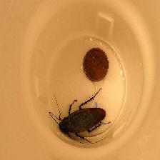
(a) Input Image: Cockroach

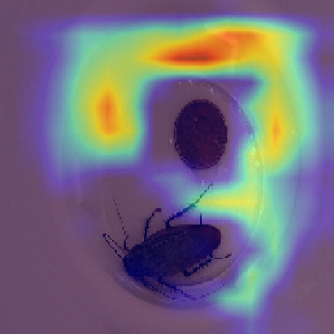
(b) VGG-16: Tick

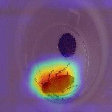
(c) Proposed: Cockroach

Figure 1: VGG-16 incorrectly classifies the input image, and the post hoc saliency map is inaccurate.The trustworthy CNN correctly classifies the image and produces an accurate saliency map.

2 Problem Setting

2.1 Prior Work

Consider a convolutional neural network $f$ that classifies an image $x_{i}$ into one of $c\in C$ classes. Let $y^{c}$ be the true label $c$ of an image $x_{i}$. Let $\hat{y}$ be $x_{i}$’s predicted label from $f$, or equivalently $\hat{y}=f(x_{i})_{c}$. The cross entropy is thus given by

$$CE(y,\hat{y})=\frac{1}{n}\sum\limits_{i=1}^{n}\sum\limits_{c=1}^{C}\mathds{-1}[y^{i}=c]\,log(f(x_{i})_{c})$$ (1)

Two saliency methods of particular interest are Grad-CAM and Guided Grad-CAM [31]. Let $A$ be the activation maps of some convolutional layer, a given activation map denoted $A^{k}$. To produce a saliency map for some $x_{i}$, Grad-CAM computes the gradients of the target class with respect to layer $l$’s activation maps. Global average pooling is performed on the gradients to serve as weights for each activation map. These weights, denoted $\alpha_{k}^{c}$ in equation 2 represent the importance of a given activation map $k$ for some target class $c\in C$.

$$\alpha_{k}^{c}=\frac{1}{W\times H}\sum\limits_{i}\sum\limits_{j}\frac{\partial y^{c}}{\partial A^{k}_{ij}}$$ (2)

After computing a weighted combination of the activation maps, the resulting output is passed through a ReLU. Here a ReLU is used to focus only on the features that have a positive influence on the true class $c$, i.e. pixels whose intensity should be increased in order to increase $y^{c}$ [31]. The saliency map output by Grad-CAM is thus given by

$$L^{c}_{(Grad-CAM)}=ReLU\left(\sum_{k}\alpha_{k}^{c}A^{k}\right)$$ (3)

Guided Grad-CAM [31] combines the output from Grad-CAM (equation 3) with the output from Guided Backpropagation [39] through element-wise multiplication. This is done for two reasons; First, Guided Backpropagation alone is not class discriminative. Second, Grad-CAM fails to produce high resolution (fine-grained) visualizations. Merging the two saliency methods produces saliency maps that are both high resolution and class discriminative [31].

2.2 Shortcomings

Despite state-of-the-art classification performance achieved by convolutional neural networks, loss minimizing parameters may result in saliency maps that do not highlight relevant pixels over the object of interest. Indeed the saliency map is dependent on the learned parameters. Parameters however are learned without knowing if the resulting saliency maps are visually accurate. Additionally, showing an inaccurate saliency map to a practitioner does not provide insight on how to change model parameters to correctly highlight pixels over the object of interest.

As an example, take a pre-trained model VGG-16 [36], trained on the ImageNet dataset [29]. We use Grad-CAM on selected images to identify relevant pixels. Figure 2 shows four different cases that can be encountered when using saliency methods for interpretations. Figure 2(b) shows the case $1$, where the predicted label is correct, and the resulting saliency map is visually accurate. Figure 2(g) shows case $2$, where the predicted class is incorrect, and the resulting saliency map is correct. Figure 2(l) shows case $3$, the predicted class is correct, and the resulting saliency map is inaccurate. Figure 2(q) shows case $4$, where the predicted class is incorrect and the resulting saliency map is inaccurate.

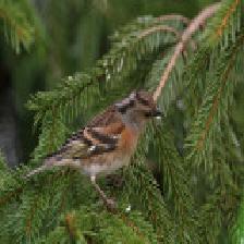
(a) True class:
Brambling

(b) Predicted class:
Brambling

(c) Predicted class:
Brambling

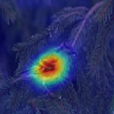
(d) Predicted class:
Brambling

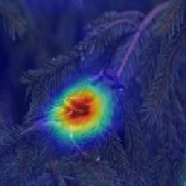
(e) Predicted class:
Brambling

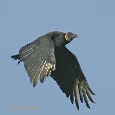
(f) True class:
Vulture

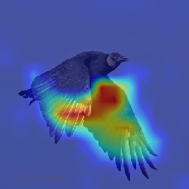
(g) Predicted class:
Kite

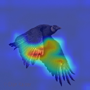
(h) Predicted class:
Vulture

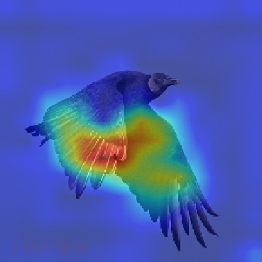
(i) Predicted class:
Vulture

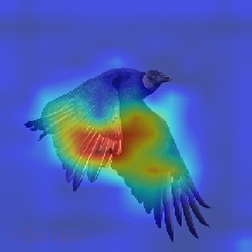
(j) Predicted class:
Vulture

(k) True class:
Pajama

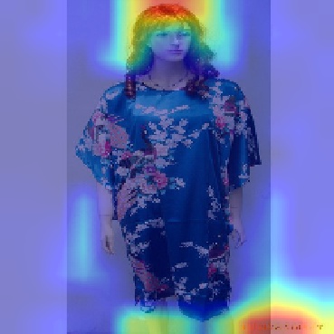
(l) Predicted class:
Pajama

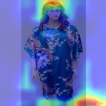
(m) Predicted class:
Pajama

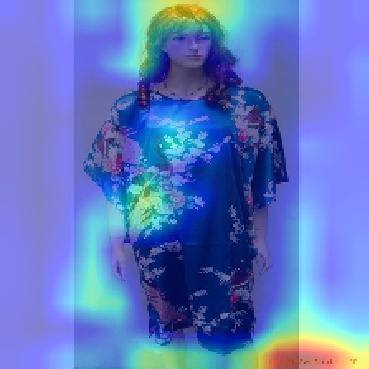
(n) Predicted class:
Pajama

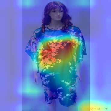
(o) Predicted class:
Pajama

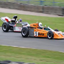
(p) True class:
Sports car

Input image

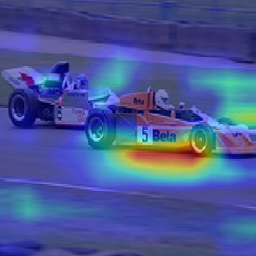
(q) Predicted class:
Racer

Baseline

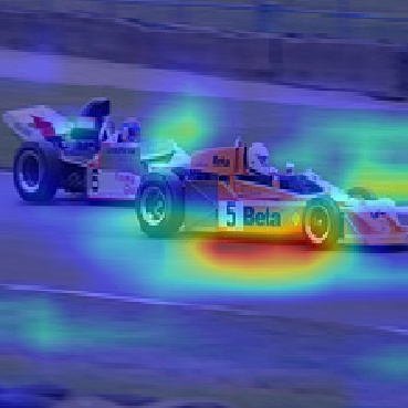
(r) Predicted class:
Sports car

Proposed ($.01$)

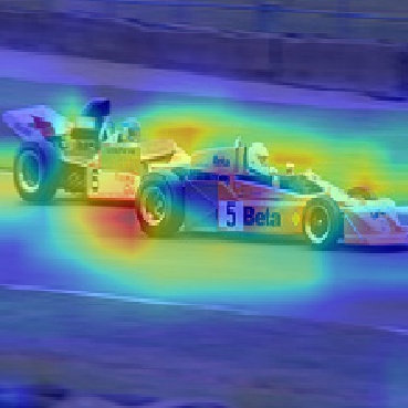
(s) Predicted class:
Sports car

Proposed ($.1$)

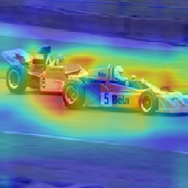
(t) Predicted class:
Sports car

Proposed ($.3$)

Figure 2: Input image shown with post hoc saliency maps from a VGG-16 baseline, and our proposed gradient penalized based Trustworthy CNN model shown with various learning rates.

Models giving inaccurate predictions (Figures 2(g), 2(q)) and/or inaccurate saliency maps (Figures 2(l), 2(q)) will cause users to lose trust in the model. Currently, convolutional neural networks are optimized ignoring how the saliency map will look post hoc. To our knowledge, no method exists to train convolutional neural networks to produce visually accurate saliency maps. We propose a loss function that penalizes inaccurate saliency maps, resulting in model parameters that produce visually accurate saliency maps post hoc, and improved classification performance, ensuring better user trust.

3 Trustworthy Convolutional Neural Networks

We define a trustworthy CNN as one that produces accurate predictions and visually accurate post hoc saliency maps determined by user evaluation.

3.1 Loss function

To identify parameters that produce both accurate predictions and accurate saliency maps, constraints must to be added to the cross entropy loss. Saliency maps produced post hoc can be visually accurate while the model classifies the observation incorrectly. Additionally, visually inaccurate saliency maps can be produced while the model classifies the observation correctly. Lastly, visually inaccurate saliency maps can be observed while the model incorrectly classifies the observation. The loss function must consider the saliency maps produced from the parameter choices at each step taken by the optimizer.

Take a saliency map $\hat{L}^{c}_{(.)_{i}}$ generated by a saliency method on the forward pass of training. We average the predicted saliency map across all dimensions. Given by equation 4, we use this penalty term to gauge the confidence of the predicted saliency map.

$$\hat{S}_{i}=\frac{1}{W\times H}\sum\limits_{w=1}^{W}\sum\limits_{h=1}^{H}\hat{L}^{c}_{(.)_{i}}$$ (4)

Adding the constraint of overly confident saliency maps generated during training does not penalize interactions between the saliency maps and predicted labels. Further constraints are needed to account for the predicted saliency map being accurate when the predicted label is incorrect, and the predicted saliency map being inaccurate when the predicted label is correct. Equation 5 and 6 are added for the interaction between the predicted class labels and predicted saliency map. Large gradient saliency maps with corresponding incorrect predicted labels are penalized, along with small gradient saliency maps with corresponding correct predicted labels.

$$R_{1}=CE(y_{i},\hat{y}_{i})(1-\hat{S}_{i})$$ (5)

$$R_{2}=\hat{S}_{i}(1-CE(y_{i},\hat{y}_{i}))$$ (6)

The final loss function used for all plots and tables in this work is given by equation 7. We use a scalar $\lambda\in[0,1]$ to establish a dependence between $\hat{S}_{i}$ and the cross entropy $CE$.

$$\mathcal{L}(y_{,}\hat{y},S)=\sum_{i=1}^{n}\lambda CE(y_{i},\hat{y}_{i})+(1-\lambda)S_{i}+R_{1}+R_{2}$$ (7)

The loss function we plan on using in future versions is given by

$$R_{1}=CE(y_{i},\hat{y}_{i})(1-PWCE(S_{i},\hat{S}_{i}))$$ (8)

$$R_{2}=PWCE(S_{i},\hat{S}_{i})(1-CE(y_{i},\hat{y}_{i}))$$ (9)

$$\mathcal{L}(y_{,}\hat{y},S,\hat{S})=\sum_{i=1}^{n}\lambda CE(y_{i},\hat{y}_{i})+(1-\lambda)PWCE(S_{i},\hat{S}_{i})+R_{1}+R_{2}$$ (10)

where $PWCE$ is the pixel-wise cross entropy between the ground truth saliency map and predicted saliency map.

3.2 Training

To optimize the loss proposed in equation 7, we freeze the weights of all other layers in the network. We use stochastic gradient descent in all our experiments, although any of its variants can be used.

Naturally, this loss function will be most effective in two settings; to update previously learned parameters of a pre-trained model, or learn parameters of a newly added layer in a transfer learning framework. Consider the following example, where a practitioner identifies a layer in a convolutional network that learns a noticeable systematic error. Our loss function allows practitioners to update the layer weights, and eliminate these errors without having to re-train the model from scratch. In the case of transfer learning, a new layer can be added and parameters can be learned that will produce accurate saliency maps post hoc.

There are no restrictions on which saliency method can be used to produce the saliency maps $L^{c}_{(.)_{i}}$ generated during training, provided the generated output when averaged is between zero and one. Regarding choice of saliency method, some choices make more intuitive sense than others. For example, Guided Backpropagation [39] and Deconvolutions [42] are not class discriminative, and therefore should not be chosen.

4 Experimental Studies

4.1 Transfer Learning

One interesting application of the proposed loss function is its application to the field of transfer learning [16]. Knowledge from models trained on a specific task are applied to an entirely different domain. Some recent developments [22, 15, 38, 10, 45], and several surveys [20, 46] can provide further detail.

We demonstrate how the proposed loss can be used in the context of transfer learning to improve classification performance. For this experiment, we use MobilenetV2 [30] on the cats and dogs dataset [9], found in Tensorflow [1]. The task is to classify whether an image contains a cat or dog, using the knowledge learned from the ImageNet dataset. We place one convolutional layer after the last convolutional layer in the MobilenetV2 network, closest to the softmax layer. This additional convolutional layer consists of $256$ filters, using a $1\times 1$ kernel with a stride of $1$. We then remove all layers after, and add a softmax layer. All other layer weights are frozen. The baseline model uses the cross entropy loss given by equation 1. We compare this against two trustworthy CNN models trained using equation 7. The first uses Grad-CAM to generate saliency maps during training, the second uses Guided Grad-CAM. We train all models for $50$ epochs using a batch size of $32$. We compare post hoc saliency maps using the structured similarity index (SSIM) given by equation 11, to compare relative to the baseline model. We fix the learning rate to $.01$ and set $\lambda=.9$.

$$SSIM(x,y)=\frac{(2\mu_{x}\mu_{y}+c_{1})(2\sigma_{xy}+c_{2})}{(\mu^{2}_{x}+\mu^{2}_{y}+c_{1})(\sigma^{2}_{x}+\sigma^{2}_{y}+c_{2})}$$ (11)

Where $c_{1}=(0.01L)^{2}$ and $c_{2}=(0.03L)^{2}$, and $L$ is defined by the dynamic range of the pixel values.

4.2 VGG-16 on ImageNet

As a second experiment, we apply our loss function to VGG-16 [36], trained on the ImageNet dataset [29] for an image classification task. Again we train two trustworthy models, one using Grad-CAM to generate saliency maps during training, the other using Guided Grad-CAM. We demonstrate improved post hoc saliency maps as evaluated by users, and improved classification performance. We compare this to a VGG-16 baseline trained using only the cross entropy loss. We use a subset of $30,000$ images, and update the parameters of VGG-16 from the $block5\_conv3$ layer. This layer was chosen as it is the closest convolutional layer to the softmax layer. We freeze the weights of all other layers. We compare classification performance of all models using accuracy, precision, and recall. We train different models varying the learning rate and lambda $\lambda$. We perform a grid search for the learning rate and lambda hyperparameters. We consider learning rates $\in\{.01,.1,.3\}$, and $\lambda\in\{.9,.7,.5\}$. Post hoc saliency maps are evaluated with a user experiment, detailed below.

4.2.1 User Experiment

To compare the post hoc saliency maps across models, a scoring metric is needed. Two commonly used metrics are localization error [31], or the pointing game [31, 43]. Both methods require ground truth object labels. We do not assume the data has any object annotations, hence these metrics cannot be used.

To score the post hoc saliency maps between the trustworthy gradient penalized models and their respective baselines, we conduct a user experiment. We take the best performing set of hyperparameters (learning rate of $.01$, and $\lambda=.9$), and use all models in the experiment to generate saliency maps for user evaluation.

We randomly sample test set images for user evaluation. We show users the input image and a post hoc saliency map from each model. We ask $29$ users "Which image best highlights the <true_class> in the original image." Users were given the option of "Can’t distinguish" and "They look the same" in the case that no saliency maps are convincing. Users are asked if they have a Bachelor’s degree in Computer Science, if they are familiar with the term saliency map used by the machine learning community, and if they have experience in computer vision. A link to the experiment can be found below. 

5 Results

5.1 Transfer Learning

The classification performance for all models can be found in Table 1. We observe the trustworthy MobilenetV2 model trained using Guided Grad-CAM outperformed the baseline and trustworthy Grad-CAM model. We find that both trustworthy CNN models outperformed their respective baseline models trained with just the cross entropy term.

The SSIM between saliency maps of the baseline model and trustworthy CNN trained with Grad-CAM was $.78$, and $.64$ between the baseline and trustworthy CNN trained with Guided Grad-CAM. When $R_{1}=0$, the SSIM for the trustworthy Grad-CAM and Guided Grad-CAM models drop to $.76$, and $.5$ respectively. When $R_{2}=0$, the SSIM for the trustworthy Grad-CAM and Guided Grad-CAM models increases to $.85$, and $.94$ respectively. This metric shows the post hoc saliency maps differ visually from the baseline, however, it fails to identify which saliency maps are more visually correct.

Table 1: Classification Performance-MobilenetV2

Model	Accuracy	Precision	Recall
MobilenetV2 Baseline	97.6%	97.6%	97.6%
Trustworthy CNN w/ Grad-CAM	98.4%	98.4%	98.4%
Trustworthy CNN w/ Grad-CAM ($R_{1}=0$)	98.3%	98.3%	98.3%
Trustworthy CNN w/ Grad-CAM ($R_{2}=0$)	98.5%	98.5%	98.5%
Trustworthy CNN w/ Guided Grad-CAM	98.7%	98.7%	98.7%
Trustworthy CNN w/ Guided Grad-CAM ($R_{1}=0$)	98.6%	98.6%	98.6%
Trustworthy CNN w/ Guided Grad-CAM ($R_{2}=0$)	98.4%	98.4%	98.4%

Classification performance on transfer learning task. $R_{1}=0$ denotes models trained with equation 5 set to zero, $R_{2}=0$ denotes models trained with equation 6.

Table 2: Classification Performance-VGG16

	Accuracy	Precision	Recall
VGG-16 Baseline	66% (56%,75%)	49.7%	50.8%
Trustworthy CNN w/ Grad-CAM	70% (61%, 78%)	54.6%	55.7%
VGG-16 Baseline	66% (56%,75%)	49.7%	50.8%
Trustworthy CNN w/ Guided Grad-CAM	70% (61%, 78%)	54.6%	55.7%

Classification performance shown for gradient penalized trustworthy models and baselines on test set images shown during user experiment. A $95\%$ confidence interval (lower, upper) is also included.

5.2 VGG-16 on ImageNet

Table 2 shows the accuracy, precision, and recall of all models on the subset of test set images shown to users in the experiment. We use the best performing set of hyperparameters to be evaluated by the users. We find that both trustworthy models outperform their respective baselines. We recognize the classification performance between the trustworthy models to be equal, likely due to setting $\lambda=.9$.

5.2.1 User Experiment

We find the SSIM between the baseline VGG-16 and trustworthy Grad-CAM model was $99.8$, and $99.4$ between the baseline VGG-16 and trustworthy Guided Grad-CAM model. According to this metric, the saliency maps generated by the gradient penalized models should be very similar to the base model. Through our user experiment however, we find this not to be the case. This is further discussed in Section 6.

Table 3 further breaks down the user experiment, showing the percentage of images that fall into each case. Users decided both trustworthy models outperform the baseline in all scenarios, except case $2$. Recall case $2$ occurs when the predicted label is incorrect and the saliency map is accurate. Ideally images fall into case $1$, and fewer images fall into cases $2$, $3$, and $4$.

Table 3: User Experiment Breakdown-VGG16

	Case $1$	Case $2$
VGG-16 Baseline	18% (7%,28%)	16% (6%, 26%)
Trustworthy CNN w/ Grad-CAM	44% (30%, 58%)	16% (6%, 26%)
VGG-16 Baseline	16% (6%, 26%)	10% (2%,18%)
Trustworthy CNN w/ Guided Grad-CAM	50% (36%, 64%)	18% (7%, 29%)
	Case $3$	Case $4$
VGG-16 Baseline	44% (30%, 58%)	16% (6%, 26%)
Trustworthy CNN w/ Grad-CAM	22% (10%, 33%)	12% (3%, 21%)
VGG-16 Baseline	48% (34%, 62%)	20% (9%,31%)
Trustworthy CNN w/ Guided Grad-CAM	18% (7%, 29%)	8% (0%, 20%)

For the Trustworthy CNN trained with Grad-CAM, $44\%$ of images shown to users were found to have accurate predictions, and more accurate saliency maps (relative to the baseline). A $95\%$ confidence interval (lower, upper) is included. Recall Case $1$: % of observations with predicted labels correct and resulting saliency maps accurate. Case $2$: % of observations with predicted labels incorrect and resulting saliency maps accurate. Case $3$: % of observations with predicted labels correct and resulting saliency maps inaccurate. Case $4$ % of observations with predicted labels incorrect and resulting saliency maps inaccurate. High percentage is desirable for Case $1$, low percentage is desirable for Cases $2$, $3$, and $4$.

5.3 Discussion

We find the trustworthy models trained with Guided Grad-CAM outperform all other models in terms of predicting correct labels and accurate post hoc saliency maps. In the transfer learning experiment, we find the SSIM decreases on gradient penalized models when equation 5 is set to zero. Additionally, the SSIM increases when equation 6 is set to zero. This shows the inherent trade-off between the two terms.

On the ImageNet dataset, users found the baseline VGG-16 models to produce inaccurate saliency maps. These models are not trustworthy. The most common error from the baseline models was producing accurate predictions with inaccurate saliency maps (case $3$ from Table 3). This is not surprising considering the cross entropy loss is saliency map unaware. Users will question the legitimacy of the model when inaccurate saliency maps are produced. Our approach offers improved classifiation results and more accurate saliency maps, resulting in increased user trust.

6 Limitations

6.1 Loss Function

One noticeable limitation using the proposed loss is that only one convolutional layer can be updated at a time in training. This is partially due to the limitations of some saliency methods. Grad-CAM and Guided Grad-CAM [31] for example generate saliency maps using the gradients from a specific layer only. Hence the gradients of one individual layer are used to compute the saliency map. This layer however may not fully represent what the entire model has learned.

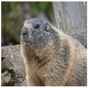
(a) Input Image

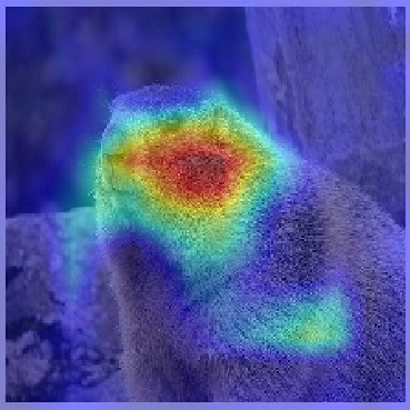
(b) Hypothetical Model 1

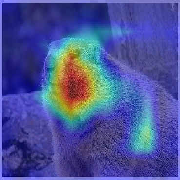
(c) Hypothetical Model 2

Figure 3: Two saliency maps with equal attribution values

6.2 Saliency Map Scoring

One difficulty in scoring saliency maps is that two saliency maps can correctly highlight the object of interest, but equal attribution values can be assigned to different parts of the same object. An example of this can be demonstrated in Figure 3 using two hypothetical models.

For some input image, both models output saliency maps with equal total attribution values, but pixels are attributed to different locations on the object. The model in Figure 3(b) attributes the face of the Marmot, and the model in Figure 3(c) attributes a portion of the face and body. These two saliency maps have exactly the same total attribution values when averaged. Hence, the SSIM between Figures 3(b) and 3(c) is $99.9$, but look significantly different. It is unclear which saliency map is more visually accurate.

7 Conclusion

In this work, we combine the use of post hoc interpretability methods with traditional loss functions to learn trustworthy model parameters. We propose a loss function that penalizes inaccurate saliency maps during training. Further constraining the loss function used by convolutional neural networks increases classification performance, and users found the post hoc saliency maps to be more accurate. This give a more dependable model. Future work involves extending this method to other tasks (image captioning, object tracking, etc), and other deep learning architectures.

Broader Impact

Users receiving an automated decision from a convolutional neural network will benefit from this research; Our approach provides a way to increase user trust in models previously treated as black box.

Using this approach, parameters of a pre-trained model can be updated, or parameters of a new layer can be learned in a transfer learning framework. Errors from an existing model can be identified and fixed. For practitioners wanting to eliminate a race or gender bias from a model, they will not have to retrain the model from scratch. This will save electricity used by the machine(s) to train.

We do not believe anyone is put at a disadvantage from this research. A failure of this system would mean the model would no longer be convincing to users, and thus no different than the original black box model.

References

- [1] Martín Abadi, Paul Barham, Jianmin Chen, Zhifeng Chen, Andy Davis, Jeffrey Dean, Matthieu Devin, Sanjay Ghemawat, Geoffrey Irving, Michael Isard, Manjunath Kudlur, Josh Levenberg, Rajat Monga, Sherry Moore, Derek Gordon Murray, Benoit Steiner, Paul A. Tucker, Vijay Vasudevan, Pete Warden, Martin Wicke, Yuan Yu, and Xiaoqiang Zheng. Tensorflow: A system for large-scale machine learning. In Kimberly Keeton and Timothy Roscoe, editors, 12th USENIX Symposium on Operating Systems Design and Implementation, OSDI 2016, Savannah, GA, USA, November 2-4, 2016, pages 265–283. USENIX Association, 2016.
- [2] Julius Adebayo, Justin Gilmer, Michael Muelly, Ian J. Goodfellow, Moritz Hardt, and Been Kim. Sanity checks for saliency maps. In Samy Bengio, Hanna M. Wallach, Hugo Larochelle, Kristen Grauman, Nicolò Cesa-Bianchi, and Roman Garnett, editors, Advances in Neural Information Processing Systems 31: Annual Conference on Neural Information Processing Systems 2018, NeurIPS 2018, 3-8 December 2018, Montréal, Canada, pages 9525–9536, 2018.
- [3] Marco Ancona, Enea Ceolini, Cengiz Öztireli, and Markus Gross. Towards better understanding of gradient-based attribution methods for deep neural networks. In 6th International Conference on Learning Representations, ICLR 2018, Vancouver, BC, Canada, April 30 - May 3, 2018, Conference Track Proceedings, 2018.
- [4] Stanislaw Antol, Aishwarya Agrawal, Jiasen Lu, Margaret Mitchell, Dhruv Batra, C. Lawrence Zitnick, and Devi Parikh. VQA: visual question answering. In 2015 IEEE International Conference on Computer Vision, ICCV 2015, Santiago, Chile, December 7-13, 2015, pages 2425–2433. IEEE Computer Society, 2015.
- [5] Rémi Cadène, Corentin Dancette, Hedi Ben-younes, Matthieu Cord, and Devi Parikh. Rubi: Reducing unimodal biases for visual question answering. In Wallach et al. [41], pages 839–850.
- [6] Chun-Hao Chang, Elliot Creager, Anna Goldenberg, and David Duvenaud. Explaining image classifiers by counterfactual generation. In 7th International Conference on Learning Representations, ICLR 2019, New Orleans, LA, USA, May 6-9, 2019. OpenReview.net, 2019.
- [7] Chaofan Chen, Oscar Li, Daniel Tao, Alina Barnett, Cynthia Rudin, and Jonathan Su. This looks like that: Deep learning for interpretable image recognition. In Wallach et al. [41], pages 8928–8939.
- [8] Ann-Kathrin Dombrowski, Maximilian Alber, Christopher J. Anders, Marcel Ackermann, Klaus-Robert Müller, and Pan Kessel. Explanations can be manipulated and geometry is to blame. In Wallach et al. [41], pages 13567–13578.
- [9] Jeremy Elson, John R. Douceur, Jon Howell, and Jared Saul. Asirra: a CAPTCHA that exploits interest-aligned manual image categorization. In Peng Ning, Sabrina De Capitani di Vimercati, and Paul F. Syverson, editors, Proceedings of the 2007 ACM Conference on Computer and Communications Security, CCS 2007, Alexandria, Virginia, USA, October 28-31, 2007, pages 366–374. ACM, 2007.
- [10] Steve Hanneke and Samory Kpotufe. On the value of target data in transfer learning. In Wallach et al. [41], pages 9867–9877.
- [11] Sara Hooker, Dumitru Erhan, Pieter-Jan Kindermans, and Been Kim. A benchmark for interpretability methods in deep neural networks. In Wallach et al. [41], pages 9734–9745.
- [12] Been Kim, Martin Wattenberg, Justin Gilmer, Carrie J. Cai, James Wexler, Fernanda B. Viégas, and Rory Sayres. Interpretability beyond feature attribution: Quantitative testing with concept activation vectors (TCAV). In Jennifer G. Dy and Andreas Krause, editors, Proceedings of the 35th International Conference on Machine Learning, ICML 2018, Stockholmsmässan, Stockholm, Sweden, July 10-15, 2018, volume 80 of Proceedings of Machine Learning Research, pages 2673–2682. PMLR, 2018.
- [13] Pieter-Jan Kindermans, Kristof T. Schütt, Maximilian Alber, Klaus-Robert Müller, Dumitru Erhan, Been Kim, and Sven Dähne. Learning how to explain neural networks: Patternnet and patternattribution. In 6th International Conference on Learning Representations, ICLR 2018, Vancouver, BC, Canada, April 30 - May 3, 2018, Conference Track Proceedings, 2018.
- [14] Alex Krizhevsky, Ilya Sutskever, and Geoffrey E. Hinton. Imagenet classification with deep convolutional neural networks. In Peter L. Bartlett, Fernando C. N. Pereira, Christopher J. C. Burges, Léon Bottou, and Kilian Q. Weinberger, editors, Advances in Neural Information Processing Systems 25: 26th Annual Conference on Neural Information Processing Systems 2012. Proceedings of a meeting held December 3-6, 2012, Lake Tahoe, Nevada, United States, pages 1106–1114, 2012.
- [15] Joshua Lee, Prasanna Sattigeri, and Gregory W. Wornell. Learning new tricks from old dogs: Multi-source transfer learning from pre-trained networks. In Wallach et al. [41], pages 4372–4382.
- [16] Fei-Fei Li, Robert Fergus, and Pietro Perona. One-shot learning of object categories. IEEE Trans. Pattern Anal. Mach. Intell., 28(4):594–611, 2006.
- [17] Scott M. Lundberg and Su-In Lee. A unified approach to interpreting model predictions. In Isabelle Guyon, Ulrike von Luxburg, Samy Bengio, Hanna M. Wallach, Rob Fergus, S. V. N. Vishwanathan, and Roman Garnett, editors, Advances in Neural Information Processing Systems 30: Annual Conference on Neural Information Processing Systems 2017, 4-9 December 2017, Long Beach, CA, USA, pages 4765–4774, 2017.
- [18] Grégoire Montavon, Sebastian Bach, Alexander Binder, Wojciech Samek, and Klaus-Robert Müller. Explaining nonlinear classification decisions with deep taylor decomposition. CoRR, abs/1512.02479, 2015.
- [19] Grégoire Montavon, Sebastian Lapuschkin, Alexander Binder, Wojciech Samek, and Klaus-Robert Müller. Explaining nonlinear classification decisions with deep taylor decomposition. Pattern Recognit., 65:211–222, 2017.
- [20] Sinno Jialin Pan and Qiang Yang. A survey on transfer learning. IEEE Trans. Knowl. Data Eng., 22(10):1345–1359, 2010.
- [21] Doina Precup and Yee Whye Teh, editors. Proceedings of the 34th International Conference on Machine Learning, ICML 2017, Sydney, NSW, Australia, 6-11 August 2017, volume 70 of Proceedings of Machine Learning Research. PMLR, 2017.
- [22] Maithra Raghu, Chiyuan Zhang, Jon M. Kleinberg, and Samy Bengio. Transfusion: Understanding transfer learning for medical imaging. In Wallach et al. [41], pages 3342–3352.
- [23] Joseph Redmon, Santosh Kumar Divvala, Ross B. Girshick, and Ali Farhadi. You only look once: Unified, real-time object detection. CoRR, abs/1506.02640, 2015.
- [24] Joseph Redmon and Ali Farhadi. YOLO9000: better, faster, stronger. In 2017 IEEE Conference on Computer Vision and Pattern Recognition, CVPR 2017, Honolulu, HI, USA, July 21-26, 2017, pages 6517–6525. IEEE Computer Society, 2017.
- [25] Joseph Redmon and Ali Farhadi. Yolov3: An incremental improvement. CoRR, abs/1804.02767, 2018.
- [26] Marco Túlio Ribeiro, Sameer Singh, and Carlos Guestrin. "why should I trust you?": Explaining the predictions of any classifier. In Balaji Krishnapuram, Mohak Shah, Alexander J. Smola, Charu C. Aggarwal, Dou Shen, and Rajeev Rastogi, editors, Proceedings of the 22nd ACM SIGKDD International Conference on Knowledge Discovery and Data Mining, San Francisco, CA, USA, August 13-17, 2016, pages 1135–1144. ACM, 2016.
- [27] Marco Túlio Ribeiro, Sameer Singh, and Carlos Guestrin. Anchors: High-precision model-agnostic explanations. In Sheila A. McIlraith and Kilian Q. Weinberger, editors, Proceedings of the Thirty-Second AAAI Conference on Artificial Intelligence, (AAAI-18), the 30th innovative Applications of Artificial Intelligence (IAAI-18), and the 8th AAAI Symposium on Educational Advances in Artificial Intelligence (EAAI-18), New Orleans, Louisiana, USA, February 2-7, 2018, pages 1527–1535. AAAI Press, 2018.
- [28] Laura Rieger, Chandan Singh, W. James Murdoch, and Bin Yu. Interpretations are useful: penalizing explanations to align neural networks with prior knowledge. CoRR, abs/1909.13584, 2019.
- [29] Olga Russakovsky, Jia Deng, Hao Su, Jonathan Krause, Sanjeev Satheesh, Sean Ma, Zhiheng Huang, Andrej Karpathy, Aditya Khosla, Michael S. Bernstein, Alexander C. Berg, and Fei-Fei Li. Imagenet large scale visual recognition challenge. Int. J. Comput. Vis., 115(3):211–252, 2015.
- [30] Mark Sandler, Andrew G. Howard, Menglong Zhu, Andrey Zhmoginov, and Liang-Chieh Chen. Mobilenetv2: Inverted residuals and linear bottlenecks. In 2018 IEEE Conference on Computer Vision and Pattern Recognition, CVPR 2018, Salt Lake City, UT, USA, June 18-22, 2018, pages 4510–4520. IEEE Computer Society, 2018.
- [31] Ramprasaath R. Selvaraju, Abhishek Das, Ramakrishna Vedantam, Michael Cogswell, Devi Parikh, and Dhruv Batra. Grad-cam: Why did you say that? visual explanations from deep networks via gradient-based localization. CoRR, abs/1610.02391, 2016.
- [32] Ramprasaath Ramasamy Selvaraju, Stefan Lee, Yilin Shen, Hongxia Jin, Shalini Ghosh, Larry P. Heck, Dhruv Batra, and Devi Parikh. Taking a HINT: leveraging explanations to make vision and language models more grounded. In 2019 IEEE/CVF International Conference on Computer Vision, ICCV 2019, Seoul, Korea (South), October 27 - November 2, 2019, pages 2591–2600. IEEE, 2019.
- [33] Avanti Shrikumar, Peyton Greenside, and Anshul Kundaje. Learning important features through propagating activation differences. In Precup and Teh [21], pages 3145–3153.
- [34] Avanti Shrikumar, Peyton Greenside, Anna Shcherbina, and Anshul Kundaje. Not just a black box: Learning important features through propagating activation differences. CoRR, abs/1605.01713, 2016.
- [35] Karen Simonyan, Andrea Vedaldi, and Andrew Zisserman. Deep inside convolutional networks: Visualising image classification models and saliency maps. In Yoshua Bengio and Yann LeCun, editors, 2nd International Conference on Learning Representations, ICLR 2014, Banff, AB, Canada, April 14-16, 2014, Workshop Track Proceedings, 2014.
- [36] Karen Simonyan and Andrew Zisserman. Very deep convolutional networks for large-scale image recognition. In Yoshua Bengio and Yann LeCun, editors, 3rd International Conference on Learning Representations, ICLR 2015, San Diego, CA, USA, May 7-9, 2015, Conference Track Proceedings, 2015.
- [37] Daniel Smilkov, Nikhil Thorat, Been Kim, Fernanda B. Viégas, and Martin Wattenberg. Smoothgrad: removing noise by adding noise. CoRR, abs/1706.03825, 2017.
- [38] Jie Song, Yixin Chen, Xinchao Wang, Chengchao Shen, and Mingli Song. Deep model transferability from attribution maps. In Wallach et al. [41], pages 6179–6189.
- [39] Jost Tobias Springenberg, Alexey Dosovitskiy, Thomas Brox, and Martin A. Riedmiller. Striving for simplicity: The all convolutional net. In Yoshua Bengio and Yann LeCun, editors, 3rd International Conference on Learning Representations, ICLR 2015, San Diego, CA, USA, May 7-9, 2015, Workshop Track Proceedings, 2015.
- [40] Mukund Sundararajan, Ankur Taly, and Qiqi Yan. Axiomatic attribution for deep networks. In Precup and Teh [21], pages 3319–3328.
- [41] Hanna M. Wallach, Hugo Larochelle, Alina Beygelzimer, Florence d’Alché-Buc, Emily B. Fox, and Roman Garnett, editors. Advances in Neural Information Processing Systems 32: Annual Conference on Neural Information Processing Systems 2019, NeurIPS 2019, 8-14 December 2019, Vancouver, BC, Canada, 2019.
- [42] Matthew D. Zeiler and Rob Fergus. Visualizing and understanding convolutional networks. In David J. Fleet, Tomás Pajdla, Bernt Schiele, and Tinne Tuytelaars, editors, Computer Vision - ECCV 2014 - 13th European Conference, Zurich, Switzerland, September 6-12, 2014, Proceedings, Part I, volume 8689 of Lecture Notes in Computer Science, pages 818–833. Springer, 2014.
- [43] Jianming Zhang, Zhe L. Lin, Jonathan Brandt, Xiaohui Shen, and Stan Sclaroff. Top-down neural attention by excitation backprop. In Bastian Leibe, Jiri Matas, Nicu Sebe, and Max Welling, editors, Computer Vision - ECCV 2016 - 14th European Conference, Amsterdam, The Netherlands, October 11-14, 2016, Proceedings, Part IV, volume 9908 of Lecture Notes in Computer Science, pages 543–559. Springer, 2016.
- [44] Bolei Zhou, Aditya Khosla, Àgata Lapedriza, Aude Oliva, and Antonio Torralba. Learning deep features for discriminative localization. In 2016 IEEE Conference on Computer Vision and Pattern Recognition, CVPR 2016, Las Vegas, NV, USA, June 27-30, 2016, pages 2921–2929. IEEE Computer Society, 2016.
- [45] Fuzhen Zhuang, Xiaohu Cheng, Ping Luo, Sinno Jialin Pan, and Qing He. Supervised representation learning: Transfer learning with deep autoencoders. In Qiang Yang and Michael J. Wooldridge, editors, Proceedings of the Twenty-Fourth International Joint Conference on Artificial Intelligence, IJCAI 2015, Buenos Aires, Argentina, July 25-31, 2015, pages 4119–4125. AAAI Press, 2015.
- [46] Fuzhen Zhuang, Zhiyuan Qi, Keyu Duan, Dongbo Xi, Yongchun Zhu, Hengshu Zhu, Hui Xiong, and Qing He. A comprehensive survey on transfer learning. CoRR, abs/1911.02685, 2019.
- [47] Luisa M. Zintgraf, Taco S. Cohen, Tameem Adel, and Max Welling. Visualizing deep neural network decisions: Prediction difference analysis. In 5th International Conference on Learning Representations, ICLR 2017, Toulon, France, April 24-26, 2017, Conference Track Proceedings. OpenReview.net, 2017.