Integrability of local and nonlocal non-commutative fourth order quintic nonlinear Schrödinger equations

Abstract.

We prove integrability of a generalised non-commutative fourth order quintic nonlinear Schrödinger equation. The proof is relatively succinct and rooted in the linearisation method pioneered by Ch. Pöppe. It is based on solving the corresponding linearised partial differential system to generate an evolutionary Hankel operator for the ‘scattering data’. The time-evolutionary solution to the non-commutative nonlinear partial differential system is then generated by solving a linear Fredholm equation which corresponds to the Marchenko equation. The integrability of reverse space-time and reverse time nonlocal versions, in the sense of Ablowitz and Musslimani [3], of the fourth order quintic nonlinear Schrödinger equation are proved contiguously by the approach adopted. Further, we implement a numerical integration scheme based on the analytical approach above which involves solving the linearised partial differential system followed by numerically solving the linear Fredholm equation to generate the solution at any given time.

1. Introduction

We prove that a generalised non-commutative fourth order quintic nonlinear Schrödinger equation is integrable. Here ‘integrable’ means the equation can be linearised. Precisely though briefly, given time-evolutionary solutions to the corresponding linearised equation, we can generate corresponding solutions to the original nonlinear equation at any given time by solving a linear integral Fredholm equation at that time. The Fredholm equation in question corresponds to the Marchenko equation. This approach to finding solutions to classical integrable systems such as the sine–Gordon, Korteweg de Vries, modified Korteweg de Vries, the whole associated Korteweg de Vries hierarchy and also the nonlinear Schrödinger equation was pioneered by Ch. Pöppe in a sequence of papers, see Pöppe [56, 57, 58], Pöppe and Sattinger [59] and Bauhardt and Pöppe [9]. Recently Doikou et al. [19, 18] extended Pöppe’s approach. First they demonstrated for the Korteweg de Vries and nonlinear Schrödinger equation, only Pöppe’s celebrated kernel product rule is required for the approach to work, see Doikou et al. [19]. Second they demonstrated the approach, as considered by Bauhardt and Pöppe [9], is naturally non-commutative and extends to the non-commutative nonlinear Schrödinger and non-commutative modified Korteweg de Vries equations, see Doikou et al. [18]. They also show how the method also naturally extends to nonlocal versions of these equations in the sense given in Ablowitz and Musslimani [3], i.e. where the nonlocality consists of reverse space-time or reverse time fields as factors in the nonlinear terms. The results herein extend the solution method developed in Doikou et al. [18], non-trivially, to the fourth order non-commutative case.

Let us explain Pöppe’s approach in some more detail. Consider a nonlinear complex matrix-valued partial differential equation for $g=g(x;t)$ of the form:

$$\partial_{t}g=d(\partial)g+\Psi(g,\partial g,\partial^{2}g,\ldots),$$

where $\partial=\partial_{x}$. Here we suppose $d=d(\partial)$ is a constant coefficient polynomial in $\partial$, while $\Psi$ is a precise homogeneous non-commutative polynomial function of $g$ and its partial derivatives up to an order two less than the degree of $d$. Without loss of generality we assume we have subsumed any homogeneous linear terms in $\Psi$ into the term $d(\partial)g$. Hence $\Psi$ encodes all the nonlinear terms in the partial differential equation shown. Setting $\Psi=O$, the zero matrix, consider the corresponding linear partial differential equation for the complex matrix-valued function $p=p(x;t)$ as follows:

$$\partial_{t}p=d(\partial)p.$$

The quantity $p=p(x;t)$ represents the ‘scattering data’. The first step in Pöppe’s approach is to elevate the Marchenko equation to the operator level. We construct a Hankel operator $P=P(x,t)$ associated with the scattering data as follows. We assume $P$ is a Hilbert–Schmidt operator with integral kernel given by $p=p(y+z+x;t)$ so that for any square-integrable function $\phi$:

$$(P\phi)(y;x,t)\coloneqq\int_{-\infty}^{0}p(y+z+x;t)\phi(z)\,\mathrm{d}z.$$

Note that $P=P(x,t)$ satisfies the operator differential equation $\partial_{t}P=d(\partial)P$. We then define an associated ‘data’ operator $Q=Q(x,t)$ by $Q\coloneqq P^{\dagger}P$, where $P^{\dagger}$ is the adjoint operator to $P$. This precise assignment for $Q$ does depend on the application at hand. For the applications herein we make the choice stated, guided by Ablowitz et al. [6]. The crucial classical ingredient is the Marchenko equation and here, at the operator level, this has the form:

$$P=G({\mathrm{id}}+Q).$$

This is a linear Fredholm equation for the operator $G=G(x,t)$. Hence to recap, the three key ingredients in the first step in Pöppe’s approach are the: (i) Operator differential equation for $P=P(x,t)$; (ii) Assignment for the auxiliary data operator $Q=Q(x,t)$ and (iii) Linear Fredholm equation for $G=G(x,t)$.

The second step in Pöppe’s approach, and the major underlying insight, is the ‘kernel product rule’, in which the Hankel property of $P$ plays a crucial role. Suppose $F=F(x,t)$ is a Hilbert–Schmidt linear operator with kernel $f(y,z;x,t)$. Note we assume $f$ depends on the parameters $x$ and $t$. For example recall from above $P=P(x,t)$ is a Hankel operator with kernel $p=p(y+z+x;t)$. Let us denote by $[F]$ the kernel of $F$, i.e. $[F]=f$. Now suppose $F=F(x,t)$ and $F^{\prime}=F^{\prime}(x,t)$ are Hilbert–Schmidt operators with kernels continuous in $x$. In addition suppose $H$ and $H^{\prime}$ are Hilbert–Schmidt Hankel operators with kernels continuously differentiable in $x$. Then the fundamental theorem of calculus implies

$$\bigl{[}F\partial_{x}(HH^{\prime})F^{\prime}\bigr{]}(y,z;x,t)=[FH](y,0;x,t)[H^{\prime}F^{\prime}](0,z;x,t).$$

This is the crucial ‘kernel product rule’ composing the second step in Pöppe’s approach. More precisely, Pöppe used the ‘trace’ form of this rule evaluated at $y=z=0$. We prefer to delay this specialisation until the final step in the procedure. The kernel product rule is the only property we use in Doikou et al. [19, 18] and herein.

The third and final step is to compute $\partial_{t}G-d(\partial)G$ where from the linear Fredholm equation above $G=PU$ with $U\coloneqq({\mathrm{id}}+Q)^{-1}$. And we then apply the kernel bracket operator $[\,\cdot\,]$. The basic calculus property $\partial U=-U(\partial Q)U$ initiates the generation of nonlinear terms. The goal is then to use only the kernel product rule to establish a ‘closed form’ for the nonlinear terms generated. By a ‘closed form’ we mean the terms generated represent a constant coefficient non-commutative polynomial in $[G]$, $\partial[G]$, $\partial^{2}[G]$ and so forth. Hence for example, if $d(\partial)=\mu_{4}\partial^{4}$ and $\mu_{4}$ is a pure imaginary constant parameter then in our main Theorem 3.1 we show if $P=P(x,t)$ satisfies $\partial_{t}P=d(\partial)P$ and $Q=P^{\dagger}P$, then $[G]$ satisfies the non-commutative nonlinear partial differential equation,

$$\partial_{t}[G]-\mu_{4}\partial^{4}[G]= \;2\mu_{4}\Bigl{(}2\bigl{(}\partial^{2}[G]\bigr{)}[G]^{\dagger}[G]+[G]\bigl{(}\partial^{2}[G]^{\dagger}\bigr{)}[G]+2[G][G]^{\dagger}\bigl{(}\partial^{2}[G]\bigr{)}$$

$$\;+\bigl{(}\partial[G]\bigr{)}\bigl{(}\partial[G]^{\dagger}\bigr{)}[G]+3\bigl{(}\partial[G]\bigr{)}[G]^{\dagger}\bigl{(}\partial[G]\bigr{)}+[G]\bigl{(}\partial[G]^{\dagger}\bigr{)}\bigl{(}\partial[G]\bigr{)}$$

$$\;+3[G][G]^{\dagger}[G][G]^{\dagger}[G]\Bigr{)}.$$

In the above, $P^{\dagger}$ is the operator adjoint to $P$ while $[G]^{\dagger}$ is the kernel function corresponding to the complex-conjugate transpose of the kernel function $[G]$. In the formulation above we have suppressed the parameter dependence of both the kernels $[G]=[G](y,z;x,t)$ and the kernels of the nonlinear terms—recall the kernel product rule above. Hence for example two applications of the kernel product rule led to the first term on the right which in full should read

$$4\mu_{4}\bigl{(}\partial^{2}[G](y,0;x,t)\bigr{)}[G]^{\dagger}(0,0;x,t)[G](0,z;x,t),$$

and so forth for the other cubic terms. Four applications of the kernel product rule generated the quintic term whose left and right factors should have parameter dependencies matching those of the corresponding factors in the cubic term above, and whose three central factors should have the parameter dependence $(0,0;x,t)$. By a standard convention we invoke, these dependencies are implied in the non-commutative equation above. We now emphasise that we can set $y=z=0$ throughout so that all the terms have the parameter dependence $(0,0;x,t)$. This generates the non-commutative fourth order quintic nonlinear Schrödinger equation. Furthermore the solution to this equation is generated as follows. We solve the linear partial differential equation, namely $\partial_{t}p=\mu_{4}\partial^{4}p$. This can be achieved analytically. The solution function $p$ generates the kernel of the Hankel operator $P=P(x,t)$. We set $Q=P^{\dagger}P$, this involves computing an integral whose integrand is a known function. We can then compute the solution to the non-commutative fourth order quintic nonlinear Schrödinger equation for $[G]=[G](y,z;x,t)$ shown above by solving the linear Fredholm equation $P=G({\mathrm{id}}+Q)$ for $G$. Hence the quintic nonlinear Schrödinger above is linearsiable and thus integrable in this sense.

As another example, consider the case of a non-commutative fourth order quintic nonlinear Schrödinger equation with a nonlocal nonlinearity as follows. Suppose the Hankel operator $P=P(x,t)$ satisfies the same partial differential equation $\partial_{t}P=\mu_{4}\partial^{4}P$ as in the example just above with $\mu_{4}$ a pure imaginary constant parameter. However, we now specify that $Q=\tilde{P}P$ where the operator $\tilde{P}=\tilde{P}(x,t)$ is given by $\tilde{P}(x,t)=P^{\mathrm{T}}(-x,-t)$, where $P^{\mathrm{T}}$ is the operator whose matrix kernel is the transpose of the matrix kernel corresponding to $P$. Then $[G]$ satisfies an analogous non-commutative nonlinear partial differential equation to that shown above, except that the terms $[G]^{\dagger}$ on the right-hand side are replaced by $[\tilde{G}]$ where $\tilde{G}=\tilde{G}(x,t)$ is given by $\tilde{G}(x,t)=G^{\mathrm{T}}(-x,-t)$. As in the last example, $[G]=[G](y,z;x,t)$, and we can set $y=z=0$ throughout so that all the terms have the parameter dependence $(0,0;x,t)$. This generates the reverse space-time nonlocal non-commutative fourth order quintic nonlinear Schrödinger equation; see Example 3.3 in the main text. The solution to this equation can be generated in an analogous manner to that described in the example just above, demonstrating the equation is linearisable and thus integrable.

In Doikou et al. [19] with $d(\partial)=\mu_{2}\partial^{2}$ and $\mu_{2}$ a constant pure imaginary parameter, we generated the solution to the nonlinear Schrödinger equation in this way. With $d(\partial)=\mu_{3}\partial^{3}$ and $\mu_{3}$ a real parameter, and a slight modification of the procedure above, we generated solutions to the Korteweg de Vries equation. Then in Doikou et al. [18] we generalised this approach to the non-commutative setting and also generated solutions to the non-commutative modified Korteweg de Vries in this way from $d(\partial)=\mu_{3}\partial^{3}$. Note, with the solution procedure described above, the specific choices of $d=d(\partial)$ indicated, generate precise non-commutative polynomial functions $\Psi$ representing the nonlinear terms. In preceding work, Beck et al. [11, 12] assume the kernels $p=p(y,z;t)$ and $q=q(y,z;t)$ associated with the operators $P$ and $Q$ satisfy a coupled pair of linear partial differential equations. They show the kernel $[G]=[G](y,z;t)$ associated with the operator $G$ solving the linear Fredholm equation $P=G({\mathrm{id}}+Q)$ satisfies a Riccati partial differential equation which can be interpreted as a nonlocal nonlinear partial differential equation. For example Beck et al. [12] generate solutions to the following nonlocal Korteweg de Vries equation for $[G]=[G](y,z;t)$ using this approach:

$$\partial_{t}[G](y,z;t)-\partial^{3}_{y}[G](y,z;t)=\int_{{\mathbb{R}}}[G](y,\xi;t)\bigl{(}\partial_{\xi}[G](\xi,z;t)\bigr{)}\,{\mathrm{d}}\xi.$$

The nonlocal nonlinearity is the realisation at the kernel level of a linear operator product, and the kernel product rule is not used. All the nonlinear flows in Beck et al. [11, 12] and Doikou et al. [19, 18] are shown to be Grassmannian flows. Indeed the theory in Doikou et al. [18, Section 2.3] establishes the flow generated in our main Theorem 3.1 is also a Grassmannian flow.

In actuality, we consider an inflated coupled linear system, one which includes the linear partial differential equation $\partial_{t}P=d(\partial)P$ for $P=P(x,t)$, but more generally assigns $Q\coloneqq\tilde{P}P$ where $\tilde{P}=\tilde{P}(x,t)$ is a linear operator analogous to $P$ satisfying an associated linear partial differential equation $\partial_{t}\tilde{P}=\tilde{d}(\partial)\tilde{P}$. Here $\tilde{d}=\tilde{d}(\partial)$ is a constant coefficient polynomial in $\partial$ analogous to $d(\partial)$, of the same degree. We correspondingly assign $\tilde{Q}\coloneqq P\tilde{P}$. And finally in addition to $P=G({\mathrm{id}}+Q)$ we now include the analogous linear Fredholm equation $\tilde{P}=\tilde{G}({\mathrm{id}}+\tilde{Q})$. See Definition 2.7 for the inflated linear system. The inflated system also naturally generates a Grassmannian flow; see Doikou et al. [18]. Naturally we must assume the complex matrix-valued kernels of $P$ and $\tilde{P}$ are commensurate so that $Q$ and $\tilde{Q}$ make sense. Consequently with suitable restrictions on $\tilde{d}(\partial)$ we can choose $\tilde{P}=P^{\dagger}$ as above. Or for example, we can also consistently choose $\tilde{P}(x,t)=P^{\mathrm{T}}(-x,-t)$ where $P^{\mathrm{T}}$ is the linear operator whose kernel is the transpose of the kernel for $P$. In this case $\tilde{G}(x,t)=G^{\mathrm{T}}(-x,-t)$ and we generate a non-commutative quintic equation like that above with $[G]^{\dagger}$ replaced by $G^{\mathrm{T}}(-x,-t)$ everywhere. Thus the corresponding reverse space-time nonlocal non-commutative quintic equation, in the sense of Ablowitz and Musslimani [3], is linearisable.

We also develop a numerical method for solving such integrable systems, first explored in Doikou et al. [19]. The numerical method applies to any of the integrable systems such as the non-commutative nonlinear Schrödinger and modified Korteweg de Vries equations considered in Doikou et al. [18], as well as the non-commutative fourth order quintic equation above, or indeed, the more general non-commutative fourth order quintic equation which we establish is linearisable and integrable as our main result in Theorem 3.1. We can analytically solve the linearised partial differential system for the Hankel operator $P=P(x,t)$ or indeed its corresponding kernel $p=p(x,t)$, in Fourier space. This is because $p$ satisfies the linear partial differential equation $\partial_{t}=d(\partial)p$, where $d(\partial)$ is a constant coefficient polynomial in $\partial$. Hence in principle we can evaluate $p=p(x,t)$ at any given time $t>0$, or in practice we can represent it to any degree of accuracy determined by the finite number of Fourier modes we choose to represent the Fourier series of $p=p(x,t)$, on a truncated domain. We can then determine the kernel function $q=q(y,z;x,t)$ corresponding to the associated data operator $Q=Q(x,t)$ by evaluating $Q=P^{\dagger}P$ by computing,

$$q(y,z;x,t)=\int_{-\infty}^{0}p^{\dagger}(y+\zeta+x;t)p(\zeta+z+x;t)\,{\mathrm{d}}\zeta.$$

Note $P^{\dagger}$ denotes the adjoint operator to $P$, while for the kernel function $p^{\dagger}$ denotes the complex conjugate transpose to the complex matrix-valued function $p$. Using our representation for $p$ we can approximate the integral on the right-hand side to compute an approximation for $q$. To compute the operator $G$ we need to solve the Fredholm equation $P=G({\mathrm{id}}+Q)$, i.e. if $g=g(y,z;x,t)$ is the kernel corresponding to $G$, we numerically solve the Fredholm integral equation

$$p(y+z+x;t)=g(y,z;x,t)+\int_{-\infty}^{0}g(y,\zeta;x,t)q(\zeta,z;x,t\,{\mathrm{d}}\zeta.$$

We achieve this by approximating the integral on the right-hand side by a Riemann sum and solving the resulting large linear algebraic system of equations. We then set $y=z=0$ to determine $g(0,0;x,t)$, the kernel correspondng to $[G](0,0;x,t)$. The method works for any given initial data function $p_{0}=p_{0}(x)$ for which $p(x,0)=p_{0}(x)$. In principle, given any initial data function $g_{0}=g_{0}(x)$ for which $g(0,0;x,0)=g_{0}(x)$ we could compute $p(x,0)$ via ‘scattering’ methods, however we do not implement this here. In general the overall numerical procedure we implement is straightforward, and in practice, appears to be robust.

In addition to the series of papers by Pöppe mentioned above, the work herein was also motiviated by Ablowitz et al. [6], Dyson [20] and McKean [48]. We also mention in this context Ercolani and McKean [23] and Mumford [50, p. 3.239]. The Marchenko equation is central not only to Pöppe’s approach, but also to that of Fokas and Ablowitz [26], Nijhoff et al. [52] and the Zakharov–Shabat scheme [72, 73]. Details of Fokas’ unified transform method can be found for example in Fokas and Pelloni [27]. Hankel operators have received a lot of recent attention, see Grudsky and Rybkin [32, 33], Grellier and Gerard [31] and Blower and Newsham [14]. Nonlocal integrable systems have also received a lot of recent attention, see Ablowitz and Musslimani [3], Fokas [25], Grahovski, Mohammed and Susanto [30] and Gürses and Pekcan [36, 37, 38, 39]. The scalar reverse time nonlocal nonlinear Schrödinger equation is $PT$ symmetric, and was derived in Ablowitz and Musslimani [2] “with physical intuition”. Indeed, Ablowitz and Musslimani [4] establish “an important physical connection between the recently discovered nonlocal integrable reductions of the AKNS system and physically interesting equations”. Further, quoting from Gerdjikov and Saxena [29], “nonlocal, nonlinear equations arise in a variety of physical contexts ranging from hydrodynamics to optics to condensed matter and high energy physics”. See Lou and Huang [44] for a derivation of the nonlocal ‘Alice–Bob Korteweg de Vries’ system from a system of equations modelling atmospheric dynamics. A local non-commutative fourth order quintic nonlinear Schrödinger equation corresponding to that above can be found in Nijhoff et al. [52, eq. B.4a] who establish integrability via the method pioneered by Fokas and Ablowitz [26]. Indeed Nijhoff et al. [52, eq. B.5a] also present the non-commutative fifth order quintic nonlinear Schrödinger equation. For further early work on non-commutative integrable systems, see in addition, Manakov [46], Fordy and Kulisch [28] and Ablowitz et al. [5]. For more recent work on the multi-component nonlinear Schrödinger equation, as well as its discretisation, see Ablowitz et al. [5], Degasperis and Lombardo [16] and Pelinovksy [55]. We remark we do not utilise a Lax pair $L\upsilon=\lambda\upsilon$ and $\partial_{t}\upsilon=D\upsilon$ for the auxiliary function $\upsilon$ and spectral parameter $\lambda$, and require compatability. Here we use the linearised evolution equation $\partial_{t}\upsilon=D\upsilon$ and require $\upsilon$ to have the Hankel property.

General higher order nonlinear Schrödinger equations have recently received a lot of attention; see Karpman [41], Karpman and Shagalov [42], Ben–Artzi et al. [13], Fibich et al. [24], Pausader [54], Boulenger and Lenzmann [15], Kwak [43], Oh and Wang [53] and Posukhovskyi and Stefanov [60]. More specifically though, in our main result in Theorem 3.1 we establish integrability for a more general system of equations than that shown for $[G]$ above. The more general system also includes standard nonlinear Schrödinger dispersion and nonlinear terms, both with the scalar constant pure imaginary factor $\mu_{2}$, as well as the next order terms in the nonlinear Schrödinger hierarchy, namely standard non-commutative modified Korteweg de Vries third order dispersion and nonlinear terms, both with the scalar constant real factor $\mu_{3}$. The commutative form of this more general equation, involving the parameters $\mu_{2}$, $\mu_{3}$ and $\mu_{4}$ have recently found applications as models for short pulse propagation in optical fibres as follows; see Kang et al. [40] and Agrawal [7]. The fundamental nonlinear Schrödinger equation itself, corresponding to $\mu_{3}=\mu_{4}=0$ describes the propagation of picosecond pulses in an optical fibre. The case when $\mu_{4}=0$ (only) corresponds to the Hirota equation which describes the propagation of femtosecond soliton pulses in the mono-mode optical fibres, see Demiray et al. [17], Mihalache et al. [49] and Nakkeeran [51]. The case when with $\mu_{2}$ and $\mu_{4}$ pure imaginary, and $\mu_{3}$ real, with all three non-zero describes “ultrashort optical-pulse propagation in a long-distance, high-speed optical fibre transmission system”, see again Kang et al. [40] or Guo et al. [35]. Also see Wang et al. [70] who consider the case $\mu_{3}=0$ (only). Attosecond pulses in an optical fibre are described by a fifth order nonlinear Schrödinger equation. Indeed Kang et al. [40] consider and eighth order nonlinear Schrödinger equation as a model for ultrashort pulse propagation. The nonlinear Schrödinger hierarchy up to and including order eight can be found in Matveev and Smirnov [47] who consider multi-rogue wave solutions. For applications to pulses in erbium-doped fibres modelled by the higher order nonlinear Schrödinger equations above coupled to a Maxwell–Bloch system, see Guan et al. [34], Guo et al. [35], Ren et al. [62], Wang et al. [68], Wang et al. [69] and Wang et al. [71].

To summarise, what is new in this paper is we:

1. Give a direct proof, based on the Hankel operator approach of Ch. Pöppe, that a generalised non-commutative fourth order quintic nonlinear Schrö-dinger equation is linearisable and thus integrable (Theorem 3.1);

2. Prove reverse space-time and reverse time nonlocal versions, in the sense of Ablowitz and Musslimani [3], of the non-commutative fourth order quintic nonlinear Schrödinger equation, are also linearisable and thus integrable. These results are specialisations of the approach utilised to establish (i);

3. Develop a numerical method to accurately evaluate the solution to such integrable systems at any given time, based on the analytical linearisation approach in (i). The numerical method involves the analytical solution of the linearised partial differential system at the time given, computing an associated data function and then numerically solving a linear Fredholm equation to generate the solution at that time. The method is straightforward, and in practice appears to be robust.

Our paper is organised as follows. In Section 2 we introduce the notation and key concepts and identities we need to prove our main result. The latter is presented and proved in Section 3. We demonstrate our numerical method based on the analytical approach above in Section 4. We include some insights on, and comments on future directions for, the work herein in the final Discussion Section 5.

2. Preliminaries

We consider Hilbert–Schmidt integral operators which depend on both a spatial parameter $x\in\mathbb{R}$ and a time parameter $t\in[0,\infty)$. Throughout $\partial_{t}$ represents the partial derivative with respect to the time parameter $t$ while $\partial=\partial_{x}$ represents the partial derivative with respect to the spatial parameter $x$. Hilbert–Schmidt operators are representable in terms of square-integrable kernels. Hence for a given Hilbert–Schmidt operator $F=F(x,t)$, there exists a square-integrable kernel $f=f(y,z;x,t)$ such that for any square-integrable function $\phi$,

$$(F\phi)(y;x,t)=\int_{-\infty}^{0}f(y,z;x,t)\phi(z)\,\mathrm{d}z.$$

Definition 2.1 (Kernel bracket).

With reference to the operator $F$ just above, we use the kernel bracket notation $[F]$ to denote the kernel of $F$:

$$[F](y,z;x,t)\coloneqq f(y,z;x,t).$$

We often drop the dependencies and simply write $[\,\cdot\,]$.

Of critical importance throughout this paper is a class of integral operators known as Hankel operators. We consider Hankel operators which depend on a parameter $x$ as follows.

Definition 2.2 (Hankel operator with parameter).

We say a given time-dependent Hilbert–Schmidt operator $H$ with corresponding square-integrable kernel $h$ is Hankel or additive with parameter $x\in{\mathbb{R}}$ if its action, for any square-integrable function $\phi$, is given by

$$(H\phi)(y;x,t)\coloneqq\int_{-\infty}^{0}h(y+z+x;t)\phi(z)\,\mathrm{d}z.$$

Hankel operators of this form are the starting point for Pöppe’s approach; see Pöppe [56, 57] and Doikou et al. [19, 18]. As mentioned in the introduction there is a crucial kernel product rule we rely on throughout. This is as follows. We include the proof from Doikou et al. [19, 18] for completeness.

Lemma 2.3 (Kernel product rule).

Assume $H,H^{\prime}$ are Hilbert–Schmidt Hankel operators with parameter $x$ and $F,F^{\prime}$ are Hilbert–Schmidt operators. Assume further that the corresponding kernels of $F$ and $F^{\prime}$ are continuous and of $H$ and $H^{\prime}$ are continuously differentiable. Then, the following kernel product rule holds,

$$[F\partial(HH^{\prime})F^{\prime}](y,z;x)=[FH](y,0;x)[H^{\prime}F^{\prime}](0,z;x).$$

Proof.

We use the fundamental theorem of calculus and Hankel properties of $H$ and $H^{\prime}$. Let $f$, $h$, $h^{\prime}$ and $f^{\prime}$ denote the integral kernels of $F$, $H$, $H^{\prime}$ and $F^{\prime}$ respectively. By direct computation $[F\partial_{x}(HH^{\prime})F^{\prime}](y,z;x)$ equals

$$\int_{{\mathbb{R}}_{-}^{3}}f(y,\xi_{1};x)\partial_{x}\bigl{(}h(\xi_{1}+\xi_{2}+x)h^{\prime}(\xi_{2}+\xi_{3}+x)\bigr{)}f^{\prime}(\xi_{3},z;x)\,{\mathrm{d}}\xi_{3}\,{\mathrm{d}}\xi_{2}\,{\mathrm{d}}\xi_{1}$$

$$=\int_{{\mathbb{R}}_{-}^{3}}f(y,\xi_{1};x)\partial_{\xi_{2}}\bigl{(}h(\xi_{1}+\xi_{2}+x)h^{\prime}(\xi_{2}+\xi_{3}+x)\bigr{)}f^{\prime}(\xi_{3},z;x)\,{\mathrm{d}}\xi_{3}\,{\mathrm{d}}\xi_{2}\,{\mathrm{d}}\xi_{1}$$

$$=\int_{{\mathbb{R}}_{-}^{2}}f(y,\xi_{1};x)h(\xi_{1}+x)h^{\prime}(\xi_{3}+x)f^{\prime}(\xi_{3},z;x)\,{\mathrm{d}}\xi_{3}\,{\mathrm{d}}\xi_{1}$$

$$=\int_{{\mathbb{R}}_{-}}f(y,\xi_{1};x)h(\xi_{1}+x)\,{\mathrm{d}}\xi_{1}\cdot\int_{{\mathbb{R}}_{-}}h^{\prime}(\xi_{3}+x)f^{\prime}(\xi_{3},z;x)\,{\mathrm{d}}\xi_{3}$$

$$=\bigl{(}[FH](y,0;x)\bigr{)}\bigl{(}[H^{\prime}F^{\prime}](0,z;x)\bigr{)},$$

giving the result. ∎

This kernel bracket operator and product rule above originates from the work of Pöppe in [56, 57, 58] and Bauhardt and Pöppe [9]. We record in the following lemma some identities for $W\coloneqq(\mathrm{id}+F)^{-1}$ which are useful later on. We assume $F$ depends on a parameter. Similar results are derived by Pöppe [56, 57].

Lemma 2.4 (Inverse operator identities).

Suppose the operator $F$ depends on a parameter with respect to which we wish to compute derivatives. Further suppose $W\coloneqq(\mathrm{id}+F)^{-1}$ exists. Then the following identities hold:

1. ${\mathrm{id}}-W=WF=FW$;

2. $\partial W=-W(\partial F)W$;

3. $\partial W=-(\partial W)F-W(\partial F)=-(\partial F)W-F(\partial W)$;

4. $\partial^{2}W=-2(\partial W)(\partial F)W-W(\partial^{2}F)W$;

5. $\partial^{3}W=-3(\partial^{2}W)(\partial F)W-3(\partial W)(\partial^{2}F)W-W(\partial^{3}F)W$;

6. $\partial^{4}W=-4(\partial^{3}W)(\partial F)W-6(\partial^{2}W)(\partial^{2}F)W-4(\partial W)(\partial^{3}F)W-W(\partial^{4}F)W$.

Proof.

The first identity is straightforward. The others follow by successively differentiating ${\mathrm{id}}-W=WF$ and finally using $W\coloneqq({\mathrm{id}}+Q)^{-1}$ in each form. ∎

We have the following corollary to Lemma 2.4, which can also be found in Doikou et al. [18].

Corollary 2.5.

Suppose we set $F\coloneqq Q$ with $Q=\tilde{P}P$ and $U\coloneqq(\mathrm{id}+Q)^{-1}$ so $U=(\mathrm{id}+\tilde{P}P)^{-1}$. Assume $U$ exists. Then $U$ satisfies properties (i)–(vi) in Lemma 2.4. Further suppose we set $F\coloneqq\tilde{Q}$ with $\tilde{Q}=P\tilde{P}$ and $V\coloneqq(\mathrm{id}+\tilde{Q})^{-1}$. Assume $V$ exists. Then similarly $V$ satisfies properties (i)–(vi) in Lemma 2.4. We note $PU^{-1}=V^{-1}P$, so we have $VP=PU$. Similarly, we have $U\tilde{P}=\tilde{P}V$.

The following key identities also prove useful throughout the proof of our main result in Section 3. To keep our statements succinct hereafter we use the following notation convention. For the kernel product rule introduced in Lemma 2.3, for the terms on the right we simply write $[FH][H^{\prime}F^{\prime}]$, where it is understood the left factor is evaluated at $(y,0;x,t)$ and the right factor is evaluated at $(0,z;x,t)$. When there are three factors in the product, such as for the case $[F_{1}\partial(H_{1}H_{1}^{\prime})F_{1}^{\prime}F_{2}\partial(H_{2}H_{2}^{\prime})F_{2}^{\prime}]$ where $H_{1}$, $H_{1}^{\prime}$, $H_{2}$ and $H_{2}^{\prime}$ are Hankel operators, we write

$$[F_{1}H_{1}][H_{1}^{\prime}F_{1}^{\prime}F_{2}H_{2}][H_{2}^{\prime}F_{2}^{\prime}],$$

where it is understood the left and right factors are evaluated at $(y,0;x,t)$ and $(0,z;x,t)$ respectively, while the middle factor is evaluated at $(0,0;x,t)$. This is just a direct consequence of successively applying the kernel product rule. For higher degree products of the form just above, again the left and right factors are always evaluated at $(y,0;x,t)$ and $(0,z;x,t)$ respectively, while all the middle factors are evaluated at $(0,0;x,t)$.

Lemma 2.6 (Key identities).

Assume the Hilbert–Schmidt operators $P$, $\tilde{P}$, $G$, $\tilde{G}$ and trace class operators $Q\coloneqq\tilde{P}P$, $\tilde{Q}\coloneqq P\tilde{P}$ all depend on a parameter $x$ and are related by $P=G({\mathrm{id}}+Q)$ and $\tilde{P}=\tilde{G}({\mathrm{id}}+\tilde{Q})$. Assume $P$ and $\tilde{P}$ are Hankel operators as in Definition 2.2 and also the inverse operators $U\coloneqq({\mathrm{id}}+Q)^{-1}$ and $V\coloneqq({\mathrm{id}}+\tilde{Q})^{-1}$ exist. Then we have the following identities:

1. $\partial[PU\tilde{P}]=[G][\tilde{G}]$;

2. $\partial\bigl{[}PU(\partial\tilde{P})\bigr{]}=[G]\partial[\tilde{G}]+[G][\tilde{G}][PU\tilde{P}]$;

3. $\partial\bigl{[}PU(\partial^{2}\tilde{P})\bigr{]}=[G]\partial^{2}[\tilde{G}]+2\bigl{(}[G][\tilde{G}]\bigr{)}^{2}+[G]\bigl{(}\partial[\tilde{G}]\bigr{)}[PU\tilde{P}]-[G][\tilde{G}]\bigl{[}\partial(PU)\tilde{P}\bigr{]}$;

and by partial differentiation that,

1. $\partial^{2}[PU\tilde{P}]=\partial\bigl{(}[G][\tilde{G}]\bigr{)}$;

2. $\partial^{2}\bigl{[}PU(\partial\tilde{P})\bigr{]}=\partial\bigl{(}[G]\partial[\tilde{G}]\bigr{)}+\bigl{(}[G][\tilde{G}]\bigr{)}^{2}+\partial\bigl{(}[G][\tilde{G}]\bigr{)}[PU\tilde{P}]$

Proof.

First, by differentiating the formula ${\mathrm{id}}-V=PU\tilde{P}$ partially with respect to $x$ we see, $\bigl{[}\partial(PU\tilde{P})\bigr{]}=-[\partial V]=\bigl{[}V\partial(P\tilde{P})V\bigr{]}=[VP][\tilde{P}V]=[G][\tilde{G}]$, giving (i).

Second, for (ii), using the product rule and ${\mathrm{id}}-V=PU\tilde{P}$ we find:

$$\partial(PU(\partial\tilde{P}))= \;\partial(PU)(\partial\tilde{P})+PU(\partial^{2}\tilde{P})$$

$$= \;\partial(PU)(\partial\tilde{P})V+PU(\partial^{2}\tilde{P})V+\partial(PU)(\partial\tilde{P})PU\tilde{P}+PU(\partial^{2}\tilde{P})PU\tilde{P}$$

$$= \;\partial(VP)(\partial\tilde{P})V+VP(\partial^{2}\tilde{P})V+\partial(PU)\partial(\tilde{P}P)U\tilde{P}+PU\partial\bigl{(}(\partial\tilde{P})P\bigr{)}U\tilde{P}$$

$$\;-\partial(PU)\tilde{P}(\partial P)U\tilde{P}-PU(\partial\tilde{P})(\partial P)U\tilde{P}.$$

The last two terms on the right combine to become $-(\partial V)(\partial P)\tilde{P}V$ since we know $\partial(PU\tilde{P})=-\partial V$ and $U\tilde{P}=V\tilde{P}$. Substituting this result into the expression above and combining $-(\partial V)(\partial P)U\tilde{P}=-(\partial V)(\partial P)\tilde{P}V$ with the first two terms on the right and then applying the kernel bracket operator we observe:

$$\bigl{[}\partial(PU(\partial\tilde{P}))\bigr{]}= \;[V\partial(P(\partial\tilde{P}))V]+[(\partial V)\partial(P\tilde{P})V]$$

$$\;+[\partial(PU)\tilde{P}][PU\tilde{P}]+[PU(\partial\tilde{P})][PU\tilde{P}]$$

$$= \;[VP][(\partial\tilde{P})V]+[(\partial V)P][\tilde{P}V]+[\partial(PU\tilde{P})][PU\tilde{P}].$$

Note we have

$$[(\partial\tilde{P})V]=[\partial(\tilde{P}V)]-[\tilde{P}(\partial V)]=\partial[\tilde{P}V]+[\tilde{P}V\partial(P\tilde{P})V]=\partial[\tilde{P}V]+[\tilde{P}VP][\tilde{P}V],$$

and $[(\partial V)P]=-[V\partial(P\tilde{P})VP]=-[VP][\tilde{P}VP]$. Substituting these into the right-hand side, cancelling like terms and using (i) gives (ii).

Third, we prove (iii) using a similar strategy to that we used for (ii), Using the product rule and ${\mathrm{id}}-V=PU\tilde{P}$ we find:

$$\partial\bigl{(}PU(\partial^{2}\tilde{P})\bigr{)}= \;\partial(PU)(\partial^{2}\tilde{P})+PU(\partial^{3}\tilde{P})$$

$$= \;\partial(PU)(\partial^{2}\tilde{P})V+PU(\partial^{3}\tilde{P})V+\partial(PU)(\partial^{2}\tilde{P})PU\tilde{P}+PU(\partial^{3}\tilde{P})PU\tilde{P}$$

$$= \;\partial(VP)(\partial^{2}\tilde{P})V+VP(\partial^{3}\tilde{P})V+\partial(PU)\partial\bigl{(}(\partial\tilde{P})P\bigr{)}U\tilde{P}$$

$$\;+PU\partial\bigl{(}(\partial^{2}\tilde{P})P\bigr{)}U\tilde{P}-\partial(PU)(\partial\tilde{P})(\partial P)U\tilde{P}-PU(\partial^{2}\tilde{P})(\partial P)U\tilde{P}$$

$$= \;(\partial V)P(\partial^{2}\tilde{P})V+V\partial\bigl{(}P(\partial^{2}\tilde{P})\bigr{)}V+\partial(PU)\partial\bigl{(}(\partial\tilde{P})P\bigr{)}U\tilde{P}$$

$$\;+PU\partial\bigl{(}(\partial^{2}\tilde{P})P\bigr{)}U\tilde{P}-\partial\bigl{(}PU(\partial\tilde{P})\bigr{)}(\partial P)U\tilde{P}.$$

If we now apply the kernel bracket operator to the expression above, and combine the third and fourth terms on the right, use that $\partial V=-V\partial(P\tilde{P})V$ and use the kernel product rule, we obtain:

$$\partial\bigl{[}PU(\partial^{2}\tilde{P})\bigr{]}= \;-[G]\bigl{[}\tilde{P}VP(\partial^{2}\tilde{P})V\bigr{]}+[G]\bigl{[}(\partial^{2}\tilde{P})V\bigr{]}+\bigl{(}\partial\bigl{[}PU(\partial\tilde{P})\bigr{]}\bigr{)}[PU\tilde{P}]$$

$$\;-\bigl{[}\partial\bigl{(}PU(\partial\tilde{P})\bigr{)}(\partial P)U\tilde{P}\bigr{]}.$$

Note for the second factor of the second term on the right just above we have:

$$\bigl{[}(\partial^{2}\tilde{P})V\bigr{]}= \;\partial^{2}[G]-2\bigl{[}(\partial\tilde{P})(\partial V)\bigr{]}-\bigl{[}\tilde{P}(\partial^{2}V)\bigr{]}$$

$$\mathrm{(a)}~{}= \;\partial^{2}[G]+2\bigl{[}(\partial\tilde{P})V\partial(P\tilde{P})V\bigr{]}+2\bigl{[}\tilde{P}(\partial V)\partial(P\tilde{P})V\bigr{]}+\bigl{[}\tilde{P}V\partial^{2}(P\tilde{P})V\bigr{]}$$

$$\mathrm{(b)}~{}= \;\partial^{2}[G]+2\bigl{[}(\partial\tilde{P})VP\bigr{]}[\tilde{G}]+2\bigl{[}\tilde{P}(\partial V)P\bigr{]}[\tilde{G}]+2\bigl{[}\tilde{P}V\partial\bigl{(}(\partial P)\tilde{P}\bigr{)}V\bigr{]}$$

$$\;-\bigl{[}\tilde{P}V(\partial^{2}P)\tilde{P}V\bigr{]}+\bigl{[}\tilde{P}VP(\partial^{2}\tilde{P})V\bigr{]}$$

$$\mathrm{(c)}~{}= \;\partial^{2}[G]+2\partial\bigl{[}\tilde{P}VP\bigr{]}[\tilde{G}]-\bigl{[}\tilde{P}V(\partial^{2}P)\tilde{P}V\bigr{]}+\bigl{[}\tilde{P}VP(\partial^{2}\tilde{P})V\bigr{]}$$

$$\mathrm{(d)}~{}= \;\partial^{2}[G]+2[\tilde{G}][G][\tilde{G}]-\bigl{[}\tilde{P}V(\partial^{2}P)\tilde{P}V\bigr{]}+\bigl{[}\tilde{P}VP(\partial^{2}\tilde{P})V\bigr{]},$$

where we used the following, we used the: (a) Identities (i) and (iv) from the inverse operator Lemma 2.4 with $W=V$; (b) Kernel bracket product rule, added and subtracted the term $[\tilde{P}V(\partial^{2}P)\tilde{P}V]$ and separated the final term from the previous line as shown; (c) Kernel bracket product rule applied to the fourth term on the right from the previous line, and combined the resulting term with the other terms with the factor $2$ shown; and (d) Identity $[\partial(\tilde{P}VP)]=-[\partial U]=[U\partial(\tilde{P}P)U]=[G][\tilde{G}]$.

We now insert this expression for $[(\partial^{2}\tilde{P})V]$ into the second term on the right in the expression for $\partial[PU(\partial^{2}\tilde{P})]$ just above, cancelling like terms, this gives

$$\partial\bigl{[}PU(\partial^{2}\tilde{P})\bigr{]}= \;[G]\partial^{2}[G]+2\bigl{(}[G][\tilde{G}]\bigr{)}^{2}-[G]\bigl{[}\tilde{P}V(\partial^{2}P)\tilde{P}V\bigr{]}$$

$$\;+\bigl{(}\partial\bigl{[}PU(\partial\tilde{P})\bigr{]}\bigr{)}[PU\tilde{P}]-\bigl{[}\partial\bigl{(}PU(\partial\tilde{P})\bigr{)}(\partial P)U\tilde{P}\bigr{]}$$

$$\mathrm{(e)}~{}= \;[G]\partial^{2}[G]+2\bigl{(}[G][\tilde{G}]\bigr{)}^{2}+[G]\bigl{(}\partial[G]\bigr{)}[PU\tilde{P}]+[G][\tilde{G}][PU\tilde{P}]^{2}$$

$$\;-[G]\bigl{[}\tilde{P}V(\partial^{2}P)\tilde{P}V\bigr{]}-\bigl{[}\partial\bigl{(}PU(\partial\tilde{P})\bigr{)}(\partial P)U\tilde{P}\bigr{]}$$

$$\mathrm{(f)}~{}= \;[G]\partial^{2}[G]+2\bigl{(}[G][\tilde{G}]\bigr{)}^{2}+[G]\bigl{(}\partial[G]\bigr{)}[PU\tilde{P}]-[G][\tilde{G}]\bigl{[}P(\partial U)\tilde{P}\bigr{]}$$

$$\;-[G]\bigl{[}\tilde{P}V(\partial^{2}P)\tilde{P}V\bigr{]}-\bigl{[}\partial\bigl{(}PU(\partial\tilde{P})\bigr{)}(\partial P)U\tilde{P}\bigr{]},$$

where in (e) we used result (ii) and in (f) we used $[PU\tilde{P}]^{2}=[PU\partial(\tilde{P}P)U\tilde{P}]=-[P(\partial U)\tilde{P}]$. Consider the two terms on the final line on the right-hand side just above. Reversing the kernel product rule on the first term and using $V\partial(P\tilde{P})V=-\partial V=\partial(PU\tilde{P})$ these two terms become

$$-\bigl{[}\partial(PU\tilde{P})(\partial^{2}P)\tilde{P}V\bigr{]}-\bigl{[}\partial \bigl{(}PU(\partial\tilde{P})\bigr{)}(\partial P)U\tilde{P}\bigr{]}$$

$$= \;-\bigl{[}\partial(PU)\tilde{P}(\partial^{2}P)U\tilde{P}\bigr{]}-\bigl{[}PU(\partial\tilde{P})(\partial^{2}P)U\tilde{P}\bigr{]}$$

$$\;-\bigl{[}\partial(PU)(\partial\tilde{P})(\partial P)U\tilde{P}\bigr{]}-\bigl{[}PU(\partial^{2}\tilde{P})(\partial P)U\tilde{P}\bigr{]}$$

$$= \;-\bigl{[}\partial(PU)\partial\bigl{(}\tilde{P}(\partial P)\bigr{)}U\tilde{P}\bigr{]}-\bigl{[}PU\partial\bigl{(}(\partial\tilde{P})(\partial P)\bigr{)}U\tilde{P}\bigr{]}$$

$$= \;-\bigl{[}\partial(PU)\tilde{P}\bigr{]}\bigl{[}(\partial P)U\tilde{P}\bigr{]}-\bigl{[}PU(\partial\tilde{P})\bigr{]}\bigl{[}(\partial P)U\tilde{P}\bigr{]}$$

$$= \;-[G][\tilde{G}]\bigl{[}(\partial P)U\tilde{P}\bigr{]}.$$

Substituting this back into the last expression for $\partial[PU(\partial^{2}\tilde{P})]$ just above and combining the terms $[(\partial P)U\tilde{P}]+[P(\partial U)\tilde{P}]=[\partial(PU)\tilde{P}]$ gives result (iii).

Fourth, results (iv) and (v) follow directly by respectively differentiating (i) and (ii) partially with respect to $x$, and using result (i) itself to help establish (v). ∎

We now outline the coupled linear operator system that underlies the non-commutative fourth order quintic nonlinear Schrödinger equation we consider herein. Solutions of this coupled linear system generate solutions to the target nonlinear local and nonlocal partial differential equations.

Definition 2.7 (Linear operator system).

Suppose the Hilbert–Schmidt linear operators $P$, $\tilde{P}$, $Q$, $\tilde{Q}$, $G$ and $\tilde{G}$ satisfy the coupled linear system of equations:

$$\begin{aligned} \partial_{t}P&=\mu_{2}\partial^{2}P+\mu_{3}\partial^{3}P+\mu_{4}\partial^{4}P,\\ Q&=\tilde{P}P,\\ P&=G({\mathrm{id}}+Q),\end{aligned}~{}\quad\text{and}~{}\quad\begin{aligned} \partial_{t}{\tilde{P}}&=\tilde{\mu}_{2}\partial^{2}\tilde{P}+\tilde{\mu}_{3}\partial^{3}\tilde{P}+\tilde{\mu}_{4}\partial^{4}\tilde{P},\\ \tilde{Q}&=P\tilde{P},\\ \tilde{P}&=\tilde{G}({\mathrm{id}}+\tilde{Q}).\end{aligned}$$

where the constant parameters $\mu_{2},\mu_{3},\mu_{4},\tilde{\mu}_{2},\tilde{\mu}_{3},\tilde{\mu}_{4}\in\mathbb{C}$. Naturally we suppose the matrix kernels of $P$ and $\tilde{P}$ are commensurate so $Q$ and $\tilde{Q}$ are well-defined.

We say the system of equations prescribing $G$ and $\tilde{G}$ in this definition is linear. This is because, to determine $G$ and $\tilde{G}$, we must first solve the linear partial differential equations prescribing the flows of $P$ and $\tilde{P}$. Then second we determine $Q$ and $\tilde{Q}$ directly from $P$ and $\tilde{P}$ without having to solve another equation. And finally third, we determine $G$ and $\tilde{G}$ by solving the linear Fredholm equations shown.

The parameters $\mu_{j}$ for $j=2,3,4$ are in general arbitrary complex numbers. However we set $\tilde{\mu}_{j}=(-1)^{j-1}\mu_{j}$, for $j=2,3,4$. Suppose for some finite time interval we know both $P$ and $\tilde{P}$ are Hilbert–Schmidt operators whose kernels also lie in $\mathrm{Dom}(\partial^{4})$, and they are smooth in time. Here $\mathrm{Dom}(\partial^{4})$ denotes the subset of kernels which are four times continuously differentiable with respect to $x$, with all square-integrable. Note by the ideal property for Hilbert–Schmidt operators, the operators $Q$ and $\tilde{Q}$ are trace-class and smooth in time on the finite time interval. Assume the Fredholm determinants $\mathrm{det}({\mathrm{id}}+Q(0))$ and $\mathrm{det}({\mathrm{id}}+\tilde{Q}(0))$ are non-zero; see the end of this section for more details on Fredholm determinants. Then there exists a possibly shorter finite time interval on which the Fredholm determinant associated with $Q=Q(t)$ and $\tilde{Q}=\tilde{Q}(t)$ are non-zero. Further, on that time interval, there exist unique solutions $G$ and $\tilde{G}$ to the linear Fredholm equations $P=G({\mathrm{id}}+Q)$ and $\tilde{P}=\tilde{G}({\mathrm{id}}+\tilde{Q})$, respectively, whose kernels lie in $\mathrm{Dom}(\partial^{4})$ and are smooth in time. These conclusions are established in Doikou et al. [19].

Now suppose the complex matrix-valued functions $p=p(x,t)$ and $\tilde{p}=\tilde{p}(x,t)$ satisfy the respective linear equations,

$$\partial_{t}p=d(\partial)p\quad\text{and}\quad\partial_{t}\tilde{p}=\tilde{d}(\partial)\tilde{p},$$

where

$$d(\partial)\coloneqq\mu_{2}\partial^{2}+\mu_{3}\partial^{3}+\mu_{4}\partial^{4}\quad\text{and}\quad\tilde{d}(\partial)\coloneqq\tilde{\mu}_{2}\partial^{2}+\tilde{\mu}_{3}\partial^{3}+\tilde{\mu}_{4}\partial^{4},$$

with $p(x,0)=p_{0}(x)$ and $\tilde{p}(x,0)=\tilde{p}_{0}(x)$ for all $x\in{\mathbb{R}}$ for given complex matrix valued functions $p_{0}$ and $\tilde{p}_{0}$. For $w:{\mathbb{R}}\to\mathbb{R}_{+}$, let $L^{2}_{w}$ denote the space of complex matrix-valued functions $f$ on ${\mathbb{R}}$ whose $L^{2}$-norm weighted by $w$ is finite, i.e.

$$\|f\|_{L^{2}_{w}}\coloneqq\int_{{\mathbb{R}}}\mathrm{tr}\,\bigl{(}f^{\dagger}(x)f(x)\bigr{)}w(x)\,\mathrm{d}x<\infty,$$

where $f^{\dagger}$ denotes the complex-conjugate transpose of $f$ and ‘$\mathrm{tr}$’ is the trace operator. Let $W:\mathbb{R}\to\mathbb{R}_{+}$ denote the function $W:x\mapsto 1+x^{2}$. Further let $H$ denote the Sobolev space of complex matrix-valued functions who themselves, as well as derivatives $\partial$ to all orders of them, are square-integrable.

Definition 2.8 (Dispersion property).

We say the constant coefficient polynomial operator $d=d(\partial)$ satisfies the dispersion property if for all $\kappa\in{\mathbb{R}}$:

$$\bigl{(}d(\mathrm{i}\kappa)\bigr{)}^{\ast}=-d(\mathrm{i}\kappa).$$

Suppose $d(\partial)=\mu_{2}\partial^{2}+\mu_{3}\partial^{3}+\mu_{4}\partial^{4}$ satisfies the dispersion property. This places a restriction on the parameters $\mu_{2},\mu_{3},\mu_{4}\in{\mathbb{C}}$, in particular that $\mu_{2}$ and $\mu_{4}$ are pure imaginary parameters and $\mu_{3}$ is a real parameter. Then Doikou et al. [18, Lemma 3.1] establish if $p_{0}\in H\cap L^{2}_{W}$ then $p\in C^{\infty}\bigl{(}[0,\infty);H\cap L^{2}_{W}\bigr{)}$ and the corresponding Hankel operator $P=P(t)$ is Hilbert–Schmidt valued. Analogous results carry over to the operator $\tilde{P}$ under the assumption $\tilde{d}=\tilde{d}(\partial)$ satisfies the dispersion property, with the corresponding restrictions imposed on $\tilde{\mu}_{2},\tilde{\mu}_{3},\tilde{\mu}_{4}\in{\mathbb{C}}$.

Remark 2.9 (Well-posedness of the linear system).

The well-posedness of solutions to the linear operator system in Definition 2.7, under the dispersion property assumption for $d=d(\partial)$ and $\tilde{d}=\tilde{d}(\partial)$, can be established by combining the conclusions of the previous two paragraphs as follows. More details can be found in Doikou at al. [19] and Doikou at al. [18]. Assume $d=d(\partial)$ and $\tilde{d}=\tilde{d}(\partial)$ satisfy the dispersion property and $p_{0}\in H\cap L^{2}_{W}$ and $\tilde{p}_{0}\in H\cap L^{2}_{W}$. Hence Hankel operators $P_{0}$ and $\tilde{P}_{0}$ of the form given in Definition 2.2, respectively generated from $p_{0}$ and $\tilde{p}_{0}$, are Hilbert–Schmidt operators. Naturally we assume the matricies $p_{0}$ and $\tilde{p}_{0}$ are commensurate so the matrix products $\tilde{p}_{0}p_{0}$ and $p_{0}\tilde{p}_{0}$ make sense. We further assume the trace-class operators $Q_{0}\coloneqq\tilde{P}_{0}P_{0}$ and $\tilde{Q}_{0}\coloneqq P_{0}\tilde{P}_{0}$ are such that $\mathrm{det}({\mathrm{id}}+Q_{0})\neq 0$ and $\mathrm{det}({\mathrm{id}}+\tilde{Q}_{0})\neq 0$. Then we deduce the commensurate solutions $p=p(y+x,t)$ and $\tilde{p}=\tilde{p}(y+x,t)$ to the respective linear partial differential equations $\partial_{t}p=d(\partial)p$ and $\partial_{t}\tilde{p}=\tilde{d}(\partial)\tilde{p}$ are such that $p\in C^{\infty}\bigl{(}[0,\infty);H\cap L^{2}_{W}\bigr{)}$ and $\tilde{p}\in C^{\infty}\bigl{(}[0,\infty);H\cap L^{2}_{W}\bigr{)}$ with $p(x,0)=p_{0}(x)$ and $\tilde{p}(x,0)=\tilde{p}_{0}(x)$ for all $x\in{\mathbb{R}}$. The corresponding respective Hankel operators $P=P(x,t)$ and $\tilde{P}=\tilde{P}(x,t)$ are Hilbert–Schmidt operators and smooth functions of $x\in{\mathbb{R}}$ and $t\in[0,\infty)$. The kernel function $q=q(y,z;x,t)$ corresponding to $Q=Q(x,t)$ given by

$$q(y,z;x,t)=\int_{{\mathbb{R}}_{-}}\tilde{p}(y+\xi+x,t)p(\xi+z+x,t)\,\mathrm{d}\xi,$$

generates a trace-class operator and is a smooth function of $x$ and $t$, where ${\mathbb{R}}_{-}\coloneqq(-\infty,0]$. The kernel function $\tilde{q}=\tilde{q}(y,z;x,t)$ corresponding to $\tilde{Q}=\tilde{Q}(x,t)$ is defined similarly, with the positions of $p$ and $\tilde{p}$ exchanged, and possesses the same properties. Further there exists a $T>0$ such that for $t\in[0,T]$ we know: $\det({\mathrm{id}}+Q(x,t))\neq 0$ and $\det({\mathrm{id}}+\tilde{Q}(x,t))\neq 0$ and there exists a unique smooth function $g$ satisfying the linear Fredholm equation given by,

$$p(y+z+x;t)=g(y,z;x,t)+\int_{{\mathbb{R}}_{-}}g(y,\xi;x,t)q(\xi,z;x,t)\,\mathrm{d}\xi,$$

as well as a unique smooth $\tilde{g}$ satisfying an analogous linear Fredholm equation but with $p$, $q$ and $g$ respectively replaced by $\tilde{p}$, $\tilde{q}$ and $\tilde{g}$.

Finally we briefly outline why the solution flow for $G$ prescribed in Definition 2.7, or in fact for the inflated system for $G$ and $\tilde{G}$ shown therein, is a Fredholm Grassmannian flow. Details on Fredholm Grassmann manifolds can be found in Pressley and Segal [61] or more recently in Abbondandolo and Majer [1] or Andruchow and Larotonda [8]. Their connection to integrable systems can be found in Sato [63, 64] and Segal and Wilson [65]. For more explicit details on the connection between Fredholm Grassmannian flows and the flow prescribed by the linear system of equations in Definition 2.7, see Beck et al.  [11, 12], Doikou et al.  [18, Sec. 2.3] and Doikou et al.  [19]. Suppose ${\mathbb{H}}$ is a given separable Hilbert space. The Fredholm Grassmannian of all subspaces of ${\mathbb{H}}$ that are comparable in size to a given closed subspace ${\mathbb{V}}\subset{\mathbb{H}}$ is defined as follows; see for example Segal and Wilson [65].

Definition 2.10 (Fredholm Grassmannian).

Let ${\mathbb{H}}$ be a separable Hilbert space with a given decomposition ${\mathbb{H}}={\mathbb{V}}\oplus{\mathbb{V}}^{\perp}$, where ${\mathbb{V}}$ and ${\mathbb{V}}^{\perp}$ are infinite dimensional closed subspaces. The Grassmannian ${\mathrm{Gr}}({\mathbb{H}},{\mathbb{V}})$ is the set of all subspaces ${\mathbb{W}}$ of ${\mathbb{H}}$ such that:

1. The orthogonal projection $\mathrm{pr}\colon{\mathbb{W}}\to{\mathbb{V}}$ is a Fredholm operator, indeed it is a Hilbert–Schmidt perturbation of the identity; and

2. The orthogonal projection $\mathrm{pr}\colon{\mathbb{W}}\to{\mathbb{V}}^{\perp}$ is a Hilbert–Schmidt operator.

Since ${\mathbb{H}}$ is separable, any element in ${\mathbb{H}}$ has a representation on a countable basis, for example via the sequence of coefficients of the basis elements. Suppose we are given a set of independent sequences in ${\mathbb{H}}={\mathbb{V}}\oplus{\mathbb{V}}^{\perp}$ which span ${\mathbb{V}}$ and we record them as columns in the infinite matrix

$$W=\begin{pmatrix}{\mathrm{id}}+Q\\ P\end{pmatrix}.$$

In other words, each column of ${\mathrm{id}}+Q\in{\mathbb{V}}$ and each column of $P\in{\mathbb{V}}^{\perp}$. Assume also that when we constructed ${\mathrm{id}}+Q$ we ensured it was a Fredholm operator on ${\mathbb{V}}$ with $Q\in\mathfrak{J}_{2}({\mathbb{V}};{\mathbb{V}})$, where $\mathfrak{J}_{2}({\mathbb{V}};{\mathbb{V}})$ is the class of Hilbert–Schmidt operators from ${\mathbb{V}}$ to ${\mathbb{V}}$, equipped with the norm $\|Q\|_{\mathfrak{J}_{2}}^{2}\coloneqq\mathrm{tr}\,Q^{\dagger}Q$ where ‘$\mathrm{tr}$’ is the trace operator. The space $\mathfrak{J}_{1}({\mathbb{V}};{\mathbb{V}})$ denotes the space of trace-class operators, and for any $Q\in\mathfrak{J}_{n}$, $n=1,2$, we can define

$$\mathrm{det}_{n}({\mathrm{id}}+Q)\coloneqq\exp\Biggl{(}\sum_{k\geqslant n}\frac{(-1)^{k-1}}{k}\mathrm{tr}\,(Q^{k})\Biggr{)}.$$

This is the Fredholm determinant when $n=1$, and the regularised Fredholm determinant when $n=2$, see Simon [66]. Naturally the operator ${\mathrm{id}}+Q$ is invertible if and only if $\mathrm{det}_{n}({\mathrm{id}}+Q)\neq 0$. We also assume we constructed $P$ to ensure $P\in\mathfrak{J}_{2}({\mathbb{V}};{\mathbb{V}}^{\perp})$, the space of Hilbert–Schmidt operators from ${\mathbb{V}}$ to ${\mathbb{V}}^{\perp}$. Let ${\mathbb{W}}$ denote the subspace of ${\mathbb{H}}$ represented by the span of the columns of $W$. Let ${\mathbb{V}}_{0}\cong{\mathbb{V}}$ denote the canonical subspace of ${\mathbb{H}}$ with the representation

$$V_{0}=\begin{pmatrix}{\mathrm{id}}\\ O\end{pmatrix},$$

where $O$ is the infinite matrix of zeros. The projections $\mathrm{pr}\colon{\mathbb{W}}\to{\mathbb{V}}_{0}$ and $\mathrm{pr}\colon{\mathbb{W}}\to{\mathbb{V}}_{0}^{\perp}$ respectively generate

$$W^{\parallel}=\begin{pmatrix}{\mathrm{id}}+Q\\ O\end{pmatrix}\quad\text{and}\quad W^{\perp}=\begin{pmatrix}O\\ P\end{pmatrix}.$$

This projection is achievable if and only if $\mathrm{det}_{2}({\mathrm{id}}+Q)\neq 0$. Assume this is the case for the moment. We observe that the subspace of ${\mathbb{H}}$ represented by the span of the columns of $W^{\parallel}$ coincides with the subspace ${\mathbb{V}}_{0}$, indeed, the transformation $({\mathrm{id}}+Q)^{-1}\in\mathrm{GL}({\mathbb{V}})$ transforms $W^{\parallel}$ to $V_{0}$. Under the same transformation the representation $W$ for ${\mathbb{W}}$ becomes

$$\begin{pmatrix}{\mathrm{id}}\\ G\end{pmatrix},$$

where $G=P({\mathrm{id}}+Q)^{-1}$. We observe that any subspace ${\mathbb{W}}$ that can be projected onto ${\mathbb{V}}_{0}$ can be represented in this way and vice-versa. In this representation the operators $G\in\mathfrak{J}_{2}({\mathbb{V}},{\mathbb{V}}^{\perp})$ parameterise all the subspaces ${\mathbb{W}}$ that can be projected on to ${\mathbb{V}}_{0}$. If $\mathrm{det}_{2}({\mathrm{id}}+Q)=0$ so the projection above is not possible, we need to choose a different representative coordinate chart/patch. This effectively corresponds to choosing a subspace ${\mathbb{V}}_{0}^{\prime}\cong{\mathbb{V}}$ of ${\mathbb{H}}$ different to canonical subspace ${\mathbb{V}}_{0}$ indicated above such that the projection ${\mathbb{W}}\to{\mathbb{V}}_{0}^{\prime}$ is an isomorphism. This is always possible; see Pressley and Segal [61, Prop. 7.1.6]. For further details on coordinate patches see Beck et al. [11] and Doikou et al. [19], and for the analogous argument for the inflated system shown in Definition 2.7 see Doikou et al. [18]. We also discuss the implications of ${\mathrm{id}}+Q$ becoming singular and the necessity for different coordinate patches briefly in the Discussion Section 5.

3. Non-commutative fourth order quintic nonlinear Schrödinger

We now assume $\tilde{\mu}_{2}=-\mu_{2}$, $\tilde{\mu}_{3}=\mu_{3}$ and $\tilde{\mu}_{4}=-\mu_{4}$. For our main result below we also assume $d=d(\partial)$ and $\tilde{d}=\tilde{d}(\partial)$ satisfy the dispersion property in Definition 2.8. Hence we assume the parameters $\mu_{2},\mu_{3},\mu_{4}\in{\mathbb{C}}$ are such that $\mu_{2},\mu_{4}\in\mathrm{i}{\mathbb{R}}$, the set of pure imaginary numbers, and $\mu_{3}\in{\mathbb{R}}$. We use the notation $P^{\dagger}$ to denote the operator adjoint to the Hilbert–Schmidt operator $P$. In other words, if the Hilbert–Schmidt operator $P$ has the kernel $p$, then $P^{\dagger}$ is the Hilbert–Schmidt operator whose kernel is the complex-conjugate transpose of $p$ which we also denote by $p^{\dagger}$.

Theorem 3.1 (Quintic kernel nonlinear Schrödinger equation).

Assume $P$, $\tilde{P}$, $Q$, $\tilde{Q}$, $G$ and $\tilde{G}$ satisfy the linear operator system in Definition 2.7 and all the assumptions outlined in Remark 2.9. Then for some $T>0$, the integral kernel $[G]=[G](y,z;x,t)$ satisfies, for every $t\in[0,T]$, the matrix kernel equation:

$$(\partial_{t}-\mu_{2}\partial^{2}- \mu_{3}\partial^{3}-\mu_{4}\partial^{4})[G]$$

$$= \;2\mu_{2}[G][\tilde{G}][G]+3\mu_{3}\Bigl{(}\bigl{(}\partial[G]\bigr{)}[\tilde{G}][G]+[G][\tilde{G}]\bigl{(}\partial[G]\bigr{)}\Bigr{)}$$

$$\;+2\mu_{4}\Bigl{(}2\bigl{(}\partial^{2}[G]\bigr{)}[\tilde{G}][G]+[G]\bigl{(}\partial^{2}[\tilde{G}]\bigr{)}[G]+2[G][\tilde{G}]\bigl{(}\partial^{2}[G]\bigr{)}$$

$$\;+\bigl{(}\partial[G]\bigr{)}\bigl{(}\partial[\tilde{G}]\bigr{)}[G]+3\bigl{(}\partial[G]\bigr{)}[\tilde{G}]\bigl{(}\partial[G]\bigr{)}+[G]\bigl{(}\partial[\tilde{G}]\bigr{)}\bigl{(}\partial[G]\bigr{)}$$

$$\;+3[G][\tilde{G}][G][\tilde{G}][G]\Bigr{)}.$$

As a special case, $[G](0,0;x,t)=g(0,0;x,t)$ satisfies the matrix equation:

$$(\partial_{t}-\mu_{2}\partial^{2}-\mu_{3}\partial^{3}-\mu_{4}\partial^{4})g= \;2\mu_{2}g\tilde{g}g+3\mu_{3}\bigl{(}(\partial g)\tilde{g}g+g\tilde{g}(\partial g)\bigr{)}$$

$$\;+2\mu_{4}\bigl{(}2(\partial^{2}g)\tilde{g}g+g(\partial^{2}\tilde{g})g+2g\tilde{g}(\partial^{2}g)$$

$$\;+(\partial g)(\partial\tilde{g})g+3(\partial g)\tilde{g}(\partial g)+g(\partial\tilde{g})(\partial g)$$

$$\;+3g\tilde{g}g\tilde{g}g\bigr{)}.$$

In particular, a consistent choice for $\tilde{P}$ is $\tilde{P}=P^{\dagger}$, whence $\tilde{G}=G^{\dagger}$ and $\tilde{g}=g^{\dagger}$.

Proof.

Recall $PU=VP$ and $\tilde{P}V=U\tilde{P}$ from Corollary 2.5. We split the proof into the following steps.

Step 1: Applying the linear dispersion operator to $G=PU$. With $G=PU$, using the Leibniz rule, that $P$ satisfies the linear operator equation in Definition 2.7 and also the identities for $\partial U$, $\partial^{2}U$ and so forth from Lemma 2.4, we find:

$$\partial_{t}G-\mu_{2} \partial^{2}G-\mu_{3}\partial^{3}G-\mu_{4}\partial^{4}G$$

$$= \;(\partial_{t}P)U-PU(\partial Q)U-\mu_{2}\bigl{(}(\partial^{2}P)U+2(\partial P)(\partial U)+P(\partial^{2}U)\bigr{)}$$

$$\;-\mu_{3}\bigl{(}(\partial^{3}P)U+3(\partial^{2}P)(\partial U)+3(\partial P)(\partial^{2}U)+P(\partial^{3}U)\bigr{)}$$

$$\;-\mu_{4}\bigl{(}(\partial^{4}P)U+4(\partial^{3}P)(\partial U)+6(\partial^{2}P)(\partial^{2}U)+4(\partial P)(\partial^{3}U)+P(\partial^{4}U)\bigr{)}$$

$$= \;-PU(\partial_{t}Q-\mu_{2}\partial^{2}Q-\mu_{3}\partial^{3}Q-\mu_{4}\partial^{4}Q)U$$

$$\;+2\mu_{2}\bigl{(}(\partial P)U(\partial Q)P+P(\partial U)(\partial Q)U\bigr{)}$$

$$\;+3\mu_{3}\bigl{(}(\partial^{2}P)U(\partial Q)U+2(\partial P)(\partial U)(\partial Q)U+(\partial P)U(\partial^{2}Q)U$$

$$\;\qquad\quad+P(\partial^{2}U)(\partial Q)U+P(\partial U)(\partial^{2}Q)U\bigr{)}$$

$$\;+2\mu_{4}\bigl{(}2(\partial^{3}P)U(\partial Q)U+6(\partial^{2}P)(\partial U)(\partial Q)U+3(\partial^{2}P)U(\partial^{2}Q)U$$

$$\;\qquad\quad+6(\partial P)(\partial^{2}U)(\partial Q)U+6(\partial P)(\partial U)(\partial^{2}Q)U+2(\partial P)U(\partial^{3}Q)U$$

$$\;\qquad\quad+2P(\partial^{3}U)(\partial Q)U+3P(\partial^{2}U)(\partial^{2}Q)U+2P(\partial U)(\partial^{3}Q)U\bigr{)}.$$

For the moment we focus on the first term on the right just above. Using $\tilde{\mu}_{2}=-\mu_{2}$, $\tilde{\mu}_{3}=\mu_{3}$ and $\tilde{\mu}_{4}=-\mu_{4}$, we observe:

$$\partial_{t}Q-\mu_{2} \partial^{2}Q-\mu_{3}\partial^{3}Q-\mu_{4}\partial^{4}Q$$

$$= \;(\partial_{t}\tilde{P})P+\tilde{P}(\partial_{t}P)-\mu_{2}\bigl{(}(\partial^{2}\tilde{P})P+2(\partial\tilde{P})(\partial P)+\tilde{P}(\partial^{2}P)\bigr{)}$$

$$\;-\mu_{3}\bigl{(}(\partial^{3}\tilde{P})P+3(\partial^{2}\tilde{P})(\partial P)+3(\partial\tilde{P})(\partial^{2}P)+\tilde{P}(\partial^{3}P)\bigr{)}$$

$$\;-\mu_{4}\bigl{(}(\partial^{4}\tilde{P})P+4(\partial^{3}\tilde{P})(\partial P)+6(\partial^{2}\tilde{P})(\partial^{2}P)+4(\partial\tilde{P})(\partial^{3}P)+\tilde{P}(\partial^{4}P)\bigr{)}$$

$$= \;-2\mu_{2}\partial\bigl{(}(\partial\tilde{P})P\bigr{)}-3\mu_{3}\partial\bigl{(}(\partial\tilde{P})(\partial P)\bigr{)}$$

$$\;-2\mu_{4}\partial\bigl{(}(\partial^{3}\tilde{P})P+(\partial^{2}\tilde{P})(\partial P)+2(\partial\tilde{P})(\partial^{2}P)\bigr{)}.$$

Our proof now proceeds as follows. We substitute this last expression into the first term on the right in the previous equation and apply the kernel bracket operator, treating the coefficients of $\mu_{2}$, $\mu_{3}$ and $\mu_{4}$ separately.

Step 2: Terms involving $\mu_{2}$. Applying the kernel bracket operator to these terms on the right in Step 1, modulo $2\mu_{2}$ we have:

$$\bigl{[}PU\partial\bigl{(}(\partial\tilde{P})P\bigr{)}U+(\partial P)U(\partial Q)P+P (\partial U)(\partial Q)U\bigr{]}$$

$$= \;[PU(\partial\tilde{P})+(\partial P)U\tilde{P}+P(\partial U)\tilde{P}][PU]$$

$$= \;\bigl{[}\partial(PU\tilde{P})\bigr{]}[G]$$

$$= \;[G][\tilde{G}][G],$$

where we used the result (i) from the key identities Lemma 2.6. We have thus generated the term involving $\mu_{2}$ on the right stated in the Theorem.

Step 3: Terms involving $\mu_{3}$. Applying the bracket operator to these terms on the right in Step 1, using $\partial^{2}Q=\partial\bigl{(}(\partial\tilde{P})P+\tilde{P}(\partial P)\bigr{)}$, then modulo $3\mu_{3}$, we observe:

$$\bigl{[}PU\partial \bigl{(}(\partial\tilde{P})(\partial P)\bigr{)}U+(\partial^{2}P)U(\partial Q)U+2(\partial P)(\partial U)(\partial Q)U$$

$$\;+(\partial P)U(\partial^{2}Q)U+P(\partial^{2}U)(\partial Q)U+P(\partial U)(\partial^{2}Q)U\bigr{]}$$

$$= \;\bigl{[}(\partial^{2}P)U\tilde{P}+2(\partial P)(\partial U)\tilde{P}+(\partial P)U(\partial\tilde{P})+P(\partial^{2}U)\tilde{P}+P(\partial U)(\partial\tilde{P})\bigr{]}[PU]$$

$$\;+\bigl{[}PU(\partial\tilde{P})+(\partial P)U\tilde{P}+P(\partial U)\tilde{P}\bigr{]}\bigl{[}(\partial P)U\bigr{]}.$$

The pre-factors of $\bigl{[}(\partial P)U\bigr{]}$ simplify to $\bigl{[}\partial(PU\tilde{P})\bigr{]}=[G][\tilde{G}]$ using the key identities Lemma 2.6. Note $\bigl{[}(\partial P)U\bigr{]}$ itself is given by

$$\bigl{[}(\partial P)U\bigr{]}=\bigl{[}\partial(PU)\bigr{]}-\bigl{[}P(\partial U)\bigr{]}=\partial[G]+\bigl{[}PU(\partial Q)U\bigr{]}=\partial[G]+[PU\tilde{P}][G].$$

The pre-factors of $[PU]$ from the first expression of this step simplify to

$$\bigl{[}\partial^{2}(PU\tilde{P})-(\partial P)U(\partial\tilde{P})-P (\partial U)(\partial\tilde{P})-PU(\partial^{2}\tilde{P})(\partial\tilde{P})\bigr{]}$$

$$=\bigl{[}\partial^{2}(PU\tilde{P})\bigr{]}-\bigl{[}\partial\bigl{(}PU(\partial\tilde{P})\bigr{)}\bigr{]}$$

$$=\partial\bigl{(}[G][\tilde{G}]\bigr{)}-[G]\bigl{(}\partial[\tilde{G}]\bigr{)}-[G][\tilde{G}][PU\tilde{P}]$$

$$=\bigl{(}\partial[G]\bigr{)}[\tilde{G}]-[G][\tilde{G}][PU\tilde{P}],$$

using the key identities Lemma 2.6. Combining these last two results we see the terms on the right in the first expression of this step are:

$$[G][\tilde{G}]\bigl{(}\partial[G]+[PU\tilde{P}][G]\bigr{)}+\bigl{(}(\partial[G])[\tilde{G}]-[G][\tilde{G}][PU\tilde{P}]\bigr{)}[G],$$

which simplify to the terms involving $3\mu_{3}$ on the right stated in the Theorem.

Step 4: Terms involving $\mu_{4}$. In practice we split our computation for these terms into several successive steps. We apply the kernel bracket operator to these terms on the right in Step 1 and use $\partial^{2}Q=\partial\bigl{(}(\partial\tilde{P})P+\tilde{P}(\partial P)\bigr{)}$ as well as $\partial^{2}Q=\partial\bigl{(}(\partial^{2}\tilde{P})P+2(\partial\tilde{P})(\partial P)+\tilde{P}(\partial^{2}P)\bigr{)}$. Collating terms with respective post-factors $\bigl{[}(\partial^{2}P)U\bigr{]}$, $\bigl{[}(\partial P)U\bigr{]}$ and $[PU]$, then modulo $2\mu_{4}$, we observe:

$$\bigl{[} 2(\partial^{3}P)U(\partial Q)U+6(\partial^{2}P)(\partial U)(\partial Q)U+3(\partial^{2}P)U(\partial^{2}Q)U$$

$$+6(\partial P)(\partial^{2}U)(\partial Q)U+6(\partial P)(\partial U)(\partial^{2}Q)U+2(\partial P)U(\partial^{3}Q)U$$

$$+2P(\partial^{3}U)(\partial Q)U+3P(\partial^{2}U)(\partial^{2}Q)U+2P(\partial U)(\partial^{3}Q)U\bigr{]}$$

$$\;\qquad\quad=2\bigl{[}PU(\partial\tilde{P})+P(\partial U)\tilde{P}+(\partial P)U\tilde{P}\bigr{]}\bigl{[}(\partial^{2}P)U\bigr{]}$$

$$\;\qquad\qquad+\bigl{[}PU(\partial^{2}\tilde{P})+4P(\partial U)(\partial\tilde{P})+3P(\partial^{2}U)\tilde{P}+4(\partial P)U(\partial\tilde{P})$$

$$\;\qquad\qquad\qquad+6(\partial P)(\partial U)\tilde{P}+3(\partial^{2}P)U\tilde{P}\bigr{]}\bigl{[}(\partial P)U\bigr{]}$$

$$\;\qquad\qquad+\bigl{[}PU(\partial^{3}\tilde{P})+2P(\partial U)(\partial^{2}\tilde{P})+3P(\partial^{2}U)(\partial\tilde{P})+2P(\partial^{3}U)\tilde{P}$$

$$\;\qquad\qquad\qquad+2(\partial P)U(\partial^{2}\tilde{P})+6(\partial P)(\partial U)(\partial\tilde{P})+6(\partial P)(\partial^{2}U)\tilde{P}$$

$$\;\qquad\qquad\qquad+3(\partial^{2}P)U(\partial\tilde{P})+6(\partial^{2}P)(\partial U)\tilde{P}+2(\partial^{3}P)U\tilde{P}\bigr{]}[PU].$$

Observe the pre-factor of the term $\bigl{[}(\partial^{2}P)U\bigr{]}$ is $2\bigl{[}\partial(PU\tilde{P})\bigr{]}=2[G][\tilde{G}]$ using the key identities Lemma 2.6. Note the factor $\bigl{[}(\partial^{2}P)U\bigr{]}$ itself, using inverse operator Lemma 2.4, is given by

$$\bigl{[}(\partial^{2}P)U\bigr{]}= \;\bigl{[}\partial^{2}(PU)\bigr{]}-2\bigl{[}(\partial P)(\partial U)\bigr{]}-\bigl{[}P(\partial^{2}U)\bigr{]}$$

$$= \;\partial^{2}[G]+2\bigl{[}(\partial P)U(\partial Q)U\bigr{]}+2\bigl{[}P(\partial U)(\partial Q)U\bigr{]}+\bigl{[}PU(\partial^{2}Q)U\bigr{]}$$

$$= \;\partial^{2}[G]+2\bigl{[}(\partial P)U\tilde{P}][PU]+2\bigl{[}P(\partial U)P\bigr{]}[PU]$$

$$\;+\bigl{[}PU(\partial\tilde{P})\bigr{]}[PU]+\bigl{[}PU\tilde{P}\bigr{]}\bigl{[}(\partial P)U\bigr{]}.$$

Note the final term on the right just above, using the second relation from Step 3, is given by

$$\bigl{[}PU\tilde{P}\bigr{]}\bigl{[}(\partial P)U\bigr{]}=\bigl{[}PU\tilde{P}\bigr{]}\partial[G]+\bigl{[}PU\tilde{P}\bigr{]}^{2}[G]=\bigl{[}PU\tilde{P}\bigr{]}\partial[G]-\bigl{[}P(\partial U)\tilde{P}\bigr{]}[G].$$

If we substitute this into the previous result we find, using the key identities Lemma 2.6:

$$\bigl{[}(\partial^{2}P)U\bigr{]}= \;\partial^{2}[G]+\bigl{[}\partial(PU\tilde{P})\bigr{]}[G]+\bigl{[}(\partial P)U\tilde{P}\bigr{]}[G]+[PU\tilde{P}]\partial[G]$$

$$= \;\partial^{2}[G]+[G][\tilde{G}][G]+\bigl{[}(\partial P)U\tilde{P}\bigr{]}[G]+[PU\tilde{P}]\partial[G].$$

Hence the terms with post-factor $\bigl{[}(\partial^{2}P)U\bigr{]}$ become

$$2[G][\tilde{G}]\bigl{(}\partial^{2}[G]+[G][\tilde{G}][G]+\bigl{[}(\partial P)U\tilde{P}\bigr{]}[G]+[PU\tilde{P}]\partial[G]\bigr{)}.$$

Step 5: Terms involving $\mu_{4}$ with post-factor $\bigl{[}(\partial P)U\bigr{]}$. We consider the terms with post-factor $\bigl{[}(\partial P)U\bigr{]}$ from the first relation in Step 4. Modulo $2\mu_{4}$ the terms concerned equal $\bigl{[}3\partial^{2}\big{(}PU\tilde{P}\bigr{)}-2PU(\partial^{2}\tilde{P})-2P(\partial U)(\partial\tilde{P})-2(\partial P)U(\partial\tilde{P})\bigr{]}$ which simplify to:

$$3\partial\bigl{(}[G][\tilde{G}]\bigr{)}-2\bigl{[}\partial\bigl{(}PU(\partial\tilde{P})\bigr{)}\bigr{]} =3\partial\bigl{(}[G][\tilde{G}]\bigr{)}-2\bigl{(}[G]\partial[\tilde{G}]+[G][\tilde{G}][PU\tilde{P}]\bigr{)}$$

$$=3\bigl{(}\partial[G]\bigr{)}[\tilde{G}]+[G]\bigl{(}\partial[\tilde{G}]\bigr{)}-2[G][\tilde{G}][PU\tilde{P}],$$

where we used the key identities Lemma 2.6. Since from the second relation from Step 3 we know $\bigl{[}(\partial P)U\bigr{]}=\partial[G]+\bigl{[}PU\tilde{P}\bigr{]}[G]$, the terms with post-factor $\bigl{[}(\partial P)U\bigr{]}$ from the first relation in Step 4 become

$$\Bigl{(}3\bigl{(}\partial[G]\bigr{)}[\tilde{G}]+[G]\bigl{(}\partial[\tilde{G}]\bigr{)}-2[G][\tilde{G}][PU\tilde{P}]\Bigr{)}\bigl{(}\partial[G]+[PU\tilde{P}][G]\bigr{)}.$$

Step 6: Terms involving $\mu_{4}$ with post-factor $\partial[G]$. We deal with the terms with post-factor $[PU]=[G]$ from the first relation in Step 4 in Step 7 momentarily. However from Steps 4 and 5, besides the single term with post-factor $\partial^{2}[G]$ in the last expression in Step 4, all the other terms will have post-factors $\partial[G]$ or $[G]$. If we collect the terms from the very final relations in both Steps 4 and 5, then the terms with post-factor $\partial[G]$ simplify to

$$\Bigl{(}3\bigl{(}\partial[G]\bigr{)}[\tilde{G}]+[G]\bigl{(}\partial[\tilde{G}]\bigr{)}]\Bigr{)}\partial[G].$$

Step 7: Terms involving $\mu_{4}$ with post-factor $[G]$. There are terms with post-factor $[G]$ from the final relations in both Steps 4 and 5, which we re-introduce presently in Step 8. However momentarily we focus on the terms with post-factor $[G]$ from the first relation in Step 4. Modulo $2\mu_{4}$ the terms concerned are equal to

$$\bigl{[} 2\partial^{3}(PU\tilde{P})-PU(\partial^{3}\tilde{P})-4P(\partial U)(\partial^{2}\tilde{P})-3P(\partial^{2}U)(\partial\tilde{P})$$

$$\quad-4(\partial P)U(\partial^{2}\tilde{P})-6(\partial P)(\partial U)(\partial\tilde{P})-3(\partial^{2}P)U(\partial\tilde{P})\bigr{]}$$

$$=2\partial^{2}\bigl{(}[G][\tilde{G}]\bigr{)}-\bigl{[}PU(\partial^{3}\tilde{P})+4\bigl{(}\partial(PU)\bigr{)}(\partial^{2}\tilde{P})+3\bigl{(}\partial^{2}(PU)\bigr{)}(\partial\tilde{P})\bigr{]}$$

$$=2\partial^{2}\bigl{(}[G][\tilde{G}]\bigr{)}-3\partial^{2}\bigl{[}\bigl{(}PU(\partial\tilde{P})\bigr{)}\bigr{]}+2\bigl{[}PU(\partial^{3}\tilde{P})\bigr{]}+2\bigl{[}\bigl{(}\partial(PU)\bigr{)}(\partial^{2}\tilde{P})\bigr{]}$$

$$=2\partial^{2}\bigl{(}[G][\tilde{G}]\bigr{)}-3\partial\bigl{(}[G]\partial[\tilde{G}]\bigr{)}-3\bigl{(}[G][\tilde{G}]\bigr{)}^{2}-3\partial\bigl{(}[G][\tilde{G}]\bigr{)}[PU\tilde{P}]+2\partial\bigl{[}PU(\partial^{2}\tilde{P})\bigr{]},$$

where we used relation (v) in the key identities Lemma 2.6 in the final step as well as combined the final two terms on the right.

Step 8: Combining all terms involving $\mu_{4}$. We now combine all the terms involving $\mu_{4}$ together. These are all the terms on the right in the final relation in Step 7, for which we need to include the post-factor $[G]$, the two terms from the final expression in Step 6 which have the post-factor $\partial[G]$, all the terms with post-factor $[G]$ from the final expression in Step 5, and finally all the terms with post-factor $[G]$ as well as the single term with post-factor $\partial^{2}[G]$ from the final expression in Step 4. Modulo $2\mu_{4}$, using that $[PU\tilde{P}]^{2}=\bigl{[}PU\partial(\tilde{P}P)U\tilde{P}\bigr{]}=-[P(\partial U)\tilde{P}]$, these terms combine to give:

$$2[G][\tilde{G}]\partial^{2}[G]-\bigl{(}[G][\tilde{G}]\bigr{)}^{2}[G]+3\bigl{(}\partial[G]\bigr{)}[\tilde{G}]\partial[G]$$

$$+[G]\bigl{(}\partial[\tilde{G}]\bigr{)}\partial[G]+2\partial^{2}\bigl{(}[G][\tilde{G}]\bigr{)}[G]-3\partial\bigl{(}[G]\partial[\tilde{G}]\bigr{)}[G]$$

$$+2\Bigl{(}[G][\tilde{G}]\bigl{[}\bigl{(}\partial(PU)\bigr{)}\tilde{P}]-[G]\bigl{(}\partial[\tilde{G}]\bigr{)}[PU\tilde{P}]+\partial\bigl{[}PU(\partial^{2}\tilde{P})\bigr{]}\Bigr{)}[G].$$

Substituting the result (iii) from the key identities Lemma 2.6 and combining like terms then gives the first statement of the theorem.

Step 9: Remaining statements. The second statement is a special case that follows by setting $y=z=0$ in the first statement. For the third statement, if we suppose $\tilde{P}=P^{\dagger}$, then $U=({\mathrm{id}}+P^{\dagger}P)^{-1}=U^{\dagger}$ and $\tilde{G}=P^{\dagger}({\mathrm{id}}+PP^{\dagger})^{-1}=({\mathrm{id}}+P^{\dagger}P)^{-1}P^{\dagger}=UP^{\dagger}=(PU)^{\dagger}=G^{\dagger}$. ∎

Judicious choices for $\tilde{P}$ generate reverse space-time and reverse time nonlocal versions of the quintic nonlinear Schrödinger equations stated in Theorem 3.1 as follows.

Corollary 3.2 (Reverse space-time nonlocal matrix quintic nonlinear Schrödinger equation).

Suppose $\mu_{3}=0$ and recall we assume $\mu_{2}$ and $\mu_{4}$ are pure imaginary parameters. If we choose $\tilde{P}(x,t)=P^{\mathrm{T}}(-x,-t)$, where $P^{\mathrm{T}}$ is the operator whose matrix kernel is the transpose of the matrix kernel corresponding to $P$, then the matrix kernel $[G]=[G](y,z;x,t)$ satisfies, for every $t\in[0,T]$, the reverse space-time nonlocal matrix quintic nonlinear Schrödinger kernel equation given by the equation for $[G]$ stated in Theorem 3.1 with $\tilde{G}(x,t)=G^{\mathrm{T}}(-x,-t)$. Further, setting $y=z=0$ generates the reverse space-time nonlocal matrix quintic nonlinear Schrödinger equation for $g=g(0,0;x,t)$ stated in Theorem 3.1 with $\tilde{g}(0,0;x,t)=g^{\mathrm{T}}(0,0;-x,-t)$. Similarly if we choose $\tilde{P}(x,t)=P^{\mathrm{T}}(x,-t)$ then we generate the corresponding reverse time only nonlocal equations.

Before proving this corollary we give an example of the reverse space-time nonlocal matrix quintic nonlinear Schrödinger equation whose integrability is established by the corollary.

Example 3.3.

Suppose the complex matrix-valued function $p=p(x,t)$ satisfies the linear partial partial differential equation $\partial_{t}p=\mu_{2}\partial^{2}p+\mu_{4}\partial^{4}p$ where $\mu_{2}$ and $\mu_{4}$ are pure imaginary parameters. Then $\tilde{p}(x,t)=p^{\mathrm{T}}(-x,-t)$ satisfies the linear partial differential equation $\partial_{t}\tilde{p}=-\mu_{2}\partial^{2}\tilde{p}-\mu_{4}\partial^{4}\tilde{p}$, consistent with the assumptions that $\tilde{\mu_{2}}=-\mu_{2}$ and $\tilde{\mu_{4}}=-\mu_{4}$ at the very beginning of this section. Suppose $P$ and $\tilde{P}$ are Hilbert–Schmidt Hankel operators with kernels $p$ and $\tilde{p}$, respectively. Then Corollary 3.2 establishes that if the operator $G$ satisfies $P=G({\mathrm{id}}+Q)$ with $Q=\tilde{P}P$, then $[G](0,0;x,t)=g(0,0;x,t)$, with $\tilde{g}(0,0;x,t)=g^{\mathrm{T}}(0,0;-x,-t)$, satisfies the matrix equation:

$$(\partial_{t}-\mu_{2}\partial^{2}-\mu_{4}\partial^{4})g= \;2\mu_{2}g\tilde{g}g+2\mu_{4}\bigl{(}2(\partial^{2}g)\tilde{g}g+g(\partial^{2}\tilde{g})g+2g\tilde{g}(\partial^{2}g)$$

$$\;+(\partial g)(\partial\tilde{g})g+3(\partial g)\tilde{g}(\partial g)+g(\partial\tilde{g})(\partial g)+3g\tilde{g}g\tilde{g}g\bigr{)}.$$

Proof.

(of Corollary 3.2) Recall since $\tilde{\mu}_{2}=-\mu_{2}$ and $\tilde{\mu}_{4}=-\mu_{4}$ the operators $P$ and $\tilde{P}$ satisfy the respective linear PDEs $\partial_{t}P=\mu_{2}\partial^{2}P+\mu_{4}\partial^{4}P$ and $\partial_{t}\tilde{P}=-\mu_{2}\partial^{2}\tilde{P}-\mu_{4}\partial^{4}\tilde{P}$. The choice $\tilde{P}(x,t)=P^{\mathrm{T}}(-x,-t)$ is consistent with these two equations. Recall $G=PU$ and $\tilde{G}=\tilde{P}V$ where $U=({\mathrm{id}}+\tilde{P}P)^{-1}$ and $V=({\mathrm{id}}+P\tilde{P})^{-1}$. If we substitute $\tilde{P}(x,t)=P^{\mathrm{T}}(-x,-t)$ into these expressions for $G$ and $\tilde{G}$ we observe

$$G^{\mathrm{T}}(-x,-t) =\bigl{(}{\mathrm{id}}+P^{\mathrm{T}}(-x,-t)P(x,t)\bigr{)}^{-1}P^{\mathrm{T}}(-x,-t),$$

while

$$\tilde{G}(x,t) =P^{\mathrm{T}}(-x,-t)\bigl{(}{\mathrm{id}}+P(x,t)P^{\mathrm{T}}(-x,-t)\bigr{)}^{-1}.$$

We deduce $\tilde{G}(x,t)=G^{\mathrm{T}}(-x,-t)$ and the reverse space-time results follow. The reverse time only result follows immediately. ∎

Remark 3.4 (Sign of the nonlinear terms).

Suppose in the final statement of Theorem 3.1 we instead make the choice $\tilde{P}=-P^{\dagger}$. This choice is still consistent with the linear partial differential equations satisfied by $P$ and $\tilde{P}$ in the linear operator system in Definition 2.7, with $\tilde{\mu}_{2}=-\mu_{2}$, $\tilde{\mu}_{3}=\mu_{3}$ and $\tilde{\mu}_{4}=-\mu_{4}$ and $\mu_{2}$ and $\mu_{4}$ chosen pure imaginary while $\mu_{3}$ chosen to be real. With this choice for $\tilde{P}$ we observe $V=({\mathrm{id}}-PP^{\dagger})^{-1}=V^{\dagger}$ and thus $\tilde{G}=\tilde{P}V=-P^{\dagger}V=-(VP)^{\dagger}=-G^{\dagger}$. Hence with the choice $\tilde{P}=-P^{\dagger}$, we generate the equations for $[G]$ and $g$ shown in Theorem 3.1 but with $\tilde{G}=-G^{\dagger}$ instead. This has the effect of changing the sign of all the degree three terms while the sign of the quintic term is unchanged.

Remark 3.5 (Parameter restrictions).

For Theorem 3.1 we assumed $\mu_{2},\mu_{4}\in\mathrm{i}{\mathbb{R}}$ and $\mu_{3}\in{\mathbb{R}}$ to ensure $d=d(\partial)$ satisfied the dispersion property in Definition 2.8. This ensures suitable regularity for the kernel function $p=p(x,t)$ which solves the underlying linear partial differential equation. That in turn ensures a suitable solution to the linear Fredholm equation for $G$; recall the discussion in Remark 2.9. If the parameters $\mu_{2}$, $\mu_{3}$ and $\mu_{4}$ are more general so the dispersion property does not hold, then establishing suitable regularity for $p=p(x,t)$ requires further investigation. With regards the choices of the parameters $\tilde{\mu}_{j}$ we made, for $j=2,3,4$, we in principle could choose these differently to $\tilde{\mu}_{j}=(-1)^{j-1}\mu_{j}$. For example, the choice $\tilde{\mu}_{4}=-2\mu_{4}$ appears to be consistent and may lead to different equations.

4. Numerical simulations

We present numerical simulations for the commutative version of the fourth order quintic nonlinear Schrödinger equation from Theorem 3.1. The commutative version of these equations appear most frequently in practice in the modelling of ultrashort pulse propagation in optical fibres; see for example Kang et al. [40], Guo et al. [35] or Wang et al. [70]. We chose the parameter values $\mu_{2}=-\mathrm{i}$, $\mu_{3}=1$ and $\mu_{4}=\mathrm{i}$ for the purposes of simulation. We provide two independent simulations to generate approximations to the solution of the commutative version of the equation for $g=g(0,0;x,t)$ in Theorem 3.1 as follows: (i) Direct numerical simulation based on an adaptation of a well-known spectral algorithm. This advances the approximate solution in Fourier space, denoted by $u_{m}$, in successive time steps; (ii) Generation of an approximation to the solution, denoted by $\hat{g}$, by using the Grassmann–Pöppe method, i.e. based on the analytical linearisation approach we have outlined in Sections 2 and 3. For both numerical methods we chose an initial profile function $p_{0}=p_{0}(x)$ on the interval $[-L/2,L/2]$ for some fixed domain length $L>0$. Recall from Definition 2.7, assuming we set $\tilde{P}=P^{\dagger}$, then given the Hankel operator $P=P(x,t)$ or equivalently its kernel $p=p(y+z+x;t)$, the functions $q=q(y,z;x,t)$ and $g=g(y,z;x,t)$ are prescribed by the equations

$$q(y,z;x,t) =\int_{-L/2}^{0}p^{\dagger}(y+\zeta+x;t)p(\zeta+z+x;t)\,{\mathrm{d}}\zeta$$

and

$$p(y+z+x;t) =g(y,z;x,t)+\int_{-L/2}^{0}g(y,\zeta;x,t)q(\zeta,z;x,t\,{\mathrm{d}}\zeta.$$

Note in this commutative setting with $p$ scalar, the quantity $p^{\dagger}=p^{\ast}$ in the definition for $q$ above is just the complex conjugate of $p$. In our simulations we chose the initial profile $p_{0}(x)=0.15\,\mathrm{sech}(x/40)$ with $L=40$.

First, let us outline the direct numerical simulation method. The first task in this method is to compute the initial data $g_{0}$. To achieve this we compute the initial auxiliary data function $q_{0}=q_{0}(y,z;x)$ and then initial data profile $g_{0}=g_{0}(y,z;x)$ by numerically solving the equations just above with $p$, $q$ and $g$ replaced respectively by $p_{0}$, $q_{0}$ and $g_{0}$. Note $q_{0}$ is just defined in terms of the data function $p_{0}$ and the integral involved is approximated using a left-hand Riemann sum. On the other hand we must solve the second equation above for $g_{0}$. We achieve this by approximating the integral again by a left-hand Riemann sum and solving the resulting large linear algebraic system of equations. Hence, we generated the approximation $\hat{g}_{0}=\hat{g}_{0}(y,z;x)$ from the profile for $p_{0}$ stated using the procedure just outlined. We set the initial data for the direct numerical method $u_{0}$ to be the Fourier transform of $\hat{g}_{0}(0,0;x)$.

The Fourier spectral method we used to advance the commutative fourth order quintic nonlinear Schrödinger solution forward in time is as follows. Suppose $\Psi=\Psi(g,\partial g,\partial^{2}g)$ denotes the quintic nonlinear function of $g$, $\partial g$ and $\partial^{2}g$ with $\tilde{g}=g^{\ast}$ shown on the right-hand side in the evolution equation for $g$ given in Theorem 3.1. Naturally in the current commutative setting, the functional form for $\Psi$ shown can be further simplified. The Fourier spectral split-step method we use is given by:

$$v_{m} =\exp\bigl{(}\Delta t(\mu_{2}K^{2}+\mu_{3}K^{3}+\mu_{4}K^{4})\bigr{)}u_{m},$$

$$u_{m+1} =v_{m}+\Delta t\,\mathcal{F}\Bigl{(}\Psi\bigl{(}\mathcal{F}^{-1}(v_{m}),\mathcal{F}^{-1}(Kv_{m}),\mathcal{F}^{-1}(K^{2}v_{m})\bigr{)}\Bigr{)},$$

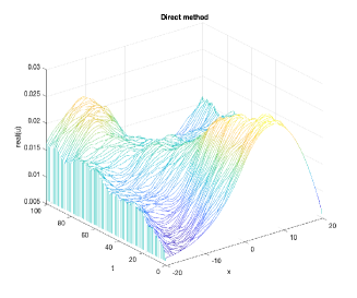
where $\mathcal{F}$ denotes the Fourier transform and $K$ is the diagonal matrix of Fourier coefficients $2\pi\mathrm{i}k$. In practice we use the fast Fourier transform and its inverse. We chose $\Delta t=0.001$ and the number of Fourier modes is $2^{8}$. The result is shown in the top two panels in Figure 1.

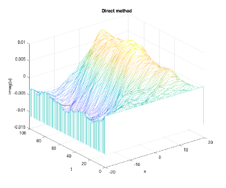
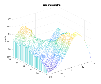
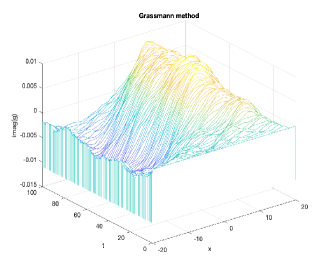
Second, in the Grassmann–Pöppe method, given the initial profile $p_{0}=p_{0}(x)$ we analytically advance the Fourier transform $\mathcal{F}(p_{0})$ of the initial data in Fourier space to any time of interest $t\in[0,T]$, where $T=100$. To generate $p=p(x,t)$ at that time, we then compute the inverse Fourier transform. In other words we compute the approximation $\hat{p}(x,t)=\mathcal{F}^{-1}(\exp(t(\mu_{2}K^{2}+\mu_{3}K^{3}+\mu_{4}K^{4}))\mathcal{F}(p_{0}))$ for any given time $t$. We then compute an approximation $\hat{q}=\hat{q}(y,z;x,t)$ at the time $t$ by approximating the integral in the prescription for $q$ above by a left-hand Riemann sum. To generate an approximation $\hat{g}$ for $g=g(y,z;x,t)$ at that time we approximate the integral in the linear Fredholm integral equation prescribing $g$ above by a left-hand Riemann sum and solve the resulting linear algebraic system of equations for $\hat{g}=\hat{g}(y,z;x,t)$. An approximation to the solution of the commutative fourth order quintic nonlinear Schrödinger equation is then $\hat{g}(0,0;x,t)$. The result is shown in the middle two panels in Figure 1. The magnitude of the difference between $\hat{g}(0,0;x,t)$ and $u_{m}$ is shown in the lower left panel. The lower right panel shows the magnitude of the Fredholm determinant $\det({\mathrm{id}}+\hat{Q}(x,t))$, where $\hat{Q}=\hat{Q}(x,t)$ is the linear operator associated with the kernel function $\hat{q}=\hat{q}(y,z;x,t)$.

Figure 1. We plot the solution to the commutative version of the fourth order quintic nonlinear Schödinger equation from Theorem 3.1. We chose the parameter values $\mu_{2}=-\mathrm{i}$, $\mu_{3}=1$ and $\mu_{4}=\mathrm{i}$. The top panels show the real and imaginary parts computed using a direct integration approach, while the middle panels show the corresponding real and imaginary parts computed using the Grassmann–Pöppe method. The bottom left panel shows the magnitude of the difference between the two computed solutions. The bottom right panel shows the evolution of the magnitude of the Fredholm determinant of $Q=Q(x,t)$.

Remark 4.1 (Periodic boundary conditions).

Our main result in Theorem 3.1 concerned the fourth order quintic nonlinear Schrödinger equation on the real line. The numerical simulations above are based on Fourier spectral approximations on the domain $[-L/2,L/2]$ with periodic boundary conditions. Indeed in the first step of the Grassmann–Pöppe method above we generate approximate solutions to the linear “base” partial differential equation by taking the inverse fast Fourier transform of the exact spectral representation for the solution. Our numerical simulations shown in Figure 1 demonstrate the Grassmann–Pöppe method appears to work perfectly well in the periodic context. However this does require further investigation, both analytically and numerical analytically.

Remark 4.2 (Korteweg de Vries and nonlinear Schrödinger).

This Grassmann–Pöppe method was used to generate approximate solutions to the standard Korteweg de Vries and nonlinear Schrödinger equations in Doikou et al. [19].

Remark 4.3 (Initial data).

In principle we could generate the numerical solutions using the Grassmann–Pöppe approach from given initial data $g_{0}=g_{0}(x)$ for the kernel function $g=g(0,0;x,0)$. The initial data $p_{0}$ for the linearised partial differential system for $p=p(x,t)$ can be computed from $g_{0}$ via ‘scattering’, as suggested for example by McKean [48].

Remark 4.4 (Grassmann–Pöppe single time evaluation).

We emphasise the following efficiency property of the Grassmann–Pöppe method. Given the initial data $p_{0}$, we compute its fast Fourier transform $\hat{p}_{0}=\hat{p}_{0}(k)$, for a finite set of wavenumbers $k$. We then advance the individual $k$-modes of $\hat{p}_{0}$ to any given time $t>0$ via the Fourier flow map $\exp\bigl{(}\Delta t(\mu_{2}(2\pi\mathrm{i}k)^{2}+\mu_{3}(2\pi\mathrm{i}k)^{3}+\mu_{4}(2\pi\mathrm{i}k)^{4})\bigr{)}$, corresponding to the linear partial differential equation prescribing $p=p(x,t)$. We can thus generate the Fourier coefficients $\hat{p}=\hat{p}(k,t)$ at any given time in one single step. We generate an approximation for $p=p(x,t)$ by then computing the inverse fast Fourier transform. And then finally we can generate $g=g(y,z;x,t)$ by solving the linear Fredholm equation at that time $t>0$, as described above. In contrast, the direct numerical simulation method requires computing the solution over successive small time steps to evaluate the solution at any time $t>0$.

5. Discussion

The advantages of the method we present to establish integrability for the generalised non-commutative fourth order quintic nonlinear Schrödinger equation, based on Pöppe’s Hankel operator approach are as follows. First, the method is abstract. Once the Fredholm equation $P=G({\mathrm{id}}+Q)$ is established the computation proceeds entirely at the operator level. The key initial ingredients are that the scattering data $P$ is a Hankel operator and depends on the parameters $x$ and $t$, and satisfies an evolution in $t$ linear equation involving a derivation operation with respect to $x$. And then the auxiliary data $Q$ is assigned appropriately in terms of $P$. Second, with this in hand, we can proceed in the operator algebra, to which a derivation operation can be applied, once we endow that algebra with a kernel product rule associated with the Hankel components. The procedure to establish a closed-form nonlinear kernel equation is then direct and elementary, only requiring basic calculus.

The observant reader will have noticed in the proof of Theorem 3.1 that, once we computed $\partial_{t}G-d(\partial)G$ in Step 1, the remaining Steps 2–9 in the proof were a collating exercise, once we applied the kernel bracket operator at the very beginning of Step 2. Indeed retrospectively we note the following. Step 2 dealt with the terms with factor $\mu_{2}$, i.e. those associated with the second order part of $d(\partial)$. The key identity in Step 2 helping to establish a closed nonlinear form is identity (i) in Lemma 2.6 for $\partial[PU\tilde{P}]$. Step 3 dealt with the terms with factor $\mu_{3}$, i.e. those associated with the third order part of $d(\partial)$. The key identity in Step 3 that established a closed nonlinear form is identity (ii) in Lemma 2.6 for $\partial[PU(\partial\tilde{P})]$, in addition to identity (i). Then in Steps 4–8, which dealt with the terms with factor $\mu_{4}$, the key identity was (iii) in Lemma 2.6 for $\partial[PU(\partial^{2}\tilde{P})]$, in addition to the previous two. Indeed the main work in establishing our main result in Theorem 3.1 was the proof of identities (i)–(iii) in Lemma 2.6. It is likely the proof of the Lemma can be simplified further. This suggests a key identity for the quintic order case, i.e. when the order of $d(\partial)$ is five, will involve an analogous expression for $\partial[PU(\partial^{3}\tilde{P})]$. This is the last case presented in Nijhoff et al. [52]. An explicit closed-form expression for all orders is obviously of interest. This could perhaps be achieved via a non-commutative generalisation of the recursion relation for the nonlinear Schrödinger hierarchy, see for example Pöppe [57] or Matveev and Smirnov [47], and/or via an algebraic combinatorial approach using algebraic structures analogous to those in Malham and Wiese [45], Ebrahimi–Fard et al. [21] or Ebrahimi-Fard et al. [22].

Some final observations are as follows. In Section 2 we discussed how a solution to the linear Fredholm equation for $G$ exists provided the determinant $\det({\mathrm{id}}+Q)\neq 0$. This is guaranteed locally in time under the conditions stated therein. Recall $Q$ is prescribed directly and solely in terms of $P$ and $P^{\dagger}$. Hence the evolution of $P$ and thus the determinant $\det({\mathrm{id}}+Q)$ determines the existence of $G$. If the determinant becomes zero at some time $t$ then the solution $G$ may become singular. More specifically, depending on the route to singularity, certain eigenvalues of $G$ will become singular; see Beck and Malham [10]. However, such singular behaviour in the context of Grassmannian flows simply indicates a poor choice of representative coordinate patch. By changing to another suitable patch, which is always possible, the solution can be continued. A careful analysis of this scenario is required. Additionally a careful numerical analysis of the Grassmann–Pöppe method we presented in Section 4 is also required.

References

- [1] A. Abbondandolo, P. Majer, Infinite dimensional Grassmannians, J. Operator Theory 61(1), 19–62 (2009).
- [2] M.J. Ablowitz, Z.H. Musslimani, Integrable nonlocal nonlinear Schrödinger equation, Phys. Rev. Lett. 110, 064105 (2013).
- [3] M.J. Ablowitz, Z.H. Musslimani, Integrable nonlocal nonlinear equations, Stud. Appl. Math. 139(1) (2017).
- [4] M.J. Ablowitz, Z.H. Musslimani, Integrable nonlocal asymptotic reductions of physically significant nonlinear equations, J. Phys. A: Math. Theor. 52, 15LT02 (2019).
- [5] M.J. Ablowitz, B. Prinari, D. Trubatch, Discrete and Continuous Nonlinear Schrödinger Systems, Cambridge University Press (2004).
- [6] M.J. Ablowitz, A. Ramani, H. Segur, A connection between nonlinear evolution equations and ordinary differential equations of P-type. II, Journal of Mathematical Physics 21, 1006–1015 (1980).
- [7] G.P. Agrawal, Applications of nonlinear fiber optics, Academic Press (2001).
- [8] E. Andruchow, G. Larotonda, Lagrangian Grassmannian in infinite dimension, Journal of Geometry and Physics 59, 306–320 (2009).
- [9] W. Bauhardt, Ch. Pöppe, The Zakharov–Shabat inverse spectral problem for operators, J. Math, Phys. 34(7), 3073–3086 (1993).
- [10] M. Beck, S.J.A. Malham, Computing the Maslov index for large systems, PAMS 143, 2159–2173 (2015).
- [11] M. Beck, A. Doikou, S.J.A. Malham, I. Stylianidis, Grassmannian flows and applications to nonlinear partial differential equations, Proc. Abel Symposium (2018).
- [12] M. Beck, A. Doikou, S.J.A. Malham, I. Stylianidis, Partial differential systems with nonlocal nonlinearities: generation and solutions, Phil. Trans. R. Soc. A 376(2117) (2018).
- [13] M. Ben–Artzi, H. Koch, J.C. Saut, Dispersion estimates for fourth order Schrödinger equations, C.R. Math. Acad. Sci. Sér. 1 330, 87–92 (2000).
- [14] G. Blower, S. Newsham, On tau functions associated with linear systems, Operator theory advances and applications: IWOTA Lisbon 2019. ed. Amelia Bastos; Luis Castro; Alexei Karlovich. Springer Birkhäuser, 2020. (International Workshop on Operator Theory and Applications).
- [15] T. Boulenger, E. Lenzmann, Blowup for biharmonic NLS, arXiv:1503.01741v2, (2015).
- [16] A. Degasperis, S. Lombardo, Multicomponent integrable wave equations: II. Soliton solutions, J. Phys. A: Math. Theor. 42(38) (2009).
- [17] S.T. Demiray, Y. Pandir, H. Bulut, All exact travelling wave solutions of Hirota equation and Hirota–Maccari system, Optik 127, 1848–1859 (2016).
- [18] A. Doikou, S.J.A. Malham, I. Stylianidis, Grassmannian flows and applications to non-commutative non-local and local integrable systems, Physica D 415, 132744 (2021).
- [19] A. Doikou, S.J.A. Malham, I. Stylianidis, A. Wiese, Applications of Grassmannian flows to nonlinear systems, submitted (2020).
- [20] F.J. Dyson, Fredholm determinants and inverse scattering problems, Commun. Math. Phys. 47, 171–183 (1976).
- [21] K. Ebrahimi–Fard, A. Lundervold, S.J.A. Malham, H. Munthe–Kaas, A. Wiese, Algebraic structure of stochastic expansions and efficient simulation, Proc. R. Soc. A 468, 2361–2382 (2012).
- [22] K. Ebrahimi–Fard, S.J.A. Malham, F. Patras, A. Wiese, The exponential Lie series for continuous semimartingales, Proc. R. Soc. A 471 (2015).
- [23] N. Ercolani, H.P. McKean, Geometry of KDV (4): Abel sums, Jacobi variety, and theta function in the scattering case, Invent. Math. 99, 483–-544 (1990).
- [24] G. Fibich, B. Ilan, G. Papanicolaou, Self-focusing with fourth order dispersion, SIAM J. Appl. Math. 62(4), 1437–1462 (2002).
- [25] A.S. Fokas, Integrable multidimensional versions of the nonlocal nonlinear Schrödinger equation, Nonlinearity 29, 319–324 (2016).
- [26] A.S. Fokas, M.J. Ablowitz, Linearization of the Kortweg de Vries and Painlevé II Equations, Phys. Rev. Lett. 47, 1096 (1981).
- [27] A. S. Fokas, B. Pelloni, Unified Transform for Boundary Value Problems: Applications and Advances, Society for Industrial and Applied Mathematics (2014).
- [28] A.P. Fordy, P.P. Kulish, Nonlinear Schrödinger Equations and Simple Lie Algebras, Commun. Math. Phys. 89, 427–443 (1983).
- [29] V.S. Gerdjikov, A. Saxena, Complete integrability of nonlocal nonlinear Schrödinger equation, J. Math. Phys. 58, 013502 (2017).
- [30] G.G. Grahovski, A.J. Mohammed, H. Susanto, Nonlocal Reductions of the Ablowitz-Ladik Equation, Theor. Math. Phys. 197, 1412–1429 (2018).
- [31] S. Grellier, P. Gerard, The cubic Szegö equation and Hankel operators, Astérisque 389 (2017), Société Mathématique de France, Paris.
- [32] S. Grudsky, A. Rybkin, On classical solutions of the KdV equation, Proc. London Math. Soc. 121, 354–371 (2020).
- [33] S. Grudsky, A. Rybkin, Soliton theory and Hankel operators, SIAM J. Math. Anal. 47(3), 2283–2323 (2015).
- [34] Y.-Y. Guan, B. Tian, H.-L. Zhen, Y.-F. Wang, J. Chai, Soliton solutions of a generalised nonlinear Schrödinger–Maxwell–Bloch system in the erbium-doped optical fibre, Zeitschrift für Naturforschung 71(3), doi.org/10.1515/zna-2015-0466 (2016).
- [35] R. Guo, H.-Q. Hao, X.-S. Gu, Modulation instability, breathers, and bound solitons in an erbium-doped fiber system with higher-order effects, Abstract and Applied Analysis 2014, dx.doi.org/10.1155/2014/185654 (2014).
- [36] M. Gürses, A. Pekcan, Superposition of the coupled NLS and MKdV Systems, Appl. Math. Lett. 98, 157–163 (2019).
- [37] M. Gürses, A. Pekcan, Nonlocal modified KdV equations and their soliton solutions, Commun. Nonlinear Sci. Numer. Simul. 67, 427–448 (2019).
- [38] M. Gürses, A. Pekcan, Nonlocal nonlinear Schrodinger equations and their soliton solutions, J. Math. Phys. 59, 051501 (2018).
- [39] M. Gürses, A. Pekcan, Nonlocal KdV equations, arXiv:2004.07144 (2020).
- [40] Z.-Z. Kang, T.-C. Xia, W.-X. Ma, Riemann–Hilbert approach and -soliton solution for an eighth-order nonlinear Schrödinger equation in an optical fiber, Advances in Difference Equations 188, doi.org/10.1186/s13662-019-2121-5 (2019).
- [41] V.I. Karpman, Stabilization of soliton instabilities by higher order dispersion: Fourth-order nonlinear Schrödinger-type equations, Phys. Rev. E 53, 1336-1339 (1996).
- [42] V.I. Karpman, A.G. Shagalov, Stability of solitons described by nonlinear Schrödinger-type equations with higher-order dispersion, Phys. D 144, 194–210 (2000).
- [43] C. Kwak, Periodic fourth order cubic NLS: Local well-posedness and non-squeezing property, arXiv:1708.00127v2, (2018).
- [44] S.Y. Lou, F. Huang, Alice–Bob Physics: Coherent solutions of nonlocal KdV systems, Scientific Reports 7: 869 (2017).
- [45] S.J.A. Malham, A. Wiese, Stochastic expansions and Hopf algebras, Proc. R. Soc. A 465, 3729–3749 (2009).
- [46] S.V. Manakov, On the theory of two-dimensional stationary self-focusing of electromagnetic waves, Sov. Phys. - JETP 38(2), 248–253 (1974).
- [47] V.B. Matveev, A.O. Smirnov, AKNS and NLS hierarchies, MRW solutions, breathers, and beyond, Journal of Mathematical Physics 59, 091419 (2018).
- [48] H.P. McKean, Fredholm determinants, Cent. Eur. J. Math. 9, 205–243 (2011).
- [49] D. Mihalache, N.-C. Panoiu, F. Moldoveanu, D.-M. Baboiu, The Riemann–Hilbert problem method for solving a perturbed nonlinear Schrödinger equation describing pulse propagation in optic fibres, J. Phys. A: Math. Gen. 27, 6177–6189 (1994).
- [50] D. Mumford Tata lectures on Theta II, Modern Birkhauser Classics (1984).
- [51] K. Nakkeeran, Optical solitons in erbium doped fibers with higher order effects, Physics Letters A 275, 415–418 (2000).
- [52] F.W. Nijhoff, G.R.W. Quispel, J. Van Der Linden, H.W. Capel, On some linear integral equations generating solutions of nonlinear partial differential equations, Physica A 119, 101–142 (1983).
- [53] T. Oh, Y. Wang, Global well-posedness of the periodic cubic fourth order NLS in negative Sobolev spaces, arXiv:1707.02013v2, (2018).
- [54] B. Pausader, The cubic fourth order Schrödinger equation, Journal of Functional Analysis 256, 2473–2517 (2009).
- [55] D.E. Pelinovsky, Y.A. Stepanyants, Helical solitons in vector modified Korteweg-de Vries equations, Physics Letters A 382, 3165–3171 (2018).
- [56] C. Pöppe, Construction of solutions of the sine-Gordon equation by means of Fredholm determinants, Physica D 9, 103–139 (1983).
- [57] C. Pöppe, The Fredholm determinant method for the KdV equations, Physica D 13, 137–160 (1984).
- [58] C. Pöppe, General determinants and the function for the Kadomtsev-Petviashvili hierarchy, Inverse Problems 5, 613–630 (1984).
- [59] C. Pöppe, D.H. Sattinger, Fredholm determinants and the function for the Kadomtsev-Petviashvili hierarchy, Publ. RIMS, Kyoto Univ. 24, 505–538 (1988).
- [60] I. Posukhovskyi, A. Stefanov, On the normalized ground states for the Kawahara equation and a fourth order NLS, arXiv:1711.00367v3, (2020).
- [61] A. Pressley, G. Segal, Loop groups, Oxford Mathematical Monographs, Clarendon Press, Oxford (1986).
- [62] Y. Ren, Z.-Y. Yang, C. Liu, W.-H. Xu, W.-L. Yang, Characteristics of optical multi-peak solitons induced by higher-order effects in an erbium-doped fiber system, Eur. Phys. J. D 70, DOI: 10.1140/epjd/e2016-70079-7 (2016).
- [63] M. Sato, Soliton equations as dynamical systems on a infinite dimensional Grassmann manifolds. RIMS 439, 30–46 (1981).
- [64] M. Sato, The KP hierarchy and infinite dimensional Grassmann manifolds, Proceedings of Symposia in Pure Mathematics 49 Part 1, 51–66 (1989).
- [65] G. Segal, G. Wilson, Loop groups and equations of KdV type, Inst. Hautes Etudes Sci. Publ. Math. 61, 5-–65 (1985).
- [66] Simon B 2005 Trace ideals and their applications, 2nd edn. Mathematical Surveys and Monographs, vol. 120. Providence, RI: AMS.
- [67] I. Stylianidis, Grassmannian flows: applications to PDEs with local and nonlocal nonlinearities, PhD Thesis, under review (2021).
- [68] L. Wang, S. Li, F.-H. Qi, Breather-to-soliton and rogue wave-to-soliton transitions in a resonant erbium-doped fiber system with higher-order effects, Nonlinear Dyn. 85, 389–398 (2016).
- [69] L. Wang, X. Wu, H.-Y. Zhang, Superregular breathers and state transitions in a resonant erbium-doped fiber system with higher-order effects, Physics Letters A 382, 2650–2654 (2018).
- [70] L.H. Wang, K. Porsezian, J.S. He, Breather and rogue wave solutions of a generalized nonlinear Schrödinger equation, Physical Review E 87, 053202 (2013).
- [71] Q.-M. Wang, Y.-T. Gao, C.-Q. Su, D.-W. Zuo, Solitons, breathers and rogue waves for a higher order nonlinear Schrödinger–Maxwell–Bloch system in an erbium-doped fiber system, Phys. Scr. 90, 105202 (2015).
- [72] V.E. Zakharov, A.B. Shabat, A scheme for integrating the nonlinear equations of mathematical physics by the method of the inverse scattering problem I, Funct. Anal. Appl. 8, 226–235 (1974).
- [73] V.E. Zakharov, A.B. Shabat, Integration of nonlinear equations of mathematical physics by the method of inverse scattering II, Funct. Anal. Appl. 13(3), 166–-174 (1979).