High-resolution spectroscopy of SN 2017hcc and its blueshifted line profiles from post-shock dust formation

Abstract

SN 2017hcc was remarkable for being a nearby and strongly polarized superluminous Type IIn supernova (SN). We obtained high-resolution echelle spectra that we combine with other spectra to investigate its line profile evolution. All epochs reveal narrow P Cygni components from pre-shock circumstellar material (CSM), indicating an axisymmetric outflow from the progenitor of 40-50 km s^-1. Intermediate-width and broad components exhibit the classic evolution seen in luminous SNe IIn: symmetric Lorentzian profiles from pre-shock CSM lines broadened by electron scattering at early times, transitioning at late times to multi-component, irregular profiles coming from the SN ejecta and post-shock shell. As in many SNe IIn, profiles show a progressively increasing blueshift, with a clear flux deficit in red wings of the intermediate and broad velocity components after day 200. This blueshift develops after the continuum luminosity fades, and in the intermediate-width component, persists at late times even after the SN ejecta fade. In SN 2017hcc, the blueshift cannot be explained as occultation by the SN photosphere, pre-shock acceleration of CSM, or a lopsided explosion or CSM. Instead, the blueshift arises from dust formation in the post-shock shell and in the SN ejecta. The effect has a wavelength dependence characteristic of dust, exhibiting an extinction law consistent with large grains. Thus, SN 2017hcc experienced post-shock dust formation and had a mildly bipolar CSM shell, similar to SN 2010jl. Like other superluminous SNe IIn, the progenitor lost around 10 $M_{\odot}$ due to extreme eruptive mass loss in the decade before exploding.

1 INTRODUCTION

1.1 Eruptive pre-SN mass loss

Throughout their lives, massive stars shed mass through steady winds, but these winds can be punctuated by episodic mass loss events (Smith, 2014). Observationally-derived wind mass-loss rates have been revised downward compared to rates still used in most stellar evolution codes, undermining some basic predictions of single-star models (Smith, 2014). Mass-loss rates have been reduced for both line-driven winds of hot stars (Bouret et al., 2005; Fullerton et al., 2006; Puls et al., 2008; Sundqvist et al., 2019), and more recently also for dusty red supergiant (RSG) winds (Beasor et al., 2020).

On the other hand, there has been a shift to stronger influence of eruptive mass loss (Smith & Owocki, 2006) and binary mass exchange and stripping (Sana et al., 2012; Moe & Di Stefano, 2017; Götberg et al., 2018). Eruptive mass loss like luminous blue variables (LBVs) or violent binary interaction are less sensitive to metallicty than line-driven winds (Smith & Owocki, 2006; Götberg et al., 2017), making them more relevant to supernovae (SNe) that arise in lower-metallicity regions. Eruptive LBV-like mass loss and violent binary interaction may be related, since mergers and mass gainers are needed to explain various properties of LBVs (Justham et al., 2014; Smith & Tombleson, 2015; Aghakhanloo et al., 2017; Smith et al., 2018a).

Eruptive mass loss has become especially prominent in the case of strongly interacting SNe of Types IIn (SNe IIn) and Ibn (SNe Ibn), where observed signatures of interaction with dense circumstellar material (CSM) indicate extreme and short-lived mass-loss phases immediately preceding core collapse; see Smith (2017) and Smith (2014) for reviews. The specific mechanism(s) of the eruptive pre-SN mass loss remains uncertain, but it requires a trigger synchronized with core-collapse. Some proposed mechanisms include energy deposited in the envelope by wave driving in advanced nuclear burning phases (Quataert & Shiode, 2012; Shiode & Quataert, 2014; Fuller, 2017; Fuller & Ro, 2018), the pulsational pair instability or other late-phase burning instabilities (Woosley et al., 2007; Woosley, 2017; Smith & Arnett, 2014; Renzo et al., 2020), or an inflation of the progenitor’s radius (perhaps caused by the previous mechanisms) that triggers violent binary interaction like collisions or mergers before core collapse (Smith & Arnett, 2014). Of these, only the last predicts highly asymmetric distributions of CSM (disk-like or bipolar), relevant to asymmetric line profile shapes and high polarization seen in SNe IIn.

An extreme case of eruptive pre-SN mass loss is found in super-luminous SNe (SLSNe) with exceptionally strong CSM interaction, where the very high luminosity is thought to result from an explosion with normal to high explosion energy (1-5$\times$10⁵¹ erg) running to a very high mass of CSM, usually of order a few to 20 M_⊙. Some well studied examples include SN 2006gy, SN 2006tf, SN 2008am, SN 2003ma, SN 2015da, and SN 2010jl (Smith et al., 2007, 2010a; Smith & McCray, 2007; Chatzopoulous et al., 2011; Rest et al., 2011; Tartaglia et al., 2020; Gall et al., 2014; Fransson et al., 2014; Jencson et al., 2016; Woosley et al., 2007) These events have high efficiency in converting ejecta kinetic energy into luminosity of order $10\%-50\%$ or more (van Marle et al., 2010), with total radiated energy budgets $\ga$10⁵¹ erg.

1.2 Dust formation in interacting SNe

An important feature of strongly interacting SNe is the formation of a cold dense shell (CDS) between the forward and reverse shocks (Chugai, 2001; Chugai et al., 2004; Smith et al., 2008b). Efficient radiative cooling causes the dense post-shock gas to collapse into a thin, dense, clumpy, and probably well-mixed layer (van Marle et al., 2010). This rapid cooling that forms a dense shell is a unique feature of interacting SNe, causing their defining narrow-line spectra and their high luminosity. This rapid cooling and high density may also trigger early dust formation.

There are 3 common observational signatures of new dust formation in SNe: (1) a strengthening IR excess consistent with dust emission, (2) an increased rate of fading in the optical continuum that may be attributed to increased extinction from new dust, and (3) a progressive and systematic blueshift in emission-line profiles caused by dust that preferentially obscures the redshifted portions of the explosion. Each of these alone is somewhat ambiguous — an IR excess could be due to an IR echo from CSM dust (Fox et al., 2011; Andrews et al., 2011), the rate of fading can depend on other factors unrelated to dust, and blueshifted line profiles can arise from asymmetry in the ejecta or CSM, or optical depth effects at early times — but seeing all three together, as in the case of SN 1987A (Danziger et al., 1989; Lucy et al., 1989; Gehrz & Ney, 1989; Wooden et al., 1993; Colgan et al., 1994), gives a strong indication that new dust has formed. Of these three, the third is unique in helping to diagnose the location of the dust because of the different charactistic expansion speeds in the unshocked CSM, SN ejecta, and the post-shock CDS. The characteristic blueshift of emission lines is fairly common in interacting SNe, and has been tied to dust formation in the SN ejecta and post-shock CDS.

The first clear case of an interacting SN that showed all three signatures of dust formation was SN 2006jc, where the line-profile evolution of He i lines (this was a Type Ibn) indicated that new dust formed in the post-shock CDS (Smith et al., 2008a). This blueshift coincided in time with an IR excess and fading in the continuum, but also a burst of X-ray emission and He ii $\lambda$4686 emission (Immler et al., 2008; Smith et al., 2008a; Di Carlo et al., 2008), indicating that the SN shock crashing into a dense shell is what triggered the rapid onset of dust formation only 50-100 days after discovery. The rapid post-shock dust formation may be analogous to what happens in dust-forming colliding-wind binaries like the WC+OB system WR 140 (Hackwell, Gehrz, & Grasdalen, 1979; Williams et al., 1990; Monnier et al., 2002) and $\eta$ Car (Smith, 2010). Similar blueshifted profiles have been seen in a number of H-rich interacting SNe, including SN 2006tf (Smith et al., 2008b), SN 2005ip (Smith et al., 2009a; Fox et al., 2009; Smith et al., 2017), SN 2007rt (Trundle et al., 2009), SN 2007od (Andrews et al., 2010), SN 2010bt (Elias-Rosa et al., 2018), and SN 2010jl (discussed below).

The line profile blueshift seen in interacting SNe has usually been interpreted as post-shock or ejecta dust formation. Line profile blueshift gives a more direct probe of the dust location, as noted above, but it is harder to infer the dust mass from extinction’s effect on line profiles without detailed models and assumptions (Bevan et al., 2018, 2020). One should realize that these options for the location of the dust are not mutually exclusive. Dust may form in both the CDS and the inner SN ejecta at various times, and there may also be pre-existing CSM dust. In fact, we expect pre-existing dust in the CSM for SNe IIn because of extreme eruptive mass loss (like LBVs or extreme RSGs), and those are the same progenitors most likely to have the high CSM density to trigger efficient radiative cooling and collapse of the CDS, which in turn permits efficient dust formation in the post-shock region. There has, however, been discussion in the literature about alternatives to dust formation to explain the blueshifts, as illustrated by the case of SN 2010jl.

1.3 SN 2010jl

SN 2010jl was among the nearest SLSNe IIn, leading to considerable observational attention with high-quality optical/IR photometry and spectroscopy (Andrews et al., 2011; Stoll et al., 2011; Smith et al., 2011a, 2012a; Zhang et al., 2012; Fox et al., 2013; Maeda et al., 2013; Gall et al., 2014; Fransson et al., 2014; Borish et al., 2015; Williams & Fox, 2015; Jencson et al., 2016; Sarangi et al., 2018; Chugai, 2018; Bevan et al., 2020). While pre-existing CSM dust probably contributed to the observed IR excess (Andrews et al., 2011), even early spectra revealed a prominent blueshift in line profiles that strengthened with time (Smith et al., 2012a; Gall et al., 2014).

The systematic blueshift of line profiles and their wavelength dependence (more pronouned at shorter wavelengths) led to the suggestion that, like SN 2006jc, SN 2010jl experienced new dust formation in the post-shock region of the CDS (Smith et al., 2012a). Several additional studies confirmed these signs of dust formation in the post-shock CDS and investigated the dust properties, including additional late-time spectra, IR data, and models (Gall et al., 2014; Sarangi et al., 2018; Chugai, 2018; Bevan et al., 2020). Dust may have been pre-existing in the CSM, and dust may have formed in the ejecta (Andrews et al., 2011; Bevan et al., 2020).

The conclusion that the blueshift in line profiles was influenced by dust formation in the CDS was not, however, adopted by all authors. Namely, Fransson et al. (2014) proposed a different picture where the blueshifted profiles were caused by acceleration of asymmetric pre-shock CSM along the line of sight, and where the broad components were caused by electron scattering of the narrow CSM emission from that accelerated CSM. This explanation did not account for why the narrow components from the unshocked CSM were not blueshifted even though the broader components had a blueshifted centroid, or why there was a wavelength dependence to the asymmetry. Subsequent radiative transfer models of SN 2010jl’s spectrum (Dessart et al., 2015) found that accelerated pre-shock CSM could not explain the observed blueshift in line profile shape, or their behavior with time. Dessart et al. (2015) showed that while the early symmetric line profiles were caused by electron scattering of narrow CSM emission, the broad blueshifted profiles at later times arises in the post-shock CDS. These models revealed a blueshifted emission bump that could arise even without dust, at least initially, because the photosphere in the CSM interaction region could block the redshifted side of the CDS, as noted earlier by Smith et al. (2012a). Again, however, this mechanism would not account for the observed wavelength dependence of the blueshift (Smith et al., 2012a; Gall et al., 2014).

If the systematic blueshift of the broader components were due mostly to an optical depth effect in the CDS, as seen in these models for SN 2010jl spectra up until about day 200 (Dessart et al., 2015), then there is a clear prediction for the late-time evolution. Namely, at late times these lines should become more symmetric, as the optical depth drops and the continuum luminosity fades, revealing emission from the receding side (Smith et al., 2012a; Dessart et al., 2015). This did not happen in SN 2010jl. The continuum luminosity dropped around day 300, but the blueshift persisted even in spectra beyond day 1000 (Fransson et al., 2014). This would seem to clearly rule out high continuum optical depths and electron scattering of accelerated CSM as the explanation for the persistent blueshift, instead favoring dust formation in the post-shock shell of SN 2010jl (Smith et al., 2012a; Gall et al., 2014; Sarangi et al., 2018; Bevan et al., 2020).

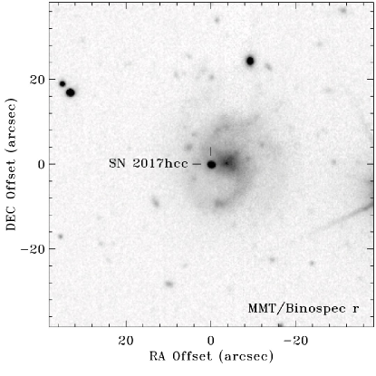
Figure 1: A late-time $r$-band image of SN 2017hcc and its host galaxy taken on 2019 July 9 using Binospec on the MMT. SN 2017hcc is found about 0.5 arcsec south and 4.5 arcsec east of the center of its spiral host galaxy.

1.4 SN 2017hcc

SN 2017hcc was discovered on 2017 October 2 by the Asteroid Terrestrial-impact Last Alert System (ATLAS; Tonry 2011), and was classified as a young Type IIn event (Prieto et al., 2017). It was reportedly located a few arcsec southeast of the center of an anonymous host galaxy. Figure 1 shows an MMT/Binospec image of the SN (see details below), indicating that it is located 0.5 arcsec south and 4.5 arcsec east of the center of its host galaxy, and appears coincident with the leading edge of a spiral arm. The SN was discovered within a few days of explosion, judging by a non-detection a few days earlier. Following Prieto et al. (2017), who presented early photometry, we adopt an explosion date of 2017 Oct 1.4, which we set as $t$ = 0 in this study. As in Prieto et al. (2017), we adopt a redshift of $z$=0.0168 and a distance of 73 Mpc. We also adopt $E(B-V)$=0.0285 mag for our line-of-sight through the Milky Way interstellar medium (Schlafly & Finkbeiner, 2011) to deredden our spectra, although this has little impact on our analysis of line profiles. At this distance, its peak $V$ magnitude of 13.7 mag implies an absolute magnitude of $-$20.7 mag (Prieto et al., 2017), making SN 2017hcc a superluminous SN IIn. SN 2017hcc reached the peak of its $V$-band luminosity about 40-45 days after explosion (Prieto et al., 2017). This is a relatively slow rise, although not as slow as the unusual case of SN 2006gy, which took $\sim$70 days (Smith et al., 2007). SN 2017hcc was not detected at early times in either X-rays with Chandra or in the radio (Chandra et al., 2017; Nayana & Chandra, 2017), although such indicators are often faint at early times when X-ray and radio emission are absorbed.

Perhaps the most notable property of SN 2017hcc so far is that spectropolarimetry obtained soon after discovery by Mauerhan et al. (2017a) indicated very high continuum polarization of 4.8% or more. This may be the highest level of polarization seen in any SN to date, and points to significant asymmetry in the interaction region of this SN IIn. This asymmetry indicated by polarization is relevant to the interpretation of the observed evolution of emission-line profile shapes for SN 2017hcc that we discuss below. In section 2 we present our new spectroscopic observations, in section 3 we present results from the analysis of line profiles in our spectra, and in section 4 we discuss the interpretation of these line profiles and corresponding implications for the nature of the CSM and for dust formation in SN 2017hcc.

Table 1: Low resolution spectroscopy of SN 2017hcc

UT Date	daya	Tel./Instr.	grating	$\Delta\lambda$ ($\mu$m)
2017 10 26	25	MMT/Blue	1200	0.57-0.70
2017 10 27	26	Bok/BC	300	0.44-0.87
2017 11 19	49	MMT/Blue	1200	0.57-0.70
2017 12 09	69	Bok/BC	300	0.44-0.87
2017 12 15	75	MMT/Blue	1200	0.57-0.70
2017 12 28	88	MMT/Red	1200	0.62-0.70
2018 01 01	92	Bok/BC	300	0.44-0.87
2018 06 30	271	MMT/Blue	1200	0.57-0.70
2018 08 31	336	MMT/MMIRS	zJ/HK	1.0-2.3
2018 09 05	340	MMT/Blue	300	0.57-0.70
2018 10 18	382	MMT/Bino	600	0.51-0.75
2018 11 17	412	MMT/MMIRS	zJ/HK	1.0-2.3
2019 07 08	645	MMT/Bino	600	0.51-0.75
2019 11 02	762	MMT/Bino	600	0.51-0.75
2020 01 27	848	Mag/IMACS	1200	0.63-0.67

^aWe adopt 2017 Oct 1 as day zero, close to the explosion date inferred by Prieto et al. (2017).

2 OBSERVATIONS

2.1 Optical image

We obtained a deep $r$-band image of SN 2017hcc on 2019 July 9 (day 646) using the imaging mode of Binospec (Fabricant et al., 2019) on the Multiple Mirror Telescope (MMT). The image was reduced using a custom python pipeline and is shown in Figure 1. SN 2017hcc is located about 0.5 arcsec south and 4.5 arcsec east of the center of its spiral host galaxy (a foreground star or cluster projected near the galaxy nucleus would shift the centroid of the galaxy light slightly to the east in lower-resolution images). SN 2017hcc is therefore projected a total of 4.53 arcsec from center, or $\sim$1.6 kpc from the nucleus at the adopted distance of 73 Mpc. Although the host galaxy is anonymous and does not appear in the NASA Extragalactic Database, according to SIMBAD, it is coincident with the UV source GALEX 2674128878581058535. The coordinates listed for this GALEX source are offset a few arcsec from the apparent center of the galaxy. SN 2017hcc appears to be located on the leading edge of an inner spiral arm or bar, although the ground-based angular resolution is insufficient to determine its proximity to any dust lanes or star forming regions.

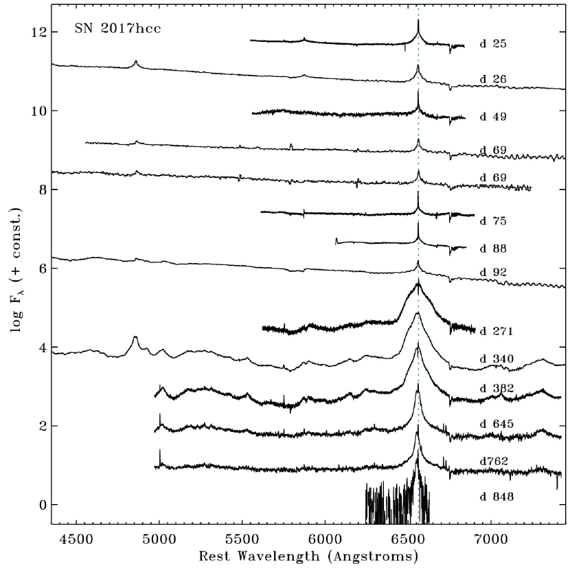
Figure 2: Sequence of low-resolution optical spectra from the MMT, Bok, and Magellan (see Table 1). Flux is on a log scale.

2.2 Low-resolution optical spectra

We obtained spectra of SN 2017hcc using the 6.5-m Multiple Mirror Telescope (MMT) with three different instruments, including the Bluechannel (BC) spectrograph, the Redchannel (RC) spectrograph, and the newly commissioned BinoSpec spectrograph (Fabricant et al., 2019). Each MMT Bluechannel or Redchannel observation was taken with a 1.0 arcsec slit and either the 1200 lines mm^-1 grating covering a range of approximately 5800–7000 Å, or the 300 lines mm^-1 grating covering a range of about 3600-8000 Å. Standard reductions were carried out using IRAF including bias subtraction, flat-fielding, and optimal extraction of the spectra. Flux calibration was achieved using spectrophotometric standards observed at an airmass similar to that of each science frame, and the resulting spectra were median combined into a single 1D spectrum for each epoch.

We obtained several late epochs of visual-wavelength spectra using Binospec on the MMT. These data were all taken using the 600 lines mm^-1 grating centered on 6300 Å  (covering a range of roughly 5100–7500 Å) and with a 1.0 arcsec slit. All data were reduced using the Binospec pipeline (Kansky et al., 2019), which includes an internal flux calibration into relative flux units from throughput measurements of spectrophotometric standard stars.

We obtained a few epochs of low-resolution optical spectra with the Boller & Chivens (B&C) spectrograph on the 2.3 m Bok telescope. We also obtained one late-time spectrum using the Inamori-Magellan Areal Camera and Spectrograph (IMACS; Dressler et al. 2011) mounted on the 6.5 m Baade telescope of the Magellan Observatory. Data reduction for these followed standard reduction for point sources in long-slit optical spectra, as above. Our low/moderate-resolution spectroscopic observations are summarized in Table 1, and all are plotted in Figure 2.

2.3 MIKE echelle spectra

We observed SN 2017hcc on three separate occasions using the Magellan Inamori Kyocera Echelle (MIKE), which is a double echelle spectrograph designed for use at the Magellan Telescopes at Las Campanas Observatory in Chile (Bernstein et al., 2003). We obtained observations of SN 2017hcc during its main luminosity peak on 2017 Oct 25 UT (a total exposure time of 2700 sec), and at two later epochs after it faded by several magnitudes on 2018 Jul 11 and Sep 17 UT (total exposure times of 5400 sec and 3600 sec, respectively). All three observations had good transparency and seeing (roughly 0.8 arcsec or better), and all had the 1 arcsec $\times$ 5 arcsec slit aperture aligned at the parallactic angle. This yields a resolving power $R$=$\lambda$/$\Delta\lambda$ of roughly 30,000, or a resolution of typically 10 km s^-1 (although we note that the achieved resolution measured from sky lines was somewhat narrower than this, about 8 km s^-1, because the seeing was better than the slit width on all three epochs).

The spectra were reduced using the latest version of the MIKE pipeline (written by D. Kelson). The reduced spectra were corrected for SN 2017hcc’s redshift of $z$ = 0.01686, and each epoch had velocities converted to the heliocentric reference frame (this correction matters for the narrow components from the pre-shock CSM). Figure 3 shows the region of the spectrum including the Na i D doublet useful for evaluating interstellar extinction and reddening, and also includes He i $\lambda$5876 emission from the SN. Figures 4 and 5 show the full line profiles of H$\alpha$ and H$\beta$, respectively. For H$\alpha$, the line center was located near the edge of two adjacent echelle orders, so to display the full profile in Figure 4, we spliced together two adjacent echelle orders. Because of the drop in sensitivity and the large throughput corrections needed at the ends of echelle orders, we checked the resulting overall shape of the line profile by comparing it to lower-resolution single-order spectra taken very close in time (see above). These are plotted in orange in Figure 4, showing very good agreement in overall line shape. Only a single echelle order is plotted for H$\beta$, because it was centered in the middle of an ehelle order. For H$\beta$, we caution that the red wing of the line is partly blended with Fe ii lines, so this should not be interpreted as excess redshifted H$\beta$ flux. For both H$\alpha$ and H$\beta$, the first epoch line profile is compared to a Lorentzian line profile shape (thick light-blue curve), meant to match the line wings with FWHM = 2000 km s^-1 for H$\alpha$ and 1600 km s^-1 for H$\beta$. Figure 6 shows examples of Gaussian components that may be fit to the day 351 H$\alpha$ line profile shape, discussed in more detail later.

Figure 7 zooms-in on the narrow components of H$\alpha$, H$\beta$, and H$\gamma$ seen in MIKE spectra, showing the P Cygni profiles arising from the unshocked CSM. For the first epoch, the “continuum” level is set at the continuum after subtraction of the Lorentzian profiles shown in Figures 4 and 5. For the two later epochs, the “continuum” for normalization refers to the flux level of the broader emission component within $\pm$400 km s^-1. Similarly, Figures 8 and 9 zoom-in on the narrow CSM components of He i $\lambda$5876 and $\lambda$6680, respectively, with both being compared to the narrow components of H$\beta$. (We do not show He i $\lambda$7065 because SN 2017hcc’s redshift caused this line to overlap with many narrow telluric absorption lines, complicating the interpretation of narrow P Cygni absorption features.)

Finally, Figure 10 compares the full line profile shapes of H$\alpha$ (black) and H$\beta$ (blue) superposed on one another. We have chosen to align these by scaling the line flux to match the shape of the blue wing of the emission line, in order to determine if there are any differences in the shape of the red wing. The H$\beta$ line strengths have therefore been scaled arbitrarily in flux above the continuum level. For the first early epoch, the profile shapes of H$\alpha$ and H$\beta$ agree remarkably well. For the later two epochs, however, the red wings of H$\beta$ are slightly depressed compared to H$\alpha$. This indicates that there is a wavelength dependence to the line shape that we discuss later.

2.4 Near-IR spectra

We obtained two epochs of near-IR spectra covering the $J$, $H$, and $K$, bands (roughly 1$-$2.3 $\mu$m) using the MMT and Magellan Infrared Spectrograph (MMIRS; McLeod et al., 2012) mounted on the MMT, with observations listed in Table 1. The standard long-slit zJ and HK single-order spectra were reduced using the MMIRS data reduction pipeline (Chilingarian et al., 2013). In this paper, we are most interested in the Pa$\beta$ 1.28 $\mu$m line profile shape, plotted along with H$\alpha$ line profiles in Figure 11.

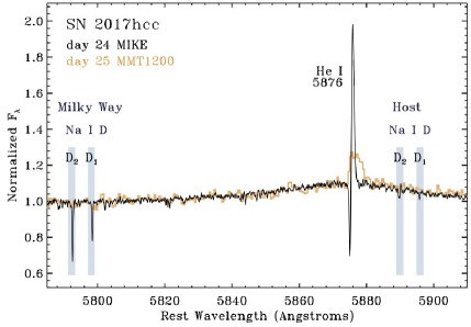
Figure 3: MIKE spectrum on day 24 in the region around Na i D and He i $\lambda$5876, shown in black. The moderate-resolution MMT/Bluechannel spectrum taken one day later with the 1200 lines mm^-1 grating is shown in orange for comparison. Expected locations of the D₁ and D₂ lines of the doublet are indicated by vertical blue bars for the redshift-corrected host galaxy and Milky Way components. Narrow P Cygni absorption of He i $\lambda$5876 is strong in the echelle spectrum, but is washed out in the moderate resolution spectrum, and even the strong Milky Way Na i D absorption is barely detected in the MMT spectrum.

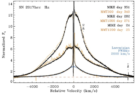
Figure 4: Full line profiles of H$\alpha$ as seen in the three epochs of MIKE spectra (black). The orange line profiles are from low- or moderate-resolution spectra taken around the same time, for comparison. Because the H$\alpha$ line wings are so broad and the line center was located near the end of an echelle order, we used one order for blueshifted velocities and the adjacent order for the red wing of the line. The blue solid curve shows a symmetric Lorentzian profile for comparison with the early epoch line profile shape. The flux is on a linear scale.

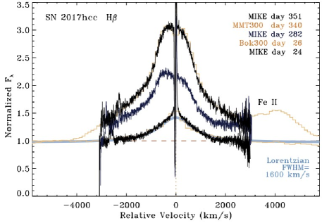
Figure 5: Same as Figure 4, but for H$\beta$. Zero velocity of H$\beta$ was located near the center of a MIKE echelle order, so we only show one full echelle order (there were slight flux mismatches and increased noise at the edges of adjacent orders. Aside from the edges of the orders, the line shapes in echelle spectra and lower resolution spectra are consistent. The bump at high positive velocity is emission from another line or lines (most likely Fe ii), rather than a strong excess of high velocity H$\beta$ emission. The flux is on a linear scale.

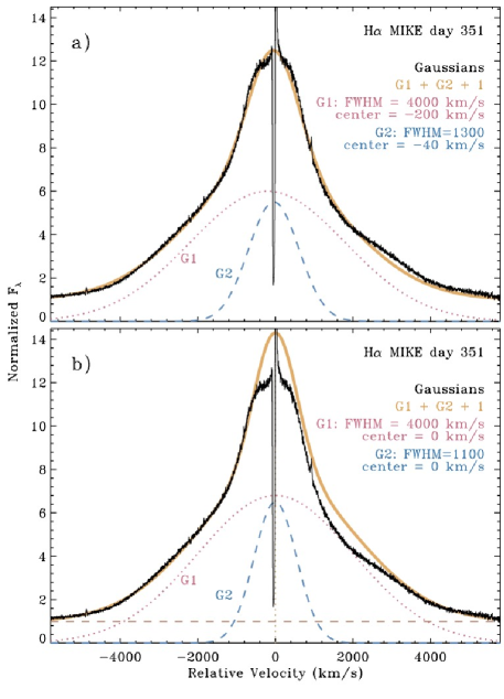
Figure 6: Full line profile of H$\alpha$ as seen in the day 352 MIKE spectrum, compared to to different multicomponent Gaussians. The top panel (a) shows two Gaussian profiles and their sum (plus continuum) where the centroids are allowed to be offset from zero, and the bottom (b) shows two similar Gaussians and their sum (plus continuum), but with the center fixed at 0 km s^-1, and where the sum is allowed to extend above the flux at low velocities and the red wing of the line (the excess flux may represent line flux lost from the intrinsic profile due to absorption).

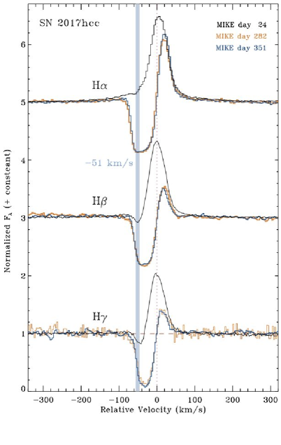
Figure 7: Detail showing the narrow components of the brightest Balmer lines H$\alpha$, H$\beta$, and H$\gamma$ in the three epochs of echelle spectra. For the first epoch of each, the observed profile was divided by an underlying broad Lorentzian (blue in Figure 4). For the two later epochs, the “continuum” for normalization was the intensity level of the plateau in the underlying broad/intermediate-width line profile. The intensity is on a linear scale.

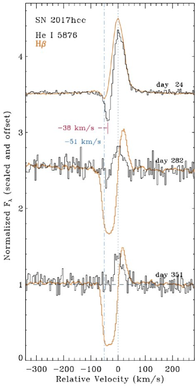
Figure 8: Detail of MIKE echelle spectra on the three epochs showing the narrow component of He i $\lambda$5876 (black) compared to H$\beta$ (orange). Approximate velocities of the early-time narrow absorption trough of H$\beta$ (at $-$51 km s^-1; blue) and He i (at $-$38 km s^-1; magenta) are marked.

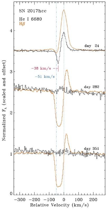
Figure 9: Same as Figure 8, but for He i $\lambda$6680.

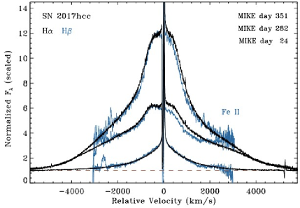
Figure 10: Comparison between the full line profile shapes of H$\alpha$ (black) and H$\beta$ (blue) in the three epochs of echelle spectra. The H$\beta$ strengths have been scaled to match H$\alpha$, to correct for their different line/continuum flux ratio, and so that their shape can be compared directly. For the two later epochs, there appears to be a slight deficit of H$\beta$ flux on the red wing at intermediate velocities. The flux is on a linear scale.

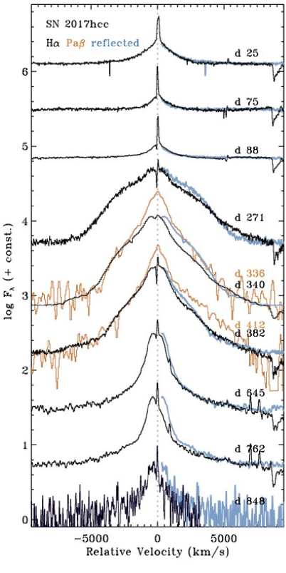
Figure 11: Time series of the H$\alpha$ line profile shape in our moderate-resolution spectra (MMT Bluechannel and Binospec). For each date, the black line is the observed line profile, whereas the blue line shows the blue wing of the emission line reflected across v=0 km s^-1. This is meant to show how the red wing of the line would appear if the line were symmetric. The orange spectra are the infrared Pa$\beta$ line from our MMT/MMIRS spectra on days 336 and 412, for comparison with the H$\alpha$ profile at similar epochs. The Pa$\beta$ profile is expected to suffer less extinction, and its red wing roughly matches the blue reflected wing of H$\alpha$. Pa$\beta$ indicates that significant line flux may be absorbed around zero velocity in optical lines. The flux is on a log scale.

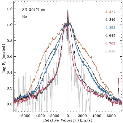
Figure 12: Same as Figure 11, but with the late-time H$\alpha$ profiles plotted on top of one another, scaled arbitrarily to directly compare line shape. Here we only show the late-time profiles after the symmetric Lorentzian scattering profiles no longer dominate the line shape, instead showing the broad component from the SN ejecta and the intermediate-width component from the CDS. The flux is on a log scale.

3 RESULTS

3.1 Na I D and interstellar extinction

The high-resolution MIKE echelle spectra allow a sensitive probe of the interstellar absorption components from the Na i D doublet. The individual D₁ and D₂ lines are easily resolved in the echelle spectrum, and the high resolution allows greater sensitivity to narrow absorption features, compared to moderate-resolution spectra. For examining interstellar absorption, we consider early spectra when the continuum is strongest.

Figure 3 shows the region around Na i D, with the day 24 echelle spectrum (black) compared to the moderate-resolution spectrum taken with MMT one day later (orange). While both spectra have enough resolution to separate the doublet, the absorption features are more clearly defined in the MIKE spectrum. One can see the relatively strong Na i D absorption from the Milky Way interstellar medium (ISM), which here is shifted to shorter wavelengths because we are showing wavelengths corrected to the rest frame of the host galaxy. One can see the weaker Na i D absorption from the ISM in the host galaxy. In the lower resolution spectrum, the Milky Way absorption is barely detected, and the host galaxy absorption is undetected. Figure 3 also shows the strong narrow P Cygni feature of He i $\lambda$5876 and its wings, which will be discussed later.

For the Milky Way absorption component of Na i D, we measure equivalent widths of EW(D₂) = 0.129 ($\pm$0.006) Å, EW(D₁) = 0.085 ($\pm$0.005) Å, and EW(D₂+D₁) = 0.214 ($\pm$0.008) Å. Using the relations from Poznanski et al. (2012), these translate to $E(B-V)$ values of 0.023 mag (D₂), 0.028 mag (D₁), and 0.025 mag (D₁+D₂). As noted by Poznanski et al. (2012), there is a 30-40% systematic uncertainty in the relation for $E(B-V)$. These are in reasonable agreement with the Milky Way line of sight reddening of $E(B-V)$=0.0285 mag adopted earlier (Schlafly & Finkbeiner, 2011).

For the SN 2017hcc host galaxy ISM absorption component of Na i D, we measure smaller equivalent widths of EW(D₂) = 0.026 ($\pm$0.005) Å, EW(D₁) = 0.014 ($\pm$0.004) Å, and EW(D₂+D₁) = 0.039 ($\pm$0.006) Å. Using the relations from Poznanski et al. (2012), these would translate to $E(B-V)$ values of 0.014 mag (D₂), 0.019 mag (D₁), and 0.016 mag (D₁+D₂). A note of caution is warranted here, because these host galaxy EW values we measure are below the range of EW over which the relations from Poznanski et al. (2012) were calibrated, which extend down to 0.05 Å, and there is some indication that data deviate from the fit at the lowest EW values. We therefore regard $E(B-V)$=0.016 mag as an upper limit to the host galaxy reddening for SN 2017hcc, corresponding to $A_{V}$ $\la$ 0.05 mag. This small host reddening and extinction makes no difference in our analysis that concentrates on line profile shapes, but this result may be useful for other studies of the photometry and polarization of SN 2017hcc.

3.2 Broad and intermediate-width components

The line profiles of H$\alpha$ and H$\beta$ are characterized by narrow emission with P Cygni absorption atop a broader emission component. At early times, the broader component has a Lorentzian shape, with a FWHM value of about 2000 km s^-1 or 1600 km s^-1 for H$\alpha$ and H$\beta$, respectively (see Figs. 4 and 5). At later times, however, the broader line shape becomes less symmetric. The line shape at later epochs after day $\sim$100 is clearly not a single Gaussian or Lorentzian shape, but seems to have at least two subcomponents, with an intermediate-width component at velocities below 2000 km s^-1, and a broader component extending out to around 5,000 km s^-1 on the blue and red wings of the line. The line asymmetry permits multiple ways to fit the line shape.

Figure 6 shows two examples of how the same line might be approximated with two Gaussian components. Figure 6a (top) shows an example where the centroids of the Gaussians are permitted to shift, and Figure 6b (bottom) shows Gaussian components that have a center fixed at zero velocity, but allowing red wings to fall below the model.

In Figure 6a, even two broad components with FWHM values of 4000 and 1300 km s^-1, with line centers shifted by $-$200 and $-$40 km s^-1, respectively, are insufficient to give a satisfying fit the detailed line shape. The observed central intermediate-width component is more boxy than the Gaussian, and the broad wings do not match the Gaussian shape well. An additional broad Gaussian would be needed at roughly +3000 km s^-1 to account for a red emission bump in excess of the fit in Figure 6a.

In Figure 6b, the two broad components with FWHM values of 4000 and 1100 km s^-1 and centers at 0 km s^-1 do not fit the line profile either. However, these particular Gaussians are chosen because the blue wing and the far red wing are matched very well. The Gaussian model clearly exceeds the observed flux from $-$500 to +3000 km s^-1, but this is by design — the motivation for allowing this missing flux is that some of the intrinsic line profile may be absorbed at some velocities. The utility of this seemingly poor fit and the “missing” flux will be apparent later.

Overall, spectra at later times (after the Lorentzian profiles transition to broader lines) seem to consistently require at least two separate components in the broader line profile shape. (1) A broad component with FWHM widths of 4000-6000 km s^-1. This is broader and stronger at first (days 100-300), and then narrower and fading at later times (after day 300). The evolution of the relative strength and width of the broad component with time can be seen in Figure 12. (2) An intermediate-width component with a FWHM of 1000-1500 km s^-1 appears after the Lorentzian components fade, and persists until the latest epochs. As described later, we attribute the broad component to emission from the unshocked SN ejecta, and the intermediate-width component to shocked gas in the CDS. This is the typical interpretation of these features in many SNe IIn (Smith, 2017). Whether one prefers the Gaussians offset from zero or the ones that fit the red side of the line poorly depend on the interpretation of the line profile asymmetry.

In any case, the line profile asymmetry is rather mild at day 200-400, but the asymmetry gets more severe at later times, like in the day 762 spectrum seen in Figure 11. Interestingly, there appears to be a significant change from day 645 to day 762. The blue wing of the line is virtually identical at these two epochs, but the red wing changes drastically (examine Figures 11 and 12), with the line becoming much more asymmetric and suppressed on the red side. The likely interpretation of this change is discussed later.

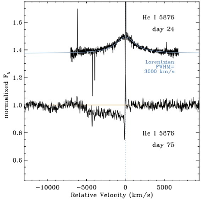
Figure 13: The day 24 MIKE spectrum around He i $\lambda$5876, compared to a Lorentzian line profile (blue) with a FWHM = 3000 km s^-1, and the day 75 MMT spectrum showing the broad P Cygni absorption seen in He i $\lambda$5876. The weak absorption at around $-$10,000 km s^-1 on day 75 could be a fast component of He i, or may be from a different line.

The broader components of He i lines behave differently from Balmer lines. At early times, He i $\lambda$5876 has a broad Lorentzian profile underneath the narrow P Cygni components, which can be seen in Figures 3 and 13. This Lorentzian has a width of 3000 km s^-1, whick is faster/broader than the Balmer lines at the same epoch (this broader width may indicate electron scattering in hotter gas). The broad He i emission is weak and fades during the first 100 days. Interestingly, in our spectra, He i $\lambda$5876 shows the clearest evidence of broad blueshifted P Cygni absorption from fast ejecta during the main peak of the SN. This broad absorption can be seen reaching to almost $-$6,000 km s^-1 in the day 75 spectrum (Figure 13), and probably indicates that we are beginning to directly see the fast SN ejecta at this epoch. (A weaker absorption feature can also be seen at $-$10.000 km s^-1, but this might arise from different line transition.) It is not so unusual to observe fairly strong broad blueshifted absorption from He i $\lambda$5876 in the ejecta of SNe IIn during the main luminosity peak (e.g., Mauerhan et al. 2013; Smith et al. 2014). However, since Balmer lines still show strong Lorentzian profiles that indicate high electron scattering optical depths in the CSM at this same epoch, this suggests that we are able to see the fast SN ejecta because of asymmetric geometry. For instance, we may be looking down on polar regions of the SN ejecta, despite high continuum optical depths in the equatorial CSM.

3.3 Narrow CSM components

Our high-resolution MIKE echelle spectra are particularly useful for investigating the narrow emission and absorption arising from the pre-shock CSM. The narrow CSM lines are well resolved, appearing significantly broader ($\sim$50 km s^-1) than the instrumental resolution of $\la$10 km s^-1.

The narrow components of the three Balmer lines H$\alpha$, H$\beta$, and H$\gamma$ are shown in Figure 7. All three lines show qualitatively similar evolution, with a strong narrow emission and weak P Cygni absorption at the first epoch on day 24, transitioning to much deeper P Cygni absorption and weaker emission at the later two epochs (days 282 and 351).

On day 24, the narrow P Cygni absorption from H$\alpha$ is weak and poorly defined, but the narrow H$\beta$ and H$\gamma$ absorption is more clear. The centroid of the H$\beta$ absorption is found at $-$51 km s^-1 ($\pm$1 km s^-1), indicated by the vertical light blue bar in Figure 7. Interestingly, the speed of the H$\gamma$ absorption is a little slower, at roughly $-$47 km s^-1 ($\pm$1 km s^-1), while the H$\alpha$ absorption (admittedly weak and harder to measure) seems to be at a faster speed of $-$55 km s^-1 ($\pm$2 km s^-1), so there seems to be a march to the red for absorption components going from H$\alpha$ to H$\gamma$. There is a shift in the opposite sense for emission components, with the peak marching slightly to the blue as we go from H$\alpha$ to H$\gamma$. The FWHM of the emission components also gets narrower as we proceed up the Balmer series, with FWHM values of 50 ($\pm$1 km s^-1), 49 ($\pm$1 km s^-1), and 46 ($\pm$1) km s^-1 for H$\alpha$, H$\beta$, and H$\gamma$, respectively. Thus, all three trends (shifts in absorption minimum, peak emission, and FWHM) trace lower outflow velocities for higher order Balmer lines. (We note, however, that the decrease in FWHM may be partly caused by the increase in strength of the P Cygni absorption from H$\alpha$ to H$\gamma$, where the stronger P Cygni features decrease the flux on the blue side of the emission component.)

There is also a change in the centroid of the P Cygni absorption to lower velocities at later times in Balmer lines (Figure 7), but it is not a simple shift of the absorption to slower speeds. Rather, on days 282 and 351, the blue edge of the P Cyg absorption stays roughly the same as in the first epoch, but the absorption gets wider for all three Balmer lines. It therefore appears that the absorption at later times is tracing a larger range in CSM expansion speeds along the line(s) of sight, including additional slowly expanding gas that was not seen in the first epoch, rather than a net shift to lower speeds in the CSM. The widening absorption at later epochs also eats into the emission peak, pushing it further to the red and making it weaker for all three lines.

The narrow CSM components of He i lines show some interesting differences compared to Balmer lines. Figure 8 shows narrow components of He i $\lambda$5876 compared to H$\beta$, while Figure 9 shows the same for He i $\lambda$6680. The day 24 spectra reveal well-defined narrow absorption from He i lines, but it is at a slower outflow speed than Balmer lines. Both He i lines have an absorption minimum at $-$38 ($\pm$1) km s^-1, more than 10 km s^-1 slower than H$\beta$. The He i lines therefore seem to extend the trend of marching to slower speeds at higher excitation and ionization. Unlike the shift at late times in Balmer lines, this is not a widening of the absorption, but a clear shift of the narrow component to slower outflow speeds. Also unlike Balmer lines, He i lines do not develop much deeper and broader absorption at late times, but instead, the absorption gets weaker (there seems to be weak He i $\lambda$5876 absorption at about the same velocity of $-$38 km s^-1 on day 282) or the lines are not detected. There is some lingering emission in He i $\lambda$5876 at both later epochs, and only very weak emission on day 282 for He i $\lambda$6680. The physical significance and interpretation of the CSM emission will be discussed below in Section 4.

3.4 Asymmetry and wavelength dependence

Above in Section 3.2 we noted a mild asymmetry in the H$\alpha$ profile at later epochs, requiring either a slightly blueshifted centroid for Gaussian fits, or a deficit of flux on the red wing compared to symmetric profiles (Figure 6). There is also a subtle wavelength dependence and a time dependence to this asymmetry that we discuss in more detail here.

Figure 10 shows the same MIKE spectra of H$\alpha$ and H$\beta$ that appeared earlier, but here they are plotted together. The day 24 profiles of H$\alpha$ and H$\beta$ are nearly identical, and both are consistent with symmetric Lorentzian profiles. The later spectra on days 282 and 351 show clear differences in the line profile shapes. The blue wings of the lines match quite well at the later two epochs; while we have admittedly scaled the line strengths to overlap on the blue side, it is also true that the shape of the blue wings match for H$\alpha$ and H$\beta$. In contrast, the red sides of the H$\alpha$ and H$\beta$ lines do not match on days 282 and 351, with H$\beta$ showing a clear deficit of emission on the red wing of the intermediate-width component on both dates. The blueshifted asymmetry in the H$\alpha$ profile becomes more pronounced at H$\beta$.

A consistent extension of this trend in the wavelength dependence is seen as we move to the IR. Figure 11 includes a time series of H$\alpha$ line profiles in low-resolution spectra, but it also includes the 1.28 $\mu$m Pa$\beta$ line from our two late epochs of IR spectra taken with MMIRS on the MMT. Comparing H$\alpha$ and Pa$\beta$, it is evident that these profiles have very different shapes. If we match the flux on the blue side of the line profile, then Pa$\beta$ shows an excess in the peak of the intermediate-width component (within $\pm$800 km s^-1) and excess flux over most of the red wing of the line. Interestingly, the excess of Pa$\beta$ over H$\alpha$ in Figure 11 is quite similar to the excess of a symmetric Gaussian model above the observed H$\alpha$ profile shown in Figure 6b. Overall, we conclude that there is a subtle but clear wavelength dependence in the H emission lines, such that lines at shorter wavelengths have a more pronounced blueshift.

The asymmetry in emission profiles is also time dependent. Figure 11 also shows the blue wing of the line reflected across to the red side of the profile (in light blue) in order to illustrate deviations from a symmetric profile shape. We can characterize the evolution in three main phases:

1. Early times (up to day 100) show little asymmetry, with a narrow component atop broader symmetric Lorenztian profiles. Small deviations from symmetry are that days 75 and 88 seem to show some excess flux on the red side (i.e. in the opposite sense of the blueshifted asymmetry at later times). This might indicate some broad P Cyg absorption that suppresses the blue wing of H$\alpha$ (recall that broad blueshifted He i is clearly seen at this epoch) or a slight redward shift in the centroid of the Lorentzian profile.

2. Intermediate phases (roughly days 200-400 sampled by our spectra) show both a broad component and an intermediate-width component. These epochs exhibit a significant deficit of flux on the red side of the line in both the intermediate-width and broad components, although the deviation from symmetry changes from one epoch to the next. This asymmetry is wavelength dependent, with more pronounced blueshift at shorter wavelengths.

3. Late phases (after day 500-600 or so) are dominatedf by an intermediate-width component, with the broad component having faded substantially or become narrower so that it is blended with the intermediate-width component. During this late phase, the intermediate-width component shows a clear blueshifted asymmetry that becomes more pronounced with time. Note the discrepancy between the observed red wing compared to a reflected blue wing, moving from day 645 to 762 (Figure 11).

The profile in the day 762 spectrum has a striking asymmetry, with a peak shifted to about $-$350 km s^-1. This profile cannot be fit by a symmetric Gaussian or Lorentzian that has a shifted centroid. Rather, the peak is skewed to the blue, missing emission at low redshifted velocities, though the broader wings are almost symmetric.

The change from phase 2 to 3 is even more evident in Figure 12, where we overplot the H$\alpha$ profiles at various times (excluding the early Lorentzian phase). Here we see that the broad component decreases in strength and/or width from day 271 to days 340 and 382, and then the broad component is gone by days 645, 762, and 848, while the width of the intermediate component changes very little except for the increase in blueshifted asymmetry of the peak.

4 DISCUSSION

In the discussion below, numbered days refer to days since the inferred explosion date of 2017 Oct 1 (see above). On this scale, for reference, the time of peak visual light was around day 40-45, and the peak bolometric luminosity was around day 30 (Prieto et al., 2017).

4.1 Overall Line-profile Evolution

SN 2017hcc exhibits the classic evolution of line profile shapes that is common in strongly interacting SNe IIn, which transition from symmetric Lorentzian profiles at early times (before and during peak), to irregular, broader, and asymmetric shapes at late times well after peak. This is understood as a shift from narrow CSM lines broadened by electron scattering to emission lines formed in the post-shock CDS (Smith, 2017; Smith et al., 2008b; Dessart et al., 2015).

The early profiles are characterized by a very narrow emission-line core (about $\sim$50 km s^-1`) that also has a narrow P Cygni absorption component. These early profiles have broad wings that follow a symmetric Lorentzian shape, due to incoherent electron scattering of narrow emission from pre-shock gas (Chugai, 2001, 2018; Smith et al., 2008b, 2010a, 2012a; Smith, 2017). At these times, the narrow line width traces the pre-SN mass-loss speed, whereas the line wings are caused by thermal broadening and are not due to expansion speeds. This indicates that at these early times (usually up to and including the time of peak luminosity), the continuum photosphere is in the CSM ahead of the shock, hiding emission from the CDS and SN ejecta. By day 65, however, we may begin to see the fast SN ejecta directly via broad P Cygni absorption in He i $\lambda$5876 (Figure 13). Seeing this broad absorption while still seeing Lorentzian profiles in Balmer lines may require asymmetry in the CSM.

At later times, however, emission from the fast SN ejecta and CDS become visible after optical depths drop and the photosphere recedes (in mass), and as the shock overtakes the photosphere. For SN 2017hcc, this transition took place sometime during a gap in our spectral coverage between days 92 and 271, missed because SN 2017hcc was behind the Sun. From day 271 onward, spectra reveal a more complex line profile shape in H$\alpha$ with at least two broader components (Figure 6). These two include a broad emission component with FWHM = 4000 km s^-1 that we interpret as tracing the fast, unshocked SN ejecta, as well as an intermediate-width component with FWHM = 1100 km s^-1, which we interpret as emission from the post-shock gas in the CDS. Narrow emission and P Cyg absorption from the pre-shock CSM persist to late times as well.

This transition is typically seen in SNe IIn (Smith et al., 2008b; Smith, 2017), and essential properties of the transition are reproduced in radiative transfer simulations of SNe IIn (Dessart et al., 2015). These simulations affirm the interpretation of electron scattering in the CSM at early times and emission from post-shock gas at later times.

An interesting aspect of the H$\alpha$ line-profile evolution in SN 2017hcc is the clear identification of a broad emission component reaching $\pm$6,000 km s^-1 that we attribute to the fast SN ejecta (Figures 6b, 11, and 12). After day $\sim$200, this broad component has comparable strength to the intermediate-width component from the post-shock CDS and it dominates the appearance of the H$\alpha$ line. As time progresses, the broad component declines in strength and width and disappears by day 752, whereas the intermediate-width component persists at all late epochs with a roughly constant width (ignoring affects associated with asymmetric absorption; see below). This different time evolution confirms that the two emission components have a different origin from one another. Seeing strong emission from the freely expanding SN ejecta is rare in SLSNe IIn, where continuum optical depths often hide the emission from underlying ejecta, or where stronger emission from the intermediate-width component dominates the lines. For example, the broader component from SN ejecta was absent or much weaker in day$>$200 spectra of SN 2010jl (Smith et al., 2012a; Gall et al., 2014; Fransson et al., 2014), and SN 2006tf showed only weak H$\alpha$ emission and faint O i and He i absorption at fast blueshifts (Smith et al., 2008b). Since we see the SN ejecta more clearly in SN 2017hcc, we may be viewing from a different orientation (looking from the poles, for example).

Identifying the broad emission with the SN ejecta also has important implications for interpreting the asymmetry in SN 2017hcc’s line profiles discussed below, and for its high observed continuum polarization. The broad emission component of H$\alpha$ shows only mild asymmetry (Figure 12), with a small portion of its red wing depressed compared to a symmetric profile (Figure 6). Importantly, though, the red and blue wings of the broad component are symmetric at velocities faster than $\pm$3000 km s^-1. Moreover, the line profile of the infrared line Pa$\beta$, where any dust absorption should be less influential than in the optical, is quite symmetric as well (Figure 11). This means that the intrinsic emission-line profile from the fast SN ejecta is symmetric, which has two critical implications: (1) High continuum optical depths associated with the SN photosphere are not blocking the receding side of the explosion at late times, because the broad lines are symmetric at the highest velocities. Therefore, something else is causing the blueshifted line asymmetry in late-time spectra. (2) The symmetric emission suggests that the underlying SN explosion itself was not highly aspherical. This, in turn, would mean that faster or denser SN ejecta in a particular direction (i.e. a lopsided explosion) are not causing stronger CSM interaction in a particular direction in SN 2017hcc, and asymmetry in the underlying SN explosion is probably not responsible for SN 2017hcc’s high polarization. Instead, the polarization is likely related to aspherical CSM, and the blueshifted line profiles are likely caused by selective absorption, discussed later.

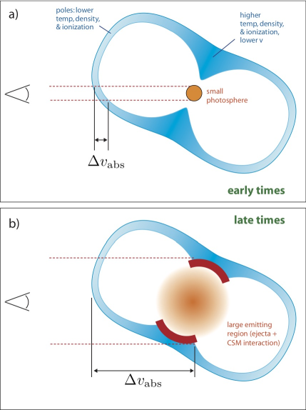
Figure 14: Sketch illustrating how a hypothetical CSM geometry may explain the observed behavior of narrow emission and absorption lines in SN 2017hcc. Panel (a) represents early times within the first $\sim$100 days, and panel (b) shows later times after day 200. The same bipolar CSM configuration (blue) is shown in both panels, where the structure is meant to symbolize latitude-dependent outflow velocity, rather than physical size and radius (although these are related if the CSM was made by an episodic mass ejection). The main difference in the two panels is the change in the emitting source of continuum and broad/intermediate-width line emission: (a) at early times, the emitting source (orange) is the SN photosphere, which still has a relatively small radius. This light passes through a small section of the polar CSM, resulting in a narrow range of absorbed velocities ($\Delta v_{\rm abs}$). (b) at later times, the ejecta and shock have expanded, and most of the luminosity is generated in a more extended CSM interaction shock (dark red) and in the expanded SN ejecta (orange gradient). This light passes through a much larger section of the CSM, yielding a broader range of $\Delta v_{\rm abs}$. A hypothetical Earth-based observer is at left. This observer sees narrow emission from all parts of the CSM shell, but only sees absorption generated along the line of sight to the continuum or broad-line emitting regions.

4.2 Narrow components and the pre-shock CSM

4.2.1 The narrow component at high resolution

A novel aspect of this study is that we obtained three epochs of high-resolution echelle spectra, which provides a unique view of the narrow-line emission from slowly expanding CSM. Only a few examples of high-resolution echelle spectra for SNe IIn have been published, including SN 1998S on day 1 (Shivvers et al., 2015), SN 1997ab a few months after explosion (Salamanca et al., 1998), SN 1997eg on roughly day 200 (Salamanca et al., 2002), and SN 2005gj (a Type Ia/IIn hybrid) on days 86 and 374 (Trundle et al., 2008). These had inferred progenitor wind speeds deduced from narrow lines of 40 km s^-1 (SN 1998S), 90 km s^-1 (SN 1997ab), 160 km s^-1 (SN 1997eg) and 60-130 km s^-1 (SN 2005gj).

It is clear that with CSM expansion velocities of only 40-50 km s^-1 in the case of SN 2017hcc, the CSM emission and absorption are completely washed out in most low-resolution optical spectra that are usually used for observing SNe (typically $R$=$\lambda$/$\Delta\lambda$ of 300-1000, or up to 300 km s^-1 resolution for full broad wavelength range optical spectra). The narrow line profiles are underresolved even in moderate-resolution spectra like those we typically obtain using a 1200 lpm grating with Bluechannel on the MMT (Andrews et al., in prep.), or spectra obtained with X-shooter on the VLT (typically $R$ of 4000-1000 or 30-80 km/s). Examples of the narrow components in echelle spectra as compared to moderate resolution MMT ($R\sim$4000) spectra are shown in Figures 3, 4, and 5. In the first epoch especially, the narrow P Cyg absorption is lost in moderate-resolution spectra.

Based on the results for narrow lines discussed above, we summarize key observed properties for SN 2017hcc that any model for its CSM should explain:

1. Early times show relatively weak blueshifted absorption with a narrow range of speeds centered around 40-50 km s^-1. The blue edge of the absorption is around $-$60 or $-$70 km s^-1 (different values for different lines).

2. At later times, the blue edge velocity remains about the same, but the range of absorbed speeds is wider, extending to slower speeds, and the absorption is deeper.

3. By day 75, we begin to see the fast SN ejecta, even though the optical depths in the CSM remain high. This requires non-spherical geometry.

4. Deeper Balmer line absorption at late times reaches down to $\sim$20% of the continuum, but this “continuum” is mostly the underlying broad components of the same emission line. This means that the absorption source is along our line of sight to both the photosphere and the broad components. The continuum luminosity and intermediate-width component may arise in the same CSM interaction region.

5. The narrow emission (especially its red wing) stays roughly the same at all epochs, and has a velocity width similar to the early absorption speed around 40-50 km s^-1. This indicates that the asymmetry in CSM velocity is fairly mild, and that the CSM speed ahead of the shock remains similar over a range of radii as the shock moves out through it, regardless of the changing luminosity of the SN. This, in turn, suggests that any non-sphericity in the CSM geometry is probably axisymmetric rather than one-sided.

6. The higher excitation and higher ionization lines, which are normally formed deeper in a stellar wind or closer to the shock in a SN, have slightly lower speeds (i.e. 38 km s^-1 in He i vs. 55 km s^-1 in H$\alpha$, and slightly decreasing speeds in higher-order Balmer lines). This same trend was also observed in narrow components of SN 2005gj (Trundle et al., 2008). We are not aware of any other SN IIn where this has been seen in high-resolution data. Interestingly, the opposite was seen in spectra of SN 1998S, where the narrow cores of higher-ionization lines were systematically broader than lower-ionization lines (Shivvers et al., 2015). This difference could be partly due to the fact that the high-resolution spectrum of SN 1998S was taken within 1 day of explosion, which still included emission from the inner acceleration zone of the progenitor wind.

One conjecture that is immediately apparent from this list is that a single-speed, constant velocity spherical wind cannot reproduce these properties. Instead, some more complicated geometry or time dependence is needed.

4.2.2 Axisymmetric geometry in the CSM

Figure 14 shows a sketch that illustrates how a hypothetical CSM geometry might account for the observed behavior of narrow lines seen in SN 2017hcc. While this is admittedly not a unique explanation, it does account for several traits that a spherical wind cannot. The basic idea represented in this figure is that the SN explodes inside a CSM shell that has a bipolar configuration, borrowing from nebulae often seen around LBVs like $\eta$ Car (Smith, 2006; Smith et al., 2018b), except with much slower expansion speeds than $\eta$ Car. This slow CSM nebula (tinted blue in Figure 14), viewed by an Earth-based observer at some intermediate latitude, has higher velocities, larger radii, and a larger inner cavity along the poles, and it has higher densities and lower velocities in the equator. As in the case of $\eta$ Car, such a structure might arise from an LBV-like eruption in a massive binary interaction or merger event (Smith et al., 2018a). The emission component of the narrow lines arises in the portions of the CSM that are not along the line-of-sight (again, the blue region in Figure 14, and this emission retains approximately the same velocity at all times because it is the integrated emission from most of the CSM.

The key point conveyed in Figure 14 is that the underlying source of luminosity (tinted orange/red) is expanding with time, causing the emitted radiation to traverse different paths (and hence different velocity ranges) through the asymmetric CSM. At early times during the SN peak (Figure 14a), the emitting radius is small compared to the size of the nebula, and so the continuum radiation traces a pencil beam through only a small section of the CSM. In this case, it passes through only a small section of the thin polar cap, yielding weak blueshifted absorption near the maximum speed with only a narrow range of velocity (small $\Delta v_{\rm abs}$). At late times (Figure 14b; past day 200 when the continuum luminosity has dropped), the emitting source that is absorbed becomes more complicated. The continuum luminosity has mostly faded, and the photons being absorbed by the CSM are now the broad component from the freely expanding SN ejecta (orange gradient) as well as the intermediate-width component from the strong CSM interaction, which may be dominated by emission from the post-shock CDS in the dense equatorial CSM (red arcs). This broad line emission passes through a much larger sample of the CSM and traces a wider range of speeds (hence, larger observed $\Delta v_{\rm abs}$). In this case, the blue absorption edge is still about the same, corresponding to the polar speed – but absorption now occurs at speeds all the way to zero, because some of the absorbing CSM is moving transversely in the plane of the sky and has no Doppler shift. The absorption is also deeper at these later times, because most of the source photons pass through denser material and longer path lengths through the low-latitude portions of the CSM. Thus, this CSM configuration meets the first 4 requirements listed above.

At some epoch intermediate between Figures 14a and 14b, a transition occurs. The photosphere is outside the shock and obscures the CDS and SN ejecta at early times, but eventually the CSM interaction at the equator becomes dominant, and the optical depths through polar regions thin first. At this point, we may begin to see SN ejecta directly down the poles. This may explain the broad blueshifted He i $\lambda$5876 absorption on day 75 (Figure 13), while we can still see Lorentzian profiles arising from electron scattering of H emission lines in equatorial CSM regions.

The sixth requirement above, that slower velocities are seen in higher ionization lines like He i, or higher order Balmer lines like H$\gamma$, may be achieved in this configuration as follows. These lines will prefer regions of higher temperature and ionization. In the configuration shown in Figure 14, these are most likely to be found closer to the source of SN luminosity and closer to the strongest shock interaction - i.e., in the regions of the pinched waist near the equator where the expansion velocities are slower and directed out of our line of sight. Lower velocities at smaller radii arise naturally in CSM created in episodic mass loss, as opposed to a steady wind. Thus, a bipolar configuration may naturally satisfy the requirement of lower velocities for higher excitation. This is harder to imagine in a spherical CSM configuration. At late times, the He i lines may weaken significantly, as observed (Figures 8 and 9), for a few reasons: this may happen because the inner equatorial CSM has been swept up, or simply because the SN’s luminosity has dropped and the shock speed has slowed, allowing the remaining pre-shock gas to cool and He to be mostly neutral.

4.2.3 Radiative acceleration or geometry?

The sixth requirement above (slower speeds for higher excitation) also has important consequences regarding any acceleration of pre-shock CSM by the radiation from the SN itself (Chugai, 2019). Radiative acceleration of pre-shock CSM has sometimes been invoked to account for blueshifted line profiles seen in some SNe IIn, like SN 2010jl (Fransson et al., 2014; Zhang et al., 2012). However, this effect should be most important for the peak-luminosity phase of the SN, whereas the blueshifted line profiles persist to late times in most SNe IIn. Moreover, radiative transfer simulations for SN 2010jl (Dessart et al., 2015) indicate that radiative acceleration cannot reproduce the observed blueshift.

For SN 2017hcc, the observed velocity patterns suggest that any effect of pre-shock acceleration of the CSM is unimportant. Radiation from the shock could, in principle, propagate upstream so that photon momentum from the tremendous SN luminosity could radiatively accelerate the unshocked CSM, just as stellar luminosity radiatively accelerates winds in massive stars. If this happens in CSM with high optical depth, as required in SNe IIn, then we expect the strongest pre-shock acceleration in upstream regions that are close to the shock, tracing regions of higher temperature and ionization, and milder or minimal acceleration at larger and cooler radii in the CSM. Radiative transfer simulations confirm that H$\alpha$ arises at larger radii than lines like H$\gamma$ or He i, which come from a similar deeper region (e.g., Shivvers et al. 2015; Dessart et al. 2015). So in the case of radiative acceleration by a SN IIn, one expects higher outflow speeds in He i lines or in H$\gamma$ as compared to H$\alpha$, because these lines are closer to the shock. This effect was indeed seen in SN 1998S (Shivvers et al., 2015). SN 2017hcc shows the opposite trend, however, with lower outflow speeds in He i and H$\gamma$. This means that the observed differences in speed are not tracing acceleration of the unshocked CSM by radiation from the SN, and that any radiative acceleration of pre-shock CSM is smaller than the 10 km s^-1 difference in these lines. Radiative acceleration of the pre-shock CSM must also, therefore, play no role in the blueshifted asymmetry seen in emission lines at late times. Instead, the likely explanation for the slower outflow speeds in He i and H$\gamma$ may be geometric, as noted earlier.

The bipolar CSM geometry invoked in Figure 14 is hardly unusual; in fact, axisymmetric CSM tends to be the norm rather than the exception among massive star nebulae (Nota et al., 1995; Smith, 2014, 2017), probably due to the pervasiveness of binary interaction in massive star evolution (Sana et al., 2012; Moe & Di Stefano, 2017). Overall, the CSM expansion around SN 2017hcc is fairly slow, with the bulk speed of around 40-50 km s^-1 and a blue edge to the P Cygni absorption at only $-$70 km s^-1. Because the absorption speed seen at early times is comparable to the emission width, and because the blue edge stays the same throughout its evolution, it is likely that we view SN 2017hcc along a sightline corresponding to a mid-latiutude or high latitude (say within 45^∘ or so of the symmetry axis). This is different from SN 2010jl, where the P Cyg absorption speed is slower than the narrow emission width (Smith et al., 2011a), suggesting a view from low latitudes.

Although bipolar nebulae are common around LBVs (Nota et al., 1995), most notably around $\eta$ Carinae (Smith, 2006), the expansion speed of the CSM around SN 2017hcc is relatively slow compared to typical LBV winds and nebular expansion speeds of $\ga$100 km s^-1 (Smith, 2014). However, because of their bipolar geometry, some LBVs exhibit a wide range of outflow speeds in a single object; for example, although $\eta$ Car has a wind speed of 500 km s^-1 (Smith et al., 2003; Hillier et al., 2006) and the poles of its nebula are expanding at 650 km s^-1 (Smith, 2006), it has much slower speeds of only 40 km s^-1 in its equatorial regions (Zethson et al., 1999; Smith, 2006; Smith et al., 2018b). There are also several well-studied blue supergiants that have very slow (10-40 km s^-1; much slower than their stellar winds) expansion in their resolved equatorial ring nebulae. These include Sher 25 (Brandner et al., 1997), SBW1 (Smith et al., 2013), NaSt1 (Mauerhan et al., 2015), the massive eclipsing binary RY Scuti (Smith et al., 2002, 2011b), HD 168625 (Smith, 2007), and of course the progenitor of SN 1987A (Meaburn et al., 1995; Crotts & Heathcote, 2000). These slow disks are thought to arise from binary interaction episodes, allowing outflows much slower than their raditively driven winds. The class of B[e] supergiants are also blue supergiants that are inferred to have slow, dense, equatorial outflows (Zickgraf, 2006; Kraus, 2019). While the CSM around SN 2017hcc is expanding faster than the winds of normal RSGs (typically 10-20 km s^-1), there is a subset of extreme, high-luminosity RSGs with faster winds and high mass-loss rates, some of which also have asymmetric or axisymmetric structures in their CSM. One pertinent example is VY CMa, which has mildly bipolar geometry, with the bulk outflow at 35-40 km/s, but with some faster features up to 70 km/s (Smith, 2004; Smith et al., 2009a; Decin et al., 2016). Another extreme RSG with bipolar geometry seen in water masers is VX Sgr (Berulis et al., 1999; Pashchenko et al., 2006).

Similar bipolar/disk geometries, viewed from different orintation angles, have been invoked for several other SNe with strong interaction, including SN 2009ip (Mauerhan et al., 2014; Smith, 2014), SN 2010jl (Andrews et al., 2011; Smith et al., 2011a; Gall et al., 2014; Fransson et al., 2014; Dessart et al., 2015), SN 2007rt (Trundle et al., 2009), PTF11iqb (Smith et al., 2015), SN 2014ab (Bilinski et al., 2020), SN 2010jp (Smith et al., 2012b), iPTF14hls (Andrews & Smith, 2018), SN 2013L (Andrews et al., 2017), SN 2013ej (Mauerhan et al., 2017b), SN 1998S (Leonard et al., 2000), and SN 1997eg (Hoffman et al., 2008), among others. Common indications of bipolar geometry and slow disks around SNe IIn might hint at a common mechansim related to pre-SN binary interaction (Smith & Arnett, 2014).

4.3 Pre-SN Mass Loss

Armed with reliable estimates of the speeds of the CSM and CDS, and the observed SN luminosity, we can make several rough estimates of the pre-SN mass loss. The observed narrow CSM lines indicate an outflow speed of 40-50 km s^-1, so we take an average velocity for the pre-SN mass loss of $V_{\rm CSM}$=45 km s^-1. The measured FWHM of the intermediate-width component of H$\alpha$, emitted by the CDS, is 1100 km s^-1. We multiply this radial velocity by $\sqrt{2}$ to account for the expansion direction predominantly away from our line of sight (see Figure 14), taking $V_{\rm CDS}$=1600 km s^-1.

The luminosity generated by CSM interaction (see Smith 2017 for a review) is given by

$$L=\frac{1}{2}wV_{\rm CDS}^{3}$$ (1)

where $w$ = $4\pi R^{2}\rho$ = $\dot{M}/V_{\rm CSM}$ is the wind density parameter. Here, $L$ is the total bolometric luminosity generated by CSM interaction, which includes line emission and continuum across all wavelengths. The observed UV/optical/IR continuum luminosity is a lower limit for this, but during the main peak of the SN when the CSM interaction shock is below the photosphere that resides in the optically thick CSM, the optical luminosity is a good proxy for $L$. At later times when the material becomes more optically thin and the visual-wavelength luminosity drops, an increasing fraction of the luminosity may escape as line emission and X-rays. (The value of $L$ may also change as the SN evolves and the shock decelerates or runs into varying density CSM.) The progenitor’s mass-loss rate can be expressed as

$$\dot{M}_{\rm CSM}=2L\frac{V_{\rm CSM}}{V_{\rm CDS}^{3}}$$ (2)

where this is likely a conservative value if $L$ is derived from the visual-wavelength continuum luminosity, which is a lower limit to the true bolometric $L$. Again, the pre-SN mass-loss rate was eruptive and episodic, so $\dot{M}_{\rm CSM}$ may not have been sustained for very long, and only represents the density of the CSM into which the SN shock expands during the main light curve peak.

As noted in the introduction, SN 2017hcc had a peak $V$ absolute magnitude of about $-$20.7 mag, which translates to about 1.6$\times$10¹⁰ $L_{\odot}$ or roughly 6.5$\times$10⁴³ erg s^-1 with no bolometric correction. With such a high luminosity, it is unlikey that the underlying SN ejecta radiation contributes significantly to the total luminosity, so we assume that CSM interaction dominates the emergent luminosity. This is the peak luminosity, so we adopt $L\simeq 4\times 10^{43}$ erg s^-1 as a rough average for $L$ over the first $\sim$100 days. Thus, with the values $V_{\rm CSM}$ = 45 km s^-1 and $V_{\rm CDS}$=1600 km s^-1 adopted above, the CSM required to power the main peak of SN 2017hcc through CSM interaction would have a wind density parameter of $W$=2$\times$10¹⁹ g cm^-1, corresponding to an average mass-loss rate of 8.8$\times$10²⁵ g s^-1 or $\sim$1.4 $M_{\odot}$ yr^-1. Including a bolometric correction or some efficiency factor for converting kinetic energy to radiation would raise the CSM mass, so our estimate of the mass-loss rate can be considered conservative. Of course, if the CSM is aspherical, then the true wind density parameter is higher than quoted above, but occupies only a portion of the solid angle encountered by the SN ejecta.

Since we do not detect significant changes in the CSM speed as the SN evolves, this may have been a constant velocity but very short duration wind. The time period preceding explosion over which this wind was active can be estimated as $t$ = $t_{\rm obs}$ $\times$ ($V_{\rm CDS}/V_{\rm CSM}$). The episodic wind must have operated for about 6-12 years pre-explosion in order to create the CSM that powered SN 2017hcc for the first 100-200 days. Thus, the progenitor of SN 2017hcc shed at least 8-16 $M_{\odot}$ in the decade before it died. This is comparable to estimated values of mass ejected in the decade or so before explosion for other well-studied SLSNe like SN 2006gy, SN 2006tf, and SN 2010jl (Smith et al., 2007, 2008b, 2010b; Fransson et al., 2014; Woosley et al., 2007). Based on the late-time interaction that continued well after the main luminosity peak, the progenitor of SN 2017hcc probably shed mass at a somewhat lower rate for many decades before that.

4.4 Blueshift and Post-Shock Dust Formation

SN 2017hcc shows the progressively increasing blueshift in its emission-line profiles that is common in SNe IIn. There have been four different suggestions for the potential origin of the systematic blueshift seen in SNe IIn, discussed in the next four subsections. The only one that is a viable explanation in the case of SN 2017hcc is the hypothesis of post-shock and/or ejecta dust formation.

4.4.1 Radiatively accelerated CSM

Slow pre-shock CSM could be accelerated by the tremendous luminosity in a SLSN IIn, and with high optical depths in the CSM, the narrow CSM emission lines could be broadened by electron scattering to have intermediate-width Lorentzian line profiles with a blueshifted centroid. This was proposed to explain the strongly blueshifted line profiles in SN 2010jl (Fransson et al., 2014). While the resulting line shape is a symmetric Lorentzian profile, the blueshifted centroid requires a large acceleration, and reqires that we cannot see the redshifted CSM because it is blocked by the SN photosphere, or that the highly asymmetric CSM is mostly on our side of the SN. There are several problems in reconciling this idea with observed properties of SNe IIn:

(1) Since the Lorentzian wings originate as narrow-line photons that are scattered and broadened by thermal electrons, the Lorentzian profile should have the same centroid as the narrow emission, but the observed narrow component is usually not blueshifted and remains narrow even though the center of the Lorentzian is blueshifted. This is the case for both SN 2017hcc and SN 2010jl.

(2) The blueshift is small or absent at early times and becomes progressively more pronounced at later times, but the opposite is expected from this mechanism. The strongest pre-shock acceleration should occur when the SN luminosity is highest (Dessart et al., 2015). In SN 2017hcc, the narrow lines with Lorentzian wings are symmetric and centered at zero velocity for the first $\sim$200 days as the luminosity rises to peak and then falls.

(3) The expected amount of radiative acceleration is much smaller than the observed shift (Dessart et al., 2015). Moroever, in SN 2017hcc, the constant narrow emission components and constant blue edges of the P Cyg absorption confirm very minimal (if any) pre-shock acceleration of the CSM (less than 10 km s^-1), even though the peak of the intermediate-width component becomes blueshifted by as much as 300-500 km s^-1, similar to SN 2010jl.

(4) The net blueshift of the intermediate-width component persists to very late times, but as continuum optical depth drops, the ability of electron scattering to create broad Lorentzian wings also drops. Lines should become narrower and symmetric as the continuum optical depth goes away, and we should see the far side of the CSM. The opposite is observed: the blueshift becomes progressively stronger as the continuum fades.

(5) Electron scattering predicts no wavelength dependence, so we should observe the same blueshift in all lines (except perhaps for lines of different excitation levels, where as noted above, we might expect higher speeds for higher excitation closer to the shock). Observations indicate, however, that the blueshift is wavelength dependent. As noted above, the profiles of H$\beta$, H$\alpha$, and Pa$\beta$ in SN 2017hcc indicate that the lines become progressively more asymmetric at shorter wavelengths, inconsistent with a cause of the blueshift being the result of wavelength-indepenedent electron scattering. A similar wavelength-dependence was seen in SN 2010jl (Smith et al., 2012a; Gall et al., 2014).

So in summary, although radiative forces may produce some acceleration of CSM, it cannot dominate the expansion of the CSM for reasons noted here and in Section 4.2.3.

4.4.2 Continuum photosphere blocks redshifted side of CDS

Occultation by the continuum photosphere of the SN could block emission from ejecta or CSM interaction regions arising on the redshifted side of the SN (Smith et al., 2012a). Dessart et al. (2015) presented radiative transfer simulations that showed this effect could produce a blueshifted emission bump in line profiles of SLSNe IIn, once the photosphere recedes from the pre-shock CSM and direct emission from the post-shock CDS is revealed. As with the previous mechanism, however, this requires high continuum optical depths, so this effect should be strongest at relatively early times, and the lines should become symmetric when the photosphere recedes and the continuum luminosity fades (Smith et al., 2012a; Dessart et al., 2015). However, in most SNe IIn exhibiting blueshifted lines, including SN 2017hcc and SN 2010jl, the opposite is seen. The blueshifted lines persist and even become increasingly blueshifted at late times well after the continuum luminosity has dropped by many magnitudes, as noted in the introduction. In SN 2017hcc, we see the most pronounced blueshift in the intermediate-width component after day $\sim$700. Also, because it arises from occultation by the electron scattering photosphere, this mechanism again predicts no wavelength dependence, clearly contradicted by observations.

4.4.3 One-sided CSM or explosion

In principle, a Type IIn event might show a blueshifted profile shape if there is stronger CSM interaction occuring on the near side of the SN, either because of a non-axisymmetric density distribution in the CSM (with higher densities or smaller radii on our side), or because the explosion was asymmetric with faster or denser SN ejecta aimed preferentially at us. Although one expects axisymmetric CSM from rotating stars and binaries, one-sided CSM might not necessarily be so unusual. Events like mergers or grazing collisions at periastron in eccentric binaries might send a spray of CSM in one preferred direction, as in the outer ejecta around $\eta$ Car (Kiminki et al., 2016; Smith et al., 2018a). Some SNe IIn do show signs of significant non-axisymmetric CSM and SN ejecta (Bilinski et al., 2018). It is, of course, statistically unlikely that one-sided CSM could lead SNe IIn to show a preference for blueshifted lines, but non-axisymmetric CSM may nevertheless be important for individual objects. However, if the CSM is one-sided or the explosion is lopsided, observational clues may indicate this.

For the specific case of SN 2017hcc, one-sided CSM or a lopsided explosion is ruled out because the narrow and broader components of the line profiles are symmetric at early times (excluding blushifted P Cyg absorption of course), and their continued evolution is consistent with an axisymmetric explosion and CSM. The intermediate-width components of H$\beta$ and H$\alpha$ are nearly symmetric during days 200-400, displaying only subtle blueshifted asymmetry. Importantly, there is no sign of asymmetry in the Pa$\beta$ profile during this time, indicating that the intrinsic line profile is symmetric. But then at later times, the blueshifted asymmetry grows even though the blue wing of the line profile stays the same. This behavior cannot be due to significantly one-sided CSM. Also, even though the core of the line becomes asymmetric and blueshifted, Figures 6 and 11 show that the high-velocity wings of H$\alpha$ (beyond $\pm$3,000 km s^-1) are symmetric. This symmetry at high velocity indicates that there is no significant front/back asymmetry in the fast SN ejecta, and that we can see direct emission from the far redshifted side of the SN ejecta (this latter point is important considering the location of the dust, see below). Finally, this mechanism (which depends on true asymmetry in the gas density) predicts no systematic wavelength dependence for the blueshift, contrary to observations.

There are certain patterns in line profile evolution that one would expect with one-sided CSM or lopsided explosions. For example, if there were high-mass CSM concentrated mostly on the near side of a SN (producing a blueshift in emission from the post-shock CDS), then we would expect to see some corresponding and opposite asymmetry in the broader component from the ejecta; namely, in this case the fast SN ejecta on the blue side should hit the shock sooner and the remaining unshocked ejecta should have slower velocities, whereas the red side of the SN ejecta could expand less impeded, allowing us to see a broader red wing in the SN ejecta. This is not seen in SN 2017hcc, although precisely this behavior was seen in SN 2012ab (Bilinski et al., 2018).

Thus, while we see good evidence for axisymmetry in the CSM of SN 2017hcc as noted earlier, there is no evidence for a one-sided CSM density distribution or a significantly lopsided explosion that might yield a net blueshift.

4.4.4 Dust formation

The formation or regrowth of dust grains is the clearly favored explanation for the blueshift of line profiles observed in SN 2017hcc because it self-consistently explains at least four properties that cannot be reconciled with the previous three mechanisms: (1) extinction by dust within the line-emitting gas is the only mechanism consistent with the observed wavelength dependence, where H lines at shorter wavelengths (i.e. H$\beta$ even more so than H$\alpha$) show a stronger deficit of flux on their redshifted portions than those at longer wavelengths (Pa$\beta$), (2) increased extinction from dust would explain why the blue wings of the line profiles remain constant even as their profile shapes become more blueshifted, because dust can only absorb redshifted emission in the line but does not influence the blue side of the line), (3) the gradual formation and buildup of dust as the gas expands and cools is consistent with the fact that the observed asymmetry increases with time as the SN fades, and (4) once dust forms in the post-shock gas, it continues to cause extinction of the redshifted line emission from receding material; this explains why the blueshift persists to very late times, long after the continuum luminosity has faded and the continuum optical depths have dropped. The fact that line profiles begin symmetric and become progressively more blueshifted with time points to dust formation within axisymmetric material.

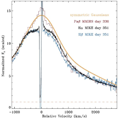
Figure 15: The same day 351 H$\alpha$ and H$\beta$ profiles from Figure 10, but including the 2-Gaussian model (orange) from Figure 6b and the day 336 Pa$\beta$ profile (red histogram) from Figure 11. The plotted velocity range zooms-in on the regions where dust influences the line profile. The Gaussian model is meant to approximate the true intrinsic line profile shape before absorption by dust.

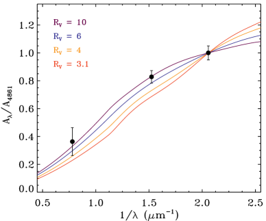
Figure 16: Relative extinction derived from emission line profiles of Pa$\beta$, H$\alpha$, and H$\beta$, normalized to H$\beta$, compared to extinction laws from Cardelli et al. (1989) for various values of $R_{V}$=$A_{V}/E(B-V)$.

SN 2017hcc’s asymmetry in line profiles is admittedly more subtle than in SN 2010jl, but the wavelength dependence is quantifiable. Figure 15 compares the profiles of H$\beta$, H$\alpha$, and Pa$\beta$ scaled to match the blue wings. On the red side of the peak, H$\beta$ is missing only about 3-4% of the flux as compared to H$\alpha$. However, the difference between Pa$\beta$ and either H$\alpha$ or H$\beta$ is more striking, with Pa$\beta$ showing only a mild blueshift (with the caveat that the Pa$\beta$ spectrum was obtained somewhat earlier than H$\alpha$ and H$\beta$). We therefore infer that the grains forming in SN 2017hcc (at least at 200-400 days) are probably not as large and the extinction not as gray as in SN 2010jl, where Pa$\beta$ and H$\gamma$ both showed similar asymmetric profiles (Gall et al., 2014). One could calculate the wavelength dependence of the extinction (i.e. $R$=$A_{V}$/$E(B-V)$) from the missing flux in each line, provided that the intrinsic line profile is known. Unlike SN 2010jl, however, SN 2017hcc was behind the Sun when the emission from the CDS first appeared with a symmetric profile uncorrupted by dust. This phase was not traced in our data, but perhaps other observations can reveal it.

If instead we take the symmetric Gaussian line profile fit in Figure 6b as a proxy for the intrinsic profile, then we can evaluate the relative extinction in each line. This symmetric fit is also shown alongside the observed line profiles in Figure 15. The Pa$\beta$ asymmetry at low velocities is mild, but the broader red wing of Pa$\beta$ shows a more significant flux deficit at +1000 to +3000 km s^-1. This difference may hint at larger grains that make more gray extinction in the fast SN ejecta, and smaller grains in the post-shock CDS.

We integrate the flux of each line between $-$1000 and +3000 km s^-1, and taking the Gaussian fit as the intrinsic flux, we calculate extinctions of $A_{Pa\beta}$=0.066 mag, $A_{H\alpha}$=0.148 mag, and $A_{H\beta}$=0.179 mag (note again that most of the extinction in Pa$\beta$ occurs at the higher velocities, probably associated with the SN ejecta and not the CDS). These are plotted in Figure 16, where the wavelength dependence of this extinction from H emission lines is compared to a standard extinction law (Cardelli et al., 1989) with various values of $R_{V}$. It is clear from Figure 16 that the dust in SN 2017hcc is not similar to typical grains in the Milky Way ISM with $R_{V}$=3.1. Instead, the newly formed dust in SN 2017hcc seems to prefer larger values of $R_{V}$ around 6 to 10 or larger. One could attempt a more complicated fit with a mix of gray dust and various $R_{V}$ values, as demonstrated for SN 2010jl by Gall et al. (2014), but the quality of our IR data is insufficient to provide meaningful constraints on the dust properties at a more detailed level. Moreover, we caution that there may be different grain properties ($R_{V}$ and grain size) for the dust forming in the post-shock CDS and in the SN ejecta, based on the behavior of Pa$\beta$ noted above. In any case, the data in Figure 16 and the large implied $R_{V}$ value are sufficient to indicate the formation of rather large grains in SN 2017hcc. Large grains are common in the CSM of massive stars where dust forms rapidly in eruptive events, and the formation of relatively large grains has been inferred for other SNe IIn (Gall et al., 2014; Nielsen et al., 2018; Bevan et al., 2020). Deriving a mass of dust from the observed extinction in lines and the grain size distribution is complicated, as it depends on a number of assumptions about grain properties and clumping better addressed in a sophisticated model (e.g., Bevan et al. 2018).

But where is the new dust located? Is dust located in the pre-shock CSM, the SN ejecta, or the post-shock CDS? The answer to this question is probably: “yes”. There is likely to be dust in all three zones. Any progenitor star that has suffered enough mass loss to make a SLSN through early CSM interaction must have experienced very strong episodic mass loss. Engulfed in a $\sim$10 $M_{\odot}$ cocoon, any such progenitor is likely to be surrounded by large amounts of dust. While such pre-existing dust in the CSM could give rise to an IR echo when illuminated by SN luminosity, pre-existing CSM dust cannot produce the blueshifted asymmetry. This requires the formation of new dust or the re-growth behind the shock of incompletely destroyed CSM dust.

Blueshifted line profiles that become more pronounced with time could, in principle, arise from the formation or re-growth of grains in either the post-shock zone of the CDS or in the unshocked SN ejecta, and both may be at work in any SN IIn, with a differing relative contribution to the total dust at different times. Detailed analysis of early to late-time optical and IR observations of SN 2010jl demonstrated early dust formation in the post-shock CDS and continual grain growth in the SN ejecta (Smith et al., 2012a; Gall et al., 2014; Sarangi et al., 2018; Chugai, 2018).

SN 2017hcc exhibits clear evidence of blueshift in the intermediate-width component emitted by the CDS at velocities of $-$500 to +1000 km s^-1, and it also shows a flux deficit at faster redshifted velocites of +1000 to +3000 km s^-1. It is therefore likely that there is dust forming in both the CDS and ejecta. The blueshift of the intermediate-width component is especially apparent at late times, and persists after the broad lines from the SN ejecta have faded away. Compare days 645 and 762, where the blueshift becomes much more pronounced, even though there is essentially no broad component left in either line.

Consider the hypothesis that dust forms only in the freely expanding SN ejecta. In this case, we might expect dust formation to occur relatively late, increasing with time. Ejecta dust is likely to be centrally concentrated, as is seen in the resolved ejecta of SN 1987A (Cigan et al., 2019). In SN 2017hcc, this location would correspond to the orange-gradient colored inner ejecta in Figure 14b. This dust could cause a blueshift in the broad component of any line emitted by the SN ejecta, but it could also influence the intermediate-width component by blocking some emission from redshifted post-shock gas behind the ejecta. Thjis would remove flux mostly at the highest redshifted speeds in the CDS. However, it would be very unlikely for dust in the central regions of the SN ejecta to significantlty absorb line flux around zero velocity in the intermediate-width component, because there is no SN ejecta along the line-of-sight to this emission (Figure 14b). In SN 2017hcc and many other interacting SNe with these blueshifted profiles, it is evident that there is significant missing flux in the intermediate-width component at low velocities, often even absorbing some blueshifted velocities (shifting the observed peak to $-$300 km s^-1 or so). The clearest illustration of this missing flux at low velocities is in the difference between H$\alpha$ and Pa$\beta$, where in the IR line we clearly see extra emission at velocities of $\pm$500 km s^-1 that is missing in H$\alpha$ and H$\beta$. This emission arises primarily in portions of the CDS that are expanding near the plane of the sky, perpendicular to our line of sight, and for which their intermediate-width emission passes through little or no SN ejecta on its way to us. This blueshift cannot be due primarily to an underlying blueshift in the broad component from the SN ejecta, because the blueshift remains at late times (i.e. day 762 and after; Figures 11 and 12) even when the broad component has faded and only the intermediate-width H$\alpha$ component remains. We therefore conclude that while there may be dust forming in the SN ejecta as well, there must be some new dust formation in the post-shock gas within the CDS of SN 2017hcc.

5 SUMMARY AND CONCLUSIONS

We present a series of high-resolution echelle spectra and moderate resolution spectra of SN 2017hcc to investigate the evolution of emission-line profiles in this highly polarized SLSN IIn. Here we briefly summarize the main findings:

1. Narrow emission and absorption in high-resolution spectra reveal slow CSM expanding at 40-50 km. This CSM outflow resembles either the slow equatorial ejection in BSG binaries (LBVs, B[e] supergiants, interacting/merging binaries, etc.) or the dense CSM cocoons in some extreme RSGs.

2. The narrow profiles and their variation with both time and excitation suggest a mildly bipolar shell geometry. Lines formed in gas at higher temperatures and ionization (He i and upper Balmer series) exhibit lower sppeds, probably tracing regions near the equator, closer to the SN radiation and to the CSM-interaction shock in the pinched waist. Faster speeds (the blue edge of the narrow P Cygni absorption) are constant, and may arise from a polar shell. We suggest that the stark changes in narrow P Cyg absorption strength and width arise because of the changing size and location of the underlying radiation souerce, arising from the relatively compact SN continuum at early times and the more distended CSM interaction region at late times.

3. The narrow line profiles show no evidence for significant acceleration of the pre-shock CSM with time, and the lower velocities seen in higher excitation/ionization lines seem to contradict expectations for pre-shock acceleration.

4. SN 2017hcc exhibits the typical evolution in broader emission profiles seen in many SNe IIn, changing from symmetric Lorentzian profiles at early times to multi-component, asymmetric blueshifted profiles at late times. This reflects a change in the source of emission from a photosphere in the pre-shock CSM at early times, when narrow CSM lines undergo strong electron scattering that produce symmetric profiles, to late times when the intermediate-width and broad components of the line profile trace the post-shock CDS and SN ejecta, respectively.

5. Despite the high polarization reported at early times (Mauerhan et al., 2017a), the line profiles during the first $\sim$100 days are remarkably symmetric, and even at later times, the observed asymmetry in line profile shape is mild and limited to low radial velocities. This suggests that while the explosion and CSM geometry may be non-spherical, they are likely to be axisymmetric.

6. The time-dependence and wavelength-dependence of the blueshifted line profiles is most likely caused by new dust formation in the post-shock CDS and probably also the SN ejecta, with different amounts as a function of time and possibly different grain properties in the two regions. For various reasons discussed in detail, the blueshift cannot be due to pre-shock acceleration of CSM, the SN continuum blocking far side of the CDS, or one-sided CSM/ejecta. Instead, the blueshift must be due to dust formation. The degree of blueshifted asymmetry has a wavelength dependence consistent with extinction from dust, with a stronger effect in lines at shorter wavelengths. The wavelength-dependent extinction suggests rather large grains, consistent with a total-to-selective extinction ratio of $R_{V}$=6-10 or more.

7. From the observed expansion speeds of the CSM and CDS, combined with published estimates of the luminosity, we infer a high mass-loss rate of roughly 1 $M_{\odot}$ yr^-1 in the decade or so before explosion, with a CSM shell of around 10 $M_{\odot}$ or more. This is quite similar to extreme CSM mass values derived from a number of other SLSNe IIn. There may have been strong mass loss for decades or centuries before that as well, judging from the ongoing CSM interaction and constant P Cyg absorption velocity from the CSM.

While we have shown that the blueshifted emission-line profiles in SN 2017hcc must arise from the formation of relatively large dust grains in the CDS and SN ejecta, we expect that additional observations (especially in the IR) can improve our understanding of SN 2017hcc. Namely, better IR spectra over more epochs and multi-band IR photometry, combined with modeling of the line profiles, could significantly improve detailed estimates for the grain properties as well as the relative amounts of dust in the pre-existing CSM, the CDS, and the SN ejecta. Reconciling the nearly symmetric line profiles of SN 2017hcc (which imply mild asymmetry in the form of axisymmetric CSM) with its very high polarization may be an interesting challenge that leads to new insights about pre-SN mass loss in SLSNe IIn.

Data availability

The data underlying this article will be shared on reasonable request to the corresponding author.

References

- Aghakhanloo et al. (2017) Aghakhanloo M, Murphy J, Smith Nm Hlozek R. 2017, MNRAS, 472, 591
- Andrews & Smith (2018) Andrews J. E., Smith N. 2018, MNRAS, 477, 74
- Andrews et al. (2010) Andrews, J. E., Gallagher, J. S., Clayton, G. C., et al. 2010, ApJ, 715, 541
- Andrews et al. (2011) Andrews, J. E., Clayton, G. C., Wesson, R., et al. 2011, AJ, 142, 45
- Andrews et al. (2017) Andrews J. E., Smith N., McCully C., Fox O.D., Valenti S., Howell D.A. 2017, MNRAS, 471, 4047
- Beasor et al. (2020) Beasor ER, Davies B, Smith N,van Loon JT, Gehrz RD, Figer DF. 2020, MNRAS, 492, 5994
- Bernstein et al. (2003) Bernstein R, Shectman SA, Gunnels SM, Mochnacki S, Athey AE. 2003, SPIE, 4841, 1694
- Berulis et al. (1999) Berulis II, Pashchenko MI, Rudnitskij GM. 1999, A&AT, 18, 77
- Bevan et al. (2018) Bevan A. 2018, MNRAS, 480, 4659
- Bevan et al. (2020) Bevan AM, Krafton K, Wesson R, Andrews JE, Montiel E, Niculescu-Duvaz M, Barlow MJ, De Looze I, Clayton GC. 2020, ApJ, 894, 111
- Bilinski et al. (2018) Bilinski C, Smith N, Williams GG, et al. 2018, MNRAS, 475, 1120
- Bilinski et al. (2020) Bilinski C, Smith N, Williams GG, et al. 2020, MNRAS, in press.
- Borish et al. (2015) Borish HJ, Huang C, Chevalier RA, Breslauer BM, Kingery AM, Privon GC. 2015, ApJ, 801, 7
- Bouret et al. (2005) Bouret, J. C., Lanz, T., Hillier, D. J. 2005, A&A, 438, 301
- Brandner et al. (1997) Brandner W., Chu Y. H., Eisenhauer F., Grebel E. K., Points S. D., 1997, ApJ, 489, L153
- Cardelli et al. (1989) Cardelli, J. A., Clayton, G. C., Mathis, J. S. 1989, ApJ, 345, 245
- Chandra et al. (2017) Chandra P, Fransson C, Chevalier RA. 2017, ATel, 10936, 1
- Chatzopoulous et al. (2011) Chatzopoulos E, Wheeler JC, Vinko J, Quimby R, et al. 2011, ApJ, 729, 143
- Chilingarian et al. (2013) Chilingarian, I., Brown, W., Fabricant, D., et al. 2013, Astronomical Data Analysis Software and Systems XXII, 475, 189
- Chugai (2001) Chugai NN. 2001, MNRAS,326, 1448
- Chugai (2018) Chugai NN. 2018, MNRAS, 481, 3643
- Chugai (2019) Chugai NN. 2019, AStron. Lett., 45, 71
- Chugai et al. (2004) Chugai NN, et al. 2004, MNRAS, 352, 1213
- Cigan et al. (2019) Cigan P, Matsuura M, Gomez HL, et al. 2019, AjP, 886, 51
- Colgan et al. (1994) Colgan, S. W. J., Haas, M. R., Erickson, E. F., Lord. S. D., & Hollenbach, D. J. 1994, ApJ, 427, 874
- Crotts & Heathcote (2000) Crotts A. P. S., Heathcote S. R., 2000, ApJ, 528, 426
- Danziger et al. (1989) Danziger, I. J., Gouiffes, C., Bouchet, P., & Lucy, L. B. 1989, IAU Circ., 4796, 1
- Decin et al. (2016) Decin L, Richards AMS, Millar TJ, Baudry A, De Beck E, Homan W, Smith N, Van de Sande M, Walsh C. 2016, A&A, 592, A76
- Dessart et al. (2015) Dessart L, Audit E, Hillier DJ. 2015, MNRAS, 449, 4304
- Di Carlo et al. (2008) Di Carlo E, Corsi C, Arkharov AA, Massi F, Larionov VM, Efimova NV, Dolci M, Napoleone N, Di Paola A. 2008, ApJ, 684, 471
- Dressler et al. (2011) Dressler A. et al., 2011, PASP, 123, 288
- Elias-Rosa et al. (2018) Elias-Rosa N, Van Dyk SD, Benetti S, et al. 2018, ApJ, 860, 68
- Fabricant et al. (2019) Fabricant, D., Fata, R., Epps, H., et al. 2019, PASP, 131, 075004
- Fox et al. (2009) Fox, O., Skrutskie, M. F., Chevalier, R. A., et al. 2009, ApJ, 691, 650
- Fox et al. (2011) Fox, O. D., Chevalier, R. A., Skrutskie, M. F., et al. 2011, ApJ, 741, 7
- Fox et al. (2013) Fox, O. D., Filippenko, A.V., Skrutskie, M. F., Silvermn, J.M., Ganeshalingam M., Cenko S.B., Clubb, K.I. 2013, AJ, 146, 2
- Fransson et al. (2014) Fransson C, Ergon M, Challis PJ, et al. 2014, ApJ, 797, 118
- Fuller (2017) Fuller J., 2017, MNRAS, 470, 1642
- Fuller & Ro (2018) Fuller J., Ro S. 2018, MNRAS, 476, 1853
- Fullerton et al. (2006) Fullerton, A. W., Massa, D. L., Prinja, R. K. 2006, ApJ, 637, 1025
- Gall et al. (2014) Gall, C., Hjorth, J., Watson, D., et al. 2014, Natur, 511, 326 (G14)
- Gehrz & Ney (1989) Gehrz, R. D., & Ney, E. P. 1989, Proc. Nat. Acad. Sci., 87, 4354
- Götberg et al. (2017) Götberg Y., de Mink S. E., Groh J. H., 2017, A&A, 608, A11
- Götberg et al. (2018) Götberg Y., de Mink S. E., Groh J. H., Kupfer, T.; Crowther, P. A.; Zapartas, E.; Renzo, M. 2018, A&A, 615, A78
- Hackwell, Gehrz, & Grasdalen (1979) Hackwell J. A., Gehrz R. D., Grasdalen G. L., 1979, ApJ, 234, 133
- Hillier et al. (2006) Hillier, D. J., Gull, T., Nielsen, K., et al. 2006, ApJ, 642, 1098
- Hoffman et al. (2008) Hoffman JL, Leonard DC, Chornock R, Filippenko AV, Barth AJ, Matheson T. 2008, ApJ, 688, 1186
- Immler et al. (2008) Immler S, Modjaz M, Landsman W, et al. 2008, ApJ, 674, L85
- Jencson et al. (2016) Jencson JE, Prieto JL, Kochanek CS, Shappee BJ, Stanek KZ, Pogge RW. 2016, MNRAS, 456, 2622
- Justham et al. (2014) Justham S, Podsiadlowski P, Vink JS. 2014, ApJ, 796, 121
- Kansky et al. (2019) Kansky, J., Chilingarian, I., Fabricant, D., et al. 2019, PASP, 131, 075005
- Kiminki et al. (2016) Kiminki MM, Reiter M, Smith N. 2016, MNRAS 463, 845
- Kraus (2019) Kraus M. 2019, Galaxies, 7, 83
- Kumar et al. (2019) Kumar B, Eswaraiah C, Singh A, et al. 2019, MNRAS, 488, 3089
- Leonard et al. (2000) Leonard DC. Filippenko AV, Barth AJ, Matheson T. 2000, APJ, 536, 239
- Lucy et al. (1989) Lucy, L. B., Danziger, I. J., Gouiffes, G., & Bouchet, P. 1989, in Structure and Dynamics of the Interstellar Medium, ed. G. Tenorio-Tagle, et al. (Berlin: Springer-Verlag), 164
- McLeod et al. (2012) McLeod, B., Fabricant, D., Nystrom, G., et al. 2012, PASP, 124, 1318
- Maeda et al. (2013) Maeda K, Nozawa T, Sadu D, et al. 2013, ApJ, 776, 5
- Mauerhan et al. (2013) Mauerhan JC, Smith N, Filippenko AV, et al. 2013, MNRAS, 430, 1801
- Mauerhan et al. (2014) Mauerhan JC, Williams GG, Smith N, et al. 2014, MNRAS, 442, 1166
- Mauerhan et al. (2015) Mauerhan J. C., Smith N., Van Dyk, S.D., et al. 2015, MNRAS, 450, 2551
- Mauerhan et al. (2017a) Mauerhan J. C., Filippenko A. V., Brink T. G., Zheng W., 2017a, Astron. Telegram, 10911, 1
- Mauerhan et al. (2017b) Mauerhan J. C., Van Dyk S. D., Johansson J., Hu M., Fox O. D., Wang L., Graham M. L., Filippenko A. V., Shivvers I. 2017b, ApJ, 834, 118
- Meaburn et al. (1995) Meaburn J., Bryce M., Holloway A. J., 1995, A&A, 229, L1
- Moe & Di Stefano (2017) Moe M, Di Stefano R. 2017, ApJS, 230, 15
- Monnier et al. (2002) Monnier J. D., Tuthill P. G., Danchi W. C., 2002, ApJ, 567, L137
- Nayana & Chandra (2017) Nayana AJ, Chandra P. 2017, ATel, 11015, 1
- Nielsen et al. (2018) Nielsen ASB, Hjorth J, Gall C. 2018, A&A, 611, A67
- Nota et al. (1995) Nota A, Livio M, Clampin M, Schulte-Ladbeck R. 1995, ApJ, 448, 788
- Pashchenko et al. (2006) Pashchenko MI, Rudnitskij GM, Samodurov VA, Tolmachev AM. 2006, AA&T, 25, 399
- Poznanski et al. (2012) Poznanski D, Prochaska X, Bloom JS. 2012, MNRAS, 426, 1465
- Prieto et al. (2017) Prieto J. L. et al., 2017, Res. Notes AAS, 1, 28
- Puls et al. (2008) Puls, J., Vink, J. S., Najarro, F. 2008, A&ARv, 16, 209
- Renzo et al. (2020) Renzo M, Farmer R, Justham S, Götberg Y, de Mink SE, Zapartas E, Marchant P, Smith N. 2020, A&A, in press, arXiv:2002.05077
- Rest et al. (2011) Rest A, Foley RJ, Gezari S, Narayan G, Draine B, Olsen K et al. 2011, ApJ, 729, 88
- Quataert & Shiode (2012) Quataert E., Shiode J., 2012, MNRAS, 423, L92
- Salamanca et al. (1998) Salamanca I, Cid-Fernandes R, Tenorio-Tagle G, Telles E, Terlevich RJ,
- Salamanca et al. (2002) Salamanca I, Terlevich RJ, Tenorio-Tagle G, 2002, MNRAS, 330, 844
- Sana et al. (2012) Sana H, de Mink SE, de Koter A, et al. 2012, Science, 337, 444
- Sarangi et al. (2018) Sarangi A, Dwek E, Arendt RG. 2018, ApJ, 859, 66
- Schlafly & Finkbeiner (2011) Schlafly E. F., Finkbeiner D. P., 2011, ApJ, 737, 103
- Shiode & Quataert (2014) Shiode J. H., Quataert E., 2014, ApJ, 780, 96
- Shivvers et al. (2015) Shivvers I, Groh JH, Mauerhan JC, Fox OD, Leonard DC, Filippenko AV. 2015, ApJ, 806, 213
- Smith (2004) Smith N. 2004, MNRAS, 349, L31
- Smith (2006) Smith N. 2006, MNRAS, 644, 1151
- Smith (2007) Smith N., 2007, AJ, 133, 1034
- Smith (2010) Smith N. 2010, MNRAS, 402, 145
- Smith (2014) Smith N. 2014, ARAA, 52, 487
- Smith (2017) Smith N., 2017, in Alsabti A.W., Murdin P., eds, Handbook of Supernovae. Springer International Publishing, Berlin, p. 403
- Smith & Arnett (2014) Smith N, Arnett D., 2014, ApJ, 785, 82
- Smith & McCray (2007) Smith N, McCray R. 2007, ApJ, 671, L17
- Smith & Owocki (2006) Smith N, Owocki SP. 2006, ApJ, 645, L45
- Smith & Tombleson (2015) Smith N, Tombleson R. 2015, MNRAS, 447, 602
- Smith et al. (2002) Smith N., Gehrz R. D., Stahl O., Balick B., Kaufer A., 2002, ApJ, 578, 464
- Smith et al. (2003) Smith N, Davidson, Gull TR, Ishibashi K, Hillier DJ. 2003c, ApJ, 586, 432
- Smith et al. (2007) Smith N, Li W, Foley RJ, Wheeler JC, Pooley D, Chornock R, Filippenko AV, Silverman JM, Quimby R, Bloom J, Hansen C. 2007, ApJ, 666, 1116
- Smith et al. (2008a) Smith N., Foley R. J., Filippenko A. V., 2008a, ApJ, 680, 568
- Smith et al. (2008b) Smith, N., Chornock, R., Li, W., et al. 2008b, ApJ, 686, 467
- Smith et al. (2009a) Smith N. et al., 2009a, ApJ, 695, 1334
- Smith et al. (2009b) Smith N, Hinkle KH, Ryde N. 2009b, MNRAS, 137, 3558
- Smith et al. (2010a) Smith N. et al., 2010a, AJ, 139, 1451
- Smith et al. (2010b) Smith N, Chornock R, Silverman JM, Filippenko AV, Foley RJ. 2010b, ApJ, 709, 856
- Smith et al. (2011a) Smith N, Li W, Miller A, et al. 2011a, ApJ, 732, 63
- Smith et al. (2011b) Smith N., Gehrz R. D., Campbell R., Kassis M., Le Mignant D., Kuluhiwa K., Filippenko A. V., 2011b, MNRAS, 418, 1959
- Smith et al. (2012a) Smith N., Silverman J. M., Filippenko A. V., Cooper M. C., Matheson T., Bian F., Weiner B. J., Comerford J. M., 2012a, AJ, 143, 17
- Smith et al. (2012b) Smith N., Cenko SB, Butler N, et al. 2012b, MNRAS, 420, 1135
- Smith et al. (2013) Smith N., Arnett W. D., Bally J., Ginsburg A., Filippenko A. V., 2013, MNRAS, 429, 1324
- Smith et al. (2014) Smith N, Mauerhan JC, Prieto JL. 2014, MNRAS, 438, 1191
- Smith et al. (2015) Smith N, Mauerhan JC, Cenko SB, et al. 2015, MNRAS, 449, 1876
- Smith et al. (2017) Smith N, Kilpatrick CD, Mauerhan JC, Andrews JE, Margutti R, Fong WF, Graham ML, Zheng W, Kelly PL, Filippenko AV, Fox OD. 2017, MNRAS, 466, 3021
- Smith et al. (2018a) Smith N, Andrews JE, Rest A, et al., 2018, MNRAS, 480, 1466
- Smith et al. (2018b) Smith N, Ginsburg A, Bally J. 2018, MNRAS, 474, 4988
- Stoll et al. (2011) Stoll R, Prieto JL, Stanek KZ, Pogge RW, Szczygiel DM, Pojmanski G, Antognini J, Yan H. 2011, ApJ, 730, 34
- Sundqvist et al. (2019) Sundqvist JO, Bjoörklund R, Puls J, Najarro F. 2019, A&A, 632, A126
- Tartaglia et al. (2020) Tartaglia, L., Pastorello, A., Sollerman, J., et al. 2020, A&A, 635, A39
- Tonry (2011) Tonry J. L., 2011, PASP, 123, 58
- Trundle et al. (2008) Trundle C, Kotak R, Vink JS, Meikle WPS. 2008, A&A, 483, L47
- Trundle et al. (2009) Trundle C, Pastorello A, Benetti S, et al. 2009, A&A, 504, 945
- van Marle et al. (2010) van Marle AJ, Smith N, Owocki SP, van Veelen B. 2010, MNRAS, 407, 2305
- Williams et al. (1990) Williams P. M. et al., 1990, MNRAS, 243, 662
- Williams & Fox (2015) Williams BJ, Fox OD. 2015, ApJ, 808, L22
- Wooden et al. (1993) Wooden, D. H., Rank, D. M., Bregman, J. D., Witteborn, F. C., Tielens, A. G. G. M., Cohen, M., Pinto, P. A., & Axelrod, T. S. 1993, ApJS, 88, 477
- Woosley et al. (2007) Woosley SE, Blinnikov S, Heger A. 2007, Nature, 450, 390
- Woosley (2017) Woosley SE. 2017, ApJ, 836, 244
- Zethson et al. (1999) Zethson, T., Johansson, S., Davidson, K., Humphreys, R. M., Ishibashi, K., Ebbets, D. 1999, A&A, 344, 211
- Zhang et al. (2012) Zhang T, et al. 2012, AJ, 144, 131
- Zickgraf (2006) Zickgraf F. J., 2006, in Kraus M., Miroshnichenko A. S., eds, ASP Conf. Ser. Vol. 355, Stars With the B[e] Phenomenon. Astron. Soc. Pac., San Francisco, p. 135