Radiative three-body $D$-meson decays in and beyond the standard model

Abstract

We study radiative charm decays $D\to P_{1}P_{2}\gamma$, $P_{1,2}=\pi,K$ in QCD factorization at leading order and within heavy hadron chiral perturbation theory. Branching ratios including resonance contributions are around $\sim 10^{-3}$ for the Cabibbo-favored modes into $K\pi\gamma$ and $\sim 10^{-5}$ for the singly Cabibbo-suppressed modes into $\pi^{+}\pi^{-}\gamma,K^{+}K^{-}\gamma$, and thus in reach of the flavor factories BES III and Belle II. Dalitz plots and forward-backward asymmetries reveal significant differences between the two QCD frameworks; such observables are therefore ideally suited for a data-driven identification of relevant decay mechanisms in the standard-model dominated $D\to K\pi\gamma$ decays. This increases the potential to probe new physics with the $D\to\pi^{+}\pi^{-}\gamma$ and $D\to K^{+}K^{-}\gamma$ decays, which are sensitive to enhanced dipole operators. CP asymmetries are useful to test the SM and look for new physics in neutral $|\Delta C|=1$ transitions. Cuts in the Dalitz plot enhance the sensitivity to new physics due to the presence of both $s$- and $t,u$-channel intermediate resonances.

I Introduction

Decays of charmed hadrons provide unique avenues for studying flavor in the up-quark sector, complementary to $K$ and $B$ physics, and with great opportunities for experimental study at the LHCb Cerri:2018ypt , Belle II Kou:2018nap , and BES III Ablikim:2019hff experiments. We discuss the three-body Cabibbo-favored standard-model (SM) dominated modes $D\to K\pi\gamma$ as well as the Cabibbo-supressed modes $D\to\pi\pi\gamma$ and $D\to KK\gamma$. The latter receive $|\Delta C|=1$ flavor changing neutral current (FCNC) contributions and are sensitive to new physics (NP). Our goal is to study QCD and flavor dynamics in and beyond the standard model (BSM) in the charm sector. Multi-body decays supply off-resonant contributions to $D_{(s)}\to V\gamma$, $V=\rho,\bar{K},\phi$ deBoer:2017que and, due to their richer final states, provide opportunities for SM tests through angular observables, such as polarization studies in $D\to K_{1}(\to K\pi\pi)\gamma$ decays Adolph:2018hde . Due to the poor convergence of the expansion in inverse powers of the charm-quark mass, $1/m_{c}$, strategies to probe for NP in $D$ decays are based on null tests, exploiting approximate symmetries of the SM, such as CP and flavor symmetries, or flavor universality deBoer:2018buv .

We perform a comprehensive study of available theory tools for radiative charm decay amplitudes. A new result is the analysis of $D\to P_{1}P_{2}\gamma$ at leading order QCD factorization (QCDF), with the $P_{1}P_{2}$-form factor as a main ingredient. The framework is formally applicable for light and energetic $(P_{1}-P_{2})$ systems. At the other end of the kinematic spectrum, for large $(P_{1}-P_{2})$ invariant masses, we employ the soft-photon approximation. We also re-derive the heavy-hadron chiral perturbation theory (HH$\chi$PT) amplitudes for $D\to K\pi\gamma$ decays put forward in Refs. Fajfer:2002bq ; Fajfer:2002xf , and provide results for the FCNC modes $D\rightarrow\pi^{+}\pi^{-}\gamma$ and $D\rightarrow K^{+}K^{-}\gamma$. We find differences between our results and those in Fajfer:2002bq which we detail in Appendix B.2.

We compare the predictions of the QCD methods, with the goal to validate and improve the theoretical description via the study of the SM dominated decays. Then, we work out the NP sensitivities of the FCNC modes $D\to\pi\pi\gamma$ and $D\to KK\gamma$ in several distributions and observables.

The methods we employ, such as QCDF, are well-known and established methods in $B$ physics. In charm physics the expansion parameters are numerically larger, and the systematic computation of amplitudes from first principles becomes a challenging task – hence the importance of null tests. On the other hand, while $B$ physics has entered the precision era, very few radiative or semileptonic rare charm decays have been observed so far. Notably, there are no data on $D\to PP\gamma$ decay rates or its distributions. Therefore, while QCDF and HH$\chi$PT are not expected to perform as well as in $B$ physics, we take their qualitative agreement within their ranges of validity as indicative of providing the correct order of magnitude in charm physics. This is sufficient to make progress given the experimental situation and leaves room for theory improvements, which can come also in a data-driven way, as we very concretely propose to do using decay distributions.

The paper is organized as follows: In Section II we introduce kinematics and distributions, and use QCD factorization methods (Section II.2) and Low’s theorem (Section II.3) for predictions for small and large $PP$-invariant masses, respectively. In Section II.4 we work out the HH$\chi$PT amplitudes and Dalitz plots. We provide SM predictions for branching ratios and the forward-backward asymmetries in all three approaches and compare them in Section III. In Section IV we analyze the maximal impact of BSM contributions on the differential branching ratios and the forward-backward asymmetries. New-physics signals in CP asymmetries are worked out in Section V. We conclude in Section VI. Auxiliary information on parametric input parameters and form factors is provided in two appendices.

II Radiative three-body decays in QCD frameworks

We review the kinematics of the radiative three-body decays $D\to P_{1}P_{2}\gamma$ in section II.1. We then work out the SM predictions using QCD factorization methods in section II.2, Low’s theorem in section II.3, and HH$\chi$PT in section II.4.

II.1 Kinematics

The general Lorentz decomposition of the $D(P)\rightarrow P_{1}(p_{1})P_{2}(p_{2})\gamma(k,\epsilon^{*})$ amplitude reads

$$\mathcal{A}(D\rightarrow P_{1}P_{2}\gamma)=A_{-}(s,t)\left[(p_{1}\cdot k)(p_{2}\cdot\epsilon^{*})-(p_{2}\cdot k)(p_{1}\cdot\epsilon^{*})\right]+A_{+}(s,t)\epsilon^{\mu\alpha\beta\gamma}\epsilon^{*}_{\mu}p_{1\alpha}p_{2\beta}k_{\gamma}\,,$$ (1)

with parity-even $(A_{+})$ and parity-odd $(A_{-})$ contributions. The four-momenta of the $D$, $P_{1}$, $P_{2}$ and photon are denoted by $P,p_{1},p_{2}$ and $k$, respectively; the photon’s polarization vector is $\epsilon^{*}$. Above, $s=(p_{1}+p_{2})^{2}$ and $t=(p_{2}+k)^{2}$ refer to the squared invariant masses of the $P_{1}$–$P_{2}$ and $P_{2}$–$\gamma$ systems, respectively. We denote the negatively charged meson or the $\overline{K}^{0}$ by $P_{2}$. Moreover, $\epsilon^{\mu\alpha\beta\gamma}$ is the totally antisymmetric Levi-Civita tensor; we use the convention $\epsilon^{0123}=+1$. The double differential decay rate is then given by

$$\frac{d{}^{2}\Gamma(D\to P_{1}P_{2}\gamma)}{d{}sd{}t}=\frac{1}{32(2\pi)^{3}m_{D}^{3}}\left(|\mathcal{A}_{L}|^{2}+|\mathcal{A}_{R}|^{2}\right)\,,$$ (2)

where $m_{D}$ is the $D$-meson mass. We obtain

$$\begin{split}\frac{d{}^{2}\Gamma}{d{}sd{}t}&=\frac{|A_{-}|^{2}+|A_{+}|^{2}}{128(2\pi)^{3}m_{D}^{3}}\\ &\quad\times\big{[}m_{1}^{2}(t-m_{2}^{2})(s-m_{D}^{2})-m_{2}^{4}m_{D}^{2}-st(s+t-m_{D}^{2})+m_{2}^{2}(st+(s+t)m_{D}^{2}-m_{D}^{4})\big{]}\,.\end{split}$$ (3)

The subscript $L(R)$ refers to the left- (right-)handed polarization state of the photon, and

$$\mathcal{A}_{L} =\frac{1}{\sqrt{2}}(A_{-}+\mathrm{i}A_{+})x\,,\quad\quad\mathcal{A}_{R}=\frac{1}{\sqrt{2}}(A_{-}-\mathrm{i}A_{+})x\,,$$ (4)

$$x =\sqrt{m_{1}^{2}(t-m_{2}^{2})(s-m_{D}^{2})-m_{2}^{4}m_{D}^{2}-st(s+t-m_{D}^{2})+m_{2}^{2}(st+(s+t)m_{D}^{2}-m_{D}^{4})}/2\,,$$ (5)

where $m_{1}(m_{2})$ denotes the mass of the $P_{1}(P_{2})$ meson. The single differential distribution in the squared invariant di-meson mass is then given by

$$\begin{split}&\frac{d{}\Gamma}{d{}s}=\int_{t_{\rm min}}^{t_{\rm max}}dt\frac{d{}^{2}\Gamma}{d{}sd{}t}\,,\\ &t_{\rm min}=\frac{(m_{D}^{2}-m_{1}^{2}+m_{2}^{2})^{2}}{4s}-\left(\sqrt{\frac{(s-m_{1}^{2}+m_{2}^{2})^{2}}{4s}-m_{2}^{2}}+\frac{m_{D}^{2}-s}{2\sqrt{s}}\right)^{2}\,,\\ &t_{\rm max}=\frac{(m_{D}^{2}-m_{1}^{2}+m_{2}^{2})^{2}}{4s}-\left(\sqrt{\frac{(s-m_{1}^{2}+m_{2}^{2})^{2}}{4s}-m_{2}^{2}}-\frac{m_{D}^{2}-s}{2\sqrt{s}}\right)^{2}\,,\end{split}$$ (6)

and $(m_{1}+m_{2})^{2}\leq s\leq m_{D}^{2}$.

II.2 QCD Factorization

Rare $c\rightarrow u\gamma$ processes can be described by the effective four-flavor Lagrangian deBoer:2017que

$$\mathcal{L}_{\text{eff}}=\frac{4G_{F}}{\sqrt{2}}\left(\sum_{q,q^{\prime}\in\{d,s\}}V_{cq}^{*}V_{uq^{\prime}}\sum_{i=1}^{2}C_{i}O_{i}^{(q,q^{\prime})}+\sum_{i=3}^{6}C_{i}O_{i}+\sum_{i=7}^{8}\left(C_{i}O_{i}+C_{i}^{\prime}O_{i}^{\prime}\right)\right)\,.$$ (7)

Here, $G_{F}$ is Fermi’s constant and $V_{ij}$ are elements of the Cabibbo-Kobayashi-Maskawa (CKM) matrix. The operators relevant to this work are given by

$$O_{1}^{(q,q^{\prime})}=\left(\overline{u}_{L}\gamma_{\mu}T^{a}q_{L}^{\prime}\right)\left(\overline{q}_{L}\gamma^{\mu}T^{a}c_{L}\right)\,,\quad O_{2}^{(q,q^{\prime})}=\left(\overline{u}_{L}\gamma_{\mu}q_{L}^{\prime}\right)\left(\overline{q}_{L}\gamma^{\mu}c_{L}\right)\,,$$ (8)

$$O_{7}=\frac{em_{c}}{16\pi^{2}}\left(\overline{u}_{L}\sigma^{\mu\nu}c_{R}\right)F_{\mu\nu}\,, O_{7}^{\prime}=\frac{em_{c}}{16\pi^{2}}\left(\overline{u}_{R}\sigma^{\mu\nu}c_{L}\right)F_{\mu\nu}\,,$$

where the subscripts $L(R)$ denote left-(right-)handed quark fields, $F_{\mu\nu}$ is the photon field strength tensor, and $T^{a}$ are generators of $SU(3)$ normalized to $\text{Tr}\{T^{a}T^{b}\}=\delta^{ab}/2$, respectively. Because of an efficient cancellation due to the Glashow-Iliopoulos-Maiani mechanism, only the four-quark operators $O_{1,2}^{(q,q^{\prime})}$ are induced at the $W$-scale $\mu_{W}$ and receive order-one coefficients at the scale $\mu_{c}\sim m_{c}$ of the order of the charm-quark mass. At leading order in the strong coupling $\alpha_{s}$, the coefficients are given for $\mu_{c}\in\left[m_{c}/\sqrt{2},\sqrt{2}m_{c}\right]$ by deBoer:2017que

$$C_{1}\in\left[-1.28,-0.83\right],\qquad C_{2}\in\left[1.14,1.06\right]\,, \tilde{C}\equiv\frac{4}{9}C_{1}+\frac{1}{3}C_{2}\in\left[-0.189,-0.018\right]\,.$$ (9)

The peculiar combination of Wilson coefficients $\tilde{C}$ arises in the weak annihilation amplitude (see below); note that an accidental numerical cancellation occurs in this combination, leading to a large scale uncertainty (see Table 1). This effect is partially mitigated by higher-order QCD corrections which we do not take into account in this work; see, e.g., Ref. deBoer:2017que . The tiny SM contributions to $C_{3-8}$ are a result of renormalization group running and finite threshold corrections at the bottom-mass scale, and can be neglected for the purpose of this work. For instance, the SM contribution of the electromagnetic dipole operator $O_{7}$ is strongly suppressed, $|C_{7}^{\text{eff}}|\simeq\mathcal{O}(0.001)$ at $\mu_{c}=m_{c}$ at next-to-next-to-leading order deBoer:2018buv .

In this section we use QCDF methods Beneke:2000ry ; Bosch:2001gv ; DescotesGenon:2002mw to calculate the leading weak annihilation (WA) contribution shown in Fig. 1.

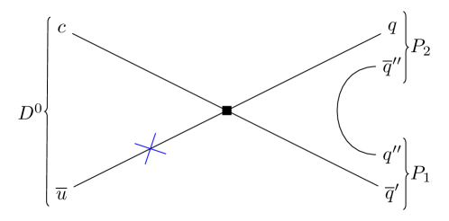
Figure 1: The weak annihilation diagram for $D\rightarrow P_{1}P_{2}\gamma$. The blue cross indicates the dominant photon emission from the light quark of the $D$ meson. Photon emission from the other quark lines is suppressed by powers of $\lambda_{\text{QCD}}/m_{c}$ or $\alpha_{s}$.

We obtain

$$\begin{split}&\mathcal{A}^{\text{WA}}_{-}=i\frac{G_{F}e}{\sqrt{2}}\tilde{C}\frac{f_{D}Q_{u}}{\lambda_{D}(v\cdot k)}\sum_{q,q^{\prime}\in\{d,s\}}V_{cq}^{*}V_{uq^{\prime}}f^{P_{1}P_{2}}_{(q,q^{\prime})}(s)\,,\\ &\mathcal{A}^{\text{WA}}_{+}=\frac{G_{F}e}{\sqrt{2}}\tilde{C}\frac{f_{D}Q_{u}}{\lambda_{D}(v\cdot k)}\sum_{q,q^{\prime}\in\{d,s\}}V_{cq}^{*}V_{uq^{\prime}}f^{P_{1}P_{2}}_{(q,q^{\prime})}(s)\,,\end{split}$$ (10)

where $Q_{u}=2/3$ denotes the electric charge of the up-type quarks, and we decomposed $P=v\,m_{D}$. The nonperturbative parameter $\lambda_{D}\sim\Lambda_{\text{QCD}}$ is poorly known and thus source of large theoretical uncertainties. In the following we use $\lambda_{D}=0.1\,{\rm GeV}$ deBoer:2017que . For the final states $\pi^{+}\pi^{-}\gamma$ and $K^{+}K^{-}\gamma$, the remaining form factors $f^{P_{1}P_{2}}_{(q,q^{\prime})}(s)$ can be expressed in terms of the electromagnetic pion and kaon form factors Bruch:2004py . For the final states $\pi^{+}K^{-}\gamma$ and $\pi^{0}\overline{K}\gamma$, we use the form factors extracted from $\tau^{-}\rightarrow\nu_{\tau}K_{s}\pi^{0}$ decays Boito:2008fq in combination with isospin relations. We obtain for the non-vanishing form factors

$$\begin{split}&f^{\pi^{+}\pi^{-}}_{(d,d)}(s)=-F^{\text{em}}(s)\,,\\ &f^{K^{+}K^{-}}_{(d,d)}(s)=3F^{(I=0)}_{K^{+}}(s)-F^{(I=1)}_{K^{+}}(s)\,,\\ &f^{K^{+}K^{-}}_{(s,s)}(s)=-3F^{s}_{K^{+}}(s)\,,\\ &f^{\pi^{+}K^{-}}_{(s,d)}(s)=-f^{\overline{K}\pi^{-}}_{+}(s)\,,\\ &f^{\pi^{0}\overline{K}^{0}}_{(s,d)}(s)=\frac{1}{\sqrt{2}}f^{\overline{K}\pi^{-}}_{+}(s)\,.\end{split}$$ (11)

More details about the form factors are given in appendix B.1. We recall that QCDF holds for light and energetic $P_{1}$–$P_{2}$ systems. This limits the validity of the results to $s\lesssim 1.5\,{\rm GeV}^{2}$, corresponding to an approximate upper limit on a light hadron’s or hadronic system’s invariant mass squared, including the $\phi$. The WA decay amplitudes are independent of $t$.

II.3 Soft photon approximation

Complementary to QCDF, we use Low’s theorem Low:1958 to estimate the decay amplitudes in the limit of soft photons. This approach holds for photon energies below $m_{P}^{2}/E_{P}$ DelDuca:1990 , which results in $s\gtrsim 2.3\,{\rm GeV}^{2}$ for $D\rightarrow K^{+}K^{-}\gamma$ and $s\gtrsim 3.4\,{\rm GeV}^{2}$ for decays with a final-state pion. The amplitude is then given by Cappiello:2012vg

$$\mathcal{A}_{-}^{\rm Low}=-\frac{e\mathcal{A}(D\to P_{1}P_{2})}{(p_{1}\cdot k)(p_{2}\cdot k)}\,,$$ (12)

while $\mathcal{A}_{+}^{\rm Low}=0$. There is no such contribution to $D\to\pi^{0}\bar{K}^{0}\gamma$, since only neutral mesons are involved. The modulus of the $D\rightarrow P_{1}P_{2}$ amplitudes can be extracted from branching ratio data using

$$\mathcal{B}(D\rightarrow P_{1}P_{2})=\frac{|\mathcal{A}(D\rightarrow P_{1}P_{2})|^{2}}{16\pi m_{D}\Gamma_{D}}\sqrt{\left(1-\frac{(m_{1}+m_{2})^{2}}{m_{D}^{2}}\right)\left(1-\frac{(m_{1}-m_{2})^{2}}{m_{D}^{2}}\right)}\,,$$ (13)

where $\Gamma_{D}$ is the total width of the D meson. Using the parameters given in appendix A, we obtain

$$\begin{split}&\left|\mathcal{A}(D\rightarrow\pi^{+}\pi^{-})\right|=(4.62\pm 0.04)\cdot 10^{-7}\,\text{GeV}\,,\\ &\left|\mathcal{A}(D\rightarrow\pi^{+}K^{-})\right|=(2.519\pm 0.014)\cdot 10^{-6}\,\text{GeV}\,,\\ &\left|\mathcal{A}(D\rightarrow K^{+}K^{-})\right|=(8.38\pm 0.09)\cdot 10^{-7}\,\text{GeV}\,.\end{split}$$ (14)

Low’s theorem predicts that the differential decay rate behaves as DAmbrosio:1994bks

$$\frac{d{}\Gamma}{d{}s}\sim\frac{1}{m_{D}^{2}-s}\,.$$ (15)

Consequently, there is a singularity at the boundary of the phase space. This corresponds to a vanishing photon energy in the $D$ meson’s rest frame. The tail of the singularity dominates the decay rate for small photon energies. We remove these events for integrated rates by cuts in the photon energy, as they are of known SM origin and hamper access to flavor and BSM dynamics.

II.4 HH$\chi$PT

As a third theory description we use the framework of heavy hadron chiral perturbation theory (HH$\chi$PT), which contains both the heavy quark and the $SU(3)_{L}\times SU(3)_{R}$ chiral symmetry. The effective Lagrangian was introduced in Wise:1992 ; Burdman:1992 ; Yan:1992 and extended by light vector resonances by Casalbuoni et al. Casalbuoni:1993 . We follow the approach of Fajfer et al., who studied radiative two-body decays $D\rightarrow V\gamma$ Bajc:1994ui ; Fajfer:1998dv and Cabibbo allowed three-body decays $D\rightarrow K^{-}\pi^{+}\gamma$ Fajfer:2002bq and $D\rightarrow\overline{K}^{0}\pi^{0}\gamma$ Fajfer:2002xf in this way.
The light mesons are described by $3\times 3$ matrices

$$u=\exp\left(\frac{\mathrm{i}\Pi}{f}\right)\,,\qquad\Pi=\left(\begin{array}[]{ccc}\frac{\pi^{0}}{\sqrt{2}}+\frac{\eta_{8}}{\sqrt{6}}&\pi^{+}&K^{+}\\ \pi^{-}&-\frac{\pi^{0}}{\sqrt{2}}+\frac{\eta_{8}}{\sqrt{6}}&K^{0}\\ K^{-}&\overline{K}^{0}&-\frac{2\eta_{8}}{\sqrt{6}}\\ \end{array}\right)\,,$$ (19)

$$\hat{\rho}_{\mu}=\mathrm{i}\frac{g_{v}}{\sqrt{2}}\rho_{\mu}\,,\qquad\rho_{\mu}=\left(\begin{array}[]{ccc}\frac{\rho_{\mu}^{0}+\omega_{\mu}}{\sqrt{2}}&\rho_{\mu}^{+}&K^{\star+}_{\mu}\\ \rho_{\mu}^{-}&\frac{-\rho_{\mu}^{0}+\omega_{\mu}}{\sqrt{2}}&K^{\star 0}_{\mu}\\ K^{\star-}_{\mu}&\overline{K}^{\star 0}_{\mu}&\Phi_{\mu}\\ \end{array}\right)\,,$$ (23)

where $f\simeq f_{\pi}$ is the pion decay constant and $g_{v}=5.9$ Bando:1985 . To write down the photon interaction with the light mesons in a simple way, we define two currents

$$\begin{split}\mathcal{V}_{\mu}&=\frac{1}{2}\left(u^{\dagger}D_{\mu}u+uD_{\mu}u^{\dagger}\right)\,,\\ \mathcal{A}_{\mu}&=\frac{1}{2}\left(u^{\dagger}D_{\mu}u-uD_{\mu}u^{\dagger}\right)\,.\end{split}$$ (24)

Here, the covariant derivative acting on $u$ and $u^{\dagger}$ is given by $D_{\mu}u^{(\dagger)}=\partial_{\mu}u^{(\dagger)}+\mathrm{i}eB_{\mu}Qu^{(\dagger)}$, with the photon field $B_{\mu}$ and the diagonal charge matrix $Q=\text{diag}(2/3,-1/3,-1/3)$. The even-parity strong Lagrangian for light mesons is then given by Bando:1985

$$\mathcal{L}_{\text{light}}=-\frac{f^{2}}{2}\left[\operatorname{Tr}_{F}\left(\mathcal{A}_{\mu}\mathcal{A}^{\mu}\right)+a\operatorname{Tr}_{F}\left(\left(\mathcal{V}_{\mu}-\hat{\rho}_{\mu}\right)^{2}\right)\right]+\frac{1}{2g_{v}^{2}}\operatorname{Tr}_{F}\left(F_{\mu\nu}(\hat{\rho})F^{\mu\nu}(\hat{\rho})\right)\,,$$ (25)

where $F_{\mu\nu}(\hat{\rho})=\partial_{\mu}\hat{\rho}_{\nu}-\partial_{\nu}\hat{\rho}_{\mu}+\left[\hat{\rho}_{\mu},\hat{\rho}_{\nu}\right]$ denotes the field strength tensor of the vector resonances. In general, $a$ is a free parameter, which satisfies $a=2$ in case of exact vector meson dominance (VMD). In VMD there is no direct vertex that connects two pseudoscalars and a photon. In this case, the photon couples to pseudoscalars via a virtual vector meson. Analogously, the matrix element $\braket{P_{1}P_{2}}{\overline{q}\gamma^{\mu}(1-\gamma_{5})q^{\prime}}{0}$ also vanishes. However, we do not use the case of VMD and exact flavor symmetry, but allow for $SU(3)$ breaking effects. Therefore, we choose to set $a=1$ and replace the model coupling $g_{v}$, decay constant $f$, and vector meson mass $m_{V}=\sqrt{a/2}g_{v}f$ in $\mathcal{L}_{\text{light}}$ with the respective measured masses, decay constants and couplings $g_{v}=\sqrt{2}m_{V}^{2}/g_{V}$. They are defined by

$$\braket{V(q,\eta)}{j_{V}^{\mu}}{0}=\eta^{*\mu}(q)g_{V}(q^{2})\,,$$ (26)

where $j_{K^{\star},\overline{K}^{\star},K^{\star\pm},\Phi}^{\mu}=\overline{q}\gamma^{\mu}q^{\prime}$ and $j_{\omega,\rho}^{\mu}=\frac{1}{\sqrt{2}}(\overline{u}\gamma^{\mu}u\pm\overline{d}\gamma^{\mu}d)$. Here, $q$ and $\eta$ denote the vector meson’s momentum and polarization vector, respectively. For our numerical evaluation we use $g_{V}(0)\simeq g_{V}(m_{V}^{2})=m_{V}f_{V}$, where $f_{V}$ is the vector meson decay constant with mass dimension one. With these couplings the following $V\gamma$ interactions arise Fajfer:1998dv

$$\mathcal{L}_{V_{0}\gamma}=-\frac{e}{\sqrt{2}}B_{\mu}\left(g_{\rho}\rho^{0\mu}+\frac{1}{3}g_{\omega}\omega^{\mu}-\frac{\sqrt{2}}{3}g_{\Phi}\Phi^{\mu}\right)\,.$$ (27)

Instead of the VVP interactions generated by the odd-parity Lagrangian Bramon:1995 , we use effective VP$\gamma$ interactions

$$\mathcal{L}_{VP\gamma}=-\frac{1}{2}eg_{VP\gamma}\epsilon_{\mu\nu\rho\sigma}F^{\mu\nu}(B)\partial^{\rho}V^{\sigma}P^{\dagger}+\text{h.c.}$$ (28)

and determine the effective coefficients $g_{VP\gamma}$ from experimental data Fajfer:2002bq ; Fajfer:1997bh

$$\Gamma(V\rightarrow P\gamma)=\frac{\alpha_{\text{em}}m_{V}^{3}}{24}|g_{VP\gamma}|^{2}\left(1-\frac{m_{P}^{2}}{m_{V}^{2}}\right)^{3}\,.$$ (29)

The heavy pseudoscalar and vector mesons are represented by $4\times 4$ matrices

$$\begin{split}H_{a}&=\frac{1}{2}\left(1+\not{v}\right)\left(P^{\star}_{a\mu}\gamma^{\mu}-P_{a}\gamma_{5}\right)\,,\\ \overline{H}_{a}&=\gamma^{0}H_{a}^{\dagger}\gamma^{0}=\left(P^{\star\dagger}_{a\mu}\gamma^{\mu}+P^{\dagger}_{a}\gamma_{5}\right)\frac{1}{2}\left(1+\not{v}\right)\,,\end{split}$$ (30)

where $P^{\star(\dagger)}_{a\mu}$, $P^{(\dagger)}_{a}$ annihilate (create) a heavy spin-one and spin-zero meson $h_{a}$ with quark flavor content $c{\overline{q}_{a}}$ and velocity $v$, respectively. The annihilation operators are normalized as

$$\begin{split}&\braket{0}{P_{a}}{h_{a}(v)}=1\,,\\ &\braket{0}{P_{a}^{\star\mu}}{h_{a}^{\star}(v,\eta)}=\eta^{\mu}\,.\end{split}$$ (31)

The heavy-meson Lagrangian reads

$$\begin{split}\mathcal{L}_{\text{heavy}}&=\mathrm{i}\operatorname{Tr}_{D}\left(H_{a}v_{\mu}\left(D^{\mu}\right)_{ab}\overline{H}_{b}\right)+\mathrm{i}g\operatorname{Tr}_{D}\left(H_{a}\gamma_{\mu}\gamma_{5}(\mathcal{A}^{\mu})_{ab}\overline{H}_{b}\right)\\ &\quad+\mathrm{i}\tilde{\beta}\operatorname{Tr}_{D}\left(H_{a}v_{\mu}\left(\mathcal{V}^{\mu}-\hat{\rho}^{\mu}\right)_{ab}\overline{H}_{b}\right)\,,\end{split}$$ (32)

where the covariant derivative is defined as $\left(D^{\mu}\right)_{ab}\overline{H}_{b}=\partial^{\mu}\overline{H}_{a}+\left(\mathcal{V}^{\mu}\right)_{ab}\overline{H}_{b}-\mathrm{i}eQ_{c}B^{\mu}\overline{H}_{a}$, with the electric charge of the charm quark $Q_{c}=2/3$. The parameter $g=0.59$ was determined by experimental data of strong $D^{\star}\rightarrow D\pi$ decays Singer:1999ak ; Anastassov:2001cw . The coupling $\tilde{\beta}$ seems to be very small and will be neglected Bajc:1997ey . The odd-parity Lagrangian for the heavy mesons is given by

$$\mathcal{L}=\mathrm{i}\lambda\operatorname{Tr}\left(H_{a}\sigma_{\mu\nu}F^{\mu\nu}(\hat{\rho})_{ab}\overline{H}_{b}\right)-\lambda^{\prime}e\operatorname{Tr}\left(H_{a}\sigma_{\mu\nu}F^{\mu\nu}(B)\overline{H}_{a}\right)\,,$$ (33)

with $\sigma_{\mu\nu}=\frac{\mathrm{i}}{2}\left[\gamma_{\mu},\gamma_{\nu}\right]$. The couplings $\lambda$ and $\lambda^{\prime}$ can be extracted from rations $R_{\gamma}^{0/+}=\Gamma(D^{\star 0/+}\rightarrow D^{0/+}\gamma)/\Gamma(D^{\star 0/+}\rightarrow D^{0/+}\pi)$. $\lambda=-0.49\,{\rm GeV}^{-1}$ and $\lambda^{\prime}=-0.102\,{\rm GeV}^{-1}$ are in good agreement with data Fajfer:2002bq . The partonic weak currents can be expressed in terms of chiral currents as Bajc:1995km ; Bajc:1994ui

$$\begin{split}(\overline{q}_{a}Q)^{\mu}_{\text{V-A}}\simeq J_{Q\overline{q}_{a}}^{\mu}&=\frac{1}{2}\mathrm{i}\alpha\operatorname{Tr}\left(\gamma^{\mu}(1-\gamma_{5})H_{b}u_{ba}^{\dagger}\right)+\alpha_{1}\operatorname{Tr}\left(\gamma_{5}H_{b}\left(\hat{\rho}^{\mu}-\mathcal{V}^{\mu}\right)_{bc}u_{ca}^{\dagger}\right)\\ &+\alpha_{2}\operatorname{Tr}\left(\gamma^{\mu}\gamma_{5}H_{b}v_{\alpha}(\hat{\rho}^{\alpha}-\mathcal{V}^{\alpha})_{bc}u_{ca}^{\dagger}\right)+\ldots\,,\\ (\overline{q}_{j}q_{i})_{\text{V-A}}^{\mu}\simeq J_{ij}^{\mu}&=\mathrm{i}f^{2}\left\{u\left[\mathcal{A}^{\mu}+a\left(\mathcal{V}^{\mu}-\hat{\rho}^{\mu}\right)\right]u^{\dagger}\right\}_{ij}\,,\end{split}$$ (34)

where the ellipsis denotes higher-order terms in the chiral and heavy-quark expansions. The definition of the heavy-meson decay constants implies $\alpha=f_{h}\sqrt{m_{h}}$. The parameters $\alpha_{1}$ and $\alpha_{2}$ can be extracted from $D\rightarrow V$ transition form factors Fajfer:2002bq

$$\begin{split}A_{1}(q^{2}_{\text{max}})=2\frac{\sqrt{m_{D}}}{m_{D}+m_{V}}\frac{m_{V}^{2}}{g_{V}}\alpha_{1}\,,\qquad A_{2}(q^{2}_{\text{max}})=2\frac{m_{D}+m_{V}}{m_{D}^{\frac{3}{2}}}\frac{m_{V}^{2}}{g_{V}}\alpha_{2}\,.\end{split}$$ (35)

Using the $D\to K^{\star}$ form factors Verma:2011yw we obtain $\alpha_{1}=0.188\,{\rm GeV}^{\frac{1}{2}}$ and $\alpha_{2}=0.086\,{\rm GeV}^{\frac{1}{2}}$. The signs in (35) are due to the conventions in Verma:2011yw . The weak tensor current is given by Casalbuoni:1993nh

$$\begin{split}&\overline{q}\sigma^{\mu\nu}(1+\gamma_{5})Q\simeq J_{Q\overline{q}_{a}}^{\mu\nu}\\ &=\frac{1}{2}\mathrm{i}\alpha\operatorname{Tr}\left(\sigma^{\mu\nu}(1+\gamma_{5})H_{b}u_{ba}^{\dagger}\right)\\ &\quad+\mathrm{i}\alpha_{1}\left(g^{\mu\alpha}g^{\nu\beta}-\frac{1}{2}i\epsilon^{\mu\nu\alpha\beta}\right)\operatorname{Tr}\left(\gamma_{5}H_{b}\left[\gamma_{\alpha}\left(\hat{\rho}_{\beta}-\mathcal{V}_{\beta}\right)_{bc}-\gamma_{\beta}\left(\hat{\rho}_{\alpha}-\mathcal{V}_{\alpha}\right)_{bc}\right]u_{ca}^{\dagger}\right)\\ &\quad-\alpha_{2}\operatorname{Tr}\left(\sigma^{\mu\nu}\gamma_{5}H_{b}v_{\alpha}\left(\hat{\rho}^{\alpha}-\mathcal{V}^{\alpha}\right)_{bc}u^{\dagger}_{ca}\right)+\ldots\,,\end{split}$$ (36)

where, again, the ellipsis denotes higher-order terms in the chiral and heavy-quark expansions.

The parity-even and parity-odd amplitudes are given in terms of four form factors

$$\begin{split}&A_{-}^{\rm HH\chi PT}=\frac{G_{F}e}{\sqrt{2}}\sum_{q,q^{\prime}\in\{d,s\}}V_{cq}^{*}V_{uq^{\prime}}\left[(C_{2}-\frac{1}{6}C_{1})\sum_{i}A_{i}^{(q,q^{\prime})}+\frac{1}{2}C_{1}\sum_{i}E_{i}^{(q,q^{\prime})}\right]\,,\\ &A_{+}^{\rm HH\chi PT}=\frac{G_{F}e}{\sqrt{2}}\sum_{q,q^{\prime}\in\{d,s\}}V_{cq}^{*}V_{uq^{\prime}}\left[(C_{2}-\frac{1}{6}C_{1})\sum_{i}B_{i}^{(q,q^{\prime})}+\frac{1}{2}C_{1}\sum_{i}D_{i}^{(q,q^{\prime})}\right]\,.\end{split}$$ (37)

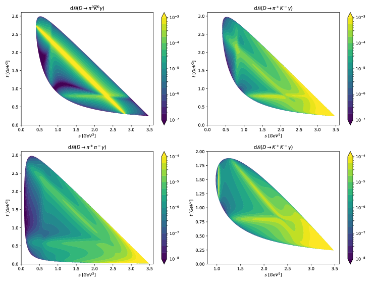
Figure 2: SM Dalitz plots for the decays $D\to\overline{K}^{0}\pi^{0}\gamma$ (upper left), $D\to K^{-}\pi^{+}\gamma$ (upper right), $D\to\pi^{+}\pi^{-}\gamma$ (lower left) and $D\to K^{+}K^{-}\gamma$ (lower right) based on HH$\chi$PT at $\mu_{c}=m_{c}$.

Here, $A$ and $B$ belong to the charged current operator $(\overline{u}q^{\prime})_{\mu V-A}(\overline{q}c)^{\mu}_{V-A}\equiv 4O_{2}^{(q^{\prime},q)}$ and D and E to the neutral current operator $(\overline{q}q^{\prime})_{\mu V-A}(\overline{u}c)^{\mu}_{V-A}\equiv 8O_{1}^{(q^{\prime},q)}+4O_{2}^{(q^{\prime},q)}/3$. The corresponding diagrams are shown in Fig. 18 and 19. The non-zero contributions are listed in Appendix B.2, where we also provide a list with differences between our results and those in Ref. Fajfer:2002bq . We neglect the masses of the light mesons in the form factors, but consider them in the phase space. To enforce Low’s theorem, we remove the bremsstrahlung contributions $A_{1,2}$ in (37) and add (12) to $A_{-}^{\rm HH\chi PT}$. For the strong phase we have taken the value predicted by HH$\chi$PT. In Fig. 2 we show Dalitz plots based on the SM HH$\chi$PT predictions. Besides the dominant bremsstrahlung effects for large s, the intermediate $\rho$, $\omega$, $K^{\star}$ and $\Phi$ resonances are clearly visible as bands in $s,t$ and the third Mandelstam variable, $u=(p_{1}+k)^{2}=m_{D}^{2}+m_{1}^{2}+m_{2}^{2}-s-t$.

III Comparison of QCD frameworks

In this section, we compare the predictions obtained using the different QCD methods in Section II. We anticipate quantitative and qualitative differences between QCDF to leading order and HH$\chi$PT. First, we study differential and integrated branching ratios in Section III.1. In Section III.2 we propose to utilze a forward-backward asymmetry, defined below in Eq. (38), to help disentangling the resonance contributions to the branching ratios. This subsequently improves the NP sensitivity of the $D\to P^{+}P^{-}\gamma$ decays. We consider the U-spin link, exploited already for polarization-asymmetries in radiative charm decays deBoer:2018zhz , in Section III.3.

III.1 Branching ratios

The branching ratios for the various decay modes, obtained from QCDF (blue bands), HH$\chi$PT (green bands) and Low’s theorem (red dashed lines), are shown in Fig. 3. The width of the bands represents the theoretical uncertainty due to the $\mu_{c}$ dependence of the Wilson coefficients.

The shape of the QCDF results is mainly given by the $P_{1}-P_{2}$ form factors and their resonance structure. For the $D\to P_{1}^{+}P_{2}^{-}\gamma$ decays, the high-$s$ regions of the HH$\chi$PT predictions are dominated by bremsstrahlung effects. Since we have replaced the model’s own bremsstrahlung contributions by those of Low’s theorem, the results approach each other asymptotically towards the large-$s$ endpoint. Without this substitution, the differential branching ratios from HH$\chi$PT in this region would be about one order of magnitude larger. For lower $s$, the impact of the resonances becomes visible.

In the soft photon approximation the photon couples directly to the mesons. Therefore, there is no such contribution for the $D\to\pi^{0}\overline{K}^{0}\gamma$ decay. Its distribution is dominated by the $\omega$ resonance which has a significant branching ratio to $\pi^{0}\gamma$; this is manifest in the Dalitz plot in Fig. 2.

Apart from the $K^{*},\rho$, and $\phi$ peaks, the shapes of the differential branching ratios differ significantly between QCDF and HH$\chi$PT, due to the $t$ and $u$-channel resonance contributions in the latter. This is shown in the Dalitz plot in Fig. 2.

In Table 1 we give the SM branching ratios for the four decay modes. We employ phase space cuts $s\leq 1.5\leavevmode\nobreak\ {\rm GeV}^{2}$, the region of applicability of QCDF, or $E_{\gamma}\geq 0.1\leavevmode\nobreak\ {\rm GeV}$, corresponding to $s\leq 3.1\leavevmode\nobreak\ {\rm GeV}^{2}$, to avoid the soft photon pole. Here, $E_{\gamma}=(m_{D}^{2}-s)/(2m_{D})$ is the photon energy in the $D$ meson’s rest frame. Applying the same cuts in both cases, the HH$\chi$PT branching ratios are generally larger than the QCDF ones, except for the $D\to K^{+}K^{-}\gamma$ mode, where they are of comparable size.

We recall that SM branching ratios within leading order QCDF are proportional to $(1/\lambda_{D})^{2}$. Since $\lambda_{D}$ is of the order of $\Lambda_{\rm QCD}$ and we employ a rather low value $\lambda_{D}=0.1\,{\rm GeV}$ deBoer:2017que , the values in Table 1 should be regarded as maximal branching ratios. The large uncertainty of these values arises from the residual scale dependence of the Wilson coefficient $\bar{C}$ (9). A measurement of the branching ratios of the SM-like modes $D\to K\pi\gamma$ thus provides an experimentally extracted value of $\bar{C}/\lambda_{D}$. Color-allowed modes feature Wilson coefficients with significantly smaller scale uncertainty, and allow for a cleaner, direct probe of $\lambda_{D}$ deBoer:2017que . While $\lambda_{D}$ is poorly known, it effectively drives the annihilation with initial state radiation and experimental constraints are informative even in the presence of sizable systematic uncertainties inherent to QCDF in charm.

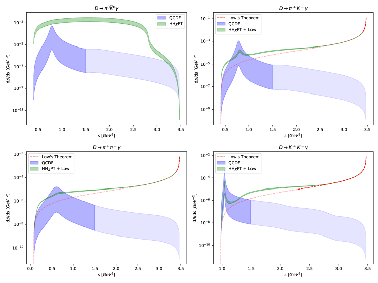
Figure 3: The SM predictions for the differential branching ratios of the decays $D\to\overline{K}^{0}\pi^{0}\gamma$ (upper left), $D\to K^{-}\pi^{+}\gamma$ (upper right), $D\to\pi^{+}\pi^{-}\gamma$ (lower left) and $D\to K^{+}K^{-}\gamma$ (lower right). Blue bands correspond to QCDF, green bands to HH$\chi$PT and the red dashed lines to the soft photon approximation. The lighter shaded areas and lines illustrate extrapolations beyond the model’s region of applicability. QCDF branching ratios are obtained for $\lambda_{D}=0.1\,{\rm GeV}$ and are $\propto(0.1\,{\rm GeV}/\lambda_{D})^{2}$.

	$D\to\pi^{0}\overline{K}^{0}\gamma$	$D\to\pi^{+}K^{-}\gamma$	$D\to\pi^{+}\pi^{-}\gamma$	$D\to K^{+}K^{-}\gamma$
$\text{QCDF}\big{|}^{\text{SM}}_{s\leq 1.5\leavevmode\nobreak\ {\rm GeV}^{2}}$	$(0.04-6.36)\cdot 10^{-5}$	$(0.01-1.28)\cdot 10^{-4}$	$(0.04-5.16)\cdot 10^{-6}$	$(0.05-9.92)\cdot 10^{-6}$
$\text{HH$\chi$PT}\big{|}^{\text{SM}}_{s\leq 1.5\leavevmode\nobreak\ {\rm GeV}^{2}}$	$(0.9-2.2)\cdot 10^{-3}$	$(7.2-9.2)\cdot 10^{-5}$	$(6.2-7.1)\cdot 10^{-6}$	$(1.1-1.6)\cdot 10^{-6}$
$\text{HH$\chi$PT}\big{|}^{\text{SM}}_{E_{\gamma}\geq 0.1\leavevmode\nobreak\ {\rm GeV}}$	$(2.1-5.0)\cdot 10^{-3}$	$(6.7-7.2)\cdot 10^{-4}$	$(3.9-4.1)\cdot 10^{-5}$	$(3.2-3.5)\cdot 10^{-5}$
$\text{QCDF}\big{|}^{\text{BSM}}_{s\leq 1.5\leavevmode\nobreak\ {\rm GeV}^{2}}$	-	-	$(0.6-1.7)\cdot 10^{-5}$	$(0.1-10.5)\cdot 10^{-6}$
$\text{HH$\chi$PT}\big{|}^{\text{BSM}}_{s\leq 1.5\leavevmode\nobreak\ {\rm GeV}^{2}}$	-	-	$(0.9-1.7)\cdot 10^{-5}$	$(0.9-1.7)\cdot 10^{-6}$
$\text{HH$\chi$PT}\big{|}^{\text{BSM}}_{E_{\gamma}\geq 0.1\leavevmode\nobreak\ {\rm GeV}}$	-	-	$(4.3-5.3)\cdot 10^{-5}$	$(3.2-3.6)\cdot 10^{-5}$

Table 1: SM and BSM branching ratios for $D\to\pi^{0}\overline{K}^{0}\gamma$ , $D\to\pi^{+}K^{-}\gamma$, $D\to\pi^{+}\pi^{-}\gamma$ and $D\to K^{+}K^{-}\gamma$. QCDF is applicable for $s\lesssim 1.5\,{\rm GeV}^{2}$; to enable sensible comparison we also provide HH$\chi$PT branching ratios with this cut. Also given are HH$\chi$PT predictions for $E_{\gamma}\geq 0.1\,{\rm GeV}$, see text for details. The QCDF branching ratios are obtained for $\lambda_{D}=0.1\,{\rm GeV}$. The SM predictions are $\propto(0.1\,{\rm GeV}/\lambda_{D})^{2}$.

III.2 Forward-Backward Asymmetry

Angular observables are also suitable for testing QCD models. We define the forward-backward asymmetry

$$\begin{split}&A_{\rm FB}(s)=\frac{\int_{t_{\rm min}}^{t_{\rm 0}}dt\frac{d{}^{2}\Gamma}{d{}sd{}t}-\int_{t_{\rm 0}}^{t_{\rm max}}dt\frac{d{}^{2}\Gamma}{d{}sd{}t}}{\int_{t_{\rm min}}^{t_{\rm 0}}dt\frac{d{}^{2}\Gamma}{d{}sd{}t}+\int_{t_{\rm 0}}^{t_{\rm max}}dt\frac{d{}^{2}\Gamma}{d{}sd{}t}}\,,\\ &t_{\rm 0}=\frac{1}{2s}\left(-s^{2}+s(m_{D}^{2}+m_{1}^{2}+m_{2}^{2})+m_{D}^{2}(m_{2}^{2}-m_{1}^{2})\right)\,,\end{split}$$ (38)

where the first (second) term in the numerator corresponds to $0\leq\cos(\theta_{2\gamma})\leq 1$ $(-1\leq\cos(\theta_{2\gamma})\leq 0)$. Here, $\theta_{2\gamma}$ is the angle between $P_{2}$ and the photon in the $P_{1}-P_{2}$ center-of-mass frame. In Fig. 4 we show the SM forward-backward asymmetry based on HH$\chi$PT. In all decay modes $A_{\rm FB}(s)$ is dominated by intermediate vector resonances. To illustrate this, the forward-backward asymmetries are also shown without or only with individual resonance contributions. The $(P_{1}P_{2})_{\text{res}}$ resonances contribute to $A_{\rm FB}$ only via interference terms, since the corresponding form factors depend only on $s$. For $D\to\pi^{+}\pi^{-}\gamma$ and $D\to K^{+}K^{-}\gamma$ the diagrams of the neutral current operator, which contain $(P_{1}\gamma)_{\text{res}}$ and $(P_{2}\gamma)_{\text{res}}$ resonances, give the same contribution to the amplitude in the forward and backward region of the phase space. For $P_{1}\neq\overline{P}_{2}$ this symmetry does not exist. In case of the charged current operator, these resonances contribute in different ways to the forward and backward region due to the asymmetric factorization of the diagrams $B_{3}$ (69), (72), (75). This effect is primarily responsible for the shape of $A_{\rm FB}$ in $D\to\pi^{+}\pi^{-}\gamma$ and $D\to K^{+}K^{-}\gamma$ decays. $A_{\rm FB}(D\to\pi^{0}\overline{K}^{0}\gamma)$ is, like the differential branching ratio shown in Fig. 2, dominated by the $\omega$ resonance.

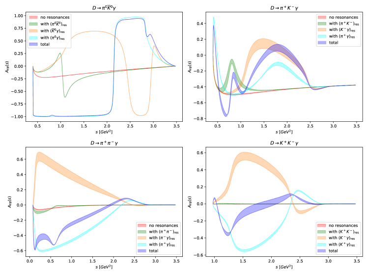
Figure 4: The forward-backward asymmetry $A_{\rm FB}(s)$ (38) as a function of $s$. The red bands contain only non-resonant contributions. The green, orange and light blue bands contain additional contributions of a specific resonance channel. The dark blue bands are the complete forward-backward asymmetries according to HH$\chi$PT. To leading order QCDF $A_{\rm FB}(s)=0$.

Since the WA form factors are only dependent on $s$, the SM forward-backward asymmetry vanishes to leading order QCDF. Therefore, we add contributions from $t$ and $u$-channel resonances using a phenomenological approach. To this end, we combine $D\to VP$ amplitudes with the effective $VP\gamma$ coupling from equation (28).

Figure 5: The dominant diagrams to $D\to VP(\to PP\gamma)$ in the $\lambda_{\text{QCD}}/m_{c}$ and $\alpha_{s}$ expansion. At order $\alpha_{s}^{0}$ QCDF reproduces the naive factorization Beneke:2000ry . The diagrams are shown for charged final state mesons. For the final state with uncharged mesons the $u$ and $q$ quark have to be exchanged.

We obtain

$$\begin{split}\mathcal{A}^{\text{pheno}}_{+}=\frac{G_{F}e}{\sqrt{2}}V_{cq}^{*}V_{uq^{\prime}}\left(C_{2}-\frac{1}{6}C_{1}\right)\left(\frac{2m_{V}f_{P}g_{VP\gamma}A_{0}^{DV}(m_{1}^{2})}{(p_{2}+k)^{2}-m_{V}^{2}+\mathrm{i}m_{V}\Gamma_{V}}+\frac{2m_{V}f_{V}g_{VP\gamma}F_{1}^{DP}((p_{1}+k)^{2})}{(p_{1}+k)^{2}-m_{V}^{2}+\mathrm{i}m_{V}\Gamma_{V}}\right)\,,\end{split}$$ (39)

where the first (second) term in (39) corresponds to the left (right) diagram in Fig. 5. The amplitude for the final state $\pi^{0}\overline{K}^{0}\gamma$ can be obtained from Eq (39) by substituting $C_{2}-1/6C_{1}\rightarrow C_{2}/2$, $m_{1}\to m_{2}$, and $p_{1}\leftrightarrow p_{2}$, and multiplying by the factor $-1/\sqrt{2}$. The $D\to P$ and $D\to V$ transition form factors are taken from Ref. Verma:2011yw . As expected, resulting distributions based on (39) exhibit the same main resonance features as the ones in HHchiPT, and are therefore not shown.

III.3 The U-spin link

We further investigate the U-spin link between the SM-dominated mode $D\to K^{-}\pi^{+}\gamma$ and the BSM-probes $D\to\pi^{+}\pi^{-}\gamma$ and $D\to K^{+}K^{-}\gamma$. In practise, a measurement of ${\cal{B}}(D\to K^{-}\pi^{+}\gamma)$ can provide a data-driven SM prediction for the branching ratios of the FCNC decays. The method is phenomenological and serves, in the case of branching ratios, as an order-of-magnitude estimate. The U-spin approximation is expected to yield better results in ratios of observables (which arise already at lowest order in the U-spin limit), such that overall systematics drops out. Useful applications have been made for polarization asymmetries in $D\to V\gamma$ decays deBoer:2018zhz . However, three-body radiative decays are considerably more complicated due to the intermediate resonances, and we do not pursue the U-spin link for the forward-backward or CP asymmetries.

A comparison between $|V_{us}|^{2}/|V_{ud}|^{2}d{\cal{B}}(D\to K^{-}\pi^{+}\gamma)/ds$ with $d{\cal{B}}(D\to K^{+}K^{-}\gamma)/ds$ and $|V_{cd}|^{2}/|V_{cs}|^{2}d{\cal{B}}(D\to K^{-}\pi^{+}\gamma)/ds$ with $d{\cal{B}}(D\to\pi^{+}\pi^{-}\gamma)/ds$ is shown in Fig. 6. For $s\gtrsim 1.5\leavevmode\nobreak\ {\rm GeV}$ the predictions of the direct calculations and the U-spin relations are in good agreement. This holds for both the extrapolations of QCDF and the HH$\chi$PT predictions. In the second case this is due to the dominance of the bremsstrahlung contributions and the U-spin relations of the $D\to P_{1}P_{2}$ amplitudes. For $s\lesssim 1.5\leavevmode\nobreak\ {\rm GeV}$, there are large deviations due to the differences in phase space boundaries and the different intermediate resonances.

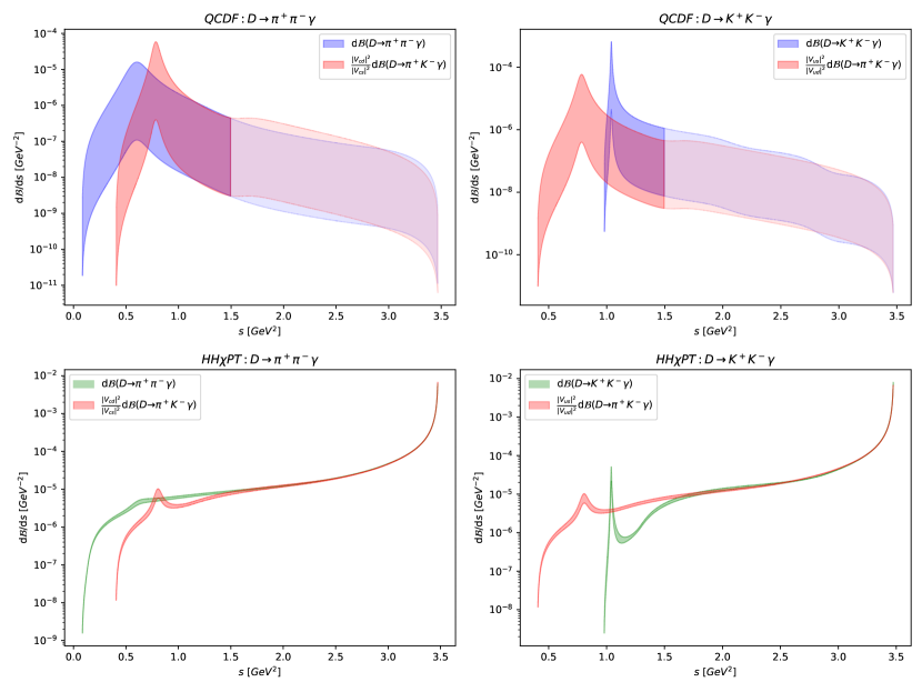
Figure 6: The SM predictions for the differential branching ratios of the decays $D\to\pi^{+}\pi^{-}\gamma$ (left) and $D\to K^{+}K^{-}\gamma$ (right) from a direct QCDF computation (blue bands in upper plots), HH$\chi$PT computations (green bands in lower plots) and from the $D\to K^{-}\pi^{+}\gamma$ distribution multiplied by $|V_{cd}/V_{cs}|^{2}$ and $|V_{us}/V_{ud}|^{2}$, respectively (red bands). The prediction for the SM-like mode $D\to K^{-}\pi^{+}\gamma$ in this figure is from the respective models but could be taken from data.

At the level of integrated SM branching ratios we find

$$\frac{{\cal{B}}-{\cal{B}}(\text{U-spin link})}{{\cal{B}}}\big{|}^{\text{QCDF}}_{s\leq 1.5\leavevmode\nobreak\ {\rm GeV}^{2}}\sim-0.33\,(0.3)\,,$$ (40)

$$\frac{{\cal{B}}-{\cal{B}}(\text{U-spin link})}{{\cal{B}}}\big{|}^{\text{HH$\chi$PT}}_{s\leq 1.5\leavevmode\nobreak\ {\rm GeV}^{2}}\sim 0.35\,(-2.3)\,,$$ (41)

$$\frac{{\cal{B}}-{\cal{B}}(\text{U-spin link})}{{\cal{B}}}\big{|}^{\text{HH$\chi$PT}}_{E_{\gamma}\geq 0.1\leavevmode\nobreak\ {\rm GeV}}\sim 0.07\,(-0.11)\,,$$ (42)

for the $D\to\pi^{+}\pi^{-}(K^{+}K^{-})\gamma$ modes. Eqs. (40)-(42) underline the main features of Fig 6: as a result of the dominance of bremsstrahlung photons from Low’s theorem the corrections (42) are small; the proximity of the $\phi$ to the phase space boundary in $D\to KK\gamma$ makes the U-spin limit in (41) poor. In the other cases the U-spin symmetry performs as expected, within $\sim 30$%.

IV BSM analysis

BSM physics can significantly increase the Wilson coefficients contributing to $c\to u\gamma$ transitions. Examples are supersymmetric models with flavor mixing and chirally enhanced gluino loops, or leptoquarks, see Ref. deBoer:2017que for details. In the following we work out BSM spectra and phenomenology in a model-independent way. Experimental data obtained from $D\rightarrow\rho^{0}\gamma$ decays provide model-independent constraints deBoer:2018buv ; Abdesselam:2016yvr

$$|C_{7}|,|C_{7}^{\prime}|\lesssim 0.3\,.$$ (43)

These values are in agreement with recent studies of $D\to\pi ll$ decays Bause:2019vpr . In Section V.1 we discuss the implications of CP asymmetries in hadronic charm decays that can lead to constraints on the imaginary parts of the dipole operators.

The $D\to P_{1}P_{2}$ matrix elements of the tensor currents can be parameterized as

$$\braket{P_{1}(p_{1})P_{2}(p_{2})}{\overline{u}\sigma^{\mu\nu}k_{\mu}(1\pm\gamma_{5})c}{D(P)}=m_{D}\left[a^{\prime}p_{1}^{\nu}+b^{\prime}p_{2}^{\nu}+c^{\prime}P^{\mu}\mp 2ih^{\prime}\epsilon^{\nu\alpha\beta\gamma}p_{1\alpha}p_{2\beta}k_{\gamma}\right]\,.$$ (44)

with the form factors $a^{\prime},b^{\prime},c^{\prime},h^{\prime}$ given in App. B.2. The form factors depend on $s$ and $t$ and satisfy

$$a^{\prime}p_{1}\cdot k+b^{\prime}p_{2}\cdot k+c^{\prime}P\cdot k=0\,.$$ (45)

The BSM amplitudes are then obtained as

$$\begin{split}&\mathcal{A}_{-}^{\rm BSM}=i\frac{G_{F}e}{\sqrt{2}}\frac{m_{c}}{4\pi^{2}}(C_{7}+C_{7}^{\prime})\frac{(b^{\prime}-a^{\prime})}{v\cdot k}\,,\\ &\mathcal{A}_{+}^{\rm BSM}=\frac{G_{F}e}{\sqrt{2}}\frac{m_{c}m_{D}}{2\pi^{2}}(C_{7}-C_{7}^{\prime})h^{\prime}\,.\end{split}$$ (46)

In Figs. 7 and 8 we show differential branching ratios for the FCNC modes based on QCDF and HH$\chi$PT, respectively, both in the SM (blue) and in different BSM scenarios. One of the BSM coefficients, $C_{7}$ or $C_{7}^{\prime}$, is set to zero while the other one is taken to saturate the limit (43) with CP-phases $0,\pm\pi/2,\pi$. The same conclusions are drawn for both QCD approaches: the $D\to K^{+}K^{-}\gamma$ branching ratio is insensitive to NP in the dipole operators. In particular, the benchmarks for $O_{7}^{\prime}$ and the SM prediction are almost identical. For $O_{7}$ small deviations occur directly beyond the $\phi$ peak. On the other hand, BSM contributions can increase the differential branching ratio of $D\to\pi^{+}\pi^{-}\gamma$ by up to one order of magnitude around the $\rho$ peak. However, due to the intrinsic uncertainties from the Breit-Wigner contributions around the resonance peaks it is difficult to actually claim sensitivity to NP. This is frequently the case in $D$ physics for simple observables such as branching ratios. The NP sensitivity is higher in observables involving ratios, such as CP asymmetries, discussed in the next section.

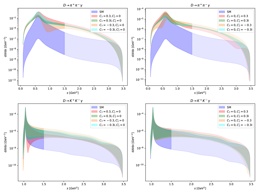
Figure 7: Comparison of QCDF-based SM predictions of differential branching ratios for $D\to\pi^{+}\pi^{-}\gamma$ (upper plots) and $D\to K^{+}K^{-}\gamma$ (lower plots) within different BSM scenarios. One BSM coefficient is set to zero while the other one exhausts the limit (43) with CP-phase $0,\pm\pi/2,\pi$.

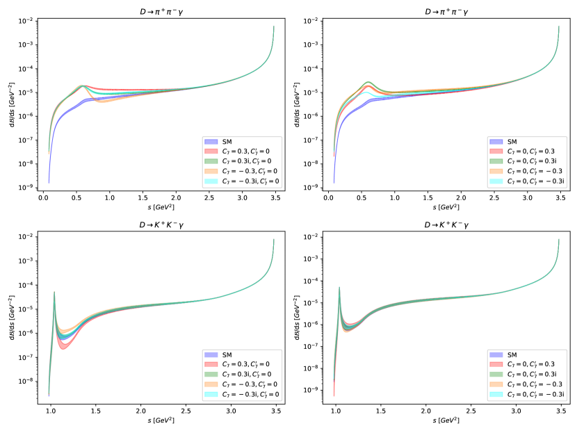
Figure 8: As in Fig. 7 but for HH$\chi$PT.

The NP impact on $A_{\rm FB}$ is sizable, see Fig. 9 for the HH$\chi$PT predictions.

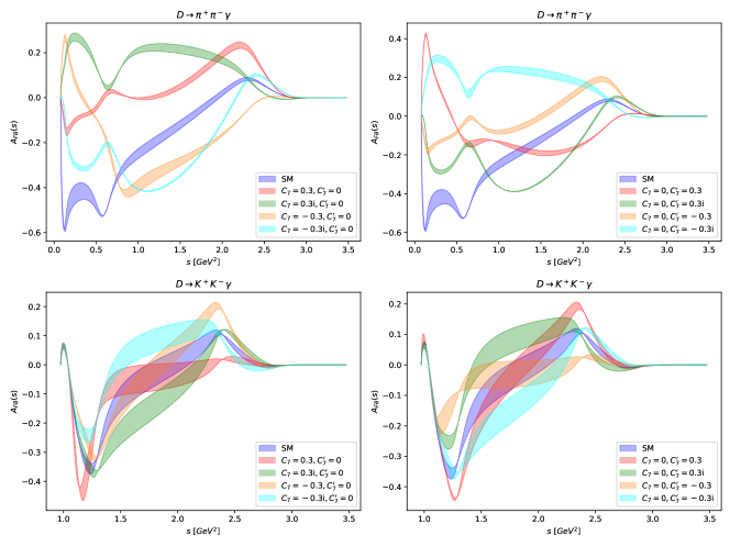
Figure 9: The forward-backward asymmetry in the SM (blue band) and beyond for the decays $D\to\pi^{+}\pi^{-}\gamma$ and $D\to K^{+}K^{-}\gamma$ as a function of $s$, based on the HH$\chi$PT form factors.

However, due to the complicated interplay of $s$-, $t$- and $u$-channel resonances further study in SM-like $D\to K\pi\gamma$ decays is suggested to understand the decay dynamics before drawing firm conclusions within NP. Since the form factors depend on $s$ and $t$, the pure BSM contributions (46) induce a forward-backward asymmetry within QCDF, whereas it vanishes in the SM (see Fig. 10).

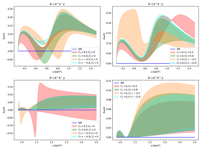
Figure 10: As in Fig. 9 but within QCDF (46).

V CP Violation

Another observable that offers the possibility to test for BSM physics is the single- or double-differential CP asymmetry. It is defined, respectively, by

$$A_{\rm CP}(s)=\int d{}tA_{\rm CP}(s,t)\,,\leavevmode\nobreak\ \leavevmode\nobreak\ \leavevmode\nobreak\ A_{\rm CP}(s,t)=\frac{1}{\Gamma+\overline{\Gamma}}\left(\frac{d{}^{2}\Gamma}{d{}sd{}t}-\frac{d{}^{2}\overline{\Gamma}}{d{}sd{}t}\right)\,.$$ (47)

Here, $\overline{\Gamma}$ refers to the decay rate of the CP-conjugated mode. Within the SM, $D\to K^{+}K^{-}\gamma$ is the only decay that contains contributions with different weak phases and thus the only decay mode with a nonvanishing CP asymmetry. A maximum of $A^{\text{SM}}_{\rm CP}(s)\lesssim 1.4\cdot 10^{-4}$ located around the $\phi$ peak is predicted by QCDF. Since the $\phi$ is a narrow resonance, the CP asymmetry decreases rapidly with increasing $s$. BSM contributions can contain further strong and weak phases and thus significantly increase the CP asymmetry. In Fig. 11 we show the predictions for the CP asymmetries within the SM and for several different BSM scenarios, based on QCDF. We assign a non-zero value to one of the BSM coefficients and set the weak phase to $\phi_{w}=\pm\pi/2$. The BSM CP asymmetries $A_{\rm CP}(s)$ can, in principle, reach $\mathcal{O}(1)$ values. Constraints can arise from data on CP asymmetries in hadronic decays; these are further discussed in Section V.1. We emphasize that $A_{\rm CP}$ depends on cuts used in the normalization $\Gamma+\bar{\Gamma}$. In Fig. 11 we include the contributions up to $s=1.5\leavevmode\nobreak\ {\rm GeV}^{2}$.

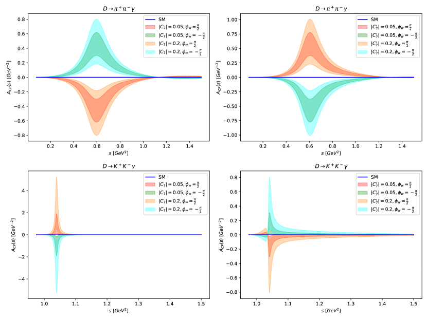
Figure 11: Predictions for the CP asymmetries in $D\to\pi^{+}\pi^{-}\gamma$ and $D\to K^{+}K^{-}\gamma$ as a function of $s$, within the SM and beyond (using (46)), based on QCDF. For the BSM scenarios, we have set one coefficient $C_{7}^{(\prime)}$ to 0 and the other one to $0.05,0.2$. The weak phase of $C_{7}^{(\prime)}$ is $\phi_{w}=\pm\pi/2$. We performed a cut $s\leq 1.5\,{\rm GeV}^{2}$ to remain within the region where QCDF applies.

HH$\chi$PT predicts a SM CP asymmetry $A_{\rm CP}^{\text{SM}}(s)\lesssim 0.7\cdot 10^{-4}$ for the $D\to K^{+}K^{-}\gamma$ decay. In Fig. 12 we show the same BSM benchmarks as before, employing HH$\chi$PT. We performed a cut $s\leq 2\,{\rm GeV}$ to avoid large bremsstrahlung effects in the normalization, which would artificially suppress $A_{\rm CP}$. Still, the CP asymmetries obtained using HH$\chi$PT are smaller than those using QCDF, since a larger part of the phase space is included in the normalization.

For $D\to\pi^{+}\pi^{-}\gamma$, the contributions of $\mathcal{A}_{-}$ and $\mathcal{A}_{+}$ to the CP asymmetries are of roughly the same size. Therefore, the relative signs of the dipole Wilson coefficients in (46) results in a constructive increase (for $C_{7}^{\prime}$) and a cancellation (for $C_{7}$), respectively, of the CP asymmetry. For the $D\to K^{+}K^{-}\gamma$ mode, the $\phi$ resonance contributes only to $A_{+}$. Therefore, in this case the CP asymmetry is dominated by the parity-even amplitude.

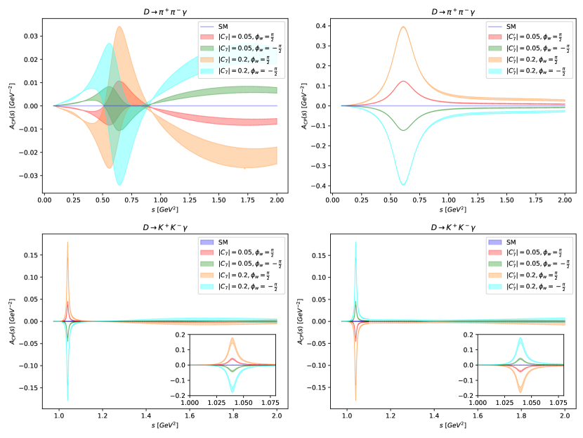
Figure 12: As in Fig. 11 but for HH$\chi$PT and with cut $s\leq 2\,{\rm GeV}^{2}$ to avoid large bremsstrahlung contributions in the normalization.

In order to get additional strong phases and thus an increase of the CP asymmetry, one could consider further heavy vector resonances such as the $\phi(1680)$. Intermediate scalar particles like $f_{0}(1710)$ Soni:2019xko would also add additional strong phases. We remark that $A_{\rm CP}$ can change its sign in dependence of $s$; therefore, binning is required to avoid cancellations. $A_{\rm CP}$ is very small beyond the $(P_{1}P_{2})_{\text{res}}$ peak due to the cancellation of the $(P_{1}\gamma)_{\text{res}}$ and $(P_{2}\gamma)_{\text{res}}$ contributions upon integration over $t$. To avoid this cancellation one could use the $s$- and $t$-dependent CP asymmetry $A_{\rm CP}(s,t)$ as shown in Fig. 13. Note that part of the resonance contribution to the asymmetry is removed by the bremsstrahlung cut.

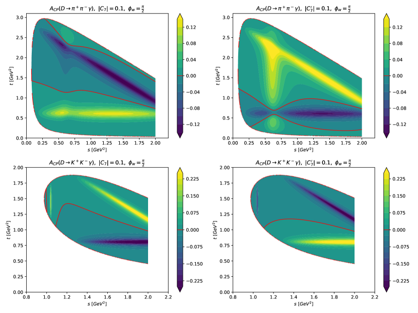
Figure 13: Dalitz plot of $A_{\rm CP}(s,t)$ for $D\to\pi^{+}\pi^{-}\gamma$ (upper plots) and $D\to K^{+}K^{-}\gamma$ decays (lower plots) based on HH$\chi$PT. We have set one BSM coefficient, $C_{7}$ or $C_{7}^{\prime}$, to 0 and the other one to $0.1$, with weak phase $\phi_{w}=\pi/2$. We employed a cut $s\leq 2\,{\rm GeV}^{2}$ to avoid large bremsstrahlung contributions in the normalization.

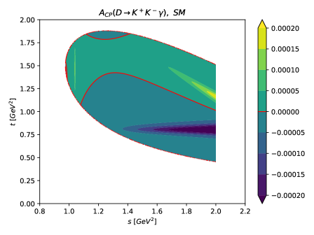
Figure 14: Dalitz plot of $A_{\rm CP}^{\rm SM}(s,t)$ for $D\to K^{+}K^{-}\gamma$ decays based on HH$\chi$PT for $s\leq 2\,{\rm GeV}^{2}$.

V.1 CP phases and $\Delta A_{\rm CP}$

We briefly discuss the impact of the chromomagnetic dipole operators $O_{8}^{(\prime)}$ on radiative charm decays, where

$$O_{8}=\frac{g_{s}m_{c}}{16\pi^{2}}\left(\overline{u}_{L}\sigma^{\mu\nu}G_{\mu\nu}c_{R}\right)\,,\qquad O_{8}^{\prime}=\frac{g_{s}m_{c}}{16\pi^{2}}\left(\overline{u}_{R}\sigma^{\mu\nu}G_{\mu\nu}c_{L}\right)\,,$$ (48)

and $G_{\mu\nu}$ denotes the chromomagnetic field strength tensor. We do not consider contributions from $O_{8}^{(\prime)}$ to the matrix element of $D\to PP\gamma$ decays, which is beyond the scope of this work. The corresponding contributions for the $D\to V\gamma$ decays have been worked out in Ref. deBoer:2017que .

The QCD renormalization-group evolution connects the electromagnetic and the chromomagnetic dipole operators at different scales. To leading order we find the following relation deBoer:2017que ,

$$C_{7}^{(\prime)}(m_{c})\simeq 0.4\big{(}C_{7}^{(\prime)}(\Lambda)-C_{8}^{(\prime)}(\Lambda)\big{)}\,,\qquad C_{8}^{(\prime)}(m_{c})\simeq 0.4C_{8}^{(\prime)}(\Lambda)\,,$$ (49)

which is valid to roughly 20% if $\Lambda$, the scale of NP, lies within 1-10 TeV. It follows that CP asymmetries for radiative decays are related to hadronic decays, a connection discussed in Isidori:2012yx ; Lyon:2012fk in the context of $\Delta A_{\rm CP}=A_{\rm CP}(D\to K^{+}K^{-})-A_{\rm CP}(D\to\pi^{+}\pi^{-})$. The latter is measured by LHCb, $\Delta A_{\rm CP}=-(15.4\pm 2.9)\cdot 10^{-4}$ Aaij:2019kcg , and implies $\Delta A_{\rm CP}^{\rm NP}\sim{\rm Im}(C_{8}-C_{8}^{\prime})\sin\delta\lesssim 2\cdot 10^{-3}$ for NP from dipole operators, with a strong phase difference $\delta$ and Wilson coefficients evaluated at $\mu=m_{c}$. For $\sin\delta\sim O(1)$, and $C_{8}$ only (or $C_{8}^{\prime}$ only), strong constraints on the electromagnetic dipole operators follow from (49), unless $C_{7}(\Lambda)\gg C_{8}(\Lambda)$, as ${\rm Im}\,C_{7}\simeq{\rm Im}\,C_{8}\lesssim 2\cdot 10^{-3}$. We study the corresponding CP asymmetries for $D\to PP\gamma$ in the Dalitz region as this avoids large cancellations from $t$- or $u$-channel resonances. Note that the latter have not been included in Ref. Isidori:2012yx . We find values of $A_{\rm CP}(s,t)$ up to $\sim(3-4)\times 10^{-3}$ which is more than one order of magnitude above the SM with maximal values of $\sim 2\times 10^{-4}$, shown in Fig. 14 for $D\to K^{+}K^{-}\gamma$. (As already discussed, the corresponding SM asymmetry for $D\to\pi^{+}\pi^{-}\gamma$ vanishes at this order.) The largest values for $A_{\rm CP}(s,t)$ arise around the resonances, notably the $K^{*}\to K\gamma$ contributions to $D\to KK\gamma$.

The BSM CP asymmetries scale linearly with ${\rm Im}\,C_{7}^{(\prime)}$. We checked explicitly that the CP asymmetries for ${\rm Im}\,C_{7}^{(\prime)}\simeq 2\cdot 10^{-3}$ agree, up to an overall suppression factor of 50, with those shown in Fig. 13 which are based on ${\rm Im}\,C_{7}^{(\prime)}\simeq 0.1$, and are therefore not shown.

Note that the $\Delta A_{\rm CP}$ constraint can be eased with a strong phase suppression. In general, it can be escaped in the presence of different sources of BSM CP violation in the hadronic amplitudes. Yet, our analysis has shown that even with small CP violation in the dipole couplings sizable NP enhancements can occur.

VI Conclusions

We worked out predictions for $D\to PP\gamma$ decay rates and asymmetries in QCDF and in HH$\chi$PT. The $D\to\pi^{+}\pi^{-}\gamma$ and $D\to K^{+}K^{-}\gamma$ decays are sensitive to BSM physics, while $D\to K\pi\gamma$ decays are SM-like and serve as “standard candles”. Therefore, a future measurement of the $D\to K\pi\gamma$ decay spectra can diagnose the performance of the QCD tools. The forward-backward asymmetry (38) is particularly useful as it vanishes for amplitudes without $t$- or $u$-channel dependence; this happens, for instance, in leading-order QCDF. On the other hand, $t$- or $u$-channel resonances are included within HH$\chi$PT, and give rise to finite interference patterns, shown in Fig. 4. Within QCDF, the value of $\tilde{C}/\lambda_{D}$ can be extracted from the branching ratio.

While branching ratios of $D\to\pi^{+}\pi^{-}\gamma$ can be affected by NP, these effects will be difficult to discern due to the large uncertainties. On the other hand, the SM can be cleanly probed with CP asymmetries in the $D\to\pi^{+}\pi^{-}\gamma$ and $D\to K^{+}K^{-}\gamma$ decays, which can be sizable, see Figs. 11 and 12. We stress that the sensitivity of the CP asymmetries is maximized by performing a Dalitz analysis or applying suitable cuts in $t$ (see Fig. 13), as otherwise large cancellations occur. Values of the CP asymmetries depend strongly on the cut in $s$ employed to remove the bremsstrahlung contribution. The latter is SM-like and dominates the branching ratios for small photon energies. The forward-backward asymmetries also offer SM tests, see Fig. 9, but requires prior consolidation of resonance effects.

Radiative charm decays are well-suited for investigation at the $e^{+}e^{-}$ flavor facilities Belle II Kou:2018nap , BES III Ablikim:2019hff , and future $e^{+}e^{-}$-colliders running at the $Z$-pole Abada:2019lih . Branching ratios for $D^{0}\to\pi^{+}\pi^{-}\gamma$ and $D^{0}\to K^{+}K^{-}\gamma$ decays are of the order $10^{-5}$, see Table 1. With fragmentation fraction $f(c\to D^{0})\simeq 0.59$ and $c\bar{c}$ production rates of $550\cdot 10^{9}$ (Fcc-ee) and $65\cdot 10^{9}$ (Belle II with $50{\rm ab}^{-1}$) Abada:2019lih this gives $6\cdot 10^{11}$ and $8\cdot 10^{10}$ neutral $D$-mesons and sizeable (unreconstructed) event rates of $6\cdot 10^{6}$ and $8\cdot 10^{5}$, respectively. Rates for the “standard candles” $D^{0}\to\pi^{+}K^{-}\gamma$ are one order of magnitude larger. We look forward to future investigations.

Appendix A Parameters

The couplings, masses, branching ratios, total decay widths and the mean life time are taken from the PDG Tanabashi:2018oca . The mass of the $\eta_{8}$ results from the Gell-Mann-Okubo (GMO) mass formula Okubo:1962 ; Gell-Mann:1964

$$m_{\eta_{8}}=\sqrt{\frac{4m_{K}^{2}-m_{\pi}^{2}}{3}}=0.56929{\rm GeV}\,.$$

The CKM matrix elements are taken from the UTfit collaboration UTfit

$$V_{ud} =0.97431\pm 0.00012,\quad\quad V_{us}=0.22514\pm 0.00055,$$

$$V_{cd} =(-0.22500\pm 0.00054)\exp\left[\mathrm{i}(0.0351\pm 0.0010)^{\circ}\right],$$

$$V_{cs} =(0.97344\pm 0.00012)\exp\left[\mathrm{i}(-0.001880\pm 0.000055)^{\circ}\right].$$

The decay constant of the D-meson is given by the FLAG working group Aoki:2016frl

$$f_{D}=(0.21215\pm 0.00145){\rm GeV}, f_{D_{s}}=(0.24883\pm 0.00127){\rm GeV},$$

$$f_{K}=(0.1556\pm 0.0004){\rm GeV}, f_{\pi}=(0.1302\pm 0.0014){\rm GeV}.$$

The $q\overline{q}-s\overline{s}$ mixing scheme Feldmann:1998vh and $\chi$PT Leutwyler:1997yr provide decay constants for $\eta_{8}$ and $\eta_{0}$

$$f_{\eta_{8}}=\sqrt{\frac{4}{3}f_{K}^{2}-\frac{1}{3}f_{\pi}^{2}}=(0.1632\pm 0.0006){\rm GeV}\,,$$

$$f_{\eta_{0}}=\sqrt{\frac{2}{3}f_{K}^{2}+\frac{1}{3}f_{\pi}^{2}}=(0.1476\pm 0.0005){\rm GeV}\,.$$

These values are in agreement with values extracted from $\eta^{(\prime)}\to\gamma\gamma$ decays Feldmann:1998vh

$$f_{\eta_{8}}=(0.164\pm 0.006){\rm GeV}\,,f_{\eta_{0}}=(0.152\pm 0.004){\rm GeV}\,.$$

The decay constants of the vector mesons are given by f_vector1 ; f_vector2 (and references therein)

$$f_{\rho}=(0.213\pm 0.005){\rm GeV} f_{\omega}=(0.197\pm 0.008){\rm GeV},$$

$$f_{\Phi}=(0.233\pm 0.004){\rm GeV}, f_{K^{*}}=(0.204\pm 0.007){\rm GeV}.$$

Appendix B Form factors

B.1 Vacuum $\to PP$ transition form factors

The electromagnetic pion form factor $F_{\pi}^{\text{em}}$ is defined as

$$\braket{\pi^{+}(p_{1})\pi^{-}(p_{2})}{j^{\text{em}}_{\mu}}{0}=(p_{1}-p_{2})_{\mu}F_{\pi}^{\text{em}}(s)\,,$$ (50)

with the electromagnetic current

$$\begin{split}j_{\mu}^{\text{em}}&=\frac{2}{3}\overline{u}\gamma_{\mu}u-\frac{1}{3}\overline{d}\gamma_{\mu}d-\frac{1}{3}\overline{s}\gamma_{\mu}s\\ &=\frac{1}{2}(\overline{u}\gamma_{\mu}u-\overline{d}\gamma_{\mu}d)+\frac{1}{6}(\overline{u}\gamma_{\mu}u+\overline{d}\gamma_{\mu}d)-\frac{1}{3}\overline{s}\gamma_{\mu}s\\ &=\frac{1}{\sqrt{2}}j_{\mu}^{(I=1)}+\frac{1}{3\sqrt{2}}j_{\mu}^{(I=0)}-\frac{1}{3}j_{\mu}^{s}\\ &=J_{\mu}^{(I=1)}+J_{\mu}^{(I=0)}+J_{\mu}^{s}\,.\end{split}$$ (51)

In the isospin symmetry limit, only the $I=1$ current contributes to $F_{\pi}^{\text{em}}$, which reads Bruch:2004py

$$F_{\pi}^{\text{em}}(s)=\left[\sum_{n=0}^{3}c_{n}BW_{n}^{KS}(s)\right]_{fit}+\left[\sum_{n=4}^{\infty}c_{n}BW_{n}^{KS}(s)\right]_{dual-QCD_{N_{C}=\infty}},$$ (52)

where the coefficients $c_{n}$ are given by

$$\begin{split}c_{0}&=1.171\pm 0.007,\quad c_{1}=-0.119\pm 0.011,\\ c_{2}&=0.0115\pm 0.0064,\quad c_{3}=-0.0438\pm 0.02,\\ c_{n}&=\frac{2(-1)^{n}\Gamma(1.8)m_{\rho}^{2}}{\sqrt{\pi}m_{n}^{2}\Gamma(n+1)\Gamma(1.3-n)}\qquad n\geq 4,\\ m_{n}^{2}&=m_{\rho}^{2}(1+2n)\end{split}$$ (53)

and the functions $BW_{n}^{KS}(s)$ read

$$\begin{split}BW_{n}^{KS}(s)&=\frac{m_{n}^{2}}{m_{n}^{2}-s-\mathrm{i}\sqrt{s}\Gamma_{n}(s)},\\ \Gamma_{n}(s)&=\frac{0.2m_{n}^{3}}{s}\left(\frac{p(s)}{p(m_{n}^{2})}\right)^{3},\\ p(s)&=0.5\sqrt{s-4m_{\pi}^{2}}.\end{split}$$ (54)

The masses and widths of the $\rho$ meson and its first resonance are fitted as well

$$\begin{split}&m_{\rho}=(0.7739\pm 0.0006){\rm GeV},\quad m_{\rho^{\prime}}=(1.357\pm 0.018){\rm GeV},\\ &\Gamma_{\rho}=(0.1149\pm 0.0010){\rm GeV},\quad\Gamma_{\rho^{\prime}}=(0.437\pm 0.060){\rm GeV}.\end{split}$$ (55)

$F_{\pi}^{\text{em}}$ is shown in Figure 15.

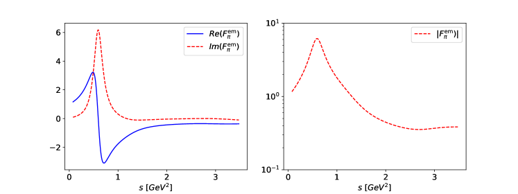
Figure 15: The real and imaginary part of the electromagnetic form factor $F_{\pi}^{\text{em}}$ (52) (left) as well as the absolute value (right) as a function of the invariant mass squared $s$.

The electromagnetic kaon form factor $F_{K^{+}}^{\text{em}}$, defined as

$$\braket{K^{+}(p_{1})K^{-}(p_{2})}{j^{\text{em}}_{\mu}}{0}=(p_{1}-p_{2})_{\mu}F_{K^{+}}^{\text{em}}(s)\,,$$ (56)

is taken from Bruch:2004py and shown in Figure 16. It can be decomposed into an isospin-one component $F_{K^{+}}^{(I=1)}$ and two isospin-zero components $F_{K^{+}}^{(I=0)}$, $F_{K^{+}}^{s}$, with $\omega$ and $\phi$ contributions, respectively,

$$\begin{split}F_{K^{+}}^{\text{em}}(s)&=F_{K^{+}}^{(I=1)}(s)+F_{K^{+}}^{(I=0)}(s)+F_{K^{+}}^{s}(s),\\ F_{K^{+}}^{(I=1)}(s)&=\frac{1}{2}(c_{\rho}^{K}BW_{\rho}(s)+c_{\rho^{\prime}}^{K}BW_{\rho^{\prime}}(s)+c_{\rho^{\prime\prime}}^{K}BW_{\rho^{\prime\prime}}(s)),\\ F_{K^{+}}^{(I=0)}(s)&=\frac{1}{6}(c_{\omega}^{K}BW_{\omega}(s)+c_{\omega^{\prime}}^{K}BW_{\omega^{\prime}}(s)+c_{\omega^{\prime\prime}}^{K}BW_{\omega^{\prime\prime}}(s)),\\ F_{K^{+}}^{s}(s)&=\frac{1}{3}(c_{\phi}BW_{\phi}(s)+c_{\phi^{\prime}}BW_{\phi^{\prime}}(s)).\end{split}$$ (57)

The requisite parameters are given by

$$\begin{split}&m_{\phi}=1.019372{\rm GeV},\quad m_{\phi}=1.68{\rm GeV},\quad m_{\rho^{\prime}}=1.465{\rm GeV},\\ &m_{\rho^{\prime\prime}}=1.720{\rm GeV},\quad m_{\omega^{\prime}}=1.425{\rm GeV},\quad m_{\omega^{\prime\prime}}=1.67{\rm GeV},\\ &\Gamma_{\phi}=0.00436{\rm GeV},\quad\Gamma_{\phi^{\prime}}=0.150{\rm GeV},\quad\Gamma_{\rho}=0.150{\rm GeV},\quad\Gamma_{\rho^{\prime}}=0.400{\rm GeV},\\ &\Gamma_{\rho^{\prime\prime}}=0.250{\rm GeV},\quad\Gamma_{\omega}=0.0084{\rm GeV},\quad\Gamma_{\omega^{\prime}}=0.215{\rm GeV},\quad\Gamma_{\omega^{\prime\prime}}=0.315{\rm GeV},\\ &c_{\phi}=(1.018\pm 0.006),\quad c_{\phi^{\prime}}=(-0.018\pm 0.006),\\ &c^{K}_{\rho}=(1.195\pm 0.009),\quad c^{K}_{\rho^{\prime}}=(-0.112\pm 0.010),\quad c^{K}_{\rho^{\prime\prime}}=(-0.083\pm 0.019),\\ &c^{K}_{\omega}=(1.195\pm 0.009),\quad c^{K}_{\omega^{\prime}}=(-0.112\pm 0.010),\quad c^{K}_{\omega^{\prime\prime}}=(-0.083\pm 0.019).\end{split}$$ (58)

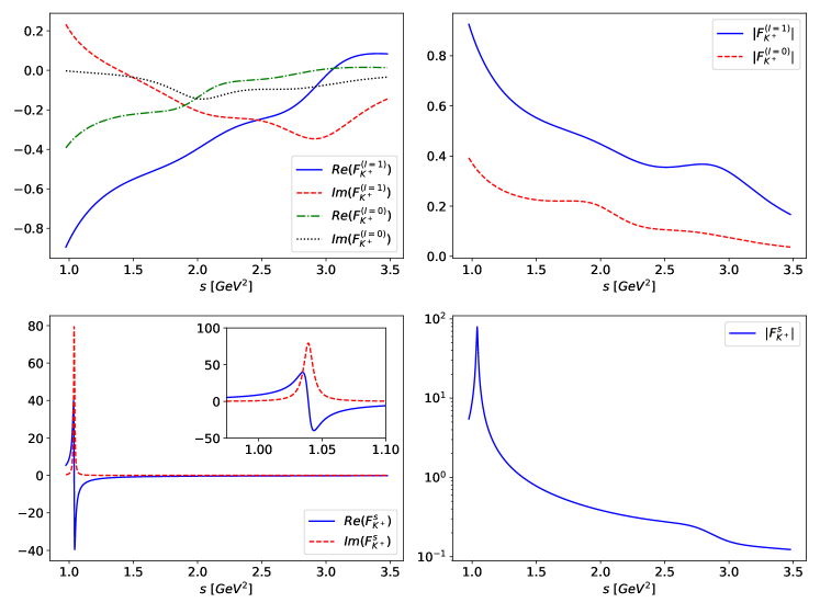
Figure 16: The real and imaginary parts of the electromagnetic kaon form factors (57) (left) as well as their absolute values (right) as a function of $s$. The upper (lower) plots show $F_{K^{+}}^{(I=1,0)}$ ($F_{K^{+}}^{s}$).

The $\overline{K}\pi^{-}$ form factors are defined as

$$\braket{\pi^{-}(p_{1})\overline{K}(p_{2})}{\overline{s}\gamma_{\mu}u}{0} =f_{+}^{\overline{K}\pi^{-}}(s)\left(p_{2}-p_{1}\right)_{\mu}+f_{-}^{\overline{K}\pi^{-}}(s)\left(p_{2}+p_{1}\right)_{\mu}$$ (59)

$$=-\frac{\Delta_{K\pi}}{s}f_{0}^{\overline{K}\pi^{-}}(s)\left(p_{2}+p_{1}\right)_{\mu}+\left[\left(p_{2}-p_{1}\right)_{\mu}+\frac{\Delta_{K\pi}}{s}\left(p_{2}+p_{1}\right)_{\mu}\right]f_{+}^{\overline{K}\pi^{-}}(s)\,,$$

with $\Delta_{K\pi}=m_{K}^{2}-m_{\pi}^{2}$. The vector form factor $f_{+}^{\overline{K}\pi^{-}}$, shown in Figure 17, can be parametrized with a dispersion relation with three subtractions at $s=0$ Boito:2008fq

$$f_{+}^{\overline{K}\pi^{-}}(s)=f_{+}^{\overline{K}\pi^{-}}(0)\cdot\exp\left[\lambda_{+}^{\prime}\frac{s}{m_{\pi}^{2}}+\frac{1}{2}\left(\lambda_{+}^{\prime\prime}-\lambda_{+}^{\prime 2}\right)\frac{s}{m_{\pi}^{4}}+\frac{s^{3}}{\pi}\int_{s_{K\pi}}^{s_{cut}}d{}s^{\prime}\frac{\delta_{1}^{K\pi}(s^{\prime})}{(s^{\prime})^{3}(s^{\prime}-s-\mathrm{i}\epsilon)}\right]\,,$$ (60)

with $s_{K\pi}=(m_{K}+m_{\pi})^{2}$. The phase $\delta_{1}^{K\pi}(s)$ is extracted from a two resonance model Boito:2008fq

$$\tilde{f}_{+}^{\overline{K}\pi^{-}}(s)=\frac{f_{+}^{\overline{K}\pi^{-}}(s)}{f_{+}^{\overline{K}\pi^{-}}(0)}=\frac{m^{2}_{K^{\star}}-\kappa_{K^{\star}}\tilde{H}_{K\pi}(0)+\beta s}{D(K^{\star})}-\frac{\beta s}{D(K^{\star\prime})}\,,$$ (61)

where

$$\begin{split}&D(n)=m_{n}^{2}-s-\kappa_{n}\text{Re}\left(\tilde{H}_{K\pi}(s)\right)-\mathrm{i}m_{n}\gamma_{n}(s)\,,\\ &\gamma_{n}(s)=\gamma_{n}\frac{s}{m_{n}^{2}}\frac{\sigma_{K\pi}^{3}(s)}{\sigma_{K\pi}^{3}(m_{n}^{2})},\qquad\gamma_{n}=\gamma_{n}(m_{n}^{2})\,,\\ &\sigma_{K\pi}(s)=\frac{2q_{K\pi}(s)}{\sqrt{s}}=\frac{1}{s}\sqrt{\left(s-(m_{K}+m_{\pi})^{2}\right)\left(s-(m_{K}-m_{\pi})^{2}\right)}\,,\\ &\kappa_{n}=\frac{192\pi f_{K}f_{\pi}}{\sigma^{3}_{K\pi}(m_{n}^{2})}\frac{\gamma_{n}}{m_{n}}\,.\end{split}$$ (62)

The function $\tilde{H}_{K\pi}$ is a $\chi$PT loop integral function Jamin:2006tk

$$\tilde{H}_{K\pi}(s)=H_{K\pi}(s)-\frac{2}{3f_{\pi}^{2}}L_{K\pi}^{r}s=\frac{1}{f_{\pi}^{2}}\left[sM_{K\pi}^{r}(s)-L_{K\pi}(s)\right]\,;$$ (63)

explicit expressions for $M^{r}(s)$ and $L(s)$ can be found in chapter 8 of Ref. Gasser1985 :

$$\begin{split}&M_{K\pi}^{r}(s)=\frac{1}{12s}(s-2\Sigma)\overline{J}_{K\pi}(s)+\frac{\Delta^{2}}{3s^{2}}\overline{\overline{J}}_{K\pi}(s)-\frac{1}{6}k_{K\pi}(\mu)+\frac{1}{288\pi^{2}}\,,\\ &L_{K\pi}(s)=\frac{\Delta^{2}}{4s}\overline{J}_{K\pi}(s)\,,\\ &k_{K\pi}(\mu)=\frac{1}{32\pi^{2}}\frac{1}{\Delta}\left(m_{K}^{2}\ln\left(\frac{m_{K}^{2}}{\mu^{2}}\right)-m_{\pi}^{2}\ln\left(\frac{m_{\pi}^{2}}{\mu^{2}}\right)\right)\,,\\ &\overline{\overline{J}}_{K\pi}(s)=\overline{J}_{K\pi}(s)-s\overline{J}_{K\pi}^{\prime}(0)\,,\\ &\overline{J}_{K\pi}(s)=J_{K\pi}(s)-J_{K\pi}(0)\\ &\qquad\quad=\frac{1}{32\pi^{2}}\left(2+\left[\frac{\Delta}{s}-\frac{\Sigma}{\Delta}\right]\ln\left(\frac{m_{\pi}^{2}}{m_{K}^{2}}\right)-\frac{v}{s}\ln\left(\frac{(s+v)^{2}-\Delta^{2}}{(s-v)^{2}-\Delta^{2}}\right)\right)\,,\\ &\overline{J}_{K\pi}^{\prime}(0)=\frac{1}{32\pi^{2}}\left(\frac{\Sigma}{\Delta^{2}}+2\frac{m_{K}^{2}m_{\pi}^{2}}{\Delta^{3}}\ln\left(\frac{m_{\pi}^{2}}{m_{K}^{2}}\right)\right)\,,\\ &v(s)=s\sigma_{K\pi}(s)\,,\\ &\Sigma=m_{K}^{2}+m_{\pi}^{2}\,,\\ &\Delta=m_{K}^{2}-m_{\pi}^{2}\,.\end{split}$$ (64)

The renormalization scale $\mu$ is set to the physical resonance mass $\mu=m_{K^{\star}}$ Boito:2008fq . The resonance masses and width parameters are unphysical fitting parameters. They are obtained as Boito:2008fq

$$\begin{split}&m_{K^{\star}}^{\text{fit}}=(0.94341\pm 0.00058){\rm GeV}\,,\qquad\gamma_{K^{\star}}^{\text{fit}}=(0.06672\pm 0.00086){\rm GeV}\,,\\ &m_{K^{\star\prime}}^{\text{fit}}=(1.374\pm 0.030){\rm GeV}\,,\qquad\gamma_{K^{\star\prime}}^{\text{fit}}=(0.24\pm 0.10){\rm GeV}\,,\\ &s_{cut}=4{\rm GeV}^{2}\,,\qquad\mu=m^{\text{phy}}_{K\star}=0.892{\rm GeV}\,,\qquad\beta=(-3.9\pm 1.5)\cdot 10^{-2}\,,\\ &\lambda_{+}^{\prime}=(24.66\pm 0.69)\cdot 10^{-3}\,,\qquad\lambda_{+}^{\prime\prime}=(11.99\pm 0.19)\cdot 10^{-4}\,,\\ &|V_{us}|f_{+}^{\overline{K}\pi^{-}}(0)=0.21664\pm 0.00048\,.\end{split}$$ (65)

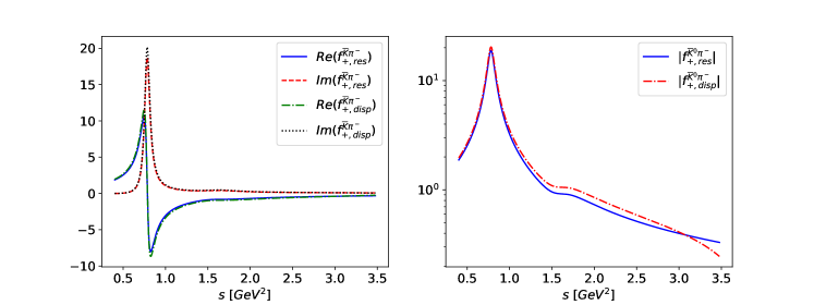
Figure 17: The real and imaginary part (left) of the $f_{+}^{\overline{K}\pi^{-}}$ form factor (59) as well as the absolute value (right) versus $s$ in the two resonance models as well as in the dispersive description. The form factor is extracted from $\tau^{-}\rightarrow\nu_{\tau}K_{s}\pi^{-}$ decays Boito:2008fq . For $\bar{K}^{0}\pi^{0}$ and $K^{+}\pi^{-}$, we use isospin relations (11).

B.2 HH$\chi$PT form factors

B.2.1 Vector form factors

Figure 18: Feynman diagrams for the $D\to\pi^{+}K^{-}\gamma$ decay, which contribute to the parity-even form factors $A$ and $E$. The diagrams for the decays $D\to\pi^{+}\pi^{-}\gamma$ and $D\to K^{+}K^{-}\gamma$ are obtained by adjusting the flavors. We have added the diagrams $E_{1,2}$ and $E_{2,2}$ (see Fajfer:2002bq ) to make the amplitude E gauge invariant for any choice of a. Additionally, for each of the diagrams $A_{1,1}$, $A_{1,2}$, $A_{1,3}$, $A_{2,2}$, $A_{2,3}$, $A_{2,4}$, $E_{1,1}$, $E_{1,2}$, $E_{1,3}$, $E_{2,1}$ and $E_{2,3}$ there is another one where the photon is coupled via a vector meson.

Figure 19: Feynman diagrams for the $D\to\pi^{+}K^{-}\gamma$ decay, which contribute to the parity-odd form factors $B$ and $D$. The diagrams for the decays $D\to\pi^{+}\pi^{-}\gamma$ and $D\to K^{+}K^{-}\gamma$ are obtained by adjusting the flavors.

$D\to\pi^{0}\overline{K}\gamma$

$$\begin{split}E_{1}^{(d,s)}&=\mathrm{i}g\frac{f_{D}f_{K}}{f_{\pi}}\frac{v\cdot k}{v\cdot k+v\cdot p_{1}+\Delta}\left(\frac{1}{v\cdot k+\Delta}-\frac{1}{v\cdot p_{1}+\Delta}\right)\left(\sqrt{2}\lambda^{\prime}+\frac{1}{2}\lambda g_{v}\left(\frac{g_{\omega}}{3m_{\omega}^{2}}+\frac{g_{\rho}}{m_{\rho}^{2}}\right)\right)\end{split}$$ (66)

$$\begin{split}D_{1}^{(d,s)}&=-\sqrt{2}\frac{f_{D}f_{K}}{f_{\pi}}\lambda^{\prime}\left(\frac{1}{v\cdot k+\Delta}+g\frac{v\cdot p_{2}}{v\cdot p_{1}+v\cdot k}\left[\frac{1}{v\cdot k+\Delta}+\frac{1}{v\cdot p_{1}+\Delta}\right]\right)\\ D_{2}^{(d,s)}&=-\frac{1}{2}\frac{f_{D}f_{K}}{f_{\pi}}\lambda g_{v}\left(\frac{g_{\omega}}{3m_{\omega}^{2}}+\frac{g_{\rho}}{m_{\rho}^{2}}\right)\left(\frac{1}{v\cdot k+\Delta}+g\frac{v\cdot p_{2}}{v\cdot p_{1}+v\cdot k}\left[\frac{1}{v\cdot k+\Delta}+\frac{1}{v\cdot p_{1}+\Delta}\right]\right)\\ D_{3}^{(d,s)}&=-\sqrt{\frac{2}{m_{D}}}f_{K}(\alpha_{1}m_{D}-\alpha_{2}v\cdot p_{2})\left(\frac{m_{\rho}^{2}g_{\rho\pi\gamma}}{g_{\rho}}BW_{\rho}(p_{1}+k)+\frac{m_{\omega}^{2}g_{\omega\pi\gamma}}{g_{\omega}}BW_{\omega}(p_{1}+k)\right)\\ &+\frac{1}{\sqrt{2}}g_{\overline{K}^{\star}}g_{\overline{K}^{\star}\overline{K}\gamma}\frac{f_{D}}{f_{\pi}}\left(1+g\frac{m_{D}-v\cdot p_{1}}{v\cdot p_{1}+\Delta}\right)BW_{\overline{K}^{\star}}(p_{2}+k)\\ D_{4}^{(d,s)}&=-f_{D}\frac{1}{v\cdot k+\Delta}\left(1-m_{K^{\star}}^{2}BW_{\overline{K}^{\star}}(p_{1}+p_{2})\right)\left(\sqrt{2}\lambda^{\prime}+\frac{1}{2}\lambda g_{v}\left(\frac{g_{\omega}}{3m_{\omega}^{2}}+\frac{g_{\rho}}{m_{\rho}^{2}}\right)\right)\\ D_{5}^{(d,s)}&=\frac{1}{\sqrt{2}}\frac{f_{D}}{f_{K}}(g_{\rho}g_{\rho\pi\gamma}BW_{\rho}(p_{1}+k)-g_{\omega}g_{\omega\pi\gamma}BW_{\omega}(p_{1}+k))\\ D_{6}^{(d,s)}&=\frac{1}{\sqrt{2}}f_{D}f_{K}\frac{m_{D}^{2}}{m_{D}^{2}-m_{K^{0}}^{2}}\left(\frac{m_{\rho}^{2}}{g_{\rho}}g_{\rho\pi\gamma}BW_{\rho}(p_{1}+k)-\frac{m_{\omega}^{2}}{g_{\omega}}g_{\omega\pi\gamma}BW_{\omega}(p_{1}+k)\right)\end{split}$$ (67)

$D\to\pi^{+}K^{-}\gamma$

$$\begin{split}A_{1}^{(d,s)}&=\mathrm{i}\frac{f_{D}f_{\pi}}{f_{K}}\frac{p_{1}\cdot k-m_{D}(v\cdot k+v\cdot p_{1})}{(p_{1}\cdot k)(p_{2}\cdot k)}\\ A_{2}^{(d,s)}&=-\mathrm{i}\sqrt{m_{D}m_{D_{s}}}\frac{f_{D_{s}}f_{\pi}}{f_{K}}\frac{g}{(p_{1}\cdot k)(p_{2}\cdot k)}\left(\frac{p_{2}\cdot k(m_{D}-v\cdot p_{2})}{m_{D}(v\cdot p_{2}+\Delta)}+\frac{p_{2}\cdot k\left[p_{1}\cdot p_{2}-(v\cdot p_{1})(v\cdot p_{2})\right]}{m_{D}(v\cdot p_{2}+\Delta)(v\cdot p_{2}+v\cdot k+\Delta)}\right.\\ &+\left.\frac{(m_{D}-v\cdot p_{1})p_{1}\cdot k+m_{D}p_{1}\cdot p_{2}+m_{D}(v\cdot p_{1})(v\cdot p_{2})}{m_{D}(v\cdot p_{2}+v\cdot k+\Delta)}\right)\\ A_{3}^{(d,s)}&=\mathrm{i}\sqrt{\frac{m_{D_{s}}}{m_{D}}}\frac{f_{D_{s}}f_{\pi}}{f_{K}}g\frac{v\cdot k}{v\cdot k+v\cdot p_{2}+\Delta}\left(\frac{2\lambda^{\prime}-\frac{\sqrt{2}}{3}\lambda g_{v}\frac{g_{\Phi}}{m_{\Phi}^{2}}}{v\cdot p_{2}+\Delta}-\frac{2\lambda^{\prime}+\frac{1}{\sqrt{2}}\lambda g_{v}\left(\frac{g_{\omega}}{3m_{\omega}^{2}}+\frac{g_{\rho}}{m_{\rho}^{2}}\right)}{v\cdot k+\Delta}\right)\end{split}$$ (68)

$$\begin{split}B_{1}^{(d,s)}&=2\frac{f_{D}f_{\pi}}{f_{K}}\lambda^{\prime}\left(\frac{1}{v\cdot k+\Delta}+g\frac{f_{D_{s}}}{f_{D}}\sqrt{\frac{m_{D_{s}}}{m_{D}}}\frac{v\cdot p_{1}}{(v\cdot p_{2}+v\cdot k)}\left[\frac{1}{v\cdot k+\Delta}+\frac{1}{v\cdot p_{2}+\Delta}\right]\right)\\ B_{2}^{(d,s)}&=\frac{1}{\sqrt{2}}\frac{f_{\pi}}{f_{K}}\lambda g_{v}\left(\frac{g_{\omega}}{3m_{\omega}^{2}}+\frac{g_{\rho}}{m_{\rho}^{2}}\right)\frac{1}{v\cdot k+\Delta}\left(f_{D}+g\sqrt{\frac{m_{D_{s}}}{m_{D}}}f_{D_{s}}\frac{v\cdot p_{1}}{(v\cdot p_{2}+v\cdot k)}\right)\\ &-g\lambda g_{v}\sqrt{\frac{m_{D_{s}}}{m_{D}}}\frac{f_{D_{s}}f_{\pi}}{f_{K}}\frac{\sqrt{2}g_{\Phi}}{3m_{\Phi}^{2}}\frac{v\cdot p_{1}}{(v\cdot p_{2}+v\cdot k)(v\cdot p_{2}+\Delta)}\\ B_{3}^{(d,s)}&=\frac{2}{\sqrt{m_{D}}}f_{\pi}\frac{m^{2}_{K^{\star}}g_{K^{\star\pm}K^{\pm}\gamma}}{g_{K^{\star}}}(\alpha_{1}m_{D}-\alpha_{2}v\cdot p_{1})BW_{K^{\star-}}(p_{2}+k)\\ &-g_{\rho}g_{\rho^{\pm}\pi^{\pm}\gamma}\frac{f_{D}}{f_{K}}\left(1+g\sqrt{\frac{m_{D_{s}}}{m_{D}}}\frac{f_{D_{s}}}{f_{D}}\frac{m_{D}-v\cdot p_{2}}{v\cdot p_{2}+\Delta}\right)BW_{\rho^{+}}(p_{1}+k)\end{split}$$ (69)

$$\begin{split}D_{1}^{(d,s)}&=\frac{f_{D}}{v\cdot k+\Delta}\left(1-m_{K^{\star}}^{2}BW_{\overline{K}^{\star}}(p_{1}+p_{2})\right)\left(2\lambda^{\prime}+\frac{1}{\sqrt{2}}\lambda g_{v}\left(\frac{g_{\omega}}{3m_{\omega}^{2}}+\frac{g_{\rho}}{m_{\rho}^{2}}\right)\right)\\ D_{2}^{(d,s)}&=-\frac{f_{D}}{f_{\pi}}g_{K^{\star}}g_{K^{\star\pm}K^{\pm}\gamma}BW_{K^{\star-}}(p_{2}+k)-\frac{f_{D}}{f_{K}}g_{\rho}g_{\rho^{\pm}\pi^{\pm}\gamma}BW_{\rho^{+}}(p_{1}+k)\\ D_{3}^{(d,s)}&={f_{D}f_{K}}\frac{m_{D}^{2}}{m_{D}^{2}-m_{K^{0}}^{2}}\left(\frac{m_{\rho}^{2}}{g_{\rho}}g_{\rho^{\pm}\pi^{\pm}\gamma}BW_{\rho^{+}}(p_{1}+k)+\frac{m_{K^{\star}}^{2}}{g_{K^{\star}}}g_{K^{\star\pm}K^{\pm}\gamma}BW_{K^{\star-}}(p_{2}+k)\right)\end{split}$$ (70)

$D\to\pi^{+}\pi^{-}\gamma$

$$\begin{split}A_{1}^{(d,d)}&=\mathrm{i}f_{D}\frac{p_{1}\cdot k-m_{D}(v\cdot k+v\cdot p_{1})}{(p_{1}\cdot k)(p_{2}\cdot k)}\\ A_{2}^{(d,d)}&=-\mathrm{i}m_{D}f_{D}\frac{g}{(p_{1}\cdot k)(p_{2}\cdot k)}\left(\frac{p_{2}\cdot k(m_{D}-v\cdot p_{2})}{m_{D}(v\cdot p_{2}+\Delta)}+\frac{p_{2}\cdot k\left[p_{1}\cdot p_{2}-(v\cdot p_{1})(v\cdot p_{2})\right]}{m_{D}(v\cdot p_{2}+\Delta)(v\cdot p_{2}+v\cdot k+\Delta)}\right.\\ &+\left.\frac{(m_{D}-v\cdot p_{1})p_{1}\cdot k+m_{D}p_{1}\cdot p_{2}+m_{D}(v\cdot p_{1})(v\cdot p_{2})}{m_{D}(v\cdot p_{2}+v\cdot k+\Delta)}\right)\\ A_{3}^{(d,d)}&=\mathrm{i}f_{D}g\frac{v\cdot k}{v\cdot k+v\cdot p_{2}+\Delta}\left(\frac{2\lambda^{\prime}+\frac{1}{\sqrt{2}}\lambda g_{v}\left(\frac{g_{\omega}}{3m_{\omega}^{2}}-\frac{g_{\rho}}{m_{\rho}^{2}}\right)}{v\cdot p_{2}+\Delta}-\frac{2\lambda^{\prime}+\frac{1}{\sqrt{2}}\lambda g_{v}\left(\frac{g_{\omega}}{3m_{\omega}^{2}}+\frac{g_{\rho}}{m_{\rho}^{2}}\right)}{v\cdot k+\Delta}\right)\end{split}$$ (71)

$$\begin{split}B_{1}^{(d,d)}&=2f_{D}\lambda^{\prime}\left(\frac{1}{v\cdot k+\Delta}+g\frac{v\cdot p_{1}}{(v\cdot p_{2}+v\cdot k)}\left[\frac{1}{v\cdot k+\Delta}+\frac{1}{v\cdot p_{2}+\Delta}\right]\right)\\ B_{2}^{(d,d)}&=\frac{1}{\sqrt{2}}\lambda g_{v}f_{D}\left(\frac{g_{\omega}}{3m_{\omega}^{2}}+\frac{g_{\rho}}{m_{\rho}^{2}}\right)\frac{1}{v\cdot k+\Delta}\left(1+g\frac{v\cdot p_{1}}{(v\cdot p_{2}+v\cdot k)}\right)\\ &+\frac{1}{\sqrt{2}}g\lambda g_{v}f_{D}\left(\frac{g_{\omega}}{3m_{\omega}^{2}}-\frac{g_{\rho}}{m_{\rho}^{2}}\right)\frac{v\cdot p_{1}}{(v\cdot p_{2}+v\cdot k)(v\cdot p_{2}+\Delta)}\\ B_{3}^{(d,d)}&=\frac{2}{\sqrt{m_{D}}}f_{\pi}\frac{m_{\rho}^{2}}{g_{\rho}}g_{\rho^{\pm}\pi^{\pm}\gamma}(\alpha_{1}m_{D}-\alpha_{2}v\cdot p_{1})BW_{\rho^{-}}(p_{2}+k)\\ &-g_{\rho}g_{\rho^{\pm}\pi^{\pm}\gamma}\frac{f_{D}}{f_{\pi}}\left(1+g\frac{m_{D}-v\cdot p_{2}}{v\cdot p_{2}+\Delta}\right)BW_{\rho^{+}}(p_{1}+k)\end{split}$$ (72)

$$\begin{split}D_{1}^{(d,d)}&=f_{D}\frac{1}{v\cdot k+\Delta}\left(1-m_{\rho}^{2}BW_{\rho}(p_{1}+p_{2})\right)\left(2\lambda^{\prime}+\frac{1}{\sqrt{2}}\lambda g_{v}\left(\frac{g_{\omega}}{3m_{\omega}^{2}}+\frac{g_{\rho}}{m_{\rho}^{2}}\right)\right)\\ D_{2}^{(d,d)}&=-\frac{f_{D}}{f_{\pi}}g_{\rho}g_{\rho^{\star\pm}\pi^{\pm}\gamma}(BW_{\rho^{-}}(p_{2}+k)+BW_{\rho^{+}}(p_{1}+k))\\ D_{3}^{(d,d)}&={f_{D}f_{\pi}}\frac{m_{D}^{2}}{m_{D}^{2}-m_{\pi^{0}}^{2}}\frac{m_{\rho}^{2}}{g_{\rho}}g_{\rho^{\pm}\pi^{\pm}\gamma}\left(BW_{\rho^{+}}(p_{1}+k)+BW_{\rho^{-}}(p_{2}+k)\right)\end{split}$$ (73)

$D\to K^{+}K^{-}\gamma$

$$\begin{split}A_{1}^{(s,s)}&=\mathrm{i}f_{D}\frac{p_{1}\cdot k-m_{D}(v\cdot k+v\cdot p_{1})}{(p_{1}\cdot k)(p_{2}\cdot k)}\\ A_{2}^{(s,s)}&=-\mathrm{i}\sqrt{m_{D}m_{D_{s}}}f_{D_{s}}\frac{g}{(p_{1}\cdot k)(p_{2}\cdot k)}\left(\frac{p_{2}\cdot k(m_{D}-v\cdot p_{2})}{m_{D}(v\cdot p_{2}+\Delta)}+\frac{p_{2}\cdot k\left[p_{1}\cdot p_{2}-(v\cdot p_{1})(v\cdot p_{2})\right]}{m_{D}(v\cdot p_{2}+\Delta)(v\cdot p_{2}+v\cdot k+\Delta)}\right.\\ &+\left.\frac{(m_{D}-v\cdot p_{1})p_{1}\cdot k+m_{D}p_{1}\cdot p_{2}+m_{D}(v\cdot p_{1})(v\cdot p_{2})}{m_{D}(v\cdot p_{2}+v\cdot k+\Delta)}\right)\\ A_{3}^{(s,s)}&=\mathrm{i}\sqrt{\frac{m_{D_{s}}}{m_{D}}}f_{D_{s}}g\frac{v\cdot k}{v\cdot k+v\cdot p_{2}+\Delta}\left(\frac{2\lambda^{\prime}-\frac{\sqrt{2}}{3}\lambda g_{v}\frac{g_{\Phi}}{m_{\Phi}^{2}}}{v\cdot p_{2}+\Delta}-\frac{2\lambda^{\prime}+\frac{1}{\sqrt{2}}\lambda g_{v}\left(\frac{g_{\omega}}{3m_{\omega}^{2}}+\frac{g_{\rho}}{m_{\rho}^{2}}\right)}{v\cdot k+\Delta}\right)\end{split}$$ (74)

$$\begin{split}B_{1}^{(s,s)}&=2f_{D}\lambda^{\prime}\left(\frac{1}{v\cdot k+\Delta}+g\frac{f_{D_{s}}}{f_{D}}\sqrt{\frac{m_{D_{s}}}{m_{D}}}\frac{v\cdot p_{1}}{(v\cdot p_{2}+v\cdot k)}\left[\frac{1}{v\cdot k+\Delta}+\frac{1}{v\cdot p_{2}+\Delta}\right]\right)\\ B_{2}^{(s,s)}&=\frac{1}{\sqrt{2}}\lambda g_{v}\left(\frac{g_{\omega}}{3m_{\omega}^{2}}+\frac{g_{\rho}}{m_{\rho}^{2}}\right)\frac{1}{v\cdot k+\Delta}\left(f_{D}+gf_{D_{s}}\sqrt{\frac{m_{D_{s}}}{m_{D}}}\frac{v\cdot p_{1}}{(v\cdot p_{2}+v\cdot k)}\right)\\ &-g\lambda g_{v}\sqrt{\frac{m_{D_{s}}}{m_{D}}}f_{D_{s}}\frac{\sqrt{2}g_{\Phi}}{3m_{\Phi}^{2}}\frac{v\cdot p_{1}}{(v\cdot p_{2}+v\cdot k)(v\cdot p_{2}+\Delta)}\\ B_{3}^{(s,s)}&=\frac{2}{\sqrt{m_{D}}}f_{K}\frac{m^{2}_{K^{\star}}}{g_{K^{\star}}}g_{K^{\star\pm}K^{\pm}\gamma}(\alpha_{1}m_{D}-\alpha_{2}v\cdot p_{1})BW_{K^{\star-}}(p_{2}+k)\\ &-g_{K^{\star}}g_{K^{\star\pm}K^{\pm}\gamma}\frac{f_{D}}{f_{K}}\left(1+g\sqrt{\frac{m_{D_{s}}}{m_{D}}}\frac{f_{D_{s}}}{f_{D}}\frac{m_{D}-v\cdot p_{2}}{v\cdot p_{2}+\Delta}\right)BW_{K^{\star+}}(p_{1}+k)\end{split}$$ (75)

$$\begin{split}D_{1}^{(s,s)}&=f_{D}\frac{1}{v\cdot k+\Delta}\left(1-m_{\Phi}^{2}BW_{\Phi}(p_{1}+p_{2})\right)\left(2\lambda^{\prime}+\frac{1}{\sqrt{2}}\lambda g_{v}\left(\frac{g_{\omega}}{3m_{\omega}^{2}}+\frac{g_{\rho}}{m_{\rho}^{2}}\right)\right)\\ D_{1}^{(d,d)}&=f_{D}\frac{1}{v\cdot k+\Delta}\left(m_{\omega}^{2}BW_{\omega}(p_{1}+p_{2})-m_{\rho}^{2}BW_{\rho}(p_{1}+p_{2})\right)\left(\lambda^{\prime}+\frac{1}{2\sqrt{2}}\lambda g_{v}\left(\frac{g_{\omega}}{3m_{\omega}^{2}}+\frac{g_{\rho}}{m_{\rho}^{2}}\right)\right)\\ D_{2}^{(s,s)}&=-\frac{f_{D}}{f_{K}}g_{K^{\star}}g_{K^{\star\pm}K^{\pm}\gamma}\left(BW_{K^{\star+}}(p_{1}+k)+BW_{K^{\star-}}(p_{2}+k)\right)\\ D_{3}^{(s,s)}&=-\frac{f_{D}f_{\eta_{8}}}{2}\frac{m_{D}^{2}}{m_{D}^{2}-m_{\eta_{8}}^{2}}\frac{m_{K^{\star}}^{2}}{g_{K^{\star}}}g_{K^{\star\pm}K^{\pm}\gamma}\left(BW_{K^{\star+}}(p_{1}+k)+BW_{K^{\star-}}(p_{2}+k)\right)\\ D_{3}^{(d,d)}&=-\frac{f_{D}}{2}m_{D}^{2}\left(\frac{f_{\eta_{8}}}{m_{D}^{2}-m_{\eta_{8}}^{2}}+\frac{f_{\pi}}{m_{D}^{2}-m_{\pi}^{2}}\right)\frac{m_{K^{\star}}^{2}}{g_{K^{\star}}}g_{K^{\star\pm}K^{\pm}\gamma}\left(BW_{K^{\star+}}(p_{1}+k)+BW_{K^{\star-}}(p_{2}+k)\right)\end{split}$$ (76)

$$\begin{split}&BW_{n}(x)=\frac{1}{x^{2}-m_{n}^{2}+\mathrm{i}m_{n}\Gamma_{n}}\,,\\ &\Delta=m_{D^{\star}}-m_{D}\end{split}$$ (77)

B.2.2 Tensor form factors

Figure 20: Feynman diagrams contributing to the tensor current form factors $a^{\prime}$, $b^{\prime}$, $c^{\prime}$ and $h^{\prime}$.

$D\to\pi^{+}\pi^{-}$

$$\begin{split}a^{\prime}&=-\frac{g^{2}f_{D}\left(p_{2}\cdot k-(v\cdot k)(v\cdot p_{2})\right)}{f_{\pi}^{2}(v\cdot p_{2}+\Delta)(v\cdot p_{1}+v\cdot p_{2}+\Delta)}+\frac{\alpha_{1}(v\cdot k)}{f_{\pi}^{2}\sqrt{m_{D}}}\left[1+\frac{f_{\pi}^{2}m_{\rho}^{4}}{g_{\rho}^{2}}BW_{\rho}(p_{1}+p_{2})\right]\\ &-{\frac{\sqrt{2}\lambda f_{D}g_{v}}{(v\cdot p_{1}+v\cdot p_{2}+\Delta)}\frac{m_{\rho}^{2}}{g_{\rho}}\left(p_{2}\cdot k-(v\cdot k)(v\cdot p_{2})\right)BW_{\rho}(p_{1}+p_{2})}\end{split}$$ (78)

$$\begin{split}b^{\prime}&=\frac{gf_{D}}{f_{\pi}^{2}(v\cdot p_{2}+\Delta)}\left[v\cdot k+\frac{g\left(p_{1}\cdot k-(v\cdot k)(v\cdot p_{1})\right)}{(v\cdot p_{1}+v\cdot p_{2}+\Delta)}\right]-{\frac{\alpha_{1}(v\cdot k)}{f_{\pi}^{2}\sqrt{m_{D}}}}\left[{1}+{\frac{f_{\pi}^{2}m_{\rho}^{4}}{g_{\rho}^{2}}BW_{\rho}(p_{1}+p_{2})}\right]\\ &+{\frac{\sqrt{2}\lambda f_{D}g_{v}}{(v\cdot p_{1}+v\cdot p_{2}+\Delta)}\frac{m_{\rho}^{2}}{g_{\rho}}\left(p_{1}\cdot k-(v\cdot k)(v\cdot p_{1})\right)BW_{\rho}(p_{1}+p_{2})}\end{split}$$ (79)

$$\begin{split}c^{\prime}&=\frac{gf_{D}}{f_{\pi}^{2}m_{D}(v\cdot p_{2}+\Delta)}\left[-p_{2}\cdot k+\frac{g\left((p_{2}\cdot k)(v\cdot p_{1})-(p_{1}\cdot k)(v\cdot p_{2})\right)}{(v\cdot p_{1}+v\cdot p_{2}+\Delta)}\right]\\ &+{\frac{\alpha_{1}}{f_{\pi}^{2}m_{D}^{\frac{3}{2}}}(p_{2}\cdot k-p_{1}\cdot k)}\left[{1}+{\frac{f_{\pi}^{2}m_{\rho}^{4}}{g_{\rho}^{2}}BW_{\rho}(p_{1}+p_{2})}\right]\\ &-{\frac{\sqrt{2}\lambda f_{D}g_{v}}{m_{D}(v\cdot p_{1}+v\cdot p_{2}+\Delta)}\frac{m_{\rho}^{2}}{g_{\rho}}\left((p_{1}\cdot k)(v\cdot p_{2})-(p_{2}\cdot k)(v\cdot p_{1})\right)BW_{\rho}(p_{1}+p_{2})}\end{split}$$ (80)

$$\begin{split}h^{\prime}&=\frac{gf_{D}}{2f_{\pi}^{2}m_{D}(v\cdot p_{2}+\Delta)}\left[1+\frac{gv\cdot k}{(v\cdot p_{1}+v\cdot p_{2}+\Delta)}\right]+{\frac{\alpha_{1}}{f_{\pi}^{2}m_{D}^{\frac{3}{2}}}}\left[{1}+{\frac{f_{\pi}^{2}m_{\rho}^{4}}{g_{\rho}^{2}}BW_{\rho}(p_{1}+p_{2})}\right]\\ &+{\frac{\lambda f_{D}g_{v}\left(v\cdot k\right)}{\sqrt{2}m_{D}(v\cdot p_{1}+v\cdot p_{2}+\Delta)}\frac{m_{\rho}^{2}}{g_{\rho}}BW_{\rho}(p_{1}+p_{2})}\end{split}$$ (81)

$D\to K^{+}K^{-}$

$$\begin{split}a^{\prime}&=-\frac{g^{2}f_{D}\left(p_{2}\cdot k-(v\cdot k)(v\cdot p_{2})\right)}{f_{K}^{2}(v\cdot p_{2}+\Delta)(v\cdot p_{1}+v\cdot p_{2}+\Delta)}\\ &+{\frac{\alpha_{1}(v\cdot k)}{f_{K}^{2}\sqrt{m_{D}}}}\left[{1}+{\frac{f_{K}^{2}}{2}\left(\frac{m_{\rho}^{4}}{g_{\rho}^{2}}BW_{\rho}(p_{1}+p_{2})+\frac{m_{\omega}^{4}}{g_{\omega}^{2}}BW_{\omega}(p_{1}+p_{2})\right)}\right]\\ &-{\frac{\lambda f_{D}g_{v}\left(p_{2}\cdot k-(v\cdot k)(v\cdot p_{2})\right)}{\sqrt{2}(v\cdot p_{1}+v\cdot p_{2}+\Delta)}\left(\frac{m_{\rho}^{2}}{g_{\rho}}BW_{\rho}(p_{1}+p_{2})+\frac{m_{\omega}^{2}}{g_{\omega}}BW_{\omega}(p_{1}+p_{2})\right)}\end{split}$$ (82)

$$\begin{split}b^{\prime}&=\frac{gf_{D}}{f_{K}^{2}(v\cdot p_{2}+\Delta)}\left[\frac{f_{D_{s}}\sqrt{m_{D_{s}}}}{f_{D}\sqrt{m_{D}}}v\cdot k+\frac{g\left(p_{1}\cdot k-(v\cdot k)(v\cdot p_{1})\right)}{(v\cdot p_{1}+v\cdot p_{2}+\Delta)}\right]\\ &-{\frac{\alpha_{1}(v\cdot k)}{f_{K}^{2}\sqrt{m_{D}}}}\left[{1}+{\frac{f_{K}^{2}}{2}\left(\frac{m_{\rho}^{4}}{g_{\rho}^{2}}BW_{\rho}(p_{1}+p_{2})+\frac{m_{\omega}^{4}}{g_{\omega}^{2}}BW_{\omega}(p_{1}+p_{2})\right)}\right]\\ &+{\frac{\lambda f_{D}g_{v}\left(p_{1}\cdot k-(v\cdot k)(v\cdot p_{1})\right)}{\sqrt{2}(v\cdot p_{1}+v\cdot p_{2}+\Delta)}\left(\frac{m_{\rho}^{2}}{g_{\rho}}BW_{\rho}(p_{1}+p_{2})+\frac{m_{\omega}^{2}}{g_{\omega}}BW_{\omega}(p_{1}+p_{2})\right)}\end{split}$$ (83)

$$\begin{split}c^{\prime}&=\frac{gf_{D}}{f_{K}^{2}m_{D}(v\cdot p_{2}+\Delta)}\left[-\frac{f_{D_{s}}\sqrt{m_{D_{s}}}}{f_{D}\sqrt{m_{D}}}p_{2}\cdot k+\frac{g\left((p_{2}\cdot k)(v\cdot p_{1})-(p_{1}\cdot k)(v\cdot p_{2})\right)}{(v\cdot p_{1}+v\cdot p_{2}+\Delta)}\right]\\ &+{\frac{\alpha_{1}}{f_{K}^{2}m_{D}^{\frac{3}{2}}}(p_{2}\cdot k-p_{1}\cdot k)}\left[{1}+{\frac{f_{K}^{2}}{2}\left(\frac{m_{\rho}^{4}}{g_{\rho}^{2}}BW_{\rho}(p_{1}+p_{2})+\frac{m_{\omega}^{4}}{g_{\omega}^{2}}BW_{\omega}(p_{1}+p_{2})\right)}\right]\\ &-{\frac{\lambda f_{D}g_{v}\left((p_{1}\cdot k)(v\cdot p_{2})-(p_{2}\cdot k)(v\cdot p_{1})\right)}{\sqrt{2}m_{D}(v\cdot p_{1}+v\cdot p_{2}+\Delta)}\left(\frac{m_{\rho}^{2}}{g_{\rho}}BW_{\rho}(p_{1}+p_{2})+\frac{m_{\omega}^{2}}{g_{\omega}}BW_{\omega}(p_{1}+p_{2})\right)}\end{split}$$ (84)

$$\begin{split}h^{\prime}&=\frac{gf_{D}}{2f_{K}^{2}m_{D}(v\cdot p_{2}+\Delta)}\left[\frac{f_{D_{s}}\sqrt{m_{D_{s}}}}{f_{D}\sqrt{m_{D}}}+\frac{gv\cdot k}{(v\cdot p_{1}+v\cdot p_{2}+\Delta)}\right]\\ &+{\frac{\alpha_{1}}{f_{K}^{2}m_{D}^{\frac{3}{2}}}}\left[{1}+{\frac{f_{K}^{2}}{2}\left(\frac{m_{\rho}^{4}}{g_{\rho}^{2}}BW_{\rho}(p_{1}+p_{2})+\frac{m_{\omega}^{4}}{g_{\omega}^{2}}BW_{\omega}(p_{1}+p_{2})\right)}\right]\\ &+{\frac{\lambda f_{D}g_{v}\left(v\cdot k\right)}{2\sqrt{2}m_{D}(v\cdot p_{1}+v\cdot p_{2}+\Delta)}\left(\frac{m_{\rho}^{2}}{g_{\rho}}BW_{\rho}(p_{1}+p_{2})+\frac{m_{\omega}^{2}}{g_{\omega}}BW_{\omega}(p_{1}+p_{2})\right)}\end{split}$$ (85)

B.2.3 Differences with respect to Fajfer:2002bq

In the following, we list some differences between our results and those obtained in Ref. Fajfer:2002bq . Equation numbers refer to Ref. Fajfer:2002bq .

1. Eq (9): the factor $i$ should be absent

2. Eq (15): the electromagnetic coupling $e$ is missing

3. Eq (18): the factor $i$ in front of the $A_{2}$ term is missing

4. Eq (21): the sign in front of $a$ should be a $+$ (as written in Bajc:1994ui )

5. The Wilson coefficients $a_{1}$ and $a_{2}$ are missing in the amplitudes in Eqs. (24) and (25).

6. The contributions of the diagrams $A_{4,1}^{+}$, $C_{4,1}^{+}$ and $A_{4,1}^{0}$ vanish in our calculation.

7. We believe that there are diagrams that have not been shown in Ref.  Fajfer:2002bq : For each of the diagrams $A_{1,1}^{0}$, $A_{1,2}^{0}$, $A_{1,3}^{0}$, $A_{2,2}^{0}$, $A_{2,3}^{0}$, $A_{2,4}^{0}$, $C_{1,1}^{0}$, $C_{1,2}^{0}$, $C_{1,3}^{0}$ and $C_{1,4}^{0}$ there is another one in which the photon couples via a vector meson. Moreover, we find two additional diagrams for $C^{0}$. The first one is the same diagram as $A_{2,2}^{0}$, but with a different factorization. The second is another diagram with a $V\to PP\gamma$ vertex. Only with these two additional diagrams we obtain an expression that is gauge invariant for any value of $a$. However, we obtain $C^{0}=0$, as in Ref. Fajfer:2002bq .

8. We reproduce $A_{1}^{+}$, but for $A_{1}^{0}$ we get an expression $\sim(q\cdot k)-M(v\cdot k+v\cdot q)$.

9. We have an extra factor of $2$ in $D_{3}^{0}$.

10. We obtain a relative minus sign for each vector meson in a diagram; however, we get the same relative signs for $R_{\gamma}^{0/+}$ as given in Eqs. (24) and (25) Bajc:1994ui .

References

- (1) A. Cerri et al, CERN Yellow Rep. Monogr. 7, 867-1158 (2019) doi:10.23731/CYRM-2019-007.867 [arXiv:1812.07638 [hep-ph]].
- (2) E. Kou et al. [Belle-II Collaboration], PTEP 2019, no. 12, 123C01 (2019) [arXiv:1808.10567 [hep-ex]].
- (3) M. Ablikim et al., Chin. Phys. C 44 (2020) no.4, 040001 [arXiv:1912.05983 [hep-ex]].
- (4) S. de Boer and G. Hiller, JHEP 1708 (2017) 091 doi:10.1007/JHEP08(2017)091 [arXiv:1701.06392 [hep-ph]].
- (5) N. Adolph, G. Hiller and A. Tayduganov, Phys. Rev. D 99, no. 7, 075023 (2019) doi:10.1103/PhysRevD.99.075023 [arXiv:1812.04679 [hep-ph]].
- (6) S. De Boer and G. Hiller, Phys. Rev. D 98 (2018) no.3, 035041 doi:10.1103/PhysRevD.98.035041 [arXiv:1805.08516 [hep-ph]].
- (7) S. Fajfer, A. Prapotnik and P. Singer, Phys. Rev. D 66 (2002) 074002 doi:10.1103/PhysRevD.66.074002 [hep-ph/0204306].
- (8) S. Fajfer, A. Prapotnik and P. Singer, Phys. Lett. B 550 (2002) 77 doi:10.1016/S0370-2693(02)02964-7 [hep-ph/0210423].
- (9) M. Beneke, G. Buchalla, M. Neubert and C. T. Sachrajda, Nucl. Phys. B 591 (2000), 313-418 doi:10.1016/S0550-3213(00)00559-9 [arXiv:hep-ph/0006124 [hep-ph]].
- (10) S. W. Bosch and G. Buchalla, Nucl. Phys. B 621 (2002) 459 doi:10.1016/S0550-3213(01)00580-6 [hep-ph/0106081].
- (11) S. Descotes-Genon and C. T. Sachrajda, Nucl. Phys. B 650 (2003) 356 doi:10.1016/S0550-3213(02)01066-0 [hep-ph/0209216].
- (12) C. Bruch, A. Khodjamirian and J. H. Kuhn, Eur. Phys. J. C 39 (2005) 41 doi:10.1140/epjc/s2004-02064-3 [hep-ph/0409080].
- (13) D. R. Boito, R. Escribano and M. Jamin, Eur. Phys. J. C 59 (2009) 821 doi:10.1140/epjc/s10052-008-0834-9 [arXiv:0807.4883 [hep-ph]].
- (14) F. E. Low, Phys. Rev. 110 (1958) 974 doi:10.1103/PhysRev.110.974
- (15) V. Del Duca Nucl. Phys. B 345 (1990) 369 doi:10.1016/0550-3213(90)90392-Q
- (16) L. Cappiello, O. Cata and G. D’Ambrosio, JHEP 1304 (2013) 135 doi:10.1007/JHEP04(2013)135 [arXiv:1209.4235 [hep-ph]].
- (17) G. D’Ambrosio and G. Isidori, Z. Phys. C 65, 649 (1995) doi:10.1007/BF01578672 [hep-ph/9408219].
- (18) M. B. Wise, Phys. Rev. D 45, (1992) R2188 doi:10.1103/PhysRevD.45.R2188
- (19) G. Burdman, J. F. Donoghue Nucl. Phys. B 280 (1992) 287 doi:10.1016/0370-2693(92)90068-F
- (20) T. M. Yan et al. Phys. Rev. D 46, (1992) 1148 doi:10.1103/PhysRevD.46.1148
- (21) R. Casalbuoni et al., Phys. Lett. B 299, 139 (1993) doi:10.1016/0370-2693(93)90895-O; Phys. Rep. 281, 145 (1997) doi:10.1016/S0370-1573(96)00027-0
- (22) B. Bajc, S. Fajfer and R. J. Oakes, Phys. Rev. D 51 (1995) 2230 doi:10.1103/PhysRevD.51.2230 [hep-ph/9407388].
- (23) S. Fajfer, S. Prelovsek and P. Singer, Eur. Phys. J. C 6 (1999) 471 doi:10.1007/s100520050356, 10.1007/s100529800914 [hep-ph/9801279].
- (24) M. Bando, T. Kugo, S. Uehara, K. Yamawaki, and T. Yanagida Phys. Rev. Lett. 54 (1985) 1215 doi:10.1103/PhysRevLett.54.1215; M. Bando, T. Kugo and K. Yamawaki Nucl. Phys. B 259 (1985) 493 doi:10.1016/0550-3213(85)90647-9, Phys. Rep. 164 (1988) 217 doi:10.1016/0370-1573(88)90019-1
- (25) A. Bramon, A. Grau and G. Pancheri Phys. Lett. B 244 (1995) 240 doi:10.1016/0370-2693(94)01543-L
- (26) S. Fajfer and P. Singer, Phys. Rev. D 56 (1997) 4302 doi:10.1103/PhysRevD.56.4302 [hep-ph/9705327].
- (27) P. Singer, Acta Phys. Polon. B 30 (1999) 3849 [hep-ph/9910558].
- (28) A. Anastassov et al. [CLEO Collaboration], Phys. Rev. D 65 (2002) 032003 doi:10.1103/PhysRevD.65.032003 [hep-ex/0108043].
- (29) B. Bajc, S. Fajfer, R. J. Oakes and S. Prelovsek, Phys. Rev. D 56 (1997) 7207 doi:10.1103/PhysRevD.56.7207 [hep-ph/9706223].
- (30) B. Bajc, S. Fajfer and R. J. Oakes, Phys. Rev. D 53 (1996) 4957 doi:10.1103/PhysRevD.53.4957 [hep-ph/9511455].
- (31) R. Verma, J. Phys. G 39 (2012), 025005 doi:10.1088/0954-3899/39/2/025005 [arXiv:1103.2973 [hep-ph]].
- (32) R. Casalbuoni, A. Deandrea, N. Di Bartolomeo, R. Gatto and G. Nardulli, Phys. Lett. B 312 (1993) 315 doi:10.1016/0370-2693(93)91087-4 [hep-ph/9304302].
- (33) S. de Boer and G. Hiller, Eur. Phys. J. C 78, no.3, 188 (2018) doi:10.1140/epjc/s10052-018-5682-7 [arXiv:1802.02769 [hep-ph]].
- (34) A. Abdesselam et al. [Belle Collaboration], Phys. Rev. Lett. 118 (2017) no.5, 051801 doi:10.1103/PhysRevLett.118.051801 [arXiv:1603.03257 [hep-ex]].
- (35) R. Bause, M. Golz, G. Hiller and A. Tayduganov, arXiv:1909.11108 [hep-ph].
- (36) A. Soni, arXiv:1905.00907 [hep-ph].
- (37) G. Isidori and J. F. Kamenik, Phys. Rev. Lett. 109, 171801 (2012) doi:10.1103/PhysRevLett.109.171801 [arXiv:1205.3164 [hep-ph]].
- (38) J. Lyon and R. Zwicky, [arXiv:1210.6546 [hep-ph]].
- (39) R. Aaij et al. [LHCb], Phys. Rev. Lett. 122 (2019) no.21, 211803 doi:10.1103/PhysRevLett.122.211803 [arXiv:1903.08726 [hep-ex]].
- (40) A. Abada et al. [FCC Collaboration], Eur. Phys. J. C 79, no. 6, 474 (2019). doi:10.1140/epjc/s10052-019-6904-3
- (41) M. Tanabashi et al. [Particle Data Group], Phys. Rev. D 98 (2018) no.3, 030001. doi:10.1103/PhysRevD.98.030001
- (42) S. Okubo, Note on Unitary Symmetry in Strong Interactions, Prog. of Theor. Phys. 27 (1962) doi:10.1143/PTP.27.949
- (43) M. Gell-Mann and Y. Ne’eman, The Eightfold Way, (Benjamin, NY, 1964)
- (44) UTfit collaboration, http://utfit.org/UTfit/
- (45) S. Aoki et al., Eur. Phys. J. C 77 (2017) no.2, 112 doi:10.1140/epjc/s10052-016-4509-7 arXiv:1607.00299 [hep-lat]][.
- (46) T. Feldmann, P. Kroll and B. Stech, Phys. Rev. D 58 (1998) 114006 doi:10.1103/PhysRevD.58.114006 [hep-ph/9802409].
- (47) H. Leutwyler, Nucl. Phys. Proc. Suppl. 64 (1998) 223 doi:10.1016/S0920-5632(97)01065-7 [hep-ph/9709408].
- (48) M. Dimou, J. Lyon and R. Zwicky, Phys. Rev. D 87 (2013) no.7, 074008 doi:10.1103/PhysRevD.87.074008 [arXiv:1212.2242 [hep-ph]].
- (49) A. Bharucha, D. M. Straub and R. Zwicky, JHEP 1608 (2016) 098 doi:10.1007/JHEP08(2016)098 [arXiv:1503.05534 [hep-ph]].
- (50) M. Jamin, A. Pich and J. Portoles, Phys. Lett. B 640 (2006) 176 doi:10.1016/j.physletb.2006.06.058 [hep-ph/0605096].
- (51) J. Gasser and H. Leutwyler, Nuclear Physics B 250 (1985) 465 doi:10.1016/0550-3213(85)90492-4