Twisted Bilayer Graphene V: Exact Analytic Many-Body Excitations in Twisted Bilayer Graphene Coulomb Hamiltonians: Charge Gap, Goldstone Modes and Absence of Cooper Pairing

Abstract

We find exact analytic expressions for the energies and wavefunctions of the charged and neutral excitations above the exact ground states (at rational filling per unit cell) of projected Coulomb Hamiltonians in twisted bilayer graphene. Our exact expressions are valid for any form of the Coulomb interaction and any form of $AA$ and $AB/BA$ tunneling. The single charge excitation energy is a convolution of the Coulomb potential with a quantum geometric tensor of the TBG bands. The neutral excitations are (high-symmetry group) magnons, and their dispersion is analytically calculated in terms of the form factors of the active bands in TBG. The two-charge excitation energy and wavefunctions are also obtained, and a sufficient condition on the graphene eigenstates for obtaining a Cooper-pair from Coulomb interactions is obtained. For the actual TBG bands at the first magic angle, we can analytically show that the Cooper pair binding energy is zero in all such projected Coulomb models, implying that either phonons and/or non-zero kinetic energy are needed for superconductivity. Since [Vafek et al., arXiv:2009.09413 (2020)] showed that the kinetic energy bounds on the superexchange energy are less $10^{-3}$ in Coulomb units, the phonon mechanism becomes then very likely. If nonetheless the superconductivity is due to kinetic terms which render the bands non-flat, one prediction of our theory is that the highest $T_{c}$ would not occur at the highest DOS.

I Introduction

The rich physics of the experimentally observed insulating states in magic angle twisted bilayer graphene (TBG) at integer number of electrons per unit cell and the superconducting phase with finite doping above the insulating states has attracted considerable interest Bistritzer and MacDonald (2011); Cao et al. (2018a, b); Lu et al. (2019); Yankowitz et al. (2019); Sharpe et al. (2019); Saito et al. (2020a); Stepanov et al. (2020); Liu et al. (2020a); Arora et al. (2020); Serlin et al. (2019); Cao et al. (2020a); Polshyn et al. (2019); Xie et al. (2019); Choi et al. (2019); Kerelsky et al. (2019); Jiang et al. (2019); Wong et al. (2020); Zondiner et al. (2020); Nuckolls et al. (2020); Choi et al. (2020); Saito et al. (2021); Das et al. (2020); Wu et al. (2021); Park et al. (2020); Saito et al. (2020b); Rozen et al. (2020); Lu et al. (2020); Burg et al. (2019); Shen et al. (2020); Cao et al. (2020b); Liu et al. (2019a); Chen et al. (2019a, b, 2020); Burg et al. (2020); Tarnopolsky et al. (2019); Zou et al. (2018); Fu et al. (2018); Liu et al. (2019b); Efimkin and MacDonald (2018); Kang and Vafek (2018); Song et al. (2019); Po et al. (2019); Ahn et al. (2019); Bouhon et al. (2019); Hejazi et al. (2019a); Lian et al. (2020a); Hejazi et al. (2019b); Padhi et al. (2020); Xu and Balents (2018); Koshino et al. (2018); Ochi et al. (2018); Xu et al. (2018); Guinea and Walet (2018); Venderbos and Fernandes (2018); You and Vishwanath (2019); Wu and Das Sarma (2020); Lian et al. (2019); Wu et al. (2018); Isobe et al. (2018); Liu et al. (2018); Bultinck et al. (2020a); Zhang et al. (2019); Liu et al. (2019c); Wu et al. (2019); Thomson et al. (2018); Dodaro et al. (2018); Gonzalez and Stauber (2019); Yuan and Fu (2018); Kang and Vafek (2019); Bultinck et al. (2020b); Seo et al. (2019); Hejazi et al. (2020); Khalaf et al. (2020); Po et al. (2018); Xie et al. (2020a); Julku et al. (2020); Hu et al. (2019); Kang and Vafek (2020); Soejima et al. (2020); Pixley and Andrei (2019); König et al. (2020); Christos et al. (2020); Lewandowski et al. (2020); Xie and MacDonald (2020); Liu and Dai (2020); Cea and Guinea (2020); Zhang et al. (2020); Liu et al. (2020b); Da Liao et al. (2019); Liao et al. (2020); Classen et al. (2019); Kennes et al. (2018); Eugenio and Dağ (2020); Huang et al. (2020, 2019); Guo et al. (2018); Ledwith et al. (2020); Repellin et al. (2020); Abouelkomsan et al. (2020); Repellin and Senthil (2020); Vafek and Kang (2020); Fernandes and Venderbos (2020); Wilson et al. (2020); Wang et al. (2020); Bernevig et al. (2020a); Song et al. (2020); Bernevig et al. (2020b); Lian et al. (2020b); Xie et al. (2020b). The single-particle picture predicts a gapless metallic state at electron number $\pm(3,2,1)$, and hence the insulating states have to follow from many-body interactions. The initial observations of the insulating states Cao et al. (2018a, b); Lu et al. (2019); Yankowitz et al. (2019) were then followed by the experimental discovery by both scanning tunneling microscope Nuckolls et al. (2020); Choi et al. (2020) and transport Serlin et al. (2019); Sharpe et al. (2019); Saito et al. (2021); Das et al. (2020); Wu et al. (2021); Park et al. (2020) that these states might exhibit Chern numbers, even when the TBG substrate is not aligned with hBN, which would indicate a many-body origin of the Chern insulator.

These remarkable experimental advances have been followed by extensive theoretical efforts aimed at their explanation Xu and Balents (2018); Koshino et al. (2018); Ochi et al. (2018); Xu et al. (2018); Guinea and Walet (2018); Venderbos and Fernandes (2018); You and Vishwanath (2019); Wu and Das Sarma (2020); Lian et al. (2019); Wu et al. (2018); Isobe et al. (2018); Liu et al. (2018); Bultinck et al. (2020a); Zhang et al. (2019); Liu et al. (2019c); Wu et al. (2019); Thomson et al. (2018); Dodaro et al. (2018); Gonzalez and Stauber (2019); Yuan and Fu (2018); Kang and Vafek (2019); Bultinck et al. (2020b); Seo et al. (2019); Hejazi et al. (2020); Khalaf et al. (2020); Po et al. (2018); Xie et al. (2020a); Julku et al. (2020); Hu et al. (2019); Kang and Vafek (2020); Soejima et al. (2020); Pixley and Andrei (2019); König et al. (2020); Christos et al. (2020); Lewandowski et al. (2020); Xie and MacDonald (2020); Liu and Dai (2020); Cea and Guinea (2020); Zhang et al. (2020); Liu et al. (2020b); Da Liao et al. (2019); Liao et al. (2020); Classen et al. (2019); Kennes et al. (2018); Eugenio and Dağ (2020); Huang et al. (2020, 2019); Guo et al. (2018); Ledwith et al. (2020); Repellin et al. (2020); Abouelkomsan et al. (2020); Repellin and Senthil (2020); Vafek and Kang (2020); Fernandes and Venderbos (2020). Using a strong-coupling approach where the interaction is projected into a Wannier basis, Kang and Vafek Kang and Vafek (2019) constructed a special Coulomb Hamiltonian, of an enhanced symmetry, where the ground state (of Chern number $0$) at $\pm 2$ electrons per unit cell can be exactly obtained (with rather weak assumptions). In Ref. Lian et al. (2020b) we have showed that the type of Kang-Vafek type Hamiltonians Kang and Vafek (2019) (hereby called positive semi-definite Hamiltonians - PSDH) are actually generic in projected Hamiltonians, and that the presence of extra symmetries Kang and Vafek (2019); Zou et al. (2018); Bultinck et al. (2020a) renders some Slater determinant states to be exact eigenstates of PSDH. We found at zero filling, these states are the ground states of PSDH. At nonzero integer filling, these states are the ground states of the PSDH under weak assumptions (first considered by Kang and Vafek Kang and Vafek (2019)). With a unitary particle-hole (PH) symmetry first derived in Ref. Song et al. (2019), the PSDH projected to the active bands has enhanced U(4) (in all the parameter space) and U(4)$\times$U(4) (in a certain, first chiral limit) symmetries first mentioned in Refs. Kang and Vafek (2019); Bultinck et al. (2020b); Seo et al. (2019). We showed Bernevig et al. (2020b); Lian et al. (2020b) that these symmetries are valid for PSDHs of TBG irrespective of the number of projected bands. We also found that, for two projected bands in the first chiral limit (a second chiral limit, of U(4)$\times$U(4) defined in Ref. Bernevig et al. (2020b) was also found), ground states of different Chern numbers are exactly degenerate Lian et al. (2020b). These ground states are all variants of U(4) ferromagnets (FM) in valley/spin. When kinetic energy is added or away from the chiral limit, the lowest/highest Chern number becomes the ground state in low/high magnetic field, which explains/is consistent with experimental findings Nuckolls et al. (2020); Choi et al. (2020); Serlin et al. (2019); Sharpe et al. (2019); Saito et al. (2021); Das et al. (2020); Wu et al. (2021); Park et al. (2020).

In this paper we show that the Kang-Vafek type of PSDH also allow, remarkably, for an exact expression of the charge $\pm 1$ excitation (relevant for transport gaps) energy and eigenstate, neutral excitation (relevant for the Goldstone and thermal transport), and charge $\pm 2$ excitation (relevant for possible Cooper pair binding energy). We show that the charge excitation dispersion is fully governed by a generalized “quantum geometric tensor” of the projected bands, convoluted with the Coulomb interaction. The smallest charge $1$ excitation gap is at the $\Gamma_{M}$ point. The neutral, and charge $\pm 2$ excitation, on top of every FM ground state can also be obtained as a single-particle diagonalization problem, despite the state having a thermodynamic number of particles. The neutral excitation has an exact zero mode, which we identify with the FM U(4)-spin wave, and whose low-momentum dispersion (velocity) can be computed exactly. The charge $\pm 2$ excitations allows for a simple check of the Richardson criterion Richardson (1963); Richardson and Sherman (1964); Richardson (1966, 1977) of superconductivity: We check if states appear below the non-interacting 2-particle continuum. We find a sufficient criterion for the appearance/lack of Cooper binding energy in these type of PSDH Hamiltonian systems based on the eigenvalues of the generalized “quantum geometric tensor”. We analytically show that, generically, the projected Coulomb Hamiltonians cannot exhibit Cooper pairing binding energy. As such, this implies that either phonons or non-zero kinetic energy are needed for superconductivity. Since the Ref. Vafek and Kang (2020) showed that the kinetic energy bounds on the superexchange energy are less $10^{-3}$ in Coulomb units, the phonon mechanism becomes becomes likely. If however, experimentally, the kinetic energy is stronger, a Coulomb mechanism for superconductivity is still possible. Since we proved that flat bands cannot Cooper pair under Coulomb, a prediction of a Coulomb with non-flat bands mechanism for superconductivity would be that the highest superconducting temperature does not happen at the point of highest density of states DOS. This is in agreement with recent experimental data Park et al. (2020).

II The positive semi-definite Hamiltonian and its ground states

We generically consider the TBG system with a Coulomb interaction Hamiltonian projected to the active $8$ lowest bands (2 per spin-valley flavor) obtained by diagonalizing the single particle Bistritzer-MacDonald (BM) Bistritzer and MacDonald (2011) TBG Hamiltonian (see Section A.1 for a brief review, and more detail in Refs. Bernevig et al. (2020a); Song et al. (2020)). The projected single-particle Hamiltonian reads

$$H_{0}=\sum_{n=\pm 1}\sum_{\mathbf{k}\eta s}\epsilon_{n,\eta}(\mathbf{k})c^{\dagger}_{\mathbf{k},n,\eta,s}c_{\mathbf{k},n,\eta,s}\ ,$$ (1)

where we define $\eta=\pm$ for graphene valleys $K$ and $K^{\prime}$, $s=\uparrow,\downarrow$ for electron spin, and $n=\pm 1$ for the lowest conduction/valence bands in each spin-valley flavor. $c^{\dagger}_{\mathbf{k},n,\eta,s}$ is the electron creation operator of energy band $n$, with the origin of $\mathbf{k}$ chosen at $\Gamma$ point of the moiré Brillouin zone (MBZ).

The density-density Coulomb interaction, when projected into the active bands of Eq. 1, always takes the form of a positive semidefinite Hamiltonian (PSDH) (see proof in Ref. Bernevig et al. (2020b), see also brief review in Section A.2):

$$H_{I}=\frac{1}{2\Omega_{\text{tot}}}\sum_{\mathbf{G}}\sum_{\mathbf{q}\in{\rm MBZ}}O_{\mathbf{q,G}}O_{\mathbf{-q,-G}},$$ (2)

where $\Omega_{\text{tot}}$ is the sample area, and $\mathbf{G}$ runs over all vectors in the (triangular) moiré reciprocal lattice $\mathcal{Q}_{0}$. This Hamiltonian is of a same positive semidefinite form as that Kang and Vafek Kang and Vafek (2019) obtained by projecting the Coulomb interaction into the Wannier basis of the active bands. In this work we will omit the kinetic energy. Due Ref. Lian et al. (2020b), the energy splitting between the degenerate ground states of Eq. 2 is smaller than 0.1meV per electron. As shown in the rest of this work, the characteristic energy of charged and neutral excitations is about 10meV. Thus, it is safe to neglect the kinetic energy for most of the excitations. But some of the U(4) Goldstone modes might be opened a small gap due to the kinetic energy. We leave this effect of kinetic energy to future studies.

The $O_{\mathbf{q,G}}$ operator takes the form:

$$O_{\mathbf{q,G}}= \sum_{\mathbf{k},m,n,\eta,s}\sqrt{V(\mathbf{G}+\mathbf{q})}M_{m,n}^{\left(\eta\right)}\left(\mathbf{k},\mathbf{q}+\mathbf{G}\right)$$

$$\times\left(\rho_{\mathbf{k,q},m,n,s}^{\eta}-\frac{1}{2}\delta_{\mathbf{q,0}}\delta_{m,n}\right),$$ (3)

where $V(\mathbf{q})$ is the Fourier transform of the Coulomb interaction, $\rho_{\mathbf{k,q},m,n,s}^{\eta}=c^{\dagger}_{\mathbf{k+q},m,\eta,s}c_{\mathbf{k},n,\eta,s}$ is the density operator in band basis, and the $-\frac{1}{2}\delta_{\mathbf{q,0}}\delta_{m,n}$ factor is a chemical potential added to respect many-body charge conjugation symmetry (see Section A.2.1 and Ref. Bernevig et al. (2020b)). For theoretical derivations we shall keep $V(\mathbf{q})$ general except that we assume $V(\mathbf{q})\geq 0$ and only depends on $q=|\mathbf{q}|$; although for numerical calculations we will take $V(\mathbf{q})=2\pi e^{2}\xi\tanh(q\xi/2)/\epsilon q$ for dielectric constant $\epsilon(\sim 6)$ and screening length $\xi(\sim 10$nm) (see App. A.2). In particular, $O_{-\mathbf{q},-\mathbf{G}}=O_{\mathbf{q},\mathbf{G}}^{\dagger}$, and thus $H_{I}$ in Eq. (2) is a PSDH. An important quantity in Eq. (3) for our many-body Hamiltonian are the form factors, or the overlap matrices, of a set of bands $m,n$ (App. A.2.1)

$$M_{m,n}^{\left(\eta\right)}\left(\mathbf{k},\mathbf{q}+\mathbf{G}\right)=\sum_{\alpha\mathbf{Q}}u_{\mathbf{Q}-\mathbf{G},\alpha;m\eta}^{*}\left(\mathbf{k}+\mathbf{q}\right)u_{\mathbf{Q},\alpha;n\eta}\left(\mathbf{k}\right),$$ (4)

where $u_{\mathbf{Q}\alpha;n\eta}$ is the Bloch wavefunction of band $n$ and valley $\eta$ (here $\alpha=A,B$ denotes the microscopic graphene sublattices, and $\mathbf{Q}$ are sites of a honeycomb momentum lattice with definition in App. A.1, see also Bernevig et al. (2020a) for details). A nonzero Berry phase of the projected bands renders the spectra of the PSDH Eq. 2 not analytically solvable: the $O_{\mathbf{q,G}}$’s at different $\mathbf{q},\mathbf{G}$ generically do not commute (unless in the stabilizer code limit discussed in Refs. Bernevig et al. (2020b); Lian et al. (2020b)), and hence the PSDH is not solvable. The properties of the PSDH Eq. (2) depend on the quantitative and qualitative (symmetries) properties of the form factors in Eq. 4, which are detailed in Refs. Bernevig et al. (2020a); Song et al. (2020); Bernevig et al. (2020b) and briefly reviewed in Section A.2.1. First, in Ref. Bernevig et al. (2020a) we showed that $M_{m,n}^{\left(\eta\right)}\left(\mathbf{k},\mathbf{q}+\mathbf{G}\right)$ falls off exponentially with $|\mathbf{G}|$, and can be neglected for $|\mathbf{G}|>\sqrt{3}k_{\theta}$, where $k_{\theta}=2|\mathbf{K}|\sin(\theta/2)$ is the distance between the $K$ points of two graphene sheets. Furthermore, we showed in Refs. Song et al. (2020); Bernevig et al. (2020b) that by gauge-fixing the $C_{2z}$, $T$, and unitary particle-hole symmetry $P$ Song et al. (2019), the form factors can be rewritten into a matrix form in the $n,\eta$ basis as (see Eq. 52)

$$M_{mn}^{(\eta)}\left(\mathbf{k},\mathbf{q}+\mathbf{G}\right)=\sum_{j=0}^{3}(M_{j})_{m,\eta;n,\eta}\alpha_{j}(\mathbf{k,q+G})\ ,$$ (5)

where $M_{0}=\zeta^{0}\tau^{0}$, $M_{1}=\zeta^{x}\tau^{z}$, $M_{2}=i\zeta^{y}\tau^{0}$, and $M_{3}=\zeta^{z}\tau^{z}$, and $\alpha_{j}(\mathbf{k,q+G})$ are real scalar functions satisfying (Eqs. 53 and 54 in Section A.3).

A further simplification Bultinck et al. (2020b) happens in a region of the parameter space where the $AA$ interlayer coupling $w_{0}=0$ Bultinck et al. (2020b), which is called the (first) chiral limit Tarnopolsky et al. (2019) (a similar simplification occurs in a second chiral limit Bernevig et al. (2020b)). In this limit there is another chiral symmetry $C$ anticommuting with the single-particle Hamiltonian, which further imposes the constraints $\alpha_{1}(\mathbf{k},\mathbf{q}+\mathbf{G})=\alpha_{3}(\mathbf{k},\mathbf{q}+\mathbf{G})=0$ (see Ref. Lian et al. (2020b) and Section A.3). The first chiral limit also allows for the presence of a Chern band basis in which bands of Chern number $e_{Y}=\pm 1$ are created by the operators

$$d^{\dagger}_{\mathbf{k},e_{Y},\eta,s}=\frac{1}{\sqrt{2}}(c^{\dagger}_{\mathbf{k},+,\eta,s}+ie_{Y}c^{\dagger}_{\mathbf{k},-,\eta,s})\ ,$$ (6)

In Ref. Song et al. (2020) we detail the gauge-fixing for this basis. The Chern basis is also discussed in Refs. Song et al. (2020); Bultinck et al. (2020b); Hejazi et al. (2020). The form factors under the Chern basis take the simple diagonal form

$$M_{e_{Y}}^{(\eta)}(\mathbf{k},\mathbf{q}+\mathbf{G})=\alpha_{0}(\mathbf{k,q+G})+ie_{Y}\alpha_{2}(\mathbf{k,q+G}).$$ (7)

The symmetries of the projected Hamiltonian in the nonchiral ($w_{0},w_{1}\neq 0$) and two chiral $w_{0}=0$ or $w_{1}=0$ limits are important. We will use the matrices $\zeta^{a},\tau^{a},s^{a}$ with $a=0,x,y,z$ as identity and $x,y,z$ Pauli matrices in (particle-hole related) band, valley and spin-space respectively. In Ref. Bernevig et al. (2020b) (short review in Section A.2.3), we have showed that the PSDH has a U(4) symmetry in the nonchiral limit (with single-particle representations of generators $s^{ab}=\{\zeta^{y}\tau^{y}s^{a},\zeta^{y}\tau^{x}s^{a},\zeta^{0}\tau^{0}s^{a},\zeta^{0}\tau^{z}s^{a}\}$ with $a,b=0,x,y,z$ in the energy band basis $c^{\dagger}_{\mathbf{k},+,\eta,s}$), and a U(4)$\times$U(4) symmetry in the two chiral-flat limits (with single-particle representations of generators $s^{ab}_{\pm}=(1\pm e_{Y})\tau^{a}s^{b}/2$ in the Chern band basis $d^{\dagger}_{\mathbf{k},e_{Y},\eta,s}$, Song et al. (2020) Section A.2.2), mirroring the results obtained by Refs. Kang and Vafek (2019); Seo et al. (2019); Kang and Vafek (2018); Bultinck et al. (2020b) for projection into the two active bands. We note that in Ref. Bernevig et al. (2020b) we showed these symmetries hold for any number of PH symmetric projected bands. In Sections A.2.3 and A.2.5 we provide a summary of these detailed results. Adding the kinetic term in the first chiral limit breaks the U(4)$\times$U(4) symmetry of the projected interaction to a U(4) subset ( with generators $\widetilde{s}^{ab}=\zeta^{0}\tau^{a}s^{b}$ in the energy band basis, $(a,b=0,x,y,z)$). The symmetries we found in the first chiral and nonchiral limits agrees with that in Ref. Bultinck et al. (2020b), and the relation between our U(4) symmetry generators and those of Kang and Vafek Kang and Vafek (2019) are given in Ref. Bernevig et al. (2020b). We will restrict our study within the nonchiral-flat limit and first chiral-flat limit in this paper. Thus, without ambiguity, we will simply call the first chiral limit the “chiral limit”.

With these symmetries, in the nonchiral-flat limit (where the projected kinetic Hamiltonian $H_{0}=0$), one can write down exact eigenstates of the PSDH Eq. 2, which we have analyzed in full detail in Ref. Lian et al. (2020b) and review in Section A.3.2. In the nonchiral limit, $O_{\mathbf{q,G}}$ is diagonal in $\eta$ and $s$, and filling both $n=\pm$ bands of any valley/spin gives a Chern number $0$ eigenstate for all even fillings $\nu=0,\pm 2,\pm 4$ (along with any U(4) rotation) Lian et al. (2020b):

$$|\Psi_{\nu}\rangle=\prod_{\mathbf{k}}\left(\prod_{j=1}^{(\nu+4)/2}c^{\dagger}_{\mathbf{k},+,\eta_{j},s_{j}}c^{\dagger}_{\mathbf{k},-,\eta_{j},s_{j}}\right)|0\rangle,$$ (8)

where $\{\eta_{j},s_{j}\}$ are distinct valley-spin flavors which are fully occupied. They form the $[(2N_{M})^{(\nu+4)/2}]_{4}$ irreducible representation (irrep) of the nonchiral-flat limit U(4) symmetry group, where $[\lambda^{p}]_{4}$ is short for the Young tableau notation $[\lambda,\lambda,\cdots]_{4}$ with $0\leq p\leq 4$ identical rows of length $\lambda$ (see Ref. Lian et al. (2020b) for a brief review). With $M_{m,n}^{\left(\eta\right)}\left(\mathbf{k},\mathbf{q}+\mathbf{G}\right)$ in Eq. (52), we have that the state $|\Psi_{\nu}\rangle$ is an eigenstate of $O_{\mathbf{q,G}}$ satisfying $O_{\mathbf{q,G}}|\Psi_{\nu}\rangle=\delta_{\mathbf{q}0}N_{M}A_{\mathbf{G}}|\Psi_{\nu}\rangle$, where $A_{\mathbf{G}}$ is given by (Eq. 75)

$$A_{\mathbf{G}}=\nu\frac{\sqrt{V(\mathbf{G})}}{N_{M}}\sum_{\mathbf{k}}\alpha_{0}(\mathbf{k,G}),$$ (9)

where $N_{M}$ is the total number of moiré unit cells. For $\nu=0$, the state Eq. 8 is always a ground state as it is annihilated by $O_{\mathbf{q},\mathbf{G}}$ Lian et al. (2020b).

In the first chiral-flat limit (where $H_{0}=0$ and $w_{0}=0$), the projected Hamiltonian Eq. 2 has as eigenstates, the filled band wavefunctions Lian et al. (2020b) (see Section A.3.1 for brief review):

$$|\Psi_{\nu}^{\nu_{+},\nu_{-}}\rangle=\prod_{\mathbf{k}}\left(\prod_{j_{1}=1}^{\nu_{+}}d^{\dagger}_{\mathbf{k},+1,\eta_{j_{1}},s_{j_{1}}}\prod_{j_{2}=1}^{\nu_{-}}d^{\dagger}_{\mathbf{k},-1,\eta_{j_{2}},s_{j_{2}}}\right)|0\rangle$$ (10)

where $\nu_{+}-\nu_{-}=\nu_{C}$ is the total Chern number of the state, and $\nu_{+}+\nu_{-}=\nu+4$ ($0\leq\nu_{\pm}\leq 4$) is the total number of electrons per moiré unit cell in the projected bands, $\mathbf{k}$ runs over the entire MBZ and the occupied spin/valley indices $\{\eta_{j_{1}},s_{j_{1}}\}$ and $\{\eta_{j_{2}},s_{j_{2}}\}$ can be arbitrarily chosen. Moreover, these eigenstates of Eq. 2 are also eigenstates of $O_{\mathbf{q,G}}$ in Eq. 3, satisfying $O_{\mathbf{q,G}}|\Psi_{\nu}^{\nu_{+},\nu_{-}}\rangle=\delta_{\mathbf{q}0}N_{M}A_{\mathbf{G}}|\Psi_{\nu}^{\nu_{+},\nu_{-}}\rangle$, where $A_{\mathbf{G}}$ is still given by Eq. (9). They form the $\left([N_{M}^{\nu_{+}}]_{4},[N_{M}^{\nu_{-}}]_{4}\right)$ irrep of U(4)$\times$U(4) (Young tableaux notation, see Ref. Lian et al. (2020b)). For a fixed integer filling factor $\nu$, we found that the states with different Chern numbers $\nu_{C}$ are all degenerate in the chiral-flat limit Lian et al. (2020b). In particular, at charge neutrality $\nu=0$, the U(4)$\times$U(4) multiplet of $|\Psi_{0}^{\nu_{+},\nu_{-}}\rangle$ with Chern number $\nu_{C}=\nu_{+}-\nu_{-}=0,\pm 2,\pm 4$ are exact degenerate ground states. At nonzero fillings $\nu$, we cannot guarantee that the $\nu\neq 0$ eigenstates are the ground states.

In Ref. Lian et al. (2020b) we found that under a weak condition, the eigenstates Eqs. 8 and 10 become the ground states of $H_{I}$ for all integer fillings $-4\leq\nu\leq 4$ ($\nu$ even in Eq. 8). If the $\mathbf{q}=\mathbf{0}$ component of the form factor $M_{m,n}^{\left(\eta\right)}\left(\mathbf{k},\mathbf{G}\right)$ is independent of $\mathbf{k}$ for all $\mathbf{G}$’s, i.e.,

$$\text{Flat Metric Condition:}\;\;M_{m,n}^{\left(\eta\right)}\left(\mathbf{k},\mathbf{G}\right)=\xi(\mathbf{G})\delta_{m,n},$$ (11)

then all the states in Eqs. 8 and 10 become ground states of $H_{I}$ by an operator shift (Eq. 70) Kang and Vafek (2019); Bernevig et al. (2020b); Lian et al. (2020b) (see Sections A.3.2 and A.3.1). We noted in Ref. Bernevig et al. (2020a) that this flat metric condition is always true for $\mathbf{G}=\mathbf{0}$, for which $M_{m,n}^{\left(\eta\right)}\left(\mathbf{k},0\right)=\delta_{mn}$ from wavefunction normalization. In Ref. Bernevig et al. (2020a) we have shown that, around the first magic angle, $M_{m,n}^{\left(\eta\right)}\left(\mathbf{k},\mathbf{G}\right)\approx 0$ for $|\mathbf{G}|>\sqrt{3}k_{\theta}$ for $i=1,2$. Hence, the condition Eq. 11 is valid for all $\mathbf{G}$ with the exception of the 6 smallest nonzero $\mathbf{G}$ satisfying $|\mathbf{G}|=\sqrt{3}k_{\theta}$. Hence, the condition is largely valid, and our numerical analysis Bernevig et al. (2020a) confirms its validity for $\mathbf{k}$ in a large part of the MBZ. The idea to impose a similar condition as Eq. (11) first used by Kang and Vafek Kang and Vafek (2019) to find the $\nu=\pm 2$ ground state for their PSDH. Due to a slightly different U(4) symmetry, our U(4) FM states are different, but overlap with the Kang and Vafek ones in the chiral limit, as discussed in detail in Refs. Bernevig et al. (2020b); Lian et al. (2020b).

We note that for $\nu\neq 0$, the states in Eqs. (8) and (10) still remain the exact ground states if the flat metric condition Eq. (11) is not violated too much Lian et al. (2020b); Xie et al. (2020b). This is because they correspond to gapped insulator eigenstates Lian et al. (2020b); Xie et al. (2020b) when condition Eq. (11) is satisfied, and the flat metric condition Eq. (11) has to be largely broken to bring down another state into the ground state. From now on, we “call” Eqs. 8 and 10 ground states of the system.

Remarkably, as we will show in the rest of our paper below, one can analytically find a large series of excitations above the ground states Eqs. 8 and 10.

Our excitations will be build out of acting with the band creation and annihilation operators on the ground states in Eqs. 8 and 10. We first need to compute the commutators in the non-chiral Hamiltonian (see App. B in particular B.1)

$$[O_{\mathbf{q,G}},c_{\mathbf{k},n,\eta,s}^{\dagger}]=\sum_{m}\sqrt{V(\mathbf{G}+\mathbf{q})}M_{m,n}^{\left(\eta\right)}\left(\mathbf{k},\mathbf{q}+\mathbf{G}\right)c_{\mathbf{k+q},m,\eta,s}^{\dagger},$$

$$[O_{\mathbf{q,G}},c_{\mathbf{k},n,\eta,s}]=-\sum_{m}\sqrt{V(\mathbf{G}+\mathbf{q})}M_{m,n}^{\left(\eta\right)*}\left(\mathbf{k},-\mathbf{q}-\mathbf{G}\right)c_{\mathbf{k-q},m,\eta,s},$$ (12)

where we have used the property $M_{m,n}^{\left(\eta\right)*}\left(\mathbf{k},-\mathbf{q}-\mathbf{G}\right)=M_{n,m}^{\left(\eta\right)}\left(\mathbf{k}-\mathbf{q},\mathbf{q}+\mathbf{G}\right)$ Bernevig et al. (2020b). In the chiral limit, the same operators read in the Chern basis (see Section B.2)

$$[O_{\mathbf{q,G}},d_{\mathbf{k},e_{Y},\eta,s}^{\dagger}]=\sqrt{V(\mathbf{G}+\mathbf{q})}M_{e_{Y}}(\mathbf{k},\mathbf{q}+\mathbf{G})d^{\dagger}_{\mathbf{k}+\mathbf{q},e_{Y},\eta,s},$$

$$[O_{\mathbf{q,G}},d_{\mathbf{k},e_{Y},\eta,s}]=-\sqrt{V(\mathbf{G}+\mathbf{q})}M^{*}_{e_{Y}}(\mathbf{k},-\mathbf{q}-\mathbf{G})d_{\mathbf{k}-\mathbf{q},e_{Y},\eta,s}.$$ (13)

From these equations, we can obtain the commutators of $O_{\mathbf{-q,-G}}O_{\mathbf{q,G}}$ with the band electron creation operators in the non-chiral case as

$$\ [O_{\mathbf{-q,-G}}O_{\mathbf{q,G}},c_{\mathbf{k},n,\eta,s}^{\dagger}]=\sum_{m}P_{mn}^{\left(\eta\right)}\left(\mathbf{k},\mathbf{q}+\mathbf{G}\right)c_{\mathbf{k},m,\eta,s}^{\dagger}$$

$$+\sqrt{V(\mathbf{G}+\mathbf{q})}\sum_{m}\Big{(}M_{m,n}^{\left(\eta\right)}\left(\mathbf{k},\mathbf{q}+\mathbf{G}\right)c_{\mathbf{k+q},m,\eta,s}^{\dagger}O_{-\mathbf{q,-G}}$$

$$\qquad+\sum_{m}M_{m,n}^{\left(\eta\right)}\left(\mathbf{k},-\mathbf{q}-\mathbf{G}\right)c_{\mathbf{k-q},m,\eta,s}^{\dagger}O_{\mathbf{q,G}}\Big{)}$$ (14)

and in the first chiral limit in Chern basis as

$$[O_{\mathbf{-q,-G}}O_{\mathbf{q,G}},d_{\mathbf{k},e_{Y},\eta,s}^{\dagger}]=P\left(\mathbf{k},\mathbf{q}+\mathbf{G}\right)d_{\mathbf{k},e_{Y},\eta,s}^{\dagger}$$

$$+\sqrt{V(\mathbf{G}+\mathbf{q})}\Big{(}M_{e_{Y}}\left(\mathbf{k},\mathbf{q}+\mathbf{G}\right)d_{\mathbf{k+q},e_{Y},\eta,s}^{\dagger}O_{-\mathbf{q,-G}}$$

$$+M_{e_{Y}}\left(\mathbf{k},-\mathbf{q}-\mathbf{G}\right)d_{\mathbf{k-q},e_{Y},\eta,s}^{\dagger}O_{\mathbf{q,G}}\Big{)},$$ (15)

respectively. Similar relations for $[O_{\mathbf{-q,-G}}O_{\mathbf{q,G}},c_{\mathbf{k},n,\eta,s}]$ and $[O_{\mathbf{-q,-G}}O_{\mathbf{q,G}},d_{\mathbf{k},e_{Y},\eta,s}]$, where $M^{(\eta)}(\mathbf{k},\mathbf{q}+\mathbf{G})\to M^{(\eta)*}(\mathbf{k},-\mathbf{q}-\mathbf{G})$, are derived in App. B. The matrix factor $P$ is the convolution of the Coulomb potential and the form factor matrices. In the non-chiral case, $P$ is a matrix given by

$$P_{mn}^{\left(\eta\right)}\left(\mathbf{k},\mathbf{q}+\mathbf{G}\right)=V(\mathbf{G}+\mathbf{q})(M^{\left(\eta\right)\dagger}M^{\left(\eta\right)})_{mn}\left(\mathbf{k},\mathbf{q}+\mathbf{G}\right).$$ (16)

In the first chiral limit, it is a number independent on $e_{Y}$:

$$P\left(\mathbf{k},\mathbf{q}+\mathbf{G}\right))=V(\mathbf{G}+\mathbf{q})|M_{e_{Y}}\left(\mathbf{k},\mathbf{q}+\mathbf{G}\right)|^{2}$$

$$\quad=V(\mathbf{G}+\mathbf{q})(\alpha^{2}_{0}(\mathbf{k,q+G})+\alpha^{2}_{2}(\mathbf{k,q+G})),$$ (17)

where $\alpha_{0}(\mathbf{k,q+G})$ and $\alpha_{2}(\mathbf{k,q+G})$ are the decomposition of the form factors in Eq. 7. The above commutators and the existence of exact eigenstates Eqs. 10 and 8, which are ground states with the flat metric condition Eq. 11, allow for the computation of part of the low energy excitations with polynomial efficiency. We now show the summary of the computation for the bands of charge $+1$, $+2$ and neutral excitations. The charge $-1$,$-2$ excitations can be found in Sections C.3 and E.4, respectively.

III Charge $\pm 1$ excitations

III.1 Method to obtain the $\pm 1$ excitation spectrum

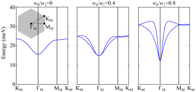
Figure 1: Exact charge $\pm 1$ excitations given by the simplified excitation matrix (Eq. 20) for three different $w_{0}/w_{1}$ at the twist angle $\theta=1.05^{\circ}$. Here we change $w_{0}$ while keeping $w_{1}=110\mathrm{meV}$ fixed. Other parameters are given in App. A. These excitations are exact at the charge neutrality point ($\nu=0$) for generic state and are exact at finite integer fillings if the flat metric condition is satisfied. The charge +1 and $-1$ excitations are degenerate. The exact charge $\pm 1$ excitations obtained using the full excitation matrix (Section III.1) without assuming the flat metric condition are given in Figs. 5 and 6 in Section C.4. The charge gap in those cases shrinks considerably.

To find the charge one excitations (adding an electron into the system), we sum the commutators in Section II over $\mathbf{q},\mathbf{G}$, and use the fact that the ground states in Eqs. 8 and 10 satisfy $(O_{\mathbf{q,G}}-A_{\mathbf{G}}N_{M}\delta_{\mathbf{q},0})|\Psi\rangle=0$ for coefficient $A_{\mathbf{G}}$ in Eq. (9) in their corresponding limits. For any state $|\Psi\rangle$ in Eqs. 8 and 10, we find:

$$\left[H_{I}-\mu N,c_{\mathbf{k},n,\eta,s}^{\dagger}\right]|\Psi\rangle=\frac{1}{2\Omega_{\text{tot}}}\sum_{m}R_{mn}^{\eta}(\mathbf{k})c_{\mathbf{k},m,\eta,s}^{\dagger}|\Psi\rangle\ ,$$ (18)

where $N$ is the electron number operator, and the matrix

$$R_{mn}^{\eta}(\mathbf{k})=\sum_{\mathbf{G}\mathbf{q}m^{\prime}}V(\mathbf{G}+\mathbf{q})M_{m^{\prime}m}^{\left(\eta\right)*}\left(\mathbf{k},\mathbf{q}+\mathbf{G}\right)M_{m^{\prime}n}^{\left(\eta\right)}\left(\mathbf{k},\mathbf{q}+\mathbf{G}\right)$$

$$\qquad+\sum_{\mathbf{G}}2N_{M}A_{-\mathbf{G}}\sqrt{V(\mathbf{G})}M_{m,n}^{\left(\eta\right)}\left(\mathbf{k},\mathbf{G}\right)-\mu\delta_{mn}.$$ (19)

We hence see that, if $|\Psi\rangle$ is one of the $|\Psi_{\nu}^{\nu_{+},\nu_{-}}\rangle$ Eq. (10) or one of the $|\Psi_{\nu}\rangle$ Eq. (8) eigenstates of $H_{I}$, then $c_{\mathbf{k},m,\eta,s}^{\dagger}|\Psi\rangle\$ can be recombined as eigenstates of $H_{I}$ with eigenvalues obtained by diagonalizing the $2\times 2$ matrix $R_{mn}^{\eta}(\mathbf{k})$.

In the nonchiral case, the eigenstates $|\Psi_{\nu}\rangle$ we found in Ref. Lian et al. (2020b) (and re-written in Eq. (8)) have both active bands $n=\pm 1$ in each valley $\eta$ and spin $s$ either fully occupied or fully empty.

In this case, we can consider two charge $+1$ states $c_{\mathbf{k},n,\eta,s}^{\dagger}|\Psi\rangle$ ($n=\pm$) at a fixed $\mathbf{k}$ in a fully empty valley $\eta$ and spin $s$. These two states then form a closed subspace with a $2\times 2$ subspace Hamiltonian $R^{\eta}(\mathbf{k})$ defined by Eq. (III.1). Diagonalizing the matrix $R^{\eta}(\mathbf{k})$ then gives the excitation eigenstates and excitation energies. Furthermore, at $\nu=0$, the state $|\Psi_{\nu=0}\rangle$ in Eq. (8) is the ground state of the interaction Hamiltonian $H_{I}$ regardless of the flat metric condition Eq. (11), and hence $c_{\mathbf{k},n,\eta,s}^{\dagger}|\Psi_{\nu=0}\rangle$ always gives the charge excitation above the ground state.

If we further assume the flat band condition Eq. (11) (or its violation is small enough), all eigenstates $|\Psi_{\nu}\rangle$ become exact ground states and the second row of Section III.1 vanishes (see Section C.1.1). Since the U(4) irrep of the ground state $|\Psi_{\nu}\rangle$ is $[(2N_{M})^{(\nu+4)/2}]_{4}$, the U(4) irrep of the charge 1 excited state is given by $[(2N_{M})^{(\nu+4)/2},1]_{4}$. A similar equation for the charge $-1$ excitations is derived in in Section C.3, where we denote the excitation matrix as $\widetilde{R}$.

As explained in Section A.3, when the flat metric condition is satisfied, the second term in $R^{\eta}$ (Section III.1) can be canceled by the chemical potential term (the third term), and thus we obtain a simplified expression for $R^{\eta}$ independent of $\nu$:

$$R_{mn}^{\eta}(\mathbf{k})= \sum_{\mathbf{G}\mathbf{q}m^{\prime}}V(\mathbf{G}+\mathbf{q})M_{m^{\prime}m}^{\left(\eta\right)*}\left(\mathbf{k},\mathbf{q}+\mathbf{G}\right)M_{m^{\prime}n}^{\left(\eta\right)}\left(\mathbf{k},\mathbf{q}+\mathbf{G}\right).$$ (20)

It is worth noting that Eq. 20 is exact for $\nu=0$ even without the flat metric condition Eq. (11), because the coefficient $A_{\mathbf{G}}$ (Eq. 9) in the second term of $R^{\eta}$ (Section III.1) and the chemical potential in the third term of $R^{\eta}$ vanish at $\nu=0$.

The simplified matrix $\widetilde{R}^{\eta}$ for charge $-1$ excitation with the flat metric condition Eq. (11) is the complex conjugation of $R^{\eta}$, i.e., $\widetilde{R}^{\eta}_{mn}(\mathbf{k})={R}^{\eta*}_{mn}(\mathbf{k})$. This shows that, the charge $-1$ excitations are degenerate with the charge $+1$ excitations if either $\nu=0$ or the flat metric condition Eq. (11) is satisfied.

The charge $+1$ excitation dispersion determined by Eq. 20 (which does not depend on $\nu$) is plotted in Fig. 1.

The parameters used in the calculation to obtain the spectrum are given in App. A. We find that, with the flat metric condition imposed, the charge $\pm 1$ excitation (Fig. 1) is gapped, and the minimum is at the $\Gamma$ point, with a large dispersion velocity. The exact charge $\pm 1$ excitations at different fillings obtained using the full $R^{\eta}$ matrix (Section III.1) of realistic parameters (which break the flat metric condition Eq. (11)) are given in Figs. 5 and 6 in Section C.4.

The degeneracy of the excitation spectrum depends on the filling $\nu$ of the ground state. In the nonchiral-flat U(4) limit, $R^{\eta}$ does not depend on spin, and $R^{+}$, $R^{-}$ have the same eigenvalues because they are related by the symmetry $C_{2z}P$, where $P$ is a single-body unitary PH symmetry (Section A.2.1) Song et al. (2019); Bernevig et al. (2020b); Song et al. (2020). Thus charge $+1$ excitations in different valley-spin flavors have the same energy. For the state $|\Psi_{\nu}\rangle$ (Eq. 8), the $+1$ excitations in the empty $(4-\nu)/2$ spin-valley flavors are degenerate. Correspondingly, $-1$ excitations in the occupied $(4+\nu)/2$ spin-valley flavors are also degenerate.

In the (first) chiral-flat limit, and with the flat metric condition Eq. (11) (or at $\nu=0$ without (11)), the expression for the charged excitations in the Chern basis $d^{\dagger}_{\mathbf{k},e_{Y},\eta,s}|\Psi_{\nu}^{\nu_{+},\nu_{-}}\rangle$ becomes diagonal and independent of $e_{Y}$ (see Section C.2 for the chiral-flat limit without the flat metric condition Eq. (11)):

$$\left[H_{I}-\mu N,d_{\mathbf{k},e_{Y},\eta,s}^{\dagger}\right]|\Psi\rangle= \frac{1}{2\Omega_{\text{tot}}}R_{0}(\mathbf{k})d_{\mathbf{k},e_{Y},\eta,s}^{\dagger}|\Psi\rangle,$$

$$R_{0}(\mathbf{k})= \sum_{\mathbf{G},\mathbf{q}}P(\mathbf{k},\mathbf{q}+\mathbf{G}),$$ (21)

provided that the Chern band $e_{Y}(=\pm 1)$ in valley $\eta$ and spin $s$ is fully empty and $P(\mathbf{k},\mathbf{q}+\mathbf{G})$ given in Section II. We obtain

$$R_{0}(\mathbf{k})=\sum_{\mathbf{G},\mathbf{q}}V(\mathbf{G}+\mathbf{q})[\alpha_{0}(\mathbf{k},\mathbf{q}+\mathbf{G})^{2}+\alpha_{2}(\mathbf{k},\mathbf{q}+\mathbf{G})^{2}].$$ (22)

The spectrum at the magic angle is shown in Fig. 1. The U(4)$\times$U(4) irrep of the charge +1 excited states with $e_{Y}=1$ and $e_{Y}=-1$ are given by $\left([N_{M}^{\nu_{+}},1]_{4},[N_{M}^{\nu_{-}}]_{4}\right)$ and $\left([N_{M}^{\nu_{+}}]_{4},[N_{M}^{\nu_{-}},1]_{4}\right)$, respectively. The charge $-1$ excitation details can be found in Section C.3.

Since in the chiral-flat limit the scattering matrix $R_{0}(\mathbf{k})$ is identity in the $e_{Y}$ space, the excitation has degeneracy in addition to the valley-spin degeneracies. For a state in Eq. 10 with filling $\nu$, the charge $+1$ and $-1$ excitations have degeneracies $4-\nu$ and $4+\nu$, respectively.

III.2 Bounds on the charge $\pm 1$ excitation gap

In this subsection, we will focus on the charge neutrality point ($\nu=0$), where the second and third terms in $R^{\eta}(\mathbf{k})$ (Section III.1) vanish, and nonzero integer fillings $\nu=\pm 1,\pm 2,\pm 3$ with the flat metric condition Eq. (11) such that the second and third terms in $R^{\eta}(\mathbf{k})$ cancel each other. In these cases $R^{\eta}(\mathbf{k})$ is a positive semidefinite matrix and hence has non-negative eigenvalues. We are able to obtain some analytical bounds for the gap of the $\pm 1$ excitation. Detail calculations are given in Section C.1.2. Since charge $\pm 1$ excitations in this case are degenerate, our conclusion below for charge +1 excitations also apply to charge -1 excitations.

We rewrite the $R^{\eta}(\mathbf{k})$ matrix as $R_{mn}^{\eta}(\mathbf{k})=(M^{\left(\eta\right)\dagger}(\mathbf{k})VM^{\left(\eta\right)}(\mathbf{k}))_{mn}$, where now $M^{\left(\eta\right)}(\mathbf{k})$ with given $\eta$ and $\mathbf{k}$ is a matrix of the dimension $2N_{M}\cdot N_{\mathbf{G}}\times 2$ (with $2$ because we are projecting into the two active TBG bands). $N_{M}$ is number of moiré unit cells, $N_{\mathbf{G}}$ is the number of plane waves (MBZs) taken into consideration. By separating the $\{\mathbf{q},\mathbf{G}\}=0$ contribution, and using Weyl’s inequalities we find in Section C.1.2 that the energies of the excited states are $\geq\frac{1}{2}V(\mathbf{q}=0)/\Omega_{\text{tot}}$. The bound $\frac{1}{2}V(\mathbf{q}=0)/\Omega_{\text{tot}}$ is small but nonzero for large but finite $\Omega_{\rm tot}$. This shows that the states $c_{\mathbf{k},n,\eta,s}^{\dagger}|\Psi\rangle$ are not exactly degenerate to the ground state $|\Psi\rangle$ (note that we did not prove these are the unique ground states).

The excited states of the PSDH appears to give rise to finite gap charge 1 excitations. The largest gap happens in the atomic limit or a material, where $\langle{u_{m}(\mathbf{k}+\mathbf{q})}|u_{n}(\mathbf{k})\rangle=\delta_{mn}$, for which $R_{mn}=\delta_{mn}\sum_{\mathbf{q},\mathbf{G}}V(\mathbf{q}+\mathbf{G})=\delta_{mn}\Omega_{\rm tot}V(\bf{r}=0)$. Hence the gap is $\frac{1}{2}V(\mathbf{r}=0)$. Away from the atomic limit, the gap is reduced, but will generically remain finite. We now give an argument for this. Since we know that TBG is far away from an atomic limit - the bands being topological, we expect a reduction in this gap. We perform a different decomposition of the matrix $R_{mn}^{\eta}$: we separate it into $\mathbf{G}=\mathbf{0}$ and $\mathbf{G}\neq 0$ sums (see Section C.1.3). The $\mathbf{G}\neq 0$ part, besides being negligible for $|\mathbf{G}|\geq\sqrt{3}k_{\theta}$ Bernevig et al. (2020a), is also positive semidefinite, and the eigenvalues of $R_{mn}^{\eta}$ are bounded by (and close to) the $\mathbf{G}=0$ part:

$$R_{mn}^{\eta}(\mathbf{k})\geq\sum_{\mathbf{q}}V(\mathbf{q})M_{m^{\prime},m}^{\left(\eta\right)*}\left(\mathbf{k},\mathbf{q}\right)M_{m^{\prime},n}^{\left(\eta\right)}\left(\mathbf{k},\mathbf{q}\right),$$ (23)

where $\mathbf{q}$ is summed over the MBZ, and the inequality means that the eigenvalues of the left hand side are equal to or larger than the eigenvalues of the right hand side. We then re-write the right hand side as $\sum_{\mathbf{q}}V(\mathbf{q})(\delta_{mn}-\mathfrak{G}_{\eta}^{mn}(\mathbf{k},\mathbf{q}))$, where we call the positive semi-definite matrix $\mathfrak{G}^{mn}(\mathbf{k},\mathbf{q})$ the generalized “quantum geometric”, whose trace is the generalized Fubini-Study metric. For small momentum transfer $\mathbf{q}$, we can show that $\mathfrak{G}^{mn}(\mathbf{k},\mathbf{q})=\sum_{ij}q_{i}q_{j}\mathfrak{G}^{mn}_{ij}(\mathbf{k})+\mathcal{O}(q^{3})$. where $\mathfrak{G}^{mn}_{ij}(\mathbf{k})$ is the conventional quantum geometric tensor (and the Fubini-Study metric) Xie et al. (2020a); Neupert et al. (2013) defined by

$$\mathfrak{G}^{mn}_{ij}(\mathbf{k}) =\sum_{a,b=1}^{N}\partial_{k_{i}}u^{*}_{a,m}(\mathbf{k})\bigg{(}\delta_{a,b}-\sum_{l\in\mathcal{B}}u_{a,l}(\mathbf{k})u^{*}_{b,l}(\mathbf{k})\bigg{)}$$

$$\times\partial_{k_{j}}u_{b,n}(\mathbf{k}),$$ (24)

in which $m,n\in\mathcal{B}$ are energy band indices and $i,j$ are spatial direction indices of the orthonormal vectors $u_{m}(\mathbf{k})$ in a $N$ dimensional Hilbert space, with $\mathbf{k}$ being the momentum (or other parameter). The $\mathfrak{G}^{mn}(\mathbf{k},\mathbf{q})$ tensor quantifies the distance between two eigenstates in momentum space.

Generically, we expect Xie et al. (2020a) that the inner product between two functions at $\mathbf{k}$ and $\mathbf{k}+\bf{q}$ to fall off as $\bf{q}$ increases, leaving a finite term in $R_{mn}^{\eta}(\mathbf{k})$, the electron gap, at every $\bf{k}$. In trivial bands in the atomic limit, the positive semi-definite matrix $\mathfrak{G}^{mn}(\mathbf{k},\mathbf{q})$ reaches its theoretical lower bound 0 and hence the charge 1 gap is maximal. In topological bands, such as TBG, the quantum metric has a lower bound and hence the charge 1 gap is reduced.

IV Charge neutral excitations

IV.1 Method to obtain charge neutral excitations

To obtain the charge neutral excitations, we choose the natural basis $c_{\mathbf{k}+\mathbf{p},m_{2},\eta_{2},s_{2}}^{\dagger}c_{\mathbf{k},m_{1},\eta_{1},s_{1}}|\Psi\rangle$, where $|\Psi\rangle$ is any of the exact ground states and/or eigenstates in Eqs. 10 and 8 and $\mathbf{p}$ is the momentum of the excited state. The scattering matrix of these basis can be solved as easily as a one-body problem, despite the fact that Eqs. 10 and 8 hold a thermodynamic number of electrons. The details are given in App. D. For $|\Psi\rangle$ being a state in Eq. 8, the scattering of $c_{\mathbf{k}+\mathbf{p},m_{2},\eta_{2},s_{2}}^{\dagger}c_{\mathbf{k},m_{1},\eta_{1},s_{1}}|\Psi\rangle$ by the interaction is:

$$\left[H_{I}-\mu N,c_{\mathbf{k}+\mathbf{p},m_{2},\eta_{2},s_{2}}^{\dagger}c_{\mathbf{k},m_{1},\eta_{1},s_{1}}\right]|\Psi_{\nu}\rangle$$

$$= \frac{1}{2\Omega_{\text{tot}}}\sum_{m,m^{\prime}}\sum_{\mathbf{q}}S^{(\eta_{2},\eta_{1})}_{m,m^{\prime};m_{2},m_{1}}(\mathbf{k}+\mathbf{q},\mathbf{k};\mathbf{p})$$

$$\qquad\times c_{\mathbf{k}+\mathbf{p}+\mathbf{q},m,\eta_{2},s_{2}}^{\dagger}c_{\mathbf{k}+\mathbf{q},m^{\prime},\eta_{1},s_{1}}|\Psi_{\nu}\rangle,$$ (25)

$$S^{(\eta_{2},\eta_{1})}_{m,m^{\prime};m_{2},m_{1}}(\mathbf{k}+\mathbf{q},\mathbf{k};\mathbf{p})$$ (26)

$$= \delta_{\mathbf{q},0}(\delta_{m,m_{2}}\widetilde{R}_{m^{\prime}m_{1}}^{\eta_{1}}(\mathbf{k})+\delta_{m^{\prime},m_{1}}R_{mm_{2}}^{\eta_{2}}(\mathbf{k}+\mathbf{p}))$$

$$- 2\sum_{\mathbf{G}}V(\mathbf{G}+\mathbf{q})M_{m,m_{2}}^{\left(\eta_{2}\right)}\left(\mathbf{k}+\mathbf{p},\mathbf{q}+\mathbf{G}\right)M_{m^{\prime},m_{1}}^{\left(\eta_{1}\right)*}\left(\mathbf{k},\mathbf{q}+\mathbf{G}\right),$$

where $R_{mn}^{\eta}(\mathbf{k})$ (Section III.1) and $\widetilde{R}_{mn}^{\eta}(\mathbf{k})$ are the charge $\pm 1$ excitation matrices. A valley-spin flavor in $|\Psi_{\nu}\rangle$ (Eq. 8) is either fully occupied or fully empty, thus $\{\eta_{1},s_{1}\}$ belongs to the valley-spin flavors which are fully occupied, while $\{\eta_{2},s_{2}\}$ belongs to the valley-spin flavors which are not occupied. Eq. 26 shows that the neutral excitation scattering matrix is a sum of the two single-particle energies ($\delta_{m,m_{2}}\widetilde{R}_{mm_{1}}^{\eta_{1}}(\mathbf{k}_{1})+\delta_{m,m_{1}}R_{mm_{2}}^{\eta_{2}}(\mathbf{k}_{2})$) plus an interaction term. By translation invariance, the scattering preserves the total momentum $\mathbf{p}$. The spectrum of the charge neutral excitations at each $\mathbf{p}$ is a diagonalization problem of a matrix of the dimension $4N_{M}\times 4N_{M}$, where the left and right indices are $(\mathbf{k}+\mathbf{q},m,m^{\prime})$ and $(\mathbf{k},m_{2},m_{2})$, respectively.

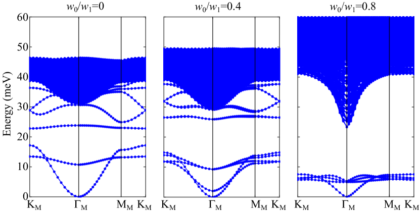
Figure 2: Exact charge neutral excitations with the flat metric condition being imposed for three different $w_{0}/w_{1}$ at the twist angle $\theta=1.05^{\circ}$. Here we change $w_{0}$ while keeping $w_{1}=110\mathrm{meV}$ fixed. Other parameters are given in App. A. These excitations are exact at the charge neutrality point ($\nu=0$) for generic states and are exact at finite integer fillings if the flat metric condition is satisfied. The exact charge neutral excitations at different fillings without imposing flat metric condition are given in Figs. 7 and 8 in Section D.4. Note the softening of further Goldstone modes from finite to zero $w_{0}$, reflecting the symmetry enhancement of the first chiral limit. The continuum above the Goldstone modes is fundamentally made of independent particle-hole excitations

The excitation spectrum with the flat metric condition Eq. (11) being imposed, i.e., with the $R^{\eta}$ (Section III.1) being replaced by the simplified Eq. 20, is shown in Fig. 2. As explained in Section III.1, the simplified charge $\pm 1$ matrices $R$ and $\widetilde{R}$ do not depend on the filling $\nu$. Thus the obtained charge neutral excitation dispersion also do not depend on $\nu$. Fig. 2 is exact for $\nu=0$ even when the flat metric condition is not satisfied since Eq. 20 is exact for $\nu=0$. The exact charge neutral excitations at different fillings without imposing the flat metric condition Eq. (11) are given in Figs. 7 and 8 in Section D.4.

It is worth noting that, in the Figs. 2, 7 and 8 we just plot the eigenvalues of the scattering matrix Eq. 26, which does not assume any information of the occupied valley-spin flavors in the ground state. In practice, for a given ground state $|\Psi\rangle$, the spectrum branch annihilating (creating) electrons in empty (occupied) states does not exist.

IV.2 Goldstone modes

Solving Eq. 26 provides us with the expression for the neutral excitations at momentum $\mathbf{p}$ on top of the TBG ground states, including the Goldstone mode, whose dispersion relation can be obtained in terms of the quantum geometry factors of the TBG. In general, the scattering matrix is not guaranteed to be positive semi-definite, and negative energy would imply instability of the ground states. However, in a large (physical) range of parameters (App. A) of TBG at the twist angle $\theta=1.05^{\circ}$, we find that, as shown in Figs. 2, 7 and 8, the energies of charge neutral excitations of the exact ground states $|\Psi_{\nu}\rangle$ in Eq. (8) in the nonchiral-flat limit and $|\Psi_{\nu}^{\nu_{+},\nu_{-}}\rangle$ in Eq. (10) in the chiral-flat limit are non-negative, implying these are indeed stable ground states. As shown in Figs. 5 and 7 and discussed in Sections C.4 and D.4, strong (first) chiral symmetry breaking may lead to an instability to a metallic phase.

Little group	Number of GMs	Ground states
U(4)$\times$U(4)	0	$|\Psi_{0}^{4,0}\rangle$
U(1)$\times$U(3)$\times$U(4)	3	$|\Psi_{-3}^{1,0}\rangle$, $|\Psi_{-1}^{3,0}\rangle$
U(2)$\times$U(2)$\times$U(4)	4	$|\Psi_{-2}^{2,0}\rangle$
U(1)$\times$U(3)$\times$U(1)$\times$U(3)	6	$|\Psi_{-2}^{1,1}\rangle$, $|\Psi_{0}^{3,1}\rangle$
U(2)$\times$U(2)$\times$U(1)$\times$U(3)	7	$|\Psi_{-1}^{2,1}\rangle$
U(2)$\times$U(2)$\times$U(2)$\times$U(2)	8	$|\Psi_{0}^{2,2}\rangle$

Table 1: The little groups (remaining symmetry subgroups) and the number of Goldstone modes (denoted by GMs in the table) of the ground states $|\Psi_{\nu}^{\nu_{+},\nu_{-}}\rangle$ in the (first) chiral-flat U(4)$\times$U(4) limit. Only $\nu\leq 0$ states are tabulated since the symmetry and Goldstone modes of $\nu>0$ states are same as the $\nu<0$ states since they are related by the many-body charge-conjugation operator (Section A.2.3) Bernevig et al. (2020b). Only states with $\nu_{+}\geq\nu_{-}$ are tabulated since $|\Psi_{\nu}^{\nu_{+},\nu_{-}}\rangle$ and $|\Psi_{\nu}^{\nu_{-},\nu_{+}}\rangle$ have the equivalent little groups upon interchanging of the two U(4)s, and thus have the same number of Goldstone modes.

Little group	Number of GMs	Ground states
U(1)$\times$U(3)	3	$|\Psi_{-2}\rangle$, $|\Psi_{2}\rangle$
U(2)$\times$U(2)	4	$|\Psi_{0}\rangle$

Table 2: The little groups (remaining symmetry subgroups) and the number of Goldstone modes (GMs) of the ground states $|\Psi_{\nu}\rangle$ in the nonchiral-flat U(4) limit.

In Tables 2 and 1 we have tabulated the little group (defined as the remaining symmetry subgroup of the state) and the number of Goldstone modes for each ground state in Eqs. 8 and 10. As examples, here we only derive the little groups and number of Goldstone modes for $|\Psi_{-2}^{1,1}\rangle$ (10) and $|\Psi_{-2}\rangle$ (8). The little groups and Goldstone modes for other states can be obtained by the same method. First we consider the ground state $|\Psi_{-2}^{1,1}\rangle$ in the (first) chiral-flat U(4)$\times$U(4) limit, which has vanishing total Chern number. Recall that the U(4)$\times$U(4) irrep of $|\Psi_{-2}^{1,1}\rangle$ is $([N_{M}^{1}]_{4},[N_{M}^{1}]_{4})$. In each of the $e_{Y}=\pm 1$ sectors, only one U(4) spin-valley flavor is occupied. Hence the little group of the state $|\Psi_{-2}^{1,1}\rangle$ in each $e_{Y}$ sector is U(1)$\times$U(3), where the U(1) is the phase rotation in the occupied flavor and the U(3) is the unitary rotations within the 3 empty flavors. Thus, the total little group of the state $|\Psi_{-2}^{1,1}\rangle$ is U(1)$\times$U(3)$\times$U(1)$\times$U(3), which has the rank (number of independent generators) 20. Since the Hamiltonian has a symmetry group U(4)$\times$U(4) which has rank $32$, we find the number of broken symmetry generators to be 32-20=12. On the other hand, since all the Goldstone modes we derived are quadratic (similar to the SU(2) ferromagnets, see Eq. (30)), it is known that Nielsen and Chadha (1976) the number of Goldstone modes is equal to $1/2$ of the number of broken generators, namely, $12/2=6$. This is because a quadratic Goldstone mode is always a complex boson, which is equivalent to two real boson degrees of freedom corresponding to 2 broken generators.

Next, we consider the ground state $|\Psi_{-2}\rangle$ in the nonchiral-flat U(4) limit. Since the U(4) irrep of $|\Psi_{-2}\rangle$ is $[2N_{M}]_{4}$, only one U(4) spin-valley flavor is occupied. Thus the little group of $|\Psi_{-2}\rangle$ is U(1)$\times$U(3), where the U(1) is within the occupied flavor and the U(3) is within the 3 empty flavors. Hence the number of broken generators is $16-10=6$, where 16 and 10 are the ranks of U(4)$\times$U(4) and U(1)$\times$U(3), and the number of (quadratic) Goldstone modes is 6/2=3.

In the above paragraph we have shown that state $|\Psi_{-2}^{1,1}\rangle$ in the chiral-flat limit has three more Goldstone modes than $|\Psi_{-2}\rangle$ in the nonchiral-flat limit, although their wavefunctions are identical. This is because, if we slightly go away from the (first) chiral-flat limit towards the nonchiral-flat limit, i.e., take the parameter $0<w_{0}\ll w_{1}$, some branches of the Goldstone modes will be gapped by a finite $w_{0}$, as shown in Figs. 2, 7 and 8.

The number of Goldstone modes can also be obtained by examining the scattering matrix in Eq. (26). Here we take $|\Psi_{-2}^{1,1}\rangle$ as an example. As discussed in Section IV.3, in the first chiral limit, the state $d^{\dagger}_{\mathbf{k+p},e_{Y2},\eta_{2},s_{2}}d_{\mathbf{k},e_{Y1},\eta_{1},s_{1}}|\Psi_{-2}^{1,1}\rangle$ will be scattered to $d^{\dagger}_{\mathbf{k^{\prime}+p},e_{Y2},\eta_{2},s_{2}}d_{\mathbf{k^{\prime}},e_{Y1},\eta_{1},s_{1}}|\Psi_{-2}^{1,1}\rangle$ through the scattering matrix $S_{e_{Y2},e_{Y1}}(\mathbf{k}^{\prime},\mathbf{k};\mathbf{p})$, which does not depend on $\eta_{1},s_{1},\eta_{2},s_{2}$, and $S_{e_{Y2},e_{Y1}}(\mathbf{k}^{\prime},\mathbf{k};\mathbf{0})$ has an exact zero state for $e_{Y2}=e_{Y1}$ (Section D.3). Now we count the number of Goldstone modes on top of $|\Psi_{-2}^{1,1}\rangle$ using this property of scattering matrix.

Suppose the occupied flavors in $|\Psi_{-2}^{1,1}\rangle$ are $\{e_{Y},\eta,s\}=\{+1,+,\uparrow\},\{-1,+,\uparrow\}$. Then, for the state $d^{\dagger}_{\mathbf{k+p},e_{Y1},\eta_{2},s_{2}}d_{\mathbf{k},e_{Y1},\eta_{1},s_{1}}|\Psi_{-2}^{1,1}\rangle$ to be non-vanishing, $\{e_{Y_{1}},\eta_{1},s_{1}\}$ can only take the values in the two $e_{Y}$-valley-spin flavors $\{+1,+,\uparrow\},\{-1,+,\uparrow\}$, and $\{\eta_{2},s_{2}\}$ can only take values in the other three valley-spin flavors in each $e_{Y}$ sector. There are in total 6 non-vanishing channels. Since each channel has an zero mode given by the zero of $S_{e_{Y1},e_{Y1}}(\mathbf{k}^{\prime},\mathbf{k};\mathbf{0})$, there are 6 Goldstone modes, consistent with the group theory analysis in Table 1.

IV.3 Exact Goldstone mode and its stiffness in the (first) chiral-flat U(4)$\times$U(4) limit

In the first chiral limit, we are able to obtain the Goldstone modes analytically. We pick the basis as $d^{\dagger}_{\mathbf{k+p},e_{Y2},\eta_{2},s_{2}}d_{\mathbf{k},e_{Y1},\eta_{1},s_{1}}|\Psi_{\nu}^{\nu_{+},\nu_{-}}\rangle$, where the valley-spin flavor $\{\eta_{1},s_{1}\}$ with Chern band basis $e_{Y1}$ is fully occupied and the valley-spin flavor $\{\eta_{2},s_{2}\}$ and Chern band basis $e_{Y2}$ is fully empty. The PSDH scatters the basis to

$$\sum_{\mathbf{k}^{\prime}}S_{e_{Y2},e_{Y1}}(\mathbf{k}^{\prime},\mathbf{k};\mathbf{p})d^{\dagger}_{\mathbf{k^{\prime}+p},e_{Y2},\eta_{2},s_{2}}d_{\mathbf{k^{\prime}},e_{Y1},\eta_{1},s_{1}}|\Psi_{\nu}^{\nu_{+},\nu_{-}}\rangle,$$ (27)

where the scattering matrix $S$ does not depend on $\eta_{1}$, $\eta_{2}$, $s_{1}$, $s_{2}$. The simple commutators between $O_{-\mathbf{q},-\mathbf{G}}O_{\mathbf{q},\mathbf{G}}$ and fermion creation and annihilation operators in the chiral limit (Section II) lead to a simple scattering matrix. We here focus on the $e_{Y1}=e_{Y2}$, $\mathbf{p}=0$ channel. For generic $\nu=0$ states and the $\nu=\pm 1,\pm 2,\pm 3$ states with flat metric condition (Eq. 11), we have

$$S_{e_{Y};e_{Y}}(\mathbf{k}+\mathbf{q},\mathbf{k};0)=$$

$$2\delta_{\mathbf{q},0}\sum_{\mathbf{G},\mathbf{q}^{\prime}}V(\mathbf{G}+\mathbf{q}^{\prime})[\alpha_{0}(\mathbf{k},\mathbf{q}^{\prime}+\mathbf{G})^{2}+\alpha_{2}(\mathbf{k},\mathbf{q}^{\prime}+\mathbf{G})^{2}]$$

$$-2\sum_{\mathbf{G}}V(\mathbf{G}+\mathbf{q})[\alpha_{0}(\mathbf{k,q+G})^{2}+\alpha_{2}(\mathbf{k,q+G})^{2}].$$ (28)

The general expression of $S_{e_{Y2};e_{Y1}}(\mathbf{k}+\mathbf{q},\mathbf{k};\mathbf{p})$ for all channels without imposing the flat metric condition is given in Section D.2. We first show the presence of an exact zero eigenstate of Section IV.3 by remarking that the scattering matrix $S_{e_{Y};e_{Y}}(\mathbf{k}+\mathbf{q},\mathbf{k};\mathbf{0})$ satisfies (irrespective of $\eta_{1,2},s_{1,2}$):

$$\sum_{\mathbf{q}}S_{e_{Y};e_{Y}}(\mathbf{k}+\mathbf{q},\mathbf{k};\mathbf{0})=0.$$ (29)

This guarantees that the rank of the scattering matrix is not maximal, and that there is at least one exact zero energy eigenstate, with equal amplitude on every state in the Hilbert space: $\sum_{\mathbf{k}}d^{\dagger}_{\mathbf{k},e_{Y},\eta_{2},s_{2}}d_{\mathbf{k},e_{Y},\eta_{1},s_{1}}|\Psi_{\nu}^{\nu_{+},\nu_{-}}\rangle$. More details are given in Sections D.3 and D.3.1. The U(4)$\times$ U(4) multiplet of this state is also at zero energy. Moreover, the scattering matrix $S_{e_{Y};e_{Y}}(\mathbf{k+q},\mathbf{k};\mathbf{0})$ is positive semi-definite. The details of this proof can be found in Section D.3.1.

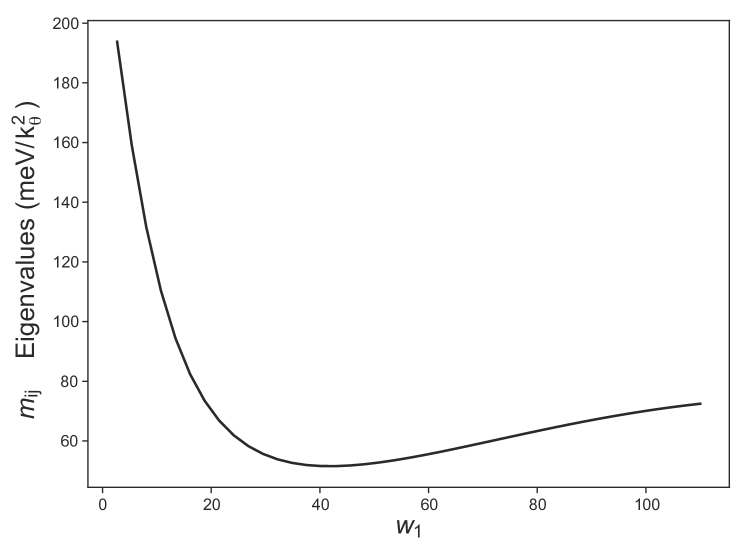
Figure 3: The eigenvalues of the mass tensor of the Goldstone mode in the first chiral limit (31). Here $w_{1}$ is in units of meV.

Since the $\mathbf{p}=\mathbf{0}$ state has zero energy, for small $\mathbf{p}$, by continuity, there will be low-energy states in the neutral continuum. By performing a k$\cdot$p perturbation in the $\mathbf{p}=0$ states in Eq. 115, one can compute the dispersion of the low-lying states. Full details are given in Section D.3.2. In the chiral limit, and imposing the flat metric condition Eq. 11 we find, by using $\alpha_{a}(\mathbf{k},\mathbf{q}+\mathbf{G})=\alpha_{a}(-\mathbf{k},-\mathbf{q}-\mathbf{G})$ for $a=0,2$ and as expected for the Goldstone of a FM, the linear term in $\mathbf{p}$ vanishes and

$$E_{\text{Goldstone}}(\mathbf{p})=\frac{1}{2}\sum_{ij=x,y}m_{ij}p_{i}p_{j}\ ,$$ (30)

to second order in $\mathbf{p}$. We find the Goldstone stiffness

$$m_{ij}=\frac{1}{2\Omega_{\text{tot}}}\sum_{\mathbf{k},\mathbf{q},\mathbf{G}}V(\mathbf{G}+\mathbf{q})\Big{[}\alpha_{0}(\mathbf{k},\mathbf{q}+\mathbf{G})\partial_{k_{i}}\partial_{k_{j}}\alpha_{0}(\mathbf{k},\mathbf{q}+\mathbf{G})+$$

$$\alpha_{2}(\mathbf{k},\mathbf{q}+\mathbf{G})\partial_{k_{i}}\partial_{k_{j}}\alpha_{2}(\mathbf{k},\mathbf{q}+\mathbf{G})+2\partial_{k_{i}}\alpha_{0}(\mathbf{k},\mathbf{q}+\mathbf{G})\partial_{k_{j}}\alpha_{0}(\mathbf{k},\mathbf{q}+\mathbf{G})$$

$$+2\partial_{k_{i}}\alpha_{2}(\mathbf{k},\mathbf{q}+\mathbf{G})\partial_{k_{j}}\alpha_{2}(\mathbf{k},\mathbf{q}+\mathbf{G})\Big{]}.$$ (31)

Since $C_{3z}$ symmetry is unbroken in the ground states in Eq. (10), an isotropic mass tensor $m_{ij}\propto\delta_{ij}$ is expected. The eigenvalues of $m_{ij}$ with different values of $w_{1}$ are plotted in Fig. 3.

V Charge $\pm 2$ excitations

V.1 Method to obtain $\pm 2$ excitations

We now derive the charge $\pm 2$ excitations. We choose a basis for the charge +2 excitations as $c_{\mathbf{k}+\mathbf{p},m_{2},\eta_{2},s_{2}}^{\dagger}c^{\dagger}_{-\mathbf{k},m_{1},\eta_{1},s_{1}}|\Psi\rangle$ where $|\Psi\rangle$ is any of the exact ground states and or eigenstates in Eqs. 8 and 10 (for which $(O_{\mathbf{q,G}}-A_{\mathbf{G}}N_{M}\delta_{\mathbf{q,0}})|\Psi\rangle=0$) and $\mathbf{p}$ is the momentum of the excited state. Hence $\{\eta_{1},s_{1}\}$, $\{\eta_{2},s_{2}\}$ belong to the valley-spin flavors which are not occupied. The details of the commutators of the Hamiltonian and the basis are given in App. E. We find

$$\left[H_{I}-\mu N,c_{\mathbf{k}+\mathbf{p},m_{2},\eta_{2},s_{2}}^{\dagger}c^{\dagger}_{-\mathbf{k},m_{1},\eta_{1},s_{1}}\right]|\Psi\rangle$$

$$= \frac{1}{2\Omega_{\text{tot}}}\sum_{m,m^{\prime},\mathbf{q}}T^{(\eta_{2},\eta_{1})}_{m,m^{\prime};m_{2},m_{1}}(\mathbf{k}+\mathbf{q},\mathbf{k};\mathbf{p})$$

$$\times c_{\mathbf{k}+\mathbf{q}+\mathbf{p},m,\eta_{2},s_{2}}^{\dagger}c^{\dagger}_{-\mathbf{k}-\mathbf{q},m^{\prime},\eta_{1},s_{1}}|\Psi\rangle,$$ (32)

$$T^{(\eta_{2},\eta_{1})}_{m,m^{\prime};m_{2},m_{1}}(\mathbf{k}+\mathbf{q},\mathbf{k};\mathbf{p})$$ (33)

$$= \delta_{\mathbf{q},0}(\delta_{m,m_{2}}R_{mm_{1}}^{\eta_{1}}(-\mathbf{k})+\delta_{m,m_{1}}R_{mm_{2}}^{\eta_{2}}(\mathbf{k+p}))$$

$$+ 2\sum_{\mathbf{G}}V(\mathbf{G}+\mathbf{q})M_{mm_{2}}^{\left(\eta_{2}\right)}\left(\mathbf{k}+\mathbf{p},\mathbf{q}+\mathbf{G}\right)M_{m^{\prime}m_{1}}^{\left(\eta_{1}\right)}\left(-\mathbf{k},-\mathbf{q}-\mathbf{G}\right),$$

where $R_{mn}^{\eta}(\mathbf{k})$ are the charge $+1$ excitation matrices in Section III.1. We see that the charge $+2$ excitation energy is a sum of the two single-particle energies plus an interaction energy. By the translational invariance, scattering preserves the momentum ($\mathbf{p}$) of the excited state. The spectrum of the excitations at a given $\mathbf{p}$ is a diagonalization problem of a matrix of the dimension $4N_{M}\times 4N_{M}$. The scattering matrix $\widetilde{T}$ of the charge $-2$ excitations is derived in Section E.4. It has the same form as $T$ here except that the charge $+1$ excitation matrix $R^{\eta}$ is replaced by charge $-1$ excitation matrix $\widetilde{R}^{\eta}$ and the $M$ matrix is replaced by the complex conjugation of $M$.

The spectrum of charge $\pm 2$ excitations with the flat metric condition Eq. (11) imposed is shown in Fig. 4. By imposing the flat metric condition, we can replace the $R^{\eta}$ matrix (Section III.1) in Eq. 33 by the simplified Eq. 20. Since Eq. 20 does not depend on $\nu$, the obtained charge $+2$ excitation dispersion also do not depend on $\nu$. Fig. 4 is exact for $\nu=0$ even when the flat metric condition is not satisfied since Eq. 20 is exact for $\nu=0$. Due to the many-body charge-conjugation symmetry at $\nu=0$ Bernevig et al. (2020b), the charge $-2$ excitations are degenerate with the charge $+2$ excitations. Exact charge $\pm 2$ excitations without imposing the flat metric condition Eq. (11) at different fillings are given in Figs. 9 and 10 in Section E.5.

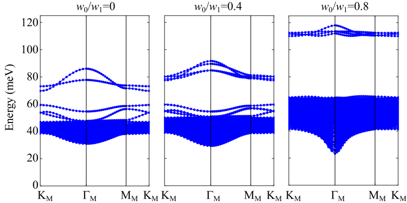
Figure 4: Exact charge $\pm 2$ excitations with the flat metric condition being imposed for three different $w_{0}/w_{1}$ at the twist angle $\theta=1.05^{\circ}$. Here we change $w_{0}$ while keeping $w_{1}=110\mathrm{meV}$ fixed. Other parameters are defined in App. A. These excitations are exact at charge neutrality point ($\nu=0$) for generic states and are exact at finite integer fillings if the flat metric condition is satisfied. The charge +2 and $-2$ excitations are degenerate. The exact charge $\pm 2$ excitations at different fillings without imposing the flat metric condition are given in Figs. 9 and 10 in Section E.5. Note bound states above but not below the two-particle continuum, confirming our analytic proof and showing the lack of Cooper pairing in TBG projected Coulomb Hamiltonians

V.2 Absence of Cooper pairing in the projected Coulomb Hamiltonian

The exact expression of the 2-particle excitation spectrum (Eq. 33) allows for the determination of the Cooper pair binding energy (if any). We notice the scattering matrix Eq. 33, $T^{(\eta_{2},\eta_{1})}(\mathbf{k}+\mathbf{q},\mathbf{k};\mathbf{p})$, differs by a sign from the neutral charge energy Eq. 26: It is the sum of energies of two charge $+1$ excitations at momenta $\mathbf{k}+\mathbf{p},-\mathbf{k}$ plus an interaction matrix, while Eq. 26 is the sum of charge $+1$ and $-1$ excitations minus an interaction matrix. This allows us to use the Richardson criterion Richardson (1963); Richardson and Sherman (1964); Richardson (1966, 1977) for the existence of Cooper pairing by examining the binding energy as follows:

$$\Delta(N+2)=E(N+2)+E(N)-2E(N+1)<0$$ (34)

where $E(N)$ is the energy of the lowest state at $N$-particles. We now assume that the lowest state of the charge $+2$ excitation continuum obtained by diagonalizing the matrices Eq. 33 is the lowest energy state at two particles above the ground state, which is confirmed by numerical calculations for a range of parameters Xie et al. (2020b). We note that Section III.1 is the charge $+1$ excitation. The lowest energy of the non-interacting $2$-particle spectrum is $2\min(R)$, where $\min(R)$ is the smallest eigenvalue of $R^{\eta}(\mathbf{k})$ over $\mathbf{k}\in$ MBZ and valley flavors $\eta=\pm$.

Hence we can write the binding energy as $\min(T)-2\min(R)$, where $\min(T)$ represents the minimal eigenvalues of $T^{(\eta_{2},\eta_{1})}(\mathbf{k}+\mathbf{q},\mathbf{k};\mathbf{p})$ over momenta $\mathbf{p}\in$ MBZ and different valley flavors $\eta_{2},\eta_{1}$. For later convenience, we denote the sum of the first two terms of Eq. 33 as

$$T^{(\eta_{2},\eta_{1})\prime}_{m,m^{\prime};m_{2},m_{1}}(\mathbf{k}+\mathbf{q},\mathbf{k};\mathbf{p})$$

$$= \delta_{\mathbf{q},0}(\delta_{m,m_{2}}R_{mm_{1}}^{\eta_{1}}(-\mathbf{k})+\delta_{m,m_{1}}R_{mm_{2}}^{\eta_{2}}(\mathbf{k+p}))$$ (35)

and the last term of Eq. 33 as

$$T^{(\eta_{2},\eta_{1}){\prime\prime}}_{m,m^{\prime};m_{2},m_{1}}(\mathbf{k}+\mathbf{q},\mathbf{k};\mathbf{p})=2\sum_{\mathbf{G}}V(\mathbf{G}+\mathbf{q})$$

$$\quad\times M_{mm_{2}}^{\left(\eta_{2}\right)}\left(\mathbf{k}+\mathbf{p},\mathbf{q}+\mathbf{G}\right)M_{m^{\prime}m_{1}}^{\left(-\eta_{1}\right)*}\left(\mathbf{k},\mathbf{q}+\mathbf{G}\right).$$ (36)

We therefore have $T=T^{\prime}+T^{\prime\prime}$ in short notations. Here we have used the time-reversal symmetry: $M^{(\eta_{1})}_{m^{\prime}m_{1}}(-\mathbf{k},-\mathbf{q}-\mathbf{G})=M^{(-\eta_{1})*}_{m^{\prime}m_{1}}(\mathbf{k},\mathbf{q}+\mathbf{G})$, as explained in Section E.3. We use Weyl’s inequalities to find sufficient conditions for the presence and absence of superconductivity. In particular, for given $\mathbf{p},\eta_{2},\eta_{1}$, the smallest eigenvalue of $T^{(\eta_{2},\eta_{1})}(\mathbf{k}+\mathbf{q},\mathbf{k};\mathbf{p})$ is smaller than the smallest eigenvalue of $T^{(\eta_{2},\eta_{1})\prime}(\mathbf{k}+\mathbf{q},\mathbf{k};\mathbf{p})$ plus the largest eigenvalue of $T^{(\eta_{2},\eta_{1}){\prime\prime}}(\mathbf{k}+\mathbf{q},\mathbf{k};\mathbf{p})$. Hence we have $\min(T)\leq\min(T^{\prime})+\max(T^{\prime\prime})=2\min(R)+\max(T^{\prime\prime})$.

Therefore, a sufficient criterion for the presence of Cooper pairing binding energy is that $T^{(\eta_{2},\eta_{1}){\prime\prime}}(\mathbf{k}+\mathbf{q},\mathbf{k};\mathbf{p})$ has all eigenvalues negative:

$$\forall\eta_{1},\eta_{2},\mathbf{p},\quad\text{Eig}[T^{(\eta_{2},\eta_{1})\prime\prime}_{mm^{\prime};m_{2}m_{1}}(\mathbf{k}+\mathbf{q},\mathbf{k};\mathbf{p})]<0.$$ (37)

On the other hand, for given $\mathbf{p},\eta_{2},\eta_{1}$, the smallest eigenvalue of $T^{(\eta_{2},\eta_{1})}(\mathbf{k}+\mathbf{q},\mathbf{k};\mathbf{p})$ is larger than the the smallest eigenvalue of $T^{(\eta_{2},\eta_{1})\prime}(\mathbf{k}+\mathbf{q},\mathbf{k};\mathbf{p})$ plus the smallest eigenvalue of $T^{(\eta_{2},\eta_{1}){\prime\prime}}(\mathbf{k}+\mathbf{q},\mathbf{k};\mathbf{p})$. Hence we have $\min(T)\geq\min(T^{\prime})+\min(T^{\prime\prime})=2\min(R)+\min(T^{\prime\prime})$. Therefore, a sufficient criterion for the absence of Cooper pairing binding energy is that $T^{(\eta_{2},\eta_{1}){\prime\prime}}(\mathbf{k}+\mathbf{q},\mathbf{k};\mathbf{p})$ is positive semi-definite:

$$\forall\eta_{1},\eta_{2},\mathbf{p},\quad\text{Eig}[T^{(\eta_{2},\eta_{1})\prime\prime}_{mm^{\prime};m_{2}m_{1}}(\mathbf{k}+\mathbf{q},\mathbf{k};\mathbf{p})]\geq 0.$$ (38)

From the charge $+2$ excitation spectra in Figs. 4, 9 and 10 we can see that the the spectrum of $T$ consists of two parts: the two-particle continuum, which is given by the sums of two charge $+1$ excitations, and a set of charge $+2$ collective modes above the the two-particle continuum. Thus it seems that $T^{\prime\prime}$ are always non-negative positive.

In Section E.3 we proved that, for the projected Coulomb Hamiltonian with the time-reversal symmetry, the matrix $T^{(\eta,-\eta){\prime\prime}}(\mathbf{k}+\mathbf{q},\mathbf{k};\mathbf{p})$, which corresponds to excitations of two particles from different valley, is positive semi-definite. Thus there is no inter-valley pairing superconductivity of the PSDH $H_{I}$ at the integer fillings $\nu$ of the ground states in Eqs. 8 and 10. We expect this property to hold slightly away from integer fillings. Since TBG shows superconductivity at $\nu=2$ or slightly away from integer fillings, our results show that either kinetic energy or phonons are responsible for pairing.

Here we briefly sketch the proof. We consider the expectation value of $T^{(\eta,-\eta){\prime\prime}}(\mathbf{k}+\mathbf{q},\mathbf{k};\mathbf{p})$ on an arbitrary complex function $\phi_{m_{2},m_{1}}(\mathbf{k})$:

$$\langle T^{\prime\prime}\rangle^{\eta}_{\phi}(\mathbf{p})= \sum_{\mathbf{k}_{1},\mathbf{k}_{2}}\sum_{mm^{\prime}m_{2}m_{2}}T^{(\eta,-\eta){\prime\prime}}(\mathbf{k}_{2},\mathbf{k}_{1};\mathbf{p})$$

$$\times\phi^{*}_{mm^{\prime}}(\mathbf{k}_{2})\phi_{m_{2},m_{1}}(\mathbf{k}_{1}).$$ (39)

As detailed in Section E.3, substituting the definition of the $M$ matrix (Eq. 4) into Section V.2, we can rewrite the expectation value as

$$\langle T^{\prime\prime}\rangle^{\eta}_{\phi}(\mathbf{p})= \frac{2}{N_{\mathbf{G}}}\sum_{\mathbf{k}_{1}\mathbf{k}_{2}\mathbf{G}_{1}\mathbf{G}_{2}}\mathrm{Tr}[W^{\dagger}(\mathbf{k}_{2}+\mathbf{G}_{2})W(\mathbf{k}_{1}+\mathbf{G}_{1})]$$

$$\times V(\mathbf{k}_{2}+\mathbf{G}_{2}-\mathbf{k}_{1}-\mathbf{G}_{1}),$$ (40)

where

$$W(\mathbf{k}+\mathbf{G})=\sum_{m_{2},m_{1},\mathbf{G}}u_{m_{2},\eta}(\mathbf{k}+\mathbf{p}+\mathbf{G})\phi_{m_{2},m_{1}}(\mathbf{k})u_{m_{1},\eta}^{\dagger}(\mathbf{k}+\mathbf{G}).$$ (41)

Here $u_{m_{2},\eta}(\mathbf{k}+\mathbf{G})$ is the $2N_{\mathbf{Q}}\times 1$ vector $u_{\mathbf{Q}-\mathbf{G},\alpha;m_{2},\eta}(\mathbf{k})$ and $W(\mathbf{k}+\mathbf{G})$ is a $2N_{\mathbf{Q}}\times 2N_{\mathbf{Q}}$ matrix, with $N_{\mathbf{Q}}$ being the $\mathbf{Q}$ lattice size (see App. A.1 for definition of the $\mathbf{Q}$ lattice). For simplicity, we use $a$ and $b$ to represent the composite indices $(\mathbf{Q},\alpha)$. Then $\langle T^{\prime\prime}\rangle^{\eta}_{\phi}(\mathbf{p})$ can be written as $\sum_{ab}W_{ab}^{\dagger}VW_{ab}$, where now $W_{ab}$ is viewed as an $N_{M}\times 1$ vector and $V$ an $N_{M}\times N_{M}$ matrix. Since $V$ is positive semi-definite, for each pair of $a,b$, the summation over $\mathbf{k}_{1},\mathbf{k}_{2},\mathbf{G}_{1},\mathbf{G}_{2}$ is non-negative. Thus $T^{\prime\prime}$ is positive semi-definite since $\langle T^{\prime\prime}\rangle^{\eta}_{\phi}(\mathbf{p})\geq 0$ for arbitrary $\phi$.

In Section E.3 we also proved that, for $\eta_{2}=\eta_{1}=\eta$, $T^{(\eta,\eta){\prime\prime}}(\mathbf{k}+\mathbf{q},\mathbf{k};\mathbf{p})$ is also positive semi-definite due to the symmetry $PC_{2z}T$, with $P$ being the unitary single-body PH symmetry of TBG Song et al. (2019, 2020). Therefore, neither the inter-valley pairing nor the intra-valley Cooper pair has binding energy in the projected Coulomb Hamiltonian for any integer fillings $\nu$ in the chiral-flat limit, and for any even fillings $\nu=0,\pm 2,\pm 4$ in the nonchiral-flat limit.

VI Conclusions

In this paper, we have calculated the excitation spectra of a series positive semi-definite Hamiltonians (PSDHs) initially introduced by Kang and Vafek Kang and Vafek (2019) that generically appear Bernevig et al. (2020b) in projected Coulomb Hamiltonians to bands with nonzero Berry phases and which exhibit ferromagnetic states as ground states, under weak assumptions Lian et al. (2020b); Bernevig et al. (2020b) . These assumptions were also used by Kang and Vafek Kang and Vafek (2019) to find the $\nu=2$ ground states in TBG. In this paper, we show that not only the ground states, but a large number of low-energy excited states can be obtained in PSDHs. We obtain the general theory for the charge $\pm 1,\pm 2$ and neutral excitations energies and eigenstates and particularize it to the case of TBG insulating states. We find that charge $+1$ excitations are gapped, with the smallest gap at the $\Gamma$ point. In both the (first) chiral-flat limit and the nonchiral-flat limit, we find the Goldstone stiffness of the ferromagnetic state, as well as the Cooper pairing binding at integer fillings. In particular, we proved by the Richardson criterion Richardson (1963); Richardson and Sherman (1964); Richardson (1966, 1977) that Cooper pairing is not favored at integer fillings (even fillings when nonchiral) in the flat band limit. Since superconductivity has been observed in experiments with screened Coulomb potentials Stepanov et al. (2020); Saito et al. (2020a); Liu et al. (2020a) (such as at $\nu=2$), we conjecture the origin of superconductivity in TBG is not Coulomb, but is contributed by other mechanisms, e.g., the electron-phonon interaction Lian et al. (2019); Wu et al. (2018); Lewandowski et al. (2020), or due to kinetic terms. In particular, our theorem shows that the Luttinger-Kohn mechanism of creating attractive interactions out of repulsive Coulomb forces is ineffective for flat bands. A similar statement can be made for the super-exchange interaction. A finite kinetic energy is hence required for these mechanisms.

In future work, the charge excitation energies of these Hamiltonians will be obtained in perturbation theory with the kinetic terms. A further question, of whether there are other further eigenstates of the PSDHs, remains unsolved.

B.A.B thanks Oskar Vafek for fruitful discussions, and for sharing their similar results on this problem before publication Vafek and Kang (2020), where they also compute the Goldstone and charge 1 excitation spectrum, which agrees with ours. B.A.B also thanks Pablo Jarillo-Herrero for discussions and for pointing out Ref. Park et al. (2020). This work was supported by the DOE Grant No. DE-SC0016239, the Schmidt Fund for Innovative Research, Simons Investigator Grant No. 404513, the Packard Foundation, the Gordon and Betty Moore Foundation through Grant No. GBMF8685 towards the Princeton theory program, and a Guggenheim Fellowship from the John Simon Guggenheim Memorial Foundation. Further support was provided by the NSF-EAGER No. DMR 1643312, NSF-MRSEC No. DMR-1420541 and DMR-2011750, ONR No. N00014-20-1-2303, Gordon and Betty Moore Foundation through Grant GBMF8685 towards the Princeton theory program, BSF Israel US foundation No. 2018226, and the Princeton Global Network Funds. B.L. acknowledge the support of Princeton Center for Theoretical Science at Princeton University during the early stage of this work.

Appendix A Review of notation: single particle and interacting Hamiltonians

For completeness, we here briefly review the notations used for the single-particle and interacting Hamiltonians. Their properties and (explicit and hidden) symmetries of both the single particle and the interacting problems are detailed at length in our recent papers Bernevig et al. (2020a); Song et al. (2020); Bernevig et al. (2020b); Lian et al. (2020b).

A.1 Single particle Hamiltonian: short review of notation

The single-particle Hamiltonian, symmetries, and properties of the wavefunctions have been discussed at length in Ref. Bernevig et al. (2020a); Song et al. (2020, 2019). For completeness of notation, we give its expression here, for completeness, but we skip all details. The total single particle Hamiltonian is

$$\hat{H}_{0}=\sum_{\mathbf{k}\in\mathrm{MBZ}}\sum_{\eta\alpha\beta s}\sum_{\mathbf{Q}\mathbf{Q}^{\prime}}\Big{[}h_{\mathbf{Q}\mathbf{Q}^{\prime}}^{\left(\eta\right)}\left(\mathbf{k}\right)\Big{]}_{\alpha\beta}c_{\mathbf{k},\mathbf{Q},\eta,\alpha s}^{\dagger}c_{\mathbf{k},\mathbf{Q}^{\prime},\eta,\beta s}.$$ (42)

where $c_{\mathbf{k},\mathbf{Q},\eta,\alpha s}^{\dagger}$ is the creation operator at momentum $\mathbf{k}$ (in the moiré BZ - MBZ) in valley $\eta$ ($\pm$), sublattice $\alpha$ (1,2), spin $s$ ($\uparrow\downarrow$), and moiré momentum lattice $\mathbf{Q}$. The Hamiltonians in the two valleys are

$$h_{\mathbf{Q}\mathbf{Q}^{\prime}}^{\left(+\right)}\left(\mathbf{k}\right)=\delta_{\mathbf{Q},\mathbf{Q}^{\prime}}v_{F}\left(\mathbf{k}-\mathbf{Q}\right)\cdot\boldsymbol{\sigma}+\sum_{j=1}^{3}\left(\delta_{\mathbf{Q}-\mathbf{Q}^{\prime},\mathbf{q}_{j}}+\delta_{\mathbf{Q}^{\prime}-\mathbf{Q},\mathbf{q}_{j}}\right)T_{j}$$

$$h_{\mathbf{Q}\mathbf{Q}^{\prime}}^{\left(-\right)}\left(\mathbf{k}\right)=\delta_{\mathbf{Q},\mathbf{Q}^{\prime}}v_{F}\left(\mathbf{k}-\mathbf{Q}\right)\cdot\boldsymbol{\sigma}^{*}+\sum_{j=1}^{3}\left(\delta_{\mathbf{Q}-\mathbf{Q}^{\prime},\mathbf{q}_{j}}+\delta_{\mathbf{Q}^{\prime}-\mathbf{Q},\mathbf{q}_{j}}\right)\sigma_{x}T_{j}\sigma_{x},$$ (43)

where $\boldsymbol{\sigma}=(\sigma_{x},\sigma_{y})$, $\boldsymbol{\sigma}^{*}=(-\sigma_{x},\sigma_{y})$ are Pauli matrices, $\small T_{j}=w_{0}\sigma_{0}+w_{1}(\cos\frac{2\pi}{3}(j-1)\sigma_{x}+\sin\frac{2\pi}{3}(j-1)\sigma_{y})$, and $\mathbf{q}_{j}=k_{\theta}C_{3z}^{j-1}(0,1)^{T}$ ($j=1,2,3$) with $k_{\theta}=2|K|\sin\frac{\theta}{2}$ being the distance of the Graphene $K$ momenta from the top layer and bottom layer, $\theta$ the twist angle, $w_{0}$ the interlayer AA-hopping, and $w_{1}$ the interlayer AB-hopping. $\mathbf{Q}$ belongs to a hexagonal momentum space lattice, $\mathbf{Q}\in\mathcal{Q}_{\pm}$, where $\mathcal{Q}_{\pm}=\mathcal{Q}_{0}\pm\mathbf{q}_{1}$. The eigenstates of Eq. 42 take the form

$$c_{\mathbf{k}n\eta s}^{\dagger}=\sum_{\mathbf{Q}\alpha}u_{\mathbf{Q}\alpha;n\eta}\left(\mathbf{k}\right)c_{\mathbf{k},\mathbf{Q},\eta,\alpha s}^{\dagger}.$$ (44)

where $c_{\mathbf{k}+\mathbf{G},\mathbf{Q},\eta\alpha s}^{\dagger}=c_{\mathbf{k},\mathbf{Q}-\mathbf{G},\eta\alpha s}^{\dagger}$, for any moiré reciprocal wavevector $\mathbf{G}$, and hence

$$u_{\mathbf{Q}\alpha;n\eta}\left(\mathbf{k}+\mathbf{G}\right)=u_{\mathbf{Q}-\mathbf{G},\alpha;n\eta}\left(\mathbf{k}\right)$$ (45)

such that $c_{\mathbf{k}+\mathbf{G},n\eta s}^{\dagger}=c_{\mathbf{k}n\eta s}^{\dagger}$. This is the MBZ periodic gauge.

In the numerical calculations, we take the parameters $\theta=1.05^{\circ}$, $|K|=1.703\mathrm{\mathring{A}}^{-1}$, $v_{F}=5.944{\rm eV\cdot\mathring{A}}$, $w_{1}=110$meV.

The projected kinetic Hamiltonian in the flat bands will be denoted by $H_{0}$ (without hat), which is given in Eq. (1).

A.2 Interaction Hamiltonian: short review of notation

The many-body Hamiltonian, symmetries, and properties of the wavefunctions, as well as the derivations, have been discussed at length in Refs. Bernevig et al. (2020b); Lian et al. (2020b). For completeness of notation, we give its expression here, for completeness, but we skip all details. The Hamiltonian before projection was derived to be (denoted by a hat) Bernevig et al. (2020b); Lian et al. (2020b):

$$\hat{H}_{I}=\frac{1}{2\Omega_{\mathrm{tot}}}\sum_{\mathbf{G}}\sum_{\mathbf{q}\in\mathrm{MBZ}}V\left(\mathbf{G}+\mathbf{q}\right)\delta\rho_{-\mathbf{G}-\mathbf{q}}\delta\rho_{\mathbf{G}+\mathbf{q}};\;\;\;\;V\left(\mathbf{r}\right)=\frac{1}{\Omega_{\mathrm{tot}}}\sum_{\mathbf{G}}\sum_{\mathbf{q}\in\mathrm{MBZ}}e^{-i\left(\mathbf{q}+\mathbf{G}\right)\cdot\mathbf{r}}V\left(\mathbf{q}+\mathbf{G}\right)$$ (46)

where

$$\delta\rho_{\mathbf{q+G}}=\sum_{\eta,\alpha,s,\mathbf{k},\mathbf{Q}}(c_{\mathbf{k+q},\mathbf{Q-G},\eta,\alpha,s}^{\dagger}c_{\mathbf{k},\mathbf{Q},\eta,\alpha,s}-\frac{1}{2}\delta_{\mathbf{q,0}}\delta_{\mathbf{G,0}})$$ (47)

is the total electron density at momentum $\mathbf{q+G}$ relative to the charge neutral point. $\Omega_{\mathrm{tot}}$ is the total area of the moiré lattice, $\mathbf{G}$ sums over moiré reciprocal lattice, and $\mathbf{q}$ sums over momenta in MBZ zone.

For the analytic derivations in the current paper, we keep $V(\mathbf{r})$ generic. For the numerical plots of the energy dispersion and other properties, we use twisted bilayer graphene Coulomb interactions screened by the electrons in the two planar conducting gates Throckmorton and Vafek (2012); Kang and Vafek (2019): $V\left(\mathbf{r}\right)=U_{\xi}\sum_{n=-\infty}^{\infty}\left(-1\right)^{n}/{\sqrt{\left(\mathbf{r}/\xi\right)^{2}+n^{2}}}$ with $\xi=10\mathrm{nm}$ being the distance between the two gates, $U_{\xi}=e^{2}/\left(\epsilon\xi\right)=26\mathrm{meV}$ (in Gauss units), $\epsilon\approx 6$ the dielectric constant of boron nitride. The derivation of this interaction was explained at length in Ref. Bernevig et al. (2020b); Lian et al. (2020b). It was also showed that the interaction has non-vanishing Fourier component only for intra-valley scattering to give

$$V\left(\mathbf{q}\right)=\left(\pi\xi^{2}U_{\xi}\right)\frac{\tanh\left(\xi q/2\right)}{\xi q/2}.$$ (48)

For the given values of the parameters, $V\left(\mathbf{q}\right)$ was plotted in Ref. Song et al. (2020) and is a slowly decreasing function of $|\mathbf{q}|$ in the BZ, reaching (around the magic angle) about half of its maximal value as $|\mathbf{q}|$ spans the whole MBZ around.

A.2.1 Gauge fixing and the projected interaction

We define for our many-body Hamiltonian the form-factors, also called the overlap matrix of a set of bands $m,n$ as

$$M_{m,n}^{\left(\eta\right)}\left(\mathbf{k},\mathbf{q}+\mathbf{G}\right)=\sum_{\alpha}\sum_{\mathbf{Q}}u_{\mathbf{Q}-\mathbf{G},\alpha;m\eta}^{*}\left(\mathbf{k}+\mathbf{q}\right)u_{\mathbf{Q},\alpha;n\eta}\left(\mathbf{k}\right),$$ (49)

In terms of which the projected density operator interaction and Hamiltonian to a set of bands denoted by $m,n$ can be written as

$$\begin{split}&H_{I}=\frac{1}{2\Omega_{\mathrm{tot}}}\sum_{\mathbf{G}}\sum_{\mathbf{q}\in\mathrm{MBZ}}V\left(\mathbf{G}+\mathbf{q}\right)\overline{\delta\rho}_{-\mathbf{G}-\mathbf{q}}\overline{\delta\rho}_{\mathbf{G}+\mathbf{q}}\\ &\overline{\delta\rho}_{\mathbf{G}+\mathbf{q}}=\sum_{\eta s}\sum_{mn\in\mathrm{proj}}\sum_{\mathbf{k}}M_{m,n}^{\eta}(\mathbf{k},\mathbf{q}+\mathbf{G})\left(c^{\dagger}_{\mathbf{k}+\mathbf{q},m,\eta,s}c_{\mathbf{k},n,\eta,s}-\frac{1}{2}\delta_{\mathbf{q},0}\delta_{mn}\right).\end{split}$$

For our working convenience, we then define the operator

$$O_{\mathbf{q},\mathbf{G}}=\sqrt{V(\mathbf{q}+\mathbf{G})}\overline{\delta\rho}_{\mathbf{G}+\mathbf{q}}.$$ (50)

This allows us to rewrite the projected interaction Hamiltonian $H_{I}$ into the form of Eqs. (2) and (3). While most of the projected Hamiltonian properties are valid for any number of projected bands that respect the symmetries of the system (including PH), in TBG at the first magic angle we usually are interested in the projection of the Hamiltonian onto the lowest two flat bands per spin per valley of TBG (8 bands in total). An important step in any calculations - especially numerical - is the gauge-fixing procedure. Different gauges for the wavefunctions, that make different symmetries of the form factors Eq. 49 more explicit, can be chosen. This is explained at length in our manuscript Ref. Bernevig et al. (2020b), but for completeness we briefly mention them here. We consider only $2$ active bands, the general gauge-fixing mechanism for projection in more than $2$ bands is found in Ref. Bernevig et al. (2020b). To fix the gauge of the Bloch wavefunctions in Eq. (44), $|\psi_{\mathbf{k},n,\eta,s}\rangle=\sum_{\mathbf{Q},\alpha}u_{\mathbf{Q},\alpha;m\eta}(\mathbf{k})c_{\mathbf{k},\mathbf{Q},\eta,\alpha,s}^{\dagger}|0\rangle$, where $u_{\mathbf{Q},\alpha;m\eta}(\mathbf{k})$ is the solution of the single-particle Hamiltonian $h_{\mathbf{Q}\mathbf{Q}^{\prime}}^{(\eta)}(\mathbf{k})$, in each $\eta=\pm$, $s=\uparrow\downarrow$ sector, we label the higher energy band by $m=+$ and the lower band by $m=-$. Due to the spin-SU(2) symmetry, we set the real space wavefunctions for $s=\uparrow\downarrow$ to be identical and omit the index $s$ for the single-particle states. For a symmetry operation $g$, the sewing matrices $B^{g}_{n^{\prime}\eta^{\prime},n\eta}(\mathbf{k})=\langle\psi_{g\mathbf{k},n^{\prime},\eta^{\prime}}|g|\psi_{\mathbf{k},n,\eta}\rangle$, which relate states at momentum $\mathbf{k}$ with states at the transformed momentum $g\mathbf{k}$ can be consistently chosen to be

$$B^{C_{2z}T}(\mathbf{k})=\zeta^{0}\tau^{0},\qquad B^{C_{2z}}(\mathbf{k})=\zeta^{0}\tau^{x},\qquad B^{P}(\mathbf{k})=i\zeta^{y}\tau^{z},\qquad B^{C_{2z}P}(\mathbf{k})=\zeta^{y}\tau^{y}$$ (51)

for the $C_{2z}T$, $C_{2z}$, $P$ symmetries of TBG where $\zeta^{a},\tau^{a}$ ($a=0,x,y,z$) are Pauli-matrices acting on the band and valley indices, respectively Bernevig et al. (2020b). Here $P$ is a unitary single-body PH symmetry that transforms $\mathbf{k}$ to $-\mathbf{k}$ Song et al. (2019, 2020). We leave the other sewing matrices - for $C_{3z}$, $C_{2x}$ - unfixed. With these sewing matrices, once we obtain, by diagonalizing the single particle Hamiltonian, the wavefunctions in the valley $\eta=+$ for band $m=+$, then we first fix the $C_{2z}T$ (in TBG, this is done at the detriment of the wavefunction being continuous), then we use of the PH to generate the $m=-$ band, while finally, using $C_{2z}$ symmetry to generate the wavefunctions in the valley $\eta=-$. In Ref. Bernevig et al. (2020b), we use the above gauge to determine the most generic form of the $M$ matrix coefficient (Eq. 49). We found that - away from the point $w_{1}=0$ in parameter space which we call “second chiral limit” - we can decompose the $M$ matrix into four terms: Song et al. (2020); Bernevig et al. (2020b)

$$M(\mathbf{k},\mathbf{q}+\mathbf{G})=\zeta^{0}\tau^{0}\alpha_{0}(\mathbf{k},\mathbf{q}+\mathbf{G})+\zeta^{x}\tau^{z}\alpha_{1}(\mathbf{k},\mathbf{q}+\mathbf{G})+i\zeta^{y}\tau^{0}\alpha_{2}(\mathbf{k},\mathbf{q}+\mathbf{G})+\zeta^{z}\tau^{z}\alpha_{3}(\mathbf{k},\mathbf{q}+\mathbf{G}).$$ (52)

where $\alpha_{0,1,2,3}$ are real functions which satisfy the following symmetry conditions.

$$\quad\alpha_{a}(\mathbf{k},\mathbf{q}+\mathbf{G})=\alpha_{a}(\mathbf{k}+\mathbf{q},-\mathbf{q}-\mathbf{G})\quad\text{for }a=0,1,3,\qquad\alpha_{2}(\mathbf{k},\mathbf{q}+\mathbf{G})=-\alpha_{2}(\mathbf{k}+\mathbf{q},-\mathbf{q}-\mathbf{G}),$$ (53)

$$\quad\alpha_{a}(\mathbf{k},\mathbf{q}+\mathbf{G})=\alpha_{a}(-\mathbf{k},-\mathbf{q}-\mathbf{G})\quad\text{for }a=0,2,\qquad\alpha_{a}(\mathbf{k},\mathbf{q}+\mathbf{G})=-\alpha_{a}(-\mathbf{k},-\mathbf{q}-\mathbf{G})\quad\text{for }a=1,3.$$ (54)

In particular, the combination of Eqs. (53) and (54) implies that at $\mathbf{q}=\mathbf{0}$, we have

$$\alpha_{0}(\mathbf{k},\mathbf{G})=\alpha_{0}(-\mathbf{k},\mathbf{G})\ ,\qquad\alpha_{j}(\mathbf{k},\mathbf{G})=-\alpha_{j}(-\mathbf{k},\mathbf{G}),\quad(j=1,2,3).$$ (55)

Note that the same gauge fixing can be found with projection in a larger number of bands Bernevig et al. (2020b).

A further simplification occurs in the first chiral limit $w_{0}=0$ of the single-particle Hamiltonian due to the presence of an extra symmetry Bultinck et al. (2020b); Song et al. (2020); Bernevig et al. (2020b). (A similar simplification takes place in the second chiral limit $w_{1}=0$, found in Refs. Song et al. (2020); Bernevig et al. (2020b)). In this limit there is another (chiral) symmetry $C$ of the one-body first-quantized Hamiltonian $h_{QQ^{\prime}}(k)$, which in band space is defined by its sewing matrix:

$$B^{C}_{m\eta^{\prime},n\eta}(\mathbf{k})=\langle\psi_{\mathbf{k},m,\eta^{\prime}}|C|\psi_{\mathbf{k},n,\eta}\rangle\propto\delta_{m,-n}\delta_{\eta^{\prime},\eta}.$$ (56)

A gauge choice in which $B^{C}_{m\eta^{\prime},n\eta}(\mathbf{k})$ is $\mathbf{k}$ independent is possible

$$B^{C}(\mathbf{k})=\zeta^{y}\tau^{z}.$$ (57)

This allows us to find the wavefunction of the $-$ band at $\mathbf{k}$ from the $+$ band at $\mathbf{k}$, in the same valley. In Ref. Bernevig et al. (2020b) we prove that the $M$ matrix in the interaction satisfies the chiral symmetry, $B^{C\dagger}M(\mathbf{k},\mathbf{q}+\mathbf{G})B^{C}=M(\mathbf{k},\mathbf{q}+\mathbf{G})$. Thus with the chiral symmetry, $M$ takes the form

$$M(\mathbf{k},\mathbf{q}+\mathbf{G})=\zeta^{0}\tau^{0}\alpha_{0}(\mathbf{k},\mathbf{q}+\mathbf{G})+i\zeta^{y}\tau^{0}\alpha_{2}(\mathbf{k},\mathbf{q}+\mathbf{G}).$$ (58)

A.2.2 Chern band basis

In Ref. Song et al. (2020) we have shown that the two flat bands can be recombined as two Chern bands:

$$d^{\dagger}_{\mathbf{k},e_{Y},\eta,s}=\frac{1}{\sqrt{2}}(c^{\dagger}_{\mathbf{k},+,\eta,s}+ie_{Y}c^{\dagger}_{\mathbf{k},-,\eta,s}).$$ (59)

Their corresponding Berry curvatures are continuous in the MBZ and yield Chern numbers $e_{Y}=\pm 1$, respectively. We fixed the ambiguities by requiring that the Berry’s curvature of each Chern band basis $d^{\dagger}_{\mathbf{k},e_{Y},\eta,s}$ is continuous, or, equivalently,

$$\lim_{\mathbf{q}\to 0}|\langle u_{\mathbf{k}+\mathbf{q},e_{Y},\eta,s}^{\prime}|u_{\mathbf{k},e_{Y}^{\prime},\eta,s}^{\prime}\rangle|=\delta_{e_{Y},e_{Y}^{\prime}},$$ (60)

where $|u^{\prime}_{\mathbf{k},e_{Y},\eta,s}\rangle$ is the periodic part of the Bloch wavefunction for the operator $d^{\dagger}_{\mathbf{k},e_{Y},\eta,s}$. In this gauge the band $d^{\dagger}_{\mathbf{k},e_{Y},\eta,s}$ has nonzero Chern number $C_{e_{Y},\eta,s}=e_{Y}$ Song et al. (2020); Hejazi et al. (2020). The Chern numbers of $d^{\dagger}_{\mathbf{k},e_{Y},-,s}$ equals to the Chern numbers of $d^{\dagger}_{\mathbf{k},e_{Y},+,s}$, because they are related by $C_{2z}$ rotation.

The $M$ matrix in the Chern band basis becomes

$$M_{e_{Y},e_{Y}}^{(\eta)}(\mathbf{k},\mathbf{q}+\mathbf{G})=M_{e_{Y}}(\mathbf{k},\mathbf{q}+\mathbf{G})=\alpha_{0}(\mathbf{k,q+G})+ie_{Y}\alpha_{2}(\mathbf{k,q+G}),$$ (61)

$$M_{-e_{Y},e_{Y}}^{(\eta)}(\mathbf{k},\mathbf{q}+\mathbf{G})=\eta F_{e_{Y}}(\mathbf{k},\mathbf{q}+\mathbf{G}),\quad F_{e_{Y}}(\mathbf{k},\mathbf{q}+\mathbf{G})=\alpha_{1}(\mathbf{k,q+G})+ie_{Y}\alpha_{3}(\mathbf{k,q+G}).$$ (62)

For later convenience, we have introduced the factors $M_{e_{Y}}(\mathbf{k},\mathbf{q}+\mathbf{G})$ and $F_{e_{Y}}(\mathbf{k},\mathbf{q}+\mathbf{G})$ to represent the diagonal element and off-diagonal element in the Chern band basis, respectively. In the first chiral limit, where $\alpha_{1}=\alpha_{3}=0$, we have $F_{e_{Y}}=0$.

A.2.3 Many-body charge-conjugation symmetry of the projected interaction and kinetic Hamiltonian

In Ref. Bernevig et al. (2020b), we showed that the full projected Hamiltonian $H_{0}+H_{I}$ has a many-body charge-conjugation symmetry, $\mathcal{P}_{c}$ defined as the single-particle transformation $C_{2z}TP$ followed by an interchange between electron annihilation operators $c$ and creation operators $c^{\dagger}$: $\mathcal{P}_{c}c_{\mathbf{k},n,\eta,s}^{\dagger}\mathcal{P}_{c}^{-1}=c_{-\mathbf{k},m,\eta^{\prime},s}B^{C_{2z}TP}_{m\eta^{\prime},n\eta}(\mathbf{k})$:

$$\mathcal{P}_{c}H_{0}\mathcal{P}_{c}^{-1}=H_{0}+const.\;\;\;\;\mathcal{P}_{c}\delta\rho_{\mathbf{G}+\mathbf{q}}\mathcal{P}_{c}^{-1}=-\delta\rho_{\mathbf{G}+\mathbf{q}}.$$ (63)

The interaction has the charge-conjugation symmetry, and the many-body physics is PH symmetric in this limit.

A.2.4 The U(4) symmetry of the projected Hamiltonian in the flat-band limit

Using the unitary PH symmetry $P$ introduced in Ref. Song et al. (2019), we demonstrated in Ref. Bernevig et al. (2020b) that the projected TBG Hamiltonian has a $U(4)$ symmetry if the kinetic energy is set to zero (flat band limit), for any number of projected bands. This generalizes the $U(4)$ symmetry introduced in Ref. Bultinck et al. (2020b) for the two active bands. Using the continuous symmetry operator notation

$$[e^{i\gamma_{ab}S^{ab}},H_{I}]=0,\;\;\forall\gamma_{ab}\in\mathbb{R};\;\;\;\;S^{ab}=\sum_{\mathbf{k},m,m^{\prime},\eta,\eta^{\prime},s,s^{\prime}}c_{\mathbf{k},m,\eta,s}^{\dagger}s^{ab}_{m,\eta,s;m^{\prime},\eta^{\prime},s^{\prime}}c_{\mathbf{k},m^{\prime},\eta^{\prime},s^{\prime}},$$ (64)

we can generate a full set of $U(4)$ generators given by Bernevig et al. (2020b)

$$\boxed{s^{ab}=\{\zeta^{0}\tau^{0}s^{b},\ \zeta^{y}\tau^{x}s^{b},\ \zeta^{y}\tau^{y}s^{b},\ \zeta^{0}\tau^{z}s^{b}\},\qquad(a,b=0,x,y,z)\ .}$$ (65)

where the Pauli matrices $\zeta^{a},\tau^{a},s^{a}$ with $a=0,x,y,z$ are identity and $x,y,z$ Pauli matrices in band, valley and spin-space respectively. For $2N_{1},\;N_{1}\in\mathbb{Z}$ projected bands, the generators would be identical, with the $\zeta$ representing the $+=\{1,\ldots,N_{1}\}$ and $-=\{N_{1}+1,\ldots,2N_{1}\}$ bands.

The kinetic plus the projected interaction term exhibit the Cartan symmetry $U(2)\times U(2)$ subgroup of the $U(4)$ symmetry group of the projected interaction, which can be most naturally chosen as the valley spin and charge: Cartan: $\zeta^{0}\tau^{0}s^{0},\quad\zeta^{0}\tau^{0}s^{z},\quad\zeta^{0}\tau^{z}s^{0},\quad\zeta^{0}\tau^{z}s^{z}$.

A.2.5 Enhanced U(4)$\times$U(4) symmetries in the first chiral limit $w_{0}=0$

In Ref. Bernevig et al. (2020b) we demonstrated in detail the presence of two enhanced unitary U(4)$\times$U(4) symmetry in two limits of the single-particle parameter space the first and second chiral limits $w_{0}=0<w_{1}$ and $w_{1}=0<w_{0}$. For the first chiral limit $w_{0}=0$, this symmetry was presented in Ref. Bultinck et al. (2020b) for the case of two projected bands, but we find that it is maintained, in both chiral limits, for a projection in any number of bands. For the matrix elements in Eq. 58, the interaction commutes with the following matrices, which form the U(4)$\times$U(4) generators Bernevig et al. (2020b):

$$\zeta^{0}\tau^{a}s^{b},\qquad\zeta^{y}\tau^{a}s^{b},\qquad(a,b=0,x,y,z).$$ (66)

The Cartan subalgebra of the chiral U(4)$\times$U(4) is the Cartan subalgebra of the $U(2)_{non-chiral}\times U(2)_{nonchiral}\times U(2)_{chiral}\times U(2)_{chiral}$: $\zeta^{0}\tau^{0}s^{0},\quad\zeta^{0}\tau^{0}s^{z},\quad\zeta^{0}\tau^{z}s^{0},\quad\zeta^{0}\tau^{z}s^{z},\quad\zeta^{y}\tau^{0}s^{0},\quad\zeta^{y}\tau^{0}s^{z},\quad\zeta^{y}\tau^{z}s^{0},\quad\zeta^{y}\tau^{z}s^{z}$. The U(4) implied by $C_{2z}P$ (Eq. 65) is a subgroup of this U(4)$\times$U(4), but not one of the U(4) factors Bernevig et al. (2020b).

In Ref. Song et al. (2020) we found that there exists a further more convenient gauge choice for the wavefunctions in the chiral limit $w_{0}=0$, called the Chern basis, (an extension to many bands of the Chern basis in Ref. Bultinck et al. (2020b) to many-bands), in which we choose the single-particle representations of U(4)$\times$U(4) generators as

$$s^{ab}_{+}=\frac{1}{2}(\zeta^{0}+\zeta^{y})\tau^{a}s^{b},\qquad s^{ab}_{-}=\frac{1}{2}(\zeta^{0}-\zeta^{y})\tau^{a}s^{b},\qquad(a,b=0,x,y,z),$$ (67)

which correspond to the first U(4) and second U(4), respectively.

Adding the kinetic term in the chiral limit breaks the U(4)$\times$U(4) symmetry of the projected interaction, to a U(4) subset $\zeta^{0}\tau^{a}s^{b}$, $(a,b=0,x,y,z)$.

We note that the nonchiral-flat U(4) symmetry and the first chiral-flat U(4)$\times$U(4) symmetry are first identified by Bultinck et al. (2020b). A similar U(4) symmetry is proposed in Kang and Vafek (2019), the difference and similarity between which and the symmetries reviewed here is studied in Bernevig et al. (2020b).

A.2.6 U(4) irrep of electrons in the nonchiral-flat case and the Chern basis in the U(4)$\times$U(4) chiral limit

In Ref. Bernevig et al. (2020b), we showed that the $8$ single-particle basis of the nonchiral-flat U(4) symmetry generators given in Eq. (65) can be decomposed into two $4$-dimensional fundamental irreps of the U(4) group, which have $\zeta_{y}$ eigenvalues $e_{Y}=\pm 1$, respectively, for each momentum $\mathbf{k}$ (Eq. 59). The U(4) generators in the Chern band basis are $s^{ab}(e_{Y})=e_{Y}\tau^{x}s^{a},\ e_{Y}\tau^{y}s^{a},\ \tau^{0}s^{a},\ \tau^{z}s^{a}$, respectively. We also showed Bernevig et al. (2020b) that the $e_{Y}=+1$ irrep and the $e_{Y}=-1$ irrep are the same - and not conjugate - irrep: the $4$-dimensional fundamental U(4) irrep represented by a one-box Young tableau labeled by $[1]_{4}$. We presented a detailed review of the U(4) representations related to TBG in Ref. Bernevig et al. (2020b), but for the purpose of the current paper, the notation adopted for irreps is the standard Young tableau, conveniently denoted by $[\lambda_{1},\lambda_{2},\cdots]_{N}$, where $\lambda_{i}$ is the number of boxes in row $i$ ($\lambda_{i}\geq\lambda_{i+1}$). The number of boxes in the $i$-th row is no smaller than that in the $(i+1)$-th row. The Hook rule then provides the dimensions of each of these irreps. In particular, $[1^{N}]_{N}$ is an SU($N$) singlet state.

In the first chiral limit $w_{0}=0$, $d^{\dagger}_{\mathbf{k},e_{Y},\eta,s}$ defined in Eq. (59) gives the single-particle basis irrep U(4)$\times$U(4) of Eq. (67). We proved in Ref. Bernevig et al. (2020b) that $d^{\dagger}_{\mathbf{k},+1,\eta,s}$ generates the $([1]_{4},[0]_{4})$ irrep of U(4)$\times$U(4), while $d^{\dagger}_{\mathbf{k},-1,\eta,s}$ generates the $([0]_{4},[1]_{4})$ irrep of U(4)$\times$U(4) with generators

$s_{\pm}^{ab}=\frac{1}{2}(1\pm e_{Y})\tau^{a}s^{b}$, respectively. A similar discussion is provided for the second chiral limit $w_{1}=0$ in Ref. Bernevig et al. (2020b).

In the chiral-nonflat case, the generators U(4) symmetry is given by generators $\zeta^{0}\tau^{a}s^{b}$ and either the original band basis $c^{\dagger}_{\mathbf{k},m,\eta,s}$ for a fixed band index $m(=\pm)$ or the Chern basis $d^{\dagger}_{\mathbf{k},e_{Y},\eta,s}$ with a fixed $e_{Y}(=\pm 1)$ form a fundamental of U(4).

A.3 Exact ground states in different limits: review of notation

In Ref. Lian et al. (2020b) we have examined in detail the exact ground states in the nonchiral-flat U(4) symmetric limit and in the chiral-flat U(4)$\times$U(4) symmetric limit. For completeness we briefly review the results. In Ref. Kang and Vafek (2019) Kang and Vafek first introduced a type of Hamiltonians which have, under some conditions, exact ground states. We have found Lian et al. (2020b) that any translationally invariant interaction Hamiltonian projected to some active bands can be written in a form of Ref. Kang and Vafek (2019), and that, under some conditions, exact eigenstates and ground states can be found. The key idea of Kang and Vafek for obtaining exact ground states is to rewrite the interacting Hamiltonian into a non-negative form. A state with eigenvalue zero is then ensured to be the ground state.

In Ref. Bernevig et al. (2020b), we proved that the projected Coulomb Hamiltonian can be written as

$$H_{I}=\frac{1}{2\Omega_{\text{tot}}}\sum_{\mathbf{G}}\sum_{\mathbf{q}}O_{\mathbf{q,G}}O_{\mathbf{-q,-G}}=\frac{1}{2}\int_{\mathbf{r}\in\Omega_{\text{tot}}}d^{2}\mathbf{r}O(\mathbf{r})^{2}\ ,\;\;\;O(\mathbf{r})=\frac{1}{\Omega_{\text{tot}}}\sum_{\mathbf{G}}\sum_{\mathbf{q}}O_{\mathbf{q,G}}e^{i(\mathbf{q}+\mathbf{G})\cdot\mathbf{r}},$$ (68)

which is non-negative, with

$$O_{\mathbf{q,G}}=\sum_{\mathbf{k},m,n,\eta,s}\sqrt{V(\mathbf{G}+\mathbf{q})}M_{m,n}^{\left(\eta\right)}\left(\mathbf{k},\mathbf{q}+\mathbf{G}\right)\left(\rho_{\mathbf{k,q},m,n,s}^{\eta}-\frac{1}{2}\delta_{\mathbf{q,0}}\delta_{m,n}\right),\;\;\;O_{\mathbf{q,G}}^{\dagger}=O_{\mathbf{-q,-G}}$$ (69)

where $\rho_{\mathbf{k,q},m,n,s}^{\eta}=c^{\dagger}_{\mathbf{k+q},m,\eta,s}c_{\mathbf{k},n,\eta,s}$ is the density operator in band basis. Note that $O(\mathbf{r})$ and $O(\mathbf{r}^{\prime})$ generically do not commute and hence the Hamiltonian is not solvable. The interaction can in general be rewritten as

$$H_{I}=\frac{1}{2\Omega_{\text{tot}}}\sum_{\mathbf{G}}\left[\sum_{\mathbf{q}}(O_{\mathbf{q,G}}-A_{\mathbf{G}}N_{M}\delta_{\mathbf{q},0})(O_{\mathbf{-q,-G}}-A_{-\mathbf{G}}N_{M}\delta_{-\mathbf{q},0})+2A_{-\mathbf{G}}N_{M}O_{\mathbf{0,G}}-A_{-\mathbf{G}}A_{\mathbf{G}}N_{M}^{2}\right]\ ,$$ (70)

where $N_{M}$ is the number of moiré unit cells, and $A_{\mathbf{G}}$ is some arbitrarily chosen $\mathbf{G}$ dependent coefficient satisfying $A_{\mathbf{G}}=A_{-\mathbf{G}}^{*}$. Note that the first term in Eq. (70) is nonnegative.

In Ref. Lian et al. (2020b) we found an important condition which can show that eigenstates of $H_{I}$ are in fact ground states of $H_{I}$. If the $\mathbf{q}=0$ component of the matrix element in Eq. 49 $M_{m,n}^{\left(\eta\right)}\left(\mathbf{k},\mathbf{G}\right)$ is not dependent on $k$ for all $\mathbf{G}$’s, i.e.,

$$\text{Flat Metric Condition:}\;\;M_{m,n}^{\left(\eta\right)}\left(\mathbf{k},\mathbf{G}\right)=\xi(\mathbf{G})\delta_{m,n}$$ (71)

then much more information about Eq. 68 can be obtained. This condition is always true for $\mathbf{G}=0$, for which $M_{m,n}^{\left(\eta\right)}\left(\mathbf{k},0\right)=\delta_{mn}$ from wavefunction normalization. In Ref. Bernevig et al. (2020a) we have showed that, around the first magic angle, $M_{m,n}^{\left(\eta\right)}\left(\mathbf{k},\mathbf{G}\right)\approx 0$ for, $|\mathbf{G}|>\sqrt{3}k_{\theta}$ for $i=1,2$. Hence, the condition Eq. 71 is valid for all $\mathbf{G}$ with the exception of $\mathbf{G}$ for which $|\mathbf{G}|=\sqrt{3}k_{\theta}$. Hence, the condition is largely valid, and the numerical analysis Xie et al. (2020b) confirms its validity for a large part of the MBZ. In the below, we will always specify when the condition Eq. 71 is used. If the Eq. 71 is satisfied, one has $O_{\mathbf{0,G}}$ proportional to the total electron number $N$ and the second term in Eq. (70) is simply a chemical potential term

$$\mu=\frac{1}{N_{M}\Omega_{M}}\sum_{\mathbf{G}}A_{-\mathbf{G}}\sqrt{V(\mathbf{G})}\sum_{\mathbf{k}}M_{+1,+1}^{\left(\eta\right)}\left(\mathbf{k},\mathbf{G}\right)=\sum_{\mathbf{G}}A_{-\mathbf{G}}\sqrt{V(\mathbf{G})}\xi(\mathbf{G})/\Omega_{M}\ ,$$ (72)

where $\Omega_{M}=\Omega_{\text{tot}}/N_{M}$ is the area of moiré unit cell. For a fixed total number of electrons, $N=\sum_{\mathbf{k},m,\eta,s}c^{\dagger}_{\mathbf{k},m,\eta,s}c_{\mathbf{k},m,\eta,s}=(\nu+4)N_{M}$ is a constant, where $\nu$ is the filling fraction (number of doped electrons per moiré unit cell) relative to the charge neutrality point, thus the ground state at finite filling is solely determined by the first term which is non-negative.

A.3.1 Exact ground states in the first chiral-flat U(4)$\times$U(4) limit

To build the excitations around a ground state, we review the ground states found in Ref. Lian et al. (2020b) of the projected Hamiltonian Eq. 68. We proved that in the Chern basis of Eq. 61 and Eq. 59, diagonal in the valley index $\eta$, spin index $s$ and Chern band index $e_{Y}$, the projected Hamiltonian Eq. 68 has as eigenstates at integer filling $\nu$ the filled band wavefunctions (without assuming condition Eq. 71):

$$|\Psi_{\nu}^{\nu_{+},\nu_{-}}\rangle=\prod_{\mathbf{k}}\left(\prod_{j_{1}=1}^{\nu_{+}}d^{\dagger}_{\mathbf{k},+1,\eta_{j_{1}},s_{j_{1}}}\prod_{j_{2}=1}^{\nu_{-}}d^{\dagger}_{\mathbf{k},-1,\eta_{j_{2}},s_{j_{2}}}\right)|0\rangle,$$ (73)

$$H_{I}|\Psi_{\nu}^{\nu_{+},\nu_{-}}\rangle=\frac{1}{2\Omega_{\text{tot}}}\sum_{\mathbf{q},\mathbf{G}}O_{\mathbf{-q,-G}}O_{\mathbf{q,G}}|\Psi_{\nu}^{\nu_{+},\nu_{-}}\rangle=\frac{\nu^{2}}{2\Omega_{\text{tot}}}\sum_{\mathbf{G}}V(\mathbf{G})\Big{(}\sum_{\mathbf{k}}\alpha_{0}(\mathbf{k,G})\Big{)}^{2}|\Psi_{\nu}^{\nu_{+},\nu_{-}}\rangle,$$ (74)

where $\nu_{+}-\nu_{-}=\nu_{C}$ is the total Chern number of the state, and $\nu_{+}+\nu_{-}=\nu+4$ is the total number of electrons per moiré unit cell in the projected bands, with $0\leq\nu_{\pm}\leq 4$, $\mathbf{k}$ running over the entire MBZ. The occupied spin/valley indices $\{\eta_{j_{1}},s_{j_{1}}\}$ and $\{\eta_{j_{2}},s_{j_{2}}\}$ can be arbitrarily chosen. These eigenstates of Eq. 68 are moreover eigenstates of the $O_{\mathbf{q,G}}$ operator in Eq. 69 Lian et al. (2020b):

$$\begin{split}&O_{\mathbf{q,G}}|\Psi_{\nu}^{\nu_{+},\nu_{-}}\rangle=\delta_{\mathbf{q,0}}A_{\mathbf{G}}N_{M}|\Psi_{\nu}^{\nu_{+},\nu_{-}}\rangle;\;\;\;A_{\mathbf{G}}=\frac{\sqrt{V(\mathbf{G})}}{N_{M}}\sum_{\mathbf{k}}\nu\alpha_{0}(\mathbf{k,G});\;\;\end{split}$$ (75)

In Ref. Lian et al. (2020b), we found that the U(4)$\times$U(4) irrep of this multiplet is labeled by $\left([N_{M}^{\nu_{+}}]_{4},[N_{M}^{\nu_{-}}]_{4}\right)$. For a fixed filling factor $\nu$, from Eq. (74) we found Lian et al. (2020b) that the states with different Chern number $\nu_{C}$ are all degenerate.

At charge neutrality $\nu=0$, the U(4)$\times$U(4) multiplet of eigenstate state $|\Psi_{0}^{\nu_{+},\nu_{-}}\rangle$ with Chern number $\nu_{C}=\nu_{+}-\nu_{-}=0,\pm 2,\pm 4$ has exactly zero energy and hence are exact degenerate ground states. At nonzero fillings $\nu$, we cannot guarantee that the $\nu\neq 0$ eigenstates are ground states (without condition Eq. 71).

Assuming the flat metric condition Eq. (71), we showed Lian et al. (2020b) that we can rewrite the interaction into the form of Eq. (70), with the coefficient $A_{\mathbf{G}}=\nu\sqrt{V(\mathbf{G})}\xi(\mathbf{G})$ in Eq. (75). By Eq. (75), we showed that $(O_{\mathbf{q,G}}-A_{\mathbf{G}}N_{M}\delta_{\mathbf{q},0})$ annihilates $|\Psi_{\nu}^{\nu_{+},\nu_{-}}\rangle$ for any $\nu_{C}=\nu_{+}-\nu_{-}$ and thus all the eigenstates $|\Psi_{\nu}^{\nu_{+},\nu_{-}}\rangle$ with any Chern number $\nu_{C}=\nu_{+}-\nu_{-}$ are degenerate ground states at filling $\nu$ Lian et al. (2020b).

A.3.2 Exact ground states in the nonchiral-flat U(4) limit

Without chiral symmetry, with U(4) symmetry Eq. (65), $O_{\mathbf{q,G}}$ is no longer diagonal in any band basis (such as the Chern basis). Nevertheless, $O_{\mathbf{q,G}}$ is still diagonal in $\eta$ and $s$ and hence filling both $m=\pm$ bands, of any valley/spin is still an exact, Chern number $0$ eigenstates Lian et al. (2020b):

$$|\Psi_{\nu}\rangle=\prod_{\mathbf{k}}\left(\prod_{j=1}^{(\nu+4)/2}c^{\dagger}_{\mathbf{k},+,\eta_{j},s_{j}}c^{\dagger}_{\mathbf{k},-,\eta_{j},s_{j}}\right)|0\rangle=\prod_{\mathbf{k}}\left(\prod_{j=1}^{(\nu+4)/2}d^{\dagger}_{\mathbf{k},+1,\eta_{j},s_{j}}d^{\dagger}_{\mathbf{k},-1,\eta_{j},s_{j}}\right)|0\rangle\ ,$$ (76)

for even fillings $\nu=0,\pm 2,\pm 4$, where $\{\eta_{j},s_{j}\}$ are distinct valley-spin flavors which are fully occupied. With $M_{m,n}^{\left(\eta\right)}\left(\mathbf{k},\mathbf{q}+\mathbf{G}\right)$ in Eq. (52), we have the same eigenvalue expression as in Eq. 75, $O_{\mathbf{q,G}}|\Psi_{\nu}\rangle=\nu\sqrt{V(\mathbf{G})}\delta_{\mathbf{q,0}}\sum_{\mathbf{k},m,\eta,s}\alpha_{0}\left(\mathbf{k},\mathbf{G}\right)|\Psi_{\nu}\rangle$. Along with any U(4) rotation, it is an eigenstate of $H_{I}$, without using condition Eq. (71). Moreover, for $\nu=0$, the state (76) is always a ground state with or without condition Eq. (71) Lian et al. (2020b). Furthermore if the condition Eq. (71) is satisfied, by choosing $A_{\mathbf{G}}=\nu\sqrt{V(\mathbf{G})}\xi(\mathbf{G})$ we have showed in Ref. Lian et al. (2020b) that the states in Eq. (76) are Chern number zero exact ground states. The multiplet of states forms a U(4) irrep $[(2N_{M})^{(\nu+4)/2}]_{4}$ Lian et al. (2020b).

Appendix B Charge commutation relations

In order to compute the charge 0, $\pm 1$, $\pm 2$ excitations, a series of commutators are needed. We provide their expressions here.

B.1 The non-chiral case

In the non-chiral case of Eq. 52 we have:

$$\begin{split}&[O_{\mathbf{q,G}},c_{\mathbf{k},n,\eta,s}^{\dagger}]=\sum_{\mathbf{k}^{\prime},m,n^{\prime},\eta^{\prime},s^{\prime}}\sqrt{V(\mathbf{G}+\mathbf{q})}M_{m,n^{\prime}}^{\left(\eta\right)}\left(\mathbf{k}^{\prime},\mathbf{q}+\mathbf{G}\right)[\rho_{\mathbf{k^{\prime},q},m,n^{\prime},s^{\prime}}^{\eta^{\prime}},c_{\mathbf{k},n,\eta,s}^{\dagger}]\\ =&\sum_{\mathbf{k}^{\prime},m,n^{\prime},\eta^{\prime},s^{\prime}}\sqrt{V(\mathbf{G}+\mathbf{q})}M_{m,n^{\prime}}^{\left(\eta\right)}\left(\mathbf{k}^{\prime},\mathbf{q}+\mathbf{G}\right)c_{\mathbf{k^{\prime}+q},m,\eta^{\prime},s^{\prime}}^{\dagger}\{c_{\mathbf{k^{\prime}},n^{\prime},\eta^{\prime},s^{\prime}},c_{\mathbf{k},n,\eta,s}^{\dagger}\}\\ =&\sum_{m}\sqrt{V(\mathbf{G}+\mathbf{q})}M_{m,n}^{\left(\eta\right)}\left(\mathbf{k},\mathbf{q}+\mathbf{G}\right)c_{\mathbf{k+q},m,\eta,s}^{\dagger}\ .\end{split}$$ (77)

and

$$\begin{split}&[O_{\mathbf{q,G}},c_{\mathbf{k},n,\eta,s}]=\sum_{\mathbf{k}^{\prime},m,n^{\prime},\eta^{\prime},s^{\prime}}\sqrt{V(\mathbf{G}+\mathbf{q})}M_{m,n^{\prime}}^{\left(\eta\right)}\left(\mathbf{k}^{\prime},\mathbf{q}+\mathbf{G}\right)[\rho_{\mathbf{k^{\prime},q},m,n^{\prime},s^{\prime}}^{\eta^{\prime}},c_{\mathbf{k},n,\eta,s}]\\ =&-\sum_{\mathbf{k}^{\prime},m,n^{\prime},\eta^{\prime},s^{\prime}}\sqrt{V(\mathbf{G}+\mathbf{q})}M_{m,n^{\prime}}^{\left(\eta\right)}\left(\mathbf{k}^{\prime},\mathbf{q}+\mathbf{G}\right)\{c_{\mathbf{k^{\prime}+q},m,\eta^{\prime},s^{\prime}}^{\dagger},c_{\mathbf{k},n,\eta,s}\}c_{\mathbf{k^{\prime}},n^{\prime},\eta^{\prime},s^{\prime}}\\ =&-\sum_{m}\sqrt{V(\mathbf{G}+\mathbf{q})}M_{n,m}^{\left(\eta\right)}\left(\mathbf{k}-\mathbf{q},\mathbf{q}+\mathbf{G}\right)c_{\mathbf{k-q},m,\eta,s}\\ =&-\sum_{m}\sqrt{V(\mathbf{G}+\mathbf{q})}M_{m,n}^{\left(\eta\right)*}\left(\mathbf{k},-\mathbf{q}-\mathbf{G}\right)c_{\mathbf{k-q},m,\eta,s}\ .\end{split}$$ (78)

where we have used the property Bernevig et al. (2020b) $M_{m,n}^{\left(\eta\right)*}\left(\mathbf{k},-\mathbf{q}-\mathbf{G}\right)=M_{n,m}^{\left(\eta\right)}\left(\mathbf{k}-\mathbf{q},\mathbf{q}+\mathbf{G}\right)$. From these basic equations, we further find

$$\begin{split}&\ [O_{\mathbf{-q,-G}}O_{\mathbf{q,G}},c_{\mathbf{k},n,\eta,s}^{\dagger}]=O_{-\mathbf{q,-G}}[O_{\mathbf{q,G}},c_{\mathbf{k},n,\eta,s}^{\dagger}]+[O_{-\mathbf{q,-G}},c_{\mathbf{k},n,\eta,s}^{\dagger}]O_{\mathbf{q,G}}\\ =&O_{-\mathbf{q,-G}}\sum_{m}\sqrt{V(\mathbf{G}+\mathbf{q})}M_{m,n}^{\left(\eta\right)}\left(\mathbf{k},\mathbf{q}+\mathbf{G}\right)c_{\mathbf{k+q},m,\eta,s}^{\dagger}+\sum_{m}\sqrt{V(\mathbf{G}+\mathbf{q})}M_{m,n}^{\left(\eta\right)}\left(\mathbf{k},-\mathbf{q}-\mathbf{G}\right)c_{\mathbf{k-q},m,\eta,s}^{\dagger}O_{\mathbf{q,G}}\\ =&\sum_{m^{\prime},m}V(\mathbf{G}+\mathbf{q})M_{m^{\prime},m}^{\left(\eta\right)}\left(\mathbf{k+q},-\mathbf{q}-\mathbf{G}\right)M_{m,n}^{\left(\eta\right)}\left(\mathbf{k},\mathbf{q}+\mathbf{G}\right)c_{\mathbf{k},m^{\prime},\eta,s}^{\dagger}\\ &+\sum_{m}\sqrt{V(\mathbf{G}+\mathbf{q})}M_{m,n}^{\left(\eta\right)}\left(\mathbf{k},\mathbf{q}+\mathbf{G}\right)c_{\mathbf{k+q},m,\eta,s}^{\dagger}O_{-\mathbf{q,-G}}+\sum_{m}\sqrt{V(\mathbf{G}+\mathbf{q})}M_{m,n}^{\left(\eta\right)}\left(\mathbf{k},-\mathbf{q}-\mathbf{G}\right)c_{\mathbf{k-q},m,\eta,s}^{\dagger}O_{\mathbf{q,G}}\ .\end{split}$$ (79)

and

$$\begin{split}&\ [O_{\mathbf{-q,-G}}O_{\mathbf{q,G}},c_{\mathbf{k},n,\eta,s}]=O_{-\mathbf{q,-G}}[O_{\mathbf{q,G}},c_{\mathbf{k},n,\eta,s}]+[O_{-\mathbf{q,-G}},c_{\mathbf{k},n,\eta,s}]O_{\mathbf{q,G}}\\ =&-O_{-\mathbf{q,-G}}\sum_{m}\sqrt{V(\mathbf{G}+\mathbf{q})}M_{m,n}^{\left(\eta\right)*}\left(\mathbf{k},-\mathbf{q}+-\mathbf{G}\right)c_{\mathbf{k+q},m,\eta,s}-\sum_{m}\sqrt{V(\mathbf{G}+\mathbf{q})}M_{m,n}^{\left(\eta\right)}\left(\mathbf{k},\mathbf{q}+\mathbf{G}\right)c_{\mathbf{k+q},m,\eta,s}O_{\mathbf{q,G}}\\ =&\sum_{m^{\prime},m}V(\mathbf{G}+\mathbf{q})M_{m^{\prime},m}^{\left(\eta\right)*}\left(\mathbf{k-q},\mathbf{q}+\mathbf{G}\right)M_{m,n}^{\left(\eta\right)*}\left(\mathbf{k},-\mathbf{q}-\mathbf{G}\right)c_{\mathbf{k},m^{\prime},\eta,s}\\ &-\sum_{m}\sqrt{V(\mathbf{G}+\mathbf{q})}M_{m,n}^{\left(\eta\right)*}\left(\mathbf{k},-\mathbf{q}-\mathbf{G}\right)c_{\mathbf{k-q},m,\eta,s}O_{-\mathbf{q,-G}}-\sum_{m}\sqrt{V(\mathbf{G}+\mathbf{q})}M_{m,n}^{\left(\eta\right)*}\left(\mathbf{k},\mathbf{q}+\mathbf{G}\right)c_{\mathbf{k+q},m,\eta,s}O_{\mathbf{q,G}}\ .\end{split}$$ (80)

Using $M_{m^{\prime},m}^{\left(\eta\right)}\left(\mathbf{k+q},-\mathbf{q}-\mathbf{G}\right)=M_{m,m^{\prime}}^{\left(\eta\right)*}\left(\mathbf{k},\mathbf{q}+\mathbf{G}\right)$ and $M_{m^{\prime},m}^{\left(\eta\right)*}\left(\mathbf{k-q},+\mathbf{q}+\mathbf{G}\right)=M_{m,m^{\prime}}^{\left(\eta\right)}\left(\mathbf{k},-\mathbf{q}-\mathbf{G}\right)$, we have

$$\begin{split}\ [O_{\mathbf{-q,-G}}O_{\mathbf{q,G}},c_{\mathbf{k},n,\eta,s}^{\dagger}]=&\sum_{m}P_{mn}^{\left(\eta\right)}\left(\mathbf{k},\mathbf{q}+\mathbf{G}\right)c_{\mathbf{k},m,\eta,s}^{\dagger}+\sum_{m}\sqrt{V(\mathbf{G}+\mathbf{q})}M_{m,n}^{\left(\eta\right)}\left(\mathbf{k},\mathbf{q}+\mathbf{G}\right)c_{\mathbf{k+q},m,\eta,s}^{\dagger}O_{-\mathbf{q,-G}}\\ &+\sum_{m}\sqrt{V(\mathbf{G}+\mathbf{q})}M_{m,n}^{\left(\eta\right)}\left(\mathbf{k},-\mathbf{q}-\mathbf{G}\right)c_{\mathbf{k-q},m,\eta,s}^{\dagger}O_{\mathbf{q,G}}\\ [O_{\mathbf{-q,-G}}O_{\mathbf{q,G}},c_{\mathbf{k},n,\eta,s}]=&\sum_{m}P_{mn}^{\left(\eta\right)*}\left(\mathbf{k},\mathbf{q}+\mathbf{G}\right)c_{\mathbf{k},m,\eta,s}-\sum_{m}\sqrt{V(\mathbf{G}+\mathbf{q})}M_{m,n}^{\left(\eta\right)*}\left(\mathbf{k},-\mathbf{q}-\mathbf{G}\right)c_{\mathbf{k-q},m,\eta,s}O_{-\mathbf{q,-G}}\\ &-\sum_{m}\sqrt{V(\mathbf{G}+\mathbf{q})}M_{m,n}^{\left(\eta\right)*}\left(\mathbf{k},+\mathbf{q}+\mathbf{G}\right)c_{\mathbf{k+q},m,\eta,s}O_{\mathbf{q,G}}\ .\end{split}$$ (81)

where we define the new matrix element $P=VM^{\dagger}M$, the convolution of the Coulomb potential and the form factor matrices

$$\boxed{P_{mn}^{\left(\eta\right)}\left(\mathbf{k},\mathbf{q}+\mathbf{G}\right)=\sum_{m^{\prime}}V(\mathbf{G}+\mathbf{q})M_{m^{\prime},m}^{\left(\eta\right)*}\left(\mathbf{k},\mathbf{q}+\mathbf{G}\right)M_{m^{\prime},n}^{\left(\eta\right)}\left(\mathbf{k},\mathbf{q}+\mathbf{G}\right)=V(\mathbf{G}+\mathbf{q})(M^{\left(\eta\right)\dagger}M^{\left(\eta\right)})_{mn}\left(\mathbf{k},\mathbf{q}+\mathbf{G}\right)}$$ (82)

These are the commutators needed to obtain the wavefunctions and energies of the excitations in the non-chiral limit.

B.2 The first chiral limit

In the first chiral limit, we can use the Chern band basis Eq. 61, where the $O_{\mathbf{q,G}}$ is diagonal in the Chern basis. Its form factors do not depend on the valley $\eta$, and spin $s$:

$$O_{\mathbf{q,G}}=\sum_{k}\sum_{e_{Y}=\pm}\sqrt{V(\mathbf{G}+\mathbf{q})}M_{e_{Y}}(\mathbf{k},\mathbf{q}+\mathbf{G})\sum_{\eta,s}(d^{\dagger}_{\mathbf{k}+\mathbf{q},e_{Y},\eta,s}d_{\mathbf{k},e_{Y},\eta,s}-\frac{1}{2}\delta_{\mathbf{q,0}})$$ (83)

In this limit, the commutators between $O_{\mathbf{q,G}}$ and the Chern number $e_{Y}=\pm 1$ band creation operators become simpler

$$\begin{split}&[O_{\mathbf{q,G}},d_{\mathbf{k},e_{Y},\eta,s}^{\dagger}]=\sqrt{V(\mathbf{G}+\mathbf{q})}M_{e_{Y}}(\mathbf{k},\mathbf{q}+\mathbf{G})d^{\dagger}_{\mathbf{k}+\mathbf{q},e_{Y},\eta,s}\ .\end{split}$$ (84)

and

$$\begin{split}&[O_{\mathbf{q,G}},d_{\mathbf{k},e_{Y},\eta,s}]=-\sqrt{V(\mathbf{G}+\mathbf{q})}M^{*}_{e_{Y}}(\mathbf{k},-\mathbf{q}-\mathbf{G})d_{\mathbf{k}-\mathbf{q},e_{Y},\eta,s}.\end{split}$$ (85)

leading to the commutators

$$\begin{split}&[O_{\mathbf{-q,-G}}O_{\mathbf{q,G}},d_{\mathbf{k},e_{Y},\eta,s}^{\dagger}]\\ =&P_{e_{Y}}\left(\mathbf{k},\mathbf{q}+\mathbf{G}\right)d_{\mathbf{k},m,\eta,s}^{\dagger}+\sqrt{V(\mathbf{G}+\mathbf{q})}(M_{e_{Y}}\left(\mathbf{k},\mathbf{q}+\mathbf{G}\right)d_{\mathbf{k+q},e_{Y},\eta,s}^{\dagger}O_{-\mathbf{q,-G}}+M_{e_{Y}}\left(\mathbf{k},-\mathbf{q}-\mathbf{G}\right)d_{\mathbf{k-q},e_{Y},\eta,s}^{\dagger}O_{\mathbf{q,G}})\\ &[O_{\mathbf{-q,-G}}O_{\mathbf{q,G}},d_{\mathbf{k},e_{Y},\eta,s}]\\ =&P_{e_{Y}}^{*}\left(\mathbf{k},\mathbf{q}+\mathbf{G}\right)d_{\mathbf{k},e_{Y},\eta,s}-\sqrt{V(\mathbf{G}+\mathbf{q})}(M_{e_{Y}}^{*}\left(\mathbf{k},-\mathbf{q}-\mathbf{G}\right)d_{\mathbf{k-q},e_{Y},\eta,s}O_{-\mathbf{q,-G}}+M_{e_{Y}}^{*}\left(\mathbf{k},\mathbf{q}+\mathbf{G}\right)d_{\mathbf{k+q},e_{Y},\eta,s}O_{\mathbf{q,G}})\ .\end{split}$$ (86)

where $P=VM^{\dagger}M$, the convolution of the Coulomb potential and the form factor matrices, takes the chiral limit form

$$\boxed{P_{e_{Y}}\left(\mathbf{k},\mathbf{q}+\mathbf{G}\right)=V(\mathbf{G}+\mathbf{q})|M_{e_{Y}}\left(\mathbf{k},\mathbf{q}+\mathbf{G}\right)|^{2}=V(\mathbf{G}+\mathbf{q})(\alpha^{2}_{0}(\mathbf{k,q+G})+\alpha^{2}_{2}(\mathbf{k,q+G})=P\left(\mathbf{k},\mathbf{q}+\mathbf{G}\right)),}$$ (87)

where $\alpha_{0}(\mathbf{k,q+G}),\alpha_{2}(\mathbf{k,q+G})$ are the decomposition of the form factors in Eq. 61. Notice in the Chern basis, $P_{e_{Y}}\left(\mathbf{k},\mathbf{q}+\mathbf{G}\right)$ does not depend on $e_{Y}$, so we just denote it as $P\left(\mathbf{k},\mathbf{q}+\mathbf{G}\right)$. These are the commutators needed to obtain the wavefunctions and energies of the excitations in the first chiral limit.

Appendix C Charge $\pm 1$ excitations of the exact ground states

Remarkably, the existence of exact ground states and/or eigenstates Eqs. 73 and 76 allows for the presence of more eigenstates. In fact, a part of the low energy spectrum can be computed with polynomial efficiency. In this appendix, we give the exact charge $\pm 1$ excitations on top of the exact (ground) states given in Ref. Lian et al. (2020b) and reviewed in Section A.3.

C.1 Exact charge +1 excitations in the nonchiral-flat U(4) limit

To look for the charge one excitations (adding an electron into the system), we sum the commutators in Eqs. 79 and 86 over $\mathbf{q},\mathbf{G}$ and use the shifted Hamiltonian in Eq. 70. For a generic exact eigenstate $|\Psi\rangle$ at chemical potential $\mu$ satisfying $(O_{\mathbf{q,G}}-A_{\mathbf{G}}N_{M}\delta_{\mathbf{q},0})|\Psi\rangle=0$ for some coefficient $A_{\mathbf{G}}$, we find

$$\left[H_{I}-\mu N,c_{\mathbf{k},n,\eta,s}^{\dagger}\right]|\Psi\rangle=\frac{1}{2\Omega_{\text{tot}}}\sum_{m}R_{mn}^{\eta}(\mathbf{k})c_{\mathbf{k},m,\eta,s}^{\dagger}|\Psi\rangle\ ,$$ (88)

where $N$ is the electron number operator, and the matrix

$$R_{mn}^{\eta}(\mathbf{k})= \sum_{\mathbf{G}}\left[\left(\sum_{\mathbf{q},m^{\prime}}V(\mathbf{G}+\mathbf{q})M_{m^{\prime},m}^{\left(\eta\right)*}\left(\mathbf{k},\mathbf{q}+\mathbf{G}\right)M_{m^{\prime},n}^{\left(\eta\right)}\left(\mathbf{k},\mathbf{q}+\mathbf{G}\right)\right)+2N_{M}A_{-\mathbf{G}}\sqrt{V(\mathbf{G})}M_{m,n}^{\left(\eta\right)}\left(\mathbf{k},\mathbf{G}\right)\right]-\mu\delta_{mn}$$

$$= \frac{1}{2\Omega_{\text{tot}}}\sum_{\mathbf{G}}\left[\left(\sum_{\mathbf{q}}P_{mn}^{\left(\eta\right)}\left(\mathbf{k},\mathbf{q}+\mathbf{G}\right)\right)+2N_{M}A_{-\mathbf{G}}\sqrt{V(\mathbf{G})}M_{m,n}^{\left(\eta\right)}\left(\mathbf{k},\mathbf{G}\right)\right]-\mu\delta_{mn}\ .$$ (89)

We hence see that , if $|\Psi\rangle$ is one of the $|\Psi_{\nu}^{\nu_{+},\nu_{-}}\rangle$ (Eq. 73) or $|\Psi_{\nu}\rangle$ (Eq. 76) eigenstates of $H_{I}$, then $c_{\mathbf{k},m,\eta,s}^{\dagger}|\Psi\rangle\$ is also an eigenstate of $H_{I}$ with eigenvalues obtained by diagonalizing the $2\times 2$ matrix $R_{mn}^{\eta}(\mathbf{k})$. In the case of TBG, this is a $2\times 2$ matrix, hence the diagonalization can be done by hand, providing a band of excitations. We note that, the expression $c_{\mathbf{k},n,\eta,s}^{\dagger}|\Psi\rangle=0$ may vanish and give no charge excitation, for instance, if valley $\eta$ and spin $s$ is fully occupied. We now delve more into the energies and eigenstates $c_{\mathbf{k},m,\eta,s}^{\dagger}|\Psi\rangle$.

Due to the symmetry $C_{2z}P$ (Eq. 51), the $M$ matrix (Eq. 52) satisfies $M^{(\eta)}_{m,n}(\mathbf{k},\mathbf{q}+\mathbf{G})=mnM^{(-\eta)}_{-m,-n}(\mathbf{k},\mathbf{q}+\mathbf{G})$. Correspondingly, the $R$ matrix satisfies

$$R^{\eta}_{m,n}(\mathbf{k})=mnR^{-\eta}_{-m,-n}(\mathbf{k}).$$ (90)

Since $R^{+}(\mathbf{k})$ and $R^{-}(\mathbf{k})$ are related by a unitary transformation, they must have the same spectrum.

C.1.1 Band of charge 1 excitation in the nonchiral-flat U(4) limit

In the nonchiral limit, the eigenstates $|\Psi_{\nu}\rangle$ we found in Ref. Lian et al. (2020b) (and re-written in Eq. (76)) have only fully occupied or fully empty valley $\eta$ and spin $s$ flavors. For TBG, this means that both active bands $m=\pm$ are either full or empty for each valley $\eta$ and spin $s$. In this case we can only obtain exact charge +1 excitation at even fillings, i.e., $\nu=0,\pm 2$. We can consider two charge $+1$ states $c_{\mathbf{k},n,\eta,s}^{\dagger}|\Psi\rangle$ ($n=\pm$) at a fixed $\mathbf{k}$ in a fully empty valley $\eta$ and spin $s$. These two states then form a closed subspace with a $2\times 2$ subspace Hamiltonian $R^{\eta}(\mathbf{k})$ defined by Eq. (C.1). Diagonalizing the matrix $R^{\eta}(\mathbf{k})$ then gives the excitation eigenstates and excitation energies. It is worth noting that, due to Eq. 90, the spectrum of $R^{\eta}(\mathbf{k})$ does not depend on $\eta$. Since the U(4) irrep of the ground state is $|\Psi_{\nu}\rangle$ is $[(2N_{M})^{(\nu+4)/2}]_{4}$, the U(4) irrep of the charge 1 excited state is given by $[(2N_{M})^{(\nu+4)/2},1]_{4}$. Furthermore, at $\nu=0$, the state $|\Psi_{\nu=0}\rangle$ in Eq. (76) is the ground state of the interaction Hamiltonian $H_{I}$ and hence $c_{\mathbf{k},n,\eta,s}^{\dagger}|\Psi_{\nu=0}\rangle$ is the charge excitation above the ground state. Note that this does not assume the “flat metric condition” (71) and is hence fully generic.

If we further assume the flat band condition Eq. (71), the eigenstates $|\Psi_{\nu}\rangle$ become exact ground states, and the chemical potential is given by Eq. (72). In this case, the $2\times 2$ excitation sub-Hamiltonian $R^{\eta}(\mathbf{k})$ takes a simpler form:

$$R_{mn}^{\eta}(\mathbf{k})=\sum_{q,G}P_{mn}^{\left(\eta\right)}\left(\mathbf{k},\mathbf{q}+\mathbf{G}\right)=\sum_{\mathbf{G},\mathbf{q},m^{\prime}}V(\mathbf{G}+\mathbf{q})M_{m^{\prime},m}^{\left(\eta\right)*}\left(\mathbf{k},\mathbf{q}+\mathbf{G}\right)M_{m^{\prime},n}^{\left(\eta\right)}\left(\mathbf{k},\mathbf{q}+\mathbf{G}\right)\ ,$$ (91)

which can be diagonalized to give the band excitation eigenstates and energies above the ground state at each momentum $\mathbf{k}$.

C.1.2 Spectrum properties of a generic charge 1 excitation in the nonchiral-flat U(4) limit

The spectrum at every $\mathbf{k}$ is obtained from diagonalizing the matrix $R^{\eta}(\mathbf{k})=\sum_{\mathbf{G},\mathbf{q}}V(\mathbf{G}+\mathbf{q})M^{\left(\eta\right)\dagger}\left(\mathbf{k},\mathbf{q}+\mathbf{G}\right)M^{\left(\eta\right)}\left(\mathbf{k},\mathbf{q}+\mathbf{G}\right)$, which depends (up to a convolution with the Coulomb potential), only on the projected band wavefunctions. This is clearly a sum (over $\mathbf{q},\mathbf{G}$) of positive semidefinite matrices (remember that $V(\mathbf{G}+\mathbf{q})>0$). Hence $R^{\eta}(\mathbf{k})$ is a positive semidefinite matrix, whose eigenvalues are non-negative (expected, since we proved that these are excitations above the ground state). We now find conditions that these excitations are gapped, i.e., that the matrix $R^{\eta}(\mathbf{k})$ is positive definite at each $\mathbf{k}$. We now show this by re-writing the $R^{\eta}(\mathbf{k})$ as

$$R_{mn}^{\eta}(\mathbf{k})=(M^{\left(\eta\right)\dagger}(\mathbf{k})VM^{\left(\eta\right)}(\mathbf{k}))_{mn},$$ (92)

where now $M^{\left(\eta\right)}(k)$ is a matrix of $(2N_{M}\cdot N_{\mathbf{G}})\times 2$ matrix (with $2$ because we are projecting into the two active TBG bands), where $N_{M}$ is number of moiré unit cells, $N_{\mathbf{G}}$ is the number of plane waves (MBZs) taken into consideration. In Ref. Bernevig et al. (2020a) we have showed that the number of plane waves needed is very small: the matrix elements fall off exponentially with $|\mathbf{G}|$ and any contribution above $|\mathbf{G}|=\sqrt{3}k_{\theta}$ is negligible. The matrix elements read $M^{\left(\eta\right)}_{\{m\mathbf{q}\mathbf{G}\},n}(\mathbf{k})=M_{m,n}^{\left(\eta\right)}\left(\mathbf{k},\mathbf{q}+\mathbf{G}\right)$. $V$ is a $2N_{M}\cdot N_{\mathbf{G}}\times 2N_{M}\cdot N_{\mathbf{G}}$ diagonal matrix with elements $V_{\{m\mathbf{q}\mathbf{G}\},\{m^{\prime}\mathbf{q}^{\prime}\mathbf{G}^{\prime}\}}=\delta_{m,m^{\prime}}\delta_{\mathbf{q},\mathbf{q}^{\prime}}\delta_{\mathbf{G},\mathbf{G}^{\prime}}V(\mathbf{q}+\mathbf{G})$. Since $V(\mathbf{q}+\mathbf{G})\geq 0$ and diagonal, we can re-write $R^{\eta}(\mathbf{k})=(\sqrt{V}M^{\eta}(\mathbf{k}))^{\dagger}\sqrt{V}M^{\eta}(\mathbf{k})$, and its rank is equal to $\mathrm{Rank}(\sqrt{V}M^{\eta}(\mathbf{k}))\leq 2$. We show the rank has to be $2$ (or in general the number of occupied bands), by the simple argument

$$R_{mn}^{\eta}(\mathbf{k}) =\sum_{m}V(0)M_{m^{\prime},m}^{\left(\eta\right)}\left(\mathbf{k},0\right)M_{m,n}^{\left(\eta\right)}\left(\mathbf{k},0\right)+\sum_{\{\mathbf{q},\mathbf{G}\}\neq\{0,0\}}\sum_{p,p^{\prime}=1,2}M^{\left(\eta\right)\dagger}_{\{p\mathbf{q}\mathbf{G}\},m}(\mathbf{k})V_{\{p\mathbf{q}\mathbf{G}\},\{p^{\prime}\mathbf{q}^{\prime}\mathbf{G}^{\prime}\}}M^{\left(\eta\right)}_{\{p^{\prime}\mathbf{q}^{\prime}\mathbf{G}^{\prime}\},n}(\mathbf{k})$$

$$=V(0)\delta_{mn}+\sum_{\{\mathbf{q},\mathbf{G}\}\neq\{0,0\}}\sum_{p,p^{\prime}=1,2}M^{\left(\eta\right)\dagger}_{\{p\mathbf{q}\mathbf{G}\},m}(\mathbf{k})V_{\{p\mathbf{q}\mathbf{G}\},\{p^{\prime}\mathbf{q}^{\prime}\mathbf{G}^{\prime}\}}M^{\left(\eta\right)}_{\{p^{\prime}\mathbf{q}^{\prime}\mathbf{G}^{\prime}\},n}(\mathbf{k}).$$ (93)

The second term is still a positive semidefinite matrix, while the first term is diagonal and has eigenvalues $V(0)/2\Omega_{\text{tot}}$. Hence by Weyl’s theorem, the energies of the excited states are $\geq V(0)/2\Omega_{\text{tot}}$. In general, our discussion shows that the states $c_{\mathbf{k},n,\eta,s}^{\dagger}|\Psi\rangle$ are not degenerate to the ground state $|\Psi\rangle$ (note that we did not prove these are the unique ground states). However, we cannot exclude a gapless excitation.

C.1.3 Spectrum relation to the quantum distance and generic argument for the existence of a charge gap

In general, however, it seems that this method gives rise to finite gap charge 1 excitations. The largest gap happens in the atomic limit or a material, where $\langle{u_{\mathbf{k}+\mathbf{q}}^{m}}|u_{\mathbf{k}}^{n}\rangle=\delta_{mn}$, for which $R_{mn}=\delta_{mn}\sum_{\mathbf{q},\mathbf{G}}V(\mathbf{q}+\mathbf{G})=\delta_{mn}\Omega_{\rm tot}V(\bf{r}=0)$. Since we know that TBG is far away from an atomic limit - the bands being topological, we expect a reduction in this gap. However, we argue that this type of charge excitation is always gapped. We perform a different decomposition of the matrix $R_{mn}^{\eta}$:

$$R_{mn}^{\eta}(\mathbf{k}) =\sum_{\mathbf{q}}\sum_{p,p^{\prime}=1,2}M^{\left(\eta\right)\dagger}_{\{p\mathbf{q}0\},m}(\mathbf{k})V_{\{p\mathbf{q}0\},\{p^{\prime}\mathbf{q}^{\prime}0\}}M^{\left(\eta\right)}_{\{p^{\prime}\mathbf{q}^{\prime}0\},n}(\mathbf{k})$$

$$+\sum_{\{\mathbf{q},\mathbf{G}\}\neq\{0,0\}}\sum_{p,p^{\prime}=1,2}M^{\left(\eta\right)\dagger}_{\{p\mathbf{q}\mathbf{G}\},m}(\mathbf{k})V_{\{p\mathbf{q}\mathbf{G}\},\{p^{\prime}\mathbf{q}^{\prime}\mathbf{G}^{\prime}\}}M^{\left(\eta\right)}_{\{p^{\prime}\mathbf{q}^{\prime}\mathbf{G}^{\prime}\},n}(\mathbf{k})\ .$$ (94)

Since the second term is still a semi positive definite matrix by construction, the eigenvalues of $R^{\eta}(\mathbf{k})$ will be greater or larger than the eigenvalues of the first term. In fact, due to Bernevig et al. (2020a), we know that the eigenvalues of the second term are negligible for $|\mathbf{G}|\geq 2|\mathbf{b}_{M1}|$. Hence, using the math notation of $A\geq B$ for $A-B$ positive semidefinite, we have

$$R_{mn}^{\eta}(\mathbf{k})\geq \sum_{\mathbf{q}}\sum_{p,p^{\prime}=1,2}M^{\left(\eta\right)\dagger}_{\{p\mathbf{q}0\},m}(\mathbf{k})V_{\{p\mathbf{q}0\},\{p^{\prime}\mathbf{q}^{\prime}0\}}M^{\left(\eta\right)}_{\{p^{\prime}\mathbf{q}^{\prime}0\},n}(\mathbf{k})$$

$$=\sum_{\mathbf{q}}V(\mathbf{q})M_{m^{\prime},m}^{\left(\eta\right)*}\left(\mathbf{k},\mathbf{q}\right)M_{m^{\prime},n}^{\left(\eta\right)}\left(\mathbf{k},\mathbf{q}\right)=\sum_{\mathbf{q}}V(\mathbf{q})(\delta_{mn}-\mathfrak{G}_{\eta}^{mn}(\mathbf{k},\mathbf{q}))\ .$$ (95)

We call $\mathfrak{G}^{mn}(\mathbf{k},\mathbf{q})$ the generalized “quantum geometric tensor”, whose trace is the generalized Fubini-Study Metric. The property of the generalized quantum geometric tensor/Fubini Study metric is that they become the conventional quantum geometric tensor/Fubini Study metric for small transfer momentum $\bf{q}$. The tensor quantifies the distance between two eigenstates in momentum space. The conventional quantum geometric tensor is defined as:

$$\mathfrak{G}^{mn}_{ij}(\mathbf{k})=\sum_{a,b=1}^{N}\partial_{k_{i}}u^{*}_{a,m}(\mathbf{k})\left(\delta_{a,b}-\sum_{l}^{n_{\text{occupied}}}u_{a,l}(\mathbf{k})u^{*}_{b,l}(\mathbf{k})\right)\partial_{k_{j}}u_{b,n}(\mathbf{k})\,,$$ (96)

in which $m,n$ are energy band indices and $i,j$ are spatial direction indices of $n_{occupied}$ orthonormal vectors $u_{m}(\mathbf{k})$ in a $N$ dimensional Hilbert space, where $\mathbf{k}$ is some parameter. We can show that:

$$M_{m^{\prime},m}^{\left(\eta\right)*}\left(\mathbf{k},\mathbf{q}\right)=\delta_{mn}-\mathfrak{G}_{\eta}^{mn}(\mathbf{k},\mathbf{q})=M_{m^{\prime},n}^{\left(\eta\right)}\left(\mathbf{k},\mathbf{q}\right)=\delta_{mn}-q_{i}q_{j}\mathfrak{G}^{mn}_{ij}(\mathbf{k})+\mathcal{O}(q^{2})\ .$$ (97)

Generically, we expect Xie et al. (2020a) that the overlap between two functions at $\mathbf{k}$ and $\mathbf{k}+\bf{q}$ to fall off as $\bf{q}$ increases, leaving a finite term in $R_{mn}^{\eta}(\mathbf{k})$, the electron gap, at every $\bf{k}$.

C.2 Exact charge +1 excitations in the (first) chiral-flat U(4)$\times$U(4) limit

For an eigenstate $|\Psi_{\nu}^{\nu_{+},\nu_{-}}\rangle$ defined by Eq. (73) in the (first) chiral-flat U(4)$\times$U(4) limit, one has the coefficients $M(\mathbf{k},\mathbf{q}+\mathbf{G})=\zeta^{0}\tau^{0}\alpha_{0}(\mathbf{k},\mathbf{q}+\mathbf{G})+i\zeta^{y}\tau^{0}\alpha_{2}(\mathbf{k},\mathbf{q}+\mathbf{G})$. Without condition Eq. (71), the eigenstate $|\Psi_{\nu}^{\nu_{+},\nu_{-}}\rangle$ (which is not necessarily the ground state) satisfies Eq. (75), which is equivalent to choosing $N_{M}A_{\mathbf{G}}=\nu\sqrt{V(\mathbf{G})}\sum_{\mathbf{k}}\alpha_{0}(\mathbf{k,G})$ for Eq. (C.1). Using the relation (53), we can simplify the matrix $R^{\eta}_{mn}(\mathbf{k})$ defined in Eq. (C.1) as

$$R^{\eta}(\mathbf{k})=R_{0}(\mathbf{k})\zeta^{0}\ ,$$ (98)

where

$$R_{0}(\mathbf{k})=\sum_{\mathbf{G}}\left[\left(\sum_{\mathbf{q}}V(\mathbf{G}+\mathbf{q})[\alpha_{0}(\mathbf{k},\mathbf{q}+\mathbf{G})^{2}+\alpha_{2}(\mathbf{k},\mathbf{q}+\mathbf{G})^{2}]\right)+2N_{M}A_{-\mathbf{G}}\sqrt{V(\mathbf{G})}\alpha_{0}(\mathbf{k},\mathbf{G})\right]-\mu\ .$$ (99)

Therefore, $R^{\eta}(\mathbf{k})$ is proportional to the identity matrix. Since the state $|\Psi_{\nu}^{\nu_{+},\nu_{-}}\rangle$ is written in the Chern band basis defined in Eq. (59), it is more convenient to work in the Chern band basis. We then find the charge excitation eigenstates with the corresponding excitation energy $R_{0}^{\eta}(\mathbf{k})$ given by

$$d^{\dagger}_{\mathbf{k},e_{Y},\eta,s}|\Psi_{\nu}^{\nu_{+},\nu_{-}}\rangle\ ,\;\;\;\left[H_{I}-\mu N,d_{\mathbf{k},e_{Y},\eta,s}^{\dagger}\right]|\Psi\rangle=\frac{1}{2\Omega_{\text{tot}}}R_{0}(\mathbf{k})d_{\mathbf{k},e_{Y},\eta,s}^{\dagger}|\Psi\rangle\ ,$$ (100)

provided the Chern band $e_{Y}(=\pm 1)$ at valley $\eta$ and spin $s$ is fully empty. With condition Eq. (71) assumed, the states $|\Psi_{\nu}^{\nu_{+},\nu_{-}}\rangle$ become ground states. At the same time, with the chemical potential is given by Eq. (72), we can simplify the excitation energy $R_{0}(\mathbf{k})$ into

$$R_{0}(\mathbf{k})=\sum_{\mathbf{G},\mathbf{q}}V(\mathbf{G}+\mathbf{q})[\alpha_{0}(\mathbf{k},\mathbf{q}+\mathbf{G})^{2}+\alpha_{2}(\mathbf{k},\mathbf{q}+\mathbf{G})^{2}]=\sum_{\mathbf{G},\mathbf{q}}P(\mathbf{k},\mathbf{q}+\mathbf{G})\ .$$ (101)

independent on $\eta$, and with $P(\mathbf{k},\mathbf{q}+\mathbf{G})$ defined in Eq. 87. Since the U(4)$\times$ U(4) irrep of the ground state is $\left([N_{M}^{\nu_{+}}]_{4},[N_{M}^{\nu_{-}}]_{4}\right)$, the U(4)$\times$U(4) irrep of the charge 1 excited states with $e_{Y}=1$ and $e_{Y}=-1$ are given by $\left([N_{M}^{\nu_{+}},1]_{4},[N_{M}^{\nu_{-}}]_{4}\right)$ and $\left([N_{M}^{\nu_{+}}]_{4},[N_{M}^{\nu_{-}},1]_{4}\right)$, respectively.

C.3 Charge -1 excitations

The charge $-1$ excitations are obtained in a similar manner as the charge $+1$ excitations. Charge -1 excitations can be obtained by considering states $c_{\mathbf{k},n,\eta,s}|\Psi\rangle$ ($n=\pm$) at a fixed $\mathbf{k}$ in a fully filled valley $\eta$ and spin $s$. By Hermitian conjugate of Eq. (79), we find similar to the charge 1 excitation,

$$\left[H_{I}-\mu N,c_{\mathbf{k},n,\eta,s}\right]|\Psi\rangle=\frac{1}{2\Omega_{\text{tot}}}\sum_{m}\widetilde{R}_{mn}^{\eta}(\mathbf{k})c_{\mathbf{k},m,\eta,s}|\Psi\rangle\ ,$$ (102)

where $N$ is the electron number operator, and the matrix

$$\widetilde{R}_{mn}^{\eta}(\mathbf{k})=\sum_{\mathbf{G}}\left[\left(\sum_{\mathbf{q},m^{\prime}}V(\mathbf{G}+\mathbf{q})M_{m^{\prime},m}^{\left(\eta\right)*}\left(\mathbf{k},\mathbf{q}+\mathbf{G}\right)M_{m^{\prime},n}^{\left(\eta\right)}\left(\mathbf{k},\mathbf{q}+\mathbf{G}\right)\right)^{*}-2N_{M}A_{-\mathbf{G}}\sqrt{V(\mathbf{G})}M_{m,n}^{\left(\eta\right)*}\left(\mathbf{k},\mathbf{G}\right)\right]+\mu\delta_{mn}$$

$$=\sum_{\mathbf{G}}\left[\left(\sum_{\mathbf{q}}P_{nm}^{\left(\eta\right)}\left(\mathbf{k},\mathbf{q}+\mathbf{G}\right)\right)-2N_{M}A_{-\mathbf{G}}\sqrt{V(\mathbf{G})}M_{m,n}^{\left(\eta\right)*}\left(\mathbf{k},\mathbf{G}\right)\right]+\mu\delta_{mn}\ .$$ (103)

Note that $\widetilde{R}_{mn}^{\eta}(\mathbf{k})$ differs from Eq. (C.1) by a sign in the last two terms as well as by the complex conjugation of the first term. Diagonalizing $\widetilde{R}_{mn}^{\eta}(\mathbf{k})$ gives the charge $-1$ (hole) excitations. The chemical potential is the one given in Eq. (72). In the (first) chiral limit, $\widetilde{R}_{m}n^{\eta}$ becomes a two-by-two identity at each $\mathbf{k}$ and independent with $\eta$, i.e., $\widetilde{R}^{\eta}_{mn}=\widetilde{R}_{0}(\mathbf{k})\delta_{mn}$. The $R_{0}(\mathbf{k})$ function is given by

$$\widetilde{R}_{0}(\mathbf{k})=\sum_{\mathbf{G}}\left[\left(\sum_{\mathbf{q}}V(\mathbf{G}+\mathbf{q})[\alpha_{0}(\mathbf{k},\mathbf{q}+\mathbf{G})^{2}+\alpha_{2}(\mathbf{k},\mathbf{q}+\mathbf{G})^{2}]\right)-2N_{M}A_{-\mathbf{G}}\sqrt{V(\mathbf{G})}\alpha_{0}(\mathbf{k},\mathbf{G})\right]+\mu\ .$$ (104)

If condition Eq. (71) is satisfied, and $\mu$ is given in Eq. (72), the charge $-1$ excitations have identical dispersion as that of the charge +1 excitations (Eq. (C.1)). If condition Eq. (71) is not satisfied and $\nu\neq 0$, the charge $+1$ and $-1$ excitations will have different dispersions. The dispersions will also depend on filling $\nu$, since $A_{\mathbf{G}}$ defined in Eq. 75 depends on $\nu$.

Since U(4) irrep of the ground state $|\Psi_{\nu}\rangle$ is $[(2N_{M})^{(\nu+4)/2}]_{4}$, in the non-chiral limit, the U(4) irrep of the charge $-1$ excited state is given by $[(2N_{M})^{(\nu+2)/2},2N_{M}-1]_{4}$. Since the U(4)$\times$ U(4) irrep of the ground state is $\left([N_{M}^{\nu_{+}}]_{4},[N_{M}^{\nu_{-}}]_{4}\right)$, the U(4)$\times$U(4) irrep of the charge -1 excited states with $e_{Y}=1$ and $e_{Y}=-1$ are given by $\left([N_{M}^{\nu_{+}-1},N_{M}-1]_{4},[N_{M}^{\nu_{-}}]_{4}\right)$ and $\left([N_{M}^{\nu_{+}}]_{4},[N_{M}^{\nu_{-}-1},N_{M}-1]_{4}\right)$, respectively.

The computed charge gaps for the TBG Hamiltonian are of order $10$meV.

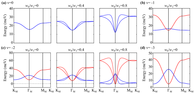
Figure 5: Exact charge $+1$ (blue) and $-1$ (red) excitations at $\theta=1.05^{\circ}$. The flat metric condition is not imposed. In this plot we have used the parameters defined in App. A: $v_{F}=5.944{\rm eV\cdot\mathring{A}}$, $|K|=1.703\mathring{\rm A}^{-1}$, $w_{1}=110{\rm meV}$, $U_{\xi}=26$meV, $\xi=10$nm. Note that the excitation gap is largely reduced from the flat-condition limit.

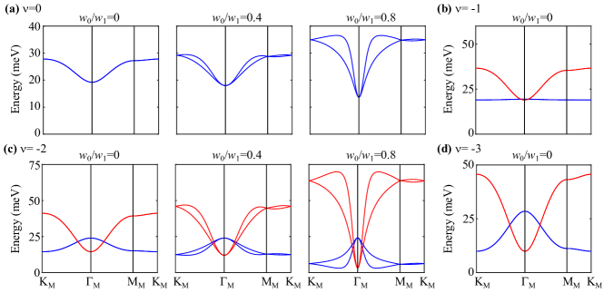
Figure 6: Exact charge $+1$ (blue) and $-1$ (red) excitations at $\theta=1.05^{\circ}$. The flat metric condition is not imposed. In this plot we set the screening length as $\xi=20$nm and accordingly the interaction strength as $U_{\xi}=13$meV. The other parameters are same as in App. A: $v_{F}=5.944{\rm eV\cdot\mathring{A}}$, $|K|=1.703\mathring{\rm A}^{-1}$, $w_{1}=110{\rm meV}$.

C.4 Charge $\pm 1$ excitation spectra for different parameters

Before we present the numerical results, let us first explain how we choose the chemical potential in the cases without assuming flat-metric-condition. First, the sum of the lowest charge +1 ($\Delta_{+}$) and charge -1 ($\Delta_{-}$) gaps do not depend on the chemical potential since upon adding a $-\delta\mu N$ term the two gaps change by $-\delta\mu$ and $\delta\mu$, respectively. Then we choose the chemical potential such that $\Delta_{+}=\Delta_{-}$. In a band structure picture, $\Delta_{+}$ is the lowest conduction band energy and $-\Delta_{-}$ is the highest valence band energy. The condition $\Delta_{+}=\Delta_{-}$ simply means that the chemical potential locates at the middle of conduction and valence bands.

In Figs. 5 and 6 the charge $\pm 1$ excitations are plotted at different fillings and $w_{0}/w_{1}$’s for two different screening lengths of the Coulomb interaction (Eq. 48), i.e., $\xi$=10nm, 20nm, respectively. The corresponding interaction strengths are $U_{\rm 10nm}=$26meV, $U_{\rm 20nm}$=13meV. We have used $w_{1}$=110meV in all the calculations and $w_{0}/w_{1}=$0, 0.4, 0.8 for $\nu=0,-2$ and $w_{0}/w_{1}=0$ for $\nu=-1,-3$.

For $\nu=0$ and $\xi=$10nm, 20nm, the charge $\pm 1$ gaps are at the $\Gamma_{M}$ momentum and are always larger than 10meV for different $w_{0}/w_{1}$’s. For $\nu=-2$ and $\xi=$20nm, the charge $\pm 1$ gaps are always larger than 5meV for different $w_{0}/w_{1}$’s. For $\nu=-2$ and $\xi=$10nm, the charge $\pm 1$ gaps are finite for $w_{0}/w_{1}=0,0.4$ but become negative at $w_{0}/w_{1}=0.8$ (Fig. 5c). We find that the gaps close around $w_{0}/w_{1}\approx 0.75$, implying that, with $\xi$=10nm and the other parameters we have used, the ground states in Eq. 8 become unstable for $w_{0}/w_{1}\approx 0.75$.

The instability shown in Fig. 5c will lead to a metallic phase at $\nu=-2$ in the nonchiral-flat limit with strong chiral symmetry breaking ($w_{0}/w_{1}=0.8$). In the band structure picture, we can understand the charge +1 excitation as the conduction band and the charge -1 excitation as the reverted valence band. The negativities of both imply that the energy of conduction band overlaps with the energy of valence band. Since we have chosen to fully occupy the valence bands, the ground state energy is not minimized in this case: One can move one particle from the top of valence band to bottom of conduction band to lower the energy. The ground state energy will be minimized by redistributing electrons to occupy the bands below the chemical potential. Due to the overlap between conduction and valence bands, the redistributed band structure will have electron and hole pockets and hence is a metallic state. In the resulted metallic phase at $\nu=-2$, there are two fully empty valley-spin sectors and two partially filled valley-spin sectors. The partially filled sectors contribute to the electron and hole pockets. This state is still invariant under a U(2) subgroup within the fully empty valley-spin sectors. Since U(4) and U(2) have 16 and 4 parameters, there will be $\frac{16-4}{2}=6$ Goldstone modes.

Appendix D Charge neutral excitations and the Goldstone stiffness

While the charge $\pm 1$ excitations can be obtained by diagonalizing a $2\times 2$ matrix, we can obtain the charge neutral, 2-body excitations above the ground state. These can be obtained by diagonalizing a $2N_{M}\times 2N_{M}$ matrix, or a one-body problem, despite the state having a thermodynamic number of particles. Due to the fact that we know the exact eigenstates (or ground states) of the system, building excitations of the Hamiltonian on top of these eigenstates (or ground states) becomes a problem of diagonalizing a basis formed only from the excitations. We now obtain the charge neutral excitations, show that they exhibit Goldstone modes with quadratic dispersion - as required by U(4) (or U(4) $\times$ U(4)) ferromagnetism, and obtain the stiffness of the Goldstone dispersion in the first chiral limit.

D.1 Exact charge neutral excitations in the nonchiral-flat U(4) limit

We choose a basis for the neutral excitations

$$c_{\mathbf{k}_{2},m_{2},\eta_{2},s_{2}}^{\dagger}c_{\mathbf{k}_{1},m_{1},\eta_{1},s_{1}}|\Psi\rangle$$ (105)

where $|\Psi\rangle$ is any of the exact ground states and/or eigenstates in Eqs. 73 and 76. The scattering matrix of this basis can be solved as easily as a one-body problem, despite the fact that Eqs. 73 and 76 hold a thermodynamic number of particles. We first have to compute the commutators:

$$[O_{\mathbf{-q,-G}}O_{\mathbf{q,G}},c_{\mathbf{k}_{2},m_{2},\eta_{2},s_{2}}^{\dagger}c_{\mathbf{k}_{1},m_{1},\eta_{1},s_{1}}]$$

$$= [O_{\mathbf{-q,-G}}O_{\mathbf{q,G}},c_{\mathbf{k}_{2},m_{2},\eta_{2},s_{2}}^{\dagger}]c_{\mathbf{k}_{1},m_{1},\eta_{1},s_{1}}+c_{\mathbf{k}_{2},m_{2},\eta_{2},s_{2}}^{\dagger}[O_{\mathbf{-q,-G}}O_{\mathbf{q,G}},c_{\mathbf{k}_{1},m_{1},\eta_{1},s_{1}}],$$ (106)

which, in detail reads:

$$[O_{\mathbf{-q,-G}}O_{\mathbf{q,G}},c_{\mathbf{k}_{2},m_{2},\eta_{2},s_{2}}^{\dagger}c_{\mathbf{k}_{1},m_{1},\eta_{1},s_{1}}]$$

$$=\sum_{m}P_{mm_{2}}^{\left(\eta_{2}\right)}\left(\mathbf{k}_{2},\mathbf{q}+\mathbf{G}\right)c_{\mathbf{k}_{2},m,\eta_{2},s_{2}}^{\dagger}c_{\mathbf{k}_{1},m_{1},\eta_{1},s_{1}}+\sum_{m}P_{m_{1}m}^{\left(\eta_{1}\right)}\left(\mathbf{k}_{1},-\mathbf{q}-\mathbf{G}\right)c_{\mathbf{k}_{2},m_{2},\eta_{2},s_{2}}^{\dagger}c_{\mathbf{k}_{1},m,\eta_{1},s_{1}}$$

$$+\sqrt{V(\mathbf{G}+\mathbf{q})}\sum_{m}\left(M_{m,m_{2}}^{\left(\eta_{2}\right)}\left(\mathbf{k}_{2},\mathbf{q}+\mathbf{G}\right)c_{\mathbf{k}_{2}+\mathbf{q},m,\eta_{2},s_{2}}^{\dagger}c_{\mathbf{k}_{1},m_{1},\eta_{1},s_{1}}O_{-\mathbf{q,-G}}+(\mathbf{q},\mathbf{G}\leftrightarrow-\mathbf{q},-\mathbf{G})\right)$$

$$-\sqrt{V(\mathbf{G}+\mathbf{q})}\sum_{m}\left(M_{m,m_{1}}^{\left(\eta_{1}\right)*}\left(\mathbf{k}_{1},-\mathbf{q}-\mathbf{G}\right)c_{\mathbf{k}_{2},m_{2},\eta_{2},s_{2}}^{\dagger}c_{\mathbf{k}_{1}-\mathbf{q},m,\eta_{1},s_{1}}O_{-\mathbf{q,-G}}+(\mathbf{q},\mathbf{G}\leftrightarrow-\mathbf{q},-\mathbf{G})\right)$$

$$-V(\mathbf{G}+\mathbf{q})\sum_{m,m^{\prime}}\left(M_{m,m_{2}}^{\left(\eta_{2}\right)}\left(\mathbf{k}_{2},\mathbf{q}+\mathbf{G}\right)M_{m^{\prime},m_{1}}^{\left(\eta_{1}\right)*}\left(\mathbf{k}_{1},\mathbf{q}+\mathbf{G}\right)c_{\mathbf{k}_{2}+\mathbf{q},m,\eta_{2},s_{2}}^{\dagger}c_{\mathbf{k}_{1}+\mathbf{q},m^{\prime},\eta_{1},s_{1}}+(\mathbf{q},\mathbf{G}\leftrightarrow-\mathbf{q},-\mathbf{G})\right)$$ (107)

By rewriting $\mathbf{k}_{2}=\mathbf{k}+\mathbf{p}$ and $\mathbf{k}_{1}=\mathbf{k}$, we can write the scattering equation as

$$\left[H_{I}-\mu N,c_{\mathbf{k}+\mathbf{p},m_{2},\eta_{2},s_{2}}^{\dagger}c_{\mathbf{k},m_{1},\eta_{1},s_{1}}\right]|\Psi\rangle=\frac{1}{2\Omega_{\text{tot}}}\sum_{m,m^{\prime}}\sum_{\mathbf{q}}S^{(\eta_{2},\eta_{1})}_{mm^{\prime};m_{2}m_{1}}(\mathbf{k}+\mathbf{q},\mathbf{k};\mathbf{p})c_{\mathbf{k}+\mathbf{p}+\mathbf{q},m,\eta_{2},s_{2}}^{\dagger}c_{\mathbf{k}+\mathbf{q},m^{\prime},\eta_{1},s_{1}}|\Psi\rangle\ .$$ (108)

The $|\Psi\rangle$ are the states $|\Psi_{\nu}\rangle$ in Eq. 76, and hence $\eta_{1},s_{1}$ belong to the valley-spin flavor/s which are fully occupied, while $\eta_{2},s_{2}$ belong to the valley/spin flavor which are not occupied.

For a generic exact eigenstate $|\Psi\rangle$ at chemical potential $\mu$ satisfying $(O_{\mathbf{q,G}}-A_{\mathbf{G}}N_{M}\delta_{\mathbf{q},0})|\Psi\rangle=0$ for some coefficient $A_{\mathbf{G}}$, we find that the scattering matrix reads

$$\begin{split}S^{(\eta_{2},\eta_{1})}_{m,m^{\prime};m_{2},m_{1}}(\mathbf{k}+\mathbf{q},\mathbf{k};\mathbf{p})=&\delta_{\mathbf{q},\mathbf{0}}(\delta_{m,m_{2}}\widetilde{R}_{m^{\prime}m_{1}}^{\eta_{1}}(\mathbf{k})+\delta_{m^{\prime},m_{1}}R_{mm_{2}}^{\eta_{2}}(\mathbf{k}+\mathbf{p}))\\ &-2\sum_{\mathbf{G}}V(\mathbf{G}+\mathbf{q})M_{m,m_{2}}^{\left(\eta_{2}\right)}\left(\mathbf{k}+\mathbf{p},\mathbf{q}+\mathbf{G}\right)M_{m^{\prime},m_{1}}^{\left(\eta_{1}\right)*}\left(\mathbf{k},\mathbf{q}+\mathbf{G}\right),\end{split}$$

where $R_{mn}^{\eta}(\mathbf{k}),\widetilde{R}_{mn}^{\eta}(\mathbf{k})$ are the $\pm 1$-excitation matrices in Sections C.1 and C.3. We see that the neutral energy is a sum of the two single-particle energies (first row of Section D.1) plus an interaction energy (second row of Section D.1).

The exact expression of the PH excitation spectrum allows for the determination of the Goldstone stiffness. The Goldstone of the U(4) and U(4)$\times$U(4) ferromagnetic ground states is part of the spectrum of the neutral excitation Eq. 108, and is the state at small momentum $\mathbf{p}=\mathbf{k}_{1}-\mathbf{k}_{2}$. We will solve this in the simpler, chiral limit, but it can be obtained in the general, non-chiral limit Eq. 108.

D.2 Exact charge neutral excitations in the (first) chiral-flat U(4)$\times$U(4) limit

We now consider the charge neutral excited states reachable by creating one electron-hole pair with total momentum $\mathbf{p}$ on the chiral-flat limit eigenstate $|\Psi_{\nu}^{\nu_{+},\nu_{-}}\rangle$. Assume the valley-spin flavor $\{\eta_{1},s_{1}\}$ has Chern band basis $e_{Y1}$ fully occupied and the valley-spin flavor $\{\eta_{2},s_{2}\}$ Chern band basis $e_{Y2}$ fully empty. We consider the Hilbert space of the following sets of states of momentum quantum number $\mathbf{p}$

$$|\mathbf{k+p,k},e_{Y1},e_{Y2},\eta_{2},\eta_{1},s_{2},s_{1},\Psi_{\nu}^{\nu_{+},\nu_{-}}\rangle=d^{\dagger}_{\mathbf{k+p},e_{Y2},\eta_{2},s_{2}}d_{\mathbf{k},e_{Y1},\eta_{1},s_{1}}|\Psi_{\nu}^{\nu_{+},\nu_{-}}\rangle\ ,$$ (109)

The $O_{\mathbf{q},\mathbf{G}}$ operators in the chiral limit have the simple, diagonal expression of Eq. 83, which leads to the scattering equation.

$$\left[H_{I}-\mu N,d^{\dagger}_{\mathbf{k+p},e_{Y2},\eta_{2},s_{2}}d_{\mathbf{k},e_{Y1},\eta_{1},s_{1}}\right]|\Psi\rangle=\frac{1}{2\Omega_{\text{tot}}}\sum_{\mathbf{q}}S_{e_{Y2};e_{Y1}}(\mathbf{k+q},\mathbf{k};\mathbf{p})d^{\dagger}_{\mathbf{k+p+q},e_{Y2},\eta_{2},s_{2}}d_{\mathbf{k+q},e_{Y1},\eta_{1},s_{1}}|\Psi\rangle\ .$$ (110)

The $|\Psi\rangle$ are the states $|\Psi_{\nu}^{\nu_{+},\nu_{-}}\rangle$ in Eq. 73, and hence $e_{Y1},\eta_{1},s_{1}$ belong to the valley-spin flavor/s which are fully occupied, while $e_{Y2},\eta_{2},s_{2}$ belong to the valley/spin flavor which are not occupied. The scattering matrix in the chiral limit does not depend on $\eta_{1},\eta_{2}$:

$$S_{e_{Y2};e_{Y1}}(\mathbf{k+q},\mathbf{k};\mathbf{p})=\delta_{\mathbf{q},\mathbf{0}}(R_{0}(\mathbf{k+p})+\widetilde{R}_{0}(\mathbf{k}))-2\sum_{\mathbf{G}}V(\mathbf{G}+\mathbf{q})M_{e_{Y2}}(\mathbf{k}+\mathbf{p},\mathbf{q}+\mathbf{G})M^{*}_{e_{Y1}}(\mathbf{k},\mathbf{q}+\mathbf{G})\ ,$$ (111)

where $M_{e_{Y}}(\mathbf{k},\mathbf{q}+\mathbf{G})$ is given in Eq. 61 and $R_{0}^{\eta}(\mathbf{k})$ is given in Eq. 99.

If condition Eq. 71 is satisfied, the eigenstates $|\Psi_{\nu}^{\nu_{+},\nu_{-}}\rangle$ are the ground states, and hence the states Eq. 110 are the neutral excitations on top of the ground states. Without the condition Eq. (71), only $\nu=0$ states are guaranteed to be the ground states, although the others are still eigenstates. With condition Eq. (71), we have

$$S_{e_{Y2};e_{Y1}}(\mathbf{k+q},\mathbf{k};\mathbf{p})=\delta_{\mathbf{q},\mathbf{0}}\sum_{\mathbf{G},\mathbf{q}^{\prime}}V(\mathbf{G}+\mathbf{q}^{\prime})[\alpha_{0}(\mathbf{k},\mathbf{q}^{\prime}+\mathbf{G})^{2}+\alpha_{2}(\mathbf{k},\mathbf{q}^{\prime}+\mathbf{G})^{2}+\alpha_{0}(\mathbf{k}+\mathbf{p},\mathbf{q}^{\prime}+\mathbf{G})^{2}+\alpha_{2}(\mathbf{k}+\mathbf{p},\mathbf{q}^{\prime}+\mathbf{G})^{2}]$$

$$-2\sum_{\mathbf{G}}V(\mathbf{G}+\mathbf{q})(\alpha_{0}(\mathbf{k+p,q+G})+ie_{Y2}\alpha_{2}(\mathbf{k+p,q+G}))(\alpha_{0}(\mathbf{k,q+G})-ie_{Y1}\alpha_{2}(\mathbf{k,q+G}))$$ (112)

Solving Eq. 110 provides us with the expression for the neutral excitations at momentum $\mathbf{p}$ on top of the TBG ground states.

D.3 Goldstone mode in the first chiral limit and the Goldstone stiffness

We show that the Goldstone mode of the ferromagnetic ground states are included in the neutral excitations of Eq. 110 and we obtain their dispersion relation, in terms of the quantum geometry factors of the TBG. We are able to analytically obtain the Goldstone mode if the condition Eq. 71 holds. We first show the presence of an exact zero eigenstate of Eq. 110.

D.3.1 Exact zero energy neutral mode Eigenstate

We now show that Eq. 110 has an exact zero energy eigenstate. In order to see this, we remark that the $\mathbf{p}=0,e_{Y1}=e_{Y2}$ state Section D.2 has a scattering matrix

$$S_{e_{Y};e_{Y}}(\mathbf{k+q},\mathbf{k};\mathbf{0})=2\delta_{\mathbf{q},\mathbf{0}}\sum_{\mathbf{G},\mathbf{q}^{\prime}}V(\mathbf{G}+\mathbf{q}^{\prime})[\alpha_{0}(\mathbf{k},\mathbf{q}^{\prime}+\mathbf{G})^{2}+\alpha_{2}(\mathbf{k},\mathbf{q}^{\prime}+\mathbf{G})^{2}]$$

$$-2\sum_{\mathbf{G}}V(\mathbf{G}+\mathbf{q})(\alpha_{0}(\mathbf{k,q+G})^{2}+\alpha_{2}(\mathbf{k,q+G})^{2})\,$$ (113)

whose elements in every row sums to zero (irrespective of $\eta_{1,2},s_{1,2}$):

$$\sum_{\mathbf{q}}S_{e_{Y};e_{Y}}(\mathbf{k+q},\mathbf{k};\mathbf{0})=0\ .$$ (114)

This guarantees that the rank of the scattering matrix is not maximal, and that there is at least one zero energy eigenstate, with equal amplitude on every $|\mathbf{k,k},e_{Y},e_{Y},\eta_{2},\eta_{1},s_{2},s_{1},\Psi_{\nu}^{\nu_{+},\nu_{-}}\rangle$

$$|e_{Y},e_{Y},\eta_{2},\eta_{1},s_{2},s_{1}\rangle=\sum_{\mathbf{q}}d^{\dagger}_{\mathbf{k+q},e_{Y},\eta_{2},s_{2}}d_{\mathbf{k+q},e_{Y},\eta_{1},s_{1}}|\Psi_{\nu}^{\nu_{+},\nu_{-}}\rangle\ ,\;\;(H_{I}-\mu N)|e_{Y},e_{Y},\eta_{2},\eta_{1},s_{2},s_{1}\rangle=0$$ (115)

A U(4)$\times$U(4) multiplet of this state is also at zero energy. Moreover, the scattering matrix $S_{e_{Y};e_{Y}}(\mathbf{k+q},\mathbf{k};0)$ is positive semidefinite (as it should, since these eigenvalues are energies of excitations on top of the ground states). For the matrix $S_{e_{Y};e_{Y}}(\mathbf{k+q},\mathbf{k};0)$, we prove that its negative, $-S_{e_{Y};e_{Y}}(\mathbf{k+q},\mathbf{k};0)$, has only non-positive eigenvalues, and hence $S_{e_{Y};e_{Y}}(\mathbf{k+q},\mathbf{k};0)$ has only non-negative eigenvalues. For $-S_{e_{Y};e_{Y}}(\mathbf{k+q},\mathbf{k};0)$, the diagonal elements $-S_{e_{Y};e_{Y}}(\mathbf{k},\mathbf{k};0)$ are non-positive, while the off-diagonal elements $-S_{e_{Y};e_{Y}}(\mathbf{k+q},\mathbf{k};0)$ ($\mathbf{q}\neq 0$) are non-negative. Hence by the Gershgorin circle theorem, all eigenvalues lie in at least one of the Gershgorin disks (which, due to the fact that the matrix is Hermitian, are intervals) centered at $-S_{e_{Y};e_{Y}}(\mathbf{k},\mathbf{k};0)$ and with radius $-\sum_{\mathbf{q}\neq 0}S_{e_{Y};e_{Y}}(\mathbf{k+q},\mathbf{k};0)$. These intervals are:

$$[-S_{e_{Y};e_{Y}}(\mathbf{k},\mathbf{k};0)+\sum_{\mathbf{q}\neq 0}S_{e_{Y};e_{Y}}(\mathbf{k}+\mathbf{q},\mathbf{k};0),-S_{e_{Y};e_{Y}}(\mathbf{k},\mathbf{k};0)-\sum_{\mathbf{q}\neq 0}S_{e_{Y};e_{Y}}(\mathbf{k+q},\mathbf{k};0)]=$$

$$=[2\sum_{\mathbf{q}\neq 0}S_{e_{Y};e_{Y}}(\mathbf{k+q},\mathbf{k};0),0].$$ (116)

Since $\sum_{\mathbf{q}\neq 0}S_{e_{Y};e_{Y}}(\mathbf{k+q},\mathbf{k};0)\leq 0,\;\;\forall\mathbf{k}$, all eigenvalues of $-S_{e_{Y};e_{Y}}(\mathbf{k+q},\mathbf{k};0)$ are non-positive, and hence all eigenvalues of $S_{e_{Y};e_{Y}}(\mathbf{k+q},\mathbf{k};0)$ are non-negative.

D.3.2 Goldstone stiffness

Since the $\mathbf{p}=0$ state has zero energy, for small $\mathbf{p}$, there will be low-energy states in the neutral continuum. By using the $\mathbf{p}=0$ states in Eq. 115, one can compute their dispersion. First, we write the Hamiltonian matrix elements acting on the two particle states

$$\langle\mathbf{k^{\prime}+p,k^{\prime}},e_{Y1}^{\prime},e_{Y2}^{\prime},\eta_{2}^{\prime},\eta_{1}^{\prime},s_{2}^{\prime},s_{1}^{\prime},\Psi_{\nu}^{\nu_{+},\nu_{-}}|H_{I}|\mathbf{k+p,k},e_{Y1},e_{Y2},\eta_{2},\eta_{1},s_{2},s_{1},\Psi_{\nu}^{\nu_{+},\nu_{-}}\rangle$$

$$=\delta_{e_{Y1}^{\prime},e_{Y2}^{\prime},\eta_{2}^{\prime},\eta_{1}^{\prime},s_{2}^{\prime},s_{1};e_{Y1},e_{Y2},\eta_{2},\eta_{1},s_{2},s_{1}}\frac{1}{2\Omega_{\text{tot}}}(\delta_{\mathbf{k}^{\prime},\mathbf{k}}S_{e_{Y2};e_{Y1}}(\mathbf{k},\mathbf{k};\mathbf{p}))-S_{e_{Y2};e_{Y1}}(\mathbf{k}^{\prime},\mathbf{k};\mathbf{p}))\ .$$ (117)

Hence, for small $\mathbf{p}$, the energy of the Goldstone mode is given by the expectation value

$$E_{\text{Goldstone}}(\mathbf{p})= \sum_{\mathbf{k},\mathbf{k}^{\prime}}\langle\mathbf{k^{\prime}+p,k^{\prime}},e_{Y},e_{Y},\eta_{2},\eta_{1},s_{2},s_{1},\Psi_{\nu}^{\nu_{+},\nu_{-}}|H_{I}|\mathbf{k+p,k},e_{Y},e_{Y},\eta_{1},\eta_{1},s_{2},s_{1},\Psi_{\nu}^{\nu_{+},\nu_{-}}\rangle$$

$$= \frac{1}{2\Omega_{\text{tot}}}\sum_{k}\left(S_{e_{Y};e_{Y}}(\mathbf{k},\mathbf{k};\mathbf{p})-\sum_{\mathbf{q}}S_{e_{Y};e_{Y}}(\mathbf{k+q},\mathbf{k};\mathbf{p})\right)\ .$$ (118)

As expected for the Goldstone of a ferromagnet, the linear term in $\mathbf{p}$ vanishes; by using $\alpha_{a}(\mathbf{k},\mathbf{q}+\mathbf{G})=\alpha_{a}(-\mathbf{k},-\mathbf{q}-\mathbf{G})\quad\text{for }a=0,2$ of Eq. 54, we find can prove that the linear terms vanish exactly. To second order in $\mathbf{p}$, we find the Goldtone stiffness

$$E_{\text{Goldstone}}(\mathbf{p})=\frac{1}{2}m_{ij}p_{i}p_{j},$$ (119)

$$m_{ij}= \frac{1}{2\Omega_{\text{tot}}}\sum_{\mathbf{k},\mathbf{q},\mathbf{G}}V(\mathbf{G}+\mathbf{q})[\alpha_{0}(\mathbf{k},\mathbf{q}+\mathbf{G})\partial_{k_{i}}\partial_{k_{j}}\alpha_{0}(\mathbf{k},\mathbf{q}+\mathbf{G})+\alpha_{2}(\mathbf{k},\mathbf{q}+\mathbf{G})\partial_{k_{i}}\partial_{k_{j}}\alpha_{2}(\mathbf{k},\mathbf{q}+\mathbf{G})$$

$$+2\partial_{k_{i}}\alpha_{0}(\mathbf{k},\mathbf{q}+\mathbf{G})\partial_{k_{j}}\alpha_{0}(\mathbf{k},\mathbf{q}+\mathbf{G})+2\partial_{k_{i}}\alpha_{2}(\mathbf{k},\mathbf{q}+\mathbf{G})\partial_{k_{j}}\alpha_{2}(\mathbf{k},\mathbf{q}+\mathbf{G})]\ .$$ (120)

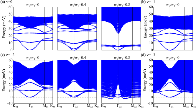
Figure 7: Exact charge neutral excitations with $\theta=1.05^{\circ}$. The flat metric condition is not imposed. In this plot we have used the parameters defined in App. A: $v_{F}=5.944{\rm eV\cdot\mathring{A}}$, $|K|=1.703\mathring{\rm A}^{-1}$, $w_{1}=110{\rm meV}$, $U_{\xi}=26$meV, $\xi=10$nm.

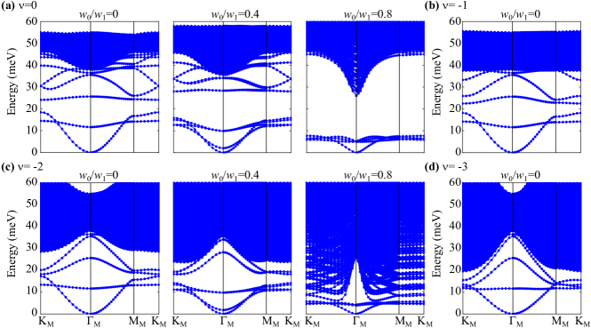
Figure 8: Exact charge neutral excitations with $\theta=1.05^{\circ}$. The flat metric condition is not imposed. In this plot we use the screening length $\xi$=20nm and $U_{\xi}=13$meV accordingly. The other parameters are same as in App. A, i.e., $v_{F}=5.944{\rm eV\cdot\mathring{A}}$, $|K|=1.703\mathring{\rm A}^{-1}$, $w_{1}=110{\rm meV}$.

D.4 Charge neutral excitation spectra for different parameters

In Figs. 7 and 8 the charge neutral excitations are plotted at different fillings and $w_{0}/w_{1}$’s for two different screening lengths of the Coulomb interaction (Eq. 48), i.e., $\xi$=10nm, 20nm, respectively. The corresponding interaction strengths are $U_{\rm 10nm}=$26meV, $U_{\rm 20nm}$=13meV. We have used $w_{1}$=110meV in all the calculations and $w_{0}/w_{1}=$0, 0.4, 0.8 for $\nu=0,-2$ and $w_{0}/w_{1}=0$ for $\nu=-1,-3$.

For the parameters we used, the $\nu=0$ states with $w_{0}/w_{1}=0,0.4,0.8$ and $\nu=-1,-3$ states with $w_{0}=0$ have non-negative excitations and hence are stable. The $\nu=-2$ states with $w_{0}/w_{1}=0,0.4,0.8$ are also stable for $\xi=$20nm. However, the $\nu=-2$ states for $\xi=$10nm become unstable at $w_{0}/w_{1}=0.8$ (Fig. 7c). The instability can be understood from the instability of the charge $\pm 1$ excitations shown in Fig. 5c. From Fig. 5c we can see that the charge +1 excitation is negative at some momenta between $\Gamma_{M}$ and $K_{M}$ and the charge -1 excitation is negative at $\Gamma_{M}$. Combining a pair of these negative particle and hole one obtains a negative charge neutral excitation. As discussed in the end of Section C.4, this instability will lead to a metallic phase.

For the stable ground states, where the spectrum is non-negative, the charge neutral spectrum consists of a particle-hole continuum (the blue area in Figs. 7 and 8) and a set of gapped collective modes. In Figs. 7 and 8 we only plot the eigenvalues of the scattering matrix. In practice, the existence and degeneracy of an excitation mode also depend on the occupied U(4) flavors (and U(4)$\times$U(4) flavors in the first chiral limit) of the ground state, as discussed in Section III.1. In particular, the number of Goldstone modes for different ground states are given in Tables 2 and 1. In general, the states $|\Psi_{\nu}^{\nu_{+},\nu_{-}}\rangle$ (Eq. 10) in the (first) chiral-flat U(4)$\times$U(4) limit with $\nu=0,\pm 2$ and $\nu_{+}=\nu_{-}=\frac{\nu+4}{2}$ (such that it has vanishing Chern number) has more Goldstone modes than the state $|\Psi_{\nu}\rangle$ (Eq. 8) with the same filling $\nu$. From $w_{0}/w_{1}=0.4$ to $w_{0}/w_{1}=0$ for the states at $\nu=0,-2$ we can clearly see in Figs. 7 and 8 that a collective mode is soften and become Goldstone mode, consistent with the theoretical analysis.

Appendix E Charge $\pm 2$ excitations and conditions on Cooper pair instability

The charge $\pm 1$ excitations can be obtained by diagonalizing a $2\times 2$ matrix; the charge neutral above the ground state can be obtained by diagonalizing a $2N_{M}\times 2N_{M}$ matrix, or a one-body problem, despite the state having a thermodynamic number of particles, due to the fact that we know the exact eigenstates (or ground states) of the system. We now show that the charge $+2$ excitations can also be obtained by diagonalizing a $2N_{M}\times 2N_{M}$ matrix. The conditions for which Cooper pairing occurs are also obtained.

E.1 Charge $+2$ excitations in the nonchiral-flat U(4) limit

We choose a basis for the neutral excitations

$$c_{\mathbf{k}_{2},m_{2},\eta_{2},s_{2}}^{\dagger}c^{\dagger}_{\mathbf{k}_{1},m_{1},\eta_{1},s_{1}}|\Psi\rangle$$ (121)

where $|\psi\rangle$ is any of the exact ground states/eigenstates Eqs. 73 and 76. The scattering matrix of these basis can be solved as easily as a one-body problem. We first have to compute the commutators:

$$[O_{\mathbf{-q,-G}}O_{\mathbf{q,G}},c_{\mathbf{k}_{2},m_{2},\eta_{2},s_{2}}^{\dagger}c^{\dagger}_{\mathbf{k}_{1},m_{1},\eta_{1},s_{1}}]$$

$$= [O_{\mathbf{-q,-G}}O_{\mathbf{q,G}},c_{\mathbf{k}_{2},m_{2},\eta_{2},s_{2}}^{\dagger}]c^{\dagger}_{\mathbf{k}_{1},m_{1},\eta_{1},s_{1}}+c_{\mathbf{k}_{2},m_{2},\eta_{2},s_{2}}^{\dagger}[O_{\mathbf{-q,-G}}O_{\mathbf{q,G}},c^{\dagger}_{\mathbf{k}_{1},m_{1},\eta_{1},s_{1}}]\ ,$$ (122)

which, in detail reads:

$$[O_{\mathbf{-q,-G}}O_{\mathbf{q,G}},c_{\mathbf{k}_{2},m_{2},\eta_{2},s_{2}}^{\dagger}c^{\dagger}_{\mathbf{k}_{1},m_{1},\eta_{1},s_{1}}]$$

$$=\sum_{m}P_{mm_{2}}^{\left(\eta_{2}\right)}\left(\mathbf{k}_{2},\mathbf{q}+\mathbf{G}\right)c_{\mathbf{k}_{2},m,\eta_{2},s_{2}}^{\dagger}c^{\dagger}_{\mathbf{k}_{1},m_{1},\eta_{1},s_{1}}+\sum_{m}P_{mm_{1}}^{\left(\eta_{1}\right)}\left(\mathbf{k}_{1},\mathbf{q}+\mathbf{G}\right)c_{\mathbf{k}_{2},m_{2},\eta_{2},s_{2}}^{\dagger}c^{\dagger}_{\mathbf{k}_{1},m,\eta_{1},s_{1}}$$

$$+\sqrt{V(\mathbf{G}+\mathbf{q})}\sum_{m}\left(M_{m,m_{2}}^{\left(\eta_{2}\right)}\left(\mathbf{k}_{2},\mathbf{q}+\mathbf{G}\right)c_{\mathbf{k}_{2}+\mathbf{q},m,\eta_{2},s_{2}}^{\dagger}c^{\dagger}_{\mathbf{k}_{1},m_{1},\eta_{1},s_{1}}O_{-\mathbf{q,-G}}+(\mathbf{q},\mathbf{G}\leftrightarrow-\mathbf{q},-\mathbf{G})\right)$$

$$+\sqrt{V(\mathbf{G}+\mathbf{q})}\sum_{m}\left(M_{m,m_{1}}^{\left(\eta_{1}\right)}\left(\mathbf{k}_{1},\mathbf{q}+\mathbf{G}\right)c_{\mathbf{k}_{2},m_{2},\eta_{2},s_{2}}^{\dagger}c^{\dagger}_{\mathbf{k}_{1}+\mathbf{q},m,\eta_{1},s_{1}}O_{-\mathbf{q,-G}}+(\mathbf{q},\mathbf{G}\leftrightarrow-\mathbf{q},-\mathbf{G})\right)$$

$$+V(\mathbf{G}+\mathbf{q})\sum_{m,m^{\prime}}\left(M_{m,m_{2}}^{\left(\eta_{2}\right)}\left(\mathbf{k}_{2},\mathbf{q}+\mathbf{G}\right)M_{m^{\prime},m_{1}}^{\left(\eta_{1}\right)}\left(\mathbf{k}_{1},-\mathbf{q}-\mathbf{G}\right)c_{\mathbf{k}_{2}+\mathbf{q},m,\eta_{2},s_{2}}^{\dagger}c^{\dagger}_{\mathbf{k}_{1}-\mathbf{q},m^{\prime},\eta_{1},s_{1}}+(\mathbf{q},\mathbf{G}\leftrightarrow-\mathbf{q},-\mathbf{G})\right)$$ (123)

By rewriting $\mathbf{k}_{2}=\mathbf{k}+\mathbf{p}$ and $\mathbf{k}_{1}=-\mathbf{k}$, we can write the scattering equation as

$$\left[H_{I}-\mu N,c_{\mathbf{k}+\mathbf{p},m_{2},\eta_{2},s_{2}}^{\dagger}c^{\dagger}_{-\mathbf{k},m_{1},\eta_{1},s_{1}}\right]|\Psi\rangle=\frac{1}{2\Omega_{\text{tot}}}\sum_{m,m^{\prime}}\sum_{\mathbf{q}}T^{(\eta_{2},\eta_{1})}_{mm^{\prime};m_{2}m_{1}}(\mathbf{k}+\mathbf{q},\mathbf{k};\mathbf{p})c_{\mathbf{k}+\mathbf{p}+\mathbf{q},m,\eta_{2},s_{2}}^{\dagger}c^{\dagger}_{-\mathbf{k}-\mathbf{q},m^{\prime},\eta_{1},s_{1}}|\Psi\rangle\ ,$$ (124)

The $|\Psi\rangle$ are the states $|\Psi_{\nu}\rangle$ in Eq. 76, and hence $\eta_{1},s_{1},\eta_{2},s_{2}$ belong to the valley/spin flavor which are not occupied. For a generic exact eigenstate $|\Psi\rangle$ at chemical potential $\mu$ satisfying $(O_{\mathbf{q,G}}-A_{\mathbf{G}}N_{M}\delta_{\mathbf{q},0})|\Psi\rangle=0$ for some coefficient $A_{\mathbf{G}}$, we find that the $T^{(\eta_{2},\eta_{1})}_{m_{2},m;m_{1}m^{\prime}}(\mathbf{k}_{1},\mathbf{k}_{2};\mathbf{q})$ matrix reads

$$T^{(\eta_{2},\eta_{1})}_{mm^{\prime};m_{2}m_{1}}(\mathbf{k}+\mathbf{q},\mathbf{k};\mathbf{p})= \delta_{\mathbf{q},\mathbf{0}}(\delta_{m,m_{2}}R_{m^{\prime}m_{1}}^{\eta_{1}}(-\mathbf{k})+\delta_{m^{\prime},m_{1}}R_{mm_{2}}^{\eta_{2}}(\mathbf{k}+\mathbf{p}))+$$

$$+2\sum_{\mathbf{G}}V(\mathbf{G}+\mathbf{q})M_{m,m_{2}}^{\left(\eta_{2}\right)}\left(\mathbf{k}+\mathbf{p},\mathbf{q}+\mathbf{G}\right)M_{m^{\prime},m_{1}}^{\left(\eta_{1}\right)}\left(-\mathbf{k},-\mathbf{q}-\mathbf{G}\right)\ ,$$ (125)

where $R_{mn}^{\eta}(\mathbf{k}),R_{mn}^{\eta}(\mathbf{k})$ are the $+1$ excitation matrices in Sections C.1 and C.3. We see that the charge $+2$ energy is a sum of the two single-particle energies (first row of Section D.1) plus an interaction energy (second row of Section D.1).

The exact expression of the charge $+2$ excitation spectrum allows for the determination of the Cooper pair binding energy (if any).

E.2 Charge $+2$ excitations in the (first) chiral-flat U(4)$\times$U(4) limit

We now consider the charge $+2$ excited states reachable by creating two electron pair with total momentum $\mathbf{p}$ on the chiral-flat limit eigenstate $|\Psi_{\nu}^{\nu_{+},\nu_{-}}\rangle$. Assume the valley-spin flavor $\{\eta_{1,2},s_{1,2}\}$ has Chern band basis $e_{Y1},e_{Y2}$ fully empty. We consider the Hilbert space of the following sets of states of momentum quantum number $\mathbf{p}$ ($\mathbf{k}_{2}=-\mathbf{k}_{1}+\mathbf{p},\;\mathbf{k}_{1}=\mathbf{k}$):

$$|\mathbf{k+p,-k},e_{Y1},e_{Y2},\eta_{2},\eta_{1},s_{2},s_{1},\Psi_{\nu}^{\nu_{+},\nu_{-}}\rangle=d^{\dagger}_{\mathbf{k+p},e_{Y2},\eta_{2},s_{2}}d^{\dagger}_{-\mathbf{k},e_{Y1},\eta_{1},s_{1}}|\Psi_{\nu}^{\nu_{+},\nu_{-}}\rangle\ ,$$ (126)

The $O_{\mathbf{q},\mathbf{G}}$ operators in the chiral limit have the simple, diagonal expression of Eq. 83, which leads to the scattering equation.

$$\left[H_{I}-\mu N,d^{\dagger}_{\mathbf{k+p},e_{Y2},\eta_{2},s_{2}}d^{\dagger}_{-\mathbf{k},e_{Y1},\eta_{1},s_{1}}\right]|\Psi\rangle=\frac{1}{2\Omega_{\text{tot}}}\sum_{\mathbf{q}}T_{e_{Y2};e_{Y1}}(\mathbf{k+q},\mathbf{k};\mathbf{p})d^{\dagger}_{\mathbf{k+p+q},e_{Y2},\eta_{2},s_{2}}d^{\dagger}_{\mathbf{-k-q},e_{Y1},\eta_{1},s_{1}}|\Psi\rangle\ .$$ (127)

The $|\Psi\rangle$ are the states $|\Psi_{\nu}^{\nu_{+},\nu_{-}}\rangle$ in Eq. 73, and hence $e_{Y1},\eta_{1},s_{1}$, $e_{Y2},\eta_{2},s_{2}$ belong to the valley/spin flavor which are not occupied. The scattering matrix in the first chiral limit does not depend on $\eta_{1},\eta_{2}$

$$T_{e_{Y2};e_{Y1}}(\mathbf{k+q},\mathbf{k};\mathbf{p})=\delta_{\mathbf{q},0}(R_{0}(\mathbf{k+p})+R_{0}(-\mathbf{k}))+2\sum_{\mathbf{G}}V(\mathbf{G}+\mathbf{q})M_{e_{Y2}}(\mathbf{k}+\mathbf{p},\mathbf{q}+\mathbf{G})M_{e_{Y1}}(-\mathbf{k},-\mathbf{q}-\mathbf{G})\ ,$$ (128)

where $M_{e_{Y}}(\mathbf{k},\mathbf{q}+\mathbf{G})$ is given in Eq. 61 and $R_{0}^{\eta}(\mathbf{k})$ is given in Eq. 99.

If condition Eq. 71 is satisfied, the eigenstates $|\Psi_{\nu}^{\nu_{+},\nu_{-}}\rangle$ are the ground states, and hence the states Eq. 127 are the neutral excitations on top of the ground states. Without Eq. 71, only $\nu=0$ states are guaranteed to be the ground states, although the others are still eigenstates. With condition Eq. 71, we have

$$T_{e_{Y2};e_{Y1}}(\mathbf{k+q},\mathbf{k};\mathbf{p})=\delta_{\mathbf{q},0}\sum_{\mathbf{G},\mathbf{q}}V(\mathbf{G}+\mathbf{q})[\alpha_{0}(\mathbf{k},\mathbf{q}+\mathbf{G})^{2}+\alpha_{2}(\mathbf{k},\mathbf{q}+\mathbf{G})^{2}+\alpha_{0}(\mathbf{k}+\mathbf{p},\mathbf{q}+\mathbf{G})^{2}+\alpha_{2}(\mathbf{k}+\mathbf{p},\mathbf{q}+\mathbf{G})^{2}]$$

$$+2\sum_{\mathbf{G}}V(\mathbf{G}+\mathbf{q})(\alpha_{0}(\mathbf{k+p,q+G})+ie_{Y2}\alpha_{2}(\mathbf{k+p,q+G}))(\alpha_{0}(\mathbf{k,q+G})+ie_{Y1}\alpha_{2}(\mathbf{k,q+G}))\ ,$$ (129)

where we have used the $\alpha_{0,2}(\mathbf{k},\mathbf{q}+\mathbf{G})=\alpha_{0,2}(-\mathbf{k},-\mathbf{q}-\mathbf{G})$. Solving Eq. 127 provides us with the expression for the charge $+2$ excitations at momentum $\mathbf{p}$ on top of the TBG ground states.

E.3 Absence of Cooper pairing in the projected Coulomb Hamiltonian

In Section V.2, we have derived the sufficient conditions for the existence (Eq. 37) and absence (Eq. 38) of Cooper pairing binding energies. Now we prove that, in the projected Coulomb Hamiltonian with time-reversal symmetry $T$ and the combined symmetry $PC_{2z}T$, where $P$ is the unitary PH symmetry Song et al. (2019, 2020), $T^{(\eta_{2},\eta_{1}){\prime\prime}}_{m,m^{\prime};m_{2},m_{1}}(\mathbf{k}+\mathbf{q},\mathbf{k};\mathbf{p})$ is guaranteed to be positive semi-definite. Thus the condition Eq. (38) for the absence of Cooper pairing binding energy is always satisfied. We write $T^{(\eta_{2},\eta_{1}){\prime\prime}}_{m,m^{\prime};m_{2},m_{1}}(\mathbf{k}+\mathbf{q},\mathbf{k};\mathbf{p})$, which is defined as the third term in Section E.1, as

$$T^{(\eta_{2},\eta_{1}){\prime\prime}}_{m,m^{\prime};m_{2},m_{1}}(\mathbf{k}+\mathbf{q},\mathbf{k};\mathbf{p})=2\sum_{\mathbf{G}}V(\mathbf{G}+\mathbf{q})M_{mm_{2}}^{\left(\eta_{2}\right)}\left(\mathbf{k}+\mathbf{p},\mathbf{q}+\mathbf{G}\right)M_{m^{\prime}m_{1}}^{\left(\eta_{1}\right)}\left(-\mathbf{k},-\mathbf{q}-\mathbf{G}\right).$$ (130)

We first consider the case $\eta_{2}=-\eta_{1}=\eta$. Due to the time-reversal symmetry $T|u_{n,\eta}(-\mathbf{k})\rangle=|u_{n,-\eta}(\mathbf{k})\rangle$ in the gauge Eq. 51 Bernevig et al. (2020b), where $|u_{n,\eta}(\mathbf{k})\rangle$ is the $2N_{\mathbf{Q}}\times 1$ vector $u_{\mathbf{Q},\alpha;n\eta}(\mathbf{k})$ in Eq. 44, and the definition of the $M$ matrix (Eq. 49), we have

$$M_{mn}^{(\eta)}(\mathbf{k},\mathbf{q}+\mathbf{G})=\langle u_{m,\eta}(\mathbf{k}+\mathbf{q}+\mathbf{G})|u_{n,\eta}(\mathbf{k})\rangle=\langle Tu_{m,-\eta}(-\mathbf{k}-\mathbf{q}-\mathbf{G})|Tu_{n,-\eta}(-\mathbf{k})\rangle$$

$$= \langle u_{n,-\eta}(-\mathbf{k})|u_{m,-\eta}(-\mathbf{k}-\mathbf{q}-\mathbf{G})\rangle=\langle u_{m,-\eta}(-\mathbf{k}-\mathbf{q}-\mathbf{G})|u_{n,-\eta}(-\mathbf{k})\rangle^{*}=M_{mn}^{(-\eta)}(-\mathbf{k},-\mathbf{q}-\mathbf{G}).$$ (131)

Thus we can rewrite $T^{(\eta,-\eta){\prime\prime}}_{m,m^{\prime};m_{2},m_{1}}(\mathbf{k}+\mathbf{q},\mathbf{k};\mathbf{p})$ as

$$T^{(\eta,-\eta){\prime\prime}}_{m,m^{\prime};m_{2},m_{1}}(\mathbf{k}+\mathbf{q},\mathbf{k};\mathbf{p})=2\sum_{\mathbf{G}}V(\mathbf{G}+\mathbf{q})M_{mm_{2}}^{\left(\eta\right)}\left(\mathbf{k}+\mathbf{p},\mathbf{q}+\mathbf{G}\right)M_{m^{\prime}m_{1}}^{\left(\eta\right)*}\left(\mathbf{k},\mathbf{q}+\mathbf{G}\right).$$ (132)

We consider the expectation value of $T^{(\eta,-\eta){\prime\prime}}(\mathbf{k}+\mathbf{q},\mathbf{k};\mathbf{p})$ on a complex function $\phi_{m_{2},m_{1}}(\mathbf{k})$:

$$\langle T^{\prime\prime}\rangle^{\eta}_{\phi}(\mathbf{p})=\sum_{\mathbf{k}_{1},\mathbf{k}_{2}}\sum_{mm^{\prime}m_{2}m_{2}}\phi^{*}_{mm^{\prime}}(\mathbf{k}_{2})T^{(\eta,-\eta){\prime\prime}}(\mathbf{k}_{2},\mathbf{k}_{1};\mathbf{p})\phi_{m_{2},m_{1}}(\mathbf{k}_{1})$$

$$= 2\sum_{\mathbf{k}_{1},\mathbf{k}_{2},\mathbf{G}}V(\mathbf{k}_{2}+\mathbf{G}-\mathbf{k}_{1})\phi^{*}_{mm^{\prime}}(\mathbf{k}_{2})\langle u_{m\eta}(\mathbf{k}_{2}+\mathbf{p}+\mathbf{G})|u_{m_{2}\eta}(\mathbf{k}_{1}+\mathbf{p})\rangle\phi_{m_{2},m_{1}}(\mathbf{k}_{1})\langle u_{m_{1}}(\mathbf{k}_{1})|u_{m^{\prime}\eta}(\mathbf{k}_{2}+\mathbf{G})\rangle.$$ (133)

Using Eq. 45, we have $\langle u_{m_{1}}(\mathbf{k})|u_{m^{\prime}\eta}(\mathbf{k}+\mathbf{q}+\mathbf{G})\rangle=\langle u_{m_{1}}(\mathbf{k}+\mathbf{G}^{\prime})|u_{m^{\prime}\eta}(\mathbf{k}+\mathbf{q}+\mathbf{G}+\mathbf{G}^{\prime})\rangle$ and hence

$$\langle T^{\prime\prime}\rangle^{\eta}_{\phi}(\mathbf{p})= \frac{2}{N_{\mathbf{G}}}\sum_{\mathbf{k}_{1},\mathbf{k}_{2},\mathbf{G}_{1},\mathbf{G}_{2}}\sum_{mm^{\prime}m_{2}m_{1}}V(\mathbf{k}_{2}+\mathbf{G}_{2}-\mathbf{k}_{1}-\mathbf{G}_{1})$$

$$\times\phi^{*}_{mm^{\prime}}(\mathbf{k}_{2})\langle u_{m\eta}(\mathbf{k}_{2}+\mathbf{p}+\mathbf{G}_{2})|u_{m_{2}\eta}(\mathbf{k}_{1}+\mathbf{p}+\mathbf{G}_{1})\rangle\phi_{m_{2},m_{1}}(\mathbf{k}_{1})\langle u_{m_{1}}(\mathbf{k}_{1}+\mathbf{G}_{1})|u_{m^{\prime}\eta}(\mathbf{k}_{2}+\mathbf{G}_{2})\rangle.$$ (134)

We then define the matrix

$$W(\mathbf{k}_{1}+\mathbf{G}_{1})=\sum_{m_{2}m_{1}}|u_{m_{2}\eta}(\mathbf{k}_{1}+\mathbf{p}+\mathbf{G}_{1})\rangle\phi_{m_{2},m_{1}}(\mathbf{k}_{1})\langle u_{m_{1}}(\mathbf{k}_{1}+\mathbf{G}_{1})|$$ (135)

such that $\langle T^{\prime\prime}\rangle^{\eta}_{\phi}(\mathbf{p})$ can be written as

$$\langle T^{\prime\prime}\rangle^{\eta}_{\phi}(\mathbf{p})= \frac{2}{N_{\mathbf{G}}}\sum_{\mathbf{k}_{1},\mathbf{k}_{2},\mathbf{G}_{1},\mathbf{G}_{2}}\mathrm{Tr}[W^{\dagger}(\mathbf{k}_{2}+\mathbf{G}_{2})W(\mathbf{k}_{1}+\mathbf{G}_{1})]V(\mathbf{k}_{2}+\mathbf{G}_{2}-\mathbf{k}_{1}-\mathbf{G}_{1})$$

$$= \frac{2}{N_{\mathbf{G}}}\sum_{ab}\sum_{\mathbf{k}_{1},\mathbf{k}_{2},\mathbf{G}_{1},\mathbf{G}_{2}}W_{ab}^{*}(\mathbf{k}_{2}+\mathbf{G}_{2})W_{ab}(\mathbf{k}_{1}+\mathbf{G}_{1})V(\mathbf{k}_{2}+\mathbf{G}_{2}-\mathbf{k}_{1}-\mathbf{G}_{1}),$$ (136)

where $a,b$ are the indices of the matrix $W(\mathbf{k}+\mathbf{G})$. For each term with given $a,b$ in Eq. 136, we can view the summation over $\mathbf{k}_{1},\mathbf{k}_{2},\mathbf{G}_{1},\mathbf{G}_{2}$ as $W_{ab}^{\dagger}VW_{ab}$, where now $W_{ab}(\mathbf{k}+\mathbf{G})$ is viewed as a vector with the index $\mathbf{k}+\mathbf{G}$. Since $V(\mathbf{k}_{2}+\mathbf{G}_{2}-\mathbf{k}_{1}-\mathbf{G}_{1})$ is a positive semi-definite matrix, $W_{ab}^{\dagger}VW_{ab}$ must be non-negative, and hence $\langle T^{\prime\prime}\rangle^{\eta}_{\phi}(\mathbf{p})\geq 0$ for arbitrary $\phi$. Therefore $T^{(\eta,-\eta){\prime\prime}}_{m,m^{\prime};m_{2},m_{1}}(\mathbf{k}+\mathbf{q},\mathbf{k};\mathbf{p})$ is positive semi-definite at every $\mathbf{p}$.

Then we prove that $T^{(\eta_{2},\eta_{1}){\prime\prime}}_{m,m^{\prime};m_{2},m_{1}}(\mathbf{k}+\mathbf{q},\mathbf{k};\mathbf{p})$ with $\eta_{2}=\eta_{1}=\eta$ is also positive semi-definite. Due to the symmetry $PC_{2z}T|u_{n,\eta}(\mathbf{k})\rangle=n|u_{-n,\eta}(-\mathbf{k})\rangle$ in the gauge Eq. 51 Bernevig et al. (2020b) and the definition of the $M$ matrix (Eq. 49), we have

$$M_{mn}^{(\eta)}(\mathbf{k},\mathbf{q}+\mathbf{G})=\langle u_{m,\eta}(\mathbf{k}+\mathbf{q}+\mathbf{G})|u_{n,\eta}(\mathbf{k})\rangle=nm\langle PC_{2z}Tu_{-m,\eta}(-\mathbf{k}-\mathbf{q}-\mathbf{G})|PC_{2z}Tu_{-n,\eta}(-\mathbf{k})\rangle$$

$$= nm\langle u_{-n,\eta}(-\mathbf{k})|u_{-m,\eta}(-\mathbf{k}-\mathbf{q}-\mathbf{G})\rangle=nmM_{-m,-n}^{(\eta)*}(-\mathbf{k},-\mathbf{q}-\mathbf{G}).$$ (137)

Thus we can rewrite $T^{(\eta,\eta){\prime\prime}}_{m,m^{\prime};m_{2},m_{1}}(\mathbf{k}+\mathbf{q},\mathbf{k};\mathbf{p})$ as

$$T^{(\eta,\eta){\prime\prime}}_{m,m^{\prime};m_{2},m_{1}}(\mathbf{k}+\mathbf{q},\mathbf{k};\mathbf{p})=2\sum_{\mathbf{G}}V(\mathbf{G}+\mathbf{q})M_{mm_{2}}^{\left(\eta\right)}\left(\mathbf{k}+\mathbf{p},\mathbf{q}+\mathbf{G}\right)m^{\prime}m_{1}M_{-m^{\prime},-m_{1}}^{\left(\eta\right)*}\left(\mathbf{k},\mathbf{q}+\mathbf{G}\right).$$ (138)

Repeating the calculations starting from Section E.3, one can show that $T^{(\eta,\eta){\prime\prime}}_{m,m^{\prime};m_{2},m_{1}}(\mathbf{k}+\mathbf{q},\mathbf{k};\mathbf{p})$ must be positive semi-definite. The only difference with the above proof is that the definition of the $W$ matrix becomes

$$W(\mathbf{k}_{1}+\mathbf{G}_{1})=\sum_{m_{2}m_{1}}|u_{m_{2}\eta}(\mathbf{k}_{1}+\mathbf{p}+\mathbf{G}_{1})\rangle\phi_{m_{2},m_{1}}(\mathbf{k}_{1})\langle u_{-m_{1}}(\mathbf{k}_{1}+\mathbf{G}_{1})|m_{1}.$$ (139)

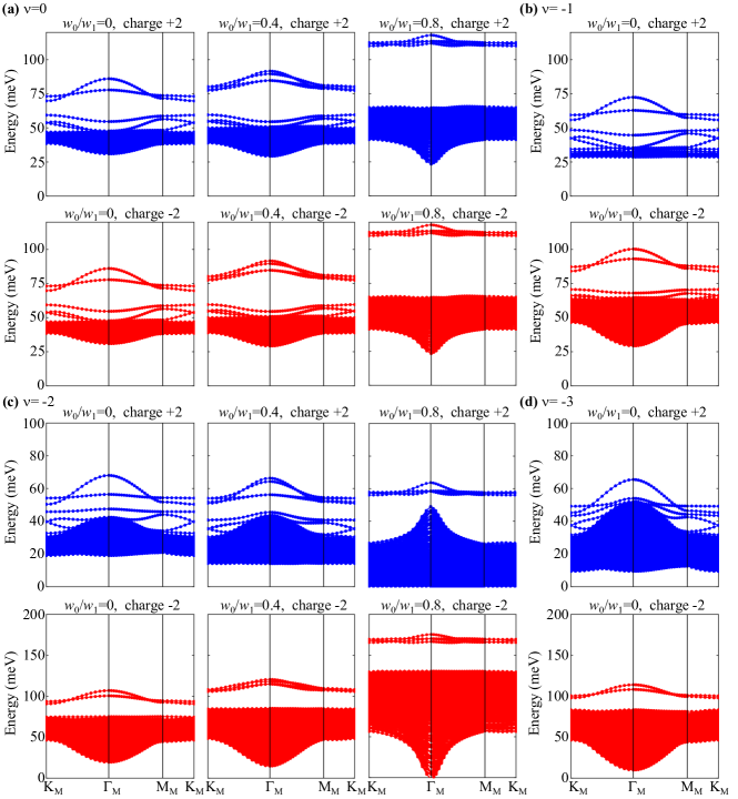
Figure 9: Exact charge $+2$ (blue) and $-2$ (red) excitations at $\theta=1.05^{\circ}$. The flat metric condition is not imposed. In this plot we have used the parameters defined in App. A: $v_{F}=5.944{\rm eV\cdot\mathring{A}}$, $|K|=1.703\mathring{\rm A}^{-1}$, $w_{1}=110{\rm meV}$, $U_{\xi}=26$meV, $\xi=10$nm.

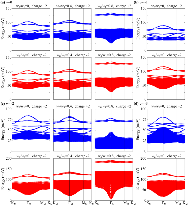
Figure 10: Exact charge $+2$ (blue) and $-2$ (red) excitations at $\theta=1.05^{\circ}$. The flat metric condition is not imposed. In this plot we use the screening length $\xi=$20nm and the interaction strength $U_{\xi}$=13meV accordingly. The other parameters are same as in App. A: $v_{F}=5.944{\rm eV\cdot\mathring{A}}$, $|K|=1.703\mathring{\rm A}^{-1}$, $w_{1}=110{\rm meV}$.

E.4 Charge $-2$ excitations

Based on the above, the charge $-2$ excitations are trivial to obtain. We do not give the details, but just the expression for the scattering elements

$$\left[H_{I}-\mu N,c_{\mathbf{k}+\mathbf{p},m_{2},\eta_{2},s_{2}}c_{-\mathbf{k},m_{1},\eta_{1},s_{1}}\right]|\Psi\rangle=\frac{1}{2\Omega_{\text{tot}}}\sum_{m,m^{\prime}}\sum_{\mathbf{q}}\widetilde{T}^{(\eta_{2},\eta_{1})}_{mm^{\prime};m_{2}m_{1}}(\mathbf{k+q},\mathbf{k};\mathbf{p})c_{\mathbf{k}+\mathbf{p}+\mathbf{q},m,\eta_{2},s_{2}}c_{-\mathbf{k}-\mathbf{q},m^{\prime},\eta_{1},s_{1}}|\Psi\rangle\ ,$$ (140)

The $|\Psi\rangle$ are the states $|\Psi_{\nu}\rangle$ in Eq. 76, and hence $\eta_{1},s_{1},\eta_{2},s_{2}$ belong to the valley/spin flavor which are not occupied. For a generic exact eigenstate $|\Psi\rangle$ at chemical potential $\mu$ satisfying $(O_{\mathbf{q,G}}-A_{\mathbf{G}}N_{M}\delta_{\mathbf{q},0})|\Psi\rangle=0$ for some coefficient $A_{\mathbf{G}}$, we find that the $\widetilde{T}^{(\eta_{2},\eta_{1})}_{m_{2},m;m_{1}m^{\prime}}(\mathbf{k}_{1},\mathbf{k}_{2};\mathbf{q})$ matrix reads

$$\widetilde{T}^{(\eta_{2},\eta_{1})}_{mm^{\prime};m_{2}m_{1}}(\mathbf{k+q},\mathbf{k};\mathbf{p})= \delta_{\mathbf{q},0}(\delta_{m,m_{2}}\widetilde{R}_{m^{\prime}m_{1}}^{\eta_{1}}(-\mathbf{k})+\delta_{m^{\prime},m_{1}}\widetilde{R}_{mm_{2}}^{\eta_{2}}(\mathbf{k}+\mathbf{p}))$$

$$+2\sum_{\mathbf{G}}V(\mathbf{G}+\mathbf{q})M_{m,m_{2}}^{\left(\eta_{2}\right)*}\left(\mathbf{k}+\mathbf{p},\mathbf{q}+\mathbf{G}\right)M_{m^{\prime},m_{1}}^{\left(\eta_{1}\right)*}\left(-\mathbf{k},-\mathbf{q}-\mathbf{G}\right)\ ,$$ (141)

where $\widetilde{R}_{mn}^{\eta}(\mathbf{k})$ are the $-1$ excitation matrices in Section C.3. We see that the charge $-2$ energy is a sum of the two single-particle energies (first row of Section E.4) plus an interaction energy (second row of Section E.4). In particular, for the chiral limit, the scattering matrix elements are identical to those of charge $+2$, i.e., Section E.2.

E.5 Charge $\pm 2$ excitation spectra for different parameters

In Figs. 9 and 10 the charge $\pm 2$ excitations are plotted at different fillings and $w_{0}/w_{1}$’s for two different screening lengths of the Coulomb interaction (Eq. 48), i.e., $\xi$=10nm, 20nm, respectively. The corresponding interaction strengths are $U_{\rm 10nm}=$26meV, $U_{\rm 20nm}$=13meV. We have used $w_{1}$=110meV in all the calculations and $w_{0}/w_{1}=$0, 0.4, 0.8 for $\nu=0,-2$ and $w_{0}/w_{1}=0$ for $\nu=-1,-3$.

The charge $+2$ ($-2$) spectrum consists of a two-particle (two-hole) continuum (the blue (red) area in Figs. 9 and 10) and a set of gapped charge $+2$ ($-2$) collective modes. The energies in the two-particle (hole) continuum are just sums of two charge $+1$ ($-1$) excitation energies. Note that all the charge $+2$ ($-2$) collective modes appear above the two-particle (two-hole) continuum, implying the absence of Cooper pairing binding energy, as proved in Section V.2.

Appendix F Approximate charge $\pm 1$ and neutral exitations at odd fillings in the nonchiral-flat U(4) limit

F.1 Approximate charge +1 excitations at odd fillings in the nonchiral-flat U(4) limit

In the nonchiral-flat limit the states $|\Psi_{\nu}^{\nu_{+},\nu_{-}}\rangle$ at odd fillings $\nu=\pm 1,\pm 3$ are no longer exact eigenstates of the Hamiltonian. However, in Ref. Lian et al. (2020b) we have shown that the states $|\Psi_{-3}^{1,0}\rangle$ (or its U(4) rotations) and $|\Psi_{-1}^{2,1}\rangle$ (or its U(4) rotations) are the lowest states at fillings $\nu=-3,-1$ to first order perturbation of the (first) chiral symmetry breaking. In this subsection, we derive the approximate charge 1 excitations above these perturbative lowest states.

Since these states have fully occupied Chern bands, it is convenient to work in the Chern band basis. We write the $O_{\mathbf{q},\mathbf{G}}$ operator as a sum of a (first) chiral preserving term

$$O_{\mathbf{q},\mathbf{G}}^{0}= \sum_{\mathbf{k},e_{Y},\eta,s}\sqrt{V(\mathbf{q}+\mathbf{G})}M_{e_{Y},e_{Y}}^{(\eta)}(\mathbf{k},\mathbf{q}+\mathbf{G})(d_{\mathbf{k}+\mathbf{q},e_{Y},\eta,s}^{\dagger}d_{\mathbf{k},e_{Y},\eta,s}-\frac{1}{2}\delta_{\mathbf{q},0})$$

$$= \sum_{\mathbf{k},e_{Y},\eta,s}\sqrt{V(\mathbf{q}+\mathbf{G})}M_{e_{Y}}(\mathbf{k},\mathbf{q}+\mathbf{G})(d_{\mathbf{k}+\mathbf{q},e_{Y},\eta,s}^{\dagger}d_{\mathbf{k},e_{Y},\eta,s}-\frac{1}{2}\delta_{\mathbf{q},0}),$$ (142)

and a chiral breaking term

$$O_{\mathbf{q},\mathbf{G}}^{1}= \sum_{\mathbf{k},e_{Y},\eta,s}\sqrt{V(\mathbf{q}+\mathbf{G})}M_{-e_{Y},e_{Y}}^{(\eta)}(\mathbf{k},\mathbf{q}+\mathbf{G})d_{\mathbf{k}+\mathbf{q},-e_{Y},\eta,s}^{\dagger}d_{\mathbf{k},e_{Y},\eta,s},$$

$$= \sum_{\mathbf{k},e_{Y},\eta,s}\sqrt{V(\mathbf{q}+\mathbf{G})}\eta F_{e_{Y}}(\mathbf{k},\mathbf{q}+\mathbf{G})d_{\mathbf{k}+\mathbf{q},-e_{Y},\eta,s}^{\dagger}d_{\mathbf{k},e_{Y},\eta,s},$$ (143)

where the $M$ matrix $M^{(\eta)}_{e_{Y}^{\prime},e_{Y}}$ and the factors $M_{e_{Y}}$ and $F_{e_{Y}}$ are defined in Eqs. 61 and 62. We assume the initial state as $d_{\mathbf{k},e_{Y},\eta,s}^{\dagger}|\Psi_{\nu}^{\nu_{+},\nu_{-}}\rangle$. Acting the Hamiltonian on the initial state, we obtain two terms: $[H_{I}-\mu N,d_{\mathbf{k},e_{Y},\eta,s}^{\dagger}]|\Psi_{\nu}^{\nu_{+},\nu_{-}}\rangle$ and $d_{\mathbf{k},e_{Y},\eta,s}^{\dagger}(H_{I}-\mu N)|\Psi_{\nu}^{\nu_{+},\nu_{-}}\rangle$. In the (first) chiral-flat limit, the second term is simply $E_{0}d_{\mathbf{k},e_{Y},\eta,s}^{\dagger}|\Psi_{\nu}^{\nu_{+},\nu_{-}}\rangle$ with $E_{0}$ being the ground state energy. However, the second term also involve excited states when the (first) chiral symmetry is broken. To be specific, we have

$$d_{\mathbf{k},e_{Y},\eta,s}^{\dagger}H_{I}|\Psi_{\nu}^{\nu_{+},\nu_{-}}\rangle= \frac{1}{2\Omega_{\rm tot}}\sum_{\mathbf{q},\mathbf{G}}d_{\mathbf{k},e_{Y},\eta,s}^{\dagger}(O^{0}_{-\mathbf{q},-\mathbf{G}}+O^{1}_{-\mathbf{q},-\mathbf{G}})(O^{0}_{\mathbf{q},\mathbf{G}}+O^{1}_{\mathbf{q},\mathbf{G}})|\Psi_{\nu}^{\nu_{+},\nu_{-}}\rangle$$

$$= \frac{1}{2\Omega_{\rm tot}}\sum_{\mathbf{q},\mathbf{G}}d_{\mathbf{k},e_{Y},\eta,s}^{\dagger}(\delta_{\mathbf{q},0}A_{-\mathbf{G}}A_{\mathbf{G}}N_{M}^{2}+O^{1}_{-\mathbf{q},-\mathbf{G}}O^{0}_{\mathbf{q},\mathbf{G}}+O^{0}_{-\mathbf{q},-\mathbf{G}}O^{1}_{\mathbf{q},\mathbf{G}}+O^{1}_{-\mathbf{q},-\mathbf{G}}O^{1}_{\mathbf{q},\mathbf{G}})|\Psi_{\nu}^{\nu_{+},\nu_{-}}\rangle.$$ (144)

The first term on the right hand side will give the unperturbed ground state energy $E_{0}$, whereas the other three terms yield excited states. Now we approximate it by projecting it into the Hilbert space with a single particle excitation. Notice that $d_{\mathbf{k},e_{Y},\eta,s}^{\dagger}$ generates a particle in an empty Chern band and the $O^{1}$ operator, by definition, generates particles in the empty Chern bands and holes in occupied Chern bands. Thus the terms $d_{\mathbf{k},e_{Y},\eta,s}^{\dagger}O^{1}_{-\mathbf{q},-\mathbf{G}}O^{0}_{\mathbf{q},\mathbf{G}}$ and $d_{\mathbf{k},e_{Y},\eta,s}^{\dagger}O^{0}_{-\mathbf{q},-\mathbf{G}}O^{1}_{\mathbf{q},\mathbf{G}}$ will at least generate two particles plus one hole. Hence they do not contribute to the projected equation. Now we consider the term $d_{\mathbf{k},e_{Y},\eta,s}^{\dagger}O^{1}_{-\mathbf{q},-\mathbf{G}}O^{1}_{\mathbf{q},\mathbf{G}}$

$$d_{\mathbf{k},e_{Y},\eta,s}^{\dagger}O^{1}_{-\mathbf{q},-\mathbf{G}}O^{1}_{\mathbf{q},\mathbf{G}} =\sum_{\mathbf{k}_{1},\mathbf{k}_{2}}\sum_{e_{Y1},e_{Y2}}\sum_{\eta_{1}s_{1}\eta_{2}s_{2}}V(\mathbf{q}+\mathbf{G})\eta_{1}F^{(\eta_{1})}_{e_{Y1}}(\mathbf{k}_{1},-\mathbf{q}-\mathbf{G})\eta_{2}F^{(\eta_{2})}_{e_{Y2}}(\mathbf{k}_{2},\mathbf{q}+\mathbf{G})$$

$$\times d_{\mathbf{k},e_{Y},\eta,s}^{\dagger}d_{\mathbf{k}_{1}-\mathbf{q},-e_{Y1},\eta_{1},s_{1}}^{\dagger}d_{\mathbf{k}_{1},e_{Y1},\eta_{1},s_{1}}d_{\mathbf{k}_{2}+\mathbf{q},-e_{Y2},\eta_{2},s_{2}}^{\dagger}d_{\mathbf{k}_{2},e_{Y2},\eta_{2},s_{2}}\ .$$ (145)

According to the Wick’s theorem, we have

$$d_{\mathbf{k},e_{Y},\eta,s}^{\dagger}d_{\mathbf{k}_{1}-\mathbf{q},-e_{Y1},\eta_{1},s_{1}}^{\dagger}d_{\mathbf{k}_{1},e_{Y1},\eta_{1},s_{1}}d_{\mathbf{k}_{2}+\mathbf{q},-e_{Y2},\eta_{2},s_{2}}^{\dagger}d_{\mathbf{k}_{2},e_{Y2},\eta_{2},s_{2}}$$

$$= :d_{\mathbf{k},e_{Y},\eta,s}^{\dagger}d_{\mathbf{k}_{1}-\mathbf{q},-e_{Y1},\eta_{1},s_{1}}^{\dagger}d_{\mathbf{k}_{1},e_{Y1},\eta_{1},s_{1}}d_{\mathbf{k}_{2}+\mathbf{q},-e_{Y2},\eta_{2},s_{2}}^{\dagger}d_{\mathbf{k}_{2},e_{Y2},\eta_{2},s_{2}}:+\cdots$$

$$+\langle\Psi_{\nu}^{\nu_{+},\nu_{-}}|d_{\mathbf{k},e_{Y},\eta,s}^{\dagger}d_{\mathbf{k}_{1},e_{Y1},\eta_{1},s_{1}}|\Psi_{\nu}^{\nu_{+},\nu_{-}}\rangle\langle\Psi_{\nu}^{\nu_{+},\nu_{-}}|d_{\mathbf{k}_{1}-\mathbf{q},-e_{Y1},\eta_{1},s_{1}}^{\dagger}d_{\mathbf{k}_{2},e_{Y2},\eta_{2},s_{2}}|\Psi_{\nu}^{\nu_{+},\nu_{-}}\rangle d_{\mathbf{k}_{2}+\mathbf{q},-e_{Y2},\eta_{2},s_{2}}^{\dagger}$$

$$-\langle\Psi_{\nu}^{\nu_{+},\nu_{-}}|d_{\mathbf{k},e_{Y},\eta,s}^{\dagger}d_{\mathbf{k}_{2},e_{Y2},\eta_{2},s_{2}}|\Psi_{\nu}^{\nu_{+},\nu_{-}}\rangle\langle\Psi_{\nu}^{\nu_{+},\nu_{-}}|d_{\mathbf{k}_{1},e_{Y1},\eta_{1},s_{1}}d_{\mathbf{k}_{2}+\mathbf{q},-e_{Y2},\eta_{2},s_{2}}^{\dagger}|\Psi_{\nu}^{\nu_{+},\nu_{-}}\rangle d_{\mathbf{k}_{1}-\mathbf{q},-e_{Y1},\eta_{1},s_{1}}^{\dagger}$$

$$+\langle\Psi_{\nu}^{\nu_{+},\nu_{-}}|d_{\mathbf{k}_{1}-\mathbf{q},-e_{Y1},\eta_{1},s_{1}}^{\dagger}d_{\mathbf{k}_{2},e_{Y2},\eta_{2},s_{2}}|\Psi_{\nu}^{\nu_{+},\nu_{-}}\rangle\langle\Psi_{\nu}^{\nu_{+},\nu_{-}}|d_{\mathbf{k}_{1},e_{Y1},\eta_{1},s_{1}}d_{\mathbf{k}_{2}+\mathbf{q},-e_{Y2},\eta_{2},s_{2}}^{\dagger}|\Psi_{\nu}^{\nu_{+},\nu_{-}}\rangle d_{\mathbf{k},e_{Y},\eta,s}^{\dagger}\ .$$ (146)

Here $:A:=A$ represents the normal ordered form of the operator $A$ with respect to $|\Psi_{\nu}^{\nu_{+},\nu_{-}}\rangle$, where the operators that annihilate $|\Psi_{\nu}^{\nu_{+},\nu_{-}}\rangle$ is ordered on the right hand side of the operators that do not. The second term (“$\cdots$”) represent the normal ordered terms with one contraction. The first (second) term either annihilate $|\Psi_{\nu}^{\nu_{+},\nu_{-}}\rangle$ or generate three (two) particles plus two (one) holes. We hence will omit them. The third and fourth terms must vanish since we require the flavor $\{e_{Y},\eta,s\}$ to be empty and hence $\langle\Psi_{\nu}^{\nu_{+},\nu_{-}}|d_{\mathbf{k},e_{Y},\eta,s}^{\dagger}=0$. The last term is the Fock energy correction to the ground state energy. Therefore, we conclude

$$d_{\mathbf{k},e_{Y},\eta,s}^{\dagger}H_{I}|\Psi_{\nu}^{\nu_{+},\nu_{-}}\rangle\approx(E_{0}+\Delta E_{0})d_{\mathbf{k},e_{Y},\eta,s}^{\dagger}|\Psi_{\nu}^{\nu_{+},\nu_{-}}\rangle,$$ (147)

where $E_{0}$ is the unperturbed ground state energy and $\Delta E_{0}$ is the Fock energy correct.

The excitation energy is hence given by the spectrum of $[H_{I}-\mu N,d_{\mathbf{k},e_{Y},\eta,s}^{\dagger}]$. Following the calculation in App. B, we obtain

$$[O_{\mathbf{-q,-G}}O_{\mathbf{q,G}},d_{\mathbf{k},e_{Y},\eta,s}^{\dagger}]=V(\mathbf{q}+\mathbf{G})P^{\eta}_{e_{Y}^{\prime},e_{Y}}(\mathbf{k},\mathbf{q}+\mathbf{G})d_{\mathbf{k},e_{Y}^{\prime},\eta,s}^{\dagger}$$

$$+ \sqrt{V(\mathbf{G}+\mathbf{q})}(M_{e_{Y}^{\prime},e_{Y}}^{(\eta)}\left(\mathbf{k},\mathbf{q}+\mathbf{G}\right)d_{\mathbf{k+q},e_{Y}^{\prime},\eta,s}^{\dagger}O_{-\mathbf{q,-G}}+M_{e_{Y}^{\prime},e_{Y}}^{(\eta)}\left(\mathbf{k},-\mathbf{q}-\mathbf{G}\right)d_{\mathbf{k-q},e_{Y}^{\prime},\eta,s}^{\dagger}O_{\mathbf{q,G}}),$$ (148)

where

$$P^{\eta}_{e_{Y}^{\prime},e_{Y}}(\mathbf{k},\mathbf{q}+\mathbf{G})=\sum_{e_{Y}^{\prime\prime}}M^{(\eta)*}_{e_{Y}^{\prime\prime},e_{Y}^{\prime}}(\mathbf{k},\mathbf{q}+\mathbf{G})M^{(\eta)}_{e_{Y}^{\prime\prime},e_{Y}}(\mathbf{k},\mathbf{q}+\mathbf{G})\ .$$ (149)

Acting the commutator of the interaction Hamiltonian and $d^{\dagger}_{\mathbf{k},e_{Y},\eta,s}$ on the state $|\Psi_{\nu}^{\nu_{+},\nu_{-}}\rangle$, we have

$$[H_{I}-\mu N,d^{\dagger}_{\mathbf{k},e_{Y},\eta,s}]|\Psi_{\nu}^{\nu_{+},\nu_{-}}\rangle=\frac{1}{2\Omega_{tot}}\sum_{\mathbf{q},\mathbf{G},e_{Y}^{\prime}}\bigg{(}V(\mathbf{q}+\mathbf{G})P^{\eta}_{e_{Y}^{\prime},e_{Y}}(\mathbf{k},\mathbf{q}+\mathbf{G})d_{\mathbf{k},e_{Y}^{\prime},\eta,s}^{\dagger}$$

$$\qquad+2\sqrt{V(\mathbf{G}+\mathbf{q})}M_{e_{Y}^{\prime},e_{Y}}^{(\eta)}\left(\mathbf{k},\mathbf{q}+\mathbf{G}\right)d_{\mathbf{k+q},e_{Y}^{\prime},\eta,s}^{\dagger}O_{-\mathbf{q,-G}}\bigg{)}|\Psi_{\nu}^{\nu_{+},\nu_{-}}\rangle-\mu d^{\dagger}_{\mathbf{k},e_{Y},\eta,s}|\Psi_{\nu}^{\nu_{+},\nu_{-}}\rangle.$$ (150)

In the (first) chiral limit, where $O_{-\mathbf{q},-\mathbf{G}}|\Psi_{\nu}^{\nu_{+},\nu_{-}}\rangle=\delta_{\mathbf{q},0}A_{-\mathbf{G}}N_{M}|\Psi_{\nu}^{\nu_{+},\nu_{-}}\rangle$, the right hand side of the above equation only has one particle excitations. However, when the (first) chiral symmetry is broken, $d^{\dagger}_{\mathbf{k},e_{Y},\eta,s}O_{-\mathbf{q},-\mathbf{G}}|\Psi_{\nu}^{\nu_{+},\nu_{-}}\rangle$ will yield excitations with two particles plus one hole

$$d_{\mathbf{k+q},e_{Y}^{\prime},\eta,s}^{\dagger}O_{-\mathbf{q,-G}}|\Psi_{\nu}^{\nu_{+},\nu_{-}}\rangle=d_{\mathbf{k+q},e_{Y}^{\prime},\eta,s}^{\dagger}(O^{0}_{-\mathbf{q,-G}}+O^{1}_{-\mathbf{q,-G}})|\Psi_{\nu}^{\nu_{+},\nu_{-}}\rangle=\delta_{\mathbf{q},0}A_{-\mathbf{G}}N_{M}d_{\mathbf{k},e_{Y}^{\prime},\eta,s}^{\dagger}|\Psi_{\nu}^{\nu_{+},\nu_{-}}\rangle$$

$$+\sum_{\mathbf{k}^{\prime},e_{Y}^{\prime\prime},\eta^{\prime},s^{\prime}}\sqrt{V(\mathbf{q}+\mathbf{G})}\eta^{\prime}F_{e_{Y}^{\prime\prime}}(\mathbf{k}^{\prime},-\mathbf{q}-\mathbf{G})d_{\mathbf{k+q},e_{Y}^{\prime},\eta,s}^{\dagger}d_{\mathbf{k}^{\prime}-\mathbf{q},-e_{Y}^{\prime\prime},\eta^{\prime},s^{\prime}}^{\dagger}d_{\mathbf{k}^{\prime},e_{Y}^{\prime\prime},\eta^{\prime},s^{\prime}}|\Psi_{\nu}^{\nu_{+},\nu_{-}}\rangle$$ (151)

We now approximate the right hand side by projecting it into the one particle Hilbert space: We only keep the term satisfying $\mathbf{k}^{\prime}=\mathbf{k}+\mathbf{q}$, $e_{Y}^{\prime\prime}=e_{Y}^{\prime}$, $\eta^{\prime}=\eta$, $s^{\prime}=s$

$$d_{\mathbf{k+q},e_{Y}^{\prime},\eta,s}^{\dagger}O_{-\mathbf{q,-G}}|\Psi_{\nu}^{\nu_{+},\nu_{-}}\rangle\approx\delta_{\mathbf{q},0}A_{-\mathbf{G}}N_{M}d_{\mathbf{k},e_{Y}^{\prime},\eta,s}^{\dagger}|\Psi_{\nu}^{\nu_{+},\nu_{-}}\rangle$$

$$-\sqrt{V(\mathbf{q}+\mathbf{G})}\eta F_{e_{Y}^{\prime}}(\mathbf{k}+\mathbf{q},-\mathbf{q}-\mathbf{G})n_{e_{Y}^{\prime},\eta,s}d_{\mathbf{k},-e_{Y}^{\prime},\eta,s}^{\dagger}|\Psi_{\nu}^{\nu_{+},\nu_{-}}\rangle,$$ (152)

where $n_{e_{Y}^{\prime},\eta,s}$ equals to 1 if the flavor $\{e_{Y}^{\prime},\eta,s\}$ is occupied and equals to 0 otherwise. If $e_{Y}^{\prime}$ in the second term equals to $e_{Y}$, then there must be $n_{e_{Y}^{\prime},\eta,s}=0$ because we require $\{e_{Y},\eta,s\}$ to be empty such that $d^{\dagger}_{\mathbf{k},e_{Y},\eta,s}|\Psi_{\nu}^{\nu_{+},\nu_{-}}\rangle$ is non-vanishing. Hence we only need to keep the $e_{Y}^{\prime}=-e_{Y}$ in the second term. Then we can rewrite the second term in Eq. 150 as

$$\sum_{e_{Y}^{\prime}}M_{e_{Y}^{\prime},e_{Y}}^{(\eta)}\left(\mathbf{k},\mathbf{q}+\mathbf{G}\right)d_{\mathbf{k+q},e_{Y}^{\prime},\eta,s}^{\dagger}O_{-\mathbf{q,-G}}|\Psi_{\nu}^{\nu_{+},\nu_{-}}\rangle\approx\sum_{e_{Y}^{\prime}}\delta_{\mathbf{q},0}A_{-\mathbf{G}}N_{M}M_{e_{Y}^{\prime},e_{Y}}^{(\eta)}(\mathbf{k},\mathbf{G})d_{\mathbf{k},e_{Y}^{\prime},\eta,s}^{\dagger}|\Psi_{\nu}^{\nu_{+},\nu_{-}}\rangle$$

$$-\sqrt{V(\mathbf{q}+\mathbf{G})}M_{-e_{Y},e_{Y}}^{\eta}(\mathbf{k},\mathbf{q}+\mathbf{G})\eta F_{-e_{Y}}(\mathbf{k}+\mathbf{q},-\mathbf{q}-\mathbf{G})n_{-e_{Y},\eta,s}d_{\mathbf{k},e_{Y},\eta,s}^{\dagger}|\Psi_{\nu}^{\nu_{+},\nu_{-}}\rangle$$

$$\approx \sum_{e_{Y}^{\prime}}\delta_{\mathbf{q},0}A_{-\mathbf{G}}N_{M}M_{e_{Y}^{\prime},e_{Y}}^{(\eta)}(\mathbf{k},\mathbf{G})d_{\mathbf{k},e_{Y}^{\prime},\eta,s}^{\dagger}|\Psi_{\nu}^{\nu_{+},\nu_{-}}\rangle-n_{-e_{Y},\eta,s}\sqrt{V(\mathbf{q}+\mathbf{G})}|F_{e_{Y}}(\mathbf{k},\mathbf{q}+\mathbf{G})|^{2}d^{\dagger}_{e_{Y},\eta,s}|\Psi_{\nu}^{\nu_{+},\nu_{-}}\rangle.$$ (153)

Here we have made use of Eq. 62 and Eq. 53. With the above approximation, we can write the excitation equation as

$$[H_{I}-\mu N,d^{\dagger}_{\mathbf{k},e_{Y},\eta,s}]|\Psi_{\nu}^{\nu_{+},\nu_{-}}\rangle\approx\sum_{e_{Y}^{\prime}}R^{\eta,s}_{e_{Y}^{\prime},e_{Y}}d^{\dagger}_{\mathbf{k},e_{Y}^{\prime},\eta,s}|\Psi_{\nu}^{\nu_{+},\nu_{-}}\rangle,$$ (154)

where

$$R^{\eta,s}_{e_{Y}^{\prime},e_{Y}}= \frac{1}{2\Omega_{\rm tot}}\sum_{\mathbf{q},\mathbf{G}}\bigg{(}V(\mathbf{q}+\mathbf{G})P^{\eta}_{e_{Y}^{\prime},e_{Y}}(\mathbf{k},\mathbf{q}+\mathbf{G})+2\delta_{\mathbf{q},0}\sqrt{V(\mathbf{G})}A_{-\mathbf{G}}N_{M}M_{e_{Y}^{\prime},e_{Y}}^{(\eta)}\left(\mathbf{k},\mathbf{G}\right)$$

$$-2\delta_{e_{Y}^{\prime},e_{Y}}n_{-e_{Y},\eta,s}V(\mathbf{q}+\mathbf{G})|F_{e_{Y}}(\mathbf{k},\mathbf{q}+\mathbf{G})|^{2}\bigg{)}-\mu\delta_{e_{Y}^{\prime},e_{Y}}.$$ (155)

Notice that both $e_{Y}$ and $e_{Y}^{\prime}$ are limited to empty Chern bands in the valley-spin flavor $\eta,s$.

Let us first consider the charge +1 excitation at $\nu=-3$. Without loss of generality, we assume the occupied flavor is $\{+1,\uparrow,+1\}$. For the excitation in the half-filled valley-spin sector ($\{+1,\uparrow\}$), the $e_{Y}$ and $e_{Y}^{\prime}$ indices in $R^{\eta,s}_{e_{Y}^{\prime},e_{Y}}$ are limited for the empty Chern band ($-1$). In this case the $R$ matrix is one-by-one with $n_{-e_{Y},\eta,s}=1$. For the excitation in the other (fully empty) valley-spin sectors, the $e_{Y}$ and $e_{Y}^{\prime}$ indices can be either 1 or $-1$. Hence the $R$ matrix is a two-by-two matrix with $n_{-e_{Y},\eta,s}=0$. The calculation for $\nu=-1$ is similar. Due to Ref. Lian et al. (2020b), the perturbative ground state in the nonchiral-flat limit at $\nu=-1$ is $|\Psi_{-1}^{2,1}\rangle$ (or its U(4) rotations). There is a fully occupied valley-spin sector and a half-filled valley-spin sector. In the half-filled valley-spin sector $R$ is one-by-one with $n_{-e_{Y},\eta,s}=1$ and in the empty valley-spin sectors $R$ is two-by-two with $n_{-e_{Y},\eta,s}=0$. The approximate charge $+1$ excitations are shown in Fig. 11.

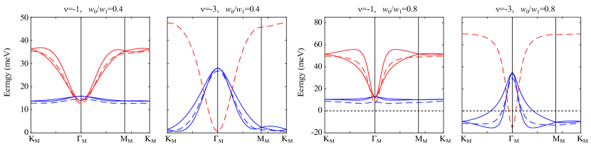
Figure 11: Approximate charge $+1$ (blue) and $-1$ (red) excitations at $\theta=1.05^{\circ}$ at odd fillings in the nonchiral-flat limit. The dashed bands are the excitations in the half-filled valley-spin sectors. The solid blue (red) bands are the +1 ($-1$) excitations in the fully empty (occupied) valley-spin sectors. The flat metric condition is not imposed. In this plot we set the screening length as $\xi=10$nm and accordingly the interaction strength as $U_{\xi}=13$meV. The other parameters are same as in App. A: $v_{F}=5.944{\rm eV\cdot\mathring{A}}$, $|K|=1.703\mathring{\rm A}^{-1}$, $w_{1}=110{\rm meV}$.

F.2 Approximate charge -1 excitations at odd fillings in the nonchiral-flat limit

In the nonchiral-flat limit the states $|\Psi_{\nu}^{\nu_{+},\nu_{-}}\rangle$ at odd fillings $\nu=\pm 1,\pm 3$ are no longer exact eigenstates of the Hamiltonian. However, in Ref. Lian et al. (2020b) we have shown that the states $|\Psi_{-3}^{1,0}\rangle$ (or its U(4) rotations) and $|\Psi_{-1}^{2,1}\rangle$ (or its U(4) rotations) are the lowest states at fillings $\nu=-3,-1$ to first order perturbation of the (first) chiral symmetry breaking. Using the same method as in Section F.1, in this subsection, we derive the approximate charge -1 excitations above these perturbative lowest states.

For the same reason in Section F.1, the spectrum of excitation is given by the eigenvalues of $[H_{I}-\mu N,d_{\mathbf{k},e_{Y},\eta,s}]$. Following the calculation in Section F.1, we have

$$[H_{I}-\mu N,d_{\mathbf{k},e_{Y},\eta,s}]|\Psi_{\nu}^{\nu_{+},\nu_{-}}\rangle=\frac{1}{2\Omega_{tot}}\sum_{\mathbf{q},\mathbf{G},e_{Y}^{\prime}}\bigg{(}V(\mathbf{q}+\mathbf{G})P_{e_{Y}^{\prime},e_{Y}}^{\eta*}(\mathbf{k},\mathbf{q}+\mathbf{G})d_{\mathbf{k},e_{Y}^{\prime},\eta,s}$$

$$\qquad-2\sqrt{V(\mathbf{G}+\mathbf{q})}M_{e_{Y}^{\prime},e_{Y}}^{(\eta)*}\left(\mathbf{k},\mathbf{q}+\mathbf{G}\right)d_{\mathbf{k+q},e_{Y}^{\prime},\eta,s}O_{\mathbf{q,G}}\bigg{)}|\Psi_{\nu}^{\nu_{+},\nu_{-}}\rangle+\mu d_{\mathbf{k},e_{Y},\eta,s}|\Psi_{\nu}^{\nu_{+},\nu_{-}}\rangle,$$ (156)

where $P^{\eta}$ is defined in Eq. 149. When the (first) chiral symmetry is broken, the term $d_{\mathbf{k+q},e_{Y}^{\prime},\eta,s}O_{\mathbf{q,G}}|\Psi_{\nu}^{\nu_{+},\nu_{-}}\rangle$ yields excitations with two holes plus one particle

$$d_{\mathbf{k+q},e_{Y}^{\prime},\eta,s}O_{\mathbf{q,G}}|\Psi_{\nu}^{\nu_{+},\nu_{-}}\rangle=d_{\mathbf{k+q},e_{Y}^{\prime},\eta,s}(O^{0}_{\mathbf{q,G}}+O^{1}_{\mathbf{q,G}})|\Psi_{\nu}^{\nu_{+},\nu_{-}}\rangle$$

$$= \delta_{\mathbf{q},0}A_{\mathbf{G}}N_{M}d_{\mathbf{k},e_{Y}^{\prime},\eta,s}|\Psi_{\nu}^{\nu_{+},\nu_{-}}\rangle+\sum_{\mathbf{k}^{\prime},e_{Y}^{\prime\prime},\eta^{\prime},s^{\prime}}\sqrt{V(\mathbf{q}+\mathbf{G})}\eta^{\prime}F_{e_{Y}^{\prime\prime}}(\mathbf{k}^{\prime},\mathbf{q}+\mathbf{G})d_{\mathbf{k+q},e_{Y}^{\prime},\eta,s}d_{\mathbf{k}^{\prime}+\mathbf{q},-e_{Y}^{\prime\prime},\eta^{\prime},s^{\prime}}^{\dagger}d_{\mathbf{k}^{\prime},e_{Y}^{\prime\prime},\eta^{\prime},s^{\prime}}|\Psi_{\nu}^{\nu_{+},\nu_{-}}\rangle$$ (157)

We now approximate the right hand side by projecting it into the one hole Hilbert space: We only keep the term satisfying $\mathbf{k}^{\prime}=\mathbf{k}$, $e_{Y}^{\prime\prime}=-e_{Y}^{\prime}$, $\eta^{\prime}=\eta$, $s^{\prime}=s$

$$d_{\mathbf{k+q},e_{Y}^{\prime},\eta,s}O_{\mathbf{q,G}}|\Psi_{\nu}^{\nu_{+},\nu_{-}}\rangle=d_{\mathbf{k+q},e_{Y}^{\prime},\eta,s}(O^{0}_{\mathbf{q,G}}+O^{1}_{\mathbf{q,G}})|\Psi_{\nu}^{\nu_{+},\nu_{-}}\rangle$$

$$= \delta_{\mathbf{q},0}A_{\mathbf{G}}N_{M}d_{\mathbf{k},e_{Y}^{\prime},\eta,s}|\Psi_{\nu}^{\nu_{+},\nu_{-}}\rangle+\sqrt{V(\mathbf{q}+\mathbf{G})}\eta F_{-e_{Y}^{\prime}}(\mathbf{k},\mathbf{q}+\mathbf{G})(1-n_{e_{Y}^{\prime},\eta,s})d_{\mathbf{k},-e_{Y}^{\prime},\eta,s}|\Psi_{\nu}^{\nu_{+},\nu_{-}}\rangle\ ,$$ (158)

where $n_{e_{Y}^{\prime},\eta,s}$ equals to 1 if the flavor $\{e_{Y}^{\prime},\eta,s\}$ is occupied and equals to 0 otherwise. If $e_{Y}^{\prime}$ in the second term equals to $e_{Y}$, then there must be $n_{e_{Y}^{\prime},\eta,s}=1$ because we require $\{e_{Y},\eta,s\}$ to be occupied such that $d_{\mathbf{k},e_{Y},\eta,s}|\Psi_{\nu}^{\nu_{+},\nu_{-}}\rangle$ is non-vanishing. Hence we only need to keep the $e_{Y}^{\prime}=-e_{Y}$ in the second term. Then we can rewrite the second term in Eq. 156 as

$$\sum_{e_{Y}^{\prime}}M_{e_{Y}^{\prime},e_{Y}}^{(\eta)*}(\mathbf{k},\mathbf{q}+\mathbf{G})d_{\mathbf{k+q},e_{Y}^{\prime},\eta,s}O_{\mathbf{q,G}}\bigg{)}|\Psi_{\nu}^{\nu_{+},\nu_{-}}\rangle$$

$$= \sum_{e_{Y}^{\prime}}\delta_{\mathbf{q},0}A_{\mathbf{G}}N_{M}M_{e_{Y}^{\prime},e_{Y}}^{(\eta)*}(\mathbf{k},\mathbf{G})d_{\mathbf{k},e_{Y}^{\prime},\eta,s}|\Psi_{\nu}^{\nu_{+},\nu_{-}}\rangle+(1-n_{-e_{Y},\eta,s})\sqrt{V(\mathbf{q}+\mathbf{G})}|F_{e_{Y}}(\mathbf{k},\mathbf{q}+\mathbf{G})|^{2}d_{\mathbf{k},e_{Y},\eta,s}|\Psi_{\nu}^{\nu_{+},\nu_{-}}\rangle\ .$$ (159)

Here we have made use of Eqs. 62 and 53. With the above approximation, we can write the excitation equation as

$$[H_{I}-\mu N,d_{\mathbf{k},e_{Y},\eta,s}]|\Psi_{\nu}^{\nu_{+},\nu_{-}}\rangle\approx\sum_{e_{Y}^{\prime}}\widetilde{R}^{\eta,s}_{e_{Y}^{\prime},e_{Y}}d_{\mathbf{k},e_{Y}^{\prime},\eta,s}|\Psi_{\nu}^{\nu_{+},\nu_{-}}\rangle,$$ (160)

where

$$\widetilde{R}^{\eta,s}_{e_{Y}^{\prime},e_{Y}}= \frac{1}{2\Omega_{\rm tot}}\sum_{\mathbf{q},\mathbf{G}}\bigg{(}V(\mathbf{q}+\mathbf{G})P_{e_{Y}^{\prime},e_{Y}}^{\eta*}(\mathbf{k},\mathbf{q}+\mathbf{G})-2\delta_{\mathbf{q},0}\sqrt{V(\mathbf{G})}A_{\mathbf{G}}N_{M}M_{e_{Y}^{\prime},e_{Y}}^{(\eta)*}\left(\mathbf{k},\mathbf{G}\right)$$

$$-2\delta_{e_{Y}^{\prime},e_{Y}}(1-n_{-e_{Y},\eta,s})V(\mathbf{q}+\mathbf{G})|F_{e_{Y}}(\mathbf{k},\mathbf{q}+\mathbf{G})|^{2}\bigg{)}+\mu\delta_{e_{Y}^{\prime},e_{Y}}.$$ (161)

Notice that both $e_{Y}$ and $e_{Y}^{\prime}$ are limited to fully filled Chern bands in the valley-spin flavor $\eta,s$.

Let us first consider the charge -1 excitation at $\nu=-3$. Without loss of generality, we assume the occupied flavor is $\{+1,\uparrow,+1\}$. For the excitation in the half-filled valley-spin sector ($\{+1,\uparrow\}$), the $e_{Y}$ and $e_{Y}^{\prime}$ indices in $\widetilde{R}^{\eta,s}_{e_{Y}^{\prime},e_{Y}}$ are limited for the occupied Chern band ($+1$). In this case the $\widetilde{R}$ matrix is one-by-one with $n_{-e_{Y},\eta,s}=0$. And there is no hole excitation in the other (fully empty) valley-spin sectors. The calculation for $\nu=-1$ is similar. Due to Ref. Lian et al. (2020b), the perturbative ground state in the nonchiral-flat limit at $\nu=-1$ is $|\Psi_{-1}^{2,1}\rangle$ (or its U(4) rotations). There is a fully occupied valley-spin sector and a half-filled valley-spin sector. In the half-filled valley-spin sector $\widetilde{R}$ is one-by-one with $n_{-e_{Y},\eta,s}=0$ and in the fully occupied valley-spin sector $\widetilde{R}$ is two-by-two with $n_{-e_{Y},\eta,s}=1$. The approximate charge $-1$ excitations are shown in Fig. 11.

F.3 Approximate charge neutral excitations at odd fillings in the nonchiral-flat U(4) limit

In the nonchiral-flat limit the states $|\Psi_{\nu}^{\nu_{+},\nu_{-}}\rangle$ at odd fillings $\nu=\pm 1,\pm 3$ are no longer exact eigenstates of the Hamiltonian. However, in Ref. Lian et al. (2020b) we have shown that the states $|\Psi_{-3}^{1,0}\rangle$ (or its U(4) rotations) and $|\Psi_{-1}^{2,1}\rangle$ (or its U(4) rotations) are the lowest states at fillings $\nu=-3,-1$ to first order perturbation of the (first) chiral symmetry breaking. In this subsection, we derive the approximate charge neutral excitations above these perturbative lowest states.

Since these states have fully occupied Chern bands, it is convenient to work in the Chern band basis. Following the calculations in Section D.1, we have

$$[H_{I}-\mu N,d_{\mathbf{k}+\mathbf{p},e_{Y2},\eta_{2},s_{2}}^{\dagger}d_{\mathbf{k},e_{Y1},\eta_{1},s_{1}}]|\Psi_{\nu}^{\nu_{+},\nu_{-}}\rangle$$

$$= \frac{1}{2\Omega_{\rm tot}}\sum_{\mathbf{q},\mathbf{G}}\bigg{(}\sum_{e_{Y}}P^{\eta_{2}}_{e_{Y},e_{Y2}}(\mathbf{k}+\mathbf{p},\mathbf{q}+\mathbf{G})d_{\mathbf{k}+\mathbf{p},e_{Y},\eta_{2},s_{2}}^{\dagger}d_{\mathbf{k},e_{Y1},\eta_{1},s_{1}}+\sum_{e_{Y}^{\prime}}P_{e_{Y}^{\prime},e_{Y1}}^{\eta_{1}*}(\mathbf{k},\mathbf{q}+\mathbf{G})d_{\mathbf{k}+\mathbf{p},e_{Y2},\eta_{2},s_{2}}^{\dagger}d_{\mathbf{k},e_{Y}^{\prime},\eta_{1},s_{1}}$$

$$+2\sqrt{V(\mathbf{G}+\mathbf{q})}\sum_{e_{Y}}M_{e_{Y},e_{Y2}}^{\left(\eta_{2}\right)}\left(\mathbf{k}+\mathbf{p},\mathbf{q}+\mathbf{G}\right)d_{\mathbf{k}+\mathbf{p}+\mathbf{q},e_{Y},\eta_{2},s_{2}}^{\dagger}d_{\mathbf{k},e_{Y1},\eta_{1},s_{1}}O_{-\mathbf{q,-G}}$$

$$-2\sqrt{V(\mathbf{G}+\mathbf{q})}\sum_{e_{Y}^{\prime}}M_{e_{Y}^{\prime},e_{Y1}}^{\left(\eta_{1}\right)*}\left(\mathbf{k},-\mathbf{q}-\mathbf{G}\right)d_{\mathbf{k}+\mathbf{p},e_{Y2},\eta_{2},s_{2}}^{\dagger}d_{\mathbf{k}-\mathbf{q},e_{Y}^{\prime},\eta_{1},s_{1}}O_{-\mathbf{q,-G}}$$

$$-2V(\mathbf{G}+\mathbf{q})\sum_{e_{Y},e_{Y}^{\prime}}M_{e_{Y},e_{Y2}}^{\left(\eta_{2}\right)}\left(\mathbf{k}+\mathbf{p},\mathbf{q}+\mathbf{G}\right)M_{e_{Y}^{\prime},e_{Y1}}^{\left(\eta_{1}\right)*}\left(\mathbf{k},\mathbf{q}+\mathbf{G}\right)d_{\mathbf{k}+\mathbf{p}+\mathbf{q},e_{Y},\eta_{2},s_{2}}^{\dagger}d_{\mathbf{k}+\mathbf{q},e_{Y}^{\prime},\eta_{1},s_{1}}\bigg{)}|\Psi_{\nu}^{\nu_{+},\nu_{-}}\rangle\ .$$ (162)

In the (first) chiral limit, where $O_{-\mathbf{q},-\mathbf{G}}|\Psi_{\nu}^{\nu_{+},\nu_{-}}\rangle=\delta_{\mathbf{q},0}A_{-\mathbf{G}}N_{M}|\Psi_{\nu}^{\nu_{+},\nu_{-}}\rangle$, the right hand side of the above equation only involve excitations with one pair of particle and hole. However, when the (first) chiral symmetry is broken, $O_{-\mathbf{q},-\mathbf{G}}|\Psi_{\nu}^{\nu_{+},\nu_{-}}\rangle$ will yield additional particle-hole excitations:

$$d_{\mathbf{k}+\mathbf{p}+\mathbf{q},e_{Y},\eta_{2},s_{2}}^{\dagger}d_{\mathbf{k},e_{Y1},\eta_{1},s_{1}}O_{-\mathbf{q,-G}}|\Psi_{\nu}^{\nu_{+},\nu_{-}}\rangle=d_{\mathbf{k}+\mathbf{p}+\mathbf{q},e_{Y},\eta_{2},s_{2}}^{\dagger}d_{\mathbf{k},m_{1},\eta_{1},s_{1}}(O^{0}_{-\mathbf{q},-\mathbf{G}}+O^{1}_{-\mathbf{q},-\mathbf{G}})|\Psi_{\nu}^{\nu_{+},\nu_{-}}\rangle$$

$$= \delta_{\mathbf{q},0}A_{-\mathbf{G}}N_{M}d_{\mathbf{k}+\mathbf{p},e_{Y},\eta_{2},s_{2}}^{\dagger}d_{\mathbf{k},e_{Y1},\eta_{1},s_{1}}|\Psi_{\nu}^{\nu_{+},\nu_{-}}\rangle+\sum_{\mathbf{k}^{\prime\prime},e_{Y}^{\prime\prime},\eta^{\prime\prime},s^{\prime\prime}}\sqrt{V(\mathbf{q}+\mathbf{G})}\eta^{\prime\prime}F_{e_{Y}^{\prime\prime}}(\mathbf{k}^{\prime\prime},-\mathbf{q}-\mathbf{G})$$

$$\qquad\times d_{\mathbf{k}+\mathbf{p}+\mathbf{q},e_{Y},\eta_{2},s_{2}}^{\dagger}d_{\mathbf{k},e_{Y1},\eta_{1},s_{1}}d_{\mathbf{k}^{\prime\prime}-\mathbf{q},-e_{Y}^{\prime\prime},\eta^{\prime\prime},s^{\prime\prime}}^{\dagger}d_{\mathbf{k}^{\prime\prime},e_{Y}^{\prime\prime},\eta^{\prime\prime},s^{\prime\prime}}|\Psi_{\nu}^{\nu_{+},\nu_{-}}\rangle\ .$$ (163)

We approximate the above equation by projecting it into the Hilbert space of excitations with only one pair of particle and hole. According to the Wick’s theorem, we have

$$d_{\mathbf{k}+\mathbf{p}+\mathbf{q},e_{Y},\eta_{2},s_{2}}^{\dagger}d_{\mathbf{k},e_{Y1},\eta_{1},s_{1}}d_{\mathbf{k}^{\prime\prime}-\mathbf{q},-e_{Y}^{\prime\prime},\eta^{\prime\prime},s^{\prime\prime}}^{\dagger}d_{\mathbf{k}^{\prime\prime},e_{Y}^{\prime\prime},\eta^{\prime\prime},s^{\prime\prime}}=:d_{\mathbf{k}+\mathbf{p}+\mathbf{q},e_{Y},\eta_{2},s_{2}}^{\dagger}d_{\mathbf{k},e_{Y1},\eta_{1},s_{1}}d_{\mathbf{k}^{\prime\prime}-\mathbf{q},-e_{Y}^{\prime\prime},\eta^{\prime\prime},s^{\prime\prime}}^{\dagger}d_{\mathbf{k}^{\prime\prime},e_{Y}^{\prime\prime},\eta^{\prime\prime},s^{\prime\prime}}:$$

$$+\langle\Psi_{\nu}^{\nu_{+},\nu_{-}}|d_{\mathbf{k}+\mathbf{p}+\mathbf{q},e_{Y},\eta_{2},s_{2}}^{\dagger}d_{\mathbf{k},e_{Y1},\eta_{1},s_{1}}|\Psi_{\nu}^{\nu_{+},\nu_{-}}\rangle d_{\mathbf{k}^{\prime\prime}-\mathbf{q},-e_{Y}^{\prime\prime},\eta^{\prime\prime},s^{\prime\prime}}^{\dagger}d_{\mathbf{k}^{\prime\prime},e_{Y}^{\prime\prime},\eta^{\prime\prime},s^{\prime\prime}}$$

$$+\langle\Psi_{\nu}^{\nu_{+},\nu_{-}}|d_{\mathbf{k}+\mathbf{p}+\mathbf{q},e_{Y},\eta_{2},s_{2}}^{\dagger}d_{\mathbf{k}^{\prime\prime},e_{Y}^{\prime\prime},\eta^{\prime\prime},s^{\prime\prime}}|\Psi_{\nu}^{\nu_{+},\nu_{-}}\rangle d_{\mathbf{k},e_{Y1},\eta_{1},s_{1}}d_{\mathbf{k}^{\prime\prime}-\mathbf{q},-e_{Y}^{\prime\prime},\eta^{\prime\prime},s^{\prime\prime}}^{\dagger}$$

$$+\langle\Psi_{\nu}^{\nu_{+},\nu_{-}}|d_{\mathbf{k},e_{Y1},\eta_{1},s_{1}}d_{\mathbf{k}^{\prime\prime}-\mathbf{q},-e_{Y}^{\prime\prime},\eta^{\prime\prime},s^{\prime\prime}}^{\dagger}|\Psi_{\nu}^{\nu_{+},\nu_{-}}\rangle d_{\mathbf{k}+\mathbf{p}+\mathbf{q},e_{Y},\eta_{2},s_{2}}^{\dagger}d_{\mathbf{k}^{\prime\prime},e_{Y}^{\prime\prime},\eta^{\prime\prime},s^{\prime\prime}}$$

$$-\langle\Psi_{\nu}^{\nu_{+},\nu_{-}}|d_{\mathbf{k},e_{Y1},\eta_{1},s_{1}}d_{\mathbf{k}^{\prime\prime}-\mathbf{q},-e_{Y}^{\prime\prime},\eta^{\prime\prime},s^{\prime\prime}}^{\dagger}|\Psi_{\nu}^{\nu_{+},\nu_{-}}\rangle\langle\Psi_{\nu}^{\nu_{+},\nu_{-}}|d_{\mathbf{k}+\mathbf{p}+\mathbf{q},e_{Y},\eta_{2},s_{2}}^{\dagger}d_{\mathbf{k}^{\prime\prime},e_{Y}^{\prime\prime},\eta^{\prime\prime},s^{\prime\prime}}|\Psi_{\nu}^{\nu_{+},\nu_{-}}\rangle$$ (164)

Here $:A:$ represents the normal ordered form of the operator $A$ with respect to $|\Psi_{\nu}^{\nu_{+},\nu_{-}}\rangle$, where all the creation operators of occupied states and annihilation operators of empty states are on the right hand side of the creation operators of empty states and annihilation operators of occupied states. The first (normal ordered) term is non-vanishing when acted on $|\Psi_{\nu}^{\nu_{+},\nu_{-}}\rangle$ if the two creation operators are of empty states and the two annihilation operators are of occupied states. However, we will omit this term because it yields two particle-hole pairs. Since we require $d_{\mathbf{k},e_{Y1},\eta_{1},s_{1}}$ to be occupied such that the initial state is non-vanishing, there must be $\langle\Psi_{\nu}^{\nu_{+},\nu_{-}}|d_{\mathbf{k},e_{Y1},\eta_{1},s_{1}}=0$ and hence the last two terms in the above equation vanish. Then we obtain

$$d_{\mathbf{k}+\mathbf{p}+\mathbf{q},e_{Y},\eta_{2},s_{2}}^{\dagger}d_{\mathbf{k},e_{Y1},\eta_{1},s_{1}}d_{\mathbf{k}^{\prime\prime}-\mathbf{q},-e_{Y}^{\prime\prime},\eta^{\prime\prime},s^{\prime\prime}}^{\dagger}d_{\mathbf{k}^{\prime\prime},e_{Y}^{\prime\prime},\eta^{\prime\prime},s^{\prime\prime}}$$

$$\approx \delta_{\mathbf{p}+\mathbf{q},0}\delta_{e_{Y},e_{Y1}}\delta_{\eta_{2},\eta_{1}}\delta_{s_{2},s_{1}}d_{\mathbf{k}^{\prime\prime}-\mathbf{q},-e_{Y}^{\prime\prime},\eta^{\prime\prime},s^{\prime\prime}}^{\dagger}d_{\mathbf{k}^{\prime\prime},e_{Y}^{\prime\prime},\eta^{\prime\prime},s^{\prime\prime}}$$

$$-\delta_{\mathbf{k}+\mathbf{p}+\mathbf{q},\mathbf{k}^{\prime\prime}}\delta_{e_{Y},e_{Y}^{\prime\prime}}\delta_{\eta_{2},\eta^{\prime\prime}}\delta_{s_{2},s^{\prime\prime}}n_{e_{Y},\eta_{2},s_{2}}d_{\mathbf{k}+\mathbf{p},-e_{Y},\eta,s}^{\dagger}d_{\mathbf{k},e_{Y1},\eta_{1},s_{1}}\ ,$$ (165)

where $n_{e_{Y},\eta,s}$ equals to 1 if the flavor $\{e_{Y},\eta,s\}$ is occupied and equals to 0 otherwise. Here we have made use of $\{d_{\mathbf{k}+\mathbf{p},-e_{Y},\eta,s}^{\dagger},d_{\mathbf{k},e_{Y1},\eta_{1},s_{1}}\}=0$, which is because $\{e_{Y1},\eta_{1},s_{1}\}$ is required to be occupied and $\{-e_{Y},\eta,s\}$ is required to be empty and hence $\{e_{Y1},\eta_{1},s_{1}\}\neq\{-e_{Y},\eta,s\}$. Then we obtain

$$d_{\mathbf{k}+\mathbf{p}+\mathbf{q},e_{Y},\eta_{2},s_{2}}^{\dagger}d_{\mathbf{k},e_{Y1},\eta_{1},s_{1}}O_{-\mathbf{q,-G}}|\Psi_{\nu}^{\nu_{+},\nu_{-}}\rangle\approx\delta_{\mathbf{q},0}A_{-\mathbf{G}}N_{M}d_{\mathbf{k}+\mathbf{p},e_{Y},\eta_{2},s_{2}}^{\dagger}d_{\mathbf{k},e_{Y1},\eta_{1},s_{1}}|\Psi_{\nu}^{\nu_{+},\nu_{-}}\rangle$$

$$-\sqrt{V(\mathbf{q}+\mathbf{G})}\eta_{2}F_{e_{Y}}(\mathbf{k}+\mathbf{p}+\mathbf{q},-\mathbf{q}-\mathbf{G})n_{e_{Y},\eta_{2},s_{2}}d_{\mathbf{k}+\mathbf{p},-e_{Y},\eta,s}^{\dagger}d_{\mathbf{k},e_{Y1},\eta_{1},s_{1}}$$

$$+\delta_{\mathbf{p}+\mathbf{q},0}\delta_{e_{Y},e_{Y1}}\delta_{\eta_{2},\eta_{1}}\delta_{s_{2},s_{1}}\sum_{\mathbf{k}^{\prime\prime},e_{Y}^{\prime\prime},\eta^{\prime\prime},s^{\prime\prime}}\sqrt{V(\mathbf{q}+\mathbf{G})}\eta^{\prime\prime}F_{e_{Y}^{\prime\prime}}(\mathbf{k}^{\prime\prime},-\mathbf{q}-\mathbf{G})d_{\mathbf{k}^{\prime\prime}-\mathbf{q},-e_{Y}^{\prime\prime},\eta^{\prime\prime},s^{\prime\prime}}^{\dagger}d_{\mathbf{k}^{\prime\prime},e_{Y}^{\prime\prime},\eta^{\prime\prime},s^{\prime\prime}}\ .$$ (166)

Similarly, we have

$$d_{\mathbf{k}+\mathbf{p},e_{Y2},\eta_{2},s_{2}}^{\dagger}d_{\mathbf{k}-\mathbf{q},e_{Y}^{\prime},\eta_{1},s_{1}}d_{\mathbf{k}^{\prime\prime}-\mathbf{q},-e_{Y}^{\prime\prime},\eta^{\prime\prime},s^{\prime\prime}}^{\dagger}d_{\mathbf{k}^{\prime\prime},e_{Y}^{\prime\prime},\eta^{\prime\prime},s^{\prime\prime}}$$

$$\approx \langle\Psi_{\nu}^{\nu_{+},\nu_{-}}|d_{\mathbf{k}+\mathbf{p},e_{Y2},\eta_{2},s_{2}}^{\dagger}d_{\mathbf{k}-\mathbf{q},e_{Y}^{\prime},\eta_{1},s_{1}}|\Psi_{\nu}^{\nu_{+},\nu_{-}}\rangle d_{\mathbf{k}^{\prime\prime}-\mathbf{q},-e_{Y}^{\prime\prime},\eta^{\prime\prime},s^{\prime\prime}}^{\dagger}d_{\mathbf{k}^{\prime\prime},e_{Y}^{\prime\prime},\eta^{\prime\prime},s^{\prime\prime}}$$

$$+\langle\Psi_{\nu}^{\nu_{+},\nu_{-}}|d_{\mathbf{k}+\mathbf{p},e_{Y2},\eta_{2},s_{2}}^{\dagger}d_{\mathbf{k}^{\prime\prime},e_{Y}^{\prime\prime},\eta^{\prime\prime},s^{\prime\prime}}|\Psi_{\nu}^{\nu_{+},\nu_{-}}\rangle d_{\mathbf{k}-\mathbf{q},e_{Y}^{\prime},\eta_{1},s_{1}}d_{\mathbf{k}^{\prime\prime}-\mathbf{q},-e_{Y}^{\prime\prime},\eta^{\prime\prime},s^{\prime\prime}}^{\dagger}$$

$$+\langle\Psi_{\nu}^{\nu_{+},\nu_{-}}|d_{\mathbf{k}-\mathbf{q},e_{Y}^{\prime},\eta_{1},s_{1}}d_{\mathbf{k}^{\prime\prime}-\mathbf{q},-e_{Y}^{\prime\prime},\eta^{\prime\prime},s^{\prime\prime}}^{\dagger}|\Psi_{\nu}^{\nu_{+},\nu_{-}}\rangle d_{\mathbf{k}+\mathbf{p},e_{Y2},\eta_{2},s_{2}}^{\dagger}d_{\mathbf{k}^{\prime\prime},e_{Y}^{\prime\prime},\eta^{\prime\prime},s^{\prime\prime}}$$

$$-\langle\Psi_{\nu}^{\nu_{+},\nu_{-}}|d_{\mathbf{k}-\mathbf{q},e_{Y}^{\prime},\eta_{1},s_{1}}d_{\mathbf{k}^{\prime\prime}-\mathbf{q},-e_{Y}^{\prime\prime},\eta^{\prime\prime},s^{\prime\prime}}^{\dagger}|\Psi_{\nu}^{\nu_{+},\nu_{-}}\rangle\langle\Psi_{\nu}^{\nu_{+},\nu_{-}}|d_{\mathbf{k}+\mathbf{p},e_{Y2},\eta_{2},s_{2}}^{\dagger}d_{\mathbf{k}^{\prime\prime},e_{Y}^{\prime\prime},\eta^{\prime\prime},s^{\prime\prime}}|\Psi_{\nu}^{\nu_{+},\nu_{-}}\rangle.$$

$$\approx \delta_{\mathbf{k},\mathbf{k}^{\prime\prime}}\delta_{e_{Y}^{\prime},-e_{Y}^{\prime\prime}}\delta_{\eta_{1},\eta^{\prime\prime}}\delta_{s_{1},s^{\prime\prime}}(1-n_{e_{Y}^{\prime},\eta_{1},s_{1}})d_{\mathbf{k}+\mathbf{p},e_{Y2},\eta_{2},s_{2}}^{\dagger}d_{\mathbf{k}^{\prime\prime},e_{Y}^{\prime\prime},\eta^{\prime\prime},s^{\prime\prime}},$$ (167)

where we have made use of $\langle\Psi_{\nu}^{\nu_{+},\nu_{-}}|d_{\mathbf{k}+\mathbf{p},e_{Y2},\eta_{2},s_{2}}^{\dagger}=0$, and hence

$$d_{\mathbf{k}+\mathbf{p},e_{Y2},\eta_{2},s_{2}}^{\dagger}d_{\mathbf{k}-\mathbf{q},e_{Y}^{\prime},\eta_{1},s_{1}}O_{-\mathbf{q,-G}}|\Psi_{\nu}^{\nu_{+},\nu_{-}}\rangle\approx\delta_{\mathbf{q},0}A_{-\mathbf{G}}N_{M}d_{\mathbf{k}+\mathbf{p},e_{Y},\eta_{2},s_{2}}^{\dagger}d_{\mathbf{k},e_{Y1},\eta_{1},s_{1}}|\Psi_{\nu}^{\nu_{+},\nu_{-}}\rangle$$

$$+\sqrt{V(\mathbf{q}+\mathbf{G})}\eta_{1}F_{-e_{Y1}}(\mathbf{k},-\mathbf{q}-\mathbf{G})(1-n_{e_{Y}^{\prime},\eta_{1},s_{1}})d_{\mathbf{k}+\mathbf{p},e_{Y2},\eta,s}^{\dagger}d_{\mathbf{k},-e_{Y}^{\prime},\eta_{1},s_{1}}\ .$$ (168)

Substituting Sections F.3 and F.3 into Section F.3, we obtain

$$[H_{I}-\mu N,d_{\mathbf{k}+\mathbf{p},e_{Y2},\eta_{2},s_{2}}^{\dagger}d_{\mathbf{k},e_{Y1},\eta_{1},s_{1}}]|\Psi_{\nu}^{\nu_{+},\nu_{-}}\rangle$$

$$\approx \bigg{(}\sum_{e_{Y}}R^{\eta_{2},s_{2}}_{e_{Y},e_{Y2}}(\mathbf{k}+\mathbf{p})d_{\mathbf{k}+\mathbf{p},e_{Y},\eta_{2},s_{2}}^{\dagger}d_{\mathbf{k},e_{Y1},\eta_{1},s_{1}}+\sum_{e_{Y}^{\prime}}\widetilde{R}_{e_{Y}^{\prime},e_{Y1}}^{\eta_{1},s_{1}*}(\mathbf{k})d_{\mathbf{k}+\mathbf{p},e_{Y2},\eta_{2},s_{2}}^{\dagger}d_{\mathbf{k},e_{Y}^{\prime},\eta_{1},s_{1}}\bigg{)}|\Psi_{\nu}^{\nu_{+},\nu_{-}}\rangle$$

$$-\frac{1}{\Omega_{\rm tot}}\sum_{\mathbf{q},\mathbf{G}}V(\mathbf{G}+\mathbf{q})\sum_{e_{Y},e_{Y}^{\prime}}M_{e_{Y},e_{Y2}}^{\left(\eta_{2}\right)}\left(\mathbf{k}+\mathbf{p},\mathbf{q}+\mathbf{G}\right)M_{e_{Y}^{\prime},e_{Y1}}^{\left(\eta_{1}\right)*}\left(\mathbf{k},\mathbf{q}+\mathbf{G}\right)d_{\mathbf{k}+\mathbf{p}+\mathbf{q},e_{Y},\eta_{2},s_{2}}^{\dagger}d_{\mathbf{k}+\mathbf{q},e_{Y}^{\prime},\eta_{1},s_{1}}|\Psi_{\nu}^{\nu_{+},\nu_{-}}\rangle$$

$$+\frac{\delta_{\eta_{2}\eta_{1}}\delta_{s_{2},s_{1}}}{\Omega_{\rm tot}}\sum_{\mathbf{G}}\sum_{\mathbf{k}^{\prime\prime}e_{Y}^{\prime\prime}\eta^{\prime\prime}s^{\prime\prime}}V(-\mathbf{p}+\mathbf{G})M^{(\eta_{2})}_{e_{Y1},e_{Y2}}(\mathbf{k}+\mathbf{p},-\mathbf{p}+\mathbf{G})\eta^{\prime\prime}F_{e_{Y}^{\prime\prime}}(\mathbf{k}^{\prime\prime},\mathbf{p}-\mathbf{G})d_{\mathbf{k}^{\prime\prime}+\mathbf{p},-e_{Y}^{\prime\prime},\eta^{\prime\prime},s^{\prime\prime}}^{\dagger}d_{\mathbf{k}^{\prime\prime},e_{Y}^{\prime\prime},\eta^{\prime\prime},s^{\prime\prime}}|\Psi_{\nu}^{\nu_{+},\nu_{-}}\rangle\ ,$$ (169)

where $R^{\eta_{2},s_{2}}$ and $\widetilde{R}^{\eta_{1},s_{1}}$ are given by Eqs. 155 and F.2, respectively. The last term is nonzero only if $\{e_{Y1},\eta_{1},s_{1}\}$ is occupied and $\{e_{Y2},\eta_{2},s_{2}\}$ is empty, which, provided $\eta_{2}=\eta_{1}$ and $s_{2}=s_{1}$, also implies $e_{Y1}$ must equal to $-e_{Y2}$. Thus we can rewrite the last term as

$$\frac{\delta_{e_{Y2},-e_{Y1}}\delta_{\eta_{2}\eta_{1}}\delta_{s_{2},s_{1}}}{\Omega_{\rm tot}}\sum_{\mathbf{G}}\sum_{\mathbf{k}^{\prime\prime}e_{Y}\eta s}{V(-\mathbf{p}+\mathbf{G})}\eta_{2}F_{e_{Y2}}(\mathbf{k}+\mathbf{p},-\mathbf{p}+\mathbf{G})\eta F_{-e_{Y}}(\mathbf{k}^{\prime\prime},\mathbf{p}-\mathbf{G})d_{\mathbf{k}^{\prime\prime}+\mathbf{p},e_{Y},\eta,s}^{\dagger}d_{\mathbf{k}^{\prime\prime},-e_{Y},\eta,s}|\Psi_{\nu}^{\nu_{+},\nu_{-}}\rangle$$

$$= \frac{\delta_{e_{Y2},-e_{Y1}}\delta_{\eta_{2}\eta_{1}}\delta_{s_{2},s_{1}}}{\Omega_{\rm tot}}\sum_{\mathbf{G}}\sum_{\mathbf{k}^{\prime\prime}e_{Y}\eta s}{V(-\mathbf{p}+\mathbf{G})}\eta_{2}F_{e_{Y2}}(\mathbf{k},\mathbf{p}-\mathbf{G})\eta F_{e_{Y}}^{*}(\mathbf{k}^{\prime\prime},\mathbf{p}-\mathbf{G})d_{\mathbf{k}^{\prime\prime}+\mathbf{p},e_{Y},\eta,s}^{\dagger}d_{\mathbf{k}^{\prime\prime},-e_{Y},\eta,s}|\Psi_{\nu}^{\nu_{+},\nu_{-}}\rangle\ ,$$ (170)

where we have made use of Eqs. 62 and 53. Therefore, we can write the scattering equation as

$$[H_{I}-\mu N,d_{\mathbf{k}+\mathbf{p},e_{Y2},\eta_{2},s_{2}}^{\dagger}d_{\mathbf{k},e_{Y1},\eta_{1},s_{1}}]|\Psi_{\nu}^{\nu_{+},\nu_{-}}\rangle$$

$$\approx \sum_{\eta,s,\eta^{\prime},s^{\prime}}\sum_{e_{Y},e_{Y}^{\prime}}\sum_{\mathbf{q}}S^{\eta,s,\eta^{\prime},s^{\prime};\eta_{2},s_{2},\eta_{1},s_{1}}_{e_{Y},e_{Y}^{\prime};e_{Y2},e_{Y1}}(\mathbf{k}+\mathbf{q},\mathbf{k};\mathbf{p})d_{\mathbf{k}+\mathbf{q}+\mathbf{p},e_{Y},\eta,s}^{\dagger}d_{\mathbf{k}+\mathbf{q},e_{Y}^{\prime},\eta^{\prime},s^{\prime}}|\Psi_{\nu}^{\nu_{+},\nu_{-}}\rangle\ ,$$ (171)

where the scattering matrix is

$$S^{\eta,s,\eta^{\prime},s^{\prime};\eta_{2},s_{2},\eta_{1},s_{1}}_{e_{Y},e_{Y}^{\prime};e_{Y2},e_{Y1}}(\mathbf{k}+\mathbf{q},\mathbf{k};\mathbf{p})=\delta_{\eta,\eta_{2}}\delta_{s,s_{2}}\delta_{\eta^{\prime},\eta_{1}}\delta_{s^{\prime},s_{1}}\bigg{(}\delta_{\mathbf{q},0}\Big{(}R^{\eta_{2},s_{2}}_{e_{Y},e_{Y2}}(\mathbf{k}+\mathbf{p})\delta_{e_{Y}^{\prime},e_{Y1}}+\delta_{e_{Y},e_{Y2}}\widetilde{R}^{\eta_{1},s_{1}}_{e_{Y}^{\prime},e_{Y1}}(\mathbf{k})\Big{)}$$

$$\qquad-\frac{1}{\Omega_{\rm tot}}\sum_{\mathbf{G}}V(\mathbf{G}+\mathbf{q})M_{e_{Y},e_{Y2}}^{\left(\eta_{2}\right)}\left(\mathbf{k}+\mathbf{p},\mathbf{q}+\mathbf{G}\right)M_{e_{Y}^{\prime},e_{Y1}}^{\left(\eta_{1}\right)*}\left(\mathbf{k},\mathbf{q}+\mathbf{G}\right)\bigg{)}$$

$$\qquad+\delta_{e_{Y2},-e_{Y1}}\delta_{\eta_{2}\eta_{1}}\delta_{s_{2},s_{1}}\delta_{e_{Y},-e_{Y}^{\prime}}\delta_{\eta\eta^{\prime}}\delta_{ss^{\prime}}\frac{1}{\Omega_{\rm tot}}\sum_{\mathbf{G}}{V(-\mathbf{p}+\mathbf{G})}\eta F_{e_{Y}}^{*}(\mathbf{k}+\mathbf{q},\mathbf{p}-\mathbf{G})\eta_{2}F_{e_{Y2}}(\mathbf{k},\mathbf{p}-\mathbf{G})\ .$$ (172)

The last term is nonzero if both the $\{\eta_{2},s_{2}\}$ and $\{\eta,s\}$ valley-spin flavors are halfly filled. It couples all the halfly filled valley-spin flavors, which are independent in the (first) chiral-flat limit, to each other.

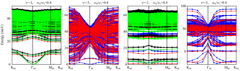
Figure 12: Approximate charge neutral excitations at $\theta=1.05^{\circ}$ at odd fillings in the nonchiral-flat limit. The flat metric condition is not imposed. Blue, red, black, and green bands are in the empty-half, half-half, empty-filled, half-filled sectors, respectively. (See the text for the definition of sectors.) In this plot we set the screening length as $\xi=10$nm and accordingly the interaction strength as $U_{\xi}=13$meV. The other parameters are same as in App. A: $v_{F}=5.944{\rm eV\cdot\mathring{A}}$, $|K|=1.703\mathring{\rm A}^{-1}$, $w_{1}=110{\rm meV}$.

According to Lian et al. (2020b), in the nonchiral-flat limit the state $\Psi_{-3}^{1,0}$ (or its U(4) rotations) is still the perturbative ground state at $\nu=-3$. Without loss of generality, we assume the occupied flavor is $\{+1,\uparrow,+1\}$. Then we can divide the neutral excitations into the following sectors:

1. The half-half sector, where $\eta_{2}=\eta_{1}=+1$, $s_{2}=s_{1}=\uparrow$. The delta functions in the first term of Section F.3 require $\eta=\eta^{\prime}=+1$, $s=s^{\prime}=\uparrow$. The delta functions in the second term requires $\eta=\eta^{\prime}$ and $s=s^{\prime}$. Since $d_{\eta,s,e_{Y}}^{\dagger}$ and $d_{\eta^{\prime},s^{\prime},e_{Y}^{\prime}}$ must belong to empty and occupied bands, there must also be $\eta=\eta^{\prime}=+1$, $s=s^{\prime}=\uparrow$ in the second term. Then it follows that $e_{Y}=e_{Y2}=-1$, $e_{Y}^{\prime}=e_{Y1}=+1$. At given $\mathbf{k},\mathbf{p},\mathbf{q}$, the $S$ matrix is a one-by-one matrix.

2. The empty-half sector, where $\{\eta_{2},s_{2}\}$ is an empty valley-spin sector and $\{\eta_{1},s_{1}\}$ is a half-filled valley-spin sector. The second term of Section F.3 vanish due to the delta function $\delta_{\eta_{2}\eta_{1}}\delta_{s_{2}s_{1}}$. The delta functions in the first term requires $\eta=\eta_{2}$, $s=s_{2}$, $\eta^{\prime}=\eta_{1}$, $s^{\prime}=s_{1}$. It follows that $e_{Y}^{\prime}=e_{Y1}=+1$ and $e_{Y},e_{Y2}$ take values in $\pm 1$. At given $\mathbf{k},\mathbf{p},\mathbf{q}$, the $S$ matrix is a two-by-two matrix.

According to Lian et al. (2020b), in the nonchiral-flat limit the state $\Psi_{-1}^{2,1}$ (or its U(4) rotations) is still the perturbative ground state at $\nu=-1$. There is a fully occupied valley-spin sector and a half filled valley-spin sector. Without loss of generality, we assume the occupied flavors as $\{+1,\uparrow,+1\}$, $\{+1,\uparrow,-1\}$, $\{+1,\downarrow,+1\}$. Then we can divide the neutral excitations into the following sectors:

1. The half-half sector, where $\eta_{2}=\eta_{1}=+1$, $s_{2}=s_{1}=\downarrow$. The delta functions in the first term of Section F.3 require $\eta=\eta^{\prime}=+1$, $s=s^{\prime}=\downarrow$. The delta functions in the second term requires $\eta=\eta^{\prime}$ and $s=s^{\prime}$. Since $d_{\eta,s,e_{Y}}^{\dagger}$ and $d_{\eta^{\prime},s^{\prime},e_{Y}^{\prime}}$ must belong to empty and occupied bands, there must also be $\eta=\eta^{\prime}=+1$, $s=s^{\prime}=\downarrow$ (the half filled valley-spin sector) in the second term. Then it follows that $e_{Y}=e_{Y2}=-1$, $e_{Y}^{\prime}=e_{Y1}=+1$. At given $\mathbf{k},\mathbf{p},\mathbf{q}$, the $S$ matrix is a one-by-one matrix.

2. The empty-half sector, where $\{\eta_{2},s_{2}\}$ is an empty valley-spin sector and $\{\eta_{1},s_{1}\}$ is a half-filled valley-spin sector. The second term of Section F.3 vanish due to the delta function $\delta_{\eta_{2}\eta_{1}}\delta_{s_{2}s_{1}}$. The delta functions in the first term requires $\eta=\eta_{2}$, $s=s_{2}$, $\eta^{\prime}=\eta_{1}$, $s^{\prime}=s_{1}$. It follows that $e_{Y}^{\prime}=e_{Y1}=+1$ and $e_{Y},e_{Y2}$ take values in $\pm 1$. At given $\mathbf{k},\mathbf{p},\mathbf{q}$, the $S$ matrix is a two-by-two matrix.

3. The half-occupied sector, where $\{\eta_{2},s_{2}\}$ is the half filled valley-spin sector $\{+1,\downarrow\}$ and $\{\eta_{1},s_{1}\}$ is the fully occupied valley-spin sector $\{+1,\uparrow\}$. The second term of Section F.3 vanish due to the delta function $\delta_{\eta_{2}\eta_{1}}\delta_{s_{2}s_{1}}$. The delta functions in the first term requires $\eta=\eta_{2}$, $s=s_{2}$, $\eta^{\prime}=\eta_{1}$, $s^{\prime}=s_{1}$. It follows that $e_{Y}^{\prime},e_{Y1}$ take values in $\pm 1$ and $e_{Y}=e_{Y2}=-1$. At given $\mathbf{k},\mathbf{p},\mathbf{q}$, the $S$ matrix is a two-by-two matrix.

4. The empty-occupied sector, where $\{\eta_{2},s_{2}\}$ is an empty valley-spin sector and $\{\eta_{1},s_{1}\}$ is the fully occupied valley-spin sector $\{+1,\uparrow\}$. The second term of Section F.3 vanish due to the delta function $\delta_{\eta_{2}\eta_{1}}\delta_{s_{2}s_{1}}$. The delta functions in the first term requires $\eta=\eta_{2}$, $s=s_{2}$, $\eta^{\prime}=\eta_{1}$, $s^{\prime}=s_{1}$. It follows that $e_{Y}^{\prime},e_{Y1},e_{Y},e_{Y2}$ all take values in $\pm 1$. At given $\mathbf{k},\mathbf{p},\mathbf{q}$, the $S$ matrix is a four-by-four matrix.

The numerical results are shown in Fig. 12.

References

- Bistritzer and MacDonald (2011) Rafi Bistritzer and Allan H. MacDonald, “Moiré bands in twisted double-layer graphene,” Proceedings of the National Academy of Sciences 108, 12233–12237 (2011).
- Cao et al. (2018a) Yuan Cao, Valla Fatemi, Ahmet Demir, Shiang Fang, Spencer L. Tomarken, Jason Y. Luo, Javier D. Sanchez-Yamagishi, Kenji Watanabe, Takashi Taniguchi, Efthimios Kaxiras, Ray C. Ashoori, and Pablo Jarillo-Herrero, “Correlated insulator behaviour at half-filling in magic-angle graphene superlattices,” Nature 556, 80–84 (2018a).
- Cao et al. (2018b) Yuan Cao, Valla Fatemi, Shiang Fang, Kenji Watanabe, Takashi Taniguchi, Efthimios Kaxiras, and Pablo Jarillo-Herrero, “Unconventional superconductivity in magic-angle graphene superlattices,” Nature 556, 43–50 (2018b).
- Lu et al. (2019) Xiaobo Lu, Petr Stepanov, Wei Yang, Ming Xie, Mohammed Ali Aamir, Ipsita Das, Carles Urgell, Kenji Watanabe, Takashi Taniguchi, Guangyu Zhang, et al., “Superconductors, orbital magnets and correlated states in magic-angle bilayer graphene,” Nature 574, 653–657 (2019).
- Yankowitz et al. (2019) Matthew Yankowitz, Shaowen Chen, Hryhoriy Polshyn, Yuxuan Zhang, K Watanabe, T Taniguchi, David Graf, Andrea F Young, and Cory R Dean, “Tuning superconductivity in twisted bilayer graphene,” Science 363, 1059–1064 (2019).
- Sharpe et al. (2019) Aaron L. Sharpe, Eli J. Fox, Arthur W. Barnard, Joe Finney, Kenji Watanabe, Takashi Taniguchi, M. A. Kastner, and David Goldhaber-Gordon, “Emergent ferromagnetism near three-quarters filling in twisted bilayer graphene,” Science 365, 605–608 (2019).
- Saito et al. (2020a) Yu Saito, Jingyuan Ge, Kenji Watanabe, Takashi Taniguchi, and Andrea F. Young, “Independent superconductors and correlated insulators in twisted bilayer graphene,” Nature Physics 16, 926–930 (2020a).
- Stepanov et al. (2020) Petr Stepanov, Ipsita Das, Xiaobo Lu, Ali Fahimniya, Kenji Watanabe, Takashi Taniguchi, Frank H. L. Koppens, Johannes Lischner, Leonid Levitov, and Dmitri K. Efetov, “Untying the insulating and superconducting orders in magic-angle graphene,” Nature 583, 375–378 (2020).
- Liu et al. (2020a) Xiaoxue Liu, Zhi Wang, K Watanabe, T Taniguchi, Oskar Vafek, and JIA Li, “Tuning electron correlation in magic-angle twisted bilayer graphene using coulomb screening,” arXiv preprint arXiv:2003.11072 (2020a).
- Arora et al. (2020) Harpreet Singh Arora, Robert Polski, Yiran Zhang, Alex Thomson, Youngjoon Choi, Hyunjin Kim, Zhong Lin, Ilham Zaky Wilson, Xiaodong Xu, Jiun-Haw Chu, and et al., “Superconductivity in metallic twisted bilayer graphene stabilized by wse2,” Nature 583, 379–384 (2020).
- Serlin et al. (2019) M. Serlin, C. L. Tschirhart, H. Polshyn, Y. Zhang, J. Zhu, K. Watanabe, T. Taniguchi, L. Balents, and A. F. Young, “Intrinsic quantized anomalous hall effect in a moiré heterostructure,” Science 367, 900–903 (2019).
- Cao et al. (2020a) Yuan Cao, Debanjan Chowdhury, Daniel Rodan-Legrain, Oriol Rubies-Bigorda, Kenji Watanabe, Takashi Taniguchi, T. Senthil, and Pablo Jarillo-Herrero, “Strange metal in magic-angle graphene with near planckian dissipation,” Phys. Rev. Lett. 124, 076801 (2020a).
- Polshyn et al. (2019) Hryhoriy Polshyn, Matthew Yankowitz, Shaowen Chen, Yuxuan Zhang, K. Watanabe, T. Taniguchi, Cory R. Dean, and Andrea F. Young, “Large linear-in-temperature resistivity in twisted bilayer graphene,” Nature Physics 15, 1011–1016 (2019).
- Xie et al. (2019) Yonglong Xie, Biao Lian, Berthold Jäck, Xiaomeng Liu, Cheng-Li Chiu, Kenji Watanabe, Takashi Taniguchi, B Andrei Bernevig, and Ali Yazdani, “Spectroscopic signatures of many-body correlations in magic-angle twisted bilayer graphene,” Nature 572, 101–105 (2019).
- Choi et al. (2019) Youngjoon Choi, Jeannette Kemmer, Yang Peng, Alex Thomson, Harpreet Arora, Robert Polski, Yiran Zhang, Hechen Ren, Jason Alicea, Gil Refael, and et al., “Electronic correlations in twisted bilayer graphene near the magic angle,” Nature Physics 15, 1174–1180 (2019).
- Kerelsky et al. (2019) Alexander Kerelsky, Leo J. McGilly, Dante M. Kennes, Lede Xian, Matthew Yankowitz, Shaowen Chen, K. Watanabe, T. Taniguchi, James Hone, Cory Dean, and et al., “Maximized electron interactions at the magic angle in twisted bilayer graphene,” Nature 572, 95–100 (2019).
- Jiang et al. (2019) Yuhang Jiang, Xinyuan Lai, Kenji Watanabe, Takashi Taniguchi, Kristjan Haule, Jinhai Mao, and Eva Y. Andrei, “Charge order and broken rotational symmetry in magic-angle twisted bilayer graphene,” Nature 573, 91–95 (2019).
- Wong et al. (2020) Dillon Wong, Kevin P. Nuckolls, Myungchul Oh, Biao Lian, Yonglong Xie, Sangjun Jeon, Kenji Watanabe, Takashi Taniguchi, B. Andrei Bernevig, and Ali Yazdani, “Cascade of electronic transitions in magic-angle twisted bilayer graphene,” Nature 582, 198–202 (2020).
- Zondiner et al. (2020) U. Zondiner, A. Rozen, D. Rodan-Legrain, Y. Cao, R. Queiroz, T. Taniguchi, K. Watanabe, Y. Oreg, F. von Oppen, Ady Stern, and et al., “Cascade of phase transitions and dirac revivals in magic-angle graphene,” Nature 582, 203–208 (2020).
- Nuckolls et al. (2020) Kevin P. Nuckolls, Myungchul Oh, Dillon Wong, Biao Lian, Kenji Watanabe, Takashi Taniguchi, B. Andrei Bernevig, and Ali Yazdani, “Strongly correlated chern insulators in magic-angle twisted bilayer graphene,” Nature 588, 610–615 (2020).
- Choi et al. (2020) Youngjoon Choi, Hyunjin Kim, Yang Peng, Alex Thomson, Cyprian Lewandowski, Robert Polski, Yiran Zhang, Harpreet Singh Arora, Kenji Watanabe, Takashi Taniguchi, Jason Alicea, and Stevan Nadj-Perge, “Tracing out correlated chern insulators in magic angle twisted bilayer graphene,” (2020), arXiv:2008.11746 [cond-mat.str-el] .
- Saito et al. (2021) Yu Saito, Jingyuan Ge, Louk Rademaker, Kenji Watanabe, Takashi Taniguchi, Dmitry A. Abanin, and Andrea F. Young, “Hofstadter subband ferromagnetism and symmetry-broken chern insulators in twisted bilayer graphene,” Nature Physics 17, 478–481 (2021).
- Das et al. (2020) Ipsita Das, Xiaobo Lu, Jonah Herzog-Arbeitman, Zhi-Da Song, Kenji Watanabe, Takashi Taniguchi, B Andrei Bernevig, and Dmitri K Efetov, “Symmetry broken chern insulators and magic series of rashba-like landau level crossings in magic angle bilayer graphene,” arXiv preprint arXiv:2007.13390 (2020).
- Wu et al. (2021) Shuang Wu, Zhenyuan Zhang, K. Watanabe, T. Taniguchi, and Eva Y. Andrei, “Chern insulators, van hove singularities and topological flat bands in magic-angle twisted bilayer graphene,” Nature Materials 20, 488–494 (2021).
- Park et al. (2020) Jeong Min Park, Yuan Cao, Kenji Watanabe, Takashi Taniguchi, and Pablo Jarillo-Herrero, “Flavour hund’s coupling, correlated chern gaps, and diffusivity in moiré flat bands,” (2020), arXiv:2008.12296 [cond-mat.mes-hall] .
- Saito et al. (2020b) Yu Saito, Jingyuan Ge, Kenji Watanabe, Takashi Taniguchi, Erez Berg, and Andrea F. Young, “Isospin pomeranchuk effect and the entropy of collective excitations in twisted bilayer graphene,” (2020b), arXiv:2008.10830 [cond-mat.mes-hall] .
- Rozen et al. (2020) Asaf Rozen, Jeong Min Park, Uri Zondiner, Yuan Cao, Daniel Rodan-Legrain, Takashi Taniguchi, Kenji Watanabe, Yuval Oreg, Ady Stern, Erez Berg, Pablo Jarillo-Herrero, and Shahal Ilani, “Entropic evidence for a pomeranchuk effect in magic angle graphene,” (2020), arXiv:2009.01836 [cond-mat.mes-hall] .
- Lu et al. (2020) Xiaobo Lu, Biao Lian, Gaurav Chaudhary, Benjamin A. Piot, Giulio Romagnoli, Kenji Watanabe, Takashi Taniguchi, Martino Poggio, Allan H. MacDonald, B. Andrei Bernevig, and Dmitri K. Efetov, “Fingerprints of fragile topology in the hofstadter spectrum of twisted bilayer graphene close to the second magic angle,” (2020), arXiv:2006.13963 [cond-mat.mes-hall] .
- Burg et al. (2019) G. William Burg, Jihang Zhu, Takashi Taniguchi, Kenji Watanabe, Allan H. MacDonald, and Emanuel Tutuc, “Correlated insulating states in twisted double bilayer graphene,” Phys. Rev. Lett. 123, 197702 (2019).
- Shen et al. (2020) Cheng Shen, Yanbang Chu, QuanSheng Wu, Na Li, Shuopei Wang, Yanchong Zhao, Jian Tang, Jieying Liu, Jinpeng Tian, Kenji Watanabe, Takashi Taniguchi, Rong Yang, Zi Yang Meng, Dongxia Shi, Oleg V. Yazyev, and Guangyu Zhang, “Correlated states in twisted double bilayer graphene,” Nature Physics 16, 520–525 (2020).
- Cao et al. (2020b) Yuan Cao, Daniel Rodan-Legrain, Oriol Rubies-Bigorda, Jeong Min Park, Kenji Watanabe, Takashi Taniguchi, and Pablo Jarillo-Herrero, “Tunable correlated states and spin-polarized phases in twisted bilayer–bilayer graphene,” Nature , 1–6 (2020b).
- Liu et al. (2019a) Xiaomeng Liu, Zeyu Hao, Eslam Khalaf, Jong Yeon Lee, Kenji Watanabe, Takashi Taniguchi, Ashvin Vishwanath, and Philip Kim, “Spin-polarized Correlated Insulator and Superconductor in Twisted Double Bilayer Graphene,” arXiv:1903.08130 [cond-mat] (2019a), arXiv: 1903.08130.
- Chen et al. (2019a) Guorui Chen, Lili Jiang, Shuang Wu, Bosai Lyu, Hongyuan Li, Bheema Lingam Chittari, Kenji Watanabe, Takashi Taniguchi, Zhiwen Shi, Jeil Jung, Yuanbo Zhang, and Feng Wang, “Evidence of a gate-tunable Mott insulator in a trilayer graphene moiré superlattice,” Nature Physics 15, 237 (2019a).
- Chen et al. (2019b) Guorui Chen, Aaron L. Sharpe, Patrick Gallagher, Ilan T. Rosen, Eli J. Fox, Lili Jiang, Bosai Lyu, Hongyuan Li, Kenji Watanabe, Takashi Taniguchi, Jeil Jung, Zhiwen Shi, David Goldhaber-Gordon, Yuanbo Zhang, and Feng Wang, “Signatures of tunable superconductivity in a trilayer graphene moiré superlattice,” Nature 572, 215–219 (2019b).
- Chen et al. (2020) Guorui Chen, Aaron L. Sharpe, Eli J. Fox, Ya-Hui Zhang, Shaoxin Wang, Lili Jiang, Bosai Lyu, Hongyuan Li, Kenji Watanabe, Takashi Taniguchi, Zhiwen Shi, T. Senthil, David Goldhaber-Gordon, Yuanbo Zhang, and Feng Wang, “Tunable correlated Chern insulator and ferromagnetism in a moiré superlattice,” Nature 579, 56–61 (2020).
- Burg et al. (2020) G. William Burg, Biao Lian, Takashi Taniguchi, Kenji Watanabe, B. Andrei Bernevig, and Emanuel Tutuc, “Evidence of emergent symmetry and valley chern number in twisted double-bilayer graphene,” (2020), arXiv:2006.14000 [cond-mat.mes-hall] .
- Tarnopolsky et al. (2019) Grigory Tarnopolsky, Alex Jura Kruchkov, and Ashvin Vishwanath, “Origin of Magic Angles in Twisted Bilayer Graphene,” Physical Review Letters 122, 106405 (2019).
- Zou et al. (2018) Liujun Zou, Hoi Chun Po, Ashvin Vishwanath, and T. Senthil, “Band structure of twisted bilayer graphene: Emergent symmetries, commensurate approximants, and wannier obstructions,” Phys. Rev. B 98, 085435 (2018).
- Fu et al. (2018) Yixing Fu, E. J. König, J. H. Wilson, Yang-Zhi Chou, and J. H. Pixley, “Magic-angle semimetals,” (2018), arXiv:1809.04604 [cond-mat.str-el] .
- Liu et al. (2019b) Jianpeng Liu, Junwei Liu, and Xi Dai, “Pseudo landau level representation of twisted bilayer graphene: Band topology and implications on the correlated insulating phase,” Physical Review B 99, 155415 (2019b).
- Efimkin and MacDonald (2018) Dmitry K. Efimkin and Allan H. MacDonald, “Helical network model for twisted bilayer graphene,” Phys. Rev. B 98, 035404 (2018).
- Kang and Vafek (2018) Jian Kang and Oskar Vafek, “Symmetry, Maximally Localized Wannier States, and a Low-Energy Model for Twisted Bilayer Graphene Narrow Bands,” Phys. Rev. X 8, 031088 (2018).
- Song et al. (2019) Zhida Song, Zhijun Wang, Wujun Shi, Gang Li, Chen Fang, and B. Andrei Bernevig, “All Magic Angles in Twisted Bilayer Graphene are Topological,” Physical Review Letters 123, 036401 (2019).
- Po et al. (2019) Hoi Chun Po, Liujun Zou, T. Senthil, and Ashvin Vishwanath, “Faithful tight-binding models and fragile topology of magic-angle bilayer graphene,” Physical Review B 99, 195455 (2019).
- Ahn et al. (2019) Junyeong Ahn, Sungjoon Park, and Bohm-Jung Yang, “Failure of Nielsen-Ninomiya Theorem and Fragile Topology in Two-Dimensional Systems with Space-Time Inversion Symmetry: Application to Twisted Bilayer Graphene at Magic Angle,” Physical Review X 9, 021013 (2019).
- Bouhon et al. (2019) Adrien Bouhon, Annica M. Black-Schaffer, and Robert-Jan Slager, “Wilson loop approach to fragile topology of split elementary band representations and topological crystalline insulators with time-reversal symmetry,” Phys. Rev. B 100, 195135 (2019).
- Hejazi et al. (2019a) Kasra Hejazi, Chunxiao Liu, Hassan Shapourian, Xiao Chen, and Leon Balents, “Multiple topological transitions in twisted bilayer graphene near the first magic angle,” Phys. Rev. B 99, 035111 (2019a).
- Lian et al. (2020a) Biao Lian, Fang Xie, and B. Andrei Bernevig, “Landau level of fragile topology,” Phys. Rev. B 102, 041402 (2020a).
- Hejazi et al. (2019b) Kasra Hejazi, Chunxiao Liu, and Leon Balents, “Landau levels in twisted bilayer graphene and semiclassical orbits,” Physical Review B 100 (2019b), 10.1103/physrevb.100.035115.
- Padhi et al. (2020) Bikash Padhi, Apoorv Tiwari, Titus Neupert, and Shinsei Ryu, “Transport across twist angle domains in moiré graphene,” (2020), arXiv:2005.02406 [cond-mat.mes-hall] .
- Xu and Balents (2018) Cenke Xu and Leon Balents, “Topological superconductivity in twisted multilayer graphene,” Physical review letters 121, 087001 (2018).
- Koshino et al. (2018) Mikito Koshino, Noah F. Q. Yuan, Takashi Koretsune, Masayuki Ochi, Kazuhiko Kuroki, and Liang Fu, “Maximally localized wannier orbitals and the extended hubbard model for twisted bilayer graphene,” Phys. Rev. X 8, 031087 (2018).
- Ochi et al. (2018) Masayuki Ochi, Mikito Koshino, and Kazuhiko Kuroki, “Possible correlated insulating states in magic-angle twisted bilayer graphene under strongly competing interactions,” Phys. Rev. B 98, 081102 (2018).
- Xu et al. (2018) Xiao Yan Xu, K. T. Law, and Patrick A. Lee, “Kekulé valence bond order in an extended hubbard model on the honeycomb lattice with possible applications to twisted bilayer graphene,” Phys. Rev. B 98, 121406 (2018).
- Guinea and Walet (2018) Francisco Guinea and Niels R. Walet, “Electrostatic effects, band distortions, and superconductivity in twisted graphene bilayers,” Proceedings of the National Academy of Sciences 115, 13174–13179 (2018).
- Venderbos and Fernandes (2018) Jörn W. F. Venderbos and Rafael M. Fernandes, “Correlations and electronic order in a two-orbital honeycomb lattice model for twisted bilayer graphene,” Phys. Rev. B 98, 245103 (2018).
- You and Vishwanath (2019) Y.-Z. You and A. Vishwanath, “Superconductivity from Valley Fluctuations and Approximate SO(4) Symmetry in a Weak Coupling Theory of Twisted Bilayer Graphene,” npj Quantum Materials 4, 16 (2019).
- Wu and Das Sarma (2020) Fengcheng Wu and Sankar Das Sarma, “Collective excitations of quantum anomalous hall ferromagnets in twisted bilayer graphene,” Physical Review Letters 124 (2020), 10.1103/physrevlett.124.046403.
- Lian et al. (2019) Biao Lian, Zhijun Wang, and B. Andrei Bernevig, “Twisted bilayer graphene: A phonon-driven superconductor,” Phys. Rev. Lett. 122, 257002 (2019).
- Wu et al. (2018) Fengcheng Wu, A. H. MacDonald, and Ivar Martin, “Theory of phonon-mediated superconductivity in twisted bilayer graphene,” Phys. Rev. Lett. 121, 257001 (2018).
- Isobe et al. (2018) Hiroki Isobe, Noah FQ Yuan, and Liang Fu, “Unconventional superconductivity and density waves in twisted bilayer graphene,” Physical Review X 8, 041041 (2018).
- Liu et al. (2018) Cheng-Cheng Liu, Li-Da Zhang, Wei-Qiang Chen, and Fan Yang, “Chiral spin density wave and d+ i d superconductivity in the magic-angle-twisted bilayer graphene,” Physical review letters 121, 217001 (2018).
- Bultinck et al. (2020a) Nick Bultinck, Shubhayu Chatterjee, and Michael P. Zaletel, “Mechanism for anomalous hall ferromagnetism in twisted bilayer graphene,” Phys. Rev. Lett. 124, 166601 (2020a).
- Zhang et al. (2019) Ya-Hui Zhang, Dan Mao, Yuan Cao, Pablo Jarillo-Herrero, and T Senthil, “Nearly flat chern bands in moiré superlattices,” Physical Review B 99, 075127 (2019).
- Liu et al. (2019c) Jianpeng Liu, Zhen Ma, Jinhua Gao, and Xi Dai, “Quantum valley hall effect, orbital magnetism, and anomalous hall effect in twisted multilayer graphene systems,” Physical Review X 9, 031021 (2019c).
- Wu et al. (2019) Xiao-Chuan Wu, Chao-Ming Jian, and Cenke Xu, “Coupled-wire description of the correlated physics in twisted bilayer graphene,” Physical Review B 99 (2019), 10.1103/physrevb.99.161405.
- Thomson et al. (2018) Alex Thomson, Shubhayu Chatterjee, Subir Sachdev, and Mathias S. Scheurer, “Triangular antiferromagnetism on the honeycomb lattice of twisted bilayer graphene,” Physical Review B 98 (2018), 10.1103/physrevb.98.075109.
- Dodaro et al. (2018) John F Dodaro, Steven A Kivelson, Yoni Schattner, Xiao-Qi Sun, and Chao Wang, “Phases of a phenomenological model of twisted bilayer graphene,” Physical Review B 98, 075154 (2018).
- Gonzalez and Stauber (2019) Jose Gonzalez and Tobias Stauber, “Kohn-luttinger superconductivity in twisted bilayer graphene,” Physical review letters 122, 026801 (2019).
- Yuan and Fu (2018) Noah FQ Yuan and Liang Fu, “Model for the metal-insulator transition in graphene superlattices and beyond,” Physical Review B 98, 045103 (2018).
- Kang and Vafek (2019) Jian Kang and Oskar Vafek, “Strong Coupling Phases of Partially Filled Twisted Bilayer Graphene Narrow Bands,” Physical Review Letters 122, 246401 (2019).
- Bultinck et al. (2020b) Nick Bultinck, Eslam Khalaf, Shang Liu, Shubhayu Chatterjee, Ashvin Vishwanath, and Michael P. Zaletel, “Ground state and hidden symmetry of magic-angle graphene at even integer filling,” Phys. Rev. X 10, 031034 (2020b).
- Seo et al. (2019) Kangjun Seo, Valeri N. Kotov, and Bruno Uchoa, “Ferromagnetic mott state in twisted graphene bilayers at the magic angle,” Phys. Rev. Lett. 122, 246402 (2019).
- Hejazi et al. (2020) Kasra Hejazi, Xiao Chen, and Leon Balents, “Hybrid wannier chern bands in magic angle twisted bilayer graphene and the quantized anomalous hall effect,” (2020), arXiv:2007.00134 [cond-mat.mes-hall] .
- Khalaf et al. (2020) Eslam Khalaf, Shubhayu Chatterjee, Nick Bultinck, Michael P. Zaletel, and Ashvin Vishwanath, “Charged skyrmions and topological origin of superconductivity in magic angle graphene,” (2020), arXiv:2004.00638 [cond-mat.str-el] .
- Po et al. (2018) Hoi Chun Po, Liujun Zou, Ashvin Vishwanath, and T. Senthil, “Origin of Mott Insulating Behavior and Superconductivity in Twisted Bilayer Graphene,” Physical Review X 8, 031089 (2018).
- Xie et al. (2020a) Fang Xie, Zhida Song, Biao Lian, and B. Andrei Bernevig, “Topology-bounded superfluid weight in twisted bilayer graphene,” Phys. Rev. Lett. 124, 167002 (2020a).
- Julku et al. (2020) A. Julku, T. J. Peltonen, L. Liang, T. T. Heikkilä, and P. Törmä, “Superfluid weight and berezinskii-kosterlitz-thouless transition temperature of twisted bilayer graphene,” Physical Review B 101 (2020), 10.1103/physrevb.101.060505.
- Hu et al. (2019) Xiang Hu, Timo Hyart, Dmitry I. Pikulin, and Enrico Rossi, “Geometric and conventional contribution to the superfluid weight in twisted bilayer graphene,” Phys. Rev. Lett. 123, 237002 (2019).
- Kang and Vafek (2020) Jian Kang and Oskar Vafek, “Non-abelian dirac node braiding and near-degeneracy of correlated phases at odd integer filling in magic-angle twisted bilayer graphene,” Phys. Rev. B 102, 035161 (2020).
- Soejima et al. (2020) Tomohiro Soejima, Daniel E. Parker, Nick Bultinck, Johannes Hauschild, and Michael P. Zaletel, “Efficient simulation of moire materials using the density matrix renormalization group,” (2020), arXiv:2009.02354 [cond-mat.str-el] .
- Pixley and Andrei (2019) Jed H. Pixley and Eva Y. Andrei, “Ferromagnetism in magic-angle graphene,” Science 365, 543–543 (2019), https://science.sciencemag.org/content/365/6453/543.full.pdf .
- König et al. (2020) E. J. König, Piers Coleman, and A. M. Tsvelik, “Spin magnetometry as a probe of stripe superconductivity in twisted bilayer graphene,” (2020), arXiv:2006.10684 [cond-mat.str-el] .
- Christos et al. (2020) Maine Christos, Subir Sachdev, and Mathias Scheurer, “Superconductivity, correlated insulators, and wess-zumino-witten terms in twisted bilayer graphene,” (2020), arXiv:2007.00007 [cond-mat.str-el] .
- Lewandowski et al. (2020) Cyprian Lewandowski, Debanjan Chowdhury, and Jonathan Ruhman, “Pairing in magic-angle twisted bilayer graphene: role of phonon and plasmon umklapp,” (2020), arXiv:2007.15002 [cond-mat.supr-con] .
- Xie and MacDonald (2020) Ming Xie and A. H. MacDonald, “Nature of the correlated insulator states in twisted bilayer graphene,” Phys. Rev. Lett. 124, 097601 (2020).
- Liu and Dai (2020) Jianpeng Liu and Xi Dai, “Theories for the correlated insulating states and quantum anomalous hall phenomena in twisted bilayer graphene,” (2020), arXiv:1911.03760 [cond-mat.str-el] .
- Cea and Guinea (2020) Tommaso Cea and Francisco Guinea, “Band structure and insulating states driven by coulomb interaction in twisted bilayer graphene,” Phys. Rev. B 102, 045107 (2020).
- Zhang et al. (2020) Yi Zhang, Kun Jiang, Ziqiang Wang, and Fuchun Zhang, “Correlated insulating phases of twisted bilayer graphene at commensurate filling fractions: A hartree-fock study,” Phys. Rev. B 102, 035136 (2020).
- Liu et al. (2020b) Shang Liu, Eslam Khalaf, Jong Yeon Lee, and Ashvin Vishwanath, “Nematic topological semimetal and insulator in magic angle bilayer graphene at charge neutrality,” (2020b), arXiv:1905.07409 [cond-mat.str-el] .
- Da Liao et al. (2019) Yuan Da Liao, Zi Yang Meng, and Xiao Yan Xu, “Valence bond orders at charge neutrality in a possible two-orbital extended hubbard model for twisted bilayer graphene,” Phys. Rev. Lett. 123, 157601 (2019).
- Liao et al. (2020) Yuan Da Liao, Jian Kang, Clara N. Breiø, Xiao Yan Xu, Han-Qing Wu, Brian M. Andersen, Rafael M. Fernandes, and Zi Yang Meng, “Correlation-induced insulating topological phases at charge neutrality in twisted bilayer graphene,” (2020), arXiv:2004.12536 [cond-mat.str-el] .
- Classen et al. (2019) Laura Classen, Carsten Honerkamp, and Michael M Scherer, “Competing phases of interacting electrons on triangular lattices in moiré heterostructures,” Physical Review B 99, 195120 (2019).
- Kennes et al. (2018) Dante M Kennes, Johannes Lischner, and Christoph Karrasch, “Strong correlations and d+ id superconductivity in twisted bilayer graphene,” Physical Review B 98, 241407 (2018).
- Eugenio and Dağ (2020) P Myles Eugenio and Ceren B Dağ, “Dmrg study of strongly interacting flatbands: a toy model inspired by twisted bilayer graphene,” arXiv preprint arXiv:2004.10363 (2020).
- Huang et al. (2020) Yixuan Huang, Pavan Hosur, and Hridis K Pal, “Deconstructing magic-angle physics in twisted bilayer graphene with a two-leg ladder model,” arXiv preprint arXiv:2004.10325 (2020).
- Huang et al. (2019) Tongyun Huang, Lufeng Zhang, and Tianxing Ma, “Antiferromagnetically ordered mott insulator and d+ id superconductivity in twisted bilayer graphene: A quantum monte carlo study,” Science Bulletin 64, 310–314 (2019).
- Guo et al. (2018) Huaiming Guo, Xingchuan Zhu, Shiping Feng, and Richard T Scalettar, “Pairing symmetry of interacting fermions on a twisted bilayer graphene superlattice,” Physical Review B 97, 235453 (2018).
- Ledwith et al. (2020) Patrick J. Ledwith, Grigory Tarnopolsky, Eslam Khalaf, and Ashvin Vishwanath, “Fractional chern insulator states in twisted bilayer graphene: An analytical approach,” Phys. Rev. Research 2, 023237 (2020).
- Repellin et al. (2020) Cécile Repellin, Zhihuan Dong, Ya-Hui Zhang, and T. Senthil, “Ferromagnetism in narrow bands of moiré superlattices,” Phys. Rev. Lett. 124, 187601 (2020).
- Abouelkomsan et al. (2020) Ahmed Abouelkomsan, Zhao Liu, and Emil J. Bergholtz, “Particle-hole duality, emergent fermi liquids, and fractional chern insulators in moiré flatbands,” Phys. Rev. Lett. 124, 106803 (2020).
- Repellin and Senthil (2020) Cécile Repellin and T. Senthil, “Chern bands of twisted bilayer graphene: Fractional chern insulators and spin phase transition,” Phys. Rev. Research 2, 023238 (2020).
- Vafek and Kang (2020) Oskar Vafek and Jian Kang, “Towards the hidden symmetry in coulomb interacting twisted bilayer graphene: renormalization group approach,” (2020), arXiv:2009.09413 [cond-mat.str-el] .
- Fernandes and Venderbos (2020) Rafael M. Fernandes and Jörn W. F. Venderbos, “Nematicity with a twist: Rotational symmetry breaking in a moiré superlattice,” Science Advances 6 (2020), 10.1126/sciadv.aba8834, https://advances.sciencemag.org/content/6/32/eaba8834.full.pdf .
- Wilson et al. (2020) Justin H. Wilson, Yixing Fu, S. Das Sarma, and J. H. Pixley, “Disorder in twisted bilayer graphene,” Phys. Rev. Research 2, 023325 (2020).
- Wang et al. (2020) Jie Wang, Yunqin Zheng, Andrew J. Millis, and Jennifer Cano, “Chiral approximation to twisted bilayer graphene: Exact intra-valley inversion symmetry, nodal structure and implications for higher magic angles,” (2020), arXiv:2010.03589 [cond-mat.mes-hall] .
- Bernevig et al. (2020a) B. Andrei Bernevig, Zhida Song, Nicolas Regnault, and Biao Lian, “TBG I: Matrix elements, approximations, perturbation theory and a 2-band model for twisted bilayer graphene,” arXiv e-prints , arXiv:2009.11301 (2020a), arXiv:2009.11301 .
- Song et al. (2020) Zhi-Da Song, Biao Lian, Nicolas Regnault, and Andrei B. Bernevig, “TBG II: Stable symmetry anomaly in twisted bilayer graphene,” arXiv e-prints , arXiv:2009.11872 (2020), arXiv:2009.11872 .
- Bernevig et al. (2020b) B. Andrei Bernevig, Zhida Song, Nicolas Regnault, and Biao Lian, “TBG III: Interacting hamiltonian and exact symmetries of twisted bilayer graphene,” arXiv e-prints , arXiv:2009.12376 (2020b), arXiv:2009.12376 .
- Lian et al. (2020b) Biao Lian, Zhi-Da Song, Nicolas Regnault, Dmitri K. Efetov, Ali Yazdani, and B. Andrei Bernevig, “Tbg iv: Exact insulator ground states and phase diagram of twisted bilayer graphene,” arXiv e-prints , arXiv:2009.13530 (2020b), arXiv:2009.13530 .
- Xie et al. (2020b) Fang Xie, Aditya Cowsik, Zhida Song, Biao Lian, B. Andrei Bernevig, and Nicolas Regnault, “TBG VI: An exact diagonalization study of twisted bilayer graphene at non-zero integer fillings,” arXiv e-prints , arXiv:2010.00588 (2020b), arXiv:2010.00588 .
- Richardson (1963) RW Richardson, “A restricted class of exact eigenstates of the pairing-force hamiltonian,” Phys. Letters 3, 277 (1963).
- Richardson and Sherman (1964) RW Richardson and Noah Sherman, “Exact eigenstates of the pairing-force hamiltonian,” Nuclear Physics 52, 221 (1964).
- Richardson (1966) R. W. Richardson, “Numerical study of the 8-32-particle eigenstates of the pairing hamiltonian,” Phys. Rev. 141, 949–956 (1966).
- Richardson (1977) R. W. Richardson, “Pairing in the limit of a large number of particles,” Journal of Mathematical Physics 18, 1802–1811 (1977), https://doi.org/10.1063/1.523493 .
- Neupert et al. (2013) Titus Neupert, Claudio Chamon, and Christopher Mudry, “Measuring the quantum geometry of bloch bands with current noise,” Phys. Rev. B 87, 245103 (2013).
- Nielsen and Chadha (1976) H.B. Nielsen and S. Chadha, “On how to count goldstone bosons,” Nuclear Physics B 105, 445 – 453 (1976).
- Throckmorton and Vafek (2012) Robert E. Throckmorton and Oskar Vafek, “Fermions on bilayer graphene: Symmetry breaking for and ,” Physical Review B 86, 115447 (2012).