Lens partition function, pentagon identity
and star-triangle relation

Abstract

We study the three-dimensional lens partition function for $\mathcal{N}=2$ supersymmetric gauge dual theories on $S_{b}^{3}/\mathbb{Z}_{r}$ by using the gauge/YBE correspondence. This correspondence relates supersymmetric gauge theories to exactly solvable models of statistical mechanics. The equality of partition functions for the three-dimensional supersymmetric dual theories can be written as an integral identity for hyperbolic hypergeometric functions. We obtain such an integral identity which can be written as the star-triangle relation for Ising type integrable models and as the integral pentagon identity. The latter represents the basic 2-3 Pachner move for triangulated 3-manifolds. A special case of our integral identity can be used for proving orthogonality and completeness relation of the Clebsch-Gordan coefficients for the self–dual continuous series of $U_{q}(osp(1|2))$.

1 Introduction

The recent progress in gauge/YBE correspondence has lead to remarkable connections between supersymmetric gauge theories, integrable models of statistical mechanics, and special functions. The main idea of the correspondence is that the supersymmetric duality for gauge theories leads to the integrability for spin lattice models, see Gahramanov:2017ysd ; Yamazaki:2018xbx for a review and references therein. This interplay between supersymmetric theories and integrable models enables us to generate new solutions to the star-triangle relation which is a special form of the Yang-Baxter equation, see e.g. Spiridonov:2010em ; Kels:2015bda ; Gahramanov:2015cva ; Kels:2017toi ; Jafarzade:2017fsc ; de-la-Cruz-Moreno:2020xop ; Gahramanov:2016ilb . The star-triangle relation is a sufficient condition for integrability of Ising-type lattice models Baxter:1982zz ; Baxter:1997tn . It seems that the gauge/YBE correspondence gives a general method to construct solutions to the star-triangle relation.

In this work we use the gauge/YBE correspondence to obtain the star-triangle relation and the pentagon identity in terms of hyperbolic hypergeometric functions. From the gauge theory side we consider the partition functions of $\mathcal{N}=2$ supersymmetric dual gauge theories on $S_{b}^{3}/\mathbb{Z}_{r}$. Such lens partition functions were studied from different aspects in several papers, see, e.g. Gang:2019juz ; Benini:2011nc ; Imamura:2012rq ; Imamura:2013qxa ; Nieri:2015yia ; Gahramanov:2016ilb ; Alday:2012au ; Yamazaki:2013fva ; Eren:2019ibl ; Honda:2016vmv ; Nedelin:2016gwu .

As the main result of the paper one may regard the following hyperbolic hypergeometric identity,

$$\frac{1}{r\sqrt{-\omega_{1}\omega_{2}}}\sum_{y=0}^{[r/2]}\epsilon(y)e^{\frac{\pi iC}{2}}\int_{-\infty}^{\infty}dz \prod_{i=1}^{3}\gamma^{(2)}(-i(a_{i}-z)-i\omega_{1}(u_{i}-y);-i\omega_{1}r,-i\omega_{1}-i\omega_{2})$$

$$\times\gamma^{(2)}(-i(a_{i}-z)-i\omega_{2}(r-u_{i}+y);-i\omega_{2}r,-i\omega_{1}-i\omega_{2})$$

$$\times\gamma^{(2)}(-i(b_{i}+z)-i\omega_{1}(v_{i}+y);-i\omega_{1}r,-i\omega_{1}-i\omega_{2})$$

$$\times\gamma^{(2)}(-i(b_{i}+z)-i\omega_{2}(r-(v_{i}+y));-i\omega_{2}r,-i\omega_{1}-i\omega_{2})$$

$$= \prod_{i,j=1}^{3}\gamma^{(2)}(-i(a_{i}+b_{j})-i\omega_{1}(u_{i}+v_{j});-i\omega_{1}r,-i\omega_{1}-i\omega_{2})$$

$$\gamma^{(2)}(-i(a_{i}+b_{j})-i\omega_{2}(r-u_{i}-v_{j});-i\omega_{2}r,-i\omega_{1}-i\omega_{2}))\;,$$ (1)

with the balancing conditions $\sum_{i=1}^{3}a_{i}+b_{i}=\omega_{1}+\omega_{2}$ and $\sum_{i=1}^{3}u_{i}+v_{i}=0$. For the exponential term, we have $C=-2y+(u_{1}+u_{2}+u_{3}-v_{1}-v_{2}-v_{3})$, the $\epsilon(y)$ function is defined as $\epsilon(0)=\epsilon(\lfloor\frac{r}{2}\rfloor)=1$ and $\epsilon(y)=2$ otherwise. The hyperbolic gamma functions is defined as

$$\gamma^{(2)}(z;\omega_{1},\omega_{2})=\exp{\left(-\int_{0}^{\infty}\frac{dx}{x}\left[\frac{\sinh{x(2z-\omega_{1}-\omega_{2})}}{2\sinh{(x\omega_{1})}\sinh{(x\omega_{2})}}-\frac{2z-\omega_{1}-\omega_{2}}{2x\omega_{1}\omega_{2}}\right]\right)}\;.$$ (2)

We obtain the identity (1) from the equality of partition functions of supersymmetric dual theories on $S_{b}^{3}/\mathbb{Z}_{r}$. The intriguing physical interpretation of this integral identity is that it can be written as the star-triangle relation for a certain two-dimensional Ising-type statistical model, as well as the pentagon identity for a certain triangulated $3$-manifold. The integrable model based on the identity (1) is a generalization of the Faddeev-Volkov model Bazhanov:2007mh ; Bazhanov:2007vg and a special case of the model can be found in Gahramanov:2016ilb . Here we only construct the edge-interacting lattice spin model, however the IRF version of the model may also give an interesting integral identity.

The Euler’s gamma function limit of the integral identity (1) gives the known solution to the star-triangle relation Bazhanov:2007vg , also can be written as the pentagon identity presented in Jafarzade:2018yei . From supersymmetric gauge theory side, by taking such a limit ($r\rightarrow\infty$) one obtains the partition function of two-dimensional $\mathcal{N}=(2,2)$ supersymmetric gauge theories on two-sphere $S^{2}$.

A special case when $r=2$, the identity (1) gives the star-triangle relation discussed in Hadasz:2013bwa which was used for proving orthogonality and completeness relation of the Clebsch-Gordan coefficients for the self-dual continuous series of $U_{q}(osp(1|2))$. We expect an intimate relation between supersymmetric gauge theories on $S_{b}^{3}/\mathbb{Z}_{r}$, quantum groups $U_{q}(osp(1|2))$ and two-dimensional conformal field theory.

Some results of the paper agree exactly with the work Sarkissian:2018ppc , based on a different interpretation of the integral identity (1). However our approach is based on the supersymmetric gauge theory computations.

The main idea of the paper is to construct connections between several solutions of the star-triangle equation and the pentagon relations. The following diagram demonstrates the plan of the paper, pictorially.

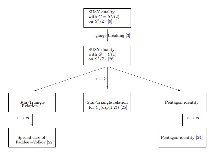
Figure 1: Structure of the paper.

The rest of this paper is organized as follows. In section 2, we briefly recollect some basic definitions. In section 3, we present the star-triangle relations and pentagon identities resulting from the supersymmetric duality. In section 4, we discuss how to relate our star-triangle relation to the one obtained in Hadasz:2013bwa . In section 5, we present our conclusions and discuss some open questions. We include three appendices for some technical details.

2 Lens partition function, 3d duality and gauge symmetry breaking

2.1 Supersymmetric partition function on $S^{3}_{b}/\mathbb{Z}_{r}$

We start by defining the general form of the three dimensional $\mathcal{N}=2$ partition function on the squashed lens space $S^{3}_{b}/\mathbb{Z}_{r}$. The lens partition function can be computed by a straightforward dimensional reduction of the four-dimensional lens superconformal index Benini:2011nc ; Yamazaki:2013fva ; Eren:2019ibl or via the supersymmetric localization technique Imamura:2012rq ; Imamura:2013qxa . Here we briefly outline some basic ingredients and refer the reader to Imamura:2012rq ; Imamura:2013qxa ; Nieri:2015yia ; Gahramanov:2016ilb for more details.

Recall that the lens space $S_{b}^{3}/\mathbb{Z}_{r}$ can be obtained from the squashed three sphere

$$S_{b}^{3}=\{(x,y)\in\mathbb{C}^{2},b^{2}|x|^{2}+b^{-2}|y|^{2}=1\}\>,$$ (3)

by making the identification $(x,y)\sim(e^{\frac{2\pi i}{r}}x,e^{\frac{2\pi i}{r}}y)$. The partition function on this manifold can be reduced to the following matrix model

$$Z=\sum_{y}\int\frac{1}{|W|}\prod_{j}^{rankG}\frac{dz_{j}}{2\pi ir}Z_{\text{classical}}[z,y]Z_{\text{one-loop}}[z,y]\;.$$ (4)

Here the sum is over the holonomies $y=\frac{r}{2\pi}\int_{C}A_{\mu}dx^{\mu}$, where $C$ is the non-trivial cycle on $S^{3}_{b}/\mathbb{Z}_{r}$ and $A_{\mu}$ is the gauge field. The integral is over the Cartan subalgebra of the gauge group and $z_{j}$ variables are corresponding to Weyl weights. The order of the group G is represented by the prefactor $|W|$ such that the gauge group is broken by the holonomy into a product of $r$ subgroups.

The one-loop contribution of chiral multiplets is given in terms of hyperbolic hypergeometric function,

$$Z_{\rm chiral}=\prod_{j}\prod_{\rho_{j}}\prod_{\phi_{j}}\hat{s}_{b,-\rho_{j}(y)-\phi_{j}(n)}\left(i\frac{Q}{2}(1-\Delta_{j})-\rho_{j}(z)-\phi_{j}(\Phi)\right)~{}.$$ (5)

Here $j$ labels chiral multiplets; $\rho_{j},\phi_{j}$, are the weights of the representation of the gauge and flavor groups, respectively and $\Delta_{j}$ is the Weyl weight of $j$’th chiral multiplet. We also define, $Q=b+\frac{1}{b}$ with the squashing parameter $b^{2}=\omega_{2}/\omega_{1}$. The function $\hat{s}_{b,y}(z)$ is a version of the improved double sine function Gahramanov:2016ilb , which can be written as a product of hyperbolic gamma functions

$$\hat{s}_{b,-y}(x)=\sigma_{h}(y)\gamma^{(2)}(iz+y\omega_{1}+\eta;\omega_{1}r,2\eta)\gamma^{(2)}(iz+\omega_{2}(r-y)+\eta;\omega_{2}r,2\eta)\;,$$ (6)

with $\sigma_{h}(y)=e^{\frac{i\pi}{2r}(y(r-y)-(r-1)y^{2})}$ and $\eta=(\omega_{1}+\omega_{2})/2$. For practical reasons, and in keeping with supersymmetric gauge theories notations, we will mainly use the hyperbolic gamma function $\gamma^{(2)}(z,\omega_{1},\omega_{2})$ instead of $\hat{s}_{b,y}(z)$. The one-loop contribution of the vector multiplet combined with the Vandermonde determinant can be written as

$$Z_{\rm vector}=\prod_{\alpha\in R_{+}}\frac{1}{\hat{s}_{b,\alpha(y)}\left(i\frac{Q}{2}+\alpha(z)\right)}\;,$$

where the product is over the positive roots $\alpha$ of the gauge group $G$. Once we know the group-theoretical data of three-dimensional supersymmetric theory on $S_{b}^{3}/\mathbb{Z}_{r}$, we can write down the partition function in terms of hyperbolic hypergeometric integral. Note that in our examples the classical term $Z_{\text{classical}}$ which includes the contributions coming from classical action of the Chern-Simons term and Fayet-Iliopoulos term will be absent. We should mention that the expressions for multiplets are the same as the one used in Gahramanov:2016ilb ; Eren:2019ibl and differs by some factor (the partition function is the same) from that in Imamura:2012rq and Nieri:2015yia . The relation between two expressions can be found in Gahramanov:2016ilb and in Appendix A.

2.2 Three-dimensional $\mathcal{N}=2$ IR duality

We will perform the gauge symmetry breaking of the following three-dimensional $\mathcal{N}=2$ supersymmetric dual theories:

• Theory A, has gauge group $SU(2)$ and flavor group $SU(6)$. The chiral multiplets transform under the fundamental representation of the gauge group and the flavor group; the vector multiplet transforms under the adjoint representation of the gauge group.

• Theory B, is the dual to the theory A without gauge symmetry. There are fifteen chiral multiplets in the totally antisymmetric tensor representation of the flavor group. In our case, Theory B is the low energy description of Theory A which can be characterized purely by composite gauge singlets.

Because of the supersymmetric duality one obtains the following equality of the partition functions Gahramanov:2016ilb

$$\frac{1}{2r\sqrt{-\omega_{1}\omega_{2}}}\sum_{y=0}^{[r/2]}\epsilon(y)\int_{-\infty}^{\infty}dz \frac{\prod_{i=1}^{6}\gamma^{(2)}(-i(a_{i}\pm z)-i\omega_{1}(u_{i}\pm y);-i\omega_{1}r,-i\omega_{1}-i\omega_{2})}{\gamma^{(2)}(\mp 2iz\mp 2i\omega_{1}y;-i\omega_{1}r,-i\omega_{1}-i\omega_{2})}$$

$$\times \frac{\gamma^{(2)}(-i(a_{i}\pm z)-i\omega_{2}(r-(u_{i}\pm y));-i\omega_{2}r,-i\omega_{1}-i\omega_{2})}{\gamma^{(2)}(\mp 2iz-i\omega_{2}(r\mp 2y);-i\omega_{2}r,-i\omega_{1}-i\omega_{2})}$$

$$=\prod_{1\leq i<j\leq 6} \gamma^{(2)}(-i(a_{i}+a_{j})-i\omega_{1}(u_{i}+u_{j});-i\omega_{1}r,-i\omega_{1}-i\omega_{2})$$

$$\gamma^{(2)}(-i(a_{i}+a_{j})-i\omega_{2}(r-(u_{i}+u_{j}));-i\omega_{2}r,-i\omega_{1}-i\omega_{2})\;,$$ (7)

with the balancing conditions $\sum^{6}_{i=1}a_{i}=\omega_{1}+\omega_{2}$ and $\sum_{i=1}^{6}u_{i}=0$. We should mention that there is a contribution of the $R$-symmetry appearing in the partition function but we absorbed it in the flavor fugacity. Since all physical degrees of freedom of Theory B are gauge invariant there is no summation and integration on the right hand side of the identity. The case $r=1$ of the integral identity (2.2) is a very well-known integral identity, see, e.g. van2007hyperbolic , in this case it corresponds to the equality of the squashed three-sphere partition functions Hama:2011ea .

The hyperbolic hypergeometric beta sum-integral (2.2) is an important identity in the theory of hyperbolic hypergeometric functions. Its role in integrable models of statistical mechanics was discovered in Gahramanov:2016ilb .

2.3 Gauge Symmetry Breaking

Now we are in a position to obtain new dual theories by breaking the gauge symmetry. The idea is to break the gauge symmetry from $SU(2)$ to $U(1)$ in dual theories presented above. We give a VEV to two flavor quarks, breaking the gauge group to $U(1)$ and reducing the flavor group to $SU(3)\times SU(3)$. As a result we obtain the following dual theories:

• Theory A: $3d$ $\mathcal{N}=2$ theory with $U(1)$ gauge symmetry and $SU(3)_{L}\times SU(3)_{R}$ flavor group, chiral multiplets are belonging to the $SU(3)_{L}$ transforming in the fundamental representation of the gauge group and chiral multiplets are belonging to the $SU(3)_{R}$, transforming in the anti-fundamental representation.

• Theory B: The dual theory has the same global symmetries without gauge degrees of freedom, nine “mesons”, transforming in the fundamental representation of the flavor group $SU(3)_{L}\times SU(3)_{R}$.

We make the breaking of gauge symmetry on the level of partition functions. Following the work Spiridonov:2010em (see also Sarkissian:2018ppc ) let us replace the flavor fugacities $a_{i}$ to $a_{i}+\mu$ for $i=\{1,2,3\}$ and $a_{i}-\mu$ for $i=\{4,5,6\}$. We use the fact that the identity (2.2) is symmetric with respect to $z\rightarrow-z$ transformation. By changing the variable $z$ to $z+\mu$ we get the following expression

$$\frac{1}{r\sqrt{-\omega_{1}\omega_{2}}}\sum_{y=0}^{[r/2]}\epsilon(y)\int_{-\mu}^{\infty}dz \frac{\prod_{i=1}^{3}\gamma^{(2)}(-i(a_{i}+\mu\pm(z+\mu))-i\omega_{1}(u_{i}\pm y);-i\omega_{1}r,-i\omega_{1}-i\omega_{2})}{\gamma^{(2)}(\mp 2i(z+\mu)\mp 2i\omega_{1}y;-i\omega_{1}r,-i\omega_{1}-i\omega_{2})}$$

$$\times \frac{\gamma^{(2)}(-i(a_{i}+\mu\pm(z+\mu))-i\omega_{2}(r-(u_{i}\pm y));-i\omega_{2}r,-i\omega_{1}-i\omega_{2})}{\gamma^{(2)}(\mp 2i(z+\mu)-i\omega_{2}(r\mp 2y);-i\omega_{2}r,-i\omega_{1}-i\omega_{2})}$$

$$\prod_{i=4}^{6} \gamma^{(2)}(-i(a_{i}-\mu\pm(z+\mu))-i\omega_{1}(u_{i}\pm y);-i\omega_{1}r,-i\omega_{1}-i\omega_{2})$$

$$\times \gamma^{(2)}(-i(a_{i}-\mu\pm(z+\mu))-i\omega_{2}(r-(u_{i}\pm y));-i\omega_{2}r,-i\omega_{1}-i\omega_{2})$$

$$=\prod_{i=1}^{3}\prod_{j=4}^{6} \gamma^{(2)}(-i(a_{i}+a_{j})-i\omega_{1}(u_{i}+u_{j});-i\omega_{1}r,-i\omega_{1}-i\omega_{2})$$

$$\times \gamma^{(2)}(-i(a_{i}+a_{j})-i\omega_{2}(r-(u_{i}+u_{j}));-i\omega_{2}r,-i\omega_{1}+\omega_{2})$$

$$\prod_{1\leq i<j\leq 3} \gamma^{(2)}(-i(a_{i+3}+a_{j+3}-2\mu)-i\omega_{2}(r-(u_{i+3}+u_{j+3}));-i\omega_{2}r,-i\omega_{1}-i\omega_{2})$$

$$\times \gamma^{(2)}(-i(a_{i}+a_{j}+2\mu)-i\omega_{2}(r-(u_{i}+u_{j}));-i\omega_{2}r,-i\omega_{1}-i\omega_{2})$$

$$\times \gamma^{(2)}(-i(a_{i+3}+a_{j+3}-2\mu)-i\omega_{1}(u_{i+3}+u_{j+3});-i\omega_{1}r,-i\omega_{1}-i\omega_{2})$$

$$\times \gamma^{(2)}(-i(a_{i}+a_{j}+2\mu)-i\omega_{1}(u_{i}+u_{j});-i\omega_{1}r,-i\omega_{1}-i\omega_{2})\>.$$ (8)

After taking the limit $\mu\to\infty$ and renaming the flavor group coefficients as $a_{i}=b_{i}$ and $u_{i}=v_{i}$ for only $i\in\{4,5,6\}$, the reduced form of the hyperbolic hypergeometric integral identity turns out to be

$$\frac{1}{r\sqrt{-\omega_{1}\omega_{2}}}\sum_{y=0}^{[r/2]}\epsilon(y)e^{\frac{\pi iC}{2}}\int_{-\infty}^{\infty}dz\prod_{i=1}^{3} \gamma^{(2)}(-i(a_{i}-z)-i\omega_{1}(u_{i}-y);-i\omega_{1}r,-i\omega_{1}-i\omega_{2})$$

$$\times \gamma^{(2)}(-i(a_{i}-z)-i\omega_{2}(r-(u_{i}-y));-i\omega_{2}r,-i\omega_{1}-i\omega_{2})$$

$$\times \gamma^{(2)}(-i(b_{i}+z)-i\omega_{1}(v_{i}+y);-i\omega_{1}r,-i\omega_{1}-i\omega_{2})$$

$$\times \gamma^{(2)}(-i(b_{i}+z)-i\omega_{2}(r-(v_{i}+y));-i\omega_{2}r,-i\omega_{1}-i\omega_{2})$$

$$=\prod_{i,j=1}^{3} \gamma^{(2)}(-i(a_{i}+b_{j})-i\omega_{1}(u_{i}+v_{j});-i\omega_{1}r,-i\omega_{1}-i\omega_{2})$$

$$\times \gamma^{(2)}(-i(a_{i}+b_{j})-i\omega_{2}(r-(u_{i}+v_{j}));-i\omega_{2}r,-i\omega_{1}-i\omega_{2}))\;,$$ (9)

with the balancing conditions $\sum_{i=1}^{3}a_{i}+b_{i}=\omega_{1}+\omega_{2}$ and $\sum_{i=1}^{3}u_{i}+v_{i}=0$. Here $C=-2y+(u_{1}+u_{2}+u_{3}-v_{1}-v_{2}-v_{3})$. On the left hand-side of the integral identity, we see the partition function of the Theory A and on the right hand-side, the Theory B. A similar identity was discussed for the $S_{b}^{3}$ sphere partition functions in Spiridonov:2010em ; Kashaev:2012cz and for the superconformal indices in Gahramanov:2013rda ; Gahramanov:2014ona ; Gahramanov:2016wxi . The integral identity (9) is essentially the same integral identity as the one obtained in Sarkissian:2018ppc with a slightly different sign coefficient.

3 Star-triangle relation and pentagon identity

In this section we investigate the relation between supersymmetric dualities, integrability and triangulated 3-manifolds. We will show that the integral identity (9) can be written as the star-triangle relation and as the integral pentagon identity.

3.1 Pentagon Identity

The integral identity (9) can be written as a pentagon relation. The pentagon identity usually represents the basic 2-3 Pachner move pachner1991pl for a certain triangulated 3-manifold. There are several examples of integral pentagon relations computed via three-dimensional supersymmetric dualities, see, e.g. Dimofte:2011ju ; Kashaev:2012cz ; Gahramanov:2013rda ; Gahramanov:2014ona ; Gahramanov:2016wxi ; Benvenuti:2016wet ; Bozkurt:2018xno ; Jafarzade:2018yei . Here we present a new pentagon identity in terms of hyperbolic gamma functions.

It is convenient to define the following function

$$\mathcal{B}(z_{1},u_{1};z_{2},u_{2})=\frac{\gamma^{(2)}(-iz_{1}-i\omega_{1}u_{1};-i\omega_{1}r,-i\omega_{1}-i\omega_{2})\gamma^{(2)}(-iz_{1}-i\omega_{2}(r-u_{1});-i\omega_{2}r,-i\omega_{1}-i\omega_{2})}{\gamma^{(2)}(-i(z_{1}+z_{2})-i\omega_{1}(u_{1}+u_{2});-i\omega_{1}r,-i\omega_{1}-i\omega_{2})}$$

$$\frac{\gamma^{(2)}(-iz_{2}-i\omega_{1}u_{2};-i\omega_{1}r,-i\omega_{1}-i\omega_{2})\gamma^{(2)}(-iz_{2}-i\omega_{2}(r-u_{2});-i\omega_{2}r,-i\omega_{1}-i\omega_{2})}{\gamma^{(2)}(-i(z_{1}+z_{2})-i\omega_{2}(r-u_{1}-u_{2});-i\omega_{2}r,-i\omega_{1}-i\omega_{2})}\;,$$ (10)

which solves the following integral pentagon identity,

$$\frac{1}{r\sqrt{-\omega_{1}\omega_{2}}}\sum_{y=-\lfloor r/2\rfloor}^{\lfloor r/2\rfloor}e^{\frac{\pi iC}{2}}\int_{-\infty}^{\infty}dz\prod_{i=1}^{3}\mathcal{B}(a_{i}-z,u_{i}-y;b_{i}+z,v_{i}+y)$$

$$=\mathcal{B}(a_{1}+b_{2},u_{1}+v_{2};a_{2}+b_{3},u_{2}+v_{3})\mathcal{B}(a_{1}+b_{3},u_{1}+v_{3};a_{2}+b_{1},u_{2}+v_{1})$$ (11)

with the same balancing conditions given in (9).

3.2 Limit of the Pentagon Identity

There are several pentagon identities in terms of Euler’s gamma function Kashaev:2012cz ; kashaev2014euler ; Jafarzade:2018yei . Here we present the pentagon relation found in Jafarzade:2018yei in terms of gamma function which we obtain in a different manner.

In order to explore the limit of the pentagon identity we use the following asymptotic relation

$$\lim_{\omega_{2}\to\infty}\Big{(}\frac{\omega_{2}}{2\pi\omega_{1}}\Big{)}^{\frac{z}{\omega_{2}}-\frac{1}{2}}\gamma^{(2)}(z;\omega_{1},\omega_{2})=\frac{\Gamma(z/\omega_{1})}{\sqrt{2\pi}}\;.$$ (12)

We identify $\omega_{1}$ with $\omega_{2}$ and redefine all coefficients dividing by $\frac{\omega_{1}+\omega_{2}}{\omega_{1}}$, then by altering $\frac{a_{i}-z}{\omega_{1}}$ to $a_{i}-z$, we obtain the limit of the pentagon identity as follows

$$\sum_{y=-\infty}^{\infty}\int_{-\infty}^{\infty}\frac{dz}{4\pi i}\prod_{i=1}^{3}\frac{\Gamma\left(a_{i}-z+\frac{u_{i}-y}{2}\right)\Gamma\left(b_{i}+z+\frac{v_{i}+y}{2}\right)\Gamma\left(1-a_{i}-b_{i}+\frac{u_{i}+v_{i}}{2}\right)}{\Gamma\left(1-b_{i}-z+\frac{v_{i}+y}{2}\right)\Gamma\left(1-a_{i}+z+\frac{u_{i}-y}{2}\right)\Gamma\left(a_{i}+b_{i}+\frac{u_{i}+v_{i}}{2}\right)}$$

$$=\prod_{i,j=1;i\neq j}^{3}\frac{\Gamma\left(a_{i}+b_{j}+\frac{u_{i}+v_{j}}{2}\right)}{\Gamma\left(1-a_{i}-b_{j}+\frac{u_{i}+v_{j}}{2}\right)}\;.$$ (13)

If we introduce the following function

$$\mathcal{B}(z_{1},u_{1};z_{2},u_{2})=\frac{\Gamma\left(z_{1}+\frac{u_{1}}{2}\right)\Gamma\left(z_{2}+\frac{u_{2}}{2}\right)\Gamma\left(1-z_{1}-z_{2}-\frac{u_{1}+u_{2}}{2}\right)}{\Gamma\left(z_{1}+z_{2}+\frac{u_{1}+u_{2}}{2}\right)\Gamma\left(1-z_{1}-\frac{u_{1}}{2}\right)\Gamma\left(1-z_{2}-\frac{u_{2}}{2}\right)}\;,$$ (14)

one obtains the integral pentagon identity

$$\sum^{\infty}_{y=-\infty}\int_{-\infty}^{\infty}\frac{dz}{4\pi i}\prod_{i=1}^{3} \mathcal{B}(a_{i}-z,u_{i}-y;b_{i}+z,v_{i}+y)$$

$$= \mathcal{B}(a_{1}+b_{3},u_{1}+v_{3};a_{2}+b_{1},u_{2}+v_{1})\mathcal{B}(a_{1}+b_{2},u_{1}+v_{2};a_{2}+b_{3},u_{1}+v_{3})\;.$$ (15)

This is exactly the result obtained in Jafarzade:2018yei via dimensional reduction of the three-dimensional $\mathcal{N}=2$ supersymmetric dual theories on $S^{2}\times S^{1}$.

3.3 Star-triangle relation

The star-triangle relation is a crucial equation in the study of two-dimensional integrable lattice spin models. Here we obtain solution to the star-triangle relation mentioned in Sarkissian:2018ppc . We fix the parameters as

$$a_{i} =-\alpha_{i}+x_{i}\;,~{}~{}~{}~{}~{}~{}~{}~{}~{}~{}~{}~{}~{}\;b_{i}=-\alpha_{i}-x_{i}\;,$$ (16)

and we insert the condition $u_{i}=-v_{i}$. By defining the Boltzmann weight as

$$W_{\alpha}(x_{i},x_{j},u_{i},u_{j})= e^{-\pi i(u_{i}+u_{j})}\gamma^{(2)}(-i(-\alpha+x_{i}-x_{j})-i\omega_{1}(u_{i}-u_{j});-i\omega_{1}r,-i\omega_{1}-i\omega_{2})$$

$$\gamma^{(2)}(-i(-\alpha+x_{i}-x_{j})-i\omega_{2}(r-(u_{i}-u_{j}));-i\omega_{2}r,-i\omega_{1}-i\omega_{2})$$

$$\gamma^{(2)}(-i(-\alpha-x_{i}+x_{j})-i\omega_{1}(u_{j}-u_{i});-i\omega_{1}r,-i\omega_{1}-i\omega_{2})$$

$$\gamma^{(2)}(-i(-\alpha-x_{i}+x_{j})-i\omega_{2}(r-(u_{j}-u_{i}));-i\omega_{2}r,-i\omega_{1}-i\omega_{2})\;$$ (17)

and the spin-independent weight as

$$R(\alpha_{1},\alpha_{2},\alpha_{3})=\prod_{j=1}^{3}\gamma^{(2)}(2i\alpha_{j};-i\omega_{1}r,-i(\omega_{1}+\omega_{2}))\gamma^{(2)}(2i\alpha_{j};-i\omega_{2}r,-i(\omega_{1}+\omega_{2}))\;,$$ (18)

one can rewrite the integral identity (9) as the following star-triangle relation

$$\frac{1}{r\sqrt{-\omega_{1}\omega_{2}}}\sum_{y=-\lfloor r/2\rfloor}^{\lfloor r/2\rfloor}e^{-2\pi iy}\int_{-\infty}^{\infty}dzW_{\alpha_{1}}(x_{1},z,u_{1},y)W_{\alpha_{2}}(x_{2},z,u_{2},y)W_{\alpha_{3}}(x_{3},z,u_{3},y)$$

$$=R(\alpha_{1},\alpha_{2},\alpha_{3})W_{\alpha_{1}+\alpha_{2}}(x_{1},x_{2},u_{1},u_{2})W_{\alpha_{1}+\alpha_{3}}(x_{1},x_{3},u_{1},u_{3})W_{\alpha_{2}+\alpha_{3}}(x_{2},x_{3},u_{2},u_{3})\;.$$ (19)

Our model is an Ising type model where sites of the lattice are assigned to discrete $y$ and continuous spin $z$ variables.

3.4 Limit of the Star-Triangle Relation

There are several solutions to the star-triangle relation in terms of Euler’s gamma function. In our case such a solution can be achieved by taking the limit (12). After taking the limit, we obtain the following Boltzmann weight

$$W_{\theta}(x,z,u,y)=\frac{\Gamma(\frac{1-\frac{\theta}{\pi}+ix-iz+u-y}{2})\Gamma(\frac{1-\frac{\theta}{\pi}-ix+iz+v+y}{2})}{\Gamma(\frac{1+\frac{\theta}{\pi}+ix-iz-u+y}{2})\Gamma(\frac{1+\frac{\theta}{\pi}-ix+iz-u+y}{2})}\;,$$ (20)

and spin independent weight

$$R(\theta_{1},\theta_{2},\theta_{3})=\prod_{i=1}^{3}\frac{\Gamma(1-\frac{\theta_{i}}{\pi})}{\Gamma(\frac{\theta_{i}}{\pi})}\;.$$ (21)

The star-triangle relation can be written as

$$\sum_{y=-\infty}^{\infty}\int_{-\infty}^{\infty}\frac{dz}{8\pi}W_{\theta_{1}}(x_{1},z,u_{1},y)W_{\theta_{2}}(x_{2},z,u_{2},y)W_{\theta_{3}}(x_{3},z,u_{3},y)$$

$$=R(\theta_{1},\theta_{2},\theta_{3})W_{\pi-\theta_{1}}(x_{2},x_{3},u_{2},u_{3})W_{\pi-\theta_{2}}(x_{1},x_{3},u_{1},u_{3})W_{\pi-\theta_{3}}(x_{1},x_{2},u_{1},u_{2})\;,$$ (22)

where $\theta_{1}+\theta_{2}+\theta_{3}=2\pi$. It can be easily checked that this solution is exactly the one obtained in Bazhanov:2007vg from the Faddeev-Volkov model. In Bazhanov:2007vg authors normalized the Boltmann weights (20) in such a way that the spin-independent function $R(\theta_{1},\theta_{2},\theta_{3})$ is equal to one. Note that the solution (20) is related to the special case of the Zamolodchikov’s “fishnet” model Zamolodchikov:1980mb ; Bazhanov:2007vg ; Bazhanov:2016ajm .

4 Relation to the $U_{q}(\text{osp}(1|2))$

It is well known that the unitary representations of the modular double of $U_{q}(sl(2,R))$ is equivalent to the representations of the Liouville theory. For instance, $3j$-symbols for the tensor product of modular double representations of $U_{q}(sl(2,R))$ appear in the fusion product for the Liouville vertex operators. The modular double representation for the $U_{q}(osp(1|2))$ plays the same role in the $\mathcal{N}=1$ supersymmetric Liouville theory.

Here we show how one can obtain the star-triangle relation for the $U_{q}(osp(1|2))$ Pawelkiewicz:2013wga ; Hadasz:2013bwa (see also Poghosyan:2016kvd ) from the integral identity (9). The computations presented here and in Appendix C overlap with the computations of Sarkissian:2018ppc . We use different notations and present all calculations in detail, see Appendix C. From the supersymmetric gauge theory point of view, the star-triangle relation represents the equality of partition functions of dual three-dimensional $\mathcal{N}=2$ gauge theories on $S_{b}^{3}/Z_{2}$ (it is topologically $\mathbb{RP}^{3}$). Similar computations for the Liouville field theory and the supersymmetric gauge theories on squashed three-sphere $S_{b}^{3}$ was performed in Teschner:2012em .

A special case of the expression (9) when r = 2, gives the star-triangle relation discussed in Hadasz:2013bwa which can be used for proving orthogonality and completeness relation of the Clebsch-Gordan coefficients for the self-dual continuous series of $U_{q}(osp(1|2))$ and the $\mathcal{N}=1$ supersymmetric Liouville theory. For the special case $r=2$ we obtain the following expression

$$\sum_{\nu=0,1}(-1)^{\frac{2\nu-3-\sum_{i}(\mu_{i}-\nu_{i})}{2}}\int\frac{dx}{i}\prod_{i=1}^{3}S_{\nu+\nu_{i}}(x+a_{i})S_{1+\nu+\mu_{i}}(b_{i}-x)=2\prod_{i,j=1}^{3}S_{1+\nu_{i}+\mu_{j}}(a_{i}+b_{j})\;,$$ (23)

where we introduced the notations of the work Hadasz:2013bwa

$$S_{\nu}(x)=\gamma^{(2)}(\frac{x+(1-\nu)b}{2},b,\frac{1}{b})\gamma^{(2)}(\frac{x+1/b+\nu b}{2},b,\frac{1}{b})\;.$$ (24)

Note that we have a different sign coefficient in (23) than in Hadasz:2013bwa ; Sarkissian:2018ppc . It seems that one can obtain the integral identity (5.14) from the work Hadasz:2007wi by tending one of the flavor fugacities to $b+\frac{1}{b}$.

5 Conclusion

We obtain the pentagon identity (11) (related to the Heisenberg double) and the star-triangle relation (19) (related to the quantum algebra) from the same integral identity. Note that it is possible to construct the Boltzmann weight $W$ (17) from the $B$-function (10), see e.g. kashaev1997heisenberg ; Faddeev:1999fe ; hikami2001hyperbolic .

There are several directions that we wish to pursue in the future. We showed that, by performing a suitable identification, our star-triangle relation gives the same identity obtained in Hadasz:2013bwa . This result is interesting not only because it builds a relation between two different subjects, but also it can be applied to arbitrary $r$. The problem we leave to the future is the construction of the corresponding quantum algebra for the integral identity (22) with the general $r$.

In this work we presented rational and trigonometric solutions to the Yang–Baxter equation in the form called star-triangle relation. It would be interesting to construct the operator form of the Yang-Baxter equation and the Hamiltonian of the one-dimensional chain corresponding to this solution.

The pentagon identity and the star-triangle relation are a consequence of the Heisenberg double and the quantum algebra, respectively. We should mention that the appearance of the pentagon relation refers to the Pachner’s move for triangulated 3-manifolds, though, we do not know how to construct this relation formally.

Appendix A Properties of special functions

Here we present several definitions and notations of special functions needed in this work.

We briefly summarize the basic properties of hyperbolic gamma function and its different notations van2007hyperbolic ; Andersen:2014aoa . This function appears in several areas of mathematical and theoretical physics, here is an incomplete list of these topics.

• knot theory hikami2001hyperbolic ; Hikami_2007 ; hikami2014braiding ; Chan:2017qnw

• supersymmetric gauge theory Teschner:2012em

• integrable models of statistical mechanics Bazhanov:2007mh ; Bazhanov:2007vg

• special functions van2007hyperbolic

With parameters $\tilde{q}=e^{2\pi i\omega_{1}/\omega_{2}}$ and $q=e^{-2\pi i\omega_{2}/\omega_{1}}$, the infinite product representation is

$$\gamma^{(2)}(z;\omega_{1},\omega_{2})=e^{\frac{\pi i}{2}B_{2,2}(z;\omega_{1},\omega_{2})}\frac{(e^{-2\pi i\frac{z}{\omega_{2}}}\tilde{q};\tilde{q})}{(e^{-2\pi i\frac{z}{\omega_{1}}};q)}\;,$$ (25)

where we have one of the Bernoulli polynomials,

$$B_{2,2}(z;\omega_{1},\omega_{2})=\frac{z^{2}-z(\omega_{1}+\omega_{2})}{\omega_{1}\omega_{2}}+\frac{\omega_{1}^{2}+3\omega_{1}\omega_{2}+\omega_{2}^{2}}{6\omega_{1}\omega_{2}}.$$ (26)

Here, we realise that $B_{2,2}(z;\omega_{1},\omega_{2})$ is crucial for the asymptotic behavior of the hyperbolic gamma function. The hyperbolic gamma function has an integral representation

$$\gamma^{(2)}(z;\omega_{1},\omega_{2})=\exp{\left(-\int_{0}^{\infty}\frac{dx}{x}\left[\frac{\sinh{x(2z-\omega_{1}-\omega_{2})}}{2\sinh{(x\omega_{1})}\sinh{(x\omega_{2})}}-\frac{2z-\omega_{1}-\omega_{2}}{2x\omega_{1}\omega_{2}}\right]\right)}\;,$$ (27)

where $Re(\omega_{1}),Re(\omega_{2})>0$ and $Re(\omega_{1}+\omega_{2})>Re(z)>0$.
We list here some properties of this function.

Symmetry: $$\gamma^{(2)}(z;\omega_{1},\omega_{2})=\gamma^{(2)}(z;\omega_{2},\omega_{1})$$ (28)

Reflection: $$\gamma^{(2)}(z;\omega_{1},\omega_{2})\gamma^{(2)}(\omega_{1}+\omega_{2}-z;\omega_{1},\omega_{2})=1$$ (29)

Scaling: $$\gamma^{(2)}(z;\omega_{1},\omega_{2})=\gamma^{(2)}(uz;u\omega_{1},u\omega_{2})$$ (30)

Conjugation: $$\gamma^{(2)}(z;\omega_{1},\omega_{2})^{*}=\gamma^{(2)}(z^{*};\omega_{2}^{*},\omega_{1}^{*})$$ (31)

Another very important property of the hyperbolic gamma function is the following difference equation

$$\gamma^{(2)}(z+\omega_{1};\omega_{1},\omega_{2})=e^{-\frac{\pi i}{2}\left(B_{2,2}(z+\omega_{1};\omega)-B_{2,2}(z;\omega)\right)}(1-e^{2\pi i\frac{z}{\omega_{2}}})\gamma^{(2)}(z;\omega_{1},\omega_{2})\;,$$ (32)

after simplifying, the difference equation takes the form,

$$\gamma^{(2)}(z+\omega_{1};\omega_{1},\omega_{2})=2\sin\left(\frac{\pi z}{\omega_{2}}\right)\gamma^{(2)}(z;\omega_{1},\omega_{2})\;.$$ (33)

Now we introduce the asymptotic behaviour of the function

$$\lim_{z\to\infty}e^{\frac{\pi i}{2}B_{2,2}(z;\omega_{1},\omega_{2})}\gamma^{(2)}(z;\omega_{1},\omega_{2})=1\>\>\text{for}\>\>\arg{\omega_{2}+\pi}>\arg{z}>\arg{\omega_{1}}$$ (34)

$$\lim_{z\to\infty}e^{-\frac{\pi i}{2}B_{2,2}(z;\omega_{1},\omega_{2})}\gamma^{(2)}(z;\omega_{1},\omega_{2})=1\>\>\text{for}\>\>\arg{\omega_{2}}>\arg{z}>\arg{\omega_{1}-\pi}\;,$$ (35)

where $\text{Im}(\frac{\omega_{1}}{\omega_{2}})>0$. We use these formulas for the breaking of gauge symmetry given in Appendix B.

There is a generalization of the hyperbolic gamma function $\Gamma_{h}(z,y;\omega_{1},\omega_{2})$ which was introduced in Gahramanov:2016ilb . This function can be defined in terms of $\gamma^{(2)}(z;\omega_{1},\omega_{2})$ as follows

$$\Gamma_{h}(z,y;\omega_{1},\omega_{2})=e^{\phi(y)}\gamma^{(2)}(-iz-i\omega_{1}y;-i\omega_{1}r,-i(\omega_{1}+\omega_{2}))\gamma^{(2)}(-iz-i\omega_{2}(r-y);-i\omega_{2}r,-i(\omega_{1}+\omega_{2}))\;,$$ (36)

where $\phi(y)=-\frac{\pi i}{6r}(2y^{3}-3y^{2}r+yr^{2})$. It has the following properties.

Symmetry and Reflection: $$\Gamma_{h}(z,y;\omega_{1},\omega_{2})\Gamma_{h}(\omega_{1}+\omega_{2}-z,y;\omega_{2},\omega_{1})=e^{2\phi(y)}$$ (37)

Scaling: $$\frac{\Gamma_{h}(uz,uy;u\omega_{1},u\omega_{2})}{\Gamma_{h}(z,y;\omega_{2},\omega_{1})}=e^{\phi(uy)-\phi(y)}$$ (38)

Conjugation: $$\Gamma_{h}(z,y;\omega_{1},\omega_{2})^{*}=\Gamma_{h}(z^{*},y^{*};\omega_{2}^{*},\omega_{1}^{*})$$ (39)

Appendix B Gauge Symmetry Breaking

We start by reparemetrizing the integral identity coming from the duality argument, given in (9)

$$\frac{1}{2r\sqrt{-\omega_{1}\omega_{2}}}\sum_{y=0}^{[r/2]}\epsilon(y)\int_{-\infty}^{\infty}dz\frac{\prod_{i=1}^{6}\gamma^{(2)}(-i(a_{i}\pm z)-i\omega_{1}(u_{i}\pm y);-i\omega_{1}r,-i(\omega_{1}+\omega_{2}))}{\gamma^{(2)}(\mp 2iz\mp i\omega_{1}(2y);-i\omega_{1}r,-i(\omega_{1}+\omega_{2}))}$$

$$\times\frac{\gamma^{(2)}(-i(a_{i}\pm z)-i\omega_{2}(r-(u_{i}\pm y));-i\omega_{2}r,-i(\omega_{1}+\omega_{2}))}{\gamma^{(2)}(\mp 2iz-i\omega_{2}(r\mp(2y));-i\omega_{2}r,-i(\omega_{1}+\omega_{2}))}$$

$$=\prod_{1\leq i<j\leq 6}\gamma^{(2)}(-i(a_{i}+a_{j})-i\omega_{1}(u_{i}+u_{j});-i\omega_{1}r,-i(\omega_{1}+\omega_{2}))$$

$$\gamma^{(2)}(-i(a_{i}+a_{j})-i\omega_{2}(r-(u_{i}+u_{j}));-i\omega_{2}r,-i(\omega_{1}+\omega_{2}))\;,$$ (40)

with the balancing condition $\sum^{6}_{i=1}a_{i}=\omega_{1}+\omega_{2}$ and $\sum_{i=1}^{6}u_{i}=0$.

As we add $\mu$ to first three coefficients and z variable, coming from the fundamental representation of the flavor group and gauge group; subtract $\mu$ from the last three coefficients, the left hand side of the equation turns out to be

$$\frac{1}{r\sqrt{-\omega_{1}\omega_{2}}}\sum_{y=0}^{[r/2]}\epsilon(y)\int_{-\mu}^{\infty}dz\prod_{i=1}^{3}\gamma^{(2)}(-i(a_{i}-z)-i\omega_{1}(u_{i}-y);-i\omega_{1}r,-i(\omega_{1}+\omega_{2}))$$

$$\times\gamma^{(2)}(-i(a_{i}-z))-i\omega_{2}(r-(u_{i}-y));-i\omega_{2}r,-i(\omega_{1}+\omega_{2}))$$

$$\times\prod_{i=4}^{6}\gamma^{(2)}(-i(a_{i}+z)-i\omega_{1}(u_{i}+y);-i\omega_{1}r,-i(\omega_{1}+\omega_{2}))$$

$$\times\gamma^{(2)}(-i(a_{i}+z)-i\omega_{2}(r-(u_{i}+y));-i\omega_{2}r,-i(\omega_{1}+\omega_{2}))$$

$$\Bigg{[}\frac{\prod_{i=1}^{3}\gamma^{(2)}(-i(a_{i}+z+2\mu)-i\omega_{1}(u_{i}+y);-i\omega_{1}r,-i(\omega_{1}+\omega_{2}))}{\gamma^{(2)}(\mp 2i(z+\mu)\mp i\omega_{1}(2y);-i\omega_{1}r,-i(\omega_{1}+\omega_{2}))}$$

$$\times\frac{\gamma^{(2)}(-i(a_{i}+z+2\mu)-i\omega_{2}(r-(u_{i}+y));-i\omega_{2}r,-i(\omega_{1}+\omega_{2}))}{\gamma^{(2)}(\mp 2i(z+\mu)-i\omega_{2}(r\mp(2y));-i\omega_{2}r,-i(\omega_{1}+\omega_{2}))}$$

$$\prod_{i=4}^{6}\gamma^{(2)}(-i(a_{i}-z-2\mu)-i\omega_{1}(u_{i}-y);-i\omega_{1}r,-i(\omega_{1}+\omega_{2}))$$

$$\times\gamma^{(2)}(-i(a_{i}-z-2\mu)-i\omega_{2}(r-(u_{i}-y));-i\omega_{2}r,-i(\omega_{1}+\omega_{2}))\Bigg{]}\;.$$

Main idea is to transform the gauge group from $SU(2)$ to $U(1)$. In order to achieve this goal we will use the asymptotic relations of the special function $\gamma^{(2)}(z;\omega_{1},\omega_{2})$. Furthermore, as an outcome we will observe that there is a transformation in flavor group as well. After the process we also have the following right hand side

$$=\prod_{i=1}^{3}\prod_{j=4}^{6}\gamma^{(2)}(-i(a_{i}+a_{j})-i\omega_{1}(u_{i}+u_{j});-i\omega_{1}r,-i(\omega_{1}+\omega_{2}))$$

$$\gamma^{(2)}(-i(a_{i}+a_{j})-i\omega_{2}(r-(u_{i}+u_{j}));-i\omega_{2}r,-i(\omega_{1}+\omega_{2}))$$

$$\Big{[}\prod_{1\leq i<j\leq 3}\gamma^{(2)}(-i(a_{i}+a_{j}+2\mu)-i\omega_{1}(u_{i}+u_{j});-i\omega_{1}r,-i(\omega_{1}+\omega_{2}))$$

$$\gamma^{(2)}(-i(a_{i}+a_{j}+2\mu)-i\omega_{2}(r-(u_{i}+u_{j}));-i\omega_{2}r,-i(\omega_{1}+\omega_{2}))$$

$$\gamma^{(2)}(-i(a_{i+3}+a_{j+3}-2\mu)-i\omega_{1}(u_{i+3}+u_{j+3});-i\omega_{1}r,-i(\omega_{1}+\omega_{2}))$$

$$\gamma^{(2)}(-i(a_{i+3}+a_{j+3}-2\mu)-i\omega_{2}(r-(u_{i+3}+u_{j+3}));-i\omega_{2}r,-i(\omega_{1}+\omega_{2}))\Big{]}\;.$$ (41)

Here, from the asymptotic relations which hyperbolic gamma function satisfy, each term in the brackets behaves in a particular way,

$$e^{(\frac{2i\pi}{r}(\mu+z)(\omega_{1}^{-1}+\omega_{2}^{-1})+2i\pi y)}\gamma^{(2)}(\mp 2i(z+\mu)\mp i\omega_{1}(2y);-i\omega_{1}r,-i(\omega_{1}+\omega_{2}))^{-1}$$

$$\gamma^{(2)}(\mp 2i(z+\mu)\mp i\omega_{2}(r-2y);-i\omega_{2}r,-i(\omega_{1}+\omega_{2}))^{-1}\xrightarrow{\mu\to\infty}1\;,$$ (42)

and

$$\prod_{i=1}^{3}~{} \gamma^{(2)}(-i(a_{i}+z+2\mu)-i\omega_{1}(u_{i}+y);-i\omega_{1}r,-i(\omega_{1}+\omega_{2}))$$

$$\times~{}~{}~{} \gamma^{(2)}(-i(a_{i}+z+2\mu)-i\omega_{2}(r-(u_{i}+y));-i\omega_{2}r,-i(\omega_{1}+\omega_{2}))$$

$$\times\prod_{i=4}^{6}~{} \gamma^{(2)}(-i(a_{i}-z-2\mu)-i\omega_{1}(u_{i}-y);-i\omega_{1}r,-i(\omega_{1}+\omega_{2}))$$

$$\times~{}~{}~{} \gamma^{(2)}(-i(a_{i}-z-2\mu)-i\omega_{2}(r-(u_{i}-y));-i\omega_{2}r,-i(\omega_{1}+\omega_{2}))$$

$$\xrightarrow{\mu\to\infty}\prod_{i=1}^{3}~{} e^{\left[B_{2,2}(-i(a_{i}+z+2\mu)-i\omega_{1}(u_{i}+y))+B_{2,2}(-i(a_{i}+z+2\mu)-i\omega_{2}(r-(u_{i}+y)))\right]}$$

$$\times\prod_{i=4}^{6}~{} e^{\left[-B_{2,2}(-i(a_{i}-z-2\mu)-i\omega_{1}(u_{i}-y))-B_{2,2}(-i(a_{i}-z-2\mu)-i\omega_{2}(r-(u_{i}-y)))\right]}(1+o(1))\;,$$ (43)

where we use shorthand notation as $B_{2,2}(z)=B_{2,2}(z;-i\omega_{1,2}r,-i(\omega_{1}+\omega_{2}))$. At the right hand side,

$$\prod_{1\leq i<j\leq 3} \gamma^{(2)}(-i(a_{i}+a_{j}+2\mu)-i\omega_{1}(u_{i}+u_{j});-i\omega_{1}r,-i(\omega_{1}+\omega_{2}))$$

$$\times~{}~{}~{} \gamma^{(2)}(-i(a_{i}+a_{j}+2\mu)-i\omega_{2}(r-(u_{i}+u_{j}));-i\omega_{2}r,-i(\omega_{1}+\omega_{2}))$$

$$\times~{}~{}~{} \gamma^{(2)}(-i(a_{i+3}+a_{j+3}-2\mu)-i\omega_{1}(u_{i+3}+u_{j+3});-i\omega_{1}r,-i(\omega_{1}+\omega_{2}))$$

$$\times~{}~{}~{} \gamma^{(2)}(-i(a_{i+3}+a_{j+3}-2\mu)-i\omega_{2}(r-(u_{i+3}+u_{j+3}));-i\omega_{2}r,-i(\omega_{1}+\omega_{2}))$$

$$\xrightarrow{\mu\to\infty}\prod_{1\leq i<j\leq 3} e^{\left[B_{2,2}(-i(a_{i}+a_{j}+2\mu)-i\omega_{1}(u_{i}+u_{j}))+B_{2,2}(-i(a_{i}+a_{j}+2\mu)-i\omega_{2}(r-(u_{i}+u_{j})))\right]}$$

$$\times\prod_{4\leq i<j\leq 6} e^{\left[-B_{2,2}(-i(a_{i}+a_{j}-2\mu)-i\omega_{1}(u_{i}+u_{j}))-B_{2,2}(-i(a_{i}+a_{j}-2\mu)-i\omega_{2}(r-(u_{i}+u_{j})))\right]}(1+o(1))\;.$$ (44)

Hence, after the reduction of integration we rename $a_{i+3}=b_{i}$ and $u_{i+3}=v_{i}$, obtain (9)

$$\frac{1}{r\sqrt{-\omega_{1}\omega_{2}}}\sum_{y=0}^{[r/2]}\epsilon(y)e^{\frac{\pi iC}{2}}\int_{-\infty}^{\infty}dz\prod_{i=1}^{3} \gamma^{(2)}(-i(a_{i}-z)-i\omega_{1}(u_{i}-y);-i\omega_{1}r,-i(\omega_{1}+\omega_{2}))$$

$$\times \gamma^{(2)}(-i(a_{i}-z)-i\omega_{2}(r-(u_{i}-y));-i\omega_{2}r,-i(\omega_{1}+\omega_{2}))$$

$$\times \gamma^{(2)}(-i(b_{i}+z)-i\omega_{1}(v_{i}+y);-i\omega_{1}r,-i(\omega_{1}+\omega_{2}))$$

$$\times \gamma^{(2)}(-i(b_{i}+z)-i\omega_{2}(r-(v_{i}+y));-i\omega_{2}r,-i(\omega_{1}+\omega_{2}))$$

$$=\prod_{i,j=1}^{3} \gamma^{(2)}(-i(a_{i}+b_{j})-i\omega_{1}(u_{i}+v_{j});-i\omega_{1}r,-i(\omega_{1}+\omega_{2}))$$

$$\times \gamma^{(2)}(-i(a_{i}+b_{j})-i\omega_{2}(r-(u_{i}+v_{j}));-i\omega_{2}r,-i(\omega_{1}+\omega_{2}))\;.$$ (45)

with the balancing conditions $\sum_{i=1}^{3}a_{i}+b_{i}=\omega_{1}+\omega_{2}$ and $\sum_{i=1}^{3}u_{i}+v_{i}=0$. The constant term is $C=-2y+(u_{1}+u_{2}+u_{3}-v_{1}-v_{2}-v_{3})$.

Appendix C Star-Triangle Relation for $r=2$

We start by introducing two different gamma functions

$$\Gamma(z;q,p)=\prod_{i,j=0}^{\infty}\frac{1-z^{-1}p^{i+1}q^{j+1}}{1-zp^{i}q^{j}}\;,$$ (46)

$$\Gamma(z;q,p,t)=\prod_{i,j,k=0}^{\infty}(1-z^{-1}p^{i+1}q^{j+1}t^{k+1})(1-zp^{i}q^{j}t^{k})$$ (47)

for $\mid q\mid,\mid p\mid,\mid t\mid<1$ and $z\in\mathbb{C}^{*}$. Additionally, we have the following identity,

$$\Gamma(qz;p,q,t)=\Gamma(z;p,t)\Gamma(z;p,q,t)\;.$$ (48)

We use the asymptotic relation between $\gamma^{(2)}(z;\omega_{1},\omega_{2})$ and $\Gamma(z;q,p)$ given as below

$$\Gamma(e^{2\pi\textup{i}vz};e^{2\pi\textup{i}v\omega_{1}},e^{2\pi\textup{i}v\omega_{2}})\stackrel{{\scriptstyle[}}{{v\rightarrow 0}}]{}{=}e^{-\pi\textup{i}(2z-(\omega_{1}+\omega_{2}))/24v\omega_{1}\omega_{2}}\gamma^{(2)}(z;\omega_{1},\omega_{2})\;,$$ (49)

For a particular asymptotic relation

$$\Gamma(zq^{y};q^{r},qp)\Gamma(zp^{r-y},p^{r},qp)\underset{v\to 0}{=}~{}~{}~{}~{}~{}~{}~{}~{}~{}~{}~{}~{}~{}~{}~{}~{}~{}~{}~{}~{}~{}~{}~{}~{}~{}~{}~{}~{}~{}~{}$$

$$\gamma^{(2)}(-iz-i\omega_{2}(r-y);-i\omega_{2}r,-i\omega_{1}-i\omega_{2})\gamma^{(2)}(-iz-i\omega_{1}y;-i\omega_{1}r,-i\omega_{1}-i\omega_{2})$$ (50)

where $q=e^{2\pi iv\omega_{1}}$ and $p=e^{2\pi iv\omega_{2}}$, we apply (48)

$$\Gamma(zq^{y};q^{r},qp)\Gamma(zp^{r-y},p^{r},qp)= \frac{\Gamma(p^{r}zq^{y};q^{r},p^{r},qp)}{\Gamma(zq^{y};q^{r},p^{r},qp)}\frac{\Gamma(q^{r}zp^{r-y};q^{r},p^{r},qp)}{\Gamma(zp^{r-y};q^{r},p^{r},qp)}$$ (51)

$$= \frac{\Gamma(zp^{r-y}(qp)^{y};q^{r},p^{r},qp)}{\Gamma(zp^{r-y};q^{r},p^{r},qp)}\frac{\Gamma(q^{y}z(qp)^{r-y};q^{r},p^{r},qp)}{\Gamma(zq^{y};q^{r},p^{r},qp)}$$ (52)

$$= \Gamma(zp^{r-y}(qp)^{y-1};q^{r},p^{r})\Gamma(q^{y}z(qp)^{r-y-1};q^{r},p^{r})\;.$$ (53)

If we consider to use the identity in (48) only once, we observe the following asymptotic relation

$$\Gamma(zp^{r-y}(qp)^{y-1};q^{r},p^{r})\Gamma(q^{y}z(qp)^{r-y-1};q^{r},p^{r})\underset{v\to 0}{=}$$

$$\gamma^{(2)}(-iz-i\omega_{1}(r-1)-i\omega_{2}(r-y-1);-i\omega_{1}r,-i\omega_{2}r)$$

$$\times\gamma^{(2)}(-iz-i\omega_{2}(r-1)-i\omega_{1}(y-1);-i\omega_{1}r,-i\omega_{2}r)\;.$$ (54)

Moreover, for $y<r$ we use the identity several times and obtain the following form

$$\Gamma(zq^{y};q^{r},qp)\Gamma(zp^{r-y},p^{r},qp) =\prod_{k=0}^{y-1}\Gamma(p^{r-y}z(qp)^{k};q^{r},p^{r})\prod_{s=0}^{r-y-1}\Gamma(q^{y}z(qp)^{s};q^{r},p^{r})$$ (55)

$$\underset{v\to 0}{=}\prod_{k=0}^{y-1}\gamma^{(2)}(-iz-i\omega_{2}(r-y+k)-ik\omega_{1};-2i\omega_{1},-2i\omega_{2})$$

$$\times\prod_{s=0}^{r-y-1}\gamma^{(2)}(-iz-i\omega_{1}(y+s)-is\omega_{2};-2i\omega_{1},-2i\omega_{2})\;.$$ (56)

For r=2, we calculate the cases y=0 and y=1 from (56) and derive the relation between $\gamma^{(2)}(z;\omega_{1},\omega_{2})$ pairs as follows

$$\gamma^{(2)}(-iz-i\omega_{2}(2-y);-2i\omega_{2},-i\omega_{1}-i\omega_{2})\gamma^{(2)}(-iz-i\omega_{1}y;-2i\omega_{1},-i\omega_{1}-i\omega_{2})$$

$$=\gamma^{(2)}(-iz-i\omega_{2}-i(1-y)\omega_{1};-2i\omega_{1},-2i\omega_{2})\gamma^{(2)}(-iz-iy\omega_{1};-2i\omega_{1},-2i\omega_{2})\;.$$ (57)

Furthermore, we use (57) to rewrite the (1) explicitly,

$$\frac{1}{2\sqrt{-\omega_{1}\omega_{2}}}\sum_{y=0}^{1}e^{\frac{\pi i}{2}(2y-\sum_{i}(u_{i}-v_{i}))}\int_{-\infty}^{\infty}dz\prod_{i=1}^{3} \gamma^{(2)}(-i(a_{i}-z)-i\omega_{1}(u_{i}-y);-2i\omega_{1},-2i\omega_{2})$$

$$\times \gamma^{(2)}(-i(a_{i}-z)-i\omega_{2}-i\omega_{2}(1-(u_{i}-y));-2i\omega_{2},-2i\omega_{1})$$

$$\times \gamma^{(2)}(-i(b_{i}+z)-i\omega_{1}(v_{i}+y);-2i\omega_{1},-2i\omega_{2})$$

$$\times \gamma^{(2)}(-i(b_{i}+z)-i\omega_{2}-i\omega_{1}(1-(v_{i}+y));-2i\omega_{2},-2i\omega_{1})$$

$$=\prod_{i,j=1}^{3} \gamma^{(2)}(-i(a_{i}+b_{j})-i\omega_{1}(u_{i}+v_{j});-2i\omega_{1},-2i\omega_{2})$$

$$\times \gamma^{(2)}(-i(a_{i}+b_{j})-i\omega_{2}-i\omega_{1}(1-(u_{i}+v_{j}));-2i\omega_{2},-2i\omega_{1})\;.$$ (58)

Than we identify $-2i\omega_{1}$ with b, $-2i\omega_{2}$ with 1/b, redefine $u_{i}=\mu_{i}$, $v_{i}=1-\nu_{i}$ and all coefficients without -2i multiplier. Thus, the integral identity takes the form

$$\sum_{\nu=0}^{1}(-1)^{\frac{2\nu-3-\sum_{i}(\mu_{i}-\nu_{i})}{2}}\int_{-\infty}^{\infty}\frac{dx}{2i}\prod_{i=1}^{3} \gamma^{(2)}(\frac{a_{i}+x+b(1-\nu_{i}-\nu)}{2};b,b^{-1})$$

$$\times~{} \gamma^{(2)}(\frac{a_{i}+x+b^{-1}+b(\nu_{i}+\nu)}{2};b,b^{-1})$$

$$\times~{} \gamma^{(2)}(\frac{b_{i}-x+b(-\mu_{i}+\nu)}{2};b,b^{-1})$$

$$\times~{} \gamma^{(2)}(\frac{(b_{i}-x+b^{-1}+b(1+\mu_{i}-\nu))}{2};b,b^{-1})$$

$$=\prod_{i,j=1}^{3}\gamma^{(2)}(\frac{a_{i}+b_{j}+b(1-\nu_{i}-\mu_{j})}{2};b,b^{-1})~{} \gamma^{(2)}(\frac{a_{i}+b_{j}+b^{-1}+b(\nu_{i}+\mu_{j}))}{2};b,b^{-1})\;.$$ (59)

This is exactly the integral identity (23).