Determining the true mass of radial-velocity exoplanets with Gaia

Mass is one of the most important parameters for determining the true nature of an astronomical object. Yet, many published exoplanets lack a measurement of their true mass, in particular those detected thanks to radial velocity (RV) variations of their host star. For those, only the minimum mass, or $m\sin i$, is known, owing to the insensitivity of RVs to the inclination of the detected orbit compared to the plane-of-the-sky. The mass that is given in database is generally that of an assumed edge-on system ($\sim$90^∘), but many other inclinations are possible, even extreme values closer to 0^∘ (face-on). In such case, the mass of the published object could be strongly underestimated by up to two orders of magnitude. In the present study, we use GASTON, a tool recently developed in Kiefer et al. (2019) & Kiefer (2019) to take advantage of the voluminous Gaia astrometric database, in order to constrain the inclination and true mass of several hundreds of published exoplanet candidates. We find 9 exoplanet candidates in the stellar or brown dwarf (BD) domain, among which 6 were never characterized. We show that 30 Ari B b, HD 141937 b, HD 148427 b, HD 6718 b, HIP 65891 b, and HD 16760 b have masses larger than 13.5 M${}_{\text{J}}$ at 3-$\sigma$. We also confirm the planetary nature of 27 exoplanets among which HD 10180 c, d and g. Studying the orbital periods, eccentricities and host-star metallicities in the BD domain, we found distributions with respect to true masses consistent with other publications. The distribution of orbital periods shows of a void of BD detections below $\sim$100 days, while eccentricity and metallicity distributions agree with a transition between BDs similar to planets and BDs similar to stars about 40–50 M${}_{\text{J}}$.

1 Introduction

A large fraction of exoplanets published in all up-to-date catalogs, such as www.exoplanet.eu (Schneider et al. 2011) or the NASA exoplanet archive (Akeson et al. 2013) were detected thanks to radial velocity variations of their host star. If the minimum mass $m\sin i$, with $i$ being a common symbolic notation for ’orbital inclination’, is located below the planet/brown-dwarf (BD) critical mass of 13.5 M${}_{\text{J}}$ such detection has to be considered as a new ”candidate” planet. If any observed system is inclined according to an isotropic distribution, there is indeed a non-zero probability $1-\cos I_{c}$, with $I_{c}$ the inclination of the candidate orbit, that the $m\sin i$ underestimates the true mass of the companion by a factor larger than $1/\sin I_{c}$. With $I_{c}$=10^∘, this leads already to a factor $\sim$6, with a probability of 1.5%. Such small rate, considering the $\sim$500-1000 planets detected through RVs, implies that only few tens of planets have a mass strongly underestimated. However, exoplanets catalogs usually neglect an important number of companions which $m\sin i$ is larger than 13.5 M${}_{\text{J}}$. The RV-detected samples of exoplanets in catalogs are partly biased to small $m\sin i$ candidates and thus to small inclinations (see e.g. Han 2001 for a related discussion). They likely contains more than few tens of objects which actual mass is larger than 13.5 M${}_{\text{J}}$.

Recovering the exact mass ratio distribution of binary companions from their mass function, therefore bypassing the issue of unknown inclination by using inversion techniques, such as the Lucy-Richardson algorithm (Richardson 1972, Lucy 1974), is a famous well-studied problem (Mazeh & Goldberg 1992, Heacox 1995, Sahaf et al. 2017). Such inversion algorithms were applied to RV exoplanets mass distribution (Zucker & Mazeh 2001b, Jorissen, Mayor & Udry 2001, Tabachnik & Tremaine 2002). However, it is a statistical problem that cannot determine individual masses. It also lacks strong validation by comparing to exact mass distributions in the stellar or planetary regime. Moreover, the distribution of binary companions in the BD/M-dwarf, with orbital periods of 1-10⁴ days, from which exoplanet candidates could be originating, is not well described. Detections are still lacking in the BD regime – the so-called BD desert (Marcy et al. 2000) – although this region is constantly being populated (Halbwachs et al. 2000, Sahlmann et al. 2011a, Diáz et al. 2013, Ranc et al. 2015, Wilson et al. 2016, Kiefer et al. 2019). Our sparse knowledge of the low-mass tail of the population of stellar binary companions does not allow disentangling low $\sin i$ BD/M-dwarf from real exoplanets. It also motivates to extensively characterize the orbital inclination and true mass of companions in the exoplanet to M-dwarf regime.

The true mass of an individual RV exoplanet candidate can be determined by directly measuring the inclination angle of its orbit compared to the plane of the sky. If the companion is on an edge-on orbit ($I_{c}$$\sim$$90^{\circ}$), then it is likely transiting and could be detected using photometric monitoring. Commonly the transiting exoplanets are detected first with photometry – with e.g. Kepler, WASP, TESS – and then characterized in mass with RV. About half of the exoplanets observed in RV were detected by transit photometry. The other half are not known to transit and the main options to measure the inclination of an exoplanet orbit are mutual interactions in the case of multiple planets systems, and astrometry.

Astrometry has been used to determine the mass of exoplanet candidates in many studies. Observations with the Hubble Space Telescope Fine-Guidance-Sensor (FGS) led to confirm few planets, in particular GJ 876 b (Benedict et al. 2002), and $\epsilon$-Eri b (Benedict et al. 2006). It led also to corrected mass of planet candidates beyond the Deuterium-burning limit, such as HD 38529 b with a mass in the BD regime of 17 M${}_{\text{J}}$ (Benedict et al. 2010), and HD 33636 b, with an M-dwarf mass of 140 M${}_{\text{J}}$ (Bean et al. 2007). Hipparcos data were also extensively used to that purpose (Perryman et al. 1996, Mazeh et al. 1999, Zucker & Mazeh 2001a, Sozzetti & Desidera 2010, Sahlmann et al. 2011a, Reffert & Quirrenbach 2011, Diáz et al. 2012, Wilson et al. 2016, Kiefer et al. 2019) but only yielded masses in the BD/M-dwarf regime. More recently, Gaia astrometric data were used for the first time to determine the mass of RV exoplanet candidates with different methods: either based on astrometric excess noise for HD 114762 b, showing it is stellar in nature (Kiefer 2019), either by comparing Gaia proper motion to Hipparcos proper motion on the case of Proxima b, confirming its planetary nature (Kervella et al. 2020). It is expected that Gaia will provide by the end of its mission the most precise and voluminous astrometry able to characterize exoplanet companions and even to detect new exoplanets (Perryman et al. 2014).

In the present study, we aim at assessing the nature of numerous RV-detected exoplanet candidates publicaly available in exoplanets catalogs using the astrometric excess noise from the first data release, or DR1, of the Gaia mission (Gaia Collaboration et al. 2016). We use the recently developed method GASTON (Kiefer et al. 2019, Kiefer 2019), to constrain, from the astrometric excess noise and RV-derived orbital parameters, the orbital inclination and true mass of these companions.

In Section 2, we define the sample of companions and host-stars selected from this study. In Section 3, we explore the Gaia archive for the selected systems and reduce the sample of companions to those with exploitable Gaia DR1 data and astrometric excess noise. We summarize the GASTON method in Section 4. The GASTON results are presented in Section 5. They are then discussed in Section 6. We conclude in Section 7.

2 Initial exoplanet candidates selection

In order to measure the inclination and true mass of orbiting exoplanet candidates, complete information on orbital parameters are required. We thus need first to select a database in which the largest number of published exoplanets fullfill several criteria. They are the followings:

• A measurement for period $P$, eccentricity $e$, RV semi-amplitude $K$ and star mass $M_{\star}$ must exist;

• $K$, $P$ and $M_{\star}$ should be $>$0;

• If $e>0.1$, a measurement for $T_{p}$ and $\omega$, respectively the time of periastron passage and the angle of periastron, must exist. If $e$$<$$0.1$, the orbit is about circular, so the phase is not taken into account in the GASTON method and thus $T_{p}$ and $\omega$ are spurious parameters;

• A given value for $m\sin i$ (otherwise calculated from other orbital parameters);

• Recently updated.

We compared the 3 main exoplanets databases available on-line, which are the www.exoplanet.eu (Schneider et al. 2011), www.exoplanets.org (Han et al. 2014) and NASA exoplanet archive, applying these above criteria. A complete review on the current state of on-line catalogs has been achieved in Christiansen (2018). The result of this comparison is shown in Table 1.

Table 1: Comparing the 3 main databases with respect to the 5 criteria given in the text. The five first lines provide the number of exoplanets.

Criterion	exoplanet.eu	NASA Exoplanet Archive	exoplanets.org
(0) None	4302	4197	3262
(1 ) $K$, $P$, $e$, $M_{\star}$ exist	752	1237	967
(2 ) $K>0$, $P>0$, $e\geq 0$, $M_{\star}>0$	750	1237	961
(3) + $T_{p}$ and $\omega$ exist if $e\geq 0.1$	582	909	924
(4) + measured $m\sin i$	360	580	911
(5) Last update considered	10/08/2020	23/07/2020	June 2018

The www.Exoplanets.org although not updated since June 2018 is the most complete database available, with respect to planetary, stellar and orbital parameters, with a complete set of orbital data for 911 companions. For comparison, in the NASA exoplanet archive (NEA), there are only 580 exoplanets for which a complete set of parameters is given. In the Exoplanet.eu database, a reference in terms of up-to-date data (4302 against 4197 in the NEA on 12th of August 2020), suffers from inhomogeneities in the reported data, with e.g. some masses expressed in Earth mass while most are given in Jupiter mass, or radial velocities semi-amplitudes that are only sparsely reported. We found best to rely on the www.Exoplanets.org database, the most homogeneous, although counting only 3262 objects. It constitutes a robust yet not too old reference sample of objects that will remain unchanged in the future, since updates have ceased.

In this database, applying the above criteria, the sample of companions reduces down to 924 companions. A measurement of $m\sin i$ is provided with uncertainties for 911 of them, following Wright et al. (2011). There thus remains 13 objects for which the $m\sin i$ was not provided. Those planets are all transiting, but for 12 of them no RV signal is detected (Marcy et al. 2014) and $K$ is only an MCMC estimation with large errorbars. We will exclude those 12 objects from our analysis. The remaining planet with no $m\sin i$ given in the database is Kepler-76 b. However, a solid RV-variation detection is reported in Faigler et al. (2013), leading to an $m\sin i$ of 2$\pm$0.3 M${}_{\text{J}}$. We thus keep Kepler-76 b in our list of targets and insert its $m\sin i$ measurement.

The selected sample also includes 358 exoplanets detected with transit photometry and Doppler velocimetry. These companions with known inclination of their orbit – edge-on in virtually all cases – will be useful to assess the quality of the inclinations obtained independently with GASTON. The full list of 912 selected companions orbiting 782 host-stars are shown in Table 2.

Table 2: List of selected exoplanet companions (see Section 2). Only the 10 first companions of the sample are shown here. The whole sample of 912 companions will be made available online.

Companion	$m\sin i$	$P$	$e$	$\omega$	$T_{p}$	$K$	$M_{\star}$	drift flag	RV (O$-$C)	Transit flag
	(MJ)	(day)		(∘)	(JD)	m s-1	($M_{\odot}$)	(0/1)	(m s-1)	(0/1)
11 Com b	16.1284$\pm$1.53491	326.03$\pm$0.32	0.231$\pm$0.005	94.8$\pm$1.5	2452899.6$\pm$1.6	302.8$\pm$2.6	2.04$\pm$0.29	0	25.5	0
11 UMi b	11.0873$\pm$1.10896	516.22$\pm$3.25	0.08$\pm$0.03	117.63$\pm$21.06	2452861.04$\pm$2.06	189.7$\pm$7.15	1.8$\pm$0.25	0	28	0
14 And b	4.68383$\pm$0.22621	185.84$\pm$0.23	0	0	2452861.4$\pm$1.5	100$\pm$1.3	2.15$\pm$0.15	0	20.3	0
14 Her b	5.21486$\pm$0.298409	1773.4$\pm$2.5	0.369$\pm$0.005	22.6$\pm$0.9	2451372.7$\pm$3.6	90$\pm$0.5	1.066$\pm$0.091	0	5.6	0
16 Cyg B b	1.63997$\pm$0.0833196	798.5$\pm$1	0.681$\pm$0.017	85.8$\pm$2	2446549.1$\pm$7.4	50.5$\pm$1.6	0.956$\pm$0.0255	0	7.3	0
18 Del b	10.298$\pm$0.36138	993.3$\pm$3.2	0.08$\pm$0.01	166.1$\pm$6.5	2451672$\pm$18	119.4$\pm$1.3	2.33$\pm$0.05	0	15.5	0
24 Boo b	0.912932$\pm$0.110141	30.3506$\pm$0.00775	0.042$\pm$0.0385	210$\pm$115	2450008.6$\pm$9	59.9$\pm$3.25	0.99$\pm$0.16	0	0.02651	0
24 Sex b	1.83564$\pm$0.108126	455.2$\pm$3.2	0.184$\pm$0.029	227$\pm$20	2454758$\pm$30	33.2$\pm$1.6	1.81$\pm$0.08	0	4.8	0
24 Sex c	1.51716$\pm$0.200171	910$\pm$21	0.412$\pm$0.064	352$\pm$9	2454941$\pm$30	23.5$\pm$2.9	1.81$\pm$0.08	0	6.8	0
Continued online…

3 Gaia inputs

3.1 Gaia DR1 data for the target list

The GASTON algorithm determine the inclination of RV companion orbits using the Gaia DR1 astrometric excess noise (Gaia Collaboration et al. 2016, Lindegren et al. 2016). The most recent Gaia DR2 release cannot be used similarly because it is based on a different definition of the astrometric excess noise and moreover cursed by the so-called ’DOF-bug’ directly affecting the measurement of residual scatter (Lindegren et al. 2018). For that reason, from Kiefer et al. (2019) it was decided to rely the GASTON analysis on the more reliable, although preliminary, Gaia DR1 data.

The list of host stars constituted in Section 2 is uploaded in the Gaia archive of the DR1 to retrieve astrometric data around each star, with a search radius of 5”. Among the 782 host stars of our initial sample defined in the previous Section, we found 679 entries in the DR1 catalog. Most stars are reported singles, but among the 679 DR1 sources, 44 (with 50 reported exoplanets) have a close background star, a visual companion, or a duplicated (but non-identified) source, with a separation to the main source smaller than 5”.

In particular, 7 stars (with 12 reported exoplanets) have a ”visual companion” with a different ID, at less than 5” distance but with an equal magnitude $\pm$0.01. This is strongly suspicious, and must be due to duplication in the catalogue. Duplication is only reported in the Gaia DR1 database for one of those sources, YZ Cet. We consider safer to exclude these 7 sources from our analysis. However, in general we want to keep those that are marked as duplicate. Duplication separates the dataset of a single source into two different IDs. In the worst case scenario, duplication lead to ignore outlying measurements, and thus to underestimate the astrometric scatter. This can only be problematic if GASTON leads to characterize a mass in the regime of planets, since underestimating the astrometric excess noise implies underestimating the mass. More generally, duplication is not an issue because GASTON characterizes masses in the regime of BD or stars, allowing to exclude a planetary nature.

Finally, we identified three supplementary problematic hosts with a magnitude difference with commonly adopted values, as in e.g. SIMBAD, larger than 3. These are Proxima Cen, HD 142 and HD 28254 (see e.g. Lindegren et al. (2016) for Proxima Cen) . We also exclude them from our studied sample. We also note the presence of 11 sources with a null parallax, which are also taken off the sample.

The Gaia DR1 sources are divided into two different datasets : the ’primary’ and the ’secondary’ (Lindegren et al. 2016). The primary dataset contains two million of targets also observed with Tycho/Hipparcos for which there is a robust measurement of parallax and proper motion out of a 24-year baseline astrometry. It is also sometimes referred to as the TGAS (for the joint Tycho-Gaia Astrometric Solution) dataset. The secondary dataset contains 1.141 billion sources that do not have a supplementary constraint on position from Tycho/Hipparcos, some of those being also newly discovered objects. In the secondary dataset, the proper motion and parallax are fitted to the Gaia data, leaving from a prior based on magnitude (Michalik et al. 2015b), but they are discarded in the DR1. In Lindegren et al. (2016), it is reported that the astrometric residuals scatter is generally larger in the secondary dataset that in the primary dataset (see also Section 3.3 below). We will thus separate those secondary dataset objects from those in the primary dataset in the rest of the study and treat them specifically.

In total, we constituted a sample of 755 exoplanets with both RV and Gaia DR1 data, orbiting 658 stars of which Table 3 gives the full list. Among those, 508 exoplanets orbit 436 stars in the primary dataset, for 247 exoplanets around 222 stars in the secondary dataset. We list among all DR1 parameters the $G$-band magnitude, the parallax, the belonging to primary or secondary dataset, the source duplication (see e.g. Lindegren et al. 2016), the number of field-of-view transits $N_{\text{FoV}}$ (matched_observations in the DR1 catalog), the total number of recorded along-scan angle (AL) measurements $N_{\text{tot}}$, the astrometric excess noise $\varepsilon_{\text{DR1}}$ and its significance parameter $D_{\varepsilon}$ (Lindegren et al. 2012).

Table 3: List of selected stellar hosts from the initial sample and selected from the Gaia DR1 archive (see Section 3.1). Only the 10 first sources of the sample are shown here. The whole list of 658 stars hosting 755 exoplanet candidates will be made available online.

Source	SIMBAD					Gaia DR1								Gaia DR2
	RA	DEC	$V$	$B-V$	Sp type	G	$\pi$	Dataset	Duplicate	$N_{\text{FoV}}$	$N_{\text{tot}}$	$\varepsilon_{\text{DR1}}$	$D_{\varepsilon}$	$b-r$
							(mas)					(mas)
11 UMi	15:17:05.8915	+71:49:26.0375	5.02	6.38	K4III	4.7	7.47$\pm$0.66	1	false	15	76	2.4	11220	1.51
14 And	23:31:17.4127	+39:14:10.3105		6.24	G8III	5.0	13.23	2	false	6	49	5.6	14395	1.17
14 Her	16:10:24.3153	+43:49:03.4987		7.57	K0V	6.3	55.93$\pm$0.24	1	false	18	107	0.62	258	1.00
16 Cyg B	19:41:51.9732	+50:31:03.0861	6.20	6.86	G3V	6.0	47.12$\pm$0.23	1	false	15	80	0.40	173	0.83
18 Del	20:58:25.9337	+10:50:21.4261	5.51	6.43	G6III	5.3	13.09	2	false	7	50	3.0	10385	1.08
24 Boo	14:28:37.8131	+49:50:41.4611		6.44	G4III-IVFe-1	5.3	10.23$\pm$0.56	1	false	31	195	2.6	5721	1.07
24 Sex	10:23:28.3694	-00:54:08.0772	6.44	7.40	K0IV	6.1	13.85	2	false	6	44	0.68	175	1.10
30 Ari B	02:36:57.7449	+24:38:53.0027	7.09	7.59	F6V	6.9	21.42$\pm$0.60	1	false	10	71	1.8	428	0.68
7 CMa	06:36:41.0376	-19:15:21.1659	3.91	5.01	K1.5III-IVFe1	4.0	50.63	2	false	37	272	6.0	164838	1.24
70 Vir	13:28:25.8082	+13:46:43.6430	4.97	5.68	G4Va	4.9	54.70$\pm$0.88	1	false	29	213	3.2	11554	0.90
Continued online…

3.2 Magnitude, color and parallax correlations with astrometric excess noise

The astrometric excess noise is the main measured quantity that will be used in this study to derive a constraint on the RV companion masses listed in Table 2. The fundamental hypothesis assumed in GASTON relates the astrometric excess noise to astrometric orbital motion. It is thus crucial to identify possible systematic correlations of this quantity with respect to other intrinsic data such as magnitude, color or DR1 dataset that would reveal instrumental or modelisation effects.

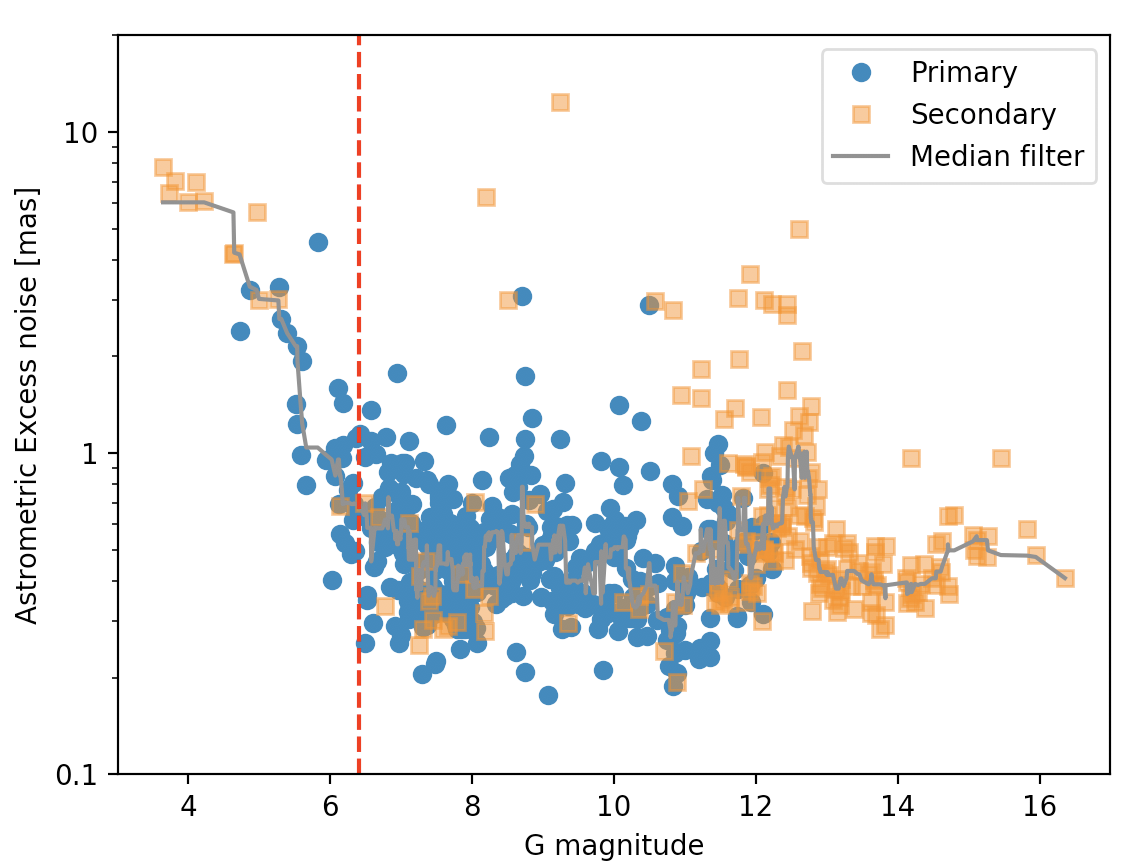
Figure 1: Comparing astrometric excess noise to $G$-magnitude for the 658 stars of Table 3. The red dashed line shows the $G$=6.4 limit discussed in the text. We separate targets from the primary dataset (in blue) and from the secondary dataset (orange). The gray line is a moving median filter of the data.

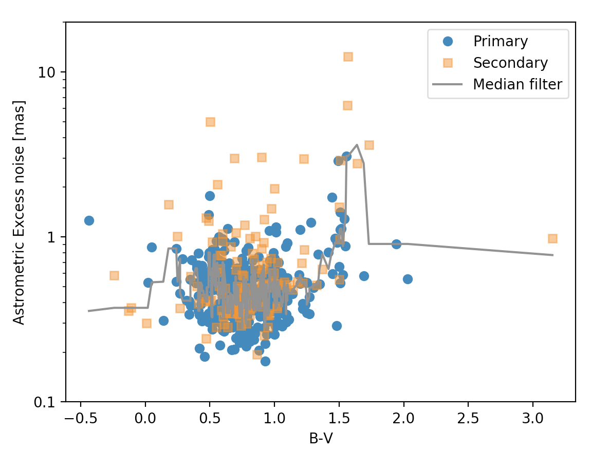
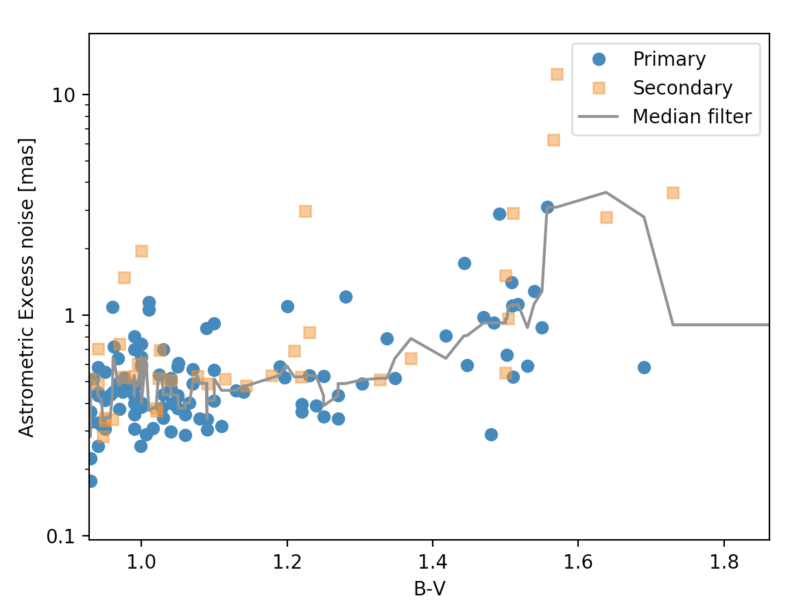
Figure 2: Astrometric excess noise with respect to $B-V$ for 498 sources with $B-V$ measurements and $G$$>$$6.4$. The right panel is a magnification of the region with positive correlation beyond $B-V$=1. Symbols and color are similar to Fig 1.

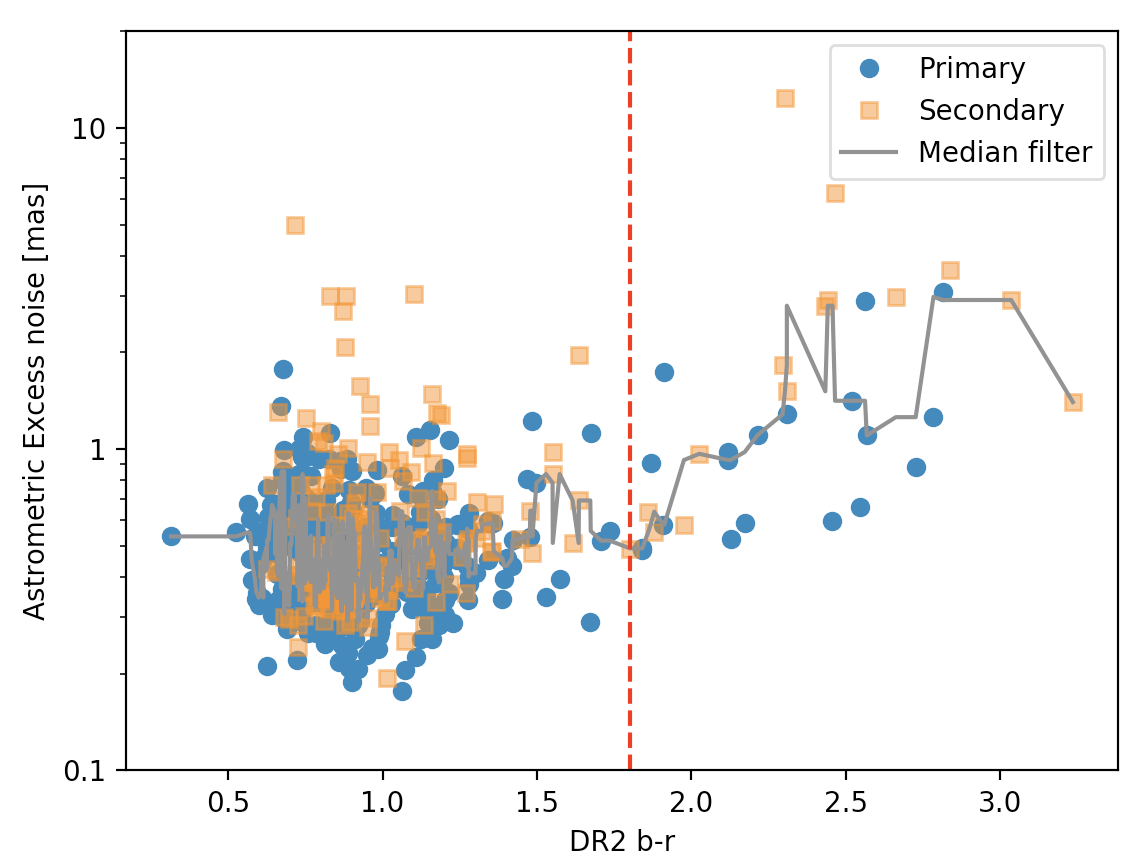
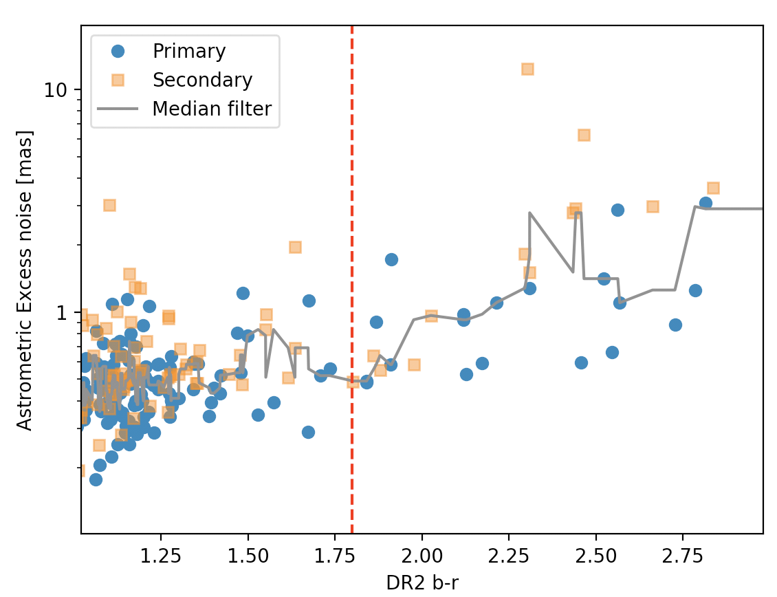
Figure 3: Astrometric excess noise with respect to $b-r$ color index from Gaia DR2 for the 614 sources with $G$$>$$6.4$. The right panel is a magnification of the region with a positive correlation around the limiting color $b-r$=1.8 (red dashed line). Symbols and color are similar to Fig 1.

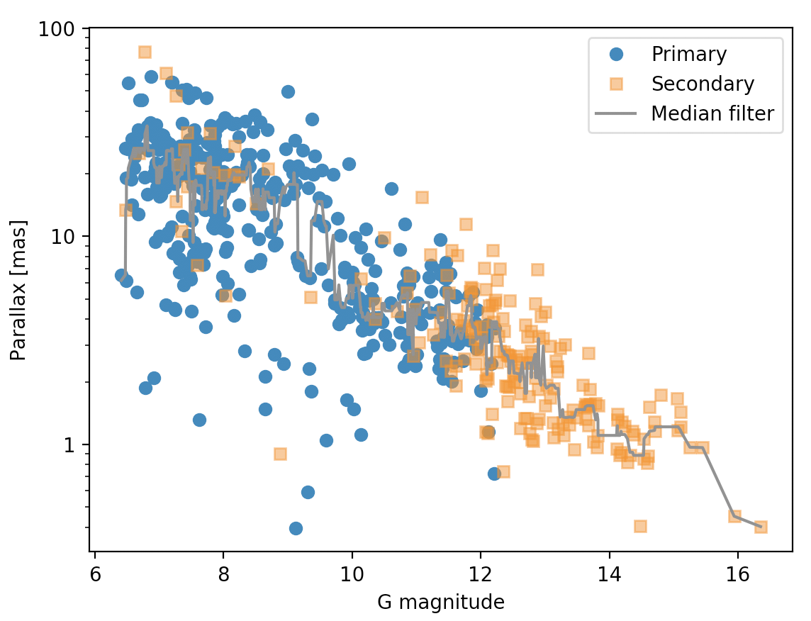
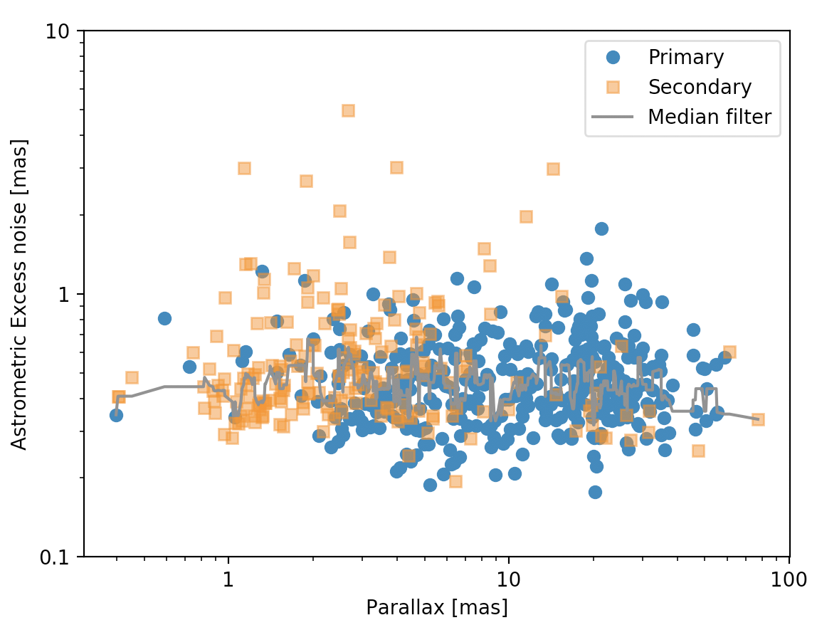
Figure 4: $G$-magnitude with respect to parallax (left-panel) and parallax with respect to astrometric excess noise (right panel) for the 580 sources with $G$$>$$6.4$ and $b-r$$<$$1.8$. Symbols and color are similar to Fig 1.

As can be seen in Fig 1, stars brigher than magnitude 6.4 show a significant drift of increasing excess noise with decreasing magnitude. This is a sign of instrumental systematics (PSF, jitter, CCD sensibility etc.), that are recognised to occur in Gaia data (Lindegren et al. 2018). With $G$-mag$<$6.4, the astrometric excess noise are all larger than 0.4 mas, with a median value about 0.7 mas. In the rest of the paper, we will thus exclude any source with a $G$-mag$<$6.4, reducing the sample to 614 sources.

Moreover, the astrometric excess noise also shows a correlation with color indices, i.e. the B-V as found in Simbad for 498 sources with $G$-mag$>$6.4, and the Gaia DR2 $b-r$ available in the DR2 database for all the 614 sources with $G$-mag$>$6.4, as plotted in Figs 2 and 3. A moving median filter of the data indeed shows a correlation of $\varepsilon_{\text{DR1}}$ with B-V beyond 1, and with DR2 $b-r$ beyond 1.4. The B-V index is not available for all the 614 sources, we thus prefer using the DR2 $b-r$ index as a limiting parameter. As for the magnitude, the astrometric excess noise is larger than 0.4 mas whatever $b-r$ larger than 1.8. A correlation of the along-scan (AL) angle residuals with V-I color was already reported in Section D.2 of Lindegren et al. (2016). These two correlations likely have a common optical origin due to the chromaticity of the star centroid location on the CCD. In the rest of the paper, we will thus also exclude any source with a $b-r$$>$$1.8$, reducing the sample to 580 sources.

Figure 4 shows that the parallax and magnitude are correlated in both primary and secondary datasets, which is not surprising as we expect distant sources to be on average less luminous than sources close-by. Sources of the secondary dataset are located much farther away from the Sun than sources of the primary dataset, which is expected from the absence of Tycho data for the secondary dataset. The astrometric excess noise is not correlated with parallax, but we observe astrometric excess noise measurements on the same order – and even larger – than the parallax for sources of the secondary dataset. This strongly suggests issues with parallax and proper motion modeling, reminding that those parameters are poorly fitted from rough priors in the secondary dataset. We will thus discard from the rest of the study secondary sources for which $\log\pi$$\sim$$\log\varepsilon_{\text{DR1}}$$\pm$$0.5$. We think wiser to postpone their thorough analysis to the future Gaia DR3 release. Moreover, the largest $\varepsilon_{\text{DR1}}$ in the secondary dataset are generally obtained for small parallax ($<$10 mas). This behavior is different from what is observed in the primary dataset where the astrometric excess noise is not correlated with parallax.

The final sample contains 597 planet candidates orbiting around 524 host stars with $G$$>$$6.4$, $b-r$$<$$1.8$, and for sources in the secondary dataset with $\log\pi$-$\log\varepsilon_{\text{DR1}}$¿$0.5$.

3.3 Distribution of astrometric excess noise

In order to get a sense of how $\varepsilon_{\text{DR1}}$ is a relevant quantity to characterize a binary or planetary system, it is crucial to understand how the astrometric excess noise generally varies with respect to the known or unknown inclination of the gravitational systems observed – transiting or not – the presence of a long-period outer companion in the system – presence of RV drift – and the quality of their observations with Gaia – primary or secondary dataset. We perform here an analysis of the distribution of astrometric excess noise of our selected sample of companions and sources as defined in Section 3.2, with respect to following subsets selection criteria:

• Dataset (primary/secondary);

• All planets around the host star are transiting;

• At least one planet is not transiting;

• Detection or hint of an RV drift;

• No hint of an RV drift.

In principle, with orbital inclination fixed to $\sim$90^∘, the semi-major axis of transiting planets host stars should not reach more than a few $\mu$as, and remain undetectable in the DR1 astrometric excess noise. The astrometric scatter is dominated by the instrumental and measurement noises on the order of $\sim$0.6 mas (Lindegren et al. 2016). The distribution of $\varepsilon_{\text{DR1}}$ for transiting planet hosts should be close to the distribution of astrometric scatter due to pure instrumental and measurement noises. On the other hand, system with non-transiting planets allow inclinations down to 0^∘, and host star semi-major axis beyond a few 0.1 mas. We expect their astrometric excess noise to be generally larger than for systems with transiting-only planets. Finally, the detection of a drift in the RV suggest the presence of a hidden outer companion in the system. The astrometric excess noise might be systematically larger for those systems, implying that the astrometric signal is not only due to the companion with a well-defined orbit. This is however certainly not a rule, as shown e.g. in the case of HD 114762 (Kiefer 2019) for which the astrometric excess noise is dominated by the effect of the short period companion HD 114762 Ab.

In Table 4, we present the 10th, 50th and 90th percentiles of the astrometric excess noise distribution according to the different sub-samples defined above. We confront them to the Lindegren et al. (2016) percentiles derived for the whole primary, secondary and Hipparcos DR1 datasets (Tables 1 and 2 in Lindegren et al. 2016) based on more than 1 billion sources observed with Gaia. In Figure 5, we compare in a first panel the distributions of astrometric excess noise for the sources from the primary and secondary datasets with transiting-only planets, and in a second panel, sources from the primary dataset with transiting-only planets to those with at least one non-transiting planet.

The median and 90th percentile value of the $\varepsilon_{\text{DR1}}$ distribution for all subset in the primary dataset are generally compatible with the Lindegren et al. (2016) values. Although Lindegren et al. (2016) study shows that the Hipparcos subset is associated to larger excess noise, Table 4 shows that excluding $G$-mag$>$6.4 and $b-r$$>$$1.8$ objects as proposed in Section 3.1 above leads to decreasing the extent of the astrometric excess noise distribution with values agreeing with the primary dataset. The Hipparcos subset excluding bright and late-type sources is thus likely not different from the full primary dataset.

We observe a clear distinction in the distributions of $\varepsilon_{\text{DR1}}$ between the primary and secondary datasets, with significantly higher astrometric excess noise in the secondary dataset. This could be well explained by the absence, for the secondary dataset, of the Tycho/Hipparcos supplementary positions 24-years in the past that allows deriving robust proper motion and parallax for the sources in the primary dataset. The derivation of proper motion and parallax from Gaia data only with Galactic priors based on magnitude (Michalik et al. 2015b, Lindegren et al. 2016) certainly leads to larger scatter in the residuals of the 5-parameters solution.

Table 4: The distribution of astrometric excess noise with respect to primary, secondary and Hipparcos datasets in the Gaia DR1 database, and varying selection criteria as explained in the text.

Reference of data	DR1 dataset	Subset	$N_{\text{star}}$	Astrometric excess noise
				10th-percentile	Median	90th-percentile
				(mas)	(mas)	(mas)
Lindegren et al. (2016)	primary		2,057,050	0.299	0.478	0.855
(1,142,719,769 stars)	secondary		1,140,662,719	0.000	0.594	2.375
	Hipparcos		93,635	0.347	0.572	1.185
This paper sample (Table 3)	primary		385	0.291	0.451	0.751
(524 stars)		all transiting planets	133	0.271	0.399	0.704
		$>$1 non-transiting planet	252	0.304	0.466	0.786
		with RV drift	46	0.296	0.431	0.633
		no RV drift	339	0.291	0.453	0.761
	secondary		139	0.316	0.423	0.776
		all transiting planets	113	0.336	0.438	0.791
		$>$1 non-transiting planet	26	0.283	0.360	0.701
		with RV drift	7	0.297	0.334	0.511
		no RV drift	132	0.318	0.425	0.794
	Hipparcos		246	0.307	0.466	0.784
		including G$<$6.4 & b-r$>$1.8	297	0.324	0.513	1.048

For transiting sources of the primary dataset, the 90th percentile of the astrometric excess noise distribution is 0.70 mas. This is compatible with, and even lower than, Lindegren et al. (2016) values of the global DR1 solution. For this subset, the 95-th percentile is 0.81 mas, still lower than the 90th-percentile of Lindegren et al. (2016). This generally small astrometric excess noises of the sources with transiting planets is compatible with statistical noise and the non-detection by Gaia of any orbital motion of a star orbited by a planet at short separation ($<$0.1 a.u. or $P$$<$$50$ days) and with an edge-on inclination of its orbit.

The systems in the primary dataset with a non-transiting planet have the highest median among all other subsets (0.47 mas) and the highest 90th percentile (0.78 mas). More importantly, the astrometric excess noise of sources with non-transiting companions is significantly larger than for sources with transiting-only planets. This can also be seen in the lower panel of Figure 5 with a net shift between the two $\varepsilon_{\text{DR1}}$ distributions. This confirms that $\varepsilon_{\text{DR1}}$ contains a non-negligible fraction of astrometric motion for systems with a companion which orbital inclination is not known.

The $\varepsilon_{\text{DR1}}$ in the secondary dataset generally reaches larger values than in the primary dataset, with a 90th percentile for the subset of systems with transiting-only planets $\sim$0.8 mas. This was expected by the less accurate fit of the proper motion and parallax in the secondary dataset compared to the primary. However, this is also much smaller than the 2.3 mas 90th-percentile derived for the whole secondary dataset in Lindegren et al. (2016). Therefore once cleaned from problematic systems, in particular those with $\log\pi/\varepsilon_{\text{DR1}}$$>$$0.5$ (Section 3.2), the astrometric excess noise of remaining objects in the secondary dataset seems robust, with parallax and proper motion most likely well determined (although not published in the DR1).

Interestingly, we find no correlation of the astrometric excess noise distribution with the presence of any drift in the RV data, and even smaller values than in the other subsets. This could be due to the smaller number of sources in this category, which if following a inclination probability density function $\sim\sin I_{c}$ would preferentially have inclinations close to 90^∘, and thus smaller astometric motion. It also suggests that the presence of an outer companion does not have a strong effect on the astrometric excess noise compared to the enhanced astrometric motion due to a small inclination of a non-transiting companion.

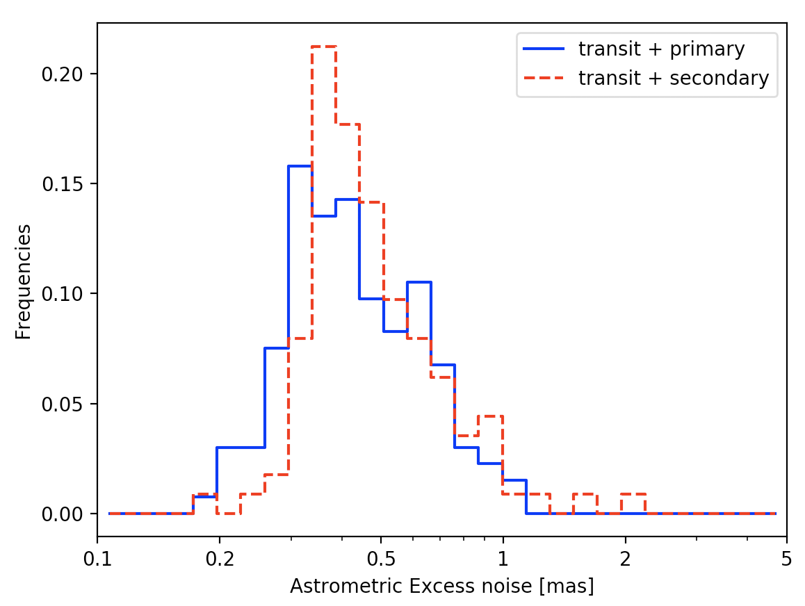
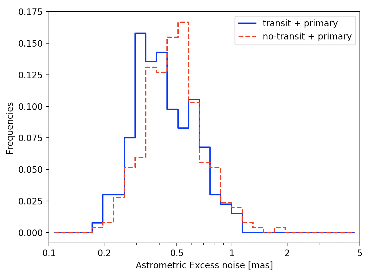
Figure 5: Top panel: the astrometric excess noise distribution for sources with only transiting planets, comparing primary and secondary dataset. Bottom panel: comparing ’only transiting’ and ’non-transiting’ subsets within the primary dataset.

3.4 Testing the noise model

From the 133 and 113 stars with transiting-only planets from the primary and secondary datasets we can test the model of noise used in the simulations of GASTON. In previous studies (Kiefer et al. 2019, Kiefer 2019), we chose to use values based on published estimations of the measurement uncertainty and of the typical external noise (including modeling noise and instrument jitter), respectively $\sigma_{\text{AL}}$=0.4 mas (Michalik et al. 2015a) and $\sigma_{\text{syst}}$=0.5 mas (Lindegren et al. 2016). As we showed in the preceding section, the sources with transiting companion must be generally more similar to sources with no astrometric motion. Therefore, the astrometric excess noise measured by Gaia for these sources should be close to purely instrumental and photonic stochastic scatter.

The distribution of $\varepsilon_{\text{DR1}}$ for these 300 sources from primary and secondary datasets is plotted in Fig. 6. It is compared to simulations of astrometric excess noise of sources with no orbital motion, in the framework of different noise models. We assumed for each simulation random numbers of FoV transits ($N_{\text{FoV}}$) and numbers of measurements per FoV transit ($N_{\text{AL}}$) in the same ranges as those of the sample presented here, e.g. $N_{\text{FoV}}$=15$\pm$8 and $N_{\text{AL}}$=7$\pm$2 with Gaussian distribution, and imposing that $48$$>$$N_{\text{FoV}}$$>$$5$ and $9$$>$$N_{\text{AL}}$$>$$2$. We singled out 5 different noise models of ($\sigma_{\text{syst}}$,$\sigma_{\text{AL}}$), either based on literature values, or based on the best fit of a bi-uniform distribution of $\sigma_{\text{syst}}$ with a fixed median to the $\varepsilon_{\text{DR1}}$ cumulative density function (cdf):

• The constant model for the primary dataset, as used in Kiefer et al. 2019 & Kiefer 2019: $\sigma_{\text{AL}}$=0.4 mas from Michalik et al. (2015a), and $\sigma_{\text{syst}}$=0.5 mas (based on Lindegren et al. 2016),

• A different constant model for the secondary dataset: $\sigma_{\text{AL}}$=0.4 mas as above, and $\sigma_{\text{syst}}$=0.6 mas (based on Lindegren et al. 2016),

• Random $\sigma_{\text{syst}}$ from a distribution with a median at 0.4 mas, uniform from 0.36 to 0.40 mas and from 0.4 to 0.7 mas for the primary dataset,

• Random $\sigma_{\text{syst}}$ from a distribution with a median at 0.45 mas, uniform from 0.4 to 0.45 mas and from 0.45 to 0.8 mas for the secondary dataset,

• Smaller AL angle measurement uncertainty as suggested from Lindegren et al. (2018): $\sigma_{\text{AL}}$=0.1 mas.

The bi-uniform distributions models were found to lead to the best least square fit of the observed $\varepsilon_{\text{DR1}}$ cdf. All 5 models are compared to the data in Figure 6. A model with a wide range of systematic noise better explain the observed distributions for values of astrometric excess noise assumed to be compatible with pure stochastic and systematic noise, e.g. below 0.85 mas and 2.3 mas for sources in the primary and secondary datasets respectively. The constant noise model tends to overestimate the astrometric excess noise, and the simulated distribution decreases too steeply at values closer to 1 mas. The noise $\sigma_{\text{syst}}$ taken from a bi-uniform distribution of values within bounds (e.g. 0.36-0.7 mas in the primary dataset) explains better the full distribution of observed astrometric excess noises. The distribution is damped beyond about 0.85-1 mas for the primary dataset and $\sim$1.2-1.4 mas in the secondary dataset, with less than 1% of the simulations beyond.

We can exclude that the $\sigma_{\text{syst}}$ is much larger than 0.7 mas in the primary dataset, and 0.8 mas in the secondary dataset, since that would extend the core of the distribution towards larger excess noise, therefore leading to a poorer agreement. Finally, we observe that the AL angle measurement uncertainty $\sigma_{\text{AL}}$ does not have a strong impact on the astrometric excess noise. We tested two values, a small uncertainty 0.1 mas, as given in Lindegren et al. (2018), and a more conservative value as assumed by Michalik et al. (2015) of 0.4 mas that corresponds well to the typical AL residuals reported in Lindegren et al. (2016) of 0.65 mas ($\sqrt{(\sigma_{\text{AL}}=0.4)^{2}+(\sigma_{\text{syst}}=0.5)^{2}}$=0.64 mas). We thus fix $\sigma_{\text{AL}}$ to 0.4 mas.

In conclusion, the systematic noise is typically about 0.5 and 0.6 mas respectively in the primary and secondary dataset. But it is likely that for an individual observed source, $\sigma_{\text{syst}}$ can be somewhat larger or smaller by a few fraction of mas. We thus adopt a random systematic noise for each simulation in GASTON uniformly distributed on both sides of the median at 0.4 mas down to 0.36 mas and up to 0.7 mas for sources in the primary dataset, and about the median at 0.45 mas down to 0.4 mas and up to 0.8 mas for sources in the secondary dataset.

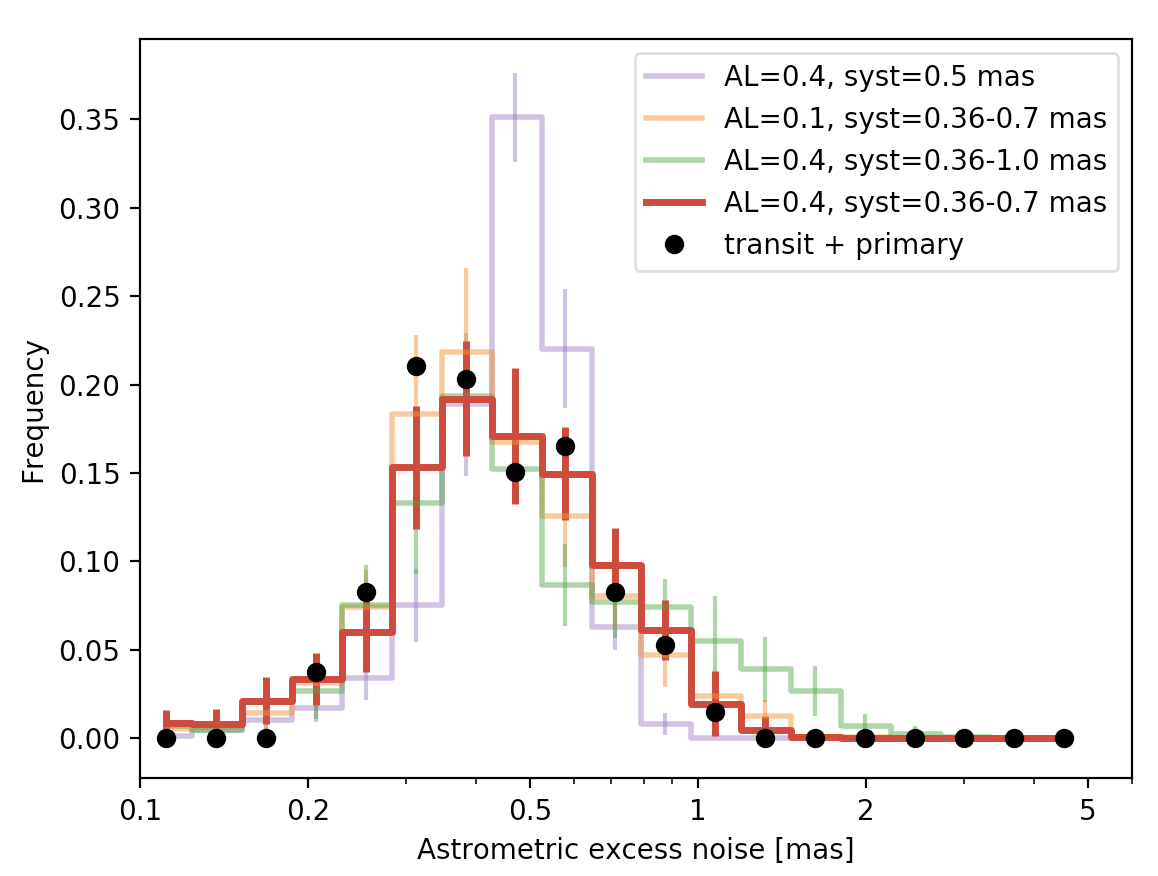
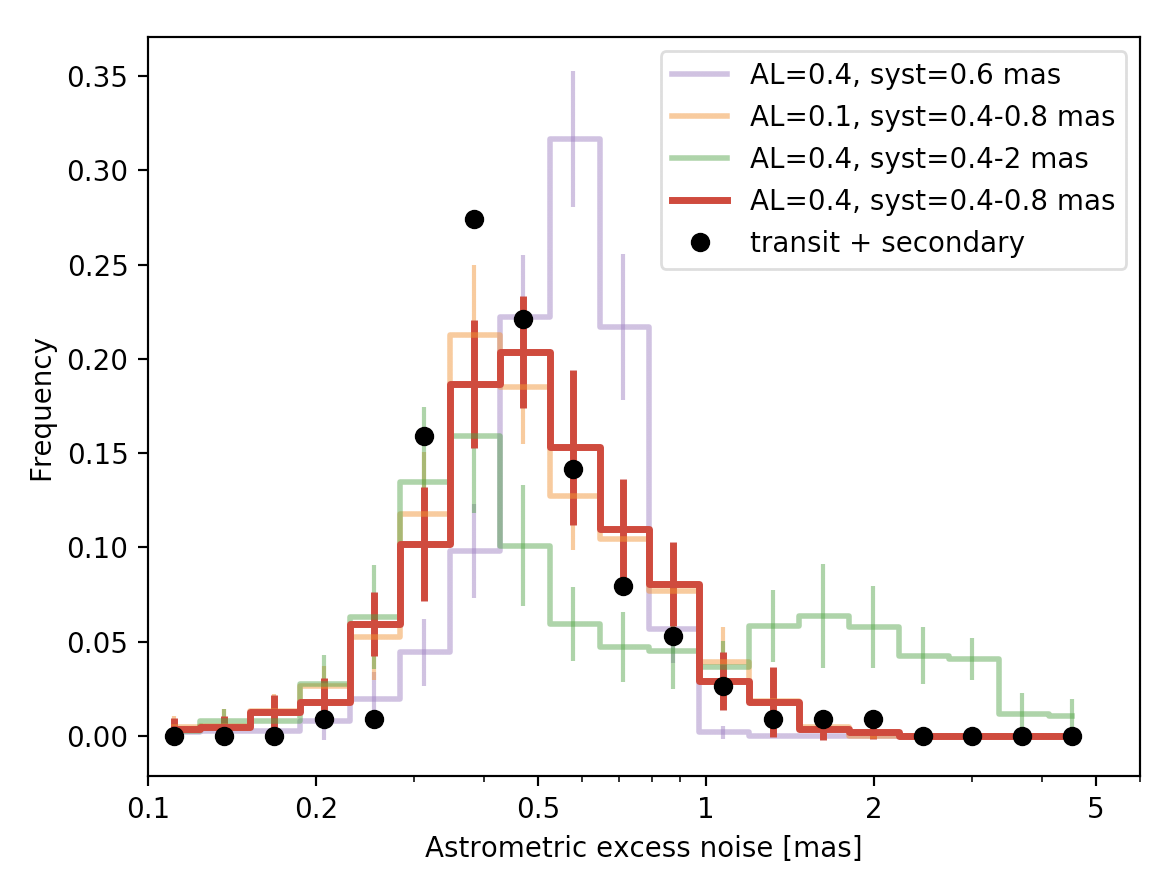
Figure 6: Comparing measurement and systematical noise models to the distribution of astrometric excess noise measurement for sources with transiting companion in the primary dataset (top-panel) and in the secondary dataset (bottom-panel). See text for explanations.

3.5 Detection threshold and source selection

GASTON cannot be used to characterize the mass of as much as 597 planet candidates. This would require several weeks of calculation, while many of them cannot be truly characterized, because the astrometric excess noise is compatible with an edge-on inclination. We thus need to define a robust threshold above which $\varepsilon_{\text{DR1}}$ can be considered significantly non-stochastic – and thus astrophysical – and below which it could be explained by pure stochastic noise.

Given that close to 40-50% of the sources in the Milky Way are part of binary systems (Duquennoy & Mayor 1991, Raghavan et al. 2010), a consequent fraction of Gaia sources – possibly more than 10% – could show a detectable astrometric motion. We thus consider using the 90th-percentiles of Lindegren et al. (2016) based on a sample of more than 1 billion stars, as a detection threshold, above which a significant fraction of $\varepsilon_{\text{DR1}}$ could be imputed to astrometric motion. This was assumed in previous work (Kiefer 2019), but the astrometric excess noise distribution of the present sample might differ from the sample upon which these percentiles were calculated.

In Sections 3.3 and 3.4, we showed that the 90th-percentile of 0.85 mas in the primary sample, as derived in Lindegren et al. (2016) is robust, but the 2.3 mas threshold for secondary dataset sources is excessive and could be more reasonably lowered to $\sim$1.2 mas. This overestimation of the 90th-percentile in Lindegren et al. (2016) must be due to the inclusion of small magnitude, large $b-r$ color sources and badly modelled parallax, which we did clean out from our sample. We will thus use the detections thresholds $\epsilon_{thresh,prim}$=0.85 mas, and $\epsilon_{thresh,sec}$=1.2 mas, above which the astrometric excess noise would be mainly due to supplementary astrometric motion. This reduces our sample to 28 sources (29 planet candidates) with an astrometric detection by Gaia in the DR1. They are the best candidates for orbit inclination and true mass measurement of the companion. They constitutes the ’detection sample’.

We counted 312 non-transiting planet candidates (around 254 sources) for which the inclination is not constrained from photometry and for which the astrometric motion of their host star leads to an astrometric excess noise smaller than the threshold. Even though compatible with pure noise, the astrometric excess noise allow constraining the true astrometric extent of the star’s orbit. This leads to deriving a minimum inclination and a maximum true mass of the exoplanet candidates beyond which they are not compatible with a non-detection. In this sample, we exclude the so-called ’duplicate sources’ in the Gaia DR1, because, for such target, possibly large sets of astrometric measurements are attributed to another source with another ID, and thus lead to underestimate its AL-angle residuals and its astrometric excess noise. This will be of crucial importance if the mass of a companion is found to be smaller than 13.5 M${}_{\text{J}}$. A larger astrometric excess noise leads to a larger mass range. We thus focus on the 227 non-duplicate companions orbiting 187 sources which will constitute the ’non-detection sample’.

The complete list of 29 detected exoplanet candidates is presented in Table 5, and the list of 312 non-detected non-transiting planet candidates is given in Appendix B. Table 6 summarizes all source selection steps applied from Section 2 up to the present section.

Table 5: List of the 29 selected planets which astrometric excess noise overpass the detection threshold (see text). Where uncertainties are missing we will assume 10% errors on the corresponding parameter. The parallax with uncertainties are all taken from the DR1, while those without uncertainties are taken from SIMBAD. We expand this table on-line to also include the 227 exoplanet candidates for which the astrometric excess noise is smaller than the threshold (see Table 6).

RV data

Gaia DR1 data

Name

$P$

$m\sin i$

$K$

$e$

$\omega$

$T_{p}$

$M_{\star}$

$a_{p}$

$\pi$

$a_{\star}\sin i$

Transit

Drift

$\varepsilon_{\text{DR1}}$

$N_{\text{pts}}$

$N_{\text{FoV}}$

Gaia

Duplicate

(days)

(M${}_{\text{J}}$)

(m s-1)

(∘)

-2,450,000

($M_{\odot}$)

(au)

(mas)

(mas)

flag

flag

(mas)

dataset

source

30 Ari B b

335.1$\pm$2.5

9.88$\pm$0.98

272$\pm$24

0.289$\pm$0.092

307$\pm$18

4538$\pm$20

1.160$\pm$0.040

0.992$\pm$0.012

21.42$\pm$0.60

0.173$\pm$0.019

n

n

1.8

71

10

1

n

HAT-P-21 b

4.1244810$\pm$0.0000070

4.07$\pm$0.17

548$\pm$14

0.228$\pm$0.016

309.0$\pm$3.0

4995.014$\pm$0.046

0.947$\pm$0.042

0.04943$\pm$0.00073

3.73$\pm$0.51

0.00076$\pm$0.00011

n

n

0.92

84

10

1

n

HD 114762 b

83.9151$\pm$0.0030

11.64$\pm$0.78

612.5$\pm$3.5

0.3354$\pm$0.0048

201.3$\pm$1.0

-110.89$\pm$0.19

0.895$\pm$0.089

0.361$\pm$0.012

25.88$\pm$0.46

0.116$\pm$0.015

n

n

1.1

130

23

1

n

HD 132563 B b

1544$\pm$34

1.49$\pm$0.14

26.7$\pm$2.2

0.220$\pm$0.090

158$\pm$35

2593$\pm$148

1.010$\pm$0.010

2.623$\pm$0.039

9.30$\pm$0.33

0.0344$\pm$0.0034

n

n

0.85

130

19

1

y

HD 141937 b

653.2$\pm$1.2

9.48$\pm$0.41

234.5$\pm$6.4

0.410$\pm$0.010

187.72$\pm$0.80

1847.4$\pm$2.0

1.048$\pm$0.037

1.497$\pm$0.018

30.62$\pm$0.35

0.396$\pm$0.023

n

n

0.93

236

32

1

y

HD 148427 b

331.5$\pm$3.0

1.144$\pm$0.092

27.7$\pm$2.0

0.160$\pm$0.080

277$\pm$68

3991$\pm$15

1.360$\pm$0.060

1.039$\pm$0.017

14.17$\pm$0.42

0.0118$\pm$0.0012

n

n

1.1

131

17

1

n

HD 154857 b

408.60$\pm$0.50

2.248$\pm$0.092

48.3$\pm$1.0

0.460$\pm$0.020

57.0$\pm$4.0

3572.5$\pm$2.4

1.718$\pm$0.026

1.2907$\pm$0.0066

15.56$\pm$0.39

0.0251$\pm$0.0013

n

n

0.93

122

19

1

n

HD 154857 c

3452$\pm$105

2.58$\pm$0.15

24.2$\pm$1.1

0.060$\pm$0.050

352$\pm$37

5219$\pm$375

1.718$\pm$0.026

5.35$\pm$0.11

15.56$\pm$0.39

0.1194$\pm$0.0081

n

n

0.93

122

19

1

n

HD 164595 b

40.00$\pm$0.24

0.0508$\pm$0.0070

3.05$\pm$0.41

0.088$\pm$0.093

145$\pm$135

6280$\pm$12

0.990$\pm$0.030

0.2281$\pm$0.0025

35.11$\pm$0.38

0.000392$\pm$0.000056

n

n

0.93

62

8

1

y

HD 16760 b

465.1$\pm$2.3

13.29$\pm$0.61

408.0$\pm$7.0

0.067$\pm$0.010

232$\pm$10

4723$\pm$12

0.780$\pm$0.050

1.081$\pm$0.023

14

0.25

n

n

3.0

62

10

2

n

HD 177830 b

410.1$\pm$2.2

1.320$\pm$0.085

32.64$\pm$0.98

0.096$\pm$0.048

189

254$\pm$49

1.17$\pm$0.10

1.138$\pm$0.033

15.94$\pm$0.37

0.0195$\pm$0.0022

n

n

0.87

89

19

1

n

HD 185269 b

6.8379$\pm$0.0010

0.954$\pm$0.069

90.7$\pm$4.4

0.296$\pm$0.040

172$\pm$11

3154.089$\pm$0.040

1.28$\pm$0.10

0.0766$\pm$0.0020

19.10$\pm$0.41

0.00104$\pm$0.00012

n

n

0.97

74

16

1

n

HD 190228 b

1136.1$\pm$9.9

5.94$\pm$0.30

91.4$\pm$3.0

0.531$\pm$0.028

101.2$\pm$2.1

3522$\pm$12

1.821$\pm$0.046

2.602$\pm$0.027

15.77$\pm$0.34

0.1278$\pm$0.0079

n

n

0.86

116

16

1

y

HD 197037 b

1036$\pm$13

0.807$\pm$0.060

15.5$\pm$1.0

0.220$\pm$0.070

298$\pm$26

1353$\pm$86

1.1

2.1

30.01$\pm$0.32

0.043

n

n

0.99

107

17

1

n

HD 4203 b

431.88$\pm$0.85

2.08$\pm$0.12

60.3$\pm$2.2

0.519$\pm$0.027

329.1$\pm$3.0

1918.9$\pm$2.7

1.130$\pm$0.064

1.165$\pm$0.022

12.67$\pm$0.44

0.0259$\pm$0.0023

n

n

0.85

60

11

1

n

HD 5388 b

777.0$\pm$4.0

1.97$\pm$0.10

41.7$\pm$1.6

0.400$\pm$0.020

324.0$\pm$4.0

4570.0$\pm$9.0

1.2

1.8

18.86$\pm$0.32

0.052

n

n

1.4

327

48

1

y

HD 6718 b

2496$\pm$176

1.56$\pm$0.12

24.1$\pm$1.5

0.100$\pm$0.075

286$\pm$50

4357$\pm$251

0.96

3.6

19.74$\pm$0.41

0.11

n

n

1.1

199

29

1

y

HD 7449 b

1275$\pm$13

1.31$\pm$0.52

42$\pm$15

0.820$\pm$0.060

339.0$\pm$6.0

5298$\pm$26

1.1

2.3

27.14$\pm$0.41

0.076

n

n

0.94

61

12

1

y

HD 95127 b

482.0$\pm$5.0

5.04$\pm$0.82

116$\pm$12

0.11$\pm$0.10

40$\pm$38

3200$\pm$50

1.20$\pm$0.22

1.278$\pm$0.079

1.31$\pm$0.58

0.0067$\pm$0.0034

n

n

1.2

41

8

1

n

HD 96127 b

647$\pm$17

4.01$\pm$0.85

105$\pm$11

0.30$\pm$0.10

162$\pm$18

3969$\pm$31

0.91$\pm$0.25

1.42$\pm$0.13

1.87$\pm$0.83

0.0112$\pm$0.0064

n

n

1.1

109

16

1

n

HIP 65891 b

1084$\pm$23

6.00$\pm$0.41

64.9$\pm$2.4

0.130$\pm$0.050

356$\pm$16

6015$\pm$49

2.50$\pm$0.21

2.804$\pm$0.088

6.53$\pm$0.37

0.0420$\pm$0.0053

n

n

1.1

237

35

1

n

K2-110 b

13.86375$\pm$0.00026

0.053$\pm$0.011

5.5$\pm$1.1

0.079$\pm$0.070

90$\pm$122

6863

0.738$\pm$0.018

0.10207$\pm$0.00083

8.6

0.000060

n

n

1.3

54

9

2

y

K2-34 b

2.9956290$\pm$0.0000060

1.683$\pm$0.061

207.0$\pm$3.0

0.000$\pm$0.027

90

7144.347030$\pm$0.000080

1.226$\pm$0.052

0.04353$\pm$0.00062

3.28$\pm$0.68

0.000187$\pm$0.000040

n

n

1.00

117

16

1

y

WASP-11 b

3.7224650$\pm$0.0000070

0.540$\pm$0.052

82.1$\pm$7.4

0

90

4473.05588$\pm$0.00020

0.800$\pm$0.025

0.04364$\pm$0.00045

7.49$\pm$0.58

0.000211$\pm$0.000027

n

n

1.1

60

10

1

n

WASP-131 b

5.3220230$\pm$0.0000050

0.272$\pm$0.018

30.5$\pm$1.7

0

90

6919.82360$\pm$0.00040

1.060$\pm$0.060

0.0608$\pm$0.0011

4.55$\pm$0.56

0.000068$\pm$0.000010

n

n

0.95

53

7

1

n

WASP-156 b

3.8361690$\pm$0.0000030

0.1305$\pm$0.0087

19.0$\pm$1.0

0.0000$\pm$0.0035

90

4677.7070$\pm$0.0020

0.842$\pm$0.052

0.04529$\pm$0.00093

8.2

0.000055

n

n

1.5

38

7

2

n

WASP-157 b

3.9516205$\pm$0.0000040

0.559$\pm$0.049

61.6$\pm$3.8

0.000$\pm$0.055

90

7257.803194$\pm$0.000088

1.26$\pm$0.12

0.0528$\pm$0.0017

3.76$\pm$0.66

0.000084$\pm$0.000019

n

n

0.87

69

9

1

n

WASP-17 b

3.7354330$\pm$0.0000076

0.508$\pm$0.030

59.2$\pm$2.9

0

90

4559.18096$\pm$0.00023

1.190$\pm$0.030

0.04993$\pm$0.00042

2.57$\pm$0.31

0.0000523$\pm$0.0000072

n

n

0.85

202

25

1

n

WASP-43 b

0.8134750$\pm$0.0000010

1.76$\pm$0.10

550.3$\pm$6.7

0

90

5528.86774$\pm$0.00014

0.580$\pm$0.050

0.01422$\pm$0.00041

11

0.00047

n

n

2.0

63

7

2

n

Table 6: Number of sources and planets in our sample after the several selection criteria introduced in Sections 2, 3.2 and 3.5.

Criterion	Article section	# stellar hosts	# planets
exoplanets.org	2	2466	3262
RV planets	2	782	911
sources in the DR1	3.1	658	755
$G$$>$$6.4$	3.2	614	705
$b-r$$<$$1.8$	3.2	580	654
Separation into primary/secondary Gaia DR1 datasets
primary	3.3	385	442
secondary ; $\log(\pi/\varepsilon_{\text{DR1}})$$>$$0.5$	3.2 ; 3.3	139	154
$\varepsilon_{\text{DR1}}>$ threshold: the detection sample
primary ; $\varepsilon_{\text{DR1}}$$>$$0.85$ mas	3.5	24	25
secondary ; $\varepsilon_{\text{DR1}}$$>$$1.2$ mas	3.5	4	4
$\varepsilon_{\text{DR1}}<$ threshold and non-transiting: the non-detection sample
primary ; $\varepsilon_{\text{DR1}}$$<$$0.85$ mas ; no transit ; non duplicate	3.5	165	201
secondary ; $\varepsilon_{\text{DR1}}$$<$$1.2$ mas ; no transit ; non duplicate	3.5	18	26

4 GASTON simulations and new improvements

4.1 General principle

In the present study, our goal is to constrain the inclination and true mass of RV planet candidates using the released Gaia astrometric data. To do so, we are applying the GASTON method described in Kiefer et al. 2019 & Kiefer 2019. This algorithm simulates the residuals of Gaia’s 5-parameters fit of a source accounting for a supplementary astrometric motion due to a perturbing RV-detected companion. It leads to simulated astrometric excess noise $\varepsilon_{\text{simu}}$ depending on the actual inclination of the RV-detected orbital motion. It also accounts for measurement noise and modeling errors in the reduction of the DR1 through the noise model adopted in Section 3.4. These simulations are then compared to the astrometric excess noise actually measured by Gaia and reported in the DR1 database (Table 3) to derive a matching orbital inclination.

The GASTON algorithm is embedded into an MCMC process, with emcee (Foreman-Mackey et al. 2013), that allows deriving the posterior distributions of orbital inclination and true mass of the RV companion among other parameters. To sum up, the varied physical parameters in the MCMC run are the orbital period $P$, the eccentricity $e$, the longitude of periastron $\omega$, the periastron time of passage $T_{p}$, the inclination $I_{c}$, the minimum mass $m\sin i$, the star mass $M_{\star}$, the parallax $\pi$, an hyper-parameter $f_{\varepsilon}$ to scale error bars on $\varepsilon_{\text{DR1}}^{2}$, and a jitter term $\sigma_{\text{K, jitter}}$. Some of these parameters have strong gaussian priors from RV ($P$, $e$, $T_{p}$, $\omega$, $m\sin i$), or from other analysis ($M_{\star}$, $\pi$). The hyper-parameter $f_{\varepsilon}$ follows a Gaussian prior about 0 with a standard deviation of 0.1. The jitter term follows a flat prior between 0 and $\sqrt{3}$ assuming that the published uncertainty on $K$ could be underestimated by as much as a factor $\sqrt{1+\sigma_{\text{K, jitter}}^{2}}$=2. Generally, we adopt a $\text{d}p(I_{c})$=$\sin I_{c}\text{d}I_{c}$ prior probability distribution for the inclination, assuming the inclination of orbits among RV-candidates is isotropic. If the MCMC converges to an inclination strongly different from 90^∘ despite the low prior probability, that implies the data inputs have a significant weight in the likelihood.

4.2 Dealing with proper motion and parallax in the simulations

For sources in the primary dataset, we assume that the proper motion fit as performed by Gaia in the DR1 is disentangled from the hidden astrometric orbit. We thus assume that the astrometric excess noise is purely composed of noise and orbital motion, and that it is not needed to fit out excess parallax and proper motion to the simulated astrometric orbit. This is justified by the addition of past Hipparcos or Tycho-2 positions in the Gaia’s reduction for fitting proper motion of primary dataset sources, thus based on astrometric measurements spanning more than 24 years. Given that the orbital periods of all studied companions are smaller than 14 years, the fit of proper motion to the simulated orbits reduces the amplitude of the simulated residuals – and thus of the astrometric excess noise – only by a small amount. Numerical simulations show that in the worst case scenario with a Tycho-2 position uncertainty of $\sim$100 mas, the average simulated astrometric excess noise $\varepsilon_{\text{simu}}$ is lowered by less than 0.2 mas. This offset reduces to less than 0.05 mas if a Hipparcos position ($\sigma_{\text{RA,DEC}}$$\sim$$1$ mas) is used instead or if $P$$<$$10$ days. Hipparcos positions are available for 171 over the 190 primary sources in our sample, while only 6 sources have a Tycho-2 position with more than 20 mas of uncertainty and a companion with $P$$>$$10$ days. These 6 sources, HD 95872, NGC 2423 3, BD+20 2457, HD 233604, BD+15 2375, and M67 SAND 364, all belongs to the non-detection sample. For those, the astrometric excess noise that we simulate with GASTON for a given companion orbit and at a given orbital inclination could be overestimated by up to $\sim$0.2 mas. Thus GASTON possibly underestimates the upper-limit on the companion true mass for those stars.

For sources in the secondary dataset, the proper motion given in the DR1 is derived from the Gaia data only, without a supplementary data point from Tycho-2 or Hipparcos. An important part of the orbital motion could thus be mistaken for proper motion during the Gaia data reduction of the DR1, especially for orbital periods at which the Gaia measurements along the 416-days time baseline of the DR1 campaign could appear almost linear. For sources from the secondary dataset, we thus perform a fit of linear motion to the simulated astrometric orbit, from which residuals we derive $\varepsilon_{\text{simu}}$.

For sources of both datasets, fitting the parallax to the astrometric orbit does not have a significant effect on $\varepsilon_{\text{simu}}$ even if $P$$\sim$$365$ days and if the orbital and parallax motions are aligned. Numerical tests of parallax fit to simulated data along an astrometric orbit with $P$$\sim$$365$ days and randomizing along the unknown longitude of ascending node, $\Omega$ from 0 to 2$\pi$, leads to a typical reduction of the average $\varepsilon_{\text{simu}}$ smaller than 0.05 mas. Fitting parallax to the simulated astrometric orbit is thus unnecessary, leading to negligible deviations on the simulated astrometric excess noise.

4.3 Recent improvements

Since Kiefer (2019), we have done few improvements, with the list below:

• The number of walkers was reduced from 200 to 20, as it improved the speed of convergence of the MCMC while leading to equivalent results;

• The maximum number of iterations is increased to 1,000,000. The MCMC stops whenever the autocorrelation length of every parameters stops progressing by more than 1% and is at least 50 times smaller than the actual number of iterations;

• The host star and companion magnitude are calculated using a continuous series of model from planetary mass up to stellar mass of 30 M_⊙. We also implemented the reflection of stellar light on the surface of the companion. These issues are discussed in Appendix A.

We highlight here an important effect of the modeling of the light reflected from the companion surface on the motion of the photocenter, and developed in more details in the Appendix. For mass ratios $M_{c}/M_{\star}$$\sim$$10^{-5}-10^{-3}$ and companion orbit semi-major axis $a_{c}$$<$$0.5$ a.u, the companion reflected light can become more important than the star’s emission in the calculation of the photocenter semi-major axis, with $a_{\text{ph}}$=$L_{c}a_{c}+L_{\star}a_{\star}$. The astrometric motion of the system observed from Earth can even follow the motion of the companion itself rather than the motion of the stellar host. This could lead to wrongly determine the orientation (retrograde/prograde) of the primary star orbit, and strongly underestimate the primary star semi-major axis and thus the mass of the companion. This effect cannot be seen in the present study because it is smaller than the adopted detection thresholds (Section 3.5), but should be taken into account in future analysis of Gaia’s time series of systems with planets.

Concerning the definition of the parameters explored in the MCMC corresponding to inclination, eccentricity and longitude $\omega$, they are improved compared to Kiefer (2019), solving singularity issues at the border of the domain expected for these parameters:

• Adopting $\lambda_{I_{c}}$=$\tan(2I_{c}-\pi/2)$ as was used in Kiefer (2019) led the StretchMove algorithm of emcee (Foreman-Mackey et al. 2013) to get stuck in low probability regions with large or small inclinations, much wider in terms of $\lambda_{I_{c}}$. We thus considered instead simply varying $I_{c}$ imposing rigid boundaries at $I_{c}$=0 and $\pi/2$.

• The exploration of the ($e$,$\omega$) space was not optimal, especially around the singularity $e$=0. We thus varied instead $\lambda_{\text{c}}$=$\tan(\frac{\pi}{2}e\cos\omega)$ and $\lambda_{\text{s}}$=$\tan(\frac{\pi}{2}e\sin\omega)$, with $e$ and $\omega$ being then obtained from the simple transformations and combinations of $\lambda_{\text{c}}$ and $\lambda_{\text{s}}$.

4.4 Application of GASTON to the defined samples

We apply GASTON on the 29 candidate exoplanets of the detection sample, orbiting the 28 sources which astrometric excess noise exceed the detection thresholds fixed in Section 3.5 and listed in Table 5. For those, with the star’s orbit a priori detected in the astrometric data, an inclination and true mass could technically be measured.

For the 227 non-transiting companions of the non-detection sample listed in Table LABEL:tab:list_planets_nondet, we also used GASTON to derive the lowest inclination and largest mass possible for the companion, beyond which the astrometric excess noise would become too large to be compatible with $\varepsilon_{\text{DR1}}$. In order to limit the computation time, and since these calculations only leads to parameter ranges and not strict measurements, we reduced the maximum number of MCMC steps in GASTON to 50,000 for these 227 companions. Moreover, conversely to what adopted for the detection sample, for those 227 companions we adopt a flat prior for the inclination. The shape of the prior distribution of the inclination tends to dictate the shape of the posterior distributions if the simulated astrometric excess noise is compatible with $\varepsilon_{\text{DR1}}$ for inclinations of 90${}^{c}irc$ down to $\sim$0^∘. This prior artificially increases the conventional lower limit, such as 3-$\sigma$, for inclination – and thus decreases the upper-limit on mass. This is typically the case for companions in the non-detection sample with $\varepsilon_{\text{DR1}}$ compatible with noise and $a_{\star}\sin i$$\ll$$\varepsilon_{\text{DR1}}$. Adopting a flat prior for the inclination favours instead the likelihood – and thus the data – to dictate the shape of the posterior distributions down to small inclination. This better reveals the variations of the inclination and mass posteriors only due to incompatibilities between the $\varepsilon_{\text{simu}}$ and $\varepsilon_{\text{DR1}}$ at inclinations close to 0^∘.

In the following, we will only report for the resulting posteriors of the inclination $I_{c}$ and its deriving parameters: the true mass of the companion, the photocenter semi-major axis, and the magnitude difference between the companion and its host star.

5 Results

5.1 General results

Out of the results produced by GASTON, we identified 3 possible situations:

• Orbits leading to a firm measurement of the RV orbit inclination and the true mass of the companions. This concerns 9 exoplanet candidates out of 29 in the detection sample. This is summarized in Section 5.2.1;

• Orbits for which the astrometry cannot constrain the inclination. Because of the noise, producing a measured astrometric excess noise compatible with the RV orbital motion is possible for a large range of inclinations. The derived solution follows mainly the $\sin i$ prior distribution of inclination, with a median about 60^∘, 1-$\sigma$ confidence interval within 30-80^∘ and a 3-$\sigma$ (99.85%) percentile larger than 89.5^∘. Only the upper-limit on the mass and the lower-limit on the inclination is informative. This concerns 18 exoplanet candidates from the detection sample and the 227 exoplanet candidates from the non-detection sample. This is summarized in Sections 5.2.2 and  5.3;

• Companions for which the astrometric excess noise could never be reached in the simulations testing any inclinations from 0.001 to 90^∘. The Gaia astrometric excess noise is incompatible with the published RV orbit. Two companions from the detection sample enter this situation, WASP-43 b and WASP-156 b (see Section 5.2.3).

For the 29 companions of the detection sample, the results of GASTON according to different situations introduced above are presented in Tables 8 & 7. Moreover, Table 9 summarizes the parameter limits derived for the 227 companions of the non-detection sample. In both tables, we list the resulting corrected mass, astrometric orbit semi-major axis, estimated magnitude difference between the host and the companion, MCMC acceptance rate and convergence indicator $N_{\text{steps}}/\text{max}(\tau_{\lambda})$ (see below).

The acceptance rate delivered by emcee allows to quantify the probability of reaching $\varepsilon_{\text{DR1}}$ through all simulations performed during the MCMC process. Typically, if an MCMC performs well, the acceptance rate must reach 0.2-0.4. This is the case for all 9 companions entering situation #1, except one, HD 96127 b for which it is 0.06. Low values of the acceptance rate usually imply too large steps in the Monte-Carlo process (Foreman-Mackey et al. 2013). We can firmly exclude any ”steps issue”, since the geometry of the parameter space is the same for all systems, and the steps for the different parameters have been tuned such that well behaved cases fullfill the 0.2-0.4 criterion. Rather we explain this low acceptance rate by the presence of noise in our simulations. A fortuitous pile-up of noise can allow some simulations to be compatible with $\varepsilon_{\text{DR1}}$=1.124 mas even with an inclination close to 90^∘ and a negligible photocenter orbit. With a $\sin i$-prior on inclination favouring the edge-on configuration, this is sufficient to drag the MCMC towards exploring regions where producing such astrometric excess noise is not frequent. The low acceptance rate is a reflection of this low frequency. This leads, in the case of HD 96127 b, to a 3-$\sigma$ upper-limit on the inclination of 89.54^∘. This is the same mechanism that explains the small acceptance rates associated to mass upper-limits for all companions entering situation #2.

The autocorrelation length $\tau_{\lambda}$ probes the quality of a $\lambda$–parameter exploration by the MCMC during a run. With emcee and its Goodman-Weare algorithm (Goodman & Weare 2010) it can be considered that convergence is reached if at least $N_{\text{steps}}/\tau_{\lambda}$$>$$50$ (Foreman-Mackey et al. 2013), and at best if $\delta\tau_{\lambda}/\tau_{\lambda}$$<$$1$% for all parameters $\lambda$. The errors on the estimations of the posteriors are then reduced by a factor smaller than $1/\sqrt{50}$$\sim$$0.14$. Longer chains obviously produce more accurate results, but are also more time consuming. This paper is not aiming perfect accuracy, since only based on a preliminary estimation of one quantity, the astrometric excess noise, by Gaia. We thus decided to stop the MCMC whenever $N_{\text{steps,max}}$ is reached or $N_{\text{steps}}/\text{max}(\tau_{\lambda})$$>$$50$ and $\delta\tau_{\lambda}/\tau_{\lambda}$$<$$1$% for all parameters $\lambda$. With up to 1,000,000 steps and 20 walkers for 10 parameters to explore, the MCMC should have enough time to converge. This allows to identify problematic systems, such as e.g. HD 96127 b, for which the exploration of the parameter space is inefficient. In Table 8, we identify 3 companions – including HD 96127 b – for which GASTON did not converge after $N_{\text{step}}$=1,000,000 iterations, with a maximum autocorrelation length larger than $N_{\text{step}}/50$ and a small acceptance rate. The posteriors for those companions cannot be reliable, and the width of the confidence intervals on their mass is most likely underestimated.

5.2 Detection sample

5.2.1 SItuation #1: mass measurement for 2 possible massive exoplanets, 2 BDs and 5 M-dwarfs

We illustrates this first case scenario in Figure 7 with the example of 30 Ari B b for which with a period of 335 days, the astrometric excess noise of 1.78 mas leads to an inclination of $4.14$^∘${}_{-0.90}^{+0.96}$ and a corrected mass of $148_{-27}^{+42}$ M${}_{\text{J}}$ instead of an $m\sin i$=10$\pm$1 M${}_{\text{J}}$. The top panel of Fig. 7 shows the simulated astrometric excess noise obtained for 10,000 different values of inclinations from 0.001 to 90^∘. For any inclinations below 1^∘ the true mass of 30 Ari B b is too large and the magnitude difference with the primary star is smaller than 2.5; these simulations are ignored since they would imply the presence of a detectable secondary component in the spectrum of this system, conversely to what observed. The bottom panel of Fig. 7 compares the $I_{c}$ posterior distribution – probability density function or PDF – to the PDF of an ensemble of same size drawn from the assumed prior density function, d$p$=$\sin I_{c}$d$I_{c}$. This posterior PDF is well distinct from the prior PDF which thus have a minor impact on the posterior distributions output from the MCMC. The corner plot of all posterior distributions for 30 Ari B b is shown in Figure 8.

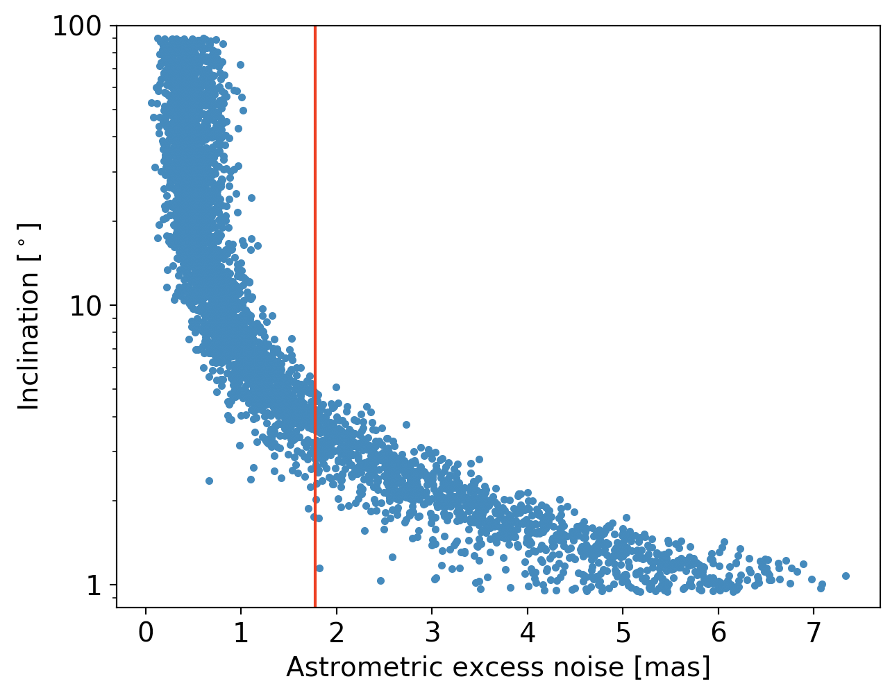
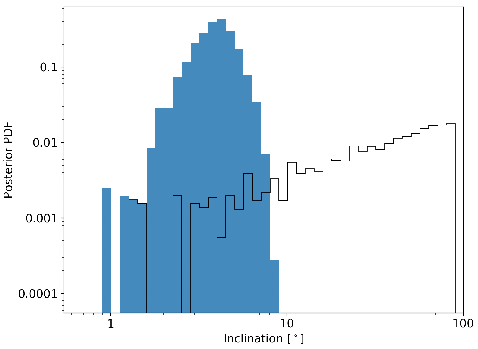
Figure 7: Examples of situation #1 with 30 Ari B b, primary dataset, $P$=335 days, $a_{\star}\sin i$=0.17 mas and $\varepsilon_{\text{DR1}}$=1.78 mas. Top-panel: $I_{c}$ plotted against the derived $\varepsilon_{\text{simu}}$ for every simulations (blue points). The red line shows $\varepsilon_{\text{DR1}}$. Bottom-panel: the $I_{c}$ posterior probability density function (PDF) in blue, compared to the $\sin I_{c}$ prior PDF (black solid line).

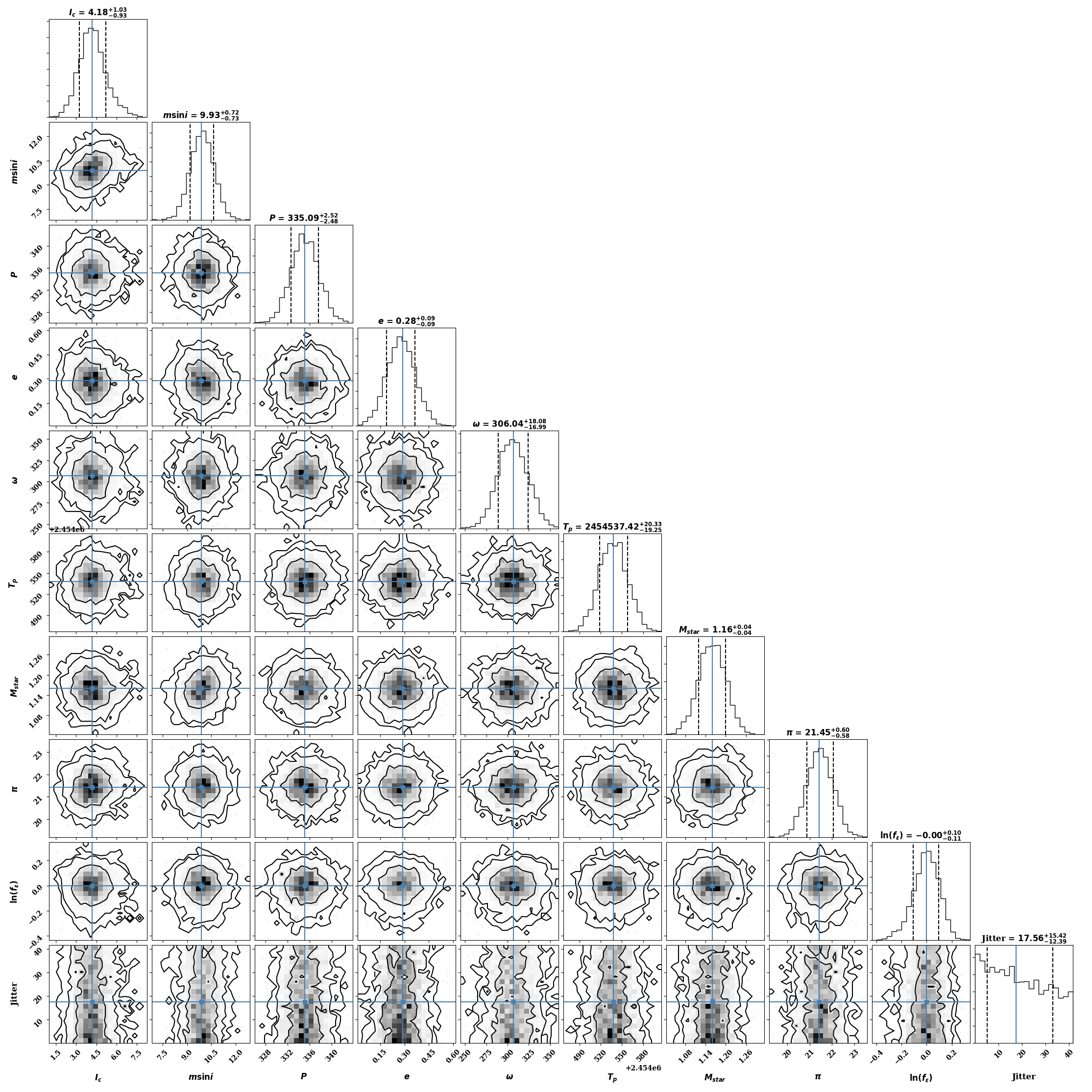
Figure 8: Corner plot of posterior distributions for all explored parameters with the MCMC for 30 Ari B b from situation #1 (Section 5.2.1).

In this category, all other GASTON runs work similarly as well as 30 Ari B b, with the exception of HD 96127 b which MCMC run could not converge after 1,000,000 iterations. In total, the true masses for 9 exoplanet candidates could be determined using GASTON, with 8 orbiting sources from the primary dataset and one, HD 16760 b, from the secondary dataset. We determined that 7 of the companions are not planets, and two, could be likely brown-dwarf or M-dwarf, but the planetary nature cannot be excluded at 3-$\sigma$.

Among the primary sources, we find that HD 5388 b, HD 6718 b, HD 114762 b and HD 148427 b are constrained within the brown dwarf/M-dwarf domain with the 3-$\sigma$ mass-ranges, respectively (57, 150) M${}_{\text{J}}$, (29, 157) M${}_{\text{J}}$, (33, 328) M${}_{\text{J}}$ and (27, 345) M${}_{\text{J}}$. We found moreover that 30 Ari B b and HIP 65891 b are stars in the M-dwarfs mass regime with masses larger than 80 M${}_{\text{J}}$.

The two possible planets are HD 141937 b and HD 96127 b. The true mass of HD 141937 b is located just beyond the boundary between massive planets and low-mass brown dwarfs with $M$=27.5${}^{+6.9}_{-10.8}$ M${}_{\text{J}}$ at 1-$\sigma$ but a mass possibly as low as $9$ M${}_{\text{J}}$ at 3-$\sigma$.

The true mass of HD 96127 b is most likely well within the stellar domain with $M$=190${}^{+284}_{-184}$ M${}_{\text{J}}$ and an inclination $I_{c}$=1.364${}^{+38.527}_{-0.763}$ ​^∘ at 1-$\sigma$. Within the 1-$\sigma$ confidence interval, a true mass of HD 96127 b as low as 6 M${}_{\text{J}}$ could also be compatible with $\varepsilon_{\text{DR1}}$. However, we already noted that GASTON did not converge for this precise case, due to a marginal but possible compatibility of the Gaia DR1 astrometry with an edge-on configuration, as revealed by the low 0.05 acceptance ratio of the MCMC run. The $1$-$\sigma$ bounds of HD 96127 b’s mass are thus questionable and its true nature is still uncertain.

The results for the single source from the Gaia DR1’s secondary dataset within situation #1, HD 16760 b, are given in table 8, and illustrated in Fig. 9. HD 16760 b (Bouchy et al. 2009), is the first companion with a possible planetary mass discovered with the SOPHIE spectrograph (Perruchot et al. 2013) actually is not a planet. With a parallax of 14 mas and an astrometric excess noise of 2.99 mas, we found its astrometry to be rather compatible with an M-dwarf which true mass is larger than 13.5 M${}_{\text{J}}$ at 3-$\sigma$.

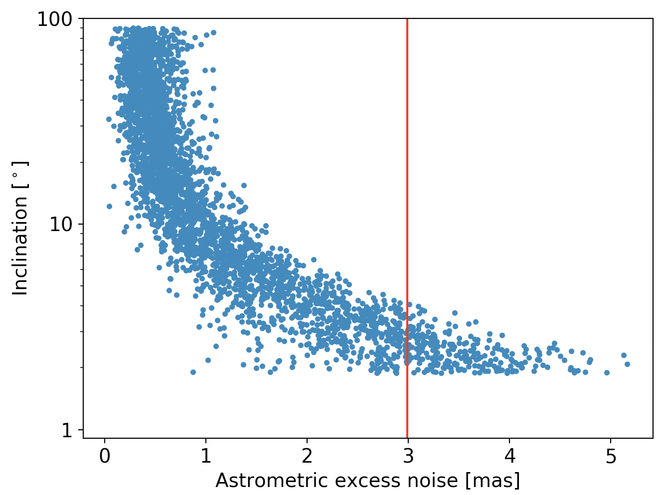
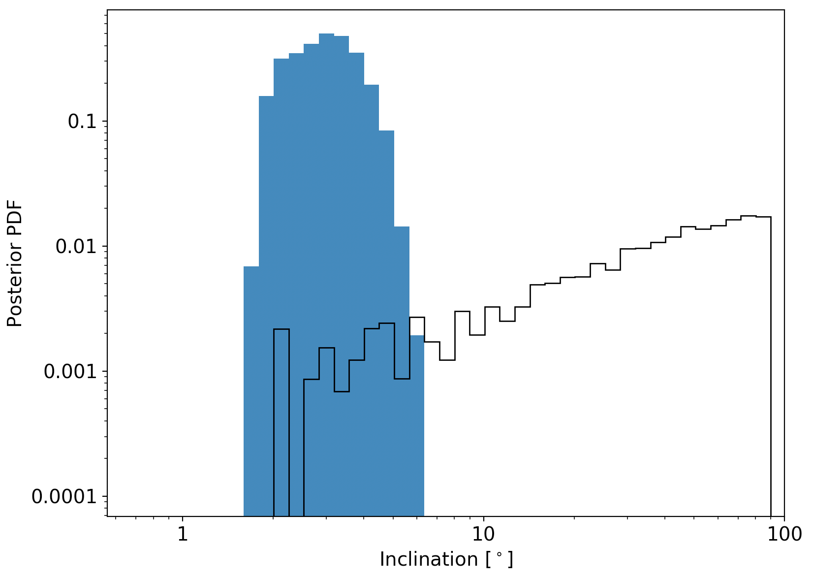
Figure 9: Same as Fig. 7, illustrating situation #1, with the secondary dataset source companion HD 16760 b ($P$=465 days, $a_{\star}\sin i$=0.25 mas and $\varepsilon_{\text{DR1}}$=3 mas).

5.2.2 SItuation #2: upper-limit constraint on companion mass

The orbit inclination of 18 companions from 17 different systems in the detection sample cannot be fully determined using GASTON. For those orbits, the simulated astrometric excess noise is often compatible with $\varepsilon_{\text{DR1}}$ from $I_{c}$=90^∘ down to $\sim$0^∘. Accounting for the $\sin I_{c}$ prior probability distribution on the inclination, the MCMC leads to a posterior distribution for which the 3-$\sigma$ upper-bound on inclination is located beyond 89.5^∘. More accurately, the posterior distribution on their orbit inclination and mass are mainly fixed by the $\sin I_{c}$ prior on inclination.

As presented in Table 8, all these candidates are possible planets at the 1-$\sigma$ limit. Excluding the transiting planets which are known to be bona-fide planets on edge-on orbits, only two of them have a true mass below, but close to, the Deuterium burning limit of 13.5 M${}_{\text{J}}$. They are HD 164595 b and HD 185269 b with a mass smaller than respectively 12.9 and 12.6 M${}_{\text{J}}$ at 3-$\sigma$. Those two seem thus likely to be actual planets with a mass in the Neptunian (0.06 M${}_{\text{J}}$ for HD 164595 b) and Jupiterian (1.12 M${}_{\text{J}}$ for HD 185269 b) domain.

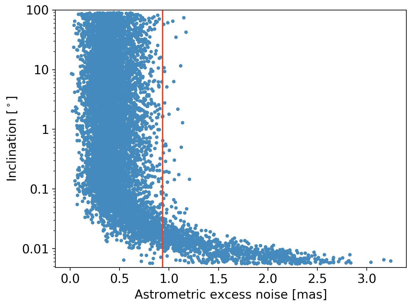
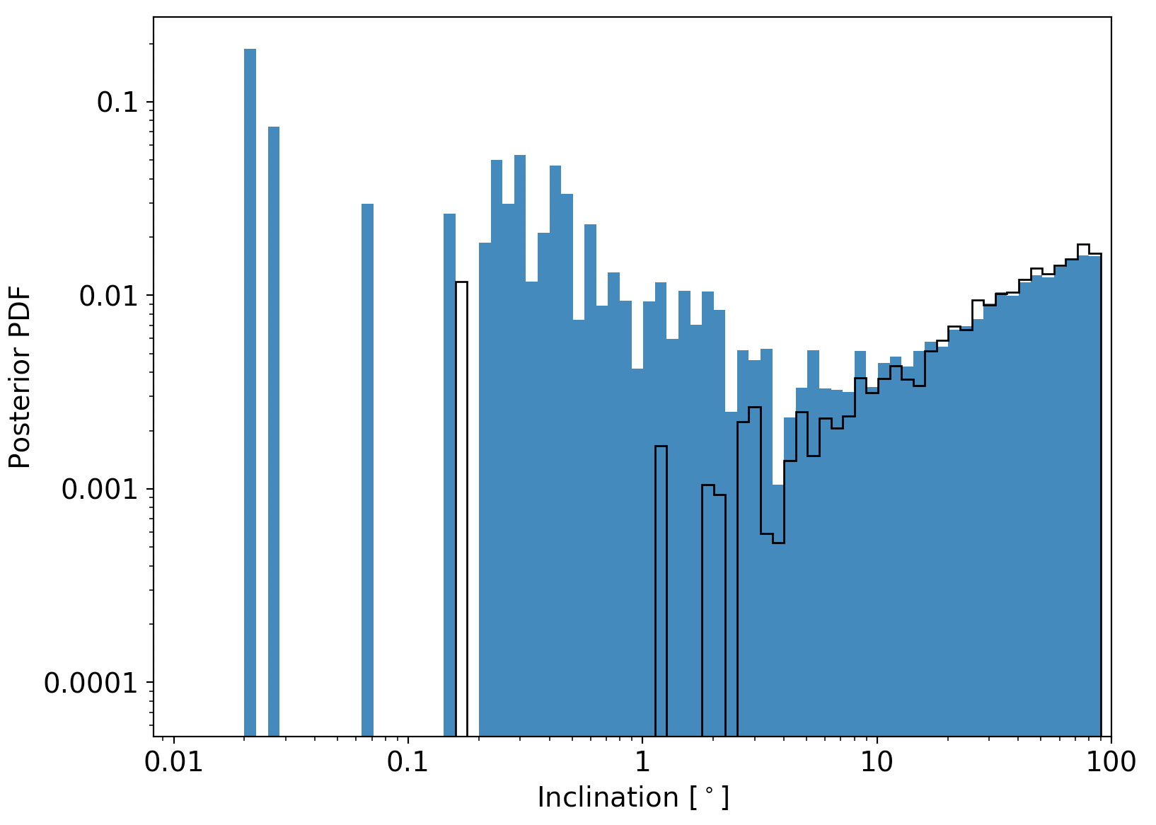
Figure 10: Illustration of situation #2 with HD 164595 b, $P$=40 days, $a_{\star}\sin i$=0.0004 mas and $\varepsilon_{\text{DR1}}$=0.93 mas. Many simulations from $I_{c}$=0.1^∘ up to 90^∘ are compatible with $\varepsilon_{\text{DR1}}$. This reflects in the comparison of the $I_{c}$ posterior to the $\sin I_{c}$ prior PDFs shown in black.

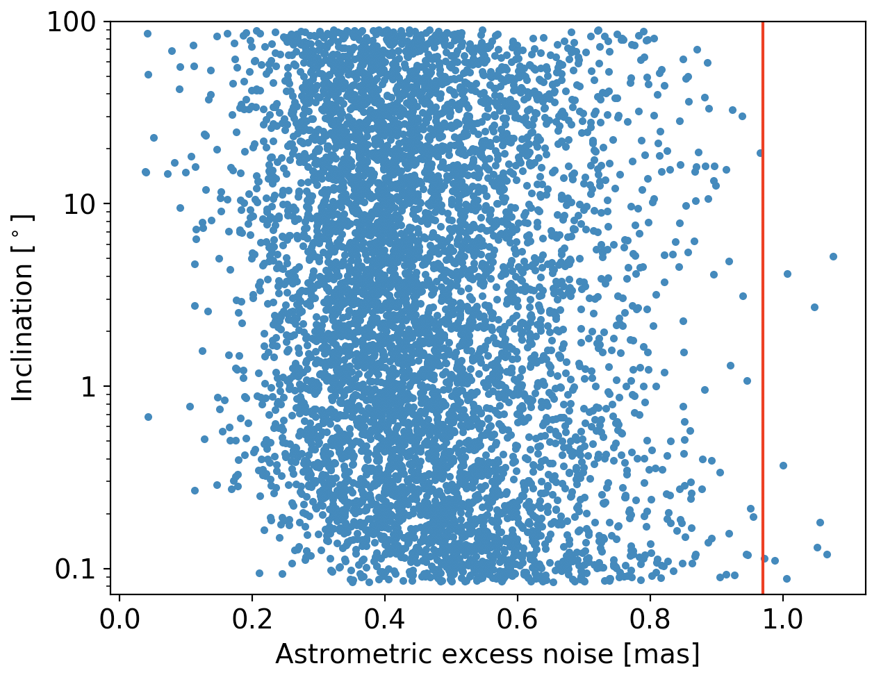
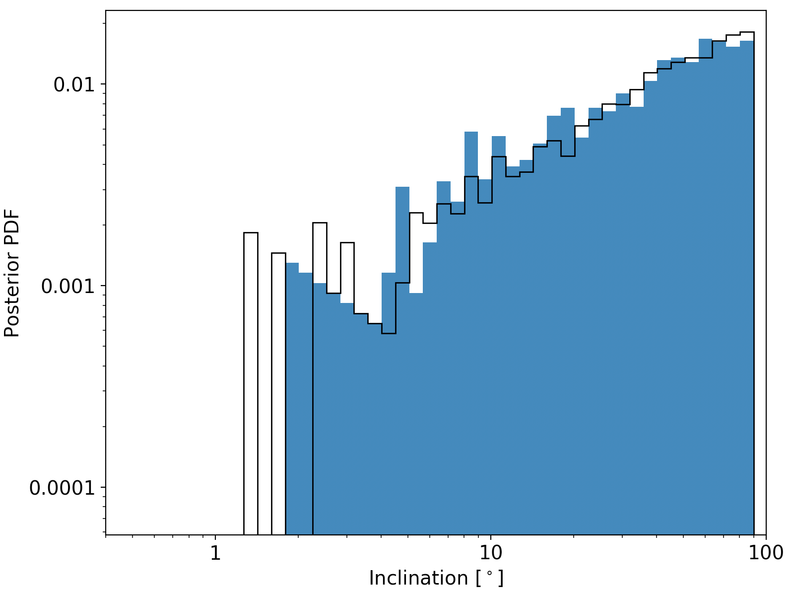
Figure 11: Same plot as Fig. 10, illustrating situation #2, with HD 185269 b ($P$=6.8 days, $a_{\star}\sin i$=0.001 mas and $\varepsilon_{\text{DR1}}$=0.97 mas). Many simulations from about $I_{c}$=0.1^∘ up to 90^∘ are compatible with $\varepsilon_{\text{DR1}}$ thanks to noise. Smaller inclinations are rejected due to too large mass and luminosity for the companion. The posterior distribution in the bottom panel is fully compatible with the prior $\sin I_{c}$ PDF.

We note however that HD 164595 is a duplicate source in the Gaia DR1. Its astrometric excess noise, and thus the mass of HD 164595 b, might be underestimated (see the discussion on this specific issue in Section 3.1). Moreover, for both companions, the simulated astrometric excess noise is indeed compatible with $\varepsilon_{\text{DR1}}$ on a large range of inclinations (Figs. 10 and 11). The posterior distributions of $I_{c}$ and $M_{c}$ are essentially due to the prior distribution on $I_{c}$. If the actual prior distribution of $I_{c}$ is biased towards $0^{\circ}$ (see the related discussion in Section 6.2), it cannot be excluded that the masses of HD 164595 b and HD 185269 b are actually larger than 13.5 M${}_{\text{J}}$.

Seven companions are transiting planets. They are HAT-P-21 b, WASP-11 b, WASP-17 b, WASP-131 b, WASP-157 b and K2-34 b in the primary dataset, and K2-110 b in the secondary dataset. Gaia DR1 measurements all are compatible with the edge-on configurations. The MCMC acceptance rates are smaller than 0.01 with a star semi-major axis smaller than 1 $\mu$as. It can be excluded that Gaia will truly detect the reflex motion of these stars due to their transiting exoplanets.

Two exoplanet candidates are part of a common multiple system, HD 154857 b and c. The Gaia observations are compatible with an edge-on inclination and masses of 2.2 and 2.5 M${}_{\text{J}}$. At 1-$\sigma$ the posterior distributions, conformally to the $\sin I_{c}$ prior distribution on $I_{c}$, allow inclinations as low as 20^∘ with masses as large as 6 M${}_{\text{J}}$, but at 3-$\sigma$ their mass could be as large as 135 and 175 M${}_{\text{J}}$. Both companions are thus possible Jupiter-mass planets with masses within 2-6 M${}_{\text{J}}$, but their true nature could not be confirmed.

5.2.3 Situation #3: incompatible RV orbit and Gaia astrometry

The GASTON results for the two companions within this situation are presented in Table 7. They are WASP-43 b and WASP-156 b, both transiting planets on compact orbit ($P$=0.8 days and 3.8 days). In these two systems, none of the published companions are adequate for explaining Gaia’s observations. The maximum astrometric excess noise that could be simulated from RV orbital parameters were respectively 1.25 and 1.32 mas, well below the $\varepsilon_{\text{DR1}}$ of these two sources, respectively 2 mas and 1.5 mas. These two sources from the secondary dataset are not mentioned as duplicated sources in the DR1 database.

There are three possible scenarios for explaining this RV-Gaia discrepancy:

• The value of the astrometric excess noise could depend on the presence of fortuitous outliers. With a number of astrometric measurements $\sim$50 per source, outliers of several mas could slightly inflate $\varepsilon_{\text{DR1}}$ with a discrepancy of a few 0.1 mas. Outliers larger than $4.8$$\times$$\varepsilon_{\text{DR1}}$$\sim$$10$ mas (see note 7 in Lindegren et al. 2016) are flagged as ”bad” during the AGIS reduction and discarded. Therefore, the discrepancy observed in Table 7 for the 2 companions between the highest $\varepsilon_{\text{simu}}$ and $\varepsilon_{\text{DR1}}$ of 0.2-0.7 mas could be explained by numerous or large outliers. We cannot exclude this possibility without analysing the time series, which will not be available until the final Gaia release in a few years.

• Instrumental and modeling noises larger than those adopted in Section 3.4 could allow reaching the astrometric excess noise. Indeed, for the astrometric data of secondary dataset targets the parallax and proper motion fit is not of good quality, and could individually reach high astrometric excess noise, as indicated by the 90th-percentile $\varepsilon_{\text{DR1}}$=2.3 mas measured by Lindegren et al. (2016) in the full secondary dataset. Although plausible, as already discussed in Section 3.4, the good match between the distribution of simulated and observed $\varepsilon_{\text{DR1}}$ implies that the instrumental and modeling noise cannot be much larger than the adopted range of 0.4-0.9 mas in the present sample.

• A hidden outer companion to the system, unseen in the RV variations, could be responsible for the astrometric signal. This issue is discussed in Section 6.4.

Although the presence of outliers cannot be excluded, this RV-Gaia discrepancy motivates the search for supplementary yet hidden companions in these systems.

Table 7: The two exoplanets WASP-43 b and WASP-156 b, which RV orbit is incompatible with Gaia astrometric excess noise. The maximum astrometric excess noise that we were able to simulate for these secondary dataset sources is given as $\varepsilon_{\text{simu,max}}$.

Parameter	Unit	WASP-43 b	WASP-156 b
Period	(day)	0.813	3.836
$m\sin i$	(M${}_{\text{J}}$)	1.761	0.131
$a\sin i$	(mas)	0.00047	0.000055
$\varepsilon_{\text{DR1}}$	(mas)	1.96	1.49
$\varepsilon_{\text{simu,max}}$	(mas)	1.25	1.32

5.3 Non-detection sample: 27 confirmed planets

For a given RV orbit with given $m\sin i$ of the companion, an increasing true mass and thus decreasing orbital inclination imply increasing astrometric motion of the star. The non-detection of an astrometric excess noise larger than the defined threshold thus allow deriving an upper-limit on the true mass of the companion and a lower-limit on its orbital inclination with GASTON.

Among the 227 non-transiting companions of the non-detection sample, we constrained true masses lower than 13.5 M${}_{\text{J}}$ within 3-$\sigma$ confidence interval for a total of 27 companions. They are summarized in Table 9. Nine planets have a true mass lower than 5 M${}_{\text{J}}$, and 19 have a true mass lower than 10 M${}_{\text{J}}$.

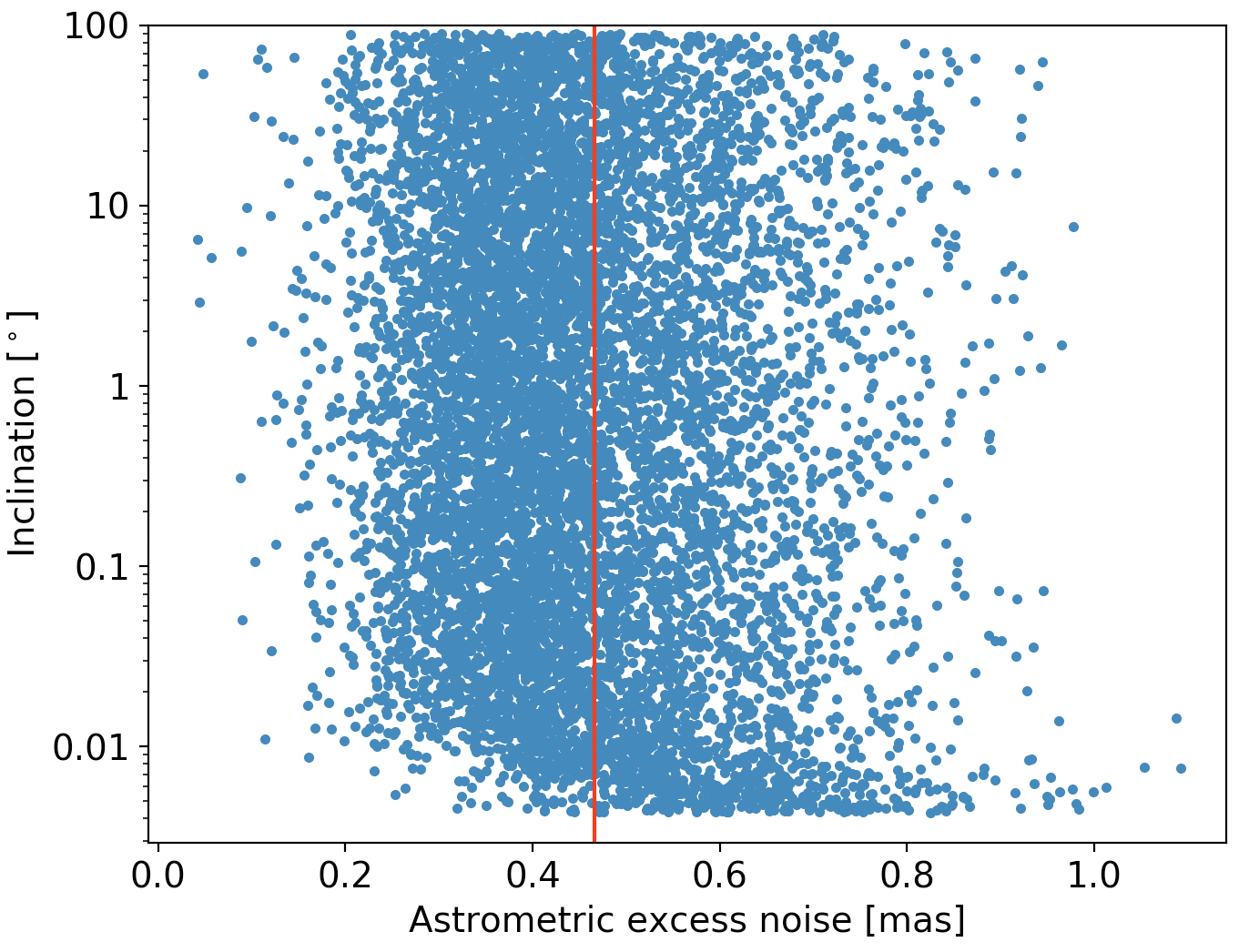
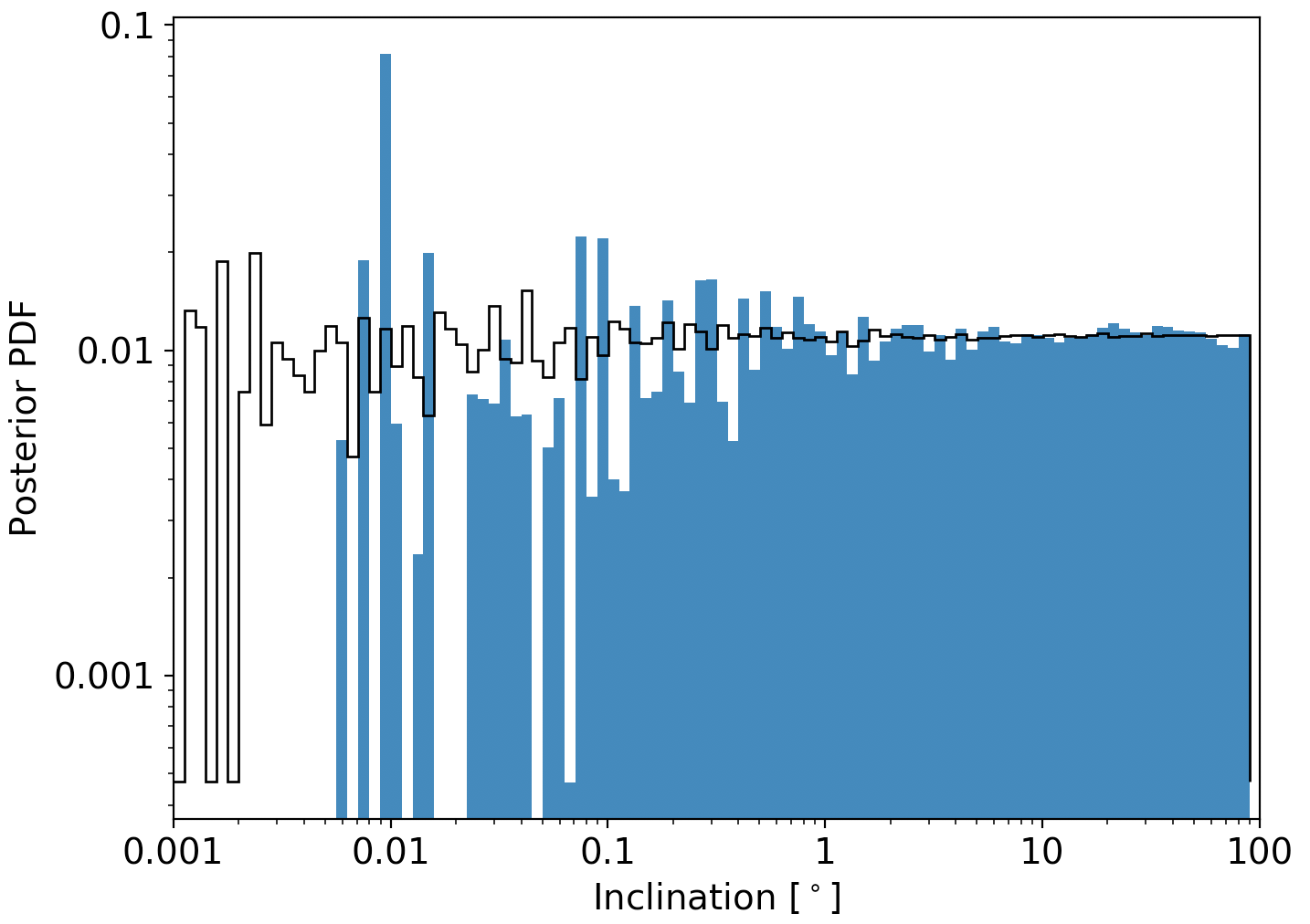
Figure 12: An example of a confirmed planet from the non-detection sample with HD 10180 c ($P$=5.8 days, $m\sin i$=0.041 M${}_{\text{J}}$, $\varepsilon_{\text{DR1}}$=0.47 mas). Top & bottom panels: same as Fig. 7, only the black line in the bottom panel now represents inclinations drawn from a uniform distribution.

We confirm that 6 multiple system contains several true planets. They are HD 10180, HD 176986, HD 181433, HD 215152, HD 7924, and HD 40307. In the 6-planets system, HD 10180, we can confirm that the a priori less massive companions c ($P$=5.8 days, $m\sin i$=0.041 M${}_{\text{J}}$), d ($P$=16.4 days, $m\sin i$=0.037 M${}_{\text{J}}$), and g ($P$=602 days, $m\sin i$=0.067 M${}_{\text{J}}$) are planets with a mass strictly lower than 12 M${}_{\text{J}}$ at 3-$\sigma$. Fig. 12 shows the $\varepsilon_{\text{simu}}$–$I_{c}$ relationship and $I_{c}$ posterior distribution for HD 10180 c. A study of the effect of mutual inclinations on the stability of this system led to constrain the masses of the planets within a factor of 3, with $I_{c}$$>$$10^{\circ}$ for all planets (Lovis et al. 2010). While our result is not as much as restrictive, it excludes a full face-on inclination with $I_{c}$$>$$0.2^{\circ}$ at 3-$\sigma$ and confirms planetary mass for planets c, d, and g.

Table 8: GASTON results for the 29 companions in the detection sample, and divided into the two different situations mentioned in the text.

Planet name	Period	$m\sin i$	$a\sin i$	$\epsilon$	$a_{\text{phot}}$		$I_{c}$		$M_{\text{c,true}}$		$\Delta V$		MCMC
	(days)	(M${}_{\text{J}}$)	(mas)	(mas)	(mas)	(mas)	(∘)		(M${}_{\text{J}}$)				Acceptance
					1-$\sigma$	3-$\sigma$	1-$\sigma$	3-$\sigma$	1-$\sigma$	3-$\sigma$	1-$\sigma$	3-$\sigma$	rate
First situation: strong constraint on inclination and mass
Primary dataset:
30 Ari B b	335.1	9.878	0.1728	1.777	$2.391_{-0.444}^{+0.592}$	$(1.347,5.948)$	$4.181_{-0.931}^{+1.031}$	$(1.643,7.584)$	$147.4_{-29.5}^{+41.3}$	$(78.92,412.5)$	$11.14_{-1.47}^{+1.05}$	$(6.888,16.46)$	0.2321
HD 114762 b	83.92	11.64	0.1161	1.088	$1.339_{-0.353}^{+0.302}$	$(0.4206,2.597)$	$4.940_{-0.942}^{+1.773}$	$(2.517,15.76)$	$147.0_{-42.0}^{+39.3}$	$(41.93,323.9)$	$9.350_{-1.413}^{+1.614}$	$(5.704,22.37)$	0.1758
HD 141937 b	653.2	9.475	0.3955	0.9337	$1.126_{-0.401}^{+0.272}$	$(0.3798,2.047)$	$20.52_{-4.16}^{+12.47}$	$(11.01,88.85)$	$27.42_{-9.86}^{+6.78}$	$(9.061,50.94)$	$24.38_{-0.61}^{+1.29}$	$(22.82,29.59)$	0.1340
HD 148427 b	331.5	1.144	0.01182	1.092	$1.329_{-0.310}^{+0.332}$	$(0.4964,2.936)$	$0.5120_{-0.1082}^{+0.1635}$	$(0.2314,1.413)$	$136.5_{-33.7}^{+37.2}$	$(47.74,336.0)$	$12.34_{-1.32}^{+1.26}$	$(8.368,24.50)$	0.1866
HD 5388 b	777.0	1.965	0.05154	1.365	$2.182_{-0.255}^{+0.330}$	$(1.519,3.923)$	$1.356_{-0.191}^{+0.195}$	$(0.7610,2.050)$	$87.02_{-10.80}^{+13.99}$	$(60.02,163.3)$	$14.95_{-1.82}^{+4.58}$	$(10.81,23.13)$	0.2394
HD 6718 b	2496	1.559	0.1087	1.121	$4.201_{-0.881}^{+1.092}$	$(1.982,9.951)$	$1.488_{-0.310}^{+0.410}$	$(0.6181,3.688)$	$62.79_{-13.80}^{+16.98}$	$(27.74,159.7)$	$21.22_{-5.60}^{+1.20}$	$(9.348,24.13)$	0.2073
HD 96127 b	647.3	4.007	0.01116	1.124	$0.6640_{-0.6457}^{+0.7888}$	$(0.0009983,2.231)$	$1.364_{-0.763}^{+38.527}$	$(0.4084,89.54)$	$190.2_{-184.0}^{+284.1}$	$(3.359,679.2)$	$8.008_{-3.522}^{+16.829}$	$(2.526,26.81)$	0.05775
HIP 65891 b	1084	6.001	0.04197	1.146	$2.040_{-0.341}^{+0.409}$	$(1.103,4.026)$	$1.184_{-0.207}^{+0.256}$	$(0.5929,2.161)$	$312.3_{-57.4}^{+74.2}$	$(168.4,713.7)$	$10.85_{-0.63}^{+0.65}$	$(7.196,13.52)$	0.2000
Secondary dataset:
HD 16760 b	465.1	13.29	0.2531	2.990	$4.467_{-0.758}^{+1.053}$	$(2.758,7.364)$	$3.164_{-0.762}^{+0.810}$	$(1.796,5.549)$	$291.9_{-69.4}^{+120.7}$	$(151.8,580.9)$	$5.154_{-1.124}^{+0.926}$	$(2.517,8.215)$	0.2521
Second situation: lower and upper limits on inclination and mass
Primary dataset:
HAT-P-21 b	4.124	4.073	0.0007560	0.9171	$<$0.0014260	$<$0.01209	$>$32.88	$>$4.067	$<$7.542	$<$57.72	$>$14.79	$>$13.58	0.009911
HD 132563 B b	1544	1.492	0.03442	0.8536	$<$0.07070	$<$2.621	$>$29.25	$>$0.8231	$<$3.050	$<$111.1	$>$25.10	$>$11.03	0.01422
HD 154857 b	408.6	2.248	0.02508	0.9309	$<$0.05492	$<$1.499	$>$27.03	$>$1.014	$<$4.918	$<$134.9	$>$24.71	$>$13.10	0.009493
HD 154857 c	3452	2.579	0.1193	0.9309	$<$0.2729	$<$8.817	$>$25.98	$>$0.9194	$<$5.905	$<$175.3	$>$27.78	$>$10.97	0.009493
HD 164595 b	40.00	0.05078	0.0003920	0.9341	$<$0.0008560	$<$0.1093	$>$27.67	$>$0.2476	$<$0.11103	$<$12.86	$>$24.46	$>$22.70	0.01065
HD 177830 b	410.1	1.320	0.01953	0.8723	$<$0.04035	$<$1.278	$>$28.82	$>$1.019	$<$2.738	$<$78.92	$>$24.47	$>$13.43	0.01443
HD 185269 b	6.838	0.9542	0.001040	0.9694	$<$0.002002	$<$0.01755	$>$31.18	$>$4.624	$<$1.820	$<$12.34	$>$19.00	$>$18.87	0.005830
HD 190228 b	1136	5.942	0.1278	0.8628	$<$0.5136	$<$2.375	$>$14.25	$>$3.188	$<$24.418	$<$111.4	$>$27.35	$>$14.34	0.02329
HD 197037 b	1036	0.8073	0.04322	0.9947	$<$0.12112	$<$3.087	$>$21.09	$>$0.8682	$<$2.2696	$<$55.87	$>$27.13	$>$22.28	0.008977
HD 4203 b	431.9	2.082	0.02595	0.8539	$<$0.05646	$<$1.390	$>$27.46	$>$1.116	$<$4.533	$<$110.2	$>$24.02	$>$11.82	0.02863
HD 7449 b	1275	1.313	0.07578	0.9430	$<$0.16248	$<$6.525	$>$30.30	$>$0.8955	$<$2.845	$<$104.2	$>$27.17	$>$11.48	0.01279
HD 95127 b	482.0	5.036	0.006734	1.220	$<$0.017628	$<$0.3977	$>$26.57	$>$2.027	$<$11.863	$<$170.2	$>$23.04	$>$6.939	0.001910
K2-34 b	2.996	1.683	0.0001870	0.9982	$<$0.0004070	$<$0.002572	$>$28.51	$>$3.946	$<$3.525	$<$23.91	$>$13.63	$>$12.40	0.002133
WASP-11 b	3.722	0.5398	0.0002100	1.064	$<$0.0004260	$<$0.004463	$>$29.21	$>$3.117	$<$1.1059	$<$9.719	$>$15.62	$>$15.27	0.003389
WASP-131 b	5.322	0.2724	0.00006800	0.9476	$<$0.00014300	$<$0.001557	$>$28.30	$>$4.120	$<$0.5756	$<$3.710	$>$15.31	$>$14.62	0.01006
WASP-157 b	3.952	0.5592	0.00008400	0.8699	$<$0.0001670	$<$0.001673	$>$30.85	$>$3.765	$<$1.1127	$<$8.444	$>$14.31	$>$13.06	0.01517
WASP-17 b	3.735	0.5077	0.00005200	0.8509	$<$0.00010000	$<$0.0007792	$>$32.14	$>$5.985	$<$0.9619	$<$4.768	$>$13.48	$>$12.70	0.006831
Secondary dataset:
K2-110 b	13.86	0.05293	0.00006000	1.278	$<$0.00069800	$<$0.01073	$>$4.96	$>$0.3551	$<$0.62324	$<$6.732	$>$18.03	$>$17.49	0.0007182

Table 9: GASTON results for 27 exoplanet candidates from the non-detection sample. Their 3-$\sigma$ upper-limit on mass is smaller than 13.5 M${}_{\text{J}}$ and the convergence criterion $N_{\text{step}}/\text{max}(\tau_{\lambda}$$\geq$$50$. We expand this table in the Appendix, Table LABEL:tab:results_nondet_comp, with the rest of the exoplanet candidates among the non-detection sample and for which $M_{\text{max,}3\sigma}$¿13.5 M${}_{\text{J}}$.

Planet name	Period	$m\sin i$	$a\sin i$	$\epsilon$	$a_{\text{phot}}$	$I_{c}$	$M_{\text{c,true}}$	$\Delta V$	MCMC
	(days)	(M${}_{\text{J}}$)	(mas)	(mas)	(mas)	(∘)	(M${}_{\text{J}}$)	Acceptance
					3-$\sigma$	3-$\sigma$	3-$\sigma$	3-$\sigma$	rate
3-$\sigma$ limits, with $M_{\text{c,true}}$$<$$13.5$ M${}_{\text{J}}$ at 3-$\sigma$
Primary dataset: 24 confirmed exoplanets
BD -06 1339 b	3.873	0.02680	0.00007800	0.5190	$<$0.03085	$>$0.3243	$<$4.792	$>$19.77	0.1357
BD -08 2823 b	5.600	0.04594	0.00008000	0.4011	$<$0.02921	$>$0.2746	$<$9.277	$>$18.80	0.1914
HD 10180 c	5.760	0.04151	0.00006200	0.4662	$<$0.01925	$>$0.2841	$<$8.626	$>$19.26	0.1585
HD 10180 d	16.36	0.03766	0.0001120	0.4662	$<$0.06159	$>$0.2005	$<$10.37	$>$20.77	0.1592
HD 10180 g	602.0	0.06738	0.002221	0.4662	$<$0.4390	$>$0.3663	$<$10.62	$>$25.92	0.1496
HD 125595 b	9.674	0.04168	0.0001510	0.4106	$<$0.08048	$>$0.2243	$<$11.11	$>$20.48	0.2058
HD 154345 b	3342	0.9569	0.2360	0.3491	$<$3.454	$>$4.652	$<$11.94	$>$26.02	0.1737
HD 175607 b	29.03	0.02626	0.0001440	0.4171	$<$0.07016	$>$0.1865	$<$7.728	$>$21.26	0.1692
HD 176986 b	6.490	0.02002	0.00005500	0.2559	$<$0.02388	$>$0.2581	$<$4.681	$>$19.98	0.1911
HD 176986 c	16.82	0.02814	0.0001450	0.2559	$<$0.05738	$>$0.2419	$<$6.601	$>$21.35	0.1939
HD 179079 b	14.48	0.08378	0.0001240	0.3794	$<$0.03729	$>$0.3766	$<$13.20	$>$19.21	0.1853
HD 181433 b	9.374	0.02373	0.00008600	0.2972	$<$0.04037	$>$0.2542	$<$5.376	$>$20.49	0.1210
HD 181433 c	962.0	0.6404	0.05114	0.2972	$<$0.6246	$>$5.196	$<$6.944	$>$27.15	0.1185
HD 181433 d	2172	0.5355	0.07359	0.2972	$<$1.747	$>$2.665	$<$11.28	$>$25.41	0.1186
HD 215152 b	5.760	0.005720	0.00001900	0.3057	$<$0.009679	$>$0.1871	$<$1.779	$>$20.36	0.1786
HD 215152 c	7.282	0.005408	0.00002100	0.3057	$<$0.01000	$>$0.2035	$<$1.475	$>$20.70	0.1799
HD 215152 d	10.86	0.008816	0.00004400	0.3057	$<$0.02144	$>$0.1998	$<$2.424	$>$21.27	0.1783
HD 215152 e	25.20	0.009052	0.00008000	0.3057	$<$0.04964	$>$0.1869	$<$3.069	$>$22.48	0.1794
HD 215497 b	3.934	0.02085	0.00002600	0.4831	$<$0.01194	$>$0.2301	$<$4.999	$>$18.50	0.1164
HD 7199 b	615.0	0.2950	0.01192	0.3742	$<$0.5161	$>$1.496	$<$11.45	$>$25.73	0.1817
HD 7924 b	5.398	0.02737	0.0001050	0.5727	$<$0.04275	$>$0.2472	$<$6.476	$>$20.81	0.1021
HD 7924 c	15.30	0.02484	0.0001900	0.5727	$<$0.08133	$>$0.2575	$<$5.546	$>$22.31	0.1015
HD 7924 d	24.45	0.02038	0.0002130	0.5727	$<$0.1022	$>$0.2188	$<$4.934	$>$22.99	0.1091
HIP 57274 b	8.135	0.03657	0.0001300	0.4507	$<$0.06026	$>$0.1980	$<$10.57	$>$20.32	0.1738
Secondary dataset: 3 confirmed exoplanets
HD 40307 b	4.311	0.01291	0.00006000	0.3337	$<$0.03068	$>$0.2022	$<$3.741	$>$20.72	0.1891
HD 40307 c	9.620	0.02115	0.0001690	0.3337	$<$0.07895	$>$0.2109	$<$5.879	$>$21.69	0.1899
HD 40307 d	20.46	0.02808	0.0003710	0.3337	$<$0.1125	$>$0.2855	$<$5.586	$>$22.81	0.1927

Among the 200 other candidate planets, as summarized in Table LABEL:tab:results_nondet_comp, 103 companions can be confirmed substellar but may be as massive as brown dwarfs with a mass strictly smaller than 85 M${}_{\text{J}}$ at 3-$\sigma$, and 59 others have a mass upper-limit within the M-dwarf domain. For the remaining 48 companions, GASTON could not converge within the 50,000 steps, with an autocorrelation length larger than 1000. At the end of the GASTON run, the posterior distributions for all of them led to an upper-limit on the mass larger than 13.5 M${}_{\text{J}}$. This non-convergence is due to a large astrometric excess noise but smaller than the detection limit. Simulations are less often compatible with $\varepsilon_{\text{DR1}}$, GASTON thus needs more time to converge. Their nature is undetermined between planet, BD and M-dwarf. We do not publish GASTON results for those 48 candidates.

While most of companions with a mass possibly greater than 13.5 M${}_{\text{J}}$ have large orbital periods, 30 of them have an orbital period smaller than 100 days. Those are possible BD located within the driest region of the brown-dwarfs detection desert (Kiefer et al. 2019). They are particularly interesting objects that need to be further characterized in order to better constrain the shores of the BD mass-period phase space.

6 Discussion

6.1 A revised mass for 9 companions

Figure 13 summarizes the corrected mass derived with GASTON compared to the initial $m\sin i$ as given in the Exoplanets.org database. The firm measurements for the 9 companions identified in Section 5.2.1 lead to true masses significantly different from the $m\sin i$ with an non edge-on inclination. Their revised mass is generally comprised between 10 and 500 M${}_{\text{J}}$, as are the 3-$\sigma$ upper-limits reported for companions from situation #2 and in the non-detection sample.

This shows that Gaia will be best at detecting astrometric motions due to companions beyond $\sim$10 M${}_{\text{J}}$. But with improved precision in the future releases and the use of time series, it will certainly allow the detection of Jupiter mass planets.

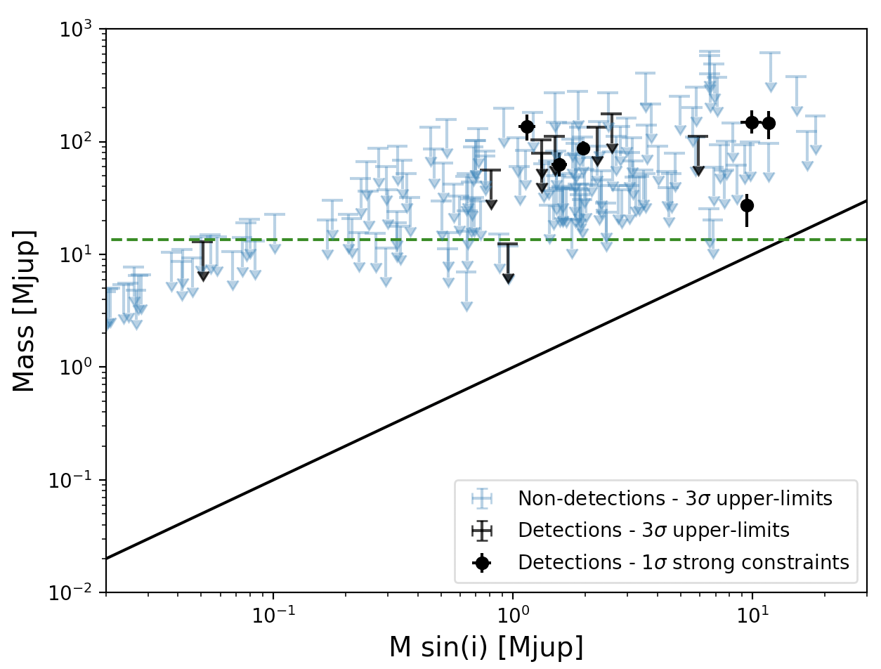
Figure 13: Masses and upper-limits derived with GASTON for 191 companions directly compared to the $m\sin i$ derived from RVs. The black solid line represents the relation $M_{\text{true}}$=$m\sin i$ obtained for an edge-on inclination of the orbits. The green dashed line marks the 13.5-M${}_{\text{J}}$ deuterium-burning limit.

6.2 Small inclinations $<$4^∘

To our knowledge, no exoplanet RV candidate from the exoplanets.org database were yet found with an inclination strictly lower than 4^∘. The exoplanet with the smallest known orbital inclination is Kepler-419 c with $I_{c}$=2.5$\pm$3^∘, thanks to transit timing variations (Dawson et al. 2014). In Table 8, among the 9 non-transiting systems with a firmly detected inclination, and accounting for their 3-$\sigma$ bounds, we find zero companion with $I_{c}$ strictly smaller than $1^{\circ}$, one companion, HD 148427 b, with $I_{c}$ strictly smaller than $2^{\circ}$, and four others with $I_{c}$ strictly smaller than 4^∘. Many other companions from the detection and non-detection samples could have such small inclinations, but also posibly larger than 1, 2 or $4^{\circ}$. Assuming isotropy of orbits within the $\sim$600 known non-transiting RV exoplanets in the exoplanets.org database leads to less than 0.4 orbits with $I_{c}$$\leq$$2^{\circ}$ and less than 1.5 orbits with $I_{c}$$\leq$$4^{\circ}$. Finding more than 1 system with an orbit less inclined than 2^∘ and more than 4 with $I_{c}$$<$$4^{\circ}$ suggests that the distribution of inclinations within exoplanet candidates deviates from a uniform distribution at least below $4^{\circ}$. This questions the isotropy of orbits within the population of discovered RV exoplanets advocated in e.g. Zucker & Mazeh (2001b), Jorissen et al. (2001) and Tabachnik & Tremaine (2002). It was indeed already noticed in Halbwachs et al. (2000) and Han et al. (2001) that RV-planet systems are possibly biased towards small $\sin i$.

The uniform distribution of inclinations certainly applies on a larger sample of systems than just RV exoplanets hosting systems. SB1 binary companions ($M_{c}$$<$$0.6$ $M_{\star}$) on orbits with inclinations $<$2^∘ would most likely fall within exoplanetary domain. A $\sin i$$<$$0.035$ would indeed lead to $M\sin i$$<$$20(M_{\star}/M_{\odot})$ M${}_{\text{J}}$. Several thousands of binary systems and stars were, and are still being, followed-up for RV variations for many years. About 1300 SB1 binaries are collected in the SB9 database (Pourbaix et al. 2004) and about 600 RV systems (excluding all transiting planets that are biased to 90^∘). Probably twice as many are still being followed-up, neither characterized nor published yet. We thus estimate the full population of RV-monitored systems possibly, or actually, harboring planets or hidden binary component to reach at least 4000 individuals, among which FGK stars are the dominating class of stellar primaries. Assuming isotropy of orbits in this larger sample, we expect to observe at least $\sim$0.6 systems with an inclination $\leq$1^∘, $\sim$2.4 systems with $I_{c}$$\leq$$2^{\circ}$ and $\sim$9.7 systems with $I_{c}$$\leq$$4^{\circ}$. This is in better agreement with our findings, validating the GASTON determination of orbital inclinations for RV companions with the Gaia DR1.

6.3 Systems with edge-on transiting orbits

In Section 3.3, we found 9 over 246 systems (i.e. 3.7% of them) with transiting-only planets to have an astrometric excess noise larger than the defined thresholds for a significant astrometric motion. Six of them are systems around sources from the primary dataset. Given their edge-on orbit, with an expected astrometric semi-major axis of the photocenter on the order of a few $\mu$as, it is technically impossible to detect their host star’s reflex motion with Gaia. But the measurement of $\varepsilon_{\text{DR1}}$ beyond the threshold suggests on the contrary that a significant astrometric motion was actually detected.

Running GASTON brings a solution to this inconsistency. For 7 among 9 companions, an edge-on astrometric orbit is compatible with the value of $\varepsilon_{\text{DR1}}$, because instrumental and measurement noises can pile up to produce an astrometric excess noise above the threshold. However, this compatibility is far from being frequent in the MCMC runs, as shown by the low acceptance ratio in both cases ($<$1.5%; see Table 8). Could it be that $\varepsilon_{\text{DR1}}$ is actually not due to instrumental and measurement noise for some of them, and leads to truly incompatible astrometric motion?

To test this possibility, we simulated many Gaia observations of non-accelerating stars, with $N_{\text{FoV}}$ and $N_{\text{AL}}$ drawn from the sample of 133 systems with transiting-only planets from the primary dataset, and the 113 systems with transiting-only planets from the secondary dataset. In the primary dataset, this results into 6 over 133 astrometric excess noise values beyond 0.85 mas, produced only from noise, with a probability of 0.0014, i.e. below 3 $\sigma$. Producing 5 over 133 astrometric excess noise values beyond 0.85 mas has a probability of 0.0072, i.e. above 3 $\sigma$. In the secondary dataset, the probability to produce 2 or 3 over 113 astrometric excess noise values beyond 1.2 mas is smaller than 0.0001, while producing 1 over 113 is significantly more likely with a probability of 1.2%.

Thus for at least one system from the primary dataset, possibly K2-34 with the lowest MCMC acceptance rate of 0.002, Gaia detected a signal that cannot be fully explained by the combination of the published orbit and noise. This could be the sign of an unseen and unknown outer companion in the system of K2-34, or a measurable effect of outliers (see the discussion in Section 5.2.3 for WASP-43 b and WASP-156 b).

In the secondary dataset, no more than one system among 113 could be simulated with an astrometric excess noise as large as 1.2 mas. Consistently, we recall obtaining a marginal compatibility of GASTON simulations with $\varepsilon_{\text{DR1}}$ only for K2-110 b (Section 5.2.2), and no compatibility at all for two other planets, WASP-43 b and WASP-156 b (Section 5.2.3). We conclude that noise is the likely explanation for the astrometric excess noise of K2-110 b. As already discussed in Section 5.2.3, the most reasonable explanations for the large inconsistent $\varepsilon_{\text{DR1}}$ of WASP-43 and WASP-156 are either unmodeled outliers, or the presence of an outer companion in both systems.

We conclude that follow-ups of K2-34, WASP-43 and WASP-156 should be conducted to search for outer companions in these edge-on systems.

6.4 Outer companions

In the cases with the lowest acceptance rates in Table 8, it could be that the astrometric signal is better explained by the influence of another outer companion to the system, especially if as for HD 4203, a long-period RV-drift is detected (Kane et al. 2014). With a minimum mass of at least 2 M${}_{\text{J}}$, this outer companion with an orbital period of several thousands of days (tens of year) might also be at the origin of the astrometric signal.

As mentioned in Section 6.3, the astrometric excess noise of few compact edge-on systems (K2-34, WASP-43 and WASP-156) is difficult, and even impossible, to produce with our simulations. Thus, while outliers could explain the discrepancy of the RV orbit and Gaia astrometry, a more simple explanation could be the presence of an outer companion. There are no clues of long RV drifts in neither of these systems, but this does not invalidate the hypothesis of an outer companion because the orbital inclination can be adjusted to make the RV signal vanish.

More generally, for any system in situation #1 leading to a mass measurement of an RV companion, the presence of an unknown outer companion cannot be totally excluded. Nevertheless, as far as we know these systems, the solution with the less complexity is preferred, i.e. the known RV-orbit with a realistic inclination is responsible for the Gaia measurement of the star motion. Fine-tuned mass, semi-major axis and inclination of an unknown unseen companion’s orbit would be necessary to explain the astrometric excess noise, while using the existing known companion on a known orbit only require to fit a single parameter, the inclination.

We have shown in Section 3.3 that the astrometric excess noise is not correlated to the presence of an RV-drift, and thus to the presence of an outer companion on an undetermined orbit. Thus, a large astrometric excess noise does not imply the presence of an outer companion and conversely the presence of an outer companion does not imply a large astrometric excess noise. It was already shown for HD 114762 b (Kiefer 2019) that the binary companion HD 114762 B, a low-mass star at several hundred au separation and with orbital period much larger than the Gaia DR1 campaign duration of 416 days, only has a minor impact on the motion of HD 114762 A. It was better explained by a small orbital inclination and larger mass of HD 114762 A b.

Solving this issue is not the scope of the present paper, but learning from the specific case of HD 114762, we expect that outer companions, moreover not observed in the RV variations, with period much greater than 416 days could be neglected.

6.5 Comparison with already published mass

The true mass for 86 exoplanet candidates of our samples were also constrained in Reffert & Quirrenbach (2011) using Hipparcos-2 data. The results of the two studies are compared together in Fig. 14. This comparison shows that GASTON leads to better contraints with generally lower upper-limits on the mass for 69 over the 86 companions. The Gaia DR1 astrometric excess noise is thus compatible the Hipparcos-2 astrometry even revealing smaller scatter and better astrometric precision. Among these 86 exoplanet candidates, Table 10 lists 5 companions with a well-constrained mass in the present study – 30 Ari B b, HD 114762 b, HD 141937 b, HD 148427 b, and HD 5388 b – for which Reffert & Quirrenbach (2011) analysis only led to upper-limits on mass. The true mass and inclination that we obtain with GASTON all stand within the bounds they derived. We also list 5 companions for which GASTON could only derive limits – HD 190228 b, HD 87883 b, HD 142022 b, HD 181720 b, and HD 131664 b – but Reffert & Quirrenbach (2011) published upper and lower bounds for both inclination and mass. We reduce the interval of possible mass for HD 142022 b and HD 181720 b, now respectively within 4.6–39 M${}_{\text{J}}$ and 6–32 M${}_{\text{J}}$, i.e. in the giant planet or BD domain. We also confirm the upper-bound on HD 87883 b mass, which ranges within 3–21 M${}_{\text{J}}$ at 3-$\sigma$. HD 87883 b is thus most likely a giant planet on a long-period 7.5-years orbit.

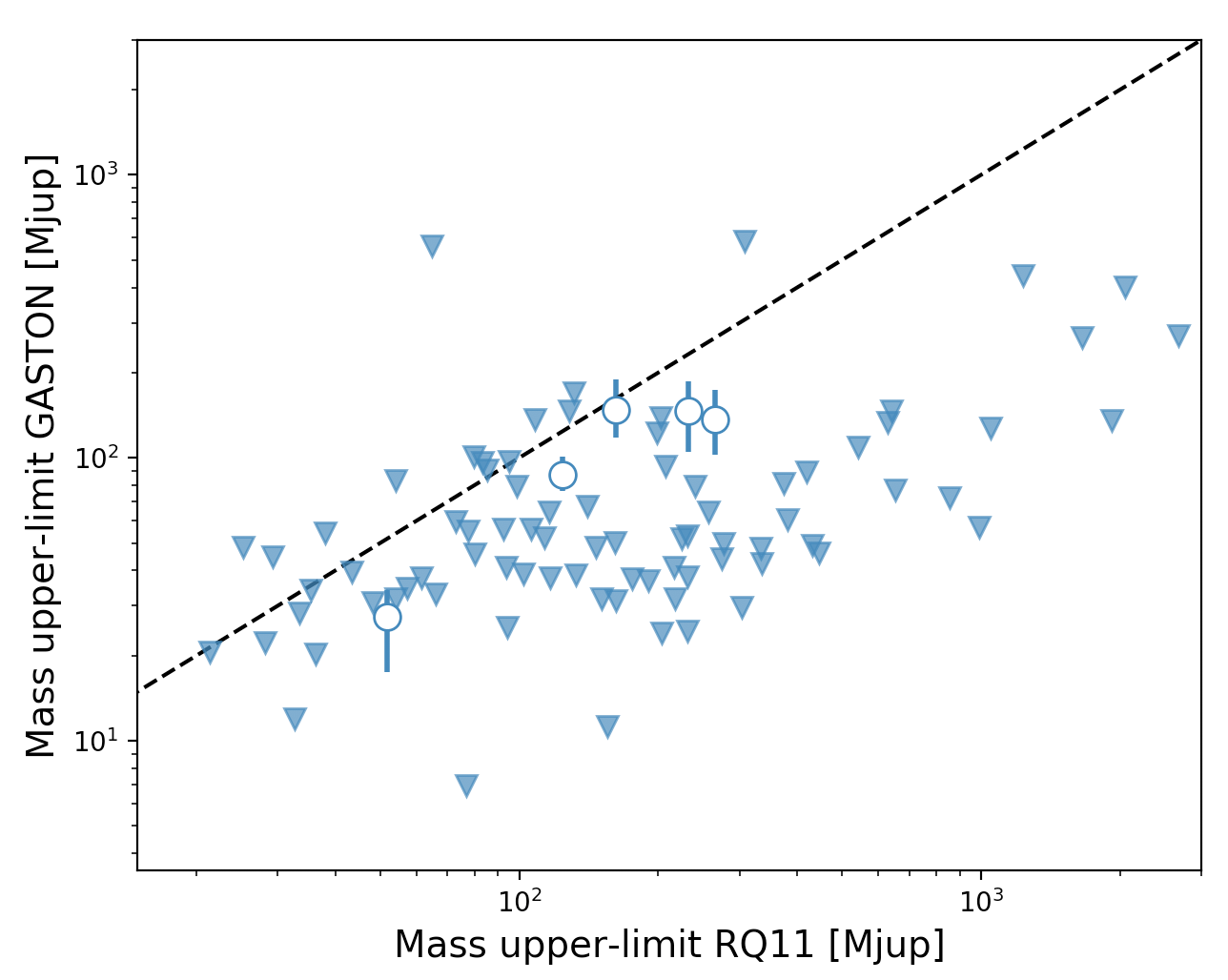
Figure 14: A comparison plot of GASTON mass measurements (open blue circles) and other 3-$\sigma$ upper-limits (plain blue triangles) with Reffert & Quirrenbach (2011), or RQ11, 3-$\sigma$ mass upper-limits for the same companions. The black dashed line represents the relation $M_{3\sigma,\text{GASTON}}$=$M_{3\sigma,\text{RQ11}}$.

Table 10: Comparison of results in the present studies to 1 or 3-$\sigma$ upper-limits published in other articles. Inclinations should be compared modulo $180^{\circ}$ since in the present study the prograde or retrograde orientation of the orbital motion cannot be determined. We present the 1-$\sigma$ confidence interval for the inclinations and masses when they are well-constrained in the present study and obtained with a $\sin I_{c}$ prior distribution on the inclination, and the 3-$\sigma$ limits obtained with a flat prior distribution (Table LABEL:tab:results_nondet_comp) otherwise.

Companion	Reffert & Quirrenbach (2011)		Other publications		Present study
	$I_{c}$	true mass	$I_{c}$	true mass	$I_{c}$	true mass
	(3-$\sigma;\,^{\circ})$	(3-$\sigma$; M${}_{\text{J}}$)	(1-$\sigma;\,^{\circ})$	(1-$\sigma$; M${}_{\text{J}}$)	(1 or 3$\sigma;\,^{\circ})$	(1 or 3$\sigma$; M${}_{\text{J}}$)
Well-constrained mass with GASTON at 1-$\sigma$
30 Ari B b	(3.8,174.8)	$<$162.2			$4.2^{+1.0}_{-0.9}$	$147^{+41}_{-29}$
HD 114762 b	(4.1,176.7)	$<$233.0	$4.87^{+1.11}_{-0.91}$	$141^{+35}_{-28}$	$4.9^{+1.8}_{-0.9}$	$147^{+39}_{-42}$)
HD 141937 b	(11.0,166.2)	$<$51.7			$20.5^{+12.5}_{-4.2}$	$27.4^{+6.8}_{-9.9}$
HD 148427 b	(4.8,176.6)	$<$265			$0.51^{+0.16}_{-0.11}$	$137^{+37}_{-34}$
HD 5388 b	(1.0,179.0)	$<$124.3	178.3${}^{+0.4}_{-0.7}$	62.2$\pm$19.9	$1.4\pm 0.2$	$87^{+14}_{-11}$
3-$\sigma$ limits with GASTON
HD 33636 b	(2.9,176.8)	$<$207.3	4.0$\pm$0.1	142$\pm$11	$>$6.02	$<$93.5
HD 87883 b	(4.9,34.9)	(3.1,21.4)			$>$4.9	$<$21
HD 92788 b	(2.5,178.0)	$<$113.6	6.3 ; (0,22)	45 ; (9,28)	$>$4.0	$<$52
HD 102195 b	(0.0 ,180.0)	—	(72.5,84.79)	0.46$\pm$0.03	$>$0.21	$<$133
HD 128311 c	(7.5,171.1)	$<$25.2	55.950$\pm$14.553	3.789${}^{+0.924}_{-0.432}$	$>$4.0	$<$49
HD 130322 b	(0.0 ,180.0)	—	76${}^{+14}_{-42}$	1.1${}^{+1.0}_{-0.1}$	$>$0.59	$<$108
HD 131664 b	(153.9,171.5)	(42.3,131.6)	55$\pm$33	23${}^{+26}_{-5}$	$>$6.6	$<$170
HD 136118 b	(138,172.7)	$<$95.3	163.1$\pm$3.0	42${}^{+11}_{-18}$	$>$7.25	$<$97
HD 142022 b	(4.2,49.1)	(4.6,102.2)			$>$4.348	$<$38.84
HD 154345 b	(1.7 ,178.1)	$<$32.6	50${}^{+40}_{-26}$	1.2${}^{+1.3}_{-0.4}$	$>$4.7	$<$12
HD 177830 b	(0.9,179.6)	$<$225.2	1.3	55	$>$1	$<$79
HD 181720 b	(0.1 ,3.4)	(6.1,217.9)			$>$0.68	$<$32
HD 190228 b	(2.5,40.8)	(9.1,142.9)	4.3${}^{+1.8}_{-1.0}$	49$\pm$15	$>$1.56	$<$111.4

Besides Reffert & Quirrenbach (2011), we found several other publications of true mass and inclinations for 12 companions. They are summarized on Table 10 and discussed individually below.

HD 5388 b

The mass of this exoplanet candidate was already measured to be 62.2$\pm$19.9 M${}_{\text{J}}$ with Hipparcos measurements (Sahlmann et al. 2011b). Our new mass estimation of 87.02${}^{+13.99}_{-10.80}$ M${}_{\text{J}}$ is 2-$\sigma$ compatible with Sahlmann et al. (2011b) estimation. This companion is thus indeed a likely massive brown dwarf.

HD 33636 b

Bean et al. (2007) rejected the planetary nature of this candidate, with a mass determined in the M-dwarf domain $M$=140$\pm$11 M${}_{\text{J}}$ with an orbital inclination of $\sim$4^∘. Interestingly, the small astrometric excess noise measured by Gaia $\varepsilon_{\text{DR1}}$=0.53 mas leads to a probability for the mass of this companion to be higher than 93.5 M${}_{\text{J}}$ is 0.27%. The mass measurements from Gaia and FGS astrometry are thus incompatible at 3$\sigma$. However, with an inclination of 4^∘, our simulations could produce $\varepsilon_{\text{DR1}}$ smaller than 0.53 mas with a probability of 0.7%. Thus, the Gaia DR1 astrometric excess noise is compatible with Bean et al. (2007) results at 3$\sigma$. The disagreement between the parallax of this measured by FGS and Hipparcos ($\sim$35-36 mas) with the parallax measured by Gaia ($\sim$34) may also explain the small $\varepsilon_{\text{DR1}}$ if part of the orbital motion was wrongly fitted as parallax motion.

HD 92788 b

Han et al. (2001) proposed a true mass of 45 M${}_{\text{J}}$, with an inclination of 6.3^∘ for this Jupiter-mass candidate ($m\sin i$=3.6 M${}_{\text{J}}$) on an Earth-like orbit ($P$=325 days). Simpson et al. (2010) later proposed a derivation of the orbit inclination based on the assumption of coplanarity of the stellar equator and the companion orbit and by measuring the rotation speed of the star compared to its $v\sin i$. This led to a lower mass of 9-28 M${}_{\text{J}}$. This method is however not fully reliable as coplanarity of the stellar equator and the companion orbit is never a robust assumption. Both results are compatible with the 3-$\sigma$ limit that we derived here ($I_{c}$$>$$3.9^{\circ}$, $M_{b}$$<$$54$ M${}_{\text{J}}$) with $\varepsilon_{\text{DR1}}$=0.32 mas. It confirms that this companion is most likely a brown-dwarf if not a massive planet.

HD 102195 b

This companion on a 4-days orbit was determined as planetary by Guilluy et al. (2019) by extracting the emitted spectrum of its atmosphere. They determined a Jovian mass of 0.46 M${}_{\text{J}}$ with an orbit inclination of 72-85^∘. GASTON cannot confirm the planetary nature of HD 102195 b, with a 3-$\sigma$ limit on its mass of 187 M${}_{\text{J}}$ and a minimum inclination of 0.15^∘.

HD 114762 b

Its true mass was already published in Kiefer (2019). The results that we find here for this companion are compatible with those reported in Kiefer (2019) when HD 114762 B is not taken into account, validating that the modifications brought to GASTON (see Section 4) kept the results of such well-behaved case unchanged. The tentative estimation of the mass of this companion obtained by Han et al. (2001) from few Hipparcos points led to an inclination of 4.3^∘ and a companion mass of 145 M${}_{\text{J}}$, in full agreement with our result.

HD 128311 b & c

This system has two known companions $b$ and $c$, with periods of respectively 454 and 924 days, in an almost 2:1 resonance, with minimum masses of 1.5 and 3.2 M${}_{\text{J}}$. The outermost companion $c$ was shown to be most likely planetary by McArthur et al. (2014) using HST/FGS precise astrometry, with an orbit inclination of 55.95$\pm$14.55^∘ and a mass of 3.789${}^{+0.92}_{-0.43}$ M${}_{\text{J}}$. There are no constraint on the inclination or true mass of companion $b$, but an assumed coplanarity with planet $c$ orbit would imply a planetary nature as well with a mass close to 2 M${}_{\text{J}}$. Coplanarity is not generic, and it remains thus possible that planet $c$ is actually circumbinary, possibly leading to an interesting configuration in 2:1 resonance. The non-detection of the astrometric motion of the host star by the Gaia DR1 astrometric excess noise with $\varepsilon_{\text{DR1}}$=0.6 mas puts a 3-$\sigma$ upper-limit on the mass at 46 and 48 M${}_{\text{J}}$ for companions $b$ and $c$. We can therefore exclude a stellar nature for planet $c$ in agreement with McArthur et al. (2014), as well as for object $b$, but it could still be a brown dwarf.

HD 130322 b

As for HD 154345 b, assuming the coplanarity of HD 130322’s equator and companion $b$ orbit, Simpson et al. (2010) proposes a mass of 1.1 M${}_{\text{J}}$ for this companion. The low astrometric excess noise of 0.3 mas for this source allows deriving with GASTON a 3-$\sigma$ upper-limit on the mass of HD 130322 b of 136 M${}_{\text{J}}$. The planetary nature of this object cannot be confirmed here.

HD 131664 b

This 5-years period candidate brown dwarf ($m\sin i$=18 M${}_{\text{J}}$) was characterized using Hipparcos astrometry by Sozzetti & Desidera (2010) and Hipparcos-2 data by Reffert & Quirrenbach (2011). Both found a possible small orbital inclinations for this companion down to $\sim$10-20^∘. Sozzetti & Desidera (2010) could not reject an edge-on inclination while Reffert & Quirrenbach (2011) obtain inclinations smaller than 30^∘ at 3$\sigma$ with a mass of at least 42 M${}_{\text{J}}$. GASTON cannot help settling the true mass of HD 131664 b but constrains its mass to less than 170 M${}_{\text{J}}$ at 3$\sigma$.

HD 136118 b

Using the Hubble Space Telescope Fine Guidance Sensor (HST/FGS), Martioli et al. (2010) could measure the astrometric motion of the F9V star HD 136118. They obtained an inclination of 163$\pm$3^∘ and a true mass for the exoplanet candidate of 42${}^{11}_{-18}$ M${}_{\text{J}}$ instead of the 12 M${}_{\text{J}}$ deduced from RV assuming an orbit seen edge-on. The 3-$\sigma$ upper-limit that we derived with GASTON for the true mass of HD 136118 b is close to the 3-$\sigma$ upper-limit derived from Hipparcos-2 measurements by Reffert & Quirrenbach (2011) about 95-97 M${}_{\text{J}}$. The Gaia DR1 astrometric excess noise of HD 136118 (0.51 mas) is thus compatible with the true astrometric motion $\sim$1.45 mas of the host star due to companion ’b’.

HD 154345 b

This long-period (3325 days) companion is a planet confirmed by Simpson et al. (2010) by measuring the rotation axis angle of the host star. But this conclusion relies on the hypothesis of coplanar orbital and stellar equator planes, which is never guaranteed. Our 3-limit based on $\varepsilon_{\text{DR1}}$=0.35 mas shows that HD 154345 b is indeed a planet with a mass smaller than 11.6 M${}_{\text{J}}$.

HD 177830 b

Its true mass was tentatively determined at 55 M${}_{\text{J}}$, with an inclination of 1.3^∘ by Han et al. (2001) using Hipparcos data. This result is within the 3-$\sigma$ limit that we derived here ($I_{c}$$>$$1.0^{\circ}$, $M_{b}$$<$$79$ M${}_{\text{J}}$). It confirms that the $\varepsilon_{\text{DR1}}$=0.87 mas for this source incorporates a consequent fraction of real astrometric orbital motion.

HD 190228 b

Using Hipparcos astrometry, this companion was previously identified as a brown dwarf with a mass of 67$\pm$29 M${}_{\text{J}}$ (Zucker & Mazeh 2001a). Its mass was then reduced to 49$\pm$18 M${}_{\text{J}}$ and an inclination of 4.3^∘ ​${}^{+1.8}_{-1.0}$ (Sahlmann et al. 2011a). The orbit significance they obtained for this star was 2-3$\sigma$. Using GASTON and a $\sin i$-prior on the inclination, we measure a 1-$\sigma$ upper-limit for the same mass of $<$24 M${}_{\text{J}}$ and a 3-$\sigma$ upper-limit of 111 M${}_{\text{J}}$. The inclination is $>$14^∘ at 1-$\sigma$ and $>$3.2^∘ at 3-$\sigma$. Our result agrees with the most precise measurements of the mass of HD 190228 b, but cannot bring significant improvements. Given the astrometric orbit semi-major axis as large as 2 mas, Gaia will certainly provide the best measurement for this brown-dwarf once the astrometric series will be available.

The global compatibility of the true masses derived with GASTON with the true masses already published for these systems validates the GASTON method and confirms it can lead to better characterize candidate planetary systems.

6.6 An updated mass-period diagram

The masses derived with GASTON allow us to update the mass-period diagram of planet and brown dwarf companions. It is represented in Fig. 15, compared to companions with true mass from the Exoplanet.eu database and massive companions reported in Wilson et al. (2016) and Kiefer et al. (2019). We selected only systems within 60 pc from the Sun, surrounding FGK host stars with masses within 0.52–1.7 M_⊙, with a published inclination measurement. Such systems are objects of extensive surveys (e.g. Sahlmann et al. 2011a, Hébrard et al. 2016, Kiefer et al. 2019) with better observational completion and detection of planets and BD with mass larger than 1 M${}_{\text{J}}$. We include any mass compatible with as much as 150 $M_{\text{J}}$ in order to encompass the surroundings of the substellar domain. We exclude GASTON masses of transiting planets, which are better determined in the Exoplanet.eu database. We also exclude the GASTON mass of candidates which host star RVs have a long-term drift, in order to remove possible bias due to an outer companion. Upper-limits are not represented.

The mass measurements of the present study add new points to the $M$-$P$ diagram in the BD-to-stellar domain at orbital periods larger than 100 days. There still remains blank regions: the BD domain below 100-days period (Kiefer et al. 2019a), the short-period Neptunian desert (Mazeh et al. 2016), and the observationally biased triangular area from short-period Earth-mass planets to long-period Jupiter mass planets.

In the BD domain, the $M$-$P$ distribution presents a strong cut in the region of brown dwarf companions at $\sim$100 days. But below 100 days, several tens of other companions which mass cannot be well-constrained may reside in the BD mass regime. In Fig. 16, we included the 3-$\sigma$ upper-limits derived with GASTON around and in the BD domain. Even then, the region bounded by masses 20-85 M ${}_{\text{J}}$ and periods 0-100 days remains significantly emptier than its surrounding. This tends to confirm the most recent estimation of the brown dwarfs desert boundaries (Ma & Ge 2014, Ranc et al. 2015, Kiefer et al. 2019).

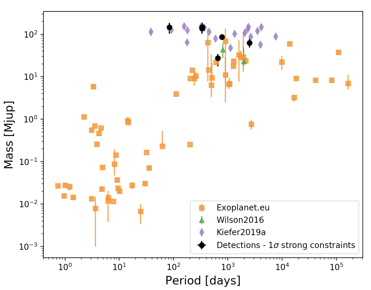
Figure 15: Mass-period diagram from planets up to low-mass M-dwarfs ($\sim$150 M${}_{\text{J}}$). The true masses derived with GASTON for non-transiting planets and systems without RV-drift are represented as black circles. They are compared to the true mass and period of companions in the exoplanet.eu database (orange squares), and of supplementary BD and low-mass M-dwarfs published in Wilson et al. (2016) in green, and Kiefer et al. (2019) in purple. Only systems within 60 pc from the Sun and surrounding FGK host stars (0.52$<$$M_{\star}$$<$$1.7$ M_⊙) are represented.

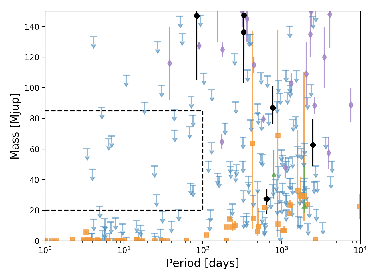
Figure 16: Same diagram as Fig. 15, but focused on the 0-90 M${}_{\text{J}}$ region with a linear scaling of the y-axis and centered on the BD domain. The 3-$\sigma$ upper-limits on mass derived by GASTON are shown as blue downward arrows.

6.7 Star-host metallicity and orbital eccentricity distributions in the BD domain

Brown dwarfs companion stand at the boundary between stellar binaries and giant planets. It remains unknown if some BD companions belong to one or the other population, or if BDs have a main formation channel.

Core-accretion scenarios (Pollack et al. 1996) predict that giant planets are more difficult to form around metal-deficient stars (Ida & Lin 2005) and strong observational evidences show that giant planets indeed occur less frequently about stars with sub-solar metallicity (Fischer & Valenti 2005, Mayor et al. 2011). On the other hand, the formation of stellar binaries by gravitational instability does not depend on the metallicity of the host star and it is expected that binary companions have the same metallicity distribution whatever their mass (Maldonado et al. 2017).

The study of eccentricity distributions in the BD domain by Ma & Ge (2014) revealed the existence of a sharp transition at $\sim$42.5 M${}_{\text{J}}$. Below 42.5 M${}_{\text{J}}$ the eccentricity distribution is consistent with mass-limited eccentricity pumping by planet-planet scattering (Rasio & Ford 1996), and beyond 42.5 M${}_{\text{J}}$ the eccentricity distribution of BD companions is similar to that of binary stars (Halbwachs et al. 2003). A consistent transition at similar mass was found by Maldonado et al. (2017) in the distribution of host star metallicities. The host-star metallicity of BD with a mass $>$42.5 M${}_{\text{J}}$ spans a large range of values from sub-solar to super-solar, while those with mass $<$42.5 M${}_{\text{J}}$ have host-stars metallicities more similar to those of giant exoplanets with a prevalence for metal-rich hosts.

This limiting mass of $\sim$42.5 M${}_{\text{J}}$ could thus be separating low-mass BDs formed like planets by core-accretion from high-mass BDs formed like stars by gravitational instability in molecular clouds.

Here, we add the new GASTON measurements to exoplanet.eu companions, and the published companions in Wilson et al. (2016) and Kiefer et al. (2019a) to obtain metallicity and eccentricity distributions with respect to true masses in Figs. 17 and 18. We select, as in Section 6.6, systems within 60 pc from the Sun, surrounding FGK host stars with masses within 0.52–1.7 M_⊙, and with a published inclination measurement. Metallicity, or [Fe/H], measurements are taken from the exoplanets.org database for the sample studied in the present paper, from exoplanet.eu for the corresponding sample, and from the Wilson et al. (2016) and Kiefer et al. (2019a) for the rest of the considered companions.

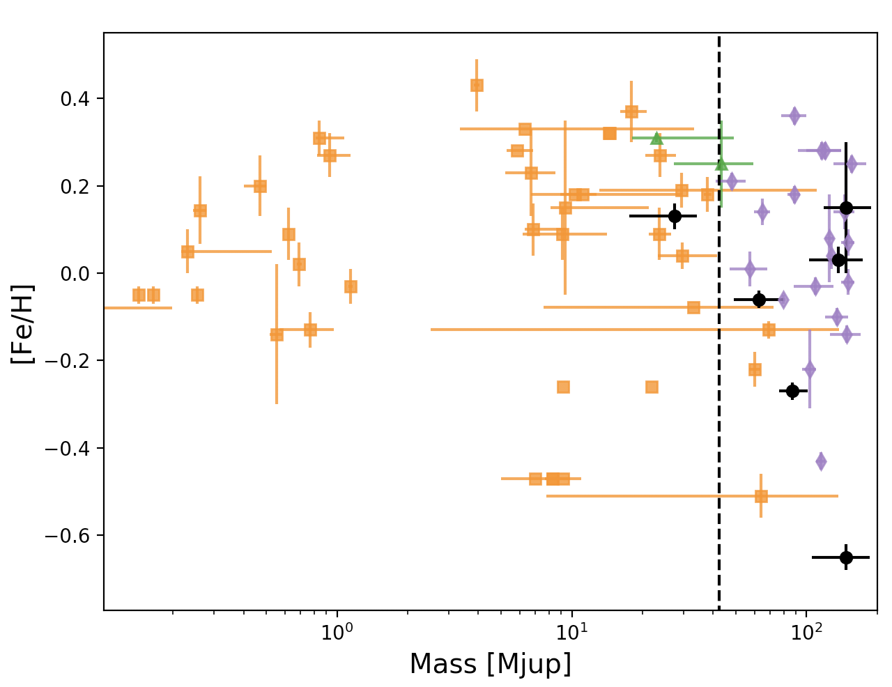
Figure 17: Mass-metallicity diagram from planets up to low-mass M-dwarfs ($\sim$150 M${}_{\text{J}}$). The symbols are the same as in Figure 15. The dashed line indicates the 42.5 M${}_{\text{J}}$ mass-limit derived by Ma & Ge (2014).

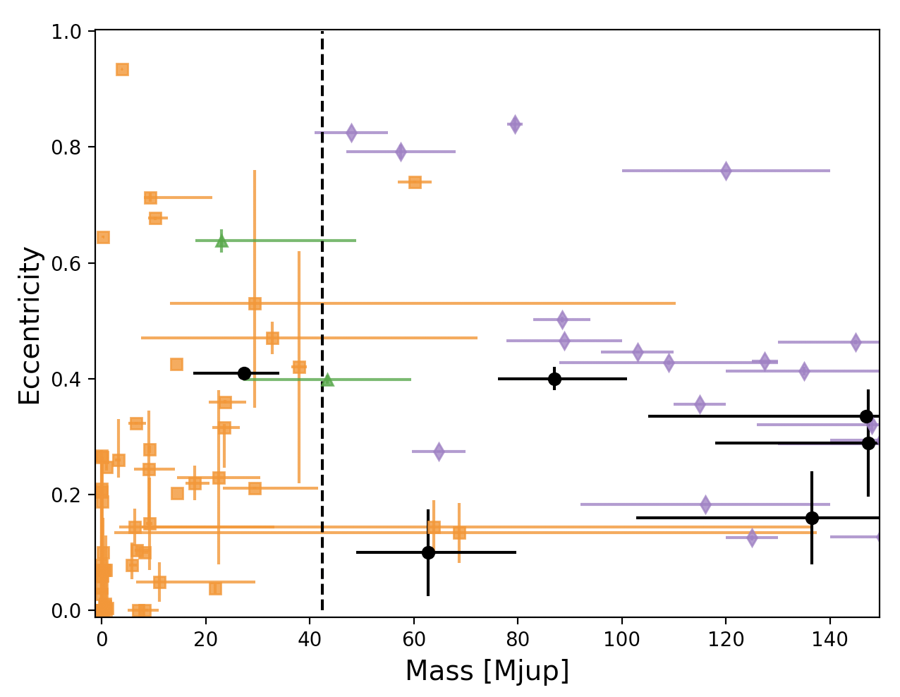
Figure 18: Mass-eccentricity diagram from planets up to low-mass M-dwarfs ($\sim$150 M${}_{\text{J}}$), with a linear scale as in Ma & Ge (2014). The symbols are chosen the same as in Figure 17.

Beyond the brown dwarf domain, metallicity reaches sub-solar values, while giant planets are indeed found preferably around stars with super-solar metallicity. No clear boundary can be derived from the still sparse distribution of measured companion mass, although a transition could be occurring about 50 M${}_{\text{J}}$ in agreement with the 42.5 M${}_{\text{J}}$ found by Maldonado et al. (2017). The distribution of eccentricity with companion mass in Fig. 18 does not exhibit a well-defined transition at 42.5 M${}_{\text{J}}$, as reported in Ma & Ge (2014). Nevertheless, four BD with $M$$>$$45$ M${}_{\text{J}}$ stand above $e$$=$$0.7$ while all BD companions have $e$$<$$0.7$ below $45$ M${}_{\text{J}}$. The eccentricity distribution within our sample thus seems to match with that of Ma & Ge (2014).

Our current sample of exoplanets, BD and low-mass M-dwarf companions around FGK stars at less than 60 pc of the Sun with a true mass measured still need to be populated, but it agrees with previous non-volume limited studies on a transition in the brown dwarf domain at a mass of $\sim$42.5 M${}_{\text{J}}$. This critical mass possibly separates two populations of BD, those formed like stars from those formed like planet and mainly following predictions of the core-accretion scenario.

7 Conclusions

We use the GASTON method developed in Kiefer et al. (2019) & Kiefer (2019) with Gaia DR1 data to determine the true mass of the 911 RV-detected exoplanet candidates published in the exoplanets.org database. Reliable DR1 data were found for the host stars of 755 companions. Among those, a total of 29 companions induce an orbital motion of their host star significant enough to be detected as large astrometric excess noise, constituting a ’detection sample’. With GASTON, an inclination, and thus a true mass could be determined for 8 of them. For the remaining 21 companions we could only constrain an upper-limit on the true mass, with an astrometric motion compatible with the edge-on inclination within measurement noise. For other 227 candidates, the astrometric excess noise is not large enough to imply a firm detection of the astrometric motion of their host star, but it allows deriving an upper-limit on their true mass. They constitute a ’non-detection sample’.

We found that among the detection sample, 30 Ari B b, HD 114762 b, HD 148427 b, HD 5388 b, HD 6718 b, HD 16760 b, and HIP 65891 b are not planets, but brown dwarfs or M-dwarfs. Moreover, we measured a true mass of HD 141937 b, within 9-50 M${}_{\text{J}}$ compatible at 3-$\sigma$ with a planetary nature, altthough more likely a brown-dwarf.

Among the 227 candidates of the non-detection sample, GASTON applied on the small astrometric excess noise measured by Gaia DR1 confirms that 27 exoplanet candidates are indeed planets. The lower-limit on their inclination deduced from the small value of their astrometric excess noise led to an upper-limit on mass below 13.5 M${}_{\text{J}}$ at 3-$\sigma$.

These new measurements populate the mass-period diagram in the BD-to-M-dwarf domain constraining the driest region of the desert of brown-dwarf companions detection, also-known-as the brown-dwarf desert, to orbital periods smaller than 100-days and mass larger than 20 M${}_{\text{J}}$. We thus confirm previous estimates of the period threshold of the brown-dwarf desert, $\sim$100 days, obtained by Ma & Ge (2014) accounting for the true mass of whole set of detected BD companions as of 2014, and Kiefer et al. (2019) analysing the $m\sin i$ distribution of companions to FGK-stars at less than 60 pc from Earth. Moreover, the distributions of eccentricities and metallicities among brown dwarf companions are consistent with a transition from planet-like formation to star-like formation at about 40-50 M${}_{\text{J}}$ (Ma & Ge 2014, Maldonado et al. 2017).

Since GASTON allowed determining companion masses of few tens of M${}_{\text{J}}$ using only preliminary Gaia data products at a precision of $\sim$1 mas, we can rejoice that future orbital solutions from Gaia astrometric time series at a precision of a few 10-100 $\mu$as, will allow measuring the orbital inclination and masses of many RV Jupiter-mass exoplanets and brown dwarfs, as well as new detections among the several billions of sources monitored with Gaia.

Appendix A The magnitude of the companion

To calculate the impact of the light emitted from the companion on the apparent primary semi-major axis, as observed by Gaia, also known as the photocenter semi-major axis, we have to take into account two effects: the emission from the companion (c) itself if not planetary and the star ($\star$) light reflected by the companion towards the observer. We recall the equation of the photocenter semi-major axis given in Kiefer et al. (2019) (see also van de Kamp 1975 for the original calculation):

$$a_{\text{phot}}=(B-\beta)a_{\text{tot}}\qquad\text{with }a_{\text{tot}}=a_{c}+a_{\star}$$ (1)

We introduced the luminosity fraction $\beta$=$L_{c}/(L_{c}+L_{\star})$ and the mass fraction $B$=$q/(1+q)$ with $q$=$M_{c}/M_{\star}$ the mass ratio. The key-parameter here is the luminosity fraction.

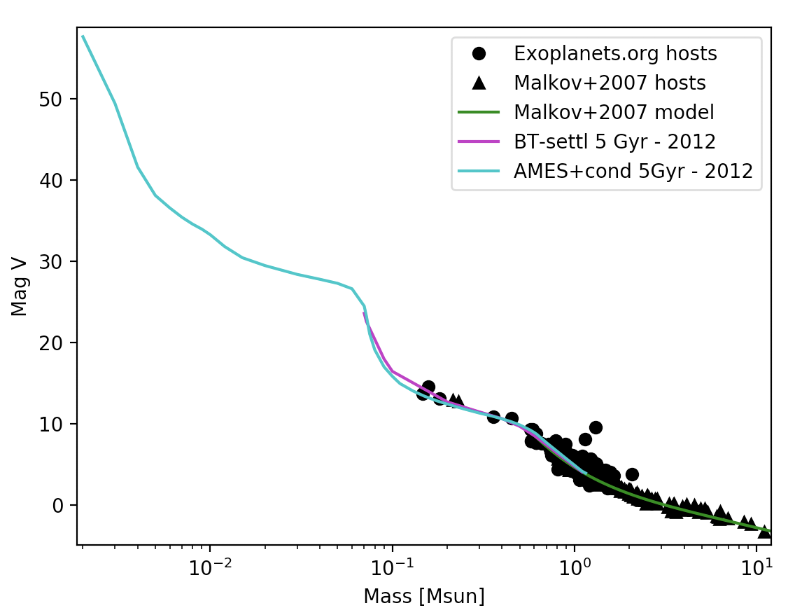
Figure 19: Absolute visual magnitude of emitted light against mass from low-mass brown-dwarf up to massive stars. Data are taken from the Exoplanets.org catalog and Malkov et al. (2007). Solid lines are models, as presented in the legend.

In order to calculate the emitted $V$-magnitude of the components, we use different empirical models. We use the given $V$ magnitude as an approximation of the $G$ magnitude. Since only the $\delta G$ is important for our study, we do not expect strong deviations due to this approximation. They are listed below and presented on Fig. 19, compared to published data from exoplanets.org and Malkov (2007) in the Johnson $V$-band:

• Allard et al. (2012) AMES-cond isochrone at 5 Gyr, for the BD-to-dM regime,

• BT-Settl (Allard et al. 2012, and references therein) isochrone at 5 Gyr, for the stellar regime up to 1.1 M_⊙,

• Malkov (2007) empirical model above 1.1 M_⊙ up to 10 M_⊙.

Only visual magnitudes for objects with mass larger than 0.1 M_⊙ could be found in the literature, due to the difficulty for observing faint objects such as brown dwarfs and exoplanets in the optical band. Therefore, we can only assess the validity of the $V$-mag models in the stellar domain and we will assume their validity in the $G$-band down to the planetary domain owing moreover to the relative compatibility of the AMES-cond models with observations in the infrared (Chabrier et al. 2000, Baraffe et al. 2003, Allard et al. 2012). The BT-settl model seems more accurate than AMES-cond in the IR for massive brown-dwarfs (Allard et al. 2012), but it does not give magnitudes for objects with mass below 0.75 M_⊙. In order to insure continuity of the mass-magnitude relation we prefer using the AMES-cond model from masses of 0.1 M_⊙ down to 10 M${}_{\text{J}}$.

For the reflected light, we calculate the mean reflection along an entire orbit. For the whole domain from planets to stars, we assume the body is a Lambertian sphere with a typical Bond albedo of 0.3. The radius of the sphere is related to the mass of the body. There is no continuous exact law $R$=$f(M)$ on the whole planet-to-star domain, with a wide diversity of densities for planets and also for stars if we account for (sub-)giants stars. However, for the sake of continuousness and simplicity, we will assume a common continuous law relating the radius of a body to its mass. This will avoid issues with gaps in the MCMC and allow us to derive well-behaved posterior distributions. This law is established using several segments and is presented in Fig. 20:

• Low-mass planets, up to 0.5 M_J with the empirical relations of Bashi et al. (2017),

• Jovian-mass planets and brown-dwarfs up to 0.1 M_⊙ stars along an AMES-cond isochrone at 5 Gyr (Allard et al. 2012),

• Low-mass stars from 0.1 to 1.1 M_⊙ with the BT-settl model (Allard et al. 2012, and references therein) along an isochrone at 5 Gyr,

• More massive stars up to 10 M_⊙ with the empirical $R\propto M^{0.57}$ relationship (e.g. Demircan & Kahraman 1991, Torres et al. 2010).

Taking into account emission and reflection from the companion, we can calculate magnitude differences between the primary and the companion for different values of their mass and for different companion’s orbit semi-major axis. This is plotted on Fig. 21. The net impact on the apparent primary semi-major axis can be measured by comparing the photocenter semi-major axis to the primary semi-major axis. This is presented on Fig. 22. In general the semi-major axis of the photocenter orbit decreases with increasing contribution of the companion in the total luminosity of the system.

In the stellar regime, the impact of the companion starts to be significant on the apparent primary semi-major axis for companion masses larger than about 20% of the primary star mass. For a primary of mass 0.5 M_⊙ the magnitude of the secondary has a measurable effect for a mass larger than about 0.1 M_⊙. If the secondary is too luminous compared to the primary, the semi-major axis of the photocenter can even reach 0. However this effect remains hidden in the present study, because we impose that the companion be dark with ($\Delta V$$>$$2.5$).

In the planetary mass regime on the other hand, the impact of the companion on the photocenter can be strong if the semi-major axis of the companion orbit is smaller than 0.5 au and the mass ratio $q$=$M_{c}/M_{\star}$$\sim$$10^{-5}-10^{-3}$. The impact is stronger for earlier primaries. This is due to the shortening of the primary star orbit with decreasing companion mass, while the companion radius is relatively constant about 1 R${}_{\text{J}}$ down to a few fractions of Jupiter mass (Bashi et al. 2017). In this regime, the astrometric motion of the system observed from Earth, although of small extent, can actually follow the motion of the companion rather than that of the stellar host. This happens precisely when the luminosity ratio $L_{c}/L_{\star}$$>$$q$.

Nevertheless, this effect will not have a strong role in the present study, because $q$$\sim$$10^{-5}-10^{-3}$ with $a_{c}$$<$$0.5$ a.u. implies $a_{\star}$$\ll$$a_{c}$ and $a_{\text{ph}}$$<$$10^{-3}$ a.u. In the worst case scenario, it could only lead at most to an astrometric motion of $\sim$0.5 mas if the parallax is $\sim$500 mas. This is well below the detection thresholds ($\varepsilon_{\text{thresh,prim}}$=0.85 mas and $\varepsilon_{\text{thresh,second}}$=1.2 mas) defined in Section 3.5 and this situation is thus undetectable within the diverse noises accounted for in Gaia measurements. However, it will be an important effect to account for in future analysis of Gaia time series when this precision will be reached. Neglecting it might lead to strongly underestimate the star semi-major axis, and thus the mass of the companion.

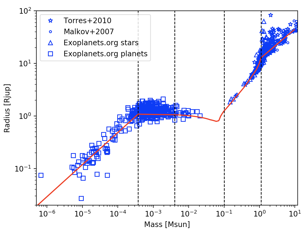
Figure 20: Radius against mass from terrestrial mass planets up to massive stars. Data are taken from the Exoplanets.org catalog, Malkov et al. (2007) and Torres et al. (2010). The red solid line represents the continuous model, comprised of Bashi et al. (2017) from 10^-6 to 0.004 M_⊙, Baraffe et al. (2003) from 0.004 to 0.1 M_⊙, BT-settl from 0.1 to 1.1 M_⊙ and the empirical relation $R$$\propto$$M^{0.57}$ above 1.1 M_⊙ (e.g. Demircan 1997).

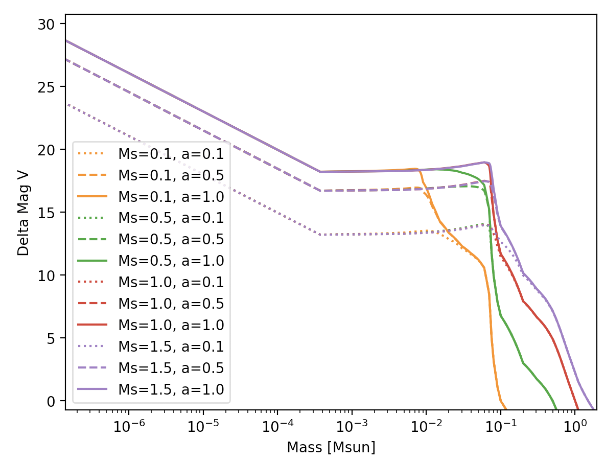
Figure 21: The adopted continuous model of $\Delta V$ with respect to the mass ratio. On this plot, the primary is assumed with a mass ranging from 0.1 to 1.5 M_⊙, and the secondary is a Lambertian sphere with average Bond albedo of 0.3 on an orbit with semi-major axis between 0.1 and 1 au.

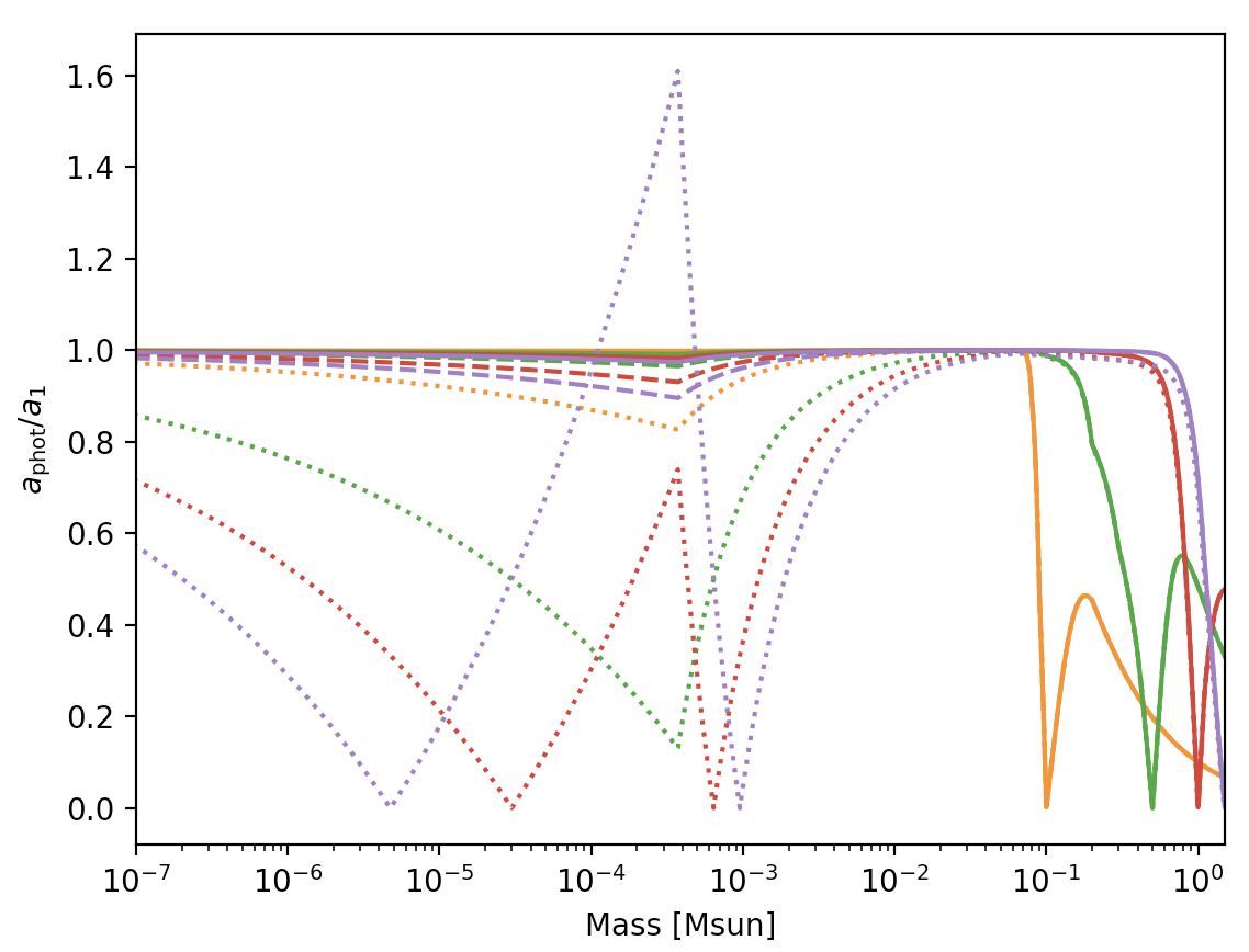
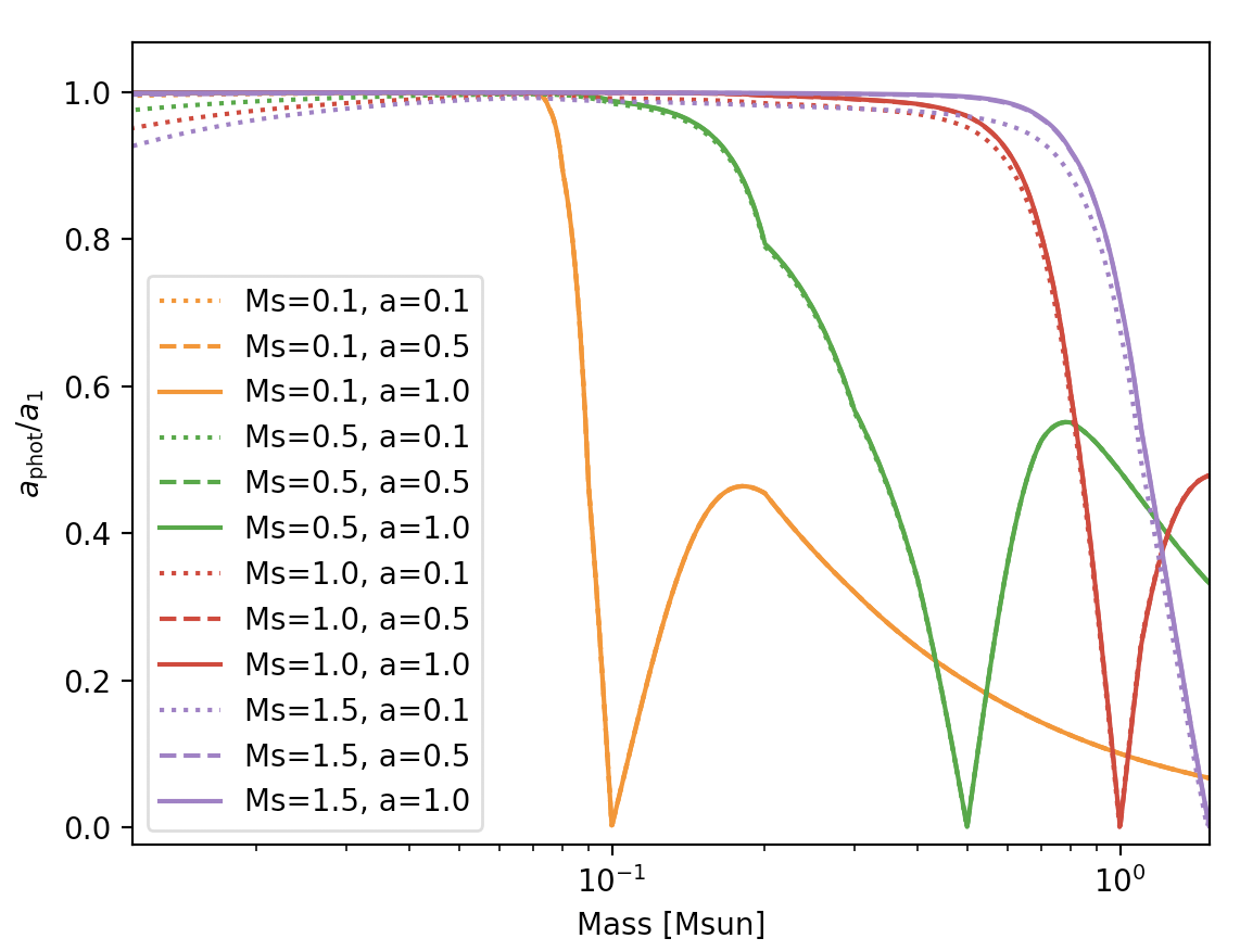
Figure 22: The effect of emitted and reflected light by the secondary companion on the photocenter semi-major axis. Top: on the full mass ratio range. Bottom: beyond $M$=0.1 M_⊙. Captions are identifical in the two panels.

Appendix B Complementary tables of GASTON results for the non-detection sample

Table 11: List of the 227 selected planets in the non-detection sample. Where uncertainties are missing we assume 10% errors on the corresponding parameter. The parallax with uncertainties are all taken from the DR1, while those without uncertainties are taken from SIMBAD.

RV data													Gaia DR1 data
Name	$P$	$m\sin i$	$K$	$e$	$\omega$	$T_{p}$	$M_{\star}$	$a_{p}$	$\pi$	$a_{\star}\sin i$	Transit	Drift	$\varepsilon_{\text{DR1}}$	$N_{\text{pts}}$	$N_{\text{FoV}}$	Gaia	Duplicate
	(days)	(M${}_{\text{J}}$)	(m s-1)		(∘)	-2,450,000	($M_{\odot}$)	(au)	(mas)	(mas)	flag	flag	(mas)			dataset	source
8 UMi b	93.4$\pm$4.5	1.52$\pm$0.15	46.1$\pm$4.0	0.060$\pm$0.090	91$\pm$85	4108$\pm$23	1.80$\pm$0.10	0.490$\pm$0.018	6.14$\pm$0.21	0.00243$\pm$0.00030	n	n	0.26	68	16	1	n
BD -06 1339 b	3.87280$\pm$0.00040	0.0268$\pm$0.0038	4.40$\pm$0.60	0	90	5220.50$\pm$0.10	0.70	0.043	49.78$\pm$0.28	0.000078	n	n	0.52	70	9	1	n
BD -06 1339 c	125.94$\pm$0.44	0.168$\pm$0.054	9.1$\pm$2.9	0.31$\pm$0.11	41$\pm$55	5265$\pm$18	0.70	0.44	49.78$\pm$0.28	0.0050	n	n	0.52	70	9	1	n
BD -08 2823 b	5.600$\pm$0.020	0.0459$\pm$0.0032	6.50$\pm$0.10	0.15$\pm$0.15	30$\pm$100	4637.7$\pm$1.6	0.740$\pm$0.070	0.0558$\pm$0.0018	24.28$\pm$0.24	0.0000803$\pm$0.0000098	n	n	0.40	59	9	1	n
BD -08 2823 c	237.6$\pm$1.5	0.328$\pm$0.033	13.4$\pm$1.0	0.190$\pm$0.090	127$\pm$21	4193$\pm$13	0.740$\pm$0.070	0.679$\pm$0.022	24.28$\pm$0.24	0.00698$\pm$0.00099	n	n	0.40	59	9	1	n
BD -10 3166 b	3.48777$\pm$0.00011	0.430$\pm$0.017	60.9$\pm$1.4	0.019$\pm$0.021	334	1171.22$\pm$0.66	0.920$\pm$0.035	0.04378$\pm$0.00056	12.17$\pm$0.45	0.000238$\pm$0.000016	n	n	0.28	77	11	1	n
BD -11 4672 b	1667$\pm$32	0.538$\pm$0.044	13.4$\pm$1.0	0.050$\pm$0.050	231$\pm$110	5899$\pm$42	0.571$\pm$0.014	2.283$\pm$0.035	36.72$\pm$0.26	0.0754$\pm$0.0066	n	n	0.40	53	6	1	n
BD +14 4559 b	268.94$\pm$0.99	1.52$\pm$0.19	55.2$\pm$2.3	0.290$\pm$0.030	87.6$\pm$7.9	3293.7$\pm$6.3	0.86$\pm$0.15	0.775$\pm$0.045	20.10$\pm$0.24	0.0263$\pm$0.0058	n	n	0.28	35	5	1	n
BD +15 2375 b	153.22$\pm$0.44	1.06$\pm$0.10	38.3$\pm$1.6	0.00$\pm$0.13	55$\pm$128	7680$\pm$665	1.08$\pm$0.14	0.575$\pm$0.025	1.64$\pm$0.50	0.00088$\pm$0.00031	n	n	0.59	87	11	1	n
BD +20 2457 b	379.6$\pm$2.0	11.9$\pm$1.6	322.4$\pm$9.6	0.150$\pm$0.030	208$\pm$22	4677$\pm$28	1.06$\pm$0.21	1.046$\pm$0.069	0.40$\pm$0.41	0.0044$\pm$0.0047	n	n	0.35	52	6	1	n
BD +20 2457 c	622$\pm$10	6.90$\pm$0.97	160.0$\pm$7.2	0.180$\pm$0.060	126$\pm$17	3867$\pm$28	1.06$\pm$0.21	1.454$\pm$0.097	0.40$\pm$0.41	0.0036$\pm$0.0038	n	n	0.35	52	6	1	n
HD 100777 b	383.7$\pm$1.2	1.165$\pm$0.083	34.90$\pm$0.80	0.360$\pm$0.020	202.7$\pm$3.0	3456.2$\pm$2.3	1.00$\pm$0.10	1.033$\pm$0.035	20.26$\pm$0.27	0.0233$\pm$0.0030	n	n	0.55	122	18	1	n
HD 10180 c	5.75962$\pm$0.00028	0.0415$\pm$0.0020	4.54$\pm$0.15	0.077$\pm$0.033	279$\pm$44	4001	1.060$\pm$0.050	0.0641$\pm$0.0010	25.73$\pm$0.22	0.0000617$\pm$0.0000043	n	n	0.47	140	17	1	n
HD 10180 d	16.3567$\pm$0.0043	0.0377$\pm$0.0024	2.93$\pm$0.16	0.143$\pm$0.058	292$\pm$26	4005	1.060$\pm$0.050	0.1286$\pm$0.0020	25.73$\pm$0.22	0.0001122$\pm$0.0000092	n	n	0.47	140	17	1	n
HD 10180 e	49.747$\pm$0.024	0.0798$\pm$0.0043	4.25$\pm$0.18	0.065$\pm$0.035	174$\pm$60	4009	1.060$\pm$0.050	0.2699$\pm$0.0042	25.73$\pm$0.22	0.000499$\pm$0.000037	n	n	0.47	140	17	1	n
HD 10180 f	122.72$\pm$0.20	0.0743$\pm$0.0052	2.95$\pm$0.18	0.133$\pm$0.066	265$\pm$144	4028	1.060$\pm$0.050	0.4928$\pm$0.0078	25.73$\pm$0.22	0.000849$\pm$0.000073	n	n	0.47	140	17	1	n
HD 10180 g	602$\pm$11	0.0674$\pm$0.0094	1.56$\pm$0.21	0	90	4043	1.060$\pm$0.050	1.423$\pm$0.028	25.73$\pm$0.22	0.00222$\pm$0.00033	n	n	0.47	140	17	1	n
HD 10180 h	2248$\pm$104	0.206$\pm$0.016	3.11$\pm$0.21	0.151$\pm$0.072	184$\pm$57	3619	1.060$\pm$0.050	3.42$\pm$0.12	25.73$\pm$0.22	0.0163$\pm$0.0016	n	n	0.47	140	17	1	n
HD 101930 b	70.46$\pm$0.18	0.299$\pm$0.015	18.10$\pm$0.40	0.110$\pm$0.020	251$\pm$11	3145.0$\pm$2.0	0.740$\pm$0.050	0.3020$\pm$0.0068	33.51$\pm$0.28	0.00391$\pm$0.00034	n	n	0.51	98	14	1	n
HD 102195 b	4.11378$\pm$0.00056	0.453$\pm$0.021	63.0$\pm$2.0	0	0	3895.960$\pm$0.030	0.87	0.048	34.02$\pm$0.26	0.00081	n	n	0.51	158	20	1	n
HD 102329 b	778.1$\pm$7.5	4.48$\pm$0.39	84.8$\pm$3.2	0.211$\pm$0.042	178$\pm$10	5096$\pm$30	1.30$\pm$0.15	1.807$\pm$0.070	4.36$\pm$0.30	0.0259$\pm$0.0043	n	n	0.47	71	10	1	n
HD 104067 b	55.806$\pm$0.049	0.186$\pm$0.014	11.56$\pm$0.75	0	90	4043.15$\pm$0.56	0.791$\pm$0.020	0.2643$\pm$0.0022	48.90$\pm$0.27	0.00290$\pm$0.00023	n	n	0.52	278	36	1	n
HD 108147 b	10.8985$\pm$0.0045	0.258$\pm$0.067	25.1$\pm$6.1	0.53$\pm$0.12	308$\pm$24	828.86$\pm$0.76	1.171$\pm$0.021	0.10140$\pm$0.00062	25.84$\pm$0.31	0.00055$\pm$0.00014	n	n	0.78	116	20	1	n
HD 108863 b	443.4$\pm$4.2	2.77$\pm$0.16	45.2$\pm$1.7	0.000$\pm$0.050	177$\pm$60	5516$\pm$70	2.08$\pm$0.14	1.453$\pm$0.034	5.85$\pm$0.30	0.0108$\pm$0.0011	n	n	0.80	203	24	1	n
HD 108874 b	394.48$\pm$0.60	1.290$\pm$0.057	37.3$\pm$1.1	0.128$\pm$0.022	219.4$\pm$9.3	4045$\pm$49	0.950$\pm$0.031	1.035$\pm$0.011	16.87$\pm$0.24	0.0226$\pm$0.0013	n	n	0.56	226	26	1	n
HD 108874 c	1680$\pm$24	1.028$\pm$0.054	18.90$\pm$0.72	0.273$\pm$0.040	10$\pm$11	2797$\pm$49	0.950$\pm$0.031	2.719$\pm$0.039	16.87$\pm$0.24	0.0474$\pm$0.0031	n	n	0.56	226	26	1	n
HD 109246 b	68.27$\pm$0.13	0.768$\pm$0.064	38.2$\pm$1.6	0.120$\pm$0.040	235$\pm$29	4824.6$\pm$4.7	1.01$\pm$0.11	0.328$\pm$0.012	14.68$\pm$0.22	0.00350$\pm$0.00050	n	n	0.42	122	17	1	n
HD 109271 b	7.85430$\pm$0.00090	0.0547$\pm$0.0053	5.60$\pm$0.50	0.250$\pm$0.080	-64$\pm$20	5719.1$\pm$3.6	1.047$\pm$0.024	0.07852$\pm$0.00060	17.63$\pm$0.30	0.0000690$\pm$0.0000070	n	n	0.46	94	11	1	n
HD 109271 c	30.930$\pm$0.020	0.0772$\pm$0.0069	4.90$\pm$0.40	0.150$\pm$0.090	4$\pm$120	5733.0$\pm$8.0	1.047$\pm$0.024	0.1958$\pm$0.0015	17.63$\pm$0.30	0.000243$\pm$0.000023	n	n	0.46	94	11	1	n
HD 109749 b	5.2400$\pm$0.0020	0.275$\pm$0.016	28.30$\pm$0.60	0	0	3013.55$\pm$0.14	1.21$\pm$0.10	0.0629$\pm$0.0017	15.95$\pm$0.30	0.000217$\pm$0.000023	n	n	0.54	71	10	1	n
HD 111232 b	1143$\pm$14	6.84$\pm$0.25	159.3$\pm$2.3	0.200$\pm$0.010	98.0$\pm$6.0	1230$\pm$20	0.78	1.969$\pm$0.016	34.94$\pm$0.22	0.576$\pm$0.022	n	n	0.29	106	19	1	n
HD 114729 b	1114$\pm$15	0.945$\pm$0.073	18.8$\pm$1.3	0.167$\pm$0.055	93$\pm$30	520$\pm$72	0.998$\pm$0.024	2.102$\pm$0.025	26.53$\pm$0.26	0.0504$\pm$0.0042	n	n	0.64	81	11	1	n
HD 11506 b	1405$\pm$45	4.73$\pm$0.34	80.0$\pm$3.0	0.30$\pm$0.10	262$\pm$19	3603$\pm$102	1.190$\pm$0.090	2.602$\pm$0.086	19.90$\pm$0.29	0.197$\pm$0.022	n	n	0.56	104	17	1	n
HD 11506 c	223.60$\pm$0.60	0.360$\pm$0.020	12.50$\pm$0.70	0.240$\pm$0.050	272$\pm$15	4127.0$\pm$9.0	1.240$\pm$0.020	0.7746$\pm$0.0044	19.90$\pm$0.29	0.00427$\pm$0.00026	n	n	0.56	104	17	1	n
HD 117207 b	2597$\pm$41	1.819$\pm$0.089	26.60$\pm$0.93	0.144$\pm$0.035	73$\pm$16	630$\pm$128	1.031$\pm$0.043	3.735$\pm$0.065	30.84$\pm$0.25	0.194$\pm$0.013	n	n	0.45	69	9	1	n
HD 117618 b	25.827$\pm$0.019	0.177$\pm$0.035	12.8$\pm$2.2	0.42$\pm$0.17	254$\pm$19	832.2$\pm$1.6	1.069$\pm$0.032	0.1748$\pm$0.0017	26.20$\pm$0.24	0.00072$\pm$0.00014	n	n	0.27	52	11	1	n
HD 12484 b	58.830$\pm$0.080	2.98$\pm$0.14	155.0$\pm$5.0	0.070$\pm$0.030	-35$\pm$40	6699.0$\pm$5.0	1.010$\pm$0.030	0.2970$\pm$0.0030	20.53$\pm$0.93	0.0172$\pm$0.0012	n	n	0.38	36	4	1	n
HD 125595 b	9.6737$\pm$0.0039	0.0417$\pm$0.0043	4.79$\pm$0.47	0	90	4435.23$\pm$0.15	0.756$\pm$0.017	0.08094$\pm$0.00061	35.38$\pm$0.28	0.000151$\pm$0.000016	n	n	0.41	63	13	1	n
HD 125612 b	559.4$\pm$1.3	3.07$\pm$0.14	79.8$\pm$2.2	0.459$\pm$0.013	41.5$\pm$1.6	4894.8$\pm$2.4	1.100$\pm$0.060	1.372$\pm$0.025	17.52$\pm$0.30	0.0640$\pm$0.0049	n	n	0.45	36	4	1	n
HD 125612 c	4.15474$\pm$0.00052	0.058$\pm$0.010	7.2$\pm$1.2	0.27$\pm$0.12	104$\pm$23	4420.17$\pm$0.23	1.100$\pm$0.060	0.05221$\pm$0.00095	17.52$\pm$0.30	0.0000461$\pm$0.0000087	n	n	0.45	36	4	1	n
HD 12661 b	262.709$\pm$0.083	2.34$\pm$0.10	73.56$\pm$0.56	0.3768$\pm$0.0077	296.0$\pm$1.5	4152.75$\pm$0.87	1.136$\pm$0.072	0.838$\pm$0.018	26.36$\pm$0.22	0.0434$\pm$0.0035	n	n	0.34	89	10	1	n
HD 12661 c	1708$\pm$14	1.949$\pm$0.092	30.41$\pm$0.62	0.031$\pm$0.022	165	6153.42$\pm$0.87	1.136$\pm$0.072	2.918$\pm$0.064	26.36$\pm$0.22	0.126$\pm$0.010	n	n	0.34	89	10	1	n
HD 126614 A b	1244$\pm$17	0.386$\pm$0.044	7.30$\pm$0.70	0.41$\pm$0.10	243$\pm$19	3808$\pm$52	1.145$\pm$0.028	2.368$\pm$0.029	13.44$\pm$0.35	0.0102$\pm$0.0012	n	n	0.75	62	9	1	n
HD 128311 b	454.2$\pm$1.6	1.46$\pm$0.15	46.5$\pm$4.5	0.345$\pm$0.049	63$\pm$16	3835$\pm$11	0.8280$\pm$0.0100	1.0859$\pm$0.0051	61	0.11	n	n	0.60	52	6	2	n
HD 128311 c	923.8$\pm$5.3	3.25$\pm$0.16	78.8$\pm$2.6	0.230$\pm$0.058	28$\pm$15	6987$\pm$41	0.8280$\pm$0.0100	1.7432$\pm$0.0097	61	0.40	n	n	0.60	52	6	2	n
HD 130322 b	10.70850$\pm$0.00030	1.043$\pm$0.040	108.3$\pm$2.0	0.011$\pm$0.015	145$\pm$77	3995.0$\pm$2.3	0.836$\pm$0.015	0.08957$\pm$0.00054	31	0.0033	n	n	0.30	70	9	2	n
HD 131496 b	883$\pm$29	2.24$\pm$0.18	35.0$\pm$2.1	0.163$\pm$0.073	22$\pm$40	6040$\pm$100	1.61$\pm$0.12	2.111$\pm$0.070	7.25$\pm$0.25	0.0204$\pm$0.0024	n	n	0.38	69	9	1	n
HD 131664 b	1951$\pm$41	18.3$\pm$1.3	360$\pm$22	0.6380$\pm$0.0020	149.7$\pm$1.0	2060$\pm$41	1.100$\pm$0.030	3.154$\pm$0.053	19.13$\pm$0.26	0.960$\pm$0.076	n	n	0.50	77	11	1	n
HD 13189 b	471.6$\pm$6.0	7.1$\pm$1.0	173.3$\pm$9.8	0.270$\pm$0.060	161$\pm$12	2328$\pm$20	1.17$\pm$0.23	1.249$\pm$0.083	2.10$\pm$0.23	0.0152$\pm$0.0042	n	n	0.29	41	5	1	n
HD 133131 A b	649.0$\pm$3.0	1.421$\pm$0.062	36.52$\pm$0.93	0.330$\pm$0.030	16.0$\pm$4.7	2327$\pm$23	0.95	1.4	19	0.040	n	n	0.36	77	22	2	n
HD 136118 b	1187.3$\pm$2.4	11.68$\pm$0.42	210.7$\pm$2.5	0.338$\pm$0.015	319.9$\pm$2.1	2999.5$\pm$2.3	1.191$\pm$0.025	2.326$\pm$0.017	19.22$\pm$0.27	0.419$\pm$0.019	n	n	0.51	82	13	1	n
HD 137388 b	330.0$\pm$3.0	0.228$\pm$0.029	7.94$\pm$0.88	0.36$\pm$0.12	86$\pm$29	5209$\pm$25	0.86	0.89	24.79$\pm$0.22	0.0056	n	n	0.36	87	16	1	n
HD 13931 b	4218$\pm$388	1.88$\pm$0.14	23.3$\pm$1.4	0.020$\pm$0.035	290$\pm$78	4494$\pm$904	1.022$\pm$0.021	5.15$\pm$0.32	21.39$\pm$0.24	0.193$\pm$0.019	n	n	0.37	70	11	1	n
HD 142022 b	1928$\pm$46	4.5$\pm$3.3	92$\pm$66	0.53$\pm$0.20	170.0$\pm$9.0	941$\pm$75	0.90	2.927$\pm$0.047	29.13$\pm$0.22	0.40$\pm$0.29	n	n	0.32	101	16	1	n
HD 142415 b	386.3$\pm$1.6	1.662$\pm$0.093	51.3$\pm$2.3	0.50	255.0$\pm$4.0	1519.0$\pm$4.0	1.065$\pm$0.045	1.060$\pm$0.015	28.04$\pm$0.26	0.0443$\pm$0.0032	n	n	0.57	158	23	1	n
HD 143105 b	2.19740$\pm$0.00030	1.213$\pm$0.063	144.0$\pm$2.6	0.000$\pm$0.035	90	6531.3440$\pm$0.0070	1.51$\pm$0.11	0.03795$\pm$0.00092	21.30$\pm$0.21	0.000620$\pm$0.000058	n	n	0.29	105	19	1	n
HD 145377 b	103.95$\pm$0.13	5.78$\pm$0.22	242.7$\pm$4.6	0.307$\pm$0.017	138.1$\pm$2.8	4635.40$\pm$0.60	1.1	0.44933$\pm$0.00037	18.95$\pm$0.25	0.0420$\pm$0.0017	n	n	0.47	152	19	1	n
HD 145934 b	2730$\pm$100	2.28$\pm$0.28	22.9$\pm$2.6	0.053$\pm$0.058	215$\pm$62	1430$\pm$370	1.75$\pm$0.10	4.60$\pm$0.15	4.16$\pm$0.24	0.0239$\pm$0.0036	n	n	0.43	125	19	1	n
HD 147018 b	44.2360$\pm$0.0080	2.127$\pm$0.076	145.3$\pm$1.7	0.4686$\pm$0.0081	336.0$\pm$1.2	4459.49$\pm$0.10	0.927$\pm$0.031	0.2387$\pm$0.0027	24.77$\pm$0.25	0.01295$\pm$0.00066	n	n	0.37	166	22	1	n
HD 147018 c	1008$\pm$18	6.59$\pm$0.29	141.2$\pm$4.1	0.133$\pm$0.011	226.9$\pm$6.9	5301$\pm$22	0.927$\pm$0.031	1.918$\pm$0.031	24.77$\pm$0.25	0.323$\pm$0.019	n	n	0.37	166	22	1	n
HD 148156 b	1027$\pm$28	0.848$\pm$0.069	17.5$\pm$1.0	0.520$\pm$0.065	35$\pm$14	4707$\pm$20	1.2	2.1	17.50$\pm$0.30	0.025	n	n	0.73	151	21	1	n
HD 149143 b	4.0720$\pm$0.0070	1.328$\pm$0.078	149.6$\pm$3.0	0.016$\pm$0.010	0	3483.9$\pm$1.2	1.20$\pm$0.10	0.0530$\pm$0.0015	13.45$\pm$0.25	0.000754$\pm$0.000081	n	n	0.33	75	12	1	n
HD 152581 b	689$\pm$13	1.51$\pm$0.15	36.6$\pm$1.8	0.00$\pm$0.11	321$\pm$90	5320$\pm$190	0.93$\pm$0.12	1.489$\pm$0.067	5.96$\pm$0.27	0.0138$\pm$0.0024	n	n	0.45	98	13	1	n
HD 153950 b	499.4$\pm$3.6	2.74$\pm$0.11	69.2$\pm$1.2	0.340$\pm$0.021	308.2000$\pm$0.0010	4502.0$\pm$4.3	1.120$\pm$0.030	1.279$\pm$0.013	20.82$\pm$0.35	0.0622$\pm$0.0032	n	n	0.84	60	7	1	n
HD 154345 b	3342$\pm$93	0.957$\pm$0.061	14.03$\pm$0.75	0.044$\pm$0.045	68	2831$\pm$334	0.893$\pm$0.038	4.212$\pm$0.098	54.76$\pm$0.22	0.236$\pm$0.019	n	n	0.35	104	18	1	n
HD 155233 b	885$\pm$63	1.99$\pm$0.57	32.2$\pm$8.7	0.03$\pm$0.10	95$\pm$90	5112$\pm$412	1.50$\pm$0.20	2.07$\pm$0.13	13	0.035	n	n	0.70	72	10	2	n
HD 156279 b	131.05$\pm$0.54	9.78$\pm$0.53	578$\pm$20	0.708$\pm$0.018	264$\pm$20	5525.59$\pm$0.18	0.930$\pm$0.040	0.4929$\pm$0.0072	27.38$\pm$0.23	0.1355$\pm$0.0097	n	n	0.45	66	14	1	n
HD 159243 b	12.6200$\pm$0.0040	1.130$\pm$0.050	91.1$\pm$2.1	0.020$\pm$0.018	223$\pm$93	6426.11$\pm$0.21	1.125$\pm$0.030	0.11033$\pm$0.00098	13.49$\pm$0.33	0.001427$\pm$0.000083	n	n	0.84	88	11	1	n
HD 159243 c	248.4$\pm$4.9	1.90$\pm$0.13	56.6$\pm$3.3	0.075$\pm$0.050	69$\pm$97	6484$\pm$11	1.125$\pm$0.030	0.804$\pm$0.013	13.49$\pm$0.33	0.0175$\pm$0.0014	n	n	0.84	88	11	1	n
HD 1605 b	577.9$\pm$5.2	0.969$\pm$0.073	19.8$\pm$1.0	0.078$\pm$0.059	26$\pm$40	3443$\pm$63	1.31$\pm$0.11	1.486$\pm$0.043	11.15$\pm$0.26	0.0117$\pm$0.0014	n	n	0.34	52	8	1	n
HD 1605 c	2111$\pm$37	3.50$\pm$0.22	46.5$\pm$1.4	0.098$\pm$0.027	241$\pm$17	4758$\pm$108	1.31$\pm$0.11	3.52$\pm$0.11	11.15$\pm$0.26	0.100$\pm$0.011	n	n	0.34	52	8	1	n
HD 16141 b	75.523$\pm$0.055	0.250$\pm$0.020	11.99$\pm$0.87	0.252$\pm$0.052	42$\pm$14	338.0$\pm$3.0	1.052$\pm$0.024	0.3556$\pm$0.0027	26.81$\pm$0.30	0.00216$\pm$0.00018	n	n	0.44	52	8	1	n
HD 162020 b	8.428198$\pm$0.000056	15.21$\pm$0.51	1813.0$\pm$4.0	0.2770$\pm$0.0020	28.40$\pm$0.23	1990.6770$\pm$0.0050	0.800$\pm$0.012	0.07524$\pm$0.00038	32.52$\pm$0.24	0.0444$\pm$0.0017	n	n	0.43	86	11	1	n
HD 163607 b	75.290$\pm$0.020	0.769$\pm$0.041	51.1$\pm$1.4	0.730$\pm$0.020	78.7$\pm$2.0	4185.00$\pm$0.24	1.090$\pm$0.020	0.3591$\pm$0.0022	14.94$\pm$0.22	0.00361$\pm$0.00021	n	n	0.29	54	13	1	n
HD 163607 c	1314.0$\pm$8.0	2.29$\pm$0.11	40.4$\pm$1.3	0.120$\pm$0.060	265$\pm$93	5085$\pm$883	1.090$\pm$0.020	2.416$\pm$0.018	14.94$\pm$0.22	0.0725$\pm$0.0038	n	n	0.29	54	13	1	n
HD 164509 b	282.4$\pm$3.8	0.480$\pm$0.095	14.2$\pm$2.7	0.26$\pm$0.14	324$\pm$110	5703$\pm$30	1.130$\pm$0.020	0.8774$\pm$0.0094	18.57$\pm$0.24	0.0066$\pm$0.0013	n	n	0.45	88	10	1	n
HD 164604 b	606.4$\pm$9.0	2.7$\pm$1.1	77$\pm$32	0.24$\pm$0.14	51$\pm$23	2674$\pm$80	0.80	1.3	25.95$\pm$0.27	0.11	n	n	0.38	58	8	1	n
HD 164922 b	1155$\pm$23	0.358$\pm$0.060	7.3$\pm$1.2	0.050$\pm$0.095	195	1100$\pm$263	0.927$\pm$0.034	2.101$\pm$0.038	45.38$\pm$0.29	0.0351$\pm$0.0061	n	n	0.73	143	24	1	n
HD 168443 b	58.11247$\pm$0.00030	7.70$\pm$0.29	475.13$\pm$0.91	0.529$\pm$0.024	172.92$\pm$0.14	5626.199$\pm$0.024	0.995$\pm$0.019	0.2931$\pm$0.0019	25	0.055	n	n	0.63	53	7	2	n
HD 168443 c	1749.83$\pm$0.57	17.39$\pm$0.58	297.70$\pm$0.62	0.2113$\pm$0.0017	64.87$\pm$0.51	5599.9$\pm$1.2	0.995$\pm$0.019	2.837$\pm$0.018	25	1.2	n	n	0.63	53	7	2	n
HD 168746 b	6.4040$\pm$0.0014	0.245$\pm$0.017	28.6$\pm$1.7	0.107$\pm$0.080	17	1757.83$\pm$0.47	0.916$\pm$0.018	0.06554$\pm$0.00043	23.79$\pm$0.31	0.000398$\pm$0.000029	n	n	0.51	34	5	1	n
HD 170469 b	1145$\pm$18	0.67$\pm$0.11	12.0$\pm$1.9	0.110$\pm$0.080	34$\pm$19	1669$\pm$21	1.136$\pm$0.059	2.235$\pm$0.045	16.51$\pm$0.23	0.0207$\pm$0.0036	n	n	0.41	87	10	1	n
HD 17092 b	359.9$\pm$2.4	4.96$\pm$0.47	82.4$\pm$3.2	0.166$\pm$0.052	347$\pm$13	2970$\pm$12	2.30$\pm$0.30	1.307$\pm$0.057	4.44$\pm$0.25	0.0119$\pm$0.0021	n	n	0.43	83	13	1	n
HD 171028 b	550.0$\pm$3.0	1.988$\pm$0.087	60.6$\pm$1.0	0.590$\pm$0.010	304.0$\pm$1.0	4187.0$\pm$1.0	1.010$\pm$0.060	1.318$\pm$0.027	8.86$\pm$0.23	0.0219$\pm$0.0018	n	n	0.28	78	9	1	n
HD 171238 b	1523$\pm$43	2.61$\pm$0.15	52.2$\pm$1.8	0.400$\pm$0.060	47$\pm$10	5062$\pm$20	0.943$\pm$0.033	2.540$\pm$0.056	22.69$\pm$0.38	0.152$\pm$0.011	n	n	0.57	34	5	1	n
HD 175167 b	1290$\pm$22	7.8$\pm$2.7	161$\pm$55	0.540$\pm$0.090	342.0$\pm$9.0	3598$\pm$48	1.1	2.4	13.94$\pm$0.25	0.23	n	n	0.55	203	25	1	n
HD 175541 b	297.3$\pm$6.0	0.528$\pm$0.088	14.0$\pm$2.0	0.33$\pm$0.20	183$\pm$30	213$\pm$20	1.340$\pm$0.080	0.961$\pm$0.023	7.35$\pm$0.28	0.00266$\pm$0.00048	n	n	0.57	63	8	1	n
HD 175607 b	29.030$\pm$0.030	0.0263$\pm$0.0041	2.21$\pm$0.33	0.16$\pm$0.12	99$\pm$63	5528.0$\pm$4.9	0.710$\pm$0.010	0.16491$\pm$0.00078	24.80$\pm$0.23	0.000144$\pm$0.000022	n	n	0.42	177	22	1	n
HD 17674 b	623.8$\pm$1.6	0.876$\pm$0.064	21.10$\pm$0.55	0.000$\pm$0.065	90	5904.8$\pm$3.0	0.98$\pm$0.10	1.419$\pm$0.048	22.46$\pm$0.23	0.0272$\pm$0.0035	n	n	0.33	90	32	1	n
HD 176986 b	6.48980$\pm$0.00086	0.0200$\pm$0.0020	2.56$\pm$0.24	0.066$\pm$0.066	249$\pm$91	5502.9$\pm$1.7	0.789$\pm$0.019	0.06292$\pm$0.00051	35.90$\pm$0.23	0.0000547$\pm$0.0000056	n	n	0.26	44	7	1	n
HD 176986 c	16.8191$\pm$0.0044	0.0281$\pm$0.0030	2.63$\pm$0.27	0.111$\pm$0.080	270$\pm$130	5514.4$\pm$4.3	0.789$\pm$0.019	0.11871$\pm$0.00095	35.90$\pm$0.23	0.000145$\pm$0.000016	n	n	0.26	44	7	1	n
HD 178911 B b	71.484$\pm$0.020	7.29$\pm$0.49	343.3$\pm$1.0	0.1140$\pm$0.0030	168.2$\pm$1.6	3808.10$\pm$0.30	1.06$\pm$0.11	0.344$\pm$0.011	24.09$\pm$0.23	0.0542$\pm$0.0068	n	n	0.41	111	20	1	n
HD 179079 b	14.476$\pm$0.011	0.0838$\pm$0.0092	6.64$\pm$0.60	0.115$\pm$0.087	357$\pm$62	4400.5$\pm$2.4	1.09$\pm$0.10	0.1196$\pm$0.0037	14.14$\pm$0.26	0.000124$\pm$0.000018	n	n	0.38	78	9	1	n
HD 180902 b	479$\pm$13	1.56$\pm$0.20	30.7$\pm$3.7	0.09$\pm$0.10	300$\pm$100	4858$\pm$130	1.530$\pm$0.090	1.381$\pm$0.037	10.11$\pm$0.28	0.0136$\pm$0.0020	n	n	0.52	35	5	1	n
HD 181342 b	663$\pm$29	3.15$\pm$0.26	52.3$\pm$3.7	0.177$\pm$0.057	281$\pm$30	4881$\pm$50	1.700$\pm$0.090	1.776$\pm$0.061	8.33$\pm$0.26	0.0262$\pm$0.0028	n	n	0.31	42	7	1	n
HD 181433 b	9.3743$\pm$0.0019	0.0237$\pm$0.0021	2.94$\pm$0.23	0.396$\pm$0.062	202$\pm$10	4542.00$\pm$0.26	0.78	0.080094$\pm$0.000011	37.17$\pm$0.22	0.0000865$\pm$0.0000078	n	n	0.30	199	24	1	n
HD 181433 c	962$\pm$15	0.640$\pm$0.027	16.20$\pm$0.40	0.280$\pm$0.020	21.4$\pm$3.2	3235.0$\pm$7.3	0.78	1.756$\pm$0.018	37.17$\pm$0.22	0.0511$\pm$0.0022	n	n	0.30	199	24	1	n
HD 181433 d	2172$\pm$158	0.535$\pm$0.051	11.30$\pm$0.90	0.480$\pm$0.050	330$\pm$13	2154$\pm$194	0.78	3.02$\pm$0.15	37.17$\pm$0.22	0.0736$\pm$0.0079	n	n	0.30	199	24	1	n
HD 181720 b	956$\pm$14	0.372$\pm$0.023	8.40$\pm$0.40	0.260$\pm$0.060	177$\pm$12	3631$\pm$30	0.92	1.8	17.01$\pm$0.69	0.012	n	n	0.47	59	7	1	n
HD 18742 b	772$\pm$11	2.86$\pm$0.32	44.3$\pm$3.8	0.120$\pm$0.063	102$\pm$50	5200$\pm$110	1.73$\pm$0.19	1.977$\pm$0.075	6.22$\pm$0.22	0.0194$\pm$0.0032	n	n	0.23	84	12	1	n
HD 190647 b	1038.1$\pm$5.1	1.90$\pm$0.13	36.4$\pm$1.2	0.180$\pm$0.020	232.5$\pm$9.6	3868$\pm$25	1.10$\pm$0.10	2.071$\pm$0.063	18.61$\pm$0.26	0.0636$\pm$0.0076	n	n	0.45	105	13	1	n
HD 191806 b	1606.3$\pm$7.2	8.57$\pm$0.62	140.5$\pm$2.1	0.259$\pm$0.017	4.0$\pm$4.2	5014$\pm$18	1.14$\pm$0.12	2.804$\pm$0.099	15.22$\pm$0.21	0.306$\pm$0.041	n	n	0.28	130	18	1	n
HD 192263 b	24.3556$\pm$0.0046	0.639$\pm$0.038	51.9$\pm$2.6	0.055$\pm$0.039	200	994.3$\pm$3.5	0.804$\pm$0.029	0.1529$\pm$0.0018	50.82$\pm$0.24	0.00590$\pm$0.00042	n	n	0.44	104	16	1	n
HD 195019 b	18.20132$\pm$0.00039	3.58$\pm$0.12	271.5$\pm$1.5	0.0138$\pm$0.0044	231$\pm$20	1015.5$\pm$1.2	1.025$\pm$0.019	0.13654$\pm$0.00084	26.44$\pm$0.34	0.01204$\pm$0.00049	n	n	0.62	62	8	1	n
HD 196050 b	1378$\pm$21	2.84$\pm$0.15	49.7$\pm$2.0	0.228$\pm$0.038	187$\pm$12	843$\pm$64	1.109$\pm$0.053	2.509$\pm$0.047	19.47$\pm$0.26	0.1196$\pm$0.0090	n	n	0.45	159	28	1	n
HD 202206 b	255.870$\pm$0.060	16.82$\pm$0.68	564.8$\pm$1.3	0.4350$\pm$0.0010	161.18$\pm$0.30	2175.34$\pm$0.13	1.074$\pm$0.065	0.808$\pm$0.016	21.94$\pm$0.26	0.265$\pm$0.020	n	n	0.48	45	9	1	n
HD 202206 c	1383$\pm$18	2.33$\pm$0.13	42.0$\pm$1.5	0.267$\pm$0.021	79.0$\pm$6.7	2436$\pm$11	1.074$\pm$0.065	2.488$\pm$0.055	21.94$\pm$0.26	0.1131$\pm$0.0096	n	n	0.48	45	9	1	n
HD 204313 b	1920$\pm$25	3.50$\pm$0.22	57.0$\pm$3.0	0.230$\pm$0.040	298.0$\pm$6.0	2112$\pm$28	1.045$\pm$0.033	3.068$\pm$0.042	21.01$\pm$0.22	0.206$\pm$0.015	n	n	0.28	52	9	1	n
HD 204313 d	2832$\pm$150	1.61$\pm$0.28	23.7$\pm$4.0	0.280$\pm$0.090	247$\pm$16	-3623$\pm$176	1.0	3.9	21.01$\pm$0.22	0.12	n	n	0.28	52	9	1	n
HD 204941 b	1733$\pm$74	0.267$\pm$0.035	5.94$\pm$0.71	0.370$\pm$0.080	228$\pm$18	6015$\pm$92	0.74	2.6	34.78$\pm$0.25	0.031	n	n	0.39	54	8	1	n
HD 205739 b	279.80$\pm$0.10	1.49$\pm$0.13	42.0$\pm$3.0	0.270$\pm$0.070	301.0$\pm$8.0	3390.70$\pm$0.70	1.220$\pm$0.080	0.895$\pm$0.020	10.73$\pm$0.31	0.0112$\pm$0.0013	n	n	0.60	94	16	1	n
HD 206610 b	610$\pm$13	1.97$\pm$0.16	40.7$\pm$1.9	0.229$\pm$0.058	296$\pm$10	4677$\pm$20	1.30$\pm$0.12	1.536$\pm$0.052	6.42$\pm$0.33	0.0143$\pm$0.0019	n	n	0.70	35	6	1	n
HD 20782 b	591.9$\pm$2.8	1.90$\pm$0.50	185$\pm$50	0.970$\pm$0.010	147.7$\pm$6.5	1083.8$\pm$8.2	0.969$\pm$0.023	1.365$\pm$0.012	27.89$\pm$0.27	0.071$\pm$0.019	n	n	0.70	260	34	1	n
HD 207832 b	161.97$\pm$0.88	0.564$\pm$0.065	22.1$\pm$2.0	0.13$\pm$0.12	131$\pm$54	3082$\pm$25	0.94$\pm$0.10	0.570$\pm$0.020	16.93$\pm$0.23	0.00553$\pm$0.00089	n	n	0.37	68	8	1	n
HD 207832 c	1156$\pm$54	0.73$\pm$0.16	15.3$\pm$3.1	0.27$\pm$0.16	122$\pm$54	2511$\pm$182	0.94$\pm$0.10	2.11$\pm$0.10	16.93$\pm$0.23	0.0265$\pm$0.0066	n	n	0.37	68	8	1	n
HD 208487 b	130.08$\pm$0.51	0.512$\pm$0.097	19.7$\pm$3.6	0.24$\pm$0.16	113	999$\pm$16	1.113$\pm$0.025	0.5207$\pm$0.0041	22	0.0051	n	n	0.28	27	5	2	n
HD 20868 b	380.850$\pm$0.090	2.009$\pm$0.068	100.34$\pm$0.42	0.7500$\pm$0.0020	356.20$\pm$0.40	4451.52$\pm$0.10	0.780$\pm$0.030	0.947$\pm$0.012	20.75$\pm$0.26	0.0483$\pm$0.0026	n	n	0.45	122	19	1	n
HD 212771 b	373.3$\pm$3.4	2.70$\pm$0.37	58.2$\pm$7.8	0.111$\pm$0.060	55$\pm$40	4947$\pm$40	1.510$\pm$0.080	1.164$\pm$0.022	8.95$\pm$0.23	0.0178$\pm$0.0027	n	n	0.21	36	4	1	n
HD 213240 b	882.7$\pm$7.6	4.53$\pm$0.18	96.6$\pm$2.0	0.421$\pm$0.015	201.0$\pm$3.0	1499$\pm$13	1.143$\pm$0.059	1.883$\pm$0.034	24.16$\pm$0.29	0.172$\pm$0.012	n	n	0.68	115	15	1	n
HD 215152 b	5.7600$\pm$0.0017	0.0057$\pm$0.0018	0.77$\pm$0.24	0	90	6863	0.770$\pm$0.015	0.05764$\pm$0.00037	46.24$\pm$0.26	0.0000189$\pm$0.0000059	n	n	0.31	62	9	1	n
HD 215152 c	7.2824$\pm$0.0064	0.0054$\pm$0.0021	0.68$\pm$0.26	0	90	6863	0.770$\pm$0.015	0.06739$\pm$0.00044	46.24$\pm$0.26	0.0000209$\pm$0.0000082	n	n	0.31	62	9	1	n
HD 215152 d	10.8650$\pm$0.0059	0.0088$\pm$0.0027	0.96$\pm$0.30	0	90	6863	0.770$\pm$0.015	0.08799$\pm$0.00057	46.24$\pm$0.26	0.000044$\pm$0.000014	n	n	0.31	62	9	1	n
HD 215152 e	25.197$\pm$0.049	0.0091$\pm$0.0040	0.75$\pm$0.33	0	90	6863	0.770$\pm$0.015	0.1542$\pm$0.0010	46.24$\pm$0.26	0.000080$\pm$0.000035	n	n	0.31	62	9	1	n
HD 215497 b	3.93404$\pm$0.00066	0.0209$\pm$0.0025	2.98$\pm$0.34	0.160$\pm$0.090	96$\pm$34	4858.95$\pm$0.37	0.872$\pm$0.023	0.04659$\pm$0.00041	24.64$\pm$0.23	0.0000262$\pm$0.0000032	n	n	0.48	263	31	1	n
HD 215497 c	567.9$\pm$2.7	0.328$\pm$0.025	10.10$\pm$0.65	0.490$\pm$0.040	45.0$\pm$4.0	5003.5$\pm$5.2	0.872$\pm$0.023	1.282$\pm$0.012	24.64$\pm$0.23	0.01133$\pm$0.00093	n	n	0.48	263	31	1	n
HD 216770 b	118.45$\pm$0.55	0.647$\pm$0.048	30.9$\pm$1.9	0.370$\pm$0.060	281$\pm$10	2672.0$\pm$3.5	0.90	0.4557$\pm$0.0014	27.29$\pm$0.24	0.00853$\pm$0.00064	n	n	0.45	70	8	1	n
HD 218566 b	225.70$\pm$0.40	0.213$\pm$0.021	8.30$\pm$0.70	0.30$\pm$0.10	36$\pm$24	360$\pm$154	0.850$\pm$0.030	0.6872$\pm$0.0081	34.81$\pm$0.25	0.00572$\pm$0.00059	n	n	0.51	124	15	1	n
HD 220842 b	218.47$\pm$0.19	3.18$\pm$0.12	108.1$\pm$1.2	0.4040$\pm$0.0090	-134.9$\pm$1.7	6624.80$\pm$0.80	1.130$\pm$0.060	0.739$\pm$0.013	15.37$\pm$0.22	0.0306$\pm$0.0021	n	n	0.40	137	21	1	n
HD 221287 b	456.1$\pm$6.5	3.12$\pm$0.59	71$\pm$13	0.08$\pm$0.11	98$\pm$72	3263$\pm$100	1.25$\pm$0.10	1.249$\pm$0.035	17.95$\pm$0.36	0.053$\pm$0.011	n	n	0.80	79	10	1	n
HD 221585 b	1173$\pm$16	1.61$\pm$0.14	27.9$\pm$1.6	0.123$\pm$0.069	-7$\pm$28	5050$\pm$93	1.19$\pm$0.12	2.307$\pm$0.080	18.00$\pm$0.25	0.0538$\pm$0.0075	n	n	0.55	87	16	1	n
HD 222155 b	3999$\pm$505	2.03$\pm$0.50	24.2$\pm$5.6	0.16$\pm$0.21	137$\pm$146	6319$\pm$581	1.13$\pm$0.11	5.14$\pm$0.46	19.55$\pm$0.28	0.172$\pm$0.048	n	n	0.76	168	25	1	n
HD 222582 b	572.38$\pm$0.61	7.63$\pm$0.35	276.3$\pm$7.0	0.725$\pm$0.012	319	706.7$\pm$3.0	0.965$\pm$0.021	1.3332$\pm$0.0097	23.63$\pm$0.30	0.238$\pm$0.013	n	n	0.43	78	9	1	n
HD 224693 b	26.730$\pm$0.020	0.715$\pm$0.050	40.2$\pm$2.0	0.050$\pm$0.030	6$\pm$200	3193.9$\pm$3.0	1.33$\pm$0.10	0.1924$\pm$0.0048	10.62$\pm$0.25	0.00105$\pm$0.00011	n	n	0.41	103	12	1	n
HD 22781 b	528.07$\pm$0.14	13.84$\pm$0.49	726.4$\pm$7.1	0.8191$\pm$0.0023	315.92$\pm$0.56	4881.40$\pm$0.12	0.750$\pm$0.030	1.162$\pm$0.015	31.83$\pm$0.53	0.651$\pm$0.037	n	n	0.36	44	6	1	n
HD 23079 b	730.6$\pm$5.7	2.443$\pm$0.096	54.9$\pm$1.1	0.102$\pm$0.031	55$\pm$17	492$\pm$37	1.012$\pm$0.037	1.594$\pm$0.021	30.14$\pm$0.23	0.1107$\pm$0.0062	n	n	0.52	97	16	1	n
HD 231701 b	141.6$\pm$2.8	1.09$\pm$0.11	39.0$\pm$3.5	0.100$\pm$0.080	46$\pm$24	3180.0$\pm$4.2	1.140$\pm$0.060	0.555$\pm$0.012	9.09$\pm$0.29	0.00459$\pm$0.00054	n	n	0.71	149	18	1	n
HD 233604 b	192.00$\pm$0.22	6.62$\pm$0.90	177.8$\pm$4.3	0.050$\pm$0.030	281$\pm$43	3022$\pm$77	1.50$\pm$0.30	0.746$\pm$0.050	1.48$\pm$0.29	0.0047$\pm$0.0015	n	n	0.50	111	16	1	n
HD 24040 b	3668$\pm$170	4.02$\pm$0.33	47.4$\pm$2.6	0.040$\pm$0.065	154$\pm$69	4308$\pm$849	1.18$\pm$0.10	4.92$\pm$0.21	21.81$\pm$0.27	0.349$\pm$0.044	n	n	0.45	258	38	1	n
HD 285507 b	6.0881$\pm$0.0018	0.917$\pm$0.033	125.8$\pm$2.3	0.086$\pm$0.019	182$\pm$11	6263.121$\pm$0.029	0.734$\pm$0.034	0.05886$\pm$0.00091	22.37$\pm$0.28	0.001570$\pm$0.000097	n	n	0.52	80	14	1	n
HD 28678 b	387.1$\pm$3.4	1.90$\pm$0.18	33.5$\pm$2.2	0.168$\pm$0.070	128$\pm$30	5517$\pm$30	2.03$\pm$0.20	1.316$\pm$0.044	5.23$\pm$0.25	0.00615$\pm$0.00091	n	n	0.40	111	15	1	n
HD 29021 b	1362.3$\pm$4.3	2.46$\pm$0.16	56.40$\pm$0.90	0.4590$\pm$0.0080	179.5$\pm$2.0	5823.9$\pm$5.9	0.850$\pm$0.080	2.278$\pm$0.072	32.64$\pm$0.30	0.205$\pm$0.024	n	n	0.52	106	14	1	n
HD 290327 b	2443$\pm$161	2.55$\pm$0.21	41.3$\pm$2.9	0.080$\pm$0.055	268$\pm$56	5326$\pm$321	0.90	3.4	17.53$\pm$0.29	0.16	n	n	0.60	150	17	1	n
HD 31253 b	466.0$\pm$3.0	0.501$\pm$0.091	12.0$\pm$2.0	0.30$\pm$0.20	244$\pm$23	660$\pm$19	1.230$\pm$0.050	1.260$\pm$0.018	17.23$\pm$0.33	0.0085$\pm$0.0016	n	n	0.67	61	9	1	n
HD 32963 b	2372$\pm$26	0.700$\pm$0.030	11.10$\pm$0.40	0.070$\pm$0.040	107$\pm$35	532$\pm$324	1.0	3.5	26	0.060	n	n	0.35	51	7	2	n
HD 330075 b	3.387730$\pm$0.000080	0.624$\pm$0.021	107.00$\pm$0.70	0	0	2878.8150$\pm$0.0030	0.70	0.03919630$\pm$0.00000062	21.90$\pm$0.24	0.000730$\pm$0.000026	n	n	0.47	194	26	1	n
HD 33142 b	326.6$\pm$3.9	1.41$\pm$0.13	30.4$\pm$2.5	0.12$\pm$0.17	138$\pm$60	5324$\pm$60	1.620$\pm$0.090	1.090$\pm$0.022	8.62$\pm$0.30	0.00782$\pm$0.00090	n	n	0.32	96	14	1	n
HD 33283 b	18.1790$\pm$0.0070	0.330$\pm$0.033	25.2$\pm$2.0	0.480$\pm$0.050	155.8$\pm$8.0	3017.60$\pm$0.30	1.24$\pm$0.10	0.1454$\pm$0.0039	11.32$\pm$0.22	0.000418$\pm$0.000056	n	n	0.45	188	25	1	n
HD 33636 b	2127.7$\pm$8.2	9.27$\pm$0.33	164.2$\pm$2.0	0.4805$\pm$0.0060	339.5$\pm$1.0	1205.8$\pm$6.4	1.017$\pm$0.032	3.256$\pm$0.035	33.96$\pm$0.82	0.962$\pm$0.052	n	n	0.54	35	5	1	n
HD 33844 b	551.4$\pm$7.8	1.96$\pm$0.12	33.5$\pm$2.0	0.150$\pm$0.070	211$\pm$28	4609$\pm$41	1.78$\pm$0.18	1.595$\pm$0.056	9.46$\pm$0.30	0.0159$\pm$0.0020	n	n	0.52	61	10	1	n
HD 33844 c	916$\pm$30	1.77$\pm$0.24	25.4$\pm$2.9	0.13$\pm$0.10	71$\pm$67	4544$\pm$164	1.78$\pm$0.18	2.237$\pm$0.089	9.46$\pm$0.30	0.0201$\pm$0.0035	n	n	0.52	61	10	1	n
HD 35759 b	82.467$\pm$0.019	3.77$\pm$0.18	173.9$\pm$1.3	0.3890$\pm$0.0060	-104.0$\pm$1.3	6469.72$\pm$0.24	1.150$\pm$0.080	0.3885$\pm$0.0090	14.11$\pm$0.29	0.0172$\pm$0.0015	n	n	0.52	86	12	1	n
HD 37124 b	154.378$\pm$0.089	0.674$\pm$0.029	28.50$\pm$0.78	0.054$\pm$0.028	130	305$\pm$11	0.850$\pm$0.019	0.5335$\pm$0.0040	32	0.013	n	n	0.36	34	7	2	n
HD 37124 c	885.5$\pm$5.1	0.648$\pm$0.055	15.4$\pm$1.2	0.125$\pm$0.055	53$\pm$17	-466$\pm$11	0.850$\pm$0.019	1.710$\pm$0.014	32	0.039	n	n	0.36	34	7	2	n
HD 37124 d	1862$\pm$38	0.687$\pm$0.075	12.8$\pm$1.3	0.16$\pm$0.14	0	-1442$\pm$11	0.850$\pm$0.019	2.806$\pm$0.044	32	0.068	n	n	0.36	34	7	2	n
HD 37605 b	55.01307$\pm$0.00064	2.80$\pm$0.93	202.99$\pm$0.72	0.6767$\pm$0.0019	220.86$\pm$0.28	3378.241$\pm$0.020	1.00$\pm$0.50	0.283$\pm$0.047	21.58$\pm$0.28	0.016$\pm$0.010	n	n	0.35	65	8	1	n
HD 37605 c	2720$\pm$57	3.4$\pm$1.1	48.90$\pm$0.86	0.013$\pm$0.014	221$\pm$78	4838$\pm$581	1.00$\pm$0.50	3.81$\pm$0.64	21.58$\pm$0.28	0.26$\pm$0.17	n	n	0.35	65	8	1	n
HD 38283 b	363.2$\pm$1.6	0.338$\pm$0.040	10.00$\pm$0.80	0.41$\pm$0.16	219$\pm$24	803$\pm$12	1.085$\pm$0.020	1.0237$\pm$0.0070	26.39$\pm$0.22	0.00804$\pm$0.00096	n	n	0.36	79	17	1	n
HD 40307 b	4.31150$\pm$0.00060	0.01291$\pm$0.00084	1.97$\pm$0.11	0	0	4562.770$\pm$0.080	0.740$\pm$0.026	0.04689$\pm$0.00056	77	0.000060	n	n	0.33	26	5	2	n
HD 40307 c	9.6200$\pm$0.0020	0.0211$\pm$0.0012	2.47$\pm$0.11	0	0	4551.53$\pm$0.15	0.740$\pm$0.026	0.08007$\pm$0.00096	77	0.00017	n	n	0.33	26	5	2	n
HD 40307 d	20.460$\pm$0.010	0.0281$\pm$0.0016	2.55$\pm$0.12	0	0	4532.42$\pm$0.29	0.740$\pm$0.026	0.1324$\pm$0.0016	77	0.00037	n	n	0.33	26	5	2	n
HD 40979 b	264.15$\pm$0.23	4.02$\pm$0.15	119.4$\pm$2.2	0.252$\pm$0.014	323.4$\pm$4.1	3919.0$\pm$2.7	1.154$\pm$0.025	0.8451$\pm$0.0061	29.46$\pm$0.30	0.0828$\pm$0.0038	n	n	0.59	62	7	1	n
HD 42012 b	857.5$\pm$6.2	1.61$\pm$0.11	39.00$\pm$0.90	0.00$\pm$0.10	90	5386$\pm$10	0.830$\pm$0.080	1.660$\pm$0.054	27	0.084	n	n	0.28	35	5	2	n
HD 4313 b	356.0$\pm$2.6	2.17$\pm$0.12	46.9$\pm$1.9	0.041$\pm$0.037	86$\pm$80	4804$\pm$80	1.530$\pm$0.090	1.133$\pm$0.023	7.56$\pm$0.37	0.0116$\pm$0.0011	n	n	0.64	79	12	1	n
HD 43197 b	327.8$\pm$1.2	0.60$\pm$0.14	32.4$\pm$7.1	0.830$\pm$0.030	251.0$\pm$9.5	4713.8$\pm$1.7	0.96	0.92	16.34$\pm$0.22	0.0089	n	n	0.36	141	21	1	n
HD 43691 b	36.960$\pm$0.020	2.497$\pm$0.093	124.0$\pm$2.0	0.140$\pm$0.020	290.0$\pm$5.0	4046.60$\pm$0.50	1.380$\pm$0.050	0.2418$\pm$0.0029	11.73$\pm$0.26	0.00490$\pm$0.00028	n	n	0.37	44	7	1	n
HD 44219 b	472.3$\pm$5.7	0.59$\pm$0.10	19.4$\pm$3.0	0.610$\pm$0.080	147.4$\pm$4.7	4585.6$\pm$5.2	1.0	1.2	18.93$\pm$0.25	0.013	n	n	0.44	61	10	1	n
HD 45350 b	963.6$\pm$3.4	1.836$\pm$0.096	58.0$\pm$1.7	0.7780$\pm$0.0090	343.4$\pm$2.3	1825.3$\pm$7.1	1.054$\pm$0.062	1.943$\pm$0.038	21	0.069	n	n	0.29	25	5	2	n
HD 45652 b	43.60$\pm$0.20	0.468$\pm$0.042	33.1$\pm$2.5	0.380$\pm$0.060	273$\pm$12	4120.3$\pm$1.2	0.830$\pm$0.050	0.2278$\pm$0.0046	28.78$\pm$0.31	0.00353$\pm$0.00039	n	n	0.57	55	8	1	n
HD 47186 b	4.08450$\pm$0.00020	0.0712$\pm$0.0028	9.12$\pm$0.18	0.038$\pm$0.020	59$\pm$32	4566.95$\pm$0.36	0.99	0.0498399$\pm$0.0000016	26.72$\pm$0.24	0.0000914$\pm$0.0000036	n	n	0.63	140	21	1	n
HD 47186 c	1354$\pm$57	0.348$\pm$0.076	6.7$\pm$1.4	0.249$\pm$0.073	26$\pm$23	2010$\pm$180	0.99	2.387$\pm$0.067	26.72$\pm$0.24	0.0214$\pm$0.0047	n	n	0.63	140	21	1	n
HD 48265 b	780.3$\pm$4.6	1.476$\pm$0.081	27.7$\pm$1.2	0.080$\pm$0.050	340$\pm$140	6863	1.280$\pm$0.050	1.801$\pm$0.024	11.14$\pm$0.21	0.0221$\pm$0.0016	n	n	0.25	83	15	1	n
HD 49674 b	4.94737$\pm$0.00098	0.1016$\pm$0.0082	12.04$\pm$0.88	0.087$\pm$0.091	264	1882.38$\pm$0.86	1.015$\pm$0.042	0.05711$\pm$0.00079	23.34$\pm$0.23	0.000127$\pm$0.000012	n	n	0.33	79	12	1	n
HD 50554 b	1224$\pm$12	4.40$\pm$0.40	91.5$\pm$7.6	0.444$\pm$0.038	7.4$\pm$4.0	646$\pm$16	1.025$\pm$0.022	2.258$\pm$0.022	32.59$\pm$0.31	0.301$\pm$0.029	n	n	0.53	51	7	1	n
HD 5583 b	139.35$\pm$0.21	5.80$\pm$0.40	225.8$\pm$4.2	0.076$\pm$0.046	12$\pm$168	6021$\pm$18	1.01$\pm$0.10	0.528$\pm$0.017	4.50$\pm$0.28	0.0130$\pm$0.0018	n	n	0.33	52	7	1	n
HD 5891 b	177.11$\pm$0.32	5.23$\pm$0.62	178.5$\pm$4.1	0.066$\pm$0.022	351$\pm$20	5432$\pm$10	1.09$\pm$0.19	0.635$\pm$0.037	3.67$\pm$0.28	0.0107$\pm$0.0025	n	n	0.40	61	11	1	n
HD 63765 b	358.0$\pm$1.0	0.644$\pm$0.046	20.9$\pm$1.3	0.240$\pm$0.043	122$\pm$13	4404$\pm$11	0.865$\pm$0.029	0.940$\pm$0.011	30.89$\pm$0.21	0.0206$\pm$0.0017	n	n	0.28	78	12	1	n
HD 66428 b	1973$\pm$31	2.75$\pm$0.20	48.3$\pm$2.7	0.465$\pm$0.030	152.9$\pm$3.0	2139$\pm$16	1.061$\pm$0.063	3.140$\pm$0.070	18.72$\pm$0.25	0.145$\pm$0.014	n	n	0.38	200	29	1	n
HD 67087 b	352.2$\pm$1.6	3.10$\pm$0.21	73.6$\pm$4.2	0.170$\pm$0.070	285$\pm$19	155$\pm$28	1.360$\pm$0.040	1.081$\pm$0.011	13.00$\pm$0.27	0.0306$\pm$0.0023	n	n	0.64	140	16	1	n
HD 68988 b	6.27711$\pm$0.00021	1.800$\pm$0.100	184.7$\pm$3.7	0.1249$\pm$0.0087	31.4$\pm$3.0	1548.840$\pm$0.040	1.124$\pm$0.087	0.0692$\pm$0.0018	16.68$\pm$0.24	0.00177$\pm$0.00018	n	n	0.28	50	9	1	n
HD 70642 b	2068$\pm$39	1.91$\pm$0.10	30.4$\pm$1.3	0.034$\pm$0.038	205	1350$\pm$379	1.002$\pm$0.041	3.179$\pm$0.059	34.26$\pm$0.25	0.198$\pm$0.014	n	n	0.54	104	15	1	n
HD 7199 b	615.0$\pm$7.0	0.295$\pm$0.026	7.76$\pm$0.58	0.19$\pm$0.16	155$\pm$77	5030$\pm$277	0.89	1.4	27.66$\pm$0.22	0.012	n	n	0.37	128	17	1	n
HD 72659 b	3658$\pm$32	3.17$\pm$0.15	41.0$\pm$1.3	0.220$\pm$0.030	260.7$\pm$6.5	5351$\pm$59	1.068$\pm$0.022	4.749$\pm$0.043	19.29$\pm$0.26	0.260$\pm$0.014	n	n	0.45	52	10	1	n
HD 73256 b	2.54858$\pm$0.00016	1.869$\pm$0.083	269.0$\pm$8.0	0.029$\pm$0.020	337$\pm$46	2500.18$\pm$0.28	1.1	0.0371138$\pm$0.0000016	27.87$\pm$0.27	0.001758$\pm$0.000080	n	n	0.41	87	17	1	n
HD 73267 b	1260.0$\pm$7.0	3.06$\pm$0.11	64.29$\pm$0.48	0.2560$\pm$0.0090	229.1$\pm$1.8	1822$\pm$16	0.890$\pm$0.030	2.196$\pm$0.026	20.03$\pm$0.22	0.1445$\pm$0.0073	n	n	0.24	61	8	1	n
HD 73534 b	1770$\pm$40	1.068$\pm$0.085	16.2$\pm$1.1	0.074$\pm$0.071	12$\pm$66	6450$\pm$850	1.170$\pm$0.070	3.018$\pm$0.075	11.66$\pm$0.28	0.0307$\pm$0.0032	n	n	0.50	71	13	1	n
HD 74156 b	51.6380$\pm$0.0040	1.773$\pm$0.090	108.0$\pm$4.0	0.630$\pm$0.010	174.0$\pm$2.0	793.30$\pm$0.20	1.238$\pm$0.042	0.2914$\pm$0.0033	17	0.0069	n	n	0.30	60	11	2	n
HD 74156 c	2520$\pm$15	8.25$\pm$0.36	115.0$\pm$3.0	0.380$\pm$0.020	268.0$\pm$4.0	-1584$\pm$33	1.238$\pm$0.042	3.891$\pm$0.047	17	0.43	n	n	0.30	60	11	2	n
HD 75784 b	5040$\pm$3414	5.6$\pm$1.2	57$\pm$11	0.36$\pm$0.16	301$\pm$75	9655$\pm$2297	1.410$\pm$0.080	6.5$\pm$2.9	11.95$\pm$0.63	0.29$\pm$0.15	n	n	0.48	35	5	1	n
HD 75898 b	418.2$\pm$5.7	2.52$\pm$0.22	58.2$\pm$3.1	0.100$\pm$0.050	264$\pm$30	2907$\pm$37	1.28$\pm$0.13	1.188$\pm$0.042	13.01$\pm$0.27	0.0290$\pm$0.0040	n	n	0.39	89	13	1	n
HD 76700 b	3.97097$\pm$0.00023	0.232$\pm$0.020	27.6$\pm$1.7	0.095$\pm$0.075	30	1213.32$\pm$0.67	1.129$\pm$0.098	0.0511$\pm$0.0015	16.54$\pm$0.21	0.000166$\pm$0.000021	n	n	0.29	85	13	1	n
HD 77338 b	5.7361$\pm$0.0015	0.050$\pm$0.015	6.0$\pm$1.7	0.09$\pm$0.21	223$\pm$180	3355.6$\pm$2.9	0.930$\pm$0.050	0.0612$\pm$0.0011	21.85$\pm$0.27	0.000068$\pm$0.000021	n	n	0.63	68	10	1	n
HD 7924 b	5.39792$\pm$0.00025	0.0274$\pm$0.0017	3.59$\pm$0.20	0.058$\pm$0.048	332$\pm$56	5584.698$\pm$0.098	0.832$\pm$0.029	0.05664$\pm$0.00066	58.79$\pm$0.24	0.0001046$\pm$0.0000077	n	n	0.57	115	18	1	n
HD 7924 c	15.2990$\pm$0.0032	0.0248$\pm$0.0024	2.31$\pm$0.20	0.098$\pm$0.083	27$\pm$56	5583.62$\pm$0.43	0.832$\pm$0.029	0.1134$\pm$0.0013	58.79$\pm$0.24	0.000190$\pm$0.000019	n	n	0.57	115	18	1	n
HD 7924 d	24.451$\pm$0.016	0.0204$\pm$0.0027	1.65$\pm$0.21	0.21$\pm$0.12	119$\pm$154	5573.51$\pm$0.95	0.832$\pm$0.029	0.1551$\pm$0.0018	58.79$\pm$0.24	0.000213$\pm$0.000030	n	n	0.57	115	18	1	n
HD 79498 b	1966$\pm$41	1.346$\pm$0.073	26.0$\pm$1.0	0.590$\pm$0.020	221.0$\pm$6.0	3211$\pm$39	1.1	3.1	20	0.077	n	n	0.42	34	5	2	n
HD 81040 b	1001.7$\pm$7.0	6.88$\pm$0.48	168.0$\pm$9.0	0.526$\pm$0.042	81.3$\pm$7.2	2504$\pm$12	0.960$\pm$0.040	1.933$\pm$0.028	29.14$\pm$0.24	0.385$\pm$0.032	n	n	0.45	71	12	1	n
HD 82886 b	705$\pm$34	1.30$\pm$0.14	28.7$\pm$2.1	0.07$\pm$0.17	347$\pm$80	5200$\pm$160	1.06$\pm$0.12	1.581$\pm$0.078	7.81$\pm$0.26	0.0145$\pm$0.0024	n	n	0.46	79	12	1	n
HD 8574 b	227.00$\pm$0.20	1.806$\pm$0.083	58.3$\pm$1.8	0.297$\pm$0.026	26.6$\pm$5.4	3981.0$\pm$3.2	1.122$\pm$0.021	0.7568$\pm$0.0047	22.55$\pm$0.24	0.0262$\pm$0.0013	n	n	0.37	71	10	1	n
HD 86081 b	2.13750$\pm$0.00020	1.496$\pm$0.050	207.70$\pm$0.80	0.0080$\pm$0.0040	251$\pm$40	3694.80$\pm$0.30	1.210$\pm$0.050	0.03461$\pm$0.00048	9.72$\pm$0.23	0.000397$\pm$0.000024	n	n	0.40	71	11	1	n
HD 86264 b	1475$\pm$55	6.6$\pm$2.0	132$\pm$17	0.70$\pm$0.20	306$\pm$10	5172$\pm$114	1.400$\pm$0.041	2.837$\pm$0.076	15	0.19	n	n	0.41	26	6	2	n
HD 86950 b	1270$\pm$57	3.61$\pm$0.96	49$\pm$12	0.17$\pm$0.16	243$\pm$70	4245$\pm$161	1.66$\pm$0.25	2.72$\pm$0.16	4.69$\pm$0.23	0.0265$\pm$0.0083	n	n	0.30	62	10	1	n
HD 87883 b	2754$\pm$87	1.76$\pm$0.28	34.7$\pm$4.5	0.53$\pm$0.12	291$\pm$15	1139$\pm$90	0.803$\pm$0.030	3.574$\pm$0.087	55.28$\pm$0.24	0.412$\pm$0.069	n	n	0.35	60	8	1	n
HD 88133 b	3.41587$\pm$0.00059	0.296$\pm$0.027	36.1$\pm$3.0	0.133$\pm$0.072	349	3016.31$\pm$0.28	1.180$\pm$0.060	0.04691$\pm$0.00080	13.51$\pm$0.23	0.000152$\pm$0.000016	n	n	0.36	53	7	1	n
HD 89307 b	2166$\pm$38	1.79$\pm$0.15	28.9$\pm$2.2	0.200$\pm$0.050	5$\pm$52	2346	0.989$\pm$0.027	3.264$\pm$0.048	31.07$\pm$0.25	0.175$\pm$0.016	n	n	0.38	36	5	1	n
HD 92788 b	325.81$\pm$0.26	3.56$\pm$0.13	106.0$\pm$1.7	0.334$\pm$0.011	276.4$\pm$2.0	759.2$\pm$2.4	1.078$\pm$0.028	0.9501$\pm$0.0082	28.87$\pm$0.25	0.0866$\pm$0.0041	n	n	0.32	53	6	1	n
HD 9446 b	30.052$\pm$0.027	0.699$\pm$0.065	46.6$\pm$3.0	0.200$\pm$0.060	215$\pm$30	4854.4$\pm$2.0	1.00$\pm$0.10	0.1892$\pm$0.0063	20	0.0025	n	n	0.32	53	7	2	n
HD 9446 c	192.90$\pm$0.90	1.82$\pm$0.17	63.9$\pm$4.3	0.060$\pm$0.060	100$\pm$130	4510$\pm$70	1.00$\pm$0.10	0.653$\pm$0.022	20	0.022	n	n	0.32	53	7	2	n
HD 95089 b	507$\pm$16	1.13$\pm$0.11	23.5$\pm$1.9	0.157$\pm$0.086	317$\pm$60	4983$\pm$90	1.38$\pm$0.12	1.385$\pm$0.050	7.3	0.0079	n	n	0.28	45	7	2	n
HD 95872 b	4375$\pm$169	4.59$\pm$0.35	59.0$\pm$4.0	0.060$\pm$0.040	32.90$\pm$0.70	-131$\pm$744	0.950$\pm$0.040	5.15$\pm$0.15	14.71$\pm$0.42	0.349$\pm$0.034	n	n	0.33	130	20	1	n
HD 96167 b	498.9$\pm$1.0	0.685$\pm$0.078	20.8$\pm$1.5	0.710$\pm$0.040	285.0$\pm$7.0	3057.0$\pm$5.0	1.31$\pm$0.13	1.347$\pm$0.045	11.71$\pm$0.28	0.0079$\pm$0.0012	n	n	0.60	122	15	1	n
HD 98219 b	436.9$\pm$4.5	2.12$\pm$0.14	41.2$\pm$1.9	0.00$\pm$0.10	47$\pm$30	5140$\pm$40	1.62$\pm$0.11	1.323$\pm$0.031	8.73$\pm$0.33	0.0145$\pm$0.0015	n	n	0.72	103	15	1	n
HD 99109 b	439.3$\pm$5.6	0.504$\pm$0.081	14.1$\pm$2.2	0.09$\pm$0.12	256	1310$\pm$85	0.940$\pm$0.021	1.108$\pm$0.013	18.20$\pm$0.29	0.0103$\pm$0.0017	n	n	0.43	79	9	1	n
HD 99492 b	17.0431$\pm$0.0047	0.106$\pm$0.012	9.8$\pm$1.0	0.254$\pm$0.092	219$\pm$22	468.7$\pm$1.2	0.832$\pm$0.028	0.1219$\pm$0.0014	54.88$\pm$0.28	0.000815$\pm$0.000094	n	n	0.54	93	15	1	n
HD 99706 b	868$\pm$37	1.40$\pm$0.18	22.4$\pm$2.4	0.37$\pm$0.10	6$\pm$50	5220$\pm$100	1.72$\pm$0.12	2.134$\pm$0.078	6.73$\pm$0.22	0.0112$\pm$0.0017	n	n	0.29	164	24	1	n
HIP 109384 b	499.48$\pm$0.32	1.565$\pm$0.081	56.53$\pm$0.22	0.5490$\pm$0.0030	104.49$\pm$0.37	6337.02$\pm$0.34	0.780$\pm$0.060	1.134$\pm$0.029	17.11$\pm$0.25	0.0372$\pm$0.0036	n	n	0.35	63	11	1	n
HIP 14810 b	6.673859$\pm$0.000019	3.87$\pm$0.13	424.33$\pm$0.45	0.14248$\pm$0.00095	159.48$\pm$0.48	3988.3$\pm$1.3	0.990$\pm$0.040	0.06914$\pm$0.00093	19.70$\pm$0.31	0.00509$\pm$0.00029	n	n	0.69	90	12	1	n
HIP 14810 c	147.769$\pm$0.089	1.275$\pm$0.045	49.90$\pm$0.54	0.153$\pm$0.013	327.3$\pm$3.0	4671.6$\pm$1.3	0.990$\pm$0.040	0.5452$\pm$0.0073	19.70$\pm$0.31	0.01320$\pm$0.00076	n	n	0.69	90	12	1	n
HIP 14810 d	951$\pm$13	0.581$\pm$0.036	12.25$\pm$0.64	0.165$\pm$0.040	297$\pm$16	4345.2$\pm$1.3	0.990$\pm$0.040	1.886$\pm$0.030	19.70$\pm$0.31	0.0208$\pm$0.0016	n	n	0.69	90	12	1	n
HIP 57274 b	8.1352$\pm$0.0040	0.0366$\pm$0.0041	4.64$\pm$0.47	0.19$\pm$0.10	81$\pm$59	4801.0$\pm$1.3	0.730$\pm$0.050	0.0713$\pm$0.0016	38.28$\pm$0.25	0.000130$\pm$0.000017	n	n	0.45	69	8	1	n
HIP 57274 c	32.030$\pm$0.020	0.410$\pm$0.020	32.40$\pm$0.60	0.050$\pm$0.020	356$\pm$120	5785.2$\pm$9.5	0.730$\pm$0.050	0.1777$\pm$0.0041	38.28$\pm$0.25	0.00365$\pm$0.00032	n	n	0.45	69	8	1	n
HIP 57274 d	431.7$\pm$8.5	0.529$\pm$0.029	18.20$\pm$0.50	0.270$\pm$0.050	187.2$\pm$5.0	5108$\pm$14	0.730$\pm$0.050	1.007$\pm$0.027	38.28$\pm$0.25	0.0266$\pm$0.0025	n	n	0.45	69	8	1	n
HIP 74890 b	822$\pm$17	2.43$\pm$0.27	36.5$\pm$2.7	0.070$\pm$0.070	182$\pm$94	4820$\pm$380	1.74$\pm$0.21	2.066$\pm$0.088	12.81$\pm$0.26	0.0353$\pm$0.0060	n	n	0.57	78	12	1	n
M 67 SAND 364 b	121.71$\pm$0.30	1.88$\pm$0.19	67.4$\pm$5.8	0.350$\pm$0.080	274$\pm$13	6240.9$\pm$3.7	1.350$\pm$0.050	0.5312$\pm$0.0066	0.59$\pm$0.53	0.00042$\pm$0.00038	n	n	0.81	72	11	1	n
M 67 YBP 1194 b	6.9580$\pm$0.0010	0.346$\pm$0.041	37.7$\pm$4.3	0.240$\pm$0.080	99$\pm$26	5978.80$\pm$0.50	1.010$\pm$0.020	0.07157$\pm$0.00047	1.1	0.000026	n	n	0.33	71	10	2	n
NGC 2423 3 b	714.3$\pm$5.3	6.6$\pm$1.1	137.6$\pm$9.1	0.210$\pm$0.070	18$\pm$10	3213$\pm$21	1.18$\pm$0.26	1.65$\pm$0.12	1.05$\pm$0.27	0.0093$\pm$0.0036	n	n	0.34	149	20	1	n
Pr 201 b	4.4264$\pm$0.0070	0.540$\pm$0.042	58.1$\pm$4.1	0	90	5992.861$\pm$0.053	1.234$\pm$0.034	0.05659$\pm$0.00052	5.63$\pm$0.58	0.000133$\pm$0.000018	n	n	0.62	107	17	1	n
Pr 211 b	2.1451$\pm$0.0012	1.844$\pm$0.072	299.9$\pm$6.1	0	90	6013.9889$\pm$0.0072	0.952$\pm$0.040	0.03202$\pm$0.00045	5.4	0.00032	n	n	0.93	124	17	2	n

Table 12: Continuation of Table 9 with the GASTON results for 162 exoplanet candidates from the non-detection sample. For those 162, the 3-$\sigma$ upper-limit on mass is larger than 13.5 M${}_{\text{J}}$ and the convergence criterion $N_{\text{step}}/\text{max}(\tau_{\lambda})$$>$$50$ (Section 5.1). A flat-prior distribution on inclination is assumed and the MCMC runs on only 50,000 steps (Sections 4 and 5.2.2).

Planet name	Period	$m\sin i$	$a\sin i$	$\epsilon$	$a_{\text{phot}}$	$I_{c}$	$M_{\text{c,true}}$	$\Delta V$	MCMC
	(days)	(M${}_{\text{J}}$)	(mas)	(mas)	(mas)	(∘)	(M${}_{\text{J}}$)		Acceptance
					3-$\sigma$	3-$\sigma$	3-$\sigma$	3-$\sigma$	rate
Non-detection sample
3-$\sigma$ limits, with 13.5$<$$M_{\text{max,3$\sigma$}}$$<$85 M${}_{\text{J}}$
Primary dataset: 92 possible brown dwarfs
BD +14 4559 b	268.9	1.519	0.02629	0.2845	$<$0.9991	$>$1.769	$<$49.83	$>$20.72	0.2238
BD -06 1339 c	125.9	0.1682	0.004987	0.5190	$<$0.6764	$>$0.4732	$<$20.14	$>$22.23	0.1410
BD -08 2823 c	237.6	0.3281	0.006979	0.4011	$<$0.6344	$>$0.7914	$<$24.12	$>$22.05	0.2054
BD -11 4672 b	1667	0.5377	0.07535	0.3952	$<$2.540	$>$1.977	$<$15.65	$>$21.61	0.2018
HD 10180 e	49.75	0.07979	0.0004990	0.4662	$<$0.2196	$>$0.2366	$<$20.44	$>$22.37	0.1572
HD 10180 f	122.7	0.07433	0.0008490	0.4662	$<$0.2457	$>$0.3028	$<$14.03	$>$23.67	0.1555
HD 10180 h	2248	0.2060	0.01635	0.4662	$<$2.141	$>$0.5496	$<$22.63	$>$24.98	0.1579
HD 101930 b	70.46	0.2992	0.003905	0.5064	$<$0.5982	$>$0.4752	$<$37.48	$>$20.99	0.1529
HD 109246 b	68.27	0.7681	0.003495	0.4195	$<$0.4055	$>$0.6319	$<$74.52	$>$12.94	0.1910
HD 109271 b	7.854	0.05468	0.00006900	0.4558	$<$0.02651	$>$0.2009	$<$14.96	$>$18.87	0.1698
HD 109271 c	30.93	0.07715	0.0002430	0.4558	$<$0.1007	$>$0.2344	$<$19.17	$>$20.84	0.1651
HD 111232 b	1143	6.842	0.5762	0.2917	$<$1.914	$>$19.96	$<$20.24	$>$23.16	0.1158
HD 11506 b	1405	4.735	0.1966	0.5587	$<$3.604	$>$3.546	$<$79.18	$>$13.77	0.1376
HD 11506 c	223.6	0.3600	0.004271	0.5587	$<$0.7216	$>$0.4249	$<$51.73	$>$23.00	0.1209
HD 117207 b	2597	1.819	0.1940	0.4531	$<$4.785	$>$2.777	$<$38.45	$>$23.60	0.1885
HD 117618 b	25.83	0.1767	0.0007230	0.2710	$<$0.1712	$>$0.3190	$<$30.02	$>$21.48	0.1768
HD 125612 b	559.4	3.068	0.06399	0.4509	$<$1.912	$>$2.318	$<$79.53	$>$12.86	0.1755
HD 125612 c	4.155	0.05807	0.00004600	0.4509	$<$0.02762	$>$0.2242	$<$14.23	$>$17.93	0.1660
HD 12661 b	262.7	2.341	0.04342	0.3408	$<$1.010	$>$3.006	$<$45.94	$>$23.24	0.1915
HD 12661 c	1708	1.949	0.1259	0.3408	$<$2.410	$>$3.757	$<$30.83	$>$24.28	0.1811
HD 137388 b	330.0	0.2278	0.005571	0.3635	$<$0.4560	$>$0.8801	$<$15.62	$>$24.06	0.2058
HD 13931 b	4218	1.881	0.1934	0.3678	$<$5.130	$>$2.699	$<$41.75	$>$23.31	0.2048
HD 142022 b	1928	4.468	0.4040	0.3154	$<$4.058	$>$4.348	$<$38.84	$>$22.40	0.1579
HD 142415 b	386.3	1.662	0.04428	0.5735	$<$1.071	$>$2.519	$<$38.07	$>$23.84	0.09630
HD 147018 b	44.24	2.127	0.01295	0.3704	$<$0.4825	$>$1.793	$<$72.29	$>$14.90	0.1741
HD 147018 c	1008	6.594	0.3227	0.3704	$<$1.329	$>$15.14	$<$25.26	$>$23.94	0.1627
HD 152581 b	689.0	1.514	0.01382	0.4458	$<$0.8380	$>$1.114	$<$82.82	$>$12.19	0.1731
HD 1605 b	577.9	0.9690	0.01170	0.3427	$<$0.6908	$>$1.225	$<$46.22	$>$23.42	0.2036
HD 1605 c	2111	3.503	0.1003	0.3427	$<$2.521	$>$2.657	$<$77.74	$>$14.26	0.2183
HD 16141 b	75.52	0.2497	0.002160	0.4425	$<$0.4093	$>$0.3882	$<$36.43	$>$22.95	0.2142
HD 163607 b	75.29	0.7689	0.003612	0.2910	$<$0.4926	$>$0.5701	$<$82.22	$>$12.14	0.1907
HD 163607 c	1314	2.292	0.07247	0.2910	$<$1.488	$>$3.232	$<$40.74	$>$23.80	0.1861
HD 164509 b	282.4	0.4803	0.006610	0.4475	$<$0.6053	$>$0.7446	$<$37.02	$>$23.49	0.1725
HD 164604 b	606.4	2.688	0.1083	0.3797	$<$1.592	$>$3.954	$<$31.84	$>$21.85	0.2051
HD 168746 b	6.404	0.2451	0.0003980	0.5135	$<$0.1523	$>$0.2168	$<$66.74	$>$11.56	0.1533
HD 170469 b	1145	0.6687	0.02074	0.4059	$<$1.157	$>$1.192	$<$31.25	$>$24.16	0.1785
HD 171028 b	550.0	1.988	0.02194	0.2849	$<$0.7082	$>$2.070	$<$56.92	$>$21.28	0.1725
HD 171238 b	1523	2.609	0.1522	0.5724	$<$5.460	$>$1.941	$<$81.00	$>$11.74	0.1393
HD 17674 b	623.8	0.8757	0.02719	0.3322	$<$0.5101	$>$3.354	$<$15.11	$>$25.25	0.1658
HD 181720 b	956.0	0.3720	0.01213	0.4681	$<$1.279	$>$0.6774	$<$31.88	$>$23.04	0.1802
HD 190647 b	1038	1.903	0.06365	0.4533	$<$1.442	$>$2.916	$<$37.66	$>$23.85	0.1823
HD 191806 b	1606	8.575	0.3065	0.2829	$<$2.650	$>$8.132	$<$61.59	$>$17.04	0.1187
HD 192263 b	24.36	0.6394	0.005899	0.4361	$<$0.5373	$>$0.7747	$<$48.99	$>$20.88	0.1892
HD 196050 b	1378	2.843	0.1196	0.4458	$<$1.739	$>$4.379	$<$37.63	$>$23.99	0.1729
HD 202206 c	1383	2.331	0.1131	0.4764	$<$3.057	$>$2.522	$<$55.07	$>$22.37	0.2150
HD 204313 b	1920	3.501	0.2061	0.2835	$<$3.708	$>$3.760	$<$55.79	$>$22.17	0.1889
HD 204313 d	2832	1.606	0.1245	0.2835	$<$3.566	$>$2.321	$<$39.03	$>$23.20	0.1914
HD 204941 b	1733	0.2669	0.03058	0.3861	$<$2.059	$>$0.9832	$<$15.28	$>$23.63	0.2137
HD 207832 b	162.0	0.5642	0.005525	0.3657	$<$0.5127	$>$0.7611	$<$42.23	$>$22.07	0.2047
HD 207832 c	1156	0.7303	0.02651	0.3657	$<$1.264	$>$1.376	$<$29.72	$>$23.20	0.2057
HD 20868 b	380.9	2.009	0.04829	0.4511	$<$1.104	$>$2.824	$<$42.27	$>$21.46	0.1878
HD 215497 c	567.9	0.3275	0.01133	0.4831	$<$0.7548	$>$0.9864	$<$19.07	$>$23.93	0.1186
HD 216770 b	118.5	0.6469	0.008532	0.4535	$<$0.8309	$>$0.7379	$<$52.02	$>$20.72	0.1781
HD 218566 b	225.7	0.2129	0.005719	0.5108	$<$0.6444	$>$0.5848	$<$20.77	$>$23.51	0.1327
HD 220842 b	218.5	3.185	0.03058	0.3953	$<$0.6505	$>$2.969	$<$63.34	$>$21.03	0.1859
HD 221585 b	1173	1.615	0.05378	0.5483	$<$1.980	$>$1.791	$<$51.91	$>$23.06	0.1365
HD 222582 b	572.4	7.630	0.2378	0.4313	$<$1.983	$>$7.876	$<$56.21	$>$21.56	0.1662
HD 22781 b	528.1	13.84	0.6514	0.3581	$<$4.193	$>$11.13	$<$75.95	$>$10.87	0.2361
HD 23079 b	730.6	2.443	0.1107	0.5166	$<$1.385	$>$5.043	$<$28.38	$>$24.26	0.1675
HD 24040 b	3668	4.022	0.3491	0.4477	$<$3.735	$>$5.851	$<$40.13	$>$24.04	0.1452
HD 29021 b	1362	2.457	0.2052	0.5163	$<$2.327	$>$6.044	$<$23.57	$>$23.28	0.1587
HD 33142 b	326.6	1.411	0.007817	0.3178	$<$0.4679	$>$1.239	$<$67.70	$>$16.09	0.1698
HD 37605 c	2720	3.366	0.2644	0.3514	$<$4.507	$>$4.010	$<$48.92	$>$20.60	0.2050
HD 38283 b	363.2	0.3382	0.008038	0.3607	$<$0.4730	$>$1.090	$<$17.85	$>$25.08	0.2011
HD 43197 b	327.8	0.5969	0.008901	0.3589	$<$0.5771	$>$1.064	$<$32.71	$>$22.86	0.1771
HD 44219 b	472.3	0.5893	0.01264	0.4403	$<$0.8606	$>$0.9417	$<$36.49	$>$23.16	0.2092
HD 48265 b	780.3	1.476	0.02208	0.2461	$<$0.6564	$>$2.336	$<$36.74	$>$23.96	0.1255
HD 49674 b	4.947	0.1016	0.0001270	0.3296	$<$0.04680	$>$0.2592	$<$22.64	$>$18.78	0.1799
HD 50554 b	1224	4.399	0.3014	0.5300	$<$4.256	$>$4.838	$<$54.11	$>$22.20	0.1829
HD 63765 b	358.0	0.6438	0.02064	0.2828	$<$0.5905	$>$2.366	$<$15.95	$>$24.34	0.1710
HD 66428 b	1973	2.750	0.1454	0.3813	$<$2.423	$>$3.891	$<$40.92	$>$23.61	0.1729
HD 70642 b	2068	1.909	0.1981	0.5396	$<$4.032	$>$3.274	$<$34.01	$>$23.75	0.1332
HD 72659 b	3658	3.174	0.2600	0.4530	$<$6.448	$>$2.782	$<$67.59	$>$16.03	0.2205
HD 73267 b	1260	3.063	0.1445	0.2410	$<$2.209	$>$4.435	$<$40.99	$>$22.42	0.1615
HD 73534 b	1770	1.068	0.03066	0.4963	$<$2.034	$>$1.042	$<$60.38	$>$20.76	0.1770
HD 75898 b	418.2	2.515	0.02900	0.3876	$<$0.7476	$>$2.469	$<$57.06	$>$22.48	0.2000
HD 76700 b	3.971	0.2321	0.0001660	0.2932	$<$0.05392	$>$0.2904	$<$46.81	$>$16.40	0.1527
HD 77338 b	5.736	0.04981	0.00006800	0.6349	$<$0.03626	$>$0.1916	$<$14.36	$>$18.78	0.08537
HD 81040 b	1002	6.877	0.3852	0.4475	$<$3.659	$>$6.830	$<$59.45	$>$20.97	0.2195
HD 82886 b	705.0	1.305	0.01451	0.4585	$<$0.8532	$>$1.115	$<$69.16	$>$16.22	0.1725
HD 8574 b	227.0	1.806	0.02622	0.3750	$<$0.7810	$>$2.211	$<$48.30	$>$23.10	0.2083
HD 87883 b	2754	1.756	0.4123	0.3546	$<$5.848	$>$4.935	$<$20.52	$>$23.19	0.2053
HD 88133 b	3.416	0.2961	0.0001520	0.3560	$<$0.04810	$>$0.3005	$<$60.30	$>$12.86	0.1954
HD 89307 b	2166	1.791	0.1754	0.3827	$<$4.014	$>$2.982	$<$34.51	$>$23.49	0.2164
HD 92788 b	325.8	3.564	0.08658	0.3209	$<$1.446	$>$4.015	$<$52.04	$>$22.87	0.2088
HD 95872 b	4375	4.594	0.3495	0.3307	$<$4.431	$>$5.116	$<$52.15	$>$22.15	0.1586
HD 99109 b	439.3	0.5042	0.01032	0.4255	$<$0.6977	$>$0.9827	$<$29.71	$>$23.37	0.1747
HD 99492 b	17.04	0.1062	0.0008150	0.5383	$<$0.3273	$>$0.2338	$<$27.56	$>$21.63	0.1392
HD 99706 b	868.0	1.403	0.01118	0.2882	$<$0.4756	$>$1.473	$<$53.32	$>$23.68	0.1132
HIP 109384 b	499.5	1.565	0.03716	0.3535	$<$1.064	$>$2.383	$<$38.65	$>$21.42	0.2093
HIP 57274 c	32.03	0.4101	0.003648	0.4507	$<$0.5137	$>$0.5029	$<$48.37	$>$20.04	0.1676
HIP 57274 d	431.7	0.5286	0.02663	0.4507	$<$1.046	$>$1.701	$<$17.92	$>$22.89	0.1802
Secondary dataset: 11 possible brown dwarfs
HD 128311 c	923.8	3.248	0.3996	0.6040	$<$6.905	$>$3.974	$<$48.50	$>$21.37	0.1292
HD 133131 A b	649.0	1.421	0.03993	0.3592	$<$0.8830	$>$3.066	$<$27.48	$>$23.56	0.1783
HD 208487 b	130.1	0.5122	0.005060	0.2834	$<$0.8061	$>$0.4672	$<$64.16	$>$14.90	0.2274
HD 37124 b	154.4	0.6744	0.01275	0.3600	$<$0.9647	$>$0.9101	$<$44.08	$>$21.79	0.2029
HD 37124 c	885.5	0.6481	0.03926	0.3600	$<$1.820	$>$1.506	$<$24.44	$>$23.10	0.2118
HD 37124 d	1862	0.6866	0.06827	0.3600	$<$3.777	$>$1.267	$<$31.76	$>$22.62	0.1872
HD 42012 b	857.5	1.612	0.08355	0.2793	$<$2.457	$>$2.359	$<$39.96	$>$21.78	0.2118
HD 79498 b	1966	1.346	0.07746	0.4192	$<$4.449	$>$1.258	$<$63.85	$>$18.00	0.1310
HD 9446 c	192.9	1.815	0.02246	0.3176	$<$1.154	$>$1.414	$<$76.92	$>$12.34	0.1953
HD 95089 b	507.0	1.129	0.007873	0.2827	$<$0.7291	$>$0.7727	$<$83.51	$>$12.75	0.2037
M 67 YBP 1194 b	6.958	0.3463	0.00002600	0.3302	$<$0.006660	$>$0.3287	$<$68.57	$>$11.81	0.1875
3-$\sigma$ limits, with $M_{\text{max,3$\sigma$}}$$>$$85$ M${}_{\text{J}}$
Primary dataset: 52 possible M-dwarfs
8 UMi b	93.40	1.521	0.002427	0.2558	$<$0.2975	$>$0.6299	$<$147.4	$>$10.55	0.1509
BD +20 2457 b	379.6	11.89	0.004445	0.3470	$<$0.3279	$>$1.494	$<$610.5	$>$3.281	0.2049
BD +20 2457 c	622.0	6.902	0.003586	0.3470	$<$0.3174	$>$1.015	$<$487.9	$>$3.779	0.2031
BD -10 3166 b	3.488	0.4299	0.0002380	0.2830	$<$0.07798	$>$0.2701	$<$98.64	$>$9.320	0.1523
HD 102195 b	4.114	0.4528	0.0008110	0.5131	$<$0.2907	$>$0.2089	$<$133.4	$>$7.937	0.1078
HD 102329 b	778.1	4.478	0.02591	0.4714	$<$1.323	$>$1.316	$<$214.4	$>$8.334	0.1857
HD 109749 b	5.240	0.2747	0.0002170	0.5357	$<$0.09752	$>$0.1900	$<$87.17	$>$11.25	0.1250
HD 12484 b	58.83	2.984	0.01720	0.3801	$<$1.015	$>$1.166	$<$162.6	$>$8.423	0.1955
HD 131496 b	883.0	2.241	0.02035	0.3828	$<$0.9214	$>$1.435	$<$90.88	$>$13.60	0.1951
HD 131664 b	1951	18.33	0.9598	0.5024	$<$9.772	$>$6.601	$<$170.0	$>$8.498	0.1862
HD 13189 b	471.6	7.123	0.01523	0.2897	$<$0.7637	$>$1.297	$<$369.3	$>$6.091	0.2143
HD 136118 b	1187	11.68	0.4187	0.5115	$<$3.847	$>$7.254	$<$96.78	$>$11.89	0.1976
HD 143105 b	2.197	1.213	0.0006200	0.2950	$<$0.1168	$>$0.4176	$<$181.3	$>$9.089	0.1376
HD 145377 b	104.0	5.782	0.04195	0.4657	$<$0.8382	$>$3.171	$<$109.5	$>$11.49	0.1590
HD 145934 b	2730	2.284	0.02390	0.4292	$<$1.778	$>$0.8991	$<$150.5	$>$11.23	0.1805
HD 149143 b	4.072	1.328	0.0007540	0.3312	$<$0.1381	$>$0.4278	$<$190.5	$>$7.781	0.1769
HD 156279 b	131.1	9.785	0.1355	0.4468	$<$1.435	$>$6.020	$<$98.66	$>$10.93	0.1915
HD 162020 b	8.428	15.21	0.04442	0.4313	$<$0.9021	$>$2.935	$<$374.6	$>$4.035	0.1912
HD 17092 b	359.9	4.962	0.01195	0.4334	$<$0.6776	$>$1.199	$<$253.9	$>$10.16	0.1962
HD 175167 b	1290	7.778	0.2250	0.5524	$<$3.092	$>$3.759	$<$101.3	$>$11.76	0.1052
HD 175541 b	297.3	0.5276	0.002656	0.5715	$<$0.9110	$>$0.2024	$<$158.1	$>$9.309	0.1106
HD 178911 B b	71.48	7.291	0.05422	0.4116	$<$0.7256	$>$4.675	$<$94.24	$>$12.19	0.1970
HD 180902 b	479.0	1.564	0.01362	0.5158	$<$1.121	$>$0.8240	$<$115.5	$>$12.25	0.1600
HD 181342 b	663.0	3.149	0.02618	0.3084	$<$1.084	$>$1.759	$<$107.6	$>$12.63	0.2129
HD 18742 b	772.0	2.864	0.01945	0.2251	$<$0.6992	$>$1.810	$<$88.08	$>$13.77	0.1214
HD 195019 b	18.20	3.580	0.01204	0.6217	$<$1.213	$>$0.6309	$<$403.0	$>$5.600	0.08875
HD 202206 b	255.9	16.82	0.2650	0.4764	$<$2.045	$>$8.397	$<$122.3	$>$10.77	0.2290
HD 205739 b	279.8	1.487	0.01117	0.6017	$<$1.052	$>$0.6740	$<$133.0	$>$10.65	0.09783
HD 212771 b	373.3	2.700	0.01779	0.2058	$<$0.8651	$>$1.476	$<$111.6	$>$12.02	0.2050
HD 224693 b	26.73	0.7146	0.001048	0.4092	$<$0.2513	$>$0.3287	$<$130.1	$>$9.741	0.1839
HD 233604 b	192.0	6.624	0.004667	0.5020	$<$0.3868	$>$0.7355	$<$629.2	$>$4.245	0.1446
HD 285507 b	6.088	0.9170	0.001570	0.5214	$<$0.3628	$>$0.3100	$<$197.4	$>$4.888	0.1539
HD 28678 b	387.1	1.900	0.006153	0.3996	$<$0.4975	$>$0.8696	$<$134.5	$>$12.35	0.1964
HD 33283 b	18.18	0.3302	0.0004180	0.4500	$<$0.1802	$>$0.2216	$<$90.46	$>$10.77	0.1531
HD 33636 b	2128	9.270	0.9621	0.5363	$<$11.00	$>$6.020	$<$93.48	$>$11.50	0.2060
HD 33844 b	551.4	1.960	0.01586	0.5204	$<$0.9811	$>$1.030	$<$109.8	$>$13.16	0.1664
HD 33844 c	916.0	1.769	0.02007	0.5204	$<$1.321	$>$0.9748	$<$104.5	$>$13.36	0.1625
HD 35759 b	82.47	3.774	0.01717	0.5159	$<$0.9917	$>$1.131	$<$214.0	$>$7.902	0.1514
HD 37605 b	55.01	2.802	0.01634	0.3514	$<$0.8483	$>$1.288	$<$135.3	$>$9.294	0.2064
HD 40979 b	264.1	4.022	0.08282	0.5855	$<$2.091	$>$2.661	$<$90.65	$>$11.97	0.1171
HD 43691 b	36.96	2.497	0.004899	0.3747	$<$0.5746	$>$0.5984	$<$269.7	$>$7.752	0.2251
HD 45652 b	43.60	0.4684	0.003532	0.5727	$<$0.7417	$>$0.3374	$<$85.80	$>$10.34	0.1263
HD 5583 b	139.3	5.803	0.01303	0.3260	$<$0.7029	$>$1.301	$<$302.8	$>$6.199	0.2077
HD 5891 b	177.1	5.228	0.01067	0.4002	$<$0.6676	$>$1.080	$<$322.7	$>$6.148	0.2031
HD 68988 b	6.277	1.800	0.001765	0.2821	$<$0.2798	$>$0.4345	$<$264.1	$>$6.944	0.1911
HD 73256 b	2.549	1.869	0.001758	0.4101	$<$0.3046	$>$0.4410	$<$280.9	$>$6.294	0.1972
HD 75784 b	5040	5.600	0.2922	0.4782	$<$14.47	$>$1.637	$<$200.3	$>$8.745	0.1810
HD 86081 b	2.138	1.496	0.0003970	0.3961	$<$0.08404	$>$0.3575	$<$271.4	$>$6.793	0.2104
HD 86950 b	1270	3.612	0.02646	0.3042	$<$1.199	$>$1.511	$<$140.1	$>$11.11	0.1934
HD 96167 b	498.9	0.6846	0.007870	0.6046	$<$1.132	$>$0.4567	$<$89.43	$>$12.95	0.08168
HIP 74890 b	822.3	2.430	0.03529	0.5716	$<$1.625	$>$1.406	$<$101.1	$>$13.62	0.1304
NGC 2423 3 b	714.3	6.631	0.009326	0.3405	$<$0.5073	$>$1.142	$<$401.7	$>$5.660	0.1639
Secondary dataset: 7 possible M-dwarfs
HD 130322 b	10.71	1.043	0.003344	0.2987	$<$0.4112	$>$0.5894	$<$108.3	$>$9.280	0.1788
HD 32963 b	2372	0.7000	0.05983	0.3466	$<$11.84	$>$0.4458	$<$101.9	$>$10.20	0.1900
HD 45350 b	963.6	1.836	0.06884	0.2893	$<$4.352	$>$1.142	$<$96.54	$>$11.18	0.2415
HD 74156 b	51.64	1.773	0.006906	0.3022	$<$0.6641	$>$0.7454	$<$146.7	$>$9.601	0.1881
HD 74156 c	2520	8.247	0.4289	0.3022	$<$8.640	$>$3.464	$<$146.4	$>$9.593	0.1947
HD 86264 b	1475	6.627	0.1887	0.4143	$<$14.20	$>$0.8289	$<$582.9	$>$4.394	0.1956
HD 9446 b	30.05	0.6988	0.002503	0.3176	$<$0.4826	$>$0.4183	$<$101.5	$>$9.664	0.1932