Chaos, Solitons & Fractals 142 (2021) 110488
https://doi.org/10.1016/j.chaos.2020.110488 ———————————————————————


Anomalous diffusion in umbrella comb

Abstract

Anomalous transport in a circular comb is studied. The circular motion takes place for a fixed radius, while radii are continuously distributed along the circle. Two scenarios of the anomalous transport are considered. The first scenario corresponds to the conformal mapping of a 2D comb Fokker-Planck equation on the circular comb. This topologically constraint motion is named umbrella comb model. In this case, the reflecting boundary conditions are imposed on the circular motion, while the radial motion corresponds to geometric Brownian motion with vanishing to zero boundary conditions on infinity. The radial diffusion is described by the log-normal distribution, which corresponds to exponentially fast motion with the mean squared displacement (MSD) of the order of $e^{t}$. The second scenario corresponds to the circular diffusion with periodic boundary conditions and the outward radial diffusion with vanishing to zero boundary conditions at infinity. In this case the radial motion corresponds to normal diffusion. The circular motion in both scenarios is a superposition of cosine functions that results in the stationary Bernoulli polynomials for the probability distributions.

1 Introduction

In this paper we consider circular and radial motions in combs of circular geometry, see Fig. 1, where the radii are continuously distributed over the circle, and the circular motion takes place for the fixed radius $r=R$, only. Fractional diffusion in this geometry has been studied recently, where both outward and inward radial diffusion has been considered analytically [1] and numerically [2]. Finite time evolution of both angular and radial probability distribution functions as well as the mean squared displacement have been observed analytically [1] and numerically [1, 2] for different realizations of the boundary conditions for both angular and radial motions. Further analytical study of the system is important to understand asymptotic transport in the system. We consider two possibilities of boundary conditions for angular diffusions. The first one corresponds to the reflecting boundary condition, and the second one corresponds to the periodic boundary condition. Our study of anomalous diffusion in this comb geometry is also motivated by consideration of an idealized radial transport, which can be also related to the radial transport model for the Tore Supra tokamak, considered in Ref. [3]. We however disregard the avalanche dynamics, described by Lévy flights, and concentrate our attention to the geometry impact on the topologically restricted transport in the framework of the circular comb model, which we call here “umbrella comb model”. It is also related to circular anomalous diffusion in presence of inhomogeneous magnetic fields [4].

Anomalous transport in this umbrella comb is described by a probability distribution function (PDF) $P(r,\phi,t)$ in polar coordinates to find a particle at the position $(r,\phi)$ at time $t$ in the framework of a Fokker-Planck equation as follows

$$\partial_{t}P=\Delta P\,,$$ (1.1a)

$$\Delta=D_{\phi}\frac{1}{r^{2}}\partial_{\phi}^{2}+D_{r}\frac{1}{r}\partial_{r}r\partial_{r}\,.$$ (1.1b)

Here $D_{\phi}(r)=D_{1}\delta(r-R)$ and $D_{r}=D_{r}(r)$ are diffusion coefficients of the angular and radial directions, respectively. Note that for the singular $D_{\phi}$, the transport in the angular direction takes place at $r=R$ only. The radial diffusion coefficient $D_{r}(r)$ is a function of the radius, and this dependence is specified for every scenario separately.

We consider two scenarios of different realizations of radial diffusion. In the first scenario we consider geometric Brownian diffusion along the radii that results from the conformal map of normal diffusion in $x-y$ plane comb to the circular motion, as shown in Fig. 1. In general case of the conformal map realization, one imposes the periodic boundary conditions for the circular motion at $\phi=\pm\pi$, namely $P(R,\phi=\pi,t)=P(R,\phi=-\pi,t)$ for the PDF, and the shifting boundary conditions for the probability current $\partial_{\phi}P(R,\phi=\pi,t)=-\partial_{\phi}P(R,\phi=-\pi,t)$. In this case, the amplitudes of the diffusive currents at $\phi=\pm\pi$, clockwise and counterclockwise, are equal to each other. Due to this symmetry at $\phi=\pm\pi$, a cut along the $\phi=\pi$ ray can be performed. Note that this scenario results from the possible symmetry with respect to the $x$ axis for angular diffusion. It is supported by symmetrical diffusion obtained numerically in Ref. [2]. The radial diffusion coefficient is $D_{r}(r)=D_{2}r^{2}$ as the result of the conformal map. We however consider reflecting boundaries at $\phi=\pm\pi$ motivated by dynamical chaos [5]. That is, there is an infinite wall, at $\phi=\pm\pi$, or a cut along the $\phi=\pi$ ray, where $\partial_{\phi}P(R,\phi=\pm\pi,t)=0$. The second scenario corresponds to the realization of Brownian normal diffusion along the radii, when the radial diffusion coefficient is taken to be a constant value, $D_{r}=\mathrm{const}$. In this case, we consider the periodic boundary condition at $P(R,\phi=\pi,t)=P(R,\phi=-\pi,t)$. The zero boundary conditions for the radial directions will be specified separately for each angular scenario.

In sequel, the section titles are according to the different boundary conditions. However, one should bear in mind that the difference among these scenarios is due to their radial diffusivity. That is, the first one is a consequence of the conformal mapping of the $x-y$ comb, which leads to inhomogeneous (space dependent) radial diffusivity, while the second one is according to $r-\phi$ comb constraint with a constant diffusion coefficient in the radial direction.

Figure 1: Schematic picture of an umbrella comb (a) and its conformal mapping into the $x-y$ strip comb (b). The radii are continuously distributed over the circle of the radius $R$, and the angular motion is possible only at $r=R$. Correspondingly, the $x$ fingers are continuously distributed along the $y$ backbone.

2 Reflecting boundary conditions

In this section, we concentrate our attention on the geometry impact in the framework of a standard comb model, which can be mapped onto the circle and vice versa by the conformal way. Then the complex plane $w=(r,\phi)$ is mapped on the complex plane $z=(x,y)$. The reflecting boundary conditions play important role at this conformal mapping. Indeed, if we take a cut along $\phi=\pi$ that yields the reflecting boundaries at $\phi=\pm\pi$. Then we have $x=\ln(r/R)$ and $y=R\phi$ [8]; the map is shown in Fig. 1. The comb model, which describes anomalous diffusion in the $x-y$ strip, shown in Fig. 1, reads

$$\partial_{t}P(x,y,t)=D_{1}\delta(x)\partial_{y}^{2}P(x,y,t)+D_{2}\partial_{x}^{2}P(x,y,t)\,.$$ (2.1)

The boundary and the initial conditions are $P(x=\pm\infty,y,t)=\partial_{x}P(x=\pm\infty,y,t)=0$, $\partial_{y}P(x,y=\pm\pi R,t)=0$, and $P(x,y,t=0)=\delta(x)\delta(y)$, respectively, and these conditions reflect the boundaries and the initial condition in the polar coordinates, as well. The radial motion in the umbrella comb in Eq. (1.1a) corresponds to a dilation(contraction) operator $D_{2}(r\partial_{r})^{2}$, which results from the conformal map $D_{2}\partial_{x}^{2}\rightarrow D_{2}(r\partial_{r})^{2}$ with the diffusion coefficient $D_{2}\rightarrow D_{r}=D_{2}r^{2}$. This inhomogeneous diffusion results from the conformal map and corresponds to a multiplicative white noise and is known as the so-called geometric, or exponential Brownian motion [13].

We solve Eq. (2.1) by standard procedures as follows. Performing the Laplace transformation ${\cal L}[P(t)](s)=\tilde{P}(s)$, and substituting it in Eq. (2.1), one has

$$\tilde{P}(x,y,s)=e^{-|x|\sqrt{s/D_{2}}}f(y,s)\,,$$ (2.2a)

$$D_{1}\partial_{y}^{2}f(y,s)-2\sqrt{sD_{2}}f(y,s)+\delta(y/R)=0\,.$$ (2.2b)

Due to the reflecting boundary conditions $f(y=\pm\pi R,s)=0$, the solution $f(y,s)$ of Eq. (2.2b) is considered as the superposition

$$f(y,s)=\frac{1}{\sqrt{2\pi R}}\sum_{k=0}^{\infty}f_{k}(s)\cos(ky/R)\,.$$ (2.3)

The initial time backbone dynamics is estimated in A, and the backbone PDF due to Eq. (A.5) consists of two terms

$$f(y,t)=P(x=0,y,t)=\frac{t^{-1/2}}{4\pi R\sqrt{\pi D_{2}}}\sum_{n=0}^{\infty}\cos(ny/R)-\\ -\frac{t^{-1/2}D_{\frac{1}{2}}}{4\pi R\sqrt{\pi D_{2}}}\sum_{n=1}^{\infty}\cos(ny/R)n^{2}e^{-\kappa\pi n^{2}}=\\ =\frac{t^{-1/2}}{4\pi R\sqrt{\pi D_{2}}}(\delta(y/R)+1)+\frac{t^{-1/2}D_{\frac{1}{2}}}{4\pi^{2}R\sqrt{\pi D_{2}}}\frac{d}{d\kappa}\vartheta_{3}(y/R,\kappa)\,,$$ (2.4)

where $\kappa=2D_{\frac{1}{2}}t^{\frac{1}{2}}/\pi^{3/2}$. The first term in Eq. (2.4) relates to the pining initial condition, while the second term yields the stationary solution in the form of the theta function $\vartheta_{3}(y/R,\kappa)$ [15]. A typical behavior of $\frac{d}{d\kappa}\vartheta_{3}(y/R,\kappa)$ for $\pi\kappa=0.5$ is shown in Fig. 2.

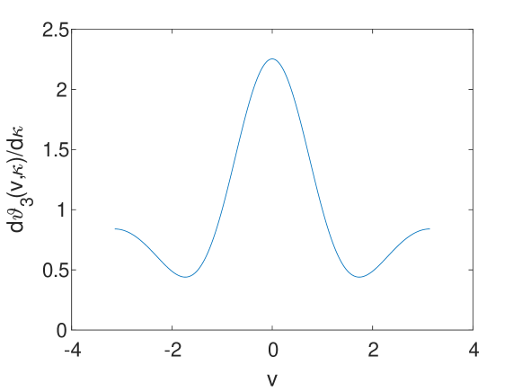
Figure 2: An example of derivation of the theta function with respect to $\kappa\pi$ for $\pi\kappa=0.5$: $\frac{d\,\vartheta_{3}(v,\kappa)}{d(\pi\kappa)}$, where $v=y/R=\phi$. Here we also use the definition of the theta function $\vartheta_{3}(v,\kappa)$ [15].

It should admitted that at the large time asymptotic, diffusion in fingers affects strongly anomalous diffusion in the backbone, and the former should be taken into account. Therefore, according to the Laplace inversion, the solution of Eq. (2.1) reads

$$P(x,y,t)=\frac{1}{\sqrt{2\pi R}}\sum_{k=0}^{\infty}\cos(ky/R){\cal L}^{-1}\left[f_{k}(s)e^{-|x|\sqrt{s/D_{2}}}\right]=\\ =\frac{1}{\sqrt{2\pi R}}\sum_{k=0}^{\infty}\cos(ky/R){\cal L}^{-1}\left[\frac{e^{-|x|\sqrt{s/D_{2}}}/\sqrt{D_{2}}}{2\left(\sqrt{s}+k^{2}D_{\frac{1}{2}}\right)}\right]=\\ =\frac{1}{2\pi\sqrt{2RD_{2}t}}e^{-\frac{x^{2}}{4D_{2}t}}+\bar{P}(x,y,t)\,,$$ (2.5)

where $D_{\frac{1}{2}}=\frac{D_{1}}{2\sqrt{D_{2}}}$. The term $\bar{P}(x,y,t)$ is estimated for the large time in B and reads

$$\bar{P}(x,y,t)=\frac{(2-\sqrt{\pi})}{4\pi\sqrt{2RD_{2}t}}e^{-\frac{x^{2}}{4D_{2}t}}\delta(y/R)+\frac{\pi^{3/2}|x|}{4D_{1}\sqrt{2D_{2}Rt^{3}}}B_{2}\left(\frac{y}{2\pi R}\right)e^{-\frac{x^{2}}{4D_{2}t}}\,,$$ (2.6)

where $B_{2}(z)$ is a shifted Bernoulli polynomial [16] defined on $z\in(-1/2,\,1/2)$, see Fig. 3.

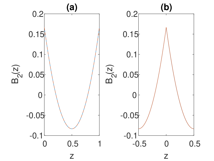
Figure 3: Bernoulli polynomial [16] $B_{2}(z)=z^{2}-z+1/6$ for $z\in[0,\,1]$ on panel (a), which is also the result of summation in Eq. (B.5). Another result of there is of the summation in Eq. (B.5) for $z\in[-1/2,\,1/2]$ is on panel (b). It consists of two parts for $z\in[0,\,1/2]$, which coincides with the left curve of $B_{2}(z)$. The second part for $z\in[-1/2,\,0]$ corresponds to the curve of the left part of $B_{2}(z)$ for $z\in[1/2,\,1]$ shifted on $1$.

In the polar coordinates the obtained result in Eqs. (2.5) and (2.6) reads

$$P(r,\phi,t)=\frac{1}{2\pi\sqrt{2RD_{2}t}}e^{-\frac{\ln^{2}(r/R)}{4D_{2}t}}\left[1+\frac{2-\sqrt{\pi}}{2}\delta(\phi)\right]+\\ +\frac{\pi^{3/2}|\ln(r/R)|}{4D_{1}\sqrt{2D_{2}Rt^{3}}}B_{2}\left(\frac{\phi}{2\pi}\right)e^{-\frac{\ln^{2}(r/R)}{4D_{2}t}}\,.$$ (2.7)

As obtained, the circular motion is not random due reflections on boundaries. It consists of two stationary distributions: the first one is the initial condition, which relaxes by power law as $t^{-1/2}$ and the second stationary distribution is according to the Bernoulli polynomial $B_{2}(\phi/2\pi)$, which interacts with the radial motion. The radial motion is random and corresponds to the geometric Brownian motion, which is described by the log-normal distribution [13], and leads to the exponential spreading along the radii with the mean squared displacement (MSD) $\langle r^{2}(t)\rangle\sim e^{t}$. This dominant process is also corrected by the Lévy-Smirnov distribution with respect to $\frac{t}{\ln(r/R)}$, see e.g., [17, 18]. Concluding this section it is worth to stress that the geometric Brownian motion is the geometry effect of the conformal mapping of the ($x-y$) comb model (2.1) onto the circular geometry comb by conformal gluing of the backbone ends.

3 Periodic boundary conditions

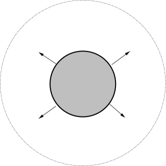
Figure 4: Schematic picture of the circular/umbrella comb with the periodic boundary conditions at $\phi=\pm\pi$ and outward diffusion along the radii with zero boundary conditions at infinity.

In the section, we consider the second scenario with periodic circular motion at $r=R$ and the outward radial motion with a constant diffusion coefficient $D_{r}=D$, see Fig. 4. Equation (1.1) now is

$$\partial_{t}P=D_{1}\delta(r-R)\frac{1}{r^{2}}\partial_{\phi}^{2}P+D\frac{1}{r}\partial_{r}r\partial_{r}P\,.$$ (3.1)

The initial condition is $P_{0}=P(r,\phi,t=0)=\delta(r-R)\delta(\phi)$ The distribution function $P=P(r,\phi,t)$ is a convolution integral

$$P(r,\phi,t)=\int_{0}^{t}G(r,t-t^{\prime})F(\phi,t^{\prime})dt^{\prime}\,,$$ (3.2)

which represents two independent motions in the Laplace space:

$$\tilde{P}(r,\phi,s)=g(r,s)f(\phi,s)\,.$$ (3.3)

This corresponds to Eq. (3.1) in the Laplace space,

$$s\tilde{P}-P_{0}=D_{1}\delta(r-R)\frac{1}{r^{2}}\partial_{\phi}^{2}\tilde{P}+D\frac{1}{r}\partial_{r}r\partial_{r}\tilde{P}\,.$$ (3.4)

Now, the boundary conditions for the radial motion can be easily specified for $\tilde{P}$, $g$ and $f$. These are $\tilde{P}(r=R,\phi,s)=f(\phi,s)$ and $g(r=R,s)=1$, and $\tilde{P}(r=\infty,\phi,s)=g(r=\infty,s)=\tilde{P}^{\prime}(r=\infty,\phi,s)=g^{\prime}(r=\infty,s)=0$, where prime means differentiation with respect to $r$. Note also, $f(\phi,s)$ is a multivalued function, and the conformal map cannot be performed. Therefore, we are treating the problem in the polar coordinates.

First, let us consider diffusion in radii - fingers. In the Laplace space, the diffusion equation from Eq. (3.4) leads to the equation

$$rsg=Drg^{\prime\prime}+Dg^{\prime}$$ (3.5)

with the solution

$$g(r,s)=A(s)K_{0}\left(r\sqrt{s/D}\right)\theta(r-R)\,,$$ (3.6)

where $K_{0}(z)$ is the modified Bessel function of the second kind, which satisfies the boundary conditions at infinity. The second boundary condition $g(R,s)=1$ yields $A(s)=2\left[K_{0}\left(R\sqrt{s/D}\right)\right]^{-1}$, where $\theta(0)=1/2$ is accounted.

Substituting solution (3.6) in Eq. (3.4), one obtains, see C

$$\partial_{\phi}^{2}f+af-bs^{\frac{1}{2}}f+c\delta(\phi)=0\,,$$ (3.7)

where $a=2RD/D_{1}$ and $bs^{1/2}=\frac{2R^{2}K_{1}(\lambda R)}{D_{1}K_{0}(\lambda R)}\sqrt{Ds}$, and $c=R^{2}/D_{1}$.

3.1 Initial time asymptotics

For the initial times, when $s\rightarrow\infty$, and $\lambda R=R\sqrt{s/D}\gg 1$, one obtains $\frac{K_{1}(\lambda R)}{K_{0}(\lambda R)}\approx 1$ and $a\ll bs^{\frac{1}{2}}$. Then, Eq. (3.7) is simplified with the solution

$$f(\phi,s)=\sum_{n=-\infty}^{\infty}\frac{ce^{in\phi}}{n^{2}+b\sqrt{s}}\,.$$ (3.8)

We also obtain that $g(r,s)\approx R^{\frac{1}{2}}e^{-\lambda(r-R)}/\sqrt{r}$ [16] and the PDF $P(r,\phi,t)$ leads to a chain of estimations in C. Therefore, the PDF reads

$$P(r,\phi,t)= {\cal L}^{-1}\left[g(r,s)f(\phi,s)\right]\approx\sum_{n=-\infty}^{\infty}\frac{cR^{\frac{1}{2}}}{br^{\frac{1}{2}}}e^{in\phi}\cdot{\cal L}^{-1}\left[\frac{e^{-\frac{\sqrt{s}(r-R)}{\sqrt{D}}}}{n^{2}/b+\sqrt{s}}\right]=$$ (3.9a)

$$= \frac{cR^{\frac{1}{2}}}{b\sqrt{r\pi t}}e^{-\frac{(r-R)^{2}}{4Dt}}[1+2\delta(\phi)]-\frac{2c(Dt/r)^{\frac{1}{2}}}{b(r-R)}e^{-\frac{(r-R)^{2}}{4Dt}}+$$ (3.9b)

$$+ \frac{c\pi\sqrt{RD^{\frac{1}{2}}}}{\sqrt{rb(r-R)}}\frac{\cosh\left[(\pi-|\phi|)\sqrt{D^{\frac{1}{2}}t/b(r-R)}\right]}{\cosh\left[\pi\sqrt{D^{\frac{1}{2}}t/b(r-R)}\right]}e^{-\frac{(r-R)^{2}}{4Dt}}\,,$$ (3.9c)

where $\phi\in[-\pi\,,\pi]$. The modulus $|phi|$ is due to the symmetry of Eq. (3.7). We also stress that the solution (3.9c) is valid for $r>R$, strictly. It should be noted that for $t\rightarrow 0$, the solution reduces to the transport for $r=R$, and Eq. (3.9a) reads

$$P(R,\phi,t)\approx\frac{c}{b\sqrt{\pi t}}[1+2\delta(\phi)]-\frac{2c}{\sqrt{t}}\sum_{n=1}^{\infty}\frac{\cos(n\phi)}{n^{2}}=\\ \frac{c}{b\sqrt{\pi t}}[1+2\delta(\phi)]-\frac{2c\pi^{2}}{\sqrt{t}}B_{2}\left(\frac{\phi}{2\pi}\right)\,.$$ (3.10)

The situation changes dramatically for the long times.

3.2 Large time asymptotics

For the large times, when $\lambda R\ll 1$, we have $K_{0}(\lambda R)\approx\ln\frac{2}{\gamma\lambda R}$ and $K_{1}(\lambda R)\approx 1/\lambda R$, where $\gamma$ is the Euler constant [16]. However, asymptotic behavior of $K_{0}(\lambda r)$ must correspond to the boundary conditions at $r\rightarrow\infty$. Therefore, we take the intermediate asymptotic, when $\lambda r>1$, which yields

$$K_{0}(\lambda R)\approx\sqrt{\frac{\pi}{2\lambda r}}e^{-\lambda r}=\sqrt{\pi(D/s)^{\frac{1}{2}}/r}e^{-r(s/D)^{\frac{1}{2}}}\,.$$

Correspondingly, in the limits $s\rightarrow 0$ and $rs^{\frac{1}{2}}D^{-\frac{1}{2}}>1$, the radial distribution $g(r,s)$ and the coefficient $b$ in Eq. (3.7) are functions of $s$ which are approximated as follows

$$g(r,s)\approx\sqrt{2\pi D^{\frac{1}{2}}/rs^{\frac{1}{2}}}\frac{e^{-r(s/D)^{\frac{1}{2}}}}{\ln\left(4D/\gamma^{2}R^{2}s\right)}\,,$$ (3.11a)

$$bs^{\frac{1}{2}}=b(s)s^{\frac{1}{2}}\approx\frac{4DR}{D_{1}}\ln^{-1}\left(4D/\gamma^{2}R^{2}s\right)\equiv b_{1}\left[\ln\left(4D/\gamma^{2}R^{2}s\right)\right]^{-1}\,.$$ (3.11b)

Again neglecting the parameter $a$ in Eq. (3.7), we obtain the solution as follows

$$f(\phi,s)=\sum_{n=-\infty}^{\infty}\frac{ce^{in\phi}\ln\left(D/\gamma^{2}R^{2}s\right)}{b_{1}+n^{2}\ln\left(D/\gamma^{2}R^{2}s\right)}\,.$$ (3.12)

Then the PDF (3.9) for the large time asymptotics reads in the form of the inverse Laplace transformation

$$P(r,\phi,t)={\cal L}^{-1}\left[g(r,s)f(\phi,s)\right]\approx\\ \approx{\cal L}^{-1}\left[\sum_{n=-\infty}^{\infty}\frac{2ce^{in\phi}}{n^{2}+b_{1}\ln\left(4D/\gamma^{2}R^{2}s\right)}\cdot\sqrt{2\pi(D/r^{2}s)^{\frac{1}{2}}}e^{-r(s/D)^{\frac{1}{2}}}\right]\,.$$ (3.13)

The solution, obtained in C, reads

$$P(r,\phi,t)\approx\frac{c\pi}{b_{1}\Gamma\left(\frac{1}{4}\right)}\frac{\sqrt{2\pi(D/t^{3}r^{2})^{\frac{1}{2}}}}{\ln^{\frac{1}{2}}\left(4Dt/\gamma^{2}R^{2}\right)}e^{-3r^{2}/8Dt}\\ \times\Biggl{\{}\frac{\ln^{-\frac{1}{2}}\left(4Dt/\gamma^{2}R^{2}\right)}{\pi}+\frac{\cosh\left[(\pi-|\phi|)\sqrt{b_{1}\ln\left(4Dt/\gamma^{2}R^{2}\right)}\right]}{\cosh\left[\pi\sqrt{b_{1}\ln\left(4Dt/\gamma^{2}R^{2}\right)}\right]}\Biggr{\}}\,.$$ (3.14)

This result is valid for $r\gg R$ and $t\rightarrow\infty$, and the Tauberian theorem, applied in Eq. (C.12), grasps exactly this intermediate asymptotic behavior of $K_{0}(\lambda r)\propto r^{-\frac{1}{2}}s^{-\frac{1}{4}}$ due to the power law. The logarithmic evolution in the backbone shown in Fig. 5, relaxes to the radii-fingers. However, in large time asymptotic calculation this backbone relaxation cannot be separated from the radii one. Note also that the approximate solution (3.14) for the PDF in the specific area does not conserve the probability ${\cal P}$, namely the latter is

$${\cal P}(t)=\int_{0}^{\infty}dr\int_{-\pi}^{\pi}d\phi P(r,\phi,t)\sim t^{-\frac{1}{2}}\,.$$ (3.15)

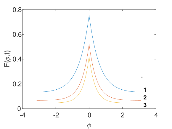
Figure 5: Evolution of the braces $F(\phi,t)$ in PDF of Eq. (3.14). The plots are dependence of $F(\phi,t)$ on $\phi$ for three times where plot 1 corresponds to $t=10$, 2 to $t=100$ and 3 to $t=1000$. All parameters are taken to be one, while $\gamma=1.781$

3.3 The MSD in radii

This also results to radii subdiffusion with the mean squared displacement (MSD) of the order of $\langle r^{2}(t)\rangle\sim Dt$. Indeed, the relaxation process in the backbone contributes to the transport in fingers with the MSD defined from the inverse Laplace transformation in Eq. (3.13) as follows

$$\langle r^{2}(t)\rangle={\cal P}^{-1}(t){\cal P}^{-1}(t)\frac{1}{2\pi}\int_{R}^{\infty}\int_{-\pi}^{\pi}r^{2}P(r,\phi,t)drd\phi=\\ ={\cal L}^{-1}\left[\frac{2c}{b_{1}\ln\left(4D/\gamma^{2}R^{2}s\right)}\cdot\sqrt{2\pi(D/s)^{\frac{1}{2}}}\int_{R}^{\infty}r^{3/2}e^{-r(s/D)^{\frac{1}{2}}}dr\right]\propto\\ \propto D{\cal P}^{-1}(t){\cal L}^{-1}\Big{[}s^{-3/2}\Gamma\left(\frac{3}{2},R\sqrt{s}\right)\Big{]}(t)\,,$$ (3.16)

where $\Gamma(\alpha,z)$ is the incomplete gamma function [16] and the factor ${\cal P}^{-1}(t)$ is due to the non conserved probability. Performing the Laplace inversion by means of the Tauberian theorem, see C, we obtain a subdiffusive growth of the order of $Dt^{1/2}$ However, the obtained expression should be normalized by the probability ${\cal P}(t)$. This eventually yields the MSD in the form of normal diffusion

$$\langle r^{2}(t)\rangle\sim Dt\,.$$

4 Conclusion

A circular comb is considered, and two scenarios of the anomalous transport in the circular comb geometry are studied. The first scenario corresponds to the conformal mapping of a comb Fokker-Planck equation on the umbrella comb. In this case, the reflecting boundary conditions are imposed on the circular (rotator) motion, while the radial motion corresponds to geometric Brownian motion with vanishing to zero boundary conditions on infinity. The radial diffusion is described by the log-normal distribution, which corresponds to exponentially fast motion with the MSD of the order of $e^{t}$. The second scenario corresponds to circular diffusion with periodic boundary conditions and the outward Brownian radial diffusion with vanishing to zero boundary conditions at infinity. In this case the radial motion is normal diffusion with the MSD of the order of $t$. However the circular motion in both scenarios is a superposition of cosine functions that results in a stationary distribution in the form of the Bernoulli polynomials, with the power law relaxation.

Appendix A Backbone dynamics with RBC

Note that “RBC” means reflecting boundary conditions at $y=\pm\pi R$.

Let us consider Eq. (2.2b)

$$D_{1}\partial_{y}^{2}f(y,s)-2\sqrt{sD_{2}}f(y,s)+\delta(y/R)=0\,,$$ (A.1)

which describes anomalous diffusion, namely subdiffusion, along the $y$-axis-backbone. Recall that it also corresponds to anomalous diffusion in the ring backbone of the umbrella comb. Due to the reflection boundary conditions $f^{\prime}(y=\pm\pi R,s)=0$, the solution can be presented as the superposition of the even eigenfunctions $\frac{1}{\sqrt{2\pi R}}\cos(ny/R)$. It reads

$$f(y,s)=\frac{1}{\sqrt{2\pi R}}\sum_{n=0}^{\infty}f_{n}(s)\cos(ny/R)\,.$$ (A.2)

From Eq. (A.1), this yields

$$f_{n}(s)=\frac{1}{2\sqrt{2\pi RD_{2}}}\frac{1}{\sqrt{s}+D_{\frac{1}{2}}n^{2}}\,,$$ (A.3)

where $D_{\frac{1}{2}}=D_{1}/2\sqrt{D_{2}}$ is a subdiffusion coefficient. Performing the inverse Laplace transform, one obtains the solution in the form of the Mittag-Leffler function [15]

$$f_{n}(t)=\frac{1}{2\sqrt{2\pi RD_{2}}}\frac{1}{2\pi i}\int_{-i\infty}^{i\infty}\frac{e^{st}}{\sqrt{s}+D_{\frac{1}{2}}n^{2}}ds=\\ =\frac{t^{-1/2}}{2\sqrt{2\pi RD_{2}}}E_{\frac{1}{2},\frac{1}{2}}\left(-n^{2}D_{\frac{1}{2}}t^{\frac{1}{2}}\right)\,.$$ (A.4)

Using properties of the Mittag-Leffler functions [15]

$$E_{\alpha,1}(z)=E_{\alpha}(z)\quad\text{and}\quad E_{\alpha,\beta}(z)=\frac{1}{\Gamma(\beta)}+zE_{\alpha,\alpha+\beta}(z)\,,$$

$$E_{\alpha,\beta}(z)=\sum_{k=0}^{\infty}\frac{z^{k}}{\Gamma(k\alpha+\beta)}\,,$$

where $\Gamma(\nu+1)=\nu\Gamma(\nu)$ is a gamma function, we obtain the initial behavior of $f_{n}(t)$ in Eq. (A.4):

$$f_{n}(t)=\frac{1}{2\sqrt{2\pi RD_{2}}}\left[\frac{t^{-1/2}}{\Gamma(1/2)}-n^{2}D_{\frac{1}{2}}E_{\frac{1}{2}}\left(-n^{2}D_{\frac{1}{2}}t^{\frac{1}{2}}\right)\right]=\\ =\frac{1}{2\sqrt{2\pi RD_{2}}}\left\{\frac{t^{-1/2}}{\Gamma(1/2)}-n^{2}D_{\frac{1}{2}}\cdot\exp\left[-n^{2}D_{\frac{1}{2}}t^{\frac{1}{2}}/\Gamma(3/2)\right]\right\}\,,$$ (A.5)

where $\Gamma(1/2)=\sqrt{\pi}$. Taking into account the expansion (A.2), we obtain the first term in Eq. (A.5) in the form of the pining initial condition decaying with time, while the second term is the theta function $\vartheta_{3}(y/R,\kappa)$. Then Eq. (A.2) reads

$$f(y,t)=P(x=0,y,t)=\frac{t^{-1/2}}{4\pi R\sqrt{\pi D_{2}}}\sum_{n=0}^{\infty}\cos(ny/R)-\\ -\frac{t^{-1/2}D_{\frac{1}{2}}}{4\pi R\sqrt{\pi D_{2}}}\sum_{n=1}^{\infty}\cos(ny/R)n^{2}e^{-\kappa\pi n^{2}}=\\ =\frac{t^{-1/2}}{4\pi R\sqrt{\pi D_{2}}}(\delta(y/R)+1)+\frac{t^{-1/2}D_{\frac{1}{2}}}{4\pi^{2}R\sqrt{\pi D_{2}}}\frac{d}{d\kappa}\vartheta_{3}(y/R,\kappa)\,,$$ (A.6)

where $\kappa=2D_{\frac{1}{2}}t^{\frac{1}{2}}/\pi^{3/2}$. Here we also use the definition of the theta function $\vartheta_{3}(y/R,\kappa)$ [15]. A typical behavior of $\frac{d}{d\kappa}\vartheta_{3}(y/R,\kappa)$ for $\pi\kappa=0.5$ is shown in Fig. 2.

Appendix B Long time asymptotic

The long time diffusion can be estimated from Eq. (A.4), as well. To that end we take into account that the Laplace inversion of the Mittag-Leffler function can be presented in the form of the error function $\mathrm{Erfc}(z)$ [19], as follows

$$E_{\frac{1}{2},\frac{1}{2}}(at^{\frac{1}{2}})=\frac{1}{\sqrt{\pi t}}-ae^{a^{2}t}\mathrm{Erfc}\left(at^{\frac{1}{2}}\right)\,.$$ (B.1)

However, at the large time asymptotics, diffusion in fingers affects strongly anomalous diffusion in the backbone, and the former should be taken into account. Therefore, we consider the inverse Laplace transformation in Eq. (2.5), which is the table integral [19] of the form

$$\sum_{n=0}^{\infty}\cos(ny/R){\cal L}^{-1}\left[\frac{e^{-a\sqrt{s}}}{\sqrt{s}+b}\right]=(\pi t)^{-1/2}e^{-a^{2}(4t)^{-1}}-\sum_{n=1}^{\infty}\cos(ny/R)\\ \times\left[(\pi t)^{-1/2}e^{-a^{2}(4t)^{-1}}-be^{ba+b^{2}t}\mathrm{Erfc}\left(2^{-1}at^{-1/2}+bt^{1/2}\right)\right]\,.$$ (B.2)

Here parameters $a$ and $b$ are determined from Eqs. (2.5) and (A.4). Namely, $a=|x|/\sqrt{D_{2}}$ determines radial diffusion, while $b=D_{\frac{1}{2}}n^{2}$ specifies backbone subdiffusion as obtained above. The error function in Eq. (B.2) for the large argument reads

$$\mathrm{Erfc}\left(2^{-1}at^{-1/2}+bt^{1/2}\right)\approx\frac{e^{-\frac{a^{2}}{4t}-ab-b^{2}t}}{at^{-1/2}+2bt^{1/2}}\approx\\ \approx e^{-\frac{a^{2}}{4t}-ab-b^{2}t}\left[(2b)^{-1}t^{-1/2}-a(2b)^{-2}t^{-3/2}\right]\,.$$ (B.3)

Taking into account expansion (A.2) and Eqs. (2.5), (B.2), and (B.3), and values of $a$ and $b$, we obtain

$$P(x,y,t)=\frac{1}{2\sqrt{2\pi D_{2}R}}\sum_{n=0}^{\infty}\cos(ny/R){\cal L}^{-1}\left[\frac{e^{-a\sqrt{s}}}{\sqrt{s}+b}\right]=\\ =\frac{1}{2\pi\sqrt{2D_{2}t}}e^{\frac{x^{2}}{4D_{2}t}}+\bar{P}(x,y,t)=\\ =\frac{1}{2\pi\sqrt{2RD_{2}t}}e^{-\frac{x^{2}}{4D_{2}t}}\left[1+\delta(y/R)\right]-\frac{1}{4\sqrt{2\pi RD_{2}t}}e^{-\frac{x^{2}}{4D_{2}t}}\delta(y/R)\\ +\frac{|x|}{4D_{1}\sqrt{2\pi D_{2}Rt^{3}}}e^{-\frac{x^{2}}{4D_{2}t}}\sum_{n=1}^{\infty}\frac{\cos(ny/R)}{n^{2}}\,.$$ (B.4)

Estimating the last term in Eq. (B.4), which is [20]

$$\sum_{n=1}^{\infty}\frac{\cos(ny/R)}{n^{2}}=\pi^{2}B_{2}\left(\frac{y}{2\pi R}\right)\,,$$ (B.5)

we obtain

$$\bar{P}(x,y,t)=\frac{(2-\sqrt{\pi})}{4\pi\sqrt{2RD_{2}t}}e^{-\frac{x^{2}}{4D_{2}t}}\delta(y/R)+\frac{\pi^{3/2}|x|}{4D_{1}\sqrt{2D_{2}Rt^{3}}}B_{2}\left(\frac{y}{2\pi R}\right)e^{-\frac{x^{2}}{4D_{2}t}}\,.$$ (B.6)

Here $B_{2}(z)$ is a shifted Bernoulli polynomial presented on $z\in(-1/2,\,1/2)$, see Fig. 3. It should be admitted that for the standard definition of the Bernoulli polynomial, $B_{2}(z)=z^{2}-2z+1/6$ is defined on $z\in(0,1)$ [16]

Appendix C Backbone dynamic with PBC

Note that “PBC” means periodic boundary conditions at $\phi=\pm\pi$.

Let us consider the radial motion in Eq. (3.4) according to the radial derivative $\frac{1}{r}\partial_{r}r\partial_{r}g=g^{{}^{\prime\prime}}+r^{-1}g^{\prime}$, where $g=g(r,s)$ is the solution of Eq. (3.5)

$$g(r,s)=\frac{2K_{0}\left(\lambda r\right)}{K_{0}\left(\lambda R\right)}\theta(r-R)\,,\quad\lambda=\sqrt{s/D}\,$$ (C.1)

in the form is the modified Bessel function of the second kind $K_{0}(z)$, which satisfies the boundary conditions at infinity. Using properties of its derivatives [16] as follows

$$K_{0}^{\prime}(z) =-K_{1}(z)\,,$$ (C.2a)

$$K_{0}^{\prime\prime}(z) =-K_{1}^{\prime}(z)=\frac{1}{2}\left[K_{0}(z)+K_{2}(z)\right]\,,$$ (C.2b)

$$-K_{1}^{\prime}(z) =K_{0}(z)+\frac{1}{z}K_{1}(z)\,,$$ (C.2c)

we have

$$g^{\prime}(r,s)=\frac{2}{K_{0}(\lambda R)}\left[-\lambda K_{1}(\lambda r)\theta(r-R)+K_{0}(\lambda r)\delta(r-R)\right]$$ (C.3)

and

$$g^{\prime\prime}(r,s)=\frac{2}{K_{0}(\lambda R)}\left[\lambda^{2}K_{0}(\lambda r)\theta(r-R)+\right.\\ \left.+\lambda r^{-1}K_{1}(\lambda r)\theta(r-R)-\lambda K_{1}(\lambda r)\delta(r-R)\right]\,,$$ (C.4)

where $-K_{0}(\lambda r)\delta^{\prime}(r-R)=\lambda K_{1}(\lambda r)\delta(r-R)$ is used. Therefore, the superposition of Eqs. (C.3) and (C.4) yields

$$g^{\prime\prime}(r,s)+\frac{1}{r}g^{\prime}(r,s)=\frac{2}{K_{0}(\lambda R)}\left[\lambda^{2}K_{0}(\lambda r)\theta(r-R)+\right.\\ \left.+\frac{1}{R}K_{0}(\lambda r)\delta(r-R)-\lambda K_{1}(\lambda r)\delta(r-R)\right]\,.$$ (C.5)

Inserting the obtained result (C.5) in Eq. (3.4) and taking into account Eq. (3.3), we obtain the equation for $f(\phi,s)$ as follows

$$D_{1}\frac{1}{R^{2}}\partial_{\phi}^{2}f+\left[\frac{2D}{R}-\frac{2K_{1}(\lambda R)}{K_{0}(\lambda R)}\sqrt{Ds}\right]f+\delta(\phi)=0\,.$$ (C.6)

C.1 Initial time asymptotics

For the initial times, when $s\rightarrow\infty$, and $\lambda R=R\sqrt{s/D}\gg 1$, it is obtained that $f(\phi,s)$ is determined by Eq. (3.8). Taking into account the solution (3.8) and accounting that $g(r,s)\approx R^{\frac{1}{2}}e^{-\lambda(r-R)}/\sqrt{r}$ [16], we obtain for the PDF $P(r,\phi,t)$ the following chain of estimations (see also B)

$$P(r,\phi,t)={\cal L}^{-1}\left[g(r,s)f(\phi,s)\right]\approx{\cal L}^{-1}\left[\sum_{n=-\infty}^{\infty}\frac{cR^{\frac{1}{2}}}{br^{\frac{1}{2}}}e^{in\phi}\cdot\frac{e^{-\frac{\sqrt{s}(r-R)}{\sqrt{D}}}}{n^{2}/b+\sqrt{s}}\right]\,.$$ (C.7)

Performing the Laplace inversion, separating term with $n=0$, and accounting Eqs. (B.2), (B.3), we obtain

$$P(r,\phi,t)=\frac{cR^{\frac{1}{2}}}{br^{\frac{1}{2}}\sqrt{\pi t}}e^{-\frac{(r-R)^{2}}{4Dt}}[1+2\delta(\phi)]-\sum_{n=1}^{\infty}\frac{2cR}{br}\cos(n\phi)\\ \times e^{n^{2}(r-R)b^{-1}D^{-\frac{1}{2}}+b^{-2}n^{4}t}\mathrm{Erfc}\left(2^{-1}(r-R)D^{-\frac{1}{2}}t^{-1/2}+n^{2}b^{-1}t^{1/2}\right)\approx\\ \approx\frac{cR^{\frac{1}{2}}}{b\sqrt{\pi rt}}e^{-\frac{(r-R)^{2}}{4Dt}}[1+2\delta(\phi)]-\frac{2cR^{\frac{1}{2}}}{\sqrt{rt}}\sum_{n=1}^{\infty}\frac{\cos(n\phi)e^{-\frac{(r-R)^{2}}{4Dt}}}{2^{-1}b(r-R)D^{-\frac{1}{2}}t^{-1}+n^{2}}=\\ =\frac{cR^{\frac{1}{2}}}{b\sqrt{r\pi t}}e^{-\frac{(r-R)^{2}}{4Dt}}[1+2\delta(\phi)]-\frac{2c(RDt/r)^{\frac{1}{2}}}{b(r-R)}e^{-\frac{(r-R)^{2}}{4Dt}}+\\ +\frac{c\pi\sqrt{RD^{\frac{1}{2}}}}{\sqrt{rb(r-R)}}\frac{\cosh\left[(\pi-|\phi|)\sqrt{D^{\frac{1}{2}}t/b(r-R)}\right]}{\cosh\left[\pi\sqrt{D^{\frac{1}{2}}t/b(r-R)}\right]}e^{-\frac{(r-R)^{2}}{4Dt}}\,,$$ (C.8)

where $\phi\in[-\pi\,,\pi]$. Note, that the modulus $|phi|$ is due to the symmetry of Eq. (3.7). We also stress that the solution is valid for $r>R$, strictly. For $r=R$, Eq. (C.8) reads

$$P(r,\phi,t)\approx\frac{c}{b\sqrt{\pi t}}[1+2\delta(\phi)]-\frac{2c}{\sqrt{t}}\sum_{n=1}^{\infty}\frac{\cos(n\phi)}{n^{2}}=\\ =\frac{c}{b\sqrt{\pi t}}[1+2\delta(\phi)]-\frac{2c\pi^{2}}{\sqrt{t}}B_{2}\left(\frac{\phi}{2\pi}\right)\,.$$ (C.9)

C.2 Large time asymptotics

In this section we estimate Eq. (3.13). Performing the inverse Laplace transformation in Eq. (3.13), we have

$$P(r,\phi,t)={\cal L}^{-1}\left[g(r,s)f(\phi,s)\right]\approx\\ \approx{\cal L}^{-1}\left[\sum_{n=-\infty}^{\infty}\frac{2ce^{in\phi}}{n^{2}+b_{1}\ln\left(4D/\gamma^{2}R^{2}s\right)}\cdot\sqrt{2\pi(D/r^{2}s)^{\frac{1}{2}}}e^{-r(s/D)^{\frac{1}{2}}}\right]\,.$$ (C.10)

Performing the Laplace inversion term by term in the summation $\sum_{n}A_{n}(s)$, we have

$${\cal L}^{-1}\left[A_{n}(s)\right](t)={\cal L}^{-1}\left[\frac{d_{1}s^{-1/4}}{n^{2}+S(s)}e^{-d_{2}\sqrt{s}}\right]\,,$$ (C.11)

where $S(s)=b_{1}\ln\left(4D/\gamma^{2}R^{2}s\right)$ and $e^{-d_{2}\sqrt{s}}\sim\left(1+d_{2}s^{\frac{1}{2}}\right)^{-1}$. Making scaling by $\lambda$, we obtain from Eq. (C.11) that $A_{n}(\lambda s)/A_{n}(s)\sim\lambda^{-1/4}$ for $s\rightarrow 0$, while $[n^{2}+S(s)]^{-1}$ is slow functions of $1/s$. Therefore, $A_{n}(s)=s^{-\rho}e^{-d_{2}\sqrt{s}}L(1/s)$, where $L(1/s)=[n^{2}+S(s)]^{-1}$ is a slow function of $1/s$ and $\rho=1/4$. Then applying the Tauberian theorem, we obtain [21] $A_{n}(t)=t^{\rho-1}e^{-3d_{2}^{2}/8t}L(t)/\Gamma(\rho)$, see Sec. C.3 below. Expression (C.10) reads now as follows

$$P(r,\phi,t)\approx\sqrt{2\pi(D/t^{3}r^{2})^{\frac{1}{2}}}e^{-3r^{2}/8Dt}\sum_{n=-\infty}^{\infty}\frac{2ce^{in\phi}}{\Gamma(1/4)[n^{2}+S(t)]}\,,$$ (C.12)

where $S(t)=b_{1}\ln\left(4Dt/\gamma^{2}R^{2}\right)$. The summation yields [20]

$$\sum_{n=-\infty}^{\infty}\frac{2ce^{in\phi}}{n^{2}+S(t)}=\frac{2c}{S(t)}+\sum_{n=1}^{\infty}\frac{2c\cos(n\phi)}{n^{2}+S(t)}=\\ =\frac{2c}{S(t)}+\frac{c\pi}{\sqrt{S(t)}}\cdot\frac{\cosh\left[(\pi-|\phi|)\sqrt{S(t)}\right]}{\cosh\left[\pi\sqrt{S(t)}\right]}-\frac{c}{S(t)}\,.$$ (C.13)

Eventually, one obtains the PDF for the large time asymptotics as follows

$$P(r,\phi,t)\approx\frac{c\pi}{b_{1}\Gamma\left(\frac{1}{4}\right)}\cdot\frac{\sqrt{2\pi(D/t^{3}r^{2})^{\frac{1}{2}}}}{\ln^{\frac{1}{2}}\left(4Dt/\gamma^{2}R^{2}\right)}e^{-3r^{2}/8Dt}\\ \times\Biggl{\{}\frac{\ln^{-\frac{1}{2}}\left(4Dt/\gamma^{2}R^{2}\right)}{\pi}+\frac{\cosh\left[(\pi-|\phi|)\sqrt{b_{1}\ln\left(4Dt/\gamma^{2}R^{2}\right)}\right]}{\cosh\left[\pi\sqrt{b_{1}\ln\left(4Dt/\gamma^{2}R^{2}\right)}\right]}\Biggr{\}}\,.$$ (C.14)

C.3 The Tauberian theorem

Let us consider the Laplace inversion of $A_{n}(s)=s^{-\rho}e^{-d_{2}\sqrt{s}}$ with $\rho=1/4$. To this end let us consider the exponential in the form of the Fourier transform

$$\int_{-\infty}^{\infty}\frac{e^{ikd_{2}}dk}{(k+is^{\frac{1}{2}})(k-is^{\frac{1}{2}})}=\frac{\pi e^{-d_{2}\sqrt{s}}}{\sqrt{s}}\,,\quad d_{2}>0\,.$$ (C.15)

Since the PDF is a real function, thus we take the real part of the integrations to avoid artificial complex parts that can appear due to this trick. Therefore, we have the

$$A_{n}(t)=\mathrm{Re}{\cal L}^{-1}[A_{n}(s)](t)=\frac{1}{2\pi^{2}i}\int_{-\infty}^{\infty}e^{ikd_{2}}\int_{C}\frac{s^{\frac{1}{4}}e^{st}}{s+k^{2}}dsdk=\\ =\mathrm{Re}\frac{t^{-\frac{1}{4}}}{\pi}\int_{-\infty}^{\infty}e^{-k^{2}t+ikd_{2}}k^{\frac{1}{2}}dk=\frac{t^{-\frac{3}{4}}}{\pi}\int_{0}^{\infty}e^{-z^{2}+izkd_{2}}z^{\frac{1}{2}}dz=\\ =\frac{(4t)^{-\frac{3}{4}}}{\pi}\Gamma(\frac{3}{2})\Psi\left(\frac{3}{4},\frac{1}{2};-\frac{d_{2}^{2}}{4t}\right)\approx\\ \approx\frac{(4t)^{-\frac{3}{4}}}{\pi}\frac{\Gamma(\frac{3}{2})\Gamma(\frac{1}{2})}{\Gamma(\frac{5}{4})}\left(1-\frac{3d_{2}^{2}}{8t}\right)\propto t^{-\frac{3}{4}}e^{-\frac{3d_{2}^{2}}{8t}}\,.$$ (C.16)

Here $\Psi(a,s;z)$ is the degenerate hypergeometric function, obtained in the second integration with respect to $z$, which is a table integral [20].

References

References

- [1] Y. Fan, L. Liu, L. Zheng, X. Li, Subdiffusions on circular branching structures, Commun. Nonlinear Sci. Numer. Simulat. 77: 225 - 238, 2019.
- [2] Ch. Liu, Y. Fan, P. Lin, Numerical investigation of a fractional diffusion model on circular comb-inward structure, Appl. Math. Lett. 100: 106053, 2020.
- [3] A. V. Milovanov and J. J. Rasmussen, Lévy flights on a comb and the plasma staircase, Phys. Rev E 98: 022208, 2018.
- [4] D. S. Grebenkov Analytical solution for restricted diffusion in circular and spherical layers under inhomogeneous magnetic fields, J. Chem. Phys. 128: 134702, 2008.
- [5] A. J. Lichtenberg and M. A. Lieberman, Regular and Stochastic Motion, Springer, New York, 1983.
- [6] A. Iomin, Chaotic overlap of cyclotron resonances in the Azbel’ - Kaner effect, Phys. Rev. B 49: R4341 - R4343, 1994.
- [7] A. Iomin, Quantum localization of chaos in a ring, Phys. Rev. E 52: R5743 - R5745, 1995.
- [8] M. A. Lavrentyev and B.V. Shabat, Methods of the theory of functions of complex variable, Nauka, Moscow, 1987.
- [9] R. K. Bhaduri, A. Khare, and J. Law, Phase of the Riemann zeta function and the inverted harmonic oscillator, Phys. Rev. E 52: 486 - 491, 1995.
- [10] S. Nonnenmacher and A. Voros, Eigenstate structures around a hyperbolic point, J. Phys. A 30: 295 - 315, 1997.
- [11] G. P. Berman and M. Vishik, Long time evolution of quantum averages near stationary points, Phys. Lett. A 319: 352 - 359, 2003.
- [12] A. Iomin, Exponential spreading and singular behavior of quantum dynamics near hyperbolic points, Phys. Rev. E 87: 054901, 2013.
- [13] S. M. Ross, Introduction to Probability Models, Academic Press, London, 2019.
- [14] F. Black and M. Scholes, The pricing of options and corporate liabilities, J. Polit. Econ. 81: 637 - 654, 1973.
- [15] H. Bateman and A. Erdélyi, Higher Transcendental Functions, [V. 3], McGraw-Hill, New York, 1955.
- [16] M. Abramovitz and I. A. Stegun, Handbook of Mathematical Functions with Formulas, Graphs, and Mathematical Tables, Dover Publications, New York, 1972.
- [17] V. Uchaikin and R. Sibatov, Fractional Kinetics in Solids, World Scientific, Singapore, 2013.
- [18] V. Méndez, S. Fedotov, and W. Horsthemke, Reaction–Transport Systems, Springer, New York, 2010
- [19] H. Bateman and A. Erdélyi, Tables of Integral Transforms, [V. 1], McGraw-Hill, New York, 1954.
- [20] A. P. Prudnikov, Yu. A. Brychkov, and O. I. Marichev, Integrals and series, [V. 1], Gordon and Breach, New York, 1986.
- [21] W. Feller, An Introduction to Probability Theory and its Applications, [V. 2], Wiley, New York, 1971.