Sequential Linearization Method for Bound-Constrained Mathematical Programs with Complementarity Constraints

Abstract

We propose an algorithm for solving bound-constrained mathematical programs with complementarity constraints on the variables. Each iteration of the algorithm involves solving a linear program with complementarity constraints in order to obtain an estimate of the active set. The algorithm enforces descent on the objective function to promote global convergence to B-stationary points. We provide a convergence analysis and preliminary numerical results on a range of test problems. We also study the effect of fixing the active constraints in a bound-constrained quadratic program that can be solved on each iteration in order to obtain fast convergence.

1 Introduction

We consider the bound-constrained mathematical program with complementarity constraints (MPCC) of the form

$$\begin{aligned} \mathop{\rm minimize}_{x}\ &f(x)\\ \textnormal{subject\ to:}\ &\ell_{0}\leq x_{0}\leq u_{0},\\ &0\leq x_{1}\;\perp\;x_{2}\geq 0,\end{aligned}$$ (1)

where $f$ is smooth and $x\coloneqq(x_{0},x_{1},x_{2})\in\mathbb{R}^{n}$ is a partition of the variables into bound-constrained variables $x_{0}$ (e.g., controls) and complementarity variables $x_{1}$, $x_{2}$ (e.g., states). We let $n\coloneqq n_{0}+2n_{1}$, with $x_{0}\in\mathbb{R}^{n_{0}}$ and $x_{1}$, $x_{2}\in\mathbb{R}^{n_{1}}$, where $n_{0}$, $n_{1}$ are nonnegative integers. We let $\ell_{0,i}$ denote element $i$ of $\ell_{0}$ and similarly for $u_{0}$, $x_{0}$, $x_{1}$, and $x_{2}$ as well. We also assume that, without loss of generality, $\ell_{0,i}<u_{0,i}$ for $i\in\{1,\ldots,n_{0}\}$, because otherwise we could remove variable $x_{0,i}$ by fixing it to be $\ell_{0,i}=u_{0,i}=x_{0,i}$. The feasible set of (1) is nonempty because $\ell_{0}<u_{0}$.

Motivation

Problems of the form (1) appear as subproblems in an augmented Lagrangian approach for solving more general MPCCs. This approach extends existing augmented Lagrangian approaches for standard nonlinear programs such as [4, 21, 11], LANCELOT [8, 9], or TANGO, [2, 3] to MPCCs. To see how (1) can appear as a subproblem, consider the general MPCC

$$\mathop{\rm minimize}_{x} f(x)$$ (2)

subject to: $$c(x)=0,$$

$$0\leq g(x)\;\perp\;h(x)\geq 0,$$

where $c:\mathbb{R}^{n}\to\mathbb{R}^{m}$, and $g,h:\mathbb{R}^{n}\to\mathbb{R}^{p}$, are smooth functions for some $m,p\in\mathbb{N}$. By introducing slack variables $s_{g},s_{h}\in\mathbb{R}^{p}$, (2) can be written as a problem with simple complementarity constraints:

$$\mathop{\rm minimize}_{x,s_{g},s_{h}} f(x)$$

subject to: $$c(x)=0,\;s_{g}-g(x)=0,\;s_{h}-h(x)=0,$$

$$0\leq s_{g}\;\perp\;s_{h}\geq 0.$$

By introducing Lagrange multipliers $y,z_{g},z_{h}$ for the three sets of equality constraints, we obtain an augmented Lagrangian of (2)

$${\cal L}_{\rho}(x,s_{g},s_{h},y,z_{g},z_{h})\coloneqq f(x)-y^{T}c(x)-z_{g}^{T}(s_{g}-g(x))-z_{h}^{T}(s_{h}-h(x))$$

$$+\frac{\rho}{2}\left(\|c(x)\|_{2}^{2}+\|s_{g}-g(x)\|_{2}^{2}+\|s_{h}-h(x)\|_{2}^{2}\right),$$

and the augmented Lagrangian subproblem associated with (2) becomes

$$\begin{aligned} \mathop{\rm minimize}_{x,s_{g},s_{h}}\ &{\cal L}_{\rho}(x,s_{g},s_{h},y,z_{g},z_{h})\\ \textnormal{subject\ to:}\ &0\leq s_{g}\;\perp\;s_{h}\geq 0,\end{aligned}$$ (3)

which has the same structure as (1).

Related Work

We propose to solve (1) with a trust-region strategy that respects the complementarity constraints in every iteration. Because all iterates are feasible for (1), every accepted step also provides an estimate of the active set. While we are not aware of any publication that analyzes this described setting and method, active set and trust-region methods have been used for MPCCs in the past. Scholtes and Stöhr [35] analyze a trust-region method on exact penalty functions that arise from MPCCs. Fukushima and Tseng [22] iteratively compute approximate KKT-points of nonlinear programs (NLPs) that arise from $\varepsilon$-active sets induced by the previous iterates, where $\varepsilon$ is a slack parameter that is driven to zero over the iterations. Júdice et al. [25] and Chen and Goldfarb [6] propose active set strategies that also respect the complementarity constraints in every iteration by alternatingly computing descent steps (projected Newton steps in [6]) on the null space of the active constraints and updating entries of the active set based on the Lagrange multipliers.

Notation

We use subscripts to identify components of vectors or matrices, and superscripts to indicate iterates. Similarly, functions that are evaluated at particular points are denoted as $f^{k}\coloneqq f(z^{k})$, for example.

Structure of the Remainder

We present our algorithm to solve (1) in Section 2. Then its execution is demonstrated on an example problem in Section 3. Section 4 analyzes the convergence of the iterates. Section 5 presents two approaches for including second-order information into the algorithm in order to improve its convergence speed. In Section 6, we present computational results for two sets of benchmark problems. We show in Section 7 that our developments generalize to lower and upper bounds on $x_{1},x_{2}$, and mixed complementarity conditions between $x_{1}$ and $x_{2}$.

2 Algorithm Statement

We now introduce our SLPCC algorithm that solves a sequence of linear programs with complementarity constraints. We will show that it converges to B-stationary (or Bouligand stationary) points.

Definition 2.1 ([29], §3.3.1).

A feasible point $x^{*}$ of (1) is called B-stationary if $d=0$ is a local minimizer of the linear program with complementarity constraints (LPCC) obtained by linearizing $f$, about $x^{*}$:

$$\mathop{\rm minimize}_{d} \nabla f(x^{*})^{T}d$$ (1)

subject to: $$\ell_{0}\leq x_{0}^{*}+d_{0}\leq u_{0}$$

$$0\leq x_{1}^{*}+d_{1}\;\perp\;x_{2}^{*}+d_{2}\geq 0,$$

where the step $d$ is partitioned as $d\coloneqq\begin{pmatrix}d_{0},d_{1},d_{2}\end{pmatrix}$.

The B-stationarity condition in Definition 2.1 is also referred to as linearized B-stationarity [15], although it is easy to see that the two definitions are equivalent because of the simple structure of the constraints in (1). Definition 2.1 is also closely related to stationarity in nonlinear optimization, interpreted as the absence of feasible first-order descent directions.

2.1 Trust-Region Subproblem of the SLPCC Algorithm

We now define a subproblem that is solved repeatedly by our algorithm. The subproblem is motivated by Definition 2.1 with an additional $\ell_{\infty}$-norm trust-region constraint. Given a point $x\in\mathbb{R}^{n}$ and a trust-region radius $\Delta>0$, the LPCC subproblem is

$$\textnormal{LPCC}(x,\Delta)\coloneqq\left\{\begin{aligned} \mathop{\rm minimize}_{d}\ &\nabla f(x)^{T}d\\ \textnormal{subject\ to:}\ &\ell_{0}\leq x_{0}+d_{0}\leq u_{0},\\ &0\leq x_{1}+d_{1}\;\perp\;x_{2}+d_{2}\geq 0,\\ &\|d\|_{\infty}\leq\Delta.\end{aligned}\right.$$ (2)

During each SLPCC iteration $k$, we solve one or more instances of (2) for a sequence of trust region radii around the current iterate $x^{k}$. From Definition 2.1 and the fact that $\Delta$ is strictly positive it follows that $x^{k}$ is B-stationary if and only if $d=0$ solves $\textnormal{LPCC}(x^{k},\Delta)$. That is, only when the trust-region constraint is inactive.

Remark 2.2.

Our global convergence results readily generalize to other trust-region norms, but we find that the $\ell_{\infty}$-norm has useful properties that allow us to solve (2) efficiently. The problem (2) decomposes by component into $n_{0}$ bound-constrained and $n_{1}$ two-dimensional LPCCs. Each of these problems can be solved by evaluating at most four feasible points. Thus, we can solve (2) in $\mathcal{O}(n_{0}+n_{1})$ objective evaluations.

2.2 An SLPCC Algorithm for MPCCs

We now state the SLPCC algorithm in Algorithm 1; this provides an overview of our approach first while detailed steps are provided later. Algorithm 1 has an outer loop (indexed by $k$) and an inner loop (indexed by $l$). The inner loop reduces the trust-region radius $\Delta^{k,l}$ until a new iterate $x^{k+1}$ is found or the algorithm terminates with a certificate that the current iterate $x^{k}$ is B-stationary. A new iterate is acceptable if it is feasible for (1) and the improvement at $f(x^{k+1})$ relative to $-\nabla f(x^{k})^{T}d^{k,l}$ is more than a fixed fraction $\sigma\in(0,1)$. The outer loop resets the trust-region radius to $\Delta^{k,0}\in[\underline{\Delta},\overline{\Delta}^{k}]$, where $\underline{\Delta}>0$ is fixed and $\overline{\Delta}^{k}>\underline{\Delta}$ is nondecreasing. Then, the outer loop generates the next iterate $x^{k+1}$ by invoking the inner loop. If $\nabla f(x^{k})^{T}d^{k,l}=0$ in Line 5 of Algorithm 1, it follows that $d=0$ is also a solution of LPCC$(x^{k},\Delta^{k,l})$, and thus $x^{k}$ is B-stationary by Definition 2.1 and the fact that $\Delta^{k,l}>0$ and hence the trust-region constraint is inactive.

Algorithm 1 SLPCC Algorithm for Bound-Constrained MPCCs (1)

Given: $x^{0}$ feasible for (1); $\overline{\Delta}^{0}>\underline{\Delta}>0$; $\sigma\in(0,1)$

1:for $k=0,1,\ldots$ do

2:     Reset (inner) trust-region radius $\Delta^{k,0}\in[\underline{\Delta},\overline{\Delta}^{k}]$

3:     for $l=0,1,\ldots$ do

4:         Solve LPCC$(x^{k},\Delta^{k,l})$ for a first-order step $d^{k,l}$, (see §2.4).

5:         if $d=0$ is a local minimizer of LPCC$(x^{k},\Delta^{k,l})$ then

6:              terminate # $x^{k}$ is B-stationary          

7:         Optionally, improve $d^{k,l}$ via $d^{k,l}\leftarrow\texttt{FIND\_CAUCHY\_POINT}(x^{k},d^{k,l},\Delta^{k,l})$. (see §5.1).

8:         Evaluate $f(x^{k}+d^{k,l})$ and compute $\rho^{k,l}\leftarrow\frac{f(x^{k})-f(x^{k}+d^{k,l})}{-\nabla f(x^{k})^{T}d^{k,l}}$

9:         if $\rho^{k,l}\geq\sigma$ then

10:              Set $x^{k+1}\leftarrow x^{k}+d^{k,l}$ and $\overline{\Delta}^{k+1}\leftarrow\max\{\overline{\Delta}^{k},2\Delta^{k,l}\}$

11:              break # $x^{k+1}$ and $\overline{\Delta}^{k+1}$ found

12:         else

13:              Reduce trust-region radius $\Delta^{k,l+1}\leftarrow\Delta^{k,l}/2$               

14:     Optionally, improve $x^{k+1}$ via $x^{k+1}\leftarrow\texttt{SOLVE\_BQP}(x^{k+1})$ (see §5.2).

The parameter $\sigma$ controls the acceptable ratio between the actual reduction $f(x^{k})-f(x^{k}+d^{k,l})$ and the linear predicted reduction $-\nabla f(x^{k})^{T}d^{k,l}$; the predicted reduction is a positive number by definition of the subproblem LPCC$(x^{k},\Delta^{k,l})$. For our global convergence analysis, the parameter $\sigma$ may be chosen arbitrarily in the open interval $(0,1)$.

Algorithm 1 also contains two optional steps, which make use of second-order information. First, in Line 7 we can search for a local minimizer (Cauchy point) of a quadratic model along a piecewise defined path. Second, we can add a bound-constrained quadratic minimization in Line 14 that uses the fixed active set of constraints identified when computing $x^{k+1}$. Global convergence of Algorithm 1 to B-stationary points does not depend on—and is not hampered by—these optional steps. Section 5 discusses these second-order steps in greater detail. We present a simpler convergence analysis without these optional steps in Section 4.

2.3 Initialization of Algorithm 1

While our analysis assumes we have a feasible initial point, we note that this assumption is not critical. If a candidate initial point $\hat{x}^{0}$ is not feasible, then we can project its first $n_{0}$ components into the bounds, such that $l_{0}\leq x_{0}^{0}\leq u_{0}$. A similar operation produces feasible components of $x^{0}$ for the complementarity constraints:

$$x_{1,i}^{0}\coloneqq\max\{\hat{x}_{1,i}^{0},0\},\quad x_{2,i}^{0}\coloneqq\max\{\hat{x}_{2,i}^{0},0\},\quad\begin{cases}x_{1,i}^{0}\coloneqq 0&\text{if}\;x_{1,i}^{0}\leq x_{2,i}^{0}\\ x_{2,i}^{0}\coloneqq 0&\text{otherwise,}\end{cases}$$

where the two $\max$ operations are performed before the case statement. Therefore, to simplify the presentation, we assume that the initial iterate $x^{0}$ in feasible for (1).

2.4 Efficient LPCC Solution

Next, we show that the trust-region subproblem LPCC$(x,\Delta)$ in Algorithm 1 can be solved efficiently. We can rewrite the objective of LPCC$(x,\Delta)$ as

$$\nabla f(x)^{T}d=\sum_{i=1}^{n_{0}}\nabla f(x)_{0,i}d_{0,i}+\sum_{i=1}^{n_{1}}\nabla f(x)_{1,i}d_{1,i}+\sum_{i=1}^{n_{1}}\nabla f(x)_{2,i}d_{2,i},$$

where subscript index pairs identify entries of $\nabla f(x)$ corresponding to the entries of $d$ and $x$.

With this new objective, the following proposition shows that LPCC$(x,\Delta)$ can be decomposed into $n_{0}$ independent one-dimensional linear programs (LPs) and $n_{1}$ independent two-dimensional LPCCs, all of which can be solved independently, making the computational effort for solving each LPCC$(x,\Delta)$ linear in $n_{0}+n_{1}$.

Proposition 2.3.

The problem LPCC$(x,\Delta)$ in (2) decomposes into $n_{0}+n_{1}$ independent subproblems, namely, $n_{0}$ one-dimensional LPs:

$$\begin{aligned} \mathop{\rm minimize}_{d_{0,i}}\ &\nabla f(x)_{0,i}d_{0,i}\\ \textnormal{subject\ to:}\ &\ell_{0,i}\leq x_{0,i}+d_{0,i}\leq u_{0,i},|d_{0,i}|\leq\Delta\end{aligned}$$ (3)

for $i\in\{1,\ldots,n_{0}\}$, and $n_{1}$ two-dimensional LPCCs:

$$\begin{aligned} \mathop{\rm minimize}_{d_{1,i},d_{2,i}}\ &\nabla f(x)_{1,i}d_{1,i}+\nabla f(x)_{2,i}d_{2,i}\\ \textnormal{subject\ to:}\ &0\leq x_{1,i}+d_{1,i}\perp x_{2,i}+d_{2,i}\geq 0,\|(d_{1,i},d_{2,i})^{T}\|_{\infty}\leq\Delta\end{aligned}$$ (4)

for $i\in\{1,\ldots,n_{1}\}$.

Proof.

The decomposition follows from the linearity of the objective of (2) and the fact that there are no coupling constraints between $d_{0}$ and $(d_{1},d_{2})$ apart from simple two-dimensional complementarity constraints. In particular, for all $i\in\{1,\ldots,n_{1}\}$, the variables $d_{1,i}$ and $d_{2,i}$ are coupled only by the constraints $0\leq x_{1,i}+d_{1,i}\perp x_{2,i}+d_{2,i}\geq 0$. ∎

Figure 1: Possible cases A, B, C, and D for the intersection of the trust region (dashed) with the feasible set of the complementarity constraint in the $x_{1,i}$-$x_{2,i}$ plane (from left to right). The current point (center of the trust region) is indicated by a square.

Proposition 2.3 ensures that LPCC$(x,\Delta)$ can be solved efficiently. To represent the solution of the subproblems explicitly, we note that for $x_{1,i}$, $x_{2,i}$ such that $0\leq x_{1,i}\perp x_{2,i}\geq 0$ and $\Delta>0$, we can distinguish four mutually exclusive and exhaustive cases,

$$\begin{aligned} \text{A: }&\Delta\geq x_{1,i}\geq 0\text{ and }x_{2,i}=0,\\ \text{B: }&x_{1,i}=0\text{ and }\Delta\geq x_{2,i}>0,\\ \text{C: }&x_{1,i}>\Delta\text{ and }x_{2,i}=0,\\ \text{D: }&x_{1,i}=0\text{ and }x_{2,i}>\Delta,\end{aligned}$$ (5)

where cases C and D and cases A and B are symmetric. Note, however, that the biactive components are only included in case A. Figure 1 shows a sketch of the constraint and the trust region in the $x_{1,i}$-$x_{2,i}$-plane for each of these cases. We represent a solution of LPCC$(x,\Delta)$ in the following proposition.

Proposition 2.4.

Let $x\in\mathbb{R}^{n}$ be feasible for (1) and let $\Delta>0$. Then the problem $\textnormal{LPCC}(x,\Delta)$ in (2) is solved by any vector $d=\begin{pmatrix}d_{0}^{T}&d_{1}^{T}&d_{2}^{T}\end{pmatrix}^{T}$ that satisfies

$$d_{0,i}\coloneqq\begin{cases}\min\{u_{0,i}-x_{0,i},\Delta\}&\text{ if }\nabla f(x)_{0,i}<0,\\ \max\{\ell_{0,i}-x_{0,i},-\Delta\}&\text{ if }\nabla f(x)_{0,i}>0,\\ 0&\text{ else}\end{cases}$$

for $i\in\{1,\ldots,n_{0}\}$ and

$$\begin{pmatrix}d_{1,i}\\ d_{2,i}\end{pmatrix} \in\arg\min\left\{\begin{array}[]{l}\nabla f(x)_{1,i}d_{1,i}+\nabla f(x)_{2,i}d_{2,i}:\begin{pmatrix}d_{1,i}\\ d_{2,i}\end{pmatrix}\in D_{i}\end{array}\right\}$$ (7)

for all $i\in\{1,\ldots,n_{1}\}$, where $D_{i}$ is a finite set of points:

$$D_{i}\coloneqq\begin{cases}\{(0,0),(\Delta,0),(-x_{1,i},0),(-x_{1,i},\Delta)\}&\text{if {\color[rgb]{0,0,0} $(x_{1,i},x_{2,i})$ satisfy} case {A}},\\ \{(0,0),(\Delta,-x_{2,i}),(0,-x_{2,i}),(0,\Delta)\}&\text{if {\color[rgb]{0,0,0} $(x_{1,i},x_{2,i})$ satisfy} case {B}},\\ \{(0,0),(-\Delta,0),(\Delta,0)\}&\text{if {\color[rgb]{0,0,0} $(x_{1,i},x_{2,i})$ satisfy} case {C}},\\ \{(0,0),(0,-\Delta),(0,\Delta)\}&\text{if {\color[rgb]{0,0,0} $(x_{1,i},x_{2,i})$ satisfy} case {D}}\\ \end{cases}$$ (8)

for the cases in (5).

Proof.

The result for $d_{0}$ is straightforward and therefore omitted.

Now consider (7). The objective of (2) is separable for each $i\in\{1,\ldots,n_{0}\}$ and for each pair of complementarity variables $d_{1,i},d_{2,i}$ for $i\in\{1,\ldots,n_{1}\}$. The feasible set for each index $i$ consists of the union or one of the following two line segments, $\big{\{}(d_{1,i},d_{2,i}):x_{1,i}+d_{1,i}\in[\max\{0,x_{i,1}-\Delta\},x_{i,1}+\Delta],x_{2,i}+d_{2,i}=0\big{\}}$ and $\big{\{}(d_{1,i},d_{2,i}):x_{1,i}+d_{1,i}=0,x_{2,i}+d_{2,i}\in[\max\{0,x_{i,2}-\Delta\},x_{i,2}+\Delta]\big{\}}$. Because the objective of (2) is linear, an optimum occurs at $(d_{1,i},d_{2,i})=0$ if $(\nabla f_{1,i},\nabla f_{2,i})=0$, or at the boundary of one of the two line segments, or at the origin of the feasible region of (2). Therefore, to find the (global) minimizer of the partial minimization, problem (4), we need to evaluate the linear objective only at three points (cases C and D if the origin $(x_{1,i},x_{2,i})=(0,0)$ is outside the trust region) or at four points (cases A and B if the point $(x_{1,i},x_{2,i})=(0,0)$ is inside in the trust region).

The possible minimizers in the brackets correspond to the points in the cartoons in Figure 1 in the order of the numbering of the cartoon. ∎

Remark 2.5.

Our construction for solving the LPCC$(x,\Delta)$ can be interpreted as projecting the steepest-descent direction $-\nabla f$ onto the feasible set intersected by the trust region. This point of view makes the algorithm a projected-gradient algorithm.

We also allow the choice $(d_{1,i},d_{2,i})\coloneqq(0,0)$ in the case distinction in (7) to detect B-stationarity. Algorithmically this means that if the $\arg\min$ in (7) contains $(0,0)$, then we choose $(0,0)$.

Proposition 2.4 shows that LPCC$(x,\Delta)$ can be solved by evaluating $\sum_{i=1}^{n_{1}}\left|D_{i}\right|\leq 4n_{1}$ points, providing an efficient solution approach. We note that other approaches such as pivoting schemes [12] and mixed-integer approaches [24] also provide means to solve LPCC$(x,\Delta)$; these approaches are typically less efficient, however, because they do not exploit the structure of LPCC$(x,\Delta)$.

3 Illustrative Example

We now demonstrate the behavior of our SLPCC algorithm on an illustrative example. This example highlights how the trust region radius is reset and shows how SLPCC overcomes a degenerate situation, where a second-order approach may stop at a suboptimal point. The contraction of the trust region at points that may be suboptimal is also a possible outcome for the trust region strategy, see [35, Proposition 4.5].

Consider the two-dimensional MPCC

$$\mathop{\rm minimize}_{x}\ x_{1}^{3}-(x_{2}-0.5x_{2}^{2})\quad\textnormal{subject\ to:}\ 0\leq x_{1}\perp x_{2}\geq 0,$$ (9)

which has the global minimizer at $(x_{1},x_{2})=(0,1)$ with an objective value of $-0.5$.

We first consider solving (9) with a sequential quadratic programming (SQP) approach (see, for example, [32, Ch. 18]) that uses exact Hessian information and with initial iterate values $x^{0}_{1}\in(0,2)$ and $x^{0}_{2}\coloneqq 0$. For simplicity, we assume that ${\Delta^{k}>x^{0}_{1}}$ is sufficiently large for all $k$ so that the trust region does not restrict the steps. In such an SQP approach, the first quadratic minimization stops at the local minimizer $x^{1}=0.5x^{0}$ of the quadratic model $m(x_{1})=(x_{1}^{0})^{3}+3(x_{1}^{0})^{2}(x_{1}-x_{1}^{0})+3x_{1}^{0}(x_{1}-x_{1}^{0})^{2}$ arising from the second-order Taylor approximation of the objective of (9). Because $x_{1}^{0}>0$, the choice $x_{2}^{0}=0$ is necessary for feasibility; and we will show below that an SQP approach generates a sequence of iterates converging to $(0,0)$ with $x_{1}^{k}>0$ and $x_{2}^{k}=0$.

Inductively, we obtain $x^{k}=0.5x^{k-1}$ for the $k$th iteration. Setting $0=\frac{\partial m}{\partial x_{1}}$, we have that

$$\frac{\partial m}{\partial x_{1}}=0\;\Rightarrow\;0=3(x_{1}^{k})^{2}+6x_{1}^{k}(x_{1}-x_{1}^{k})\;\Rightarrow\;x_{1}^{k+1}=\frac{1}{2}x_{1}^{k},$$

which imply that $x_{1}^{k}\searrow 0$ and $x_{2}^{k}=0$ for all $k$. Thus, we obtain $x^{k}\to(0,0)$. The limit point, $(0,0)$, is a so-called M-stationary point [33], which is not a local minimizer of (9) or even a B-stationary point. Therefore, the tangent cone [32, Definition 12.2] at $(0,0)$ contains directions that are not contained in the tangent cones of the iterates $x^{k}$, and thus an SQP approach applied to (9) starting from $x^{0}_{1}\in(0,2)$ and $x^{0}_{2}\coloneqq 0$ will converge to $(0,0)$ even though there is a descent direction at $(0,0)$. This example is a reason for developing our approach using sequential linear models rather than a sequential quadratic approach, which would suffer from the same behavior as an SQP approach.

In contrast, the proposed SLPCC algorithm applied to (9) will not converge to the origin when started from a point on the positive $x_{1}$ axis. This is because it generates iterates that lie at the boundary of the trust region or at the origin. If we assume that $x^{k}\to(0,0)$, then once the algorithm is sufficiently close ($x_{1}^{k}<\Delta$) to the origin, the LPCC problem will detect the descent direction $(-x_{1}^{k},1)$ from the origin, allowing it to “turn the corner” and converge to $x^{*}=(0,1)$. The trust region radius reset, $\Delta^{k,0}\in[\underline{\Delta},\overline{\Delta}^{k}]$, in Algorithm 1 ensures that the trust region radius does not go to zero too quickly.

Figure 2 illustrates the iterates of both Algorithm 1 and an SQP approach when starting in the point $(2,0)$ and using the initial trust region radius $\Delta^{k,0}=0.5$ for the inner loop.

Figure 2: Iterates of Algorithm 1 (left) and an SQP approach with exact Hessian approximation (right) on (9).

4 SLPCC Convergence Proof

We now establish that the SLPCC algorithm converges to B-stationary points.

4.1 Preliminaries

We first derive a test for B-stationarity that is equivalent to Definition 2.1 while also being more constructive and simplifying our analysis. To this end, we consider the constraints that are active at a point $x$ and split them into three disjoint sets that correspond to the respective entries of $x_{0}$, $x_{1}$, and $x_{2}$:

$$\begin{array}[]{ll}{\cal A}_{0}(x)&\coloneqq\left\{i:x_{0,i}=\ell_{0,i}\text{ or }x_{0,i}=u_{0,i}\right\},\\ {\cal A}_{1}(x)&\coloneqq\left\{i:x_{1,i}=0\right\},\text{ and}\\ {\cal A}_{2}(x)&\coloneqq\left\{i:x_{2,i}=0\right\}.\end{array}$$ (1)

The active set ${\cal A}_{0}(x)$ for $x_{0}$ may be decomposed into the indices where the lower bound is active and the indices where the upper bound is active, namely,

$${\cal A}_{0\ell}(x)\coloneqq\{i:x_{0,i}=\ell_{0,i}\},\text{ and }\;{\cal A}_{0u}(x)\coloneqq\{i:x_{0,i}=u_{0,i}\}.$$

These sets satisfy ${\cal A}_{0\ell}(x)\cap{\cal A}_{0u}(x)=\emptyset$ because $\ell<u$, and ${\cal A}_{0\ell}(x)\cup{\cal A}_{0u}(x)={\cal A}_{0}(x)$. The set of degenerate (i.e., nonstrict) complementarity constraints at $x$ is denoted

$${\cal D}(x)\coloneqq{\cal A}_{1}(x)\cap{\cal A}_{2}(x).$$

In addition, we define the set of binding complementarity constraints, namely, those where strict complementarity holds and either $x_{1,j}=0$ or $x_{2,j}=0$ (but not both), as

$${\cal A}_{1+}(x)\coloneqq\left\{j\in{\cal A}_{1}(x):x_{2,j}>0\right\},\text{ and }\;{\cal A}_{2+}(x)\coloneqq\left\{j\in{\cal A}_{2}(x):x_{1,j}>0\right\}.$$

With this notation, we can now characterize feasible directions along which the objective of the LPCC (1) can be reduced if a given $x\in\mathbb{R}^{n}$ is feasible for (1) but not B-stationary. We formalize this result in Proposition 4.1.

Proposition 4.1.

Let $x$ be feasible for the MPCC (1) but not be B-stationary. Then there exist $\varepsilon>0$, a direction $s\in\mathbb{R}^{n}$ with $\|s\|_{\infty}=1$, and a partition $({\cal D}_{1},{\cal D}_{2})$ of ${\cal D}(x)$ such that

$$\nabla f(x)^{T}s \leq-\varepsilon$$ (2a)

$$s_{0,i} \geq 0 \forall i \in{\cal A}_{0\ell}(x),$$ (2b)

$$s_{0,i} \leq 0 \forall i \in{\cal A}_{0u}(x),$$ (2c)

$$s_{1,i} =0 \forall i \in{\cal A}_{1+}(x),$$ (2d)

$$s_{2,i} =0 \forall i \in{\cal A}_{2+}(x),$$ (2e)

$$s_{1,i} =0\text{ and }s_{2,i}\geq 0 \forall i \in{\cal D}_{1},$$ (2f)

$$s_{1,i} \geq 0\text{ and }s_{2,i}=0 \forall i \in{\cal D}_{2}.$$ (2g)

Proof.

This result follows from equivalent reformulations of the LPCC (1), which is used to define B-stationarity, by considering branch problems per component, see also [29, Corollary 3.3.1] and [29, Theorem 3.3.4]. ∎

The conditions on the entries in $\mathcal{A}_{0\ell}(x)$, ${\cal A}_{0u}(x)$, ${\cal A}_{1+}(x)$, ${\cal A}_{2+}(x)$, ${\cal D}_{1}$, and ${\cal D}_{2}$ in (2) ensure the existence of a direction $s$ that points into the feasible set while $\nabla f(x)^{T}s\leq-\varepsilon$ gives a means to identify that $x$ is not B-stationary. We will exploit this existence of feasible descent directions from nonoptimal points in our convergence analysis. Note that an expensive enumeration of partitions is not necessary in practice because the results from Section 2.4 show that we need to solve only $2|{\cal D}(x^{*})|$ LPs.

4.2 Main Convergence Result

To derive our convergence results, we make the following assumption on the MPCC problem.

Assumption 4.1.

The function $f$ is continuously differentiable, and $\nabla f$ is locally Lipschitz continuous.

Our main convergence result shows that the SLPCC algorithm generates a subsequence that converges to a B-stationary point.

Theorem 4.2.

Let Assumption 4.1 hold, let $\sigma\in(0,1)$ be fixed, and let $x^{0}$ be feasible for (1). Then one of the following mutually exclusive outcomes must occur.

O1

Algorithm 1 terminates at a B-stationary point; that is, $d=0$ solves the subproblem LPCC$(x^{k},\Delta^{k,l})$ for some $k$ and $l$.

O2

Algorithm 1 generates an infinite sequence of iterates $\{x^{k}\}$ with decreasing objective values. If this sequence has an accumulation point, then any such accumulation point is feasible and B-stationary.

This theorem is proven after Lemma 4.5. The outcomes O1 and O2 with a bounded sequence of iterates correspond to normal asymptotics of the algorithm. If we make additional assumptions on $f(x)$, such as coercivity (that is, $f(x)\to\infty$ if $\|x\|\to\infty$), then we can exclude the case that a subsequence of iterates becomes unbounded. We prefer not to make such assumptions, however, and instead detect unboundedness in our implementation by checking whether $f(x^{k})\leq-U$ for some large $U>0$.

Outline of Convergence Proof. First, in Lemma 4.3, we revisit the relationship between the actual and linear predicted reduction of the objective following from Taylor’s theorem; this result is used in the subsequent proofs. Second, we show in Lemma 4.4 that the inner loop of Algorithm 1 always terminates after finitely many iterations. Consequently, Algorithm 1 produces a sequence of feasible iterates that have decreasing objective values because

$$f(x^{k})-f(x^{k+1})\geq-\sigma\nabla f(x^{k})^{T}d^{k,l}>0.$$

Because the feasible set of (1) is closed, all accumulation points of the sequence $x^{k}$ are feasible. Therefore, it remains to prove that the accumulations points are also B-stationary. We show in Lemma 4.5 that in a neighborhood of a feasible but not B-stationary point, the LPCC will eventually generate a step that is accepted and implies a reduction in the objective that is bounded from below by a multiple of the trust-region radius. Finally, we synthesize these steps in Theorem 4.2.

4.3 SLPCC Convergence Proof

As indicated above, we start with a well-known lemma about the reduction implied by the LPCC step.

Lemma 4.3.

Let $f$ satisfy Assumption 4.1. Let $x\in\mathbb{R}^{n}$ and $r>0$ be given, and let $d\in\mathbb{R}^{n}$ be such that $\|d\|_{\infty}\leq r$. Define

$$M\coloneqq\sup\Bigg{\{}\frac{\|\nabla f(y)-\nabla f(z)\|_{{\color[rgb]{0,0,0}1}}}{\|y-z\|_{\infty}}\,:\,\begin{aligned} &y,z\in\mathbb{R}^{n}\text{ with }y\neq z\text{ and }\\ &\|x-y\|_{\infty}\leq r\text{ and }\|x-z\|_{\infty}\leq{\color[rgb]{0,0,0}2}r\end{aligned}\Bigg{\}}.$$

Then $M<\infty$, and the linearly predicted reduction and actual reduction for $d$ satisfies

$$f({\color[rgb]{0,0,0}y})-f({\color[rgb]{0,0,0}y}+d)\geq-\nabla f({\color[rgb]{0,0,0}y})^{T}d-\frac{1}{2}\|d\|_{\infty}^{2}M$$ (3)

for all $y$ with $\|x-y\|_{\infty}\leq r$.

Proof.

This result follows with standard arguments and Taylor’s theorem. ∎

Next, we employ Lemma 3 to prove that the inner loop of Algorithm 1 always terminates after finitely many iterations.

Lemma 4.4.

Let Assumption 4.1 hold. Then the inner loop of Algorithm 1 terminates in a finite number of steps.

Proof.

If $x^{k}$ is B-stationary, then $d=0$ solves LPCC$(x^{k},\Delta)$ for any $\Delta>0$, and thus the subproblem solver chooses $d^{k,l}$ such that $\nabla f(x^{k})^{T}d^{k,l}=0$ in the first iteration of the inner loop, which yields a termination of the algorithm.

If $x^{k}$ is not B-stationary, then Proposition 4.1 guarantees that there exist $s\in\mathbb{R}^{n}$ with $\|s\|_{\infty}=1$ and $\varepsilon>0$ such that

$$-\nabla f(x^{k})^{T}d^{k,l}\geq-\nabla f(x^{k})^{T}(\Delta^{k,l}s)\geq\Delta^{k,l}\varepsilon,$$

where the first inequality holds because $d^{k,l}$ is the solution of a minimization problem for which $\Delta^{k,l}s$ is a feasible point.

The inner loop terminates when the sufficient reduction condition $f(x^{k})-f(x^{k}+d^{k,l})\geq-\sigma f(x^{k})^{T}d^{k,l}>0$ is satisfied. For all $l\in\mathbb{N}$, Lemma 4.3 gives

$$f(x^{k})-f(x^{k}+d^{k,l})\geq-\sigma\nabla f(x^{k})^{T}d^{k,l}-(1-\sigma)\nabla f(x^{k})^{T}d^{k,l}-\frac{1}{2}\|d^{k,l}\|^{2}_{\infty}M$$

with $M$ as defined in Lemma 3 for the choice $r=\Delta^{k,0}$. Because

$$\|d^{k,l}\|_{\infty}\leq\Delta^{k,l}=\Delta^{k,0}/2^{l},$$

it follows that

$$f(x^{k})-f(x^{k}+d^{k,l})\geq-\sigma\nabla f(x^{k})^{T}d^{k,l}$$

for $\Delta^{k,l}<2(1-\sigma)\varepsilon/M$ with the estimates from Lemma 4.3, and the inner iteration terminates finitely as soon as $l$ is sufficiently large. ∎

Lemma 4.4 implies that if Algorithm 1 does not terminate with Outcome O1, then it generates an infinite sequence of iterates. If the iterates remain bounded, then the sequence admits at least one accumulation point.

Next, we show that LPCC steps yield a reduction of the objective that is bounded below by a fraction of the trust-region radius near any feasible point that is not B-stationary.

Lemma 4.5.

Let $\sigma\in(0,1)$ and $f$ satisfy Assumption 4.1. Let $x^{\infty}$ be feasible for (1) but not B-stationary. Then there exist an $\varepsilon>0$, a direction $s\in\mathbb{R}^{n}$ with $\|s\|_{\infty}=1$ and $\nabla f(x^{k})^{T}s\leq-\varepsilon$, a relative neighborhood ${\cal N}^{\infty}$ of $x^{\infty}$, and constants $\eta>0$ and $\kappa>0$ such that for any sequence $\{x^{k}\}\subset{\cal N}^{\infty}$ with $x^{k}\to x^{\infty}$, the LPCC$(x^{k},\Delta)$ produces a descent direction $d^{k}$ for all $k$ sufficiently large that produces at least a fraction of decrease as realized by $\Delta s$. That is, there exists a sequence $\delta_{k}\to 0$ as $x^{k}\to x^{\infty}$ such that there is a feasible $d^{k}$ for LPCC$(x^{k},\Delta)$ with

$$f(x^{k})-f(x^{k}+d^{k})\geq-\sigma\nabla f(x^{k})^{T}(\Delta s)\geq\sigma\varepsilon\Delta{\color[rgb]{0,0,0},}$$ (4)

and

$$f(x^{k})-f(x^{k}+d^{k})\geq-\sigma\nabla f(x^{k})^{T}d^{k}$$ (5)

for all trust region radii $\Delta$ satisfying

$$\delta_{k}\eta\leq\Delta\leq\kappa.$$ (6)

Furthermore, for all $k$ sufficiently large, the interval $[\delta_{k}\eta,\kappa]$ in (6) is nonempty.

Proof.

Because $x^{\infty}$ is not B-stationary, Proposition 4.1 ensures the existence of $\varepsilon_{0}>0$ and a direction $s$ with $\|s\|_{\infty}=1$ such that $\nabla f(x^{\infty})^{T}s<-\varepsilon_{0}$. Moreover, the characterization of $s$ given in (2) implies that one can choose $t_{0}>0$ sufficiently small such that $x^{\infty}+ts$ is feasible for (1) for all $0\leq t\leq t_{0}$. Next, we choose a relative neighborhood ${\cal N}^{\infty}$ of $x^{\infty}$. (By relative neighborhood we mean the intersection of the neighborhood of $x^{\infty}$ in $\mathbb{R}^{n}$ with the feasible set of (1).) Because Assumption 4.1 implies that $\nabla f$ is a continuous function, we may choose ${\cal N}^{\infty}$ sufficiently small so that it satisfies the following two properties.

1. There exists $0<\varepsilon\leq\varepsilon_{0}$ such that $\nabla f(x)^{T}s\leq-\varepsilon$ for all $x\in{\cal N}^{\infty}$.

2. $\|x-x^{\infty}\|_{\infty}\leq\frac{1}{2}t_{0}$ for all $x\in{\cal N}^{\infty}$.

Let $\Delta\leq\frac{1}{2}t_{0}$. The next step of the proof is to construct a feasible point $d$ for LPCC($x,\Delta$) for a given $x\in{\cal N}^{\infty}\cap\{\xi\in\mathbb{R}^{n}\,:\,\|\xi-x^{\infty}\|_{\infty}\leq\Delta\}$. Afterwards, we will use the characterization to obtain the estimate (4) under the condition (6) on $\Delta$.

To this end, we consider the active sets ${\cal A}_{0}(x^{\infty})$, ${\cal A}_{1+}(x^{\infty})$, ${\cal A}_{2+}(x^{\infty})$, and ${\cal D}(x^{\infty})$ from Section 4.1 and the decomposition $({\cal D}_{1}^{\infty},{\cal D}_{2}^{\infty})$ of ${\cal D}(x^{\infty})$ that exists by virtue of Proposition 4.1. We highlight that the active sets may differ between $x^{\infty}$ and $x$, but this analysis requires the sets at $x^{\infty}$.

We construct $d$ by combining a step from $x\in{\cal N}^{\infty}\cap\{\xi\in\mathbb{R}^{n}\,:\,\|\xi-x^{\infty}\|_{\infty}\leq\Delta\}$ towards the activities defined at $x^{\infty}$ and a step of length $\Delta$. We start by defining the projection onto the activities

$$\widehat{x}_{1,i}\coloneqq\left\{\begin{array}[]{ll}x_{1,i}&\text{if}\;i\in{\cal A}_{2+}(x^{\infty})\cup{\cal D}_{2}^{\infty},\\ 0&\text{if}\;i\in{\cal D}_{1}^{\infty}\cup{\cal A}_{1+}(x^{\infty}),\end{array}\right.$$

and similarly for $\widehat{x}_{2}$, and we set $\widehat{x}_{0}\coloneqq x_{0}$. Then it follows that

$$\widehat{p}\coloneqq\widehat{x}-x$$

is the orthogonal projection of $x$ onto the degenerate indices. We construct the step

$$d\coloneqq\widehat{p}+\Delta s.$$ (7)

The step $d$ is feasible for LPCC($x,\Delta$) by construction of $\hat{p}$, $\Delta\leq\frac{1}{2}t_{0}$, and the second property of ${\cal N}^{\infty}$. The choices of $\hat{x}_{1,i}$ and $\hat{x}_{2,i}$ are made so that a pivoting of the inactive coordinates can happen by adding $\Delta s$ to $\hat{x}=x+\hat{p}$ if this is necessary to obtain the descent following from the direction $s$. The feasibility follows from the fact that the projection gives a step of at most $\Delta$ in an inactive coordinate of $x$. If this step is nonzero, the inactive coordinate is pivoted at the kink and a step of length of at most $\Delta$ is added to the new inactive coordinate. If this step was zero, the inactive coordinate does not change and a step of length of at most $\Delta$ is added to the inactive coordinate. In both cases, the $x+d$ stays in the $\ell_{\infty}$-ball of radius $\Delta$ around $x$.

To visualize this construction of $d$, Figure 3 shows sketches of the three situations that can occur for a pair of coordinates $x_{1,i}$, $x_{2,i}$ if one coordinate is strictly positive and $x\in{\cal N}^{\infty}$. The rightmost sketch shows how the solution of LPCC$(x,\Delta)$ can detect a descent direction for the point $x^{\infty}$ even if the descent is not available at $x$ by virtue of the intermediate projection of $x$ to $\hat{x}$.

Figure 3: Three configurations of $x^{\infty}$ (square), $x\in{\cal N}^{\infty}$ (circle), and $\hat{x}$ in two dimensions, where one coordinate of $x$ is strictly positive. The max-norm ball of radius $t_{0}$ around $x^{\infty}$ is depicted with a dashed line (gray). The max-norm ball of radius $.5t_{0}$ around $x$ is depicted with a dashed-dotted line (green). If available, the vector $\hat{p}$ originating from $x$ is depicted in blue. The possible vectors $\Delta s$ with $\Delta=\frac{1}{2}t_{0}$ originating from $\hat{x}$ are depicted in orange.

Next, we show the estimate (4) holds under the condition (6) on $\Delta$ for $d$. Afterwards, we transfer the result to the sequence $x^{k}\to x^{\infty}$ and show that the condition on $\|\hat{p}\|_{\infty}$ is satisfied for $k$ sufficiently large. We choose $\delta=\|\widehat{p}\|_{\infty}$ and $L\coloneqq\sup\{\|\nabla f(\xi)\|_{1}:\xi\in{\cal N}^{\infty}\}$, and obtain the estimate

$$f(x)-f(x+d) \geq-\nabla f(x)^{T}d-\frac{1}{2}\|d\|^{2}_{\infty}M$$

$$\geq-\nabla f(x)^{T}(\Delta s)-\nabla f(x)^{T}\widehat{p}-(\Delta)^{2}M-\delta^{2}M$$ (8)

$$\geq-\sigma\nabla f(x)^{T}(\Delta s)-(1-\sigma)\nabla f(x)^{T}(\Delta s)-L\delta-(\Delta)^{2}M-\delta^{2}M,$$ (9)

where the first inequality follows from Lemma 4.3 with $M$ computed for the choices $x=x^{\infty}$ and $r=\sup\{\|\xi-x^{\infty}\|_{\infty}:\xi\in{\cal N}^{\infty}\}$. The second inequality follows from the definition of $d$ in (7), the triangle inequality, and the inequality $(a+b)^{2}\leq 2a^{2}+2b^{2}$ for real numbers $a$ and $b$. The third inequality follows from the Cauchy–Schwarz inequality and the definitions of $L$ and $\delta$.

If the condition $\Delta\leq(1-\sigma)\varepsilon/(4M)$ holds, then it follows that

$$(\Delta)^{2}M+\delta^{2}M\leq 2(\Delta)^{2}M\leq\frac{\Delta(1-\sigma)\varepsilon}{2}\leq-\frac{1}{2}(1-\sigma)\nabla f(x)^{T}(\Delta s),$$

where the first inequality follows from $\delta=\|\hat{p}\|_{\infty}\leq\Delta$ by construction and the last inequality holds because $0<\varepsilon\leq-\nabla f(x)^{T}s$.

Moreover, if $\Delta\geq 2\delta L/((1-\sigma)\varepsilon)$ holds, then it follows that

$$L\delta\leq\frac{\Delta(1-\sigma)\varepsilon}{2}\leq-\frac{1}{2}(1-\sigma)\nabla f(x)^{T}(\Delta s).$$

Thus, with the definitions

$$\eta\coloneqq\frac{2L}{(1-\sigma)\varepsilon}\enskip\text{ and }\enskip\kappa\coloneqq\min\left\{\frac{1}{2}t_{0},\frac{(1-\sigma)\varepsilon}{4M}\right\},$$

the analysis above implies that if $\Delta\in[\eta\delta,\kappa]$, then

$$f(x)-f(x+d)\geq-\sigma\nabla f(x)^{T}(\Delta s)\geq\sigma\varepsilon\Delta.$$ (10)

Moreover,

$$f(x)-f(x+d)\geq-\sigma\nabla f(x)^{T}d$$ (11)

follows by replacing the terms $\sigma\nabla f(x)^{T}(\Delta s)$, $\nabla f(x)^{T}\widehat{p}$, and $L\delta$ with $\sigma\nabla f(x)^{T}d$, $(1-\sigma)\nabla f(x)^{T}\widehat{p}$, and $(1-\sigma)L\delta$ in (8), and (9). Note that (11) already holds if $\Delta\in[(1-\sigma)\eta\delta,\kappa]$.

Finally, we start from the obtained estimate (10) from $x\in{\cal N}^{\infty}$ to prove the claim for a sequence $x^{k}\to x^{\infty}$ in ${\cal N}^{\infty}$. To this end, we consider a sequence $x^{k}\to x^{\infty}$ in ${\cal N}^{\infty}$ and inspect the quantities introduced above for the choices $x=x^{k}$ and denote them with the superscript $k$. For all $0<\Delta\leq\kappa$, there exists $k_{0}\in\mathbb{N}$ such that for all $k\geq k_{0}$ it holds that $\delta^{k}=\|\widehat{p}^{k}\|_{\infty}\leq\|x^{\infty}-x^{k}\|_{\infty}\leq\Delta$ by construction of $\widehat{p}^{k}$ and the fact that $\|x^{\infty}-x^{k}\|_{\infty}\to 0$.

Thus, (10) and (11) imply that (4) and (5) hold for all $\Delta$ satisfying (6) because $\eta$ and $\kappa$ are constant for the neighborhood ${\cal N}^{\infty}$ while $x^{k}\to x^{\infty}$ provides that $\delta^{k}\to 0$, and hence that $[\delta^{k}\eta,\kappa]$ is nonempty eventually. ∎

By construction, the lower bound $\eta\delta^{k}$ of the interval (6) converges to zero as $x^{k}\to x^{\infty}$, while the upper bound of this interval is bounded away from zero. By virtue of Lemma 4.5, $\varepsilon$ depends only on $x^{\infty}$ and is independent of $k$.

Hence, the iterates cannot converge to a non-B-stationary point $x^{\infty}$ because Lemma 4.5 shows that sufficiently small steps in a neighborhood of $x^{\infty}$ can always be accepted. These steps satisfy a sufficient reduction condition bounded below by the trust-region radius so that the algorithm must select steps that are acceptable and eventually improve over $x^{\infty}$.

We are now in a position to prove our main convergence result, Theorem 4.2, which in particular shows that every accumulation point is B-stationary.

Proof of Theorem 4.2.

We need to consider only Outcome O2, because in the other case we obtain a B-stationary point by virtue of the finite termination condition. We deduce inductively over the iterations that $x^{k}$ is feasible for (1) if the inner loop terminates finitely for every $k$ because if $d^{k,l}$ is feasible for LPCC$(x^{k},\Delta^{k,l})$, it follows that $x^{k+1}=x^{k}+d^{k,l}$ is feasible for (1). Steps are accepted only when there is a reduction in the objective. Thus all iterations reduce the objective function if the inner loop terminates finitely. The inner loop terminates finitely by Lemma 4.4.

It remains to show that every accumulation point of the sequence of iterates is B-stationary. We seek a contradiction and assume that an accumulation point of the sequence $x^{\infty}$ is not B-stationary. To ease the notation, we denote the approximating subsequence by the same symbol, that is, $x^{k}\to x^{\infty}$. Moreover, we further restrict ourselves to a subsequence such that its elements are in the neighborhood ${\cal N}^{\infty}$ given by Lemma 4.5. Lemma 4.5 implies that for any $\Delta$ in the range

$$\delta_{k}\eta\leq\Delta\leq\kappa$$

the conditions for a step that is accepted by Algorithm 1, line 9, and also leads to a linear reduction with respect to $\Delta$ are satisfied. We note that the upper bound of this range is constant and that $\delta_{k}\to 0$. Thus, there exists $k_{0}\in\mathbb{N}$ such that for all $k\geq k_{0}$ it holds that $\delta_{k}\eta<\frac{1}{2}\kappa$ and $\delta_{k}<\frac{1}{2}\kappa\varepsilon/\sup\{\|\nabla f(x)\|_{1}\,|\,x\in{\cal N}^{\infty}\}$. Moreover, Lemma 4.5 also asserts the existence of a fixed $\varepsilon>0$ that enters the lower-bound estimate of the reduction, which we use frequently below.

Next, we distinguish two cases. First, assume that in outer iteration $k$ the inner loop accepts $d^{k,l}$ such that $\|d^{k,l}\|_{\infty}=\Delta^{k,l}>\kappa$. Then, by virtue of Lemma 4.5, there exists another step $\tilde{d}^{k}$ that is the solution of LPCC$(x^{k},\kappa)$, which we can write as $\tilde{d}^{k}=\Delta s+\hat{p}^{k}$ with $\|\hat{p}^{k}\|_{\infty}=\delta^{k}$, see (7) in the proof of Lemma 4.5. We obtain

$$-\sigma\nabla f(x^{k})^{T}\tilde{d}^{k}=-\sigma\nabla f(x^{k})^{T}(\kappa s+\hat{p}^{k})\geq\frac{1}{2}\varepsilon\sigma\kappa,$$

where the inequality follows from the estimate $-\sigma\nabla f(x^{k})^{T}\kappa s\geq\varepsilon\sigma\kappa$ from Lemma 4.5 and the estimate $|\sigma\nabla f(x^{k})^{T}\hat{p}^{k}|\leq\sigma\delta_{k}\|\nabla f(x^{k})\|_{1}\leq\frac{1}{2}\sigma\kappa\varepsilon$ due to the choice of $k_{0}$. We deduce that

$$f(x^{k})-f(x^{k}+d^{k,l})\geq-\sigma\nabla f(x^{k})^{T}d^{k,l}\geq-\sigma\nabla f(x^{k})^{T}\tilde{d}^{k}\geq\varepsilon\frac{1}{2}\sigma\kappa,$$ (12)

where the first inequality follows from the acceptance of the step $d^{k,l}$ and the second inequality follows from the fact that $\tilde{d}^{k}$ is feasible for LPCC$(x^{k},\Delta^{k,l})$ because $\tilde{d}^{k}$ is feasible for LPCC$(x^{k},\kappa)$ and $\kappa<\Delta^{k,l}$.

Next, we assume that the inner loop accepts $d^{k,l}$ such that $\|d^{k,l}\|_{\infty}=\Delta^{k,l}\leq\kappa$. Since the upper bound $\overline{\Delta}^{k}$ on $\Delta^{k,0}$ is nondecreasing, the interval $[\underline{\Delta},\overline{\Delta}^{k}]$ is never empty. Starting from the reset trust region radius $\underline{\Delta}\leq\Delta^{k,0}$, the inner loop will eventually choose a trust region radius $\Delta^{k,l}\in\{\Delta^{k,0},\Delta^{k,0}/2,\Delta^{k,0}/4,\ldots\}$. We know that the sufficient reduction condition in Algorithm 1, line 9, was not satisfied for $\Delta^{k,l}>\kappa$. By virtue of Lemma 4.5, our choice of $k_{0}$ and the fact that the inner loop always halves the tested trust region radius, we obtain $\frac{1}{2}\kappa<\Delta^{k,l}$ for the trust region radius $\Delta^{k,l}$ in inner loop $l$ that leads to acceptance in Algorithm 1, line 9. In this case we also obtain

$$f(x^{k})-f(x^{k}+d^{k,l})\geq-\sigma\nabla f(x^{k})^{T}(\Delta^{k,l}s)>\varepsilon\frac{1}{2}\sigma\kappa{\color[rgb]{0,0,0}.}$$ (13)

Combining (12) and (13), we bound the actual reduction $f(x^{k})-f(x^{k}+d^{k,l})$ from below for all iterations $k\geq k_{0}$ of the considered subsequence. It follows that

$$f(x^{k})=f(x^{k_{0}})-\sum_{m=k_{0}}^{k-1}f(x^{m})-f(x^{m+1})\leq f(x_{k_{0}})-(k-k_{0})\sigma\varepsilon\frac{\kappa}{2}\to-\infty$$ (14)

for $k\to\infty$. This contradicts the fact that the iterates $x^{k}$ of the subsequence converge to $x^{\infty}$, which implies $f(x^{k})\to f(x^{\infty})\in\mathbb{R}$ because $f$ is continuous. ∎

Remark 4.6.

A crucial ingredient of the proof is that the trust region radius is reset in every iteration of the outer loop, which is different from classical statements of trust region algorithms. Consequently, whenever a subsequence starts to approach a non-B-stationary point, the trust region radius cannot contract to zero, which implies that the subsequence eventually moves away from this point, due to Lemma 4.5. A similar technique is used in the convergence analysis in [20].

5 Including Second-Order Information

The subproblem (2) uses only first-order information, resulting in a step to the boundary of the trust region or a step to the kink of the complementarity constraints, which generally result in slow convergence, as shown in Figure 4 for an example that is described in Section 5.3. In this section, we discuss two ways to include second-order information in Algorithm 1. The first approach proposes a Cauchy line search along a quadratic approximation, and the second approach adds an additional bound-constrained quadratic programming (BQP) step on the active set identified by the LPCC. In this section, we assume that $f$ is twice continuously differentiable.

5.1 Cauchy Line Search with Quadratic Models

We first show how to perform a line search on a quadratic model in the direction of the LPCC step. We use the second-order Taylor expansion to define the quadratic model that is minimized.

Figure 4: Convergence of the objective value for the example (15) described in Section 5.3 over the iterations of Algorithm 1 with BQP acceleration in ln. 14 (left) vs. Algorithm 1 without BQP acceleration (right). The convergence is plotted with (cauchy, black) and without (plain, green) an optional Cauchy line search in ln. 7 of Algorithm 1.

We follow the procedure for bound-constrained quadratic optimization that is described in Chapter 16.7 of [32]. There, the piecewise path is defined by following the negative gradient direction until a bound is reached in one of the coordinates. Then, this coordinate is fixed, and the path continues by following the negative gradient direction only in the other coordinates, thereby resulting in a piecewise-linear path. The Cauchy point is defined as the first local minimizer of the quadratic model along this path.

We can define the search for a Cauchy point for problems of the form (1) using a quadratic model for $f$ along with some subtle changes to the approach in [32]. As in [32], we use $-\nabla f(x^{k})$ as the search direction to compute the piecewise-linear path starting from $x^{k}$. For the entries of $x_{0}$, the procedure is the same as in Chapter 16.7 of [32]. For the other coordinates, we note that $x_{1i}$ and $x_{2i}$ cannot both become nonzero but for $i\in\{1,\ldots,n_{1}\}$, only one of the coordinates $x_{1i}$ and $x_{2i}$ may be changed to remain inside the feasible set, that is, to satisfy complementarity. If the path reaches a kink, not only do we stop changing the coordinate with which we arrived at the kink but we also pivot to the other coordinate involved in the kink if the corresponding entry of the current search direction is positive.

If a complementarity constraint is biactive at the start of this piecewise-linear path, that is $x^{k}_{1i}=0=x^{k}_{2i}$ for some $i\in\{1,\ldots,n_{1}\}$, and if the search direction is positive in both coordinates, we must choose which coordinate is increased and which one is fixed to zero. In this case, we make a greedy choice and increase the one with the larger entry in the search direction. Ties are broken in lexicographical order. The procedure is summarized in Algorithm 2. The symbol $\mathbf{1}_{n}$ in Algorithm 2 denotes the vector in $\mathbb{R}^{n}$ that is equal to $1$ in all components.

We note that the Cauchy point computation following the negative gradient direction vector does not give us global convergence to B-stationary points. The counterexample given in (9) is also valid for the Cauchy point computation. However, there are several possibilities to obtain convergence by leveraging the LPCC$(x^{k},\Delta^{k,l})$ step. We first observe that by construction, the computed Cauchy point is feasible and contained in an $\ell_{\infty}$-ball around $x^{k}$.

One option is to base the sufficient reduction condition on the LPCC$(x^{k},\Delta^{k,l})$ step. We accept the Cauchy point, if its actual reduction is larger than the actual reduction of the LPCC$(x^{k},\Delta^{k,l})$ step (otherwise we use the LPCC$(x^{k},\Delta^{k,l})$ step). With this option, the Cauchy point computation becomes a post-processing step and convergence follows from the analysis of the LPCC steps.

An alternative approach that allows us to save evaluations of the objective function is to check whether the actual reduction from the Cauchy point satisfies the sufficient decrease condition with respect to the linear predicted reduction from the LPCC$(x^{k},\Delta^{k,l})$ step. Only if this is not the case, do we need to check the sufficient decrease condition as well. This approach guarantees that the sufficient decrease condition to obtain convergence of Algorithm 1 to a local minimizer of (1) will eventually be satisfied by virtue of the arguments in Section 4. We include this variant of using the Cauchy point computation in Algorithm 1 and Algorithm 2. The empirical results in Section 6 indicate that we can reduce the number of iterations with the introduction of this step.

We note that there is at least one other approach to define a piecewise-linear path along which a quadratic model, $q_{k}$ in Algorithm 2, is minimized. One can also generate and record a pivoting sequence, similar to what the solver PATH does to solve a set of linear and complementarity conditions; see [10, 14]. Having obtained this pivoting sequence, one can backtrack the path and minimize a quadratic model on the different segments.

Algorithm 2 FIND_CAUCHY_POINT$(x^{k},d^{k,l},\Delta^{k,l})$

1:Compute piecewise-linear path $s:[0,1]\to\mathbb{R}^{n}$ from $x^{k}$ in direction $-\nabla f(x^{k})$ that satisfies the complementarity constraints with bounds given by $\ell_{0}$, $u_{0}$, $x^{k}-\mathbf{1}_{n}\Delta^{k,l}$, and $x^{k}+\mathbf{1}_{n}\Delta^{k,l}$.

2:$t^{*}\leftarrow$ first local minimizer of $q_{k}(t)=0.5s(t)^{T}\nabla^{2}f(x^{k})s(t)+\nabla f(x^{k})^{T}s(t)$ for $t\in[0,1]$

3:Evaluate $f(x^{k}+s(t^{*}))$ and compute $\rho^{k,l}\leftarrow\frac{f(x^{k})-f(x^{k}+s(t^{*}))}{-\nabla f(x^{k})^{T}d^{k,l}}$

4:if $\rho^{k,l}\geq\sigma$ then

5:     return $s(t^{*})$

6:else

7:     return $d^{k,l}$

The Cauchy step alone does not alleviate the slow convergence of the LPCC algorithm, and, hence, we consider adding a second-order step next.

5.2 Bound-Constrained Quadratic Programming (BQP) Step

Here, we propose a second-order step, similar to sequential linear/quadratic programming techniques for nonlinear programming (SLQP), see, e.g., [16, 7, 5, 26]. Given an estimate of the active set produced by the LPCC step (or the Cauchy point), we consider the predicted active sets

$${\cal A}_{0}(x^{k}+d^{k,l}),\;{\cal A}_{1}(x^{k}+d^{k,l}),\;{\cal A}_{2}(x^{k}+d^{k,l}),\;\text{and}\;{\cal D}(x^{k}+d^{k,l})$$

as defined in Section 4.1. One important question is how to handle the degenerate constraints ${\cal D}(x^{k}+d^{k,l})$. We may choose any partition ${\cal D}_{1}^{k},{\cal D}_{2}^{k}\subset{\cal D}(x^{k}+d^{k,l})$ to define the components of the biactive set that are free variables for the BQP step. In our implementation, we partition the set greedily with respect to the gradient; that is, we partition ${\cal D}(x^{k}+d^{k,l})$ into

$${\cal D}_{1}^{k} =\displaystyle\left\{i\in{\cal D}(x^{k}+d^{k,l})\,|\,\nabla f(x^{k}+d^{k,l})_{1,i}\geq\nabla f(x^{k}+d^{k,l})_{2,i}\right\},$$

$${\cal D}_{2}^{k} ={\cal D}(x^{k}+d^{k,l})\setminus{\cal D}_{1}^{k},$$

which corresponds to fixing the component with the larger gradient. Given these active sets, we define the BQP as follows:

$$\mbox{BQP}(x^{k},\Delta)\left\{\begin{aligned} \mathop{\rm minimize}_{d}\ &q_{k}(d)\coloneqq\nabla f_{k}^{T}d+\frac{1}{2}d^{T}H_{k}d&\\ \textnormal{subject\ to:}\ &\ell_{0}\leq x^{k}_{0}+d_{0}\leq u_{0},&\\ &x^{k}_{1,i}+d_{1,i}=0\text{ and }x^{k}_{2,i}+d_{2,i}\geq 0&\forall i\in{\cal A}_{1}(x^{k}+d^{k,l})\backslash{\cal D}_{1}^{k},\\ &x^{k}_{1,i}+d_{1,i}\geq 0\text{ and }x^{k}_{2,i}+d_{2,i}=0&\forall i\in{\cal A}_{2}(x^{k}+d^{k,l})\backslash{\cal D}_{2}^{k},\\ &\|d\|_{\infty}\leq\Delta,\end{aligned}\right.$$

which is used to compute a second-order step, as described in Algorithm 3. Here $H_{k}$ is an approximation of the Hessian $\nabla^{2}f(x^{k})$.

Algorithm 3 SOLVE_BQP$(x^{k},\Delta^{k}_{QP},\rho^{k,l})$

1:Compute a BQP$(x^{k},\Delta_{QP}^{k})$ step $d^{k}_{QP}$ and ratio $\rho^{k}_{QP}=\frac{f(x^{k})-f(x^{k}+d^{k}_{QP})}{q(0)-q(d^{k}_{QP})}$

2:Update

$$\Delta^{k+1}_{QP}=\left\{\begin{aligned} \min\{\overline{\Delta}^{k},2\Delta^{k}_{QP}\}&\text{ if }\rho^{k}_{QP}\geq 0.75,\\ \Delta^{k}_{QP}&\text{ if }0.75>\rho^{k}_{QP}\geq 0.25,\\ \frac{1}{4}\Delta^{k}_{QP}&\text{ otherwise}\end{aligned}\right.$$

3:Accept step if $\rho_{QP}^{k}\geq\frac{\rho^{k,l}}{2}$, update $x^{k+1}=x^{k}+d_{QP}^{k}$

The identity ${\cal D}(x^{k}+d^{k,l})={\cal A}_{1}(x^{k}+d^{k,l})\cap{\cal A}_{2}(x^{k}+d^{k,l})$ implies that for all $i\in\{1,\ldots,n_{1}\}$, either $i\in{\cal A}_{1}(x^{k}+d^{k,l})\setminus{\color[rgb]{0,0,0}\cal D}_{1}^{k}$ or $i\in{\cal A}_{2}(x^{k}+d^{k,l})\setminus{\color[rgb]{0,0,0}\cal D}_{2}^{k}$. Consequently $0\leq x^{k}_{1,i}+d_{1,i}\perp x^{k}_{2,i}+d_{2,i}\geq 0$ holds for all $d$ that are feasible for BQP$(x^{k},\Delta_{QP}^{k})$ and hence $x^{k}+d$ is feasible for (1).

We note that the BQP step in Algorithm 3 differs from the SLQP approaches, because we only fix the complementarity constraints, and solve a bound-constrained QP, rather than an equality-constrained QP. Because our problem involves only bound constraints, solving it is computationally not much harder than solving an equality-constrained QP.

We briefly comment on the convergence of SLPCC with BQP steps. The introduction of the additional BQP step does not change the outline of the proof of Theorem 4.2. The only small difference is that the right-hand side of the second inequality in (14) now requires the factor $1/2$ in front of the term $(k-k_{0})\sigma\varepsilon\frac{\underline{\Delta}}{2^{l}}$. This follows from the acceptance criterion of the step in Algorithm 3, line 3. Under such an acceptance criterion it does not matter whether we use BQP steps or solve other subproblems to accelerate the convergence of Algorithm 1.

If the inner loop (that is, the solution of LPCC$(x^{k},\Delta^{k,l})$) identifies the optimal active set for all iterations $k\geq k_{0}$ for some finite $k_{0}\in\mathbb{N}$ and appropriate Hessian approximations are used, then the BQP steps can be regarded as SQP steps on the reduced problem, which yield superlinear convergence.

5.3 Illustrative Example

We now demonstrate the potential effect of using BQP steps in Algorithm 1. We choose an augmented Lagrangian subproblem derived from nash1a in the library MacMPEC [27], with $n_{0}=4$ and $n_{1}=2$. We use the augmented Lagrangian parameters $\rho=2$, $\lambda_{1}=3.9375$, $\lambda_{2}=-6.5$, $\lambda_{3}=-0.25$, and $\lambda_{4}=2.5$. The resulting objective function becomes

$$\begin{aligned} f(x)\coloneqq&\ \frac{1}{2}\left((x_{0,1}-x_{0,3})^{2}+(x_{0,2}-x_{0,4})^{2}\right)\\ &\ +\lambda_{1}\left(-34+2x_{0,3}+\frac{8}{3}x_{0,4}+x_{2,1}\right)\\ &\ -\lambda_{2}\left(-24.25+1.25x_{0,3}+2x_{0,4}+x_{2,2}\right)\\ &\ -\lambda_{3}\left(x_{1,1}+x_{0,2}+x_{0,3}-15\right)\\ &\ +\lambda_{4}\left(x_{1,2}+x_{0,1}-x_{0,4}-15\right)\\ &\ +.5\rho\Big{(}(-34+2x_{0,3}+\frac{8}{3}x_{0,4}+x_{2,1})^{2}+(-24.25+1.25x_{0,3}+2x_{0,4}+x_{2,2})^{2}\\ &\quad+(x_{1,1}+x_{0,2}+x_{0,3}-15)^{2}+(x_{1,2}+x_{0,1}-x_{0,4}-15)^{2}\Big{)}\end{aligned}$$ (15)

We run Algorithm 1 with Algorithm 3 using $\underline{\Delta}=2$, $\overline{\Delta}^{0}=2$ , and initial point $x^{0}=0$ until a first-order optimality of $10^{-7}$ is reached.

For this example, Algorithm 1 with Algorithm 3 reaches a B-stationary point within a tolerance of $10^{-7}$ after $3$ iterations, while Algorithm 1 reaches the tolerance after 1250 (with Algorithm 2 in ln. 7, labeled cauchy) and 1798 (without Algorithm 2, labeled plain) illustrating the advantage of BQP steps. Figure 4 shows the decrease in the objective value over the iterations for both algorithms. The slow convergence of Algorithm 1 is due to the fact that, without using Line 14, the algorithm behaves like a steepest descent method whose rate of convergence is at best linear. When using second-order information at the expense of an additional BQP solve, the algorithm converges quickly because the active sets ${\cal A}_{1}(x^{*})=\{0,1\}$ and ${\cal A}_{2}(x^{*})=\emptyset$ are correctly identified after the first iteration and remain constant over the remaining iterations.

6 Numerical Results for Synthetic Benchmark Problems

To obtain quantitative results, we implemented Algorithm 1 in Python and benchmarked it on two classes of benchmark problems: quadratic problems and general nonlinear problems.

All instances were solved with two variants of Algorithm 1. The first variant includes taking BQP steps (labeled plain), and the second variant includes both Cauchy steps as well as BQP steps (labeled cauchy) as presented in Section 5. The experiments were executed on a compute server with four Intel(R) Xeon(R) CPU E7-8890 v4 CPUs, clocked at 2.20 GHz. Because our problem instances are nonconvex due to the complementarity constraints, the two versions of our algorithm, plain and cauchy, may return different local solutions. We used the open source library ALGLIB to compute the BQP steps.

We also compare our implementations with four state-of-the-art NLP solvers, namely filterSQP [17], IPOPT [36], MINOS [31, 30], and SNOPT [23]. NLP methods have been shown to currently be arguably the most efficient solvers for MPECs; see, for example, [18, 19, 28, 34]. NLP solvers reformulate the complementarity constraint in (1) as a set of inequalities,

$$x_{1}\geq 0,\;x_{2}\geq 0,\;x_{1}^{T}x_{2}\leq 0,$$

where we do not need to enforce equality on the nonlinear constraint because the solvers will maintain feasible iterates with respect to the simple bounds. (It has been shown that using $x_{1}^{T}x_{2}=0$ has worse theoretical properties and produces inferior numerical results; see [19].) We provide the numbers of outer iterations, running times, and achieved objective values for our approach and the NLP solvers. The NLP solvers generally have different per-iteration complexities than our approach, but we include this information mainly to understand whether our approach solves the problems within a reasonable number of outer iterations. Moreover, these quantities are difficult to compare because the considered problems have nonconvex feasible sets and different optimizers may converge to different stationary points. We list run times as reported by the solvers themselves.

6.1 Quadratic Test Problems

We consider four sets of quadratic test problems. Each set consists of 10 instances of (1) with a quadratic objective function $f$. The instances in the problem sets are generated randomly and differ in their size and their spectral properties of the Hessian of $f$.

1. Set 20-ind: $n_{0}=n_{1}=20$, $\nabla^{2}f(x)$ indefinite.

2. Set 20-psd: $n_{0}=n_{1}=20$, $\nabla^{2}f(x)$ positive semidefinite.

3. Set 40-ind: $n_{0}=n_{1}=40$, $\nabla^{2}f(x)$ indefinite.

4. Set 40-psd: $n_{0}=n_{1}=40$, $\nabla^{2}f(x)$ positive semidefinite.

Further details on the test problem instances are given in Appendix A.1.

The averaged relative difference between the locally optimal objective values for plain and cauchy was small for all quadratic problems considered: ($-1\%$ for 20-ind, $0\%$ for 20-psd, $2\%$ for 40-ind, and $0\%$ for 40-psd).

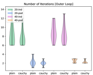
(a)

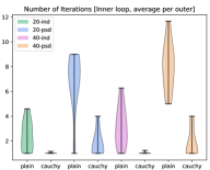
(b)

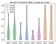
(c)

Figure 5: Computational results obtained with two variants of Algorithm 1 on test problem sets 20-ind, 20-psd, 40-ind, 40-psd. Both variants include BQP steps in ln. 14, the variant cauchy does and the variant plain does not include the SEARCH_CAUCHY_POINT routine after the LPCC step in ln. 7.

Both variants of Algorithm 1 converge in a modest number of outer iterations (less than 10). Similarly, the average number of inner iterations per outer iteration is small, which indicates that our trust region update strategy is efficient. In comparing the two variants, we note that the addition of the Cauchy step reduces the average number of inner iterations by a factor of 2–3 and slightly improves the number of outer iterations. Figure 5 shows violin plots comparing the performance of the two variants. The plots represent the distribution of the respective results on each of the four sets of problems. One can see that cauchy is slightly more efficient in terms of iteration numbers than plain and that both variants require a similar number of BQP iterations.

The number of major iterations of our approach is similar to or slightly less than the best NLP solver. Figure 6 shows violin plots for the largest problem instances (the results for the smaller instances are similar). We note that one run of SNOPT reached the maximum iteration limit of 200. Moreover, we have excluded four runs of MINOS of the set 40-psd, which stopped at infeasible points. We note that several runs of MINOS reported convergence to optimality but stopped with a first-order optimality tolerance higher than $10^{-5}$. To provide a realistic impression of the iteration counts, we have decided to include these runs in the plots.

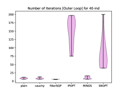
(a)

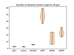
(b)

Figure 6: Number of outer iterations obtained with two variants of Algorithm 1 on test problem sets 20-ind, 20-psd, 40-ind, 40-psd compared with iterations of filterSQP, IPOPT, MINOS, and SNOPT. Both variants include BQP steps, the variant the variant cauchy does and the variant plain does not include the SEARCH_CAUCHY_POINT routine after the LPCC step.

The objective values and iteration numbers achieved with our implementation are comparable to those of the NLP solvers while the running times of our implementations are comparable to IPOPT but slower than the running times of filterSQP, MINOS and SNOPT. Although not always the case, the variant cauchy is often the slowest solver, but this may be attributed to the use of Python.

We provide detailed results in Appendix B. Specifically, Table 2 provides results of our two implementations on the quadratic problems. The rows of the table are the test problem instances with the names introduced above. For each test problem instance, the objective values for plain and cauchy are given as well as the number of outer, inner, and BQP iterations. Table 3 provides the major/outer iteration counts of the NLP solvers filterSQP, IPOPT, MINOS, and SNOPT and our implementations. Table 4 provides the running times of the NLP solvers and our implementations and Table 5 provides the achieved objective values for all solvers.

6.2 General Nonlinear Test Problems

We have also run our implementations cauchy and plain described above on twenty nonlinear test problems that are detailed in Appendix A.2. For the instances that are called 20-fletcher0, 20-fletcher1, 40-fletcher0, and 40-fletcher1 the reduced Hessian in the BQP subproblem is nearly singular and has a condition number larger than $10^{8}$ at the final iterate.

With the exception of the aforementioned degenerate instances, our implementation of Algorithm 1 always terminates with an iterate that satisfies a first-order optimality tolerance of $10^{-6}$ or less using relatively few iterations, approximately comparable to the test instances with quadratic objectives. Note that a first-order tolerance of $10^{-6}$ is reached by plain for 20-fletcher0, and 20-fletcher1 and by cauchy for 20-fletcher1, 40-fletcher0, and 40-fletcher1. The implementation terminates for the remaining instances because the trust region contracts to zero at the final iterate (our implementation stops after halving trust region radius 50 times), with a first-order error of around $10^{-5}$, which we count as a failure of our algorithm.

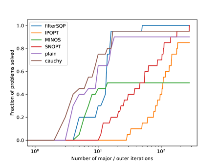
Figure 7: Number of major/outer iterations vs. fraction of problems solved for two variants of Algorithm 1 on the nonlinear test problem set compared with filterSQP, IPOPT, MINOS, and SNOPT. Both variants include BQP steps, the variant the variant cauchy does and the variant plain does not include the SEARCH_CAUCHY_POINT routine after the LPCC step.

We have run the same four NLP solvers on the general nonlinear test problems. The NLP solvers filterSQP and MINOS require a similar amount of outer iterations. The solvers SNOPT and IPOPT require significantly more iterations. IPOPT does not find a solution of sufficient first-order optimality for the degenerate instances within 3000 iterations. The solver MINOS terminates at infeasible points in three runs. In seven further runs, it shows a first-order error of $10^{-5}$ or higher on termination. We give a performance profile for the nonlinear test cases in Figure 7, where we count the aforementioned runs of IPOPT, MINOS, and our implementation as failures. We observe that our implementations are competitive with the best NLP solvers on the set of general nonlinear benchmark problems. As for the quadratic test problems, the objective values achieved with our implementation are comparable to those of the NLP solvers while the running time of our implementation plain is comparable to IPOPT but slower than the running times by filterSQP, MINOS and SNOPT. Again, the variant cauchy is often significantly slower than all other solvers.

We provide detailed results in Appendix B. Specifically, Table 6 provides detailed results of our two implementations on the quadratic problems. The rows of the table are the test problem instances with the names introduced above. For each test problem instance, the objective values for plain and cauchy computation are given as well as the number of outer, inner, and BQP iterations. Table 7 provides the major/outer iteration counts of the NLP solvers filterSQP, IPOPT, MINOS, and SNOPT and our implementations. Table 8 provides the running times of the NLP solvers and our implementations and Table 9 provides the achieved objective values of the NLP solvers and our implementations.

7 Conclusion and Extension

We have introduced a new sequential LPCC algorithm for bound-constrained MPCCs and shown that it converges to a B-stationary point. Such an approach can be used as a (nonsmooth) subproblem solver for general MPCCs. Our approach is shown to be competitive with state-of-the-art approaches for solving a collection of synthetic benchmark problems. The outer and inner loops of the benchmarked variants plain and cauchy of Algorithm 1 have been implemented in Python; switching to a different language may result in some performance improvements. We also believe that a more efficient implementation of the SEARCH_CAUCHY_POINT procedure would reduce the current gap in running times between the plain and cauchy variants.

To test the algorithmic developments in the context of our motivation, we have implemented an augmented Lagrangian method based on [32, Section 17.4] that solves subproblems of the form (3) using Algorithm 1. We test this approach on the nash1 problem from MacMPEC. Compared to an augmented Lagrangian method that treats the complementarities as general nonlinear constraints, we observe a different qualitative behavior on this test instance. In particular, the penalty parameter exhibits a slower growth over the iterations and a different sequence of iterates is taken. Both methods converge to the same strongly stationary point. In particular, our approach reaches minimal values for the constraint violation and stationarity measure after $4$ iterations at a penalty parameter value of $10^{3}$; the method that handles the complementarity constraint as a general nonlinear constraint reaches minimal values for constraint violation and stationarity measure after $8$ iterations at a penalty parameter value of $10^{7}$. See Appendix C for more detailed results and plots.

We note that it is straightforward to extend the developments of the preceding sections to formulations of complementarity-constrained problems of the form

$$\begin{aligned} \min_{x}\ &f(x)\\ \text{s.t.\ }&\ell_{0}\leq x_{0}\leq u_{0},\\ &\ell_{1}\leq x_{1}\leq u_{1}\;\perp\;\ell_{2}\leq x_{2}\leq u_{2},\end{aligned}$$ (1)

where for all $i\in\{1,\ldots,n_{1}\}$ exactly two of $\{\ell_{1,i},u_{1,i},\ell_{2,i},u_{2,i}\}$ are finite. This format allows more general mixed-complementarity expressions and mimics the definition of complementarity constraints in AMPL [13]. We tabulate two such types of complementarity formulations and sketch their active sets in Table 1. Other general forms are easily derived by swapping components between $x_{1}$ and $x_{2}$, shifting bounds, or negating variables. We note that we do not reformulate these complementarity constraints using slack variables, because such a reformulation would introduce additional linear constraints, making it harder to apply our trust region algorithm.

Table 1: Different types of complementarity constraints per coordinate pair $(x_{1,i},x_{2,i})$: short notation, description of feasible set, and sketch of the feasible set. The coordinate index is omitted.

	Short notation	Feasible set	Sketch
(a)	$\ell_{1}\leq x_{1}\leq u_{1}\perp x_{2}$	$\ell_{1}\leq x_{1}\leq u_{1}$, $x_{2}\in\left\{\begin{aligned} &:&x_{1}=u_{1}\end{aligned}\right.$
(b)	$\ell_{1}\leq x_{1}\perp x_{2}\leq u_{2}$	$\ell_{1}\leq x_{1}$, $x_{2}\leq u_{2}$, $(x_{1}-\ell_{1})(u_{2}-x_{2})\leq 0$

The trust region subproblem corresponding to general LPCCs is given by

$$\mbox{G-LPCC}(x,\Delta)\left\{\begin{array}[]{ll}\displaystyle\mathop{\rm minimize}_{d}&\nabla f(x)^{T}d\\ \textnormal{subject\ to:}&l_{0}\leq x_{0}+d_{0}\leq u_{0}\\ &\ell_{1}\leq x_{1}+d_{1}\leq u_{1}\;\perp\;\ell_{2}\leq x_{2}+d_{2}\leq u_{2},\\ &\|d\|_{\infty}\leq\Delta,\end{array}\right.$$

where $\ell_{0}$, $\ell_{1}$, $\ell_{2}$, $u_{0}$, $u_{1}$, and $u_{2}$ satisfy the conditions in (1).

It is a straightforward exercise to show that the trust region subproblem G-LPCC$(x,\Delta)$ can be solved as efficiently as (2), again by considering all possible solutions for each index $i$ independently. The convergence results then follow from the sufficient reduction condition, which is unaffected by the form of the complementarity constraints.

Appendix A Description of Test Problems

Here, we briefly describe the two classes of test problems that we used in our computational experiments.

The problems were generated in Matlab and written out as AMPL model and data files. All problem instances, as well as the Matlab routine used to generate them are available at https://wiki.mcs.anl.gov/leyffer/index.php/BndMPCC.

A.1 Quadratic MPCCs

The quadratic test problems are of the form

$$\begin{aligned} \mathop{\rm minimize}_{x}\ &\frac{1}{2}x^{T}Hx+g^{T}x\\ \textnormal{subject\ to:}\ &\ell_{0}\leq x_{0}\leq u_{0},\\ &0\leq x_{1}\;\perp\;x_{2}\geq 0,\end{aligned}$$ (2)

where $x_{0}\in\mathbb{R}^{n_{0}}$, $x_{1},x_{2}\in\mathbb{R}^{n_{1}}$, $H$ is a symmetric sparse matrix with density $(n_{0}+2n_{1})^{2}/4$ whose entries are normally distributed, and $g$ is a vector in $\mathbb{R}^{n_{0}+2n_{1}}$ whose components are uniform random numbers in the range $[-10,10]$. The bounds $l_{0},u_{0}$ are uniform random numbers in the range $[-10,10]$ and $[0,20]$, and we ensure that $l_{0,i}<u_{0,i}$. We round all data to four digits, because we have observed that this makes the problems harder to solve. In addition, we believe that real-life problems are not typically described in terms of double precision data.

A.2 General Nonlinear MPCCs

We have also curated a set of nonquadratic test problems of the form (1) by adding bounds and complementarity constraints to some well-known nonlinear test problems. For each nonlinear function, we created two sets of instances by varying the indices in the complementarity constraints. In all cases, $n=n_{0}+2n_{1}$, with $n_{0}=n_{1}=20$ or $n_{0}=n_{1}=40$, is used in our experiments. All functions are taken from [1].

fletcher

$\displaystyle f(x)=\sum_{i=1}^{n-1}100\big{(}x_{i+1}-x_{i}+1-x_{i}^{2}\big{)}^{2}$

himmelblau

$\displaystyle f(x)=\sum_{i=1}^{n/2}\big{(}(x_{2i-1}+x_{2i}-11)^{2}+(x_{2i-1}+x_{2i}^{2}-7)^{2}\big{)}$

mccormick

$\displaystyle f(x)=\sum_{i=1}^{n-1}\big{(}-1.5x_{i}+2.5x_{i+1}+1+(x_{i}-x_{i+1})^{2}+\sin(x_{i}+x_{i+1})\big{)}$

powell

+

$\displaystyle f(x)=\sum_{i=1}^{n/4}\big{(}(x_{4i-3}+10x_{4i-2})^{2}+5(x_{4i-1}-x_{4i})^{2}+(x_{4i-2}-2x_{4i-1})^{4}+10(x_{4i-3}-x_{4i})^{4}\big{)}$

rosenbrock

$\displaystyle f(x)=\sum_{i=1}^{n-1}\big{(}100(x_{i+1}-x_{i}^{2})^{2}+(1-x_{i})^{2}\big{)}$

For each function, we generated two instance classes with different complementarity constraints:

$$\text{Class 0:}\quad 0\leq x_{i}\; \perp \;x_{n_{1}+i}\geq 0,\quad\forall i\in 1,\ldots,n_{1}$$

$$\text{Class 1:}\quad 0\leq x_{2i-1}\; \perp \;x_{2i}\geq 0,\quad\forall i\in 1,\ldots,n_{1}.$$

For all nonlinear test problem instances , the lower bound $l_{0}$ on $x_{0}$ was set to zero in all coordinates. The upper bound $u_{0}$ on $x_{0}$, was set to $10^{8}$ in all coordinates.

Appendix B Detailed Computational Results

Table 2: Performance for Algorithm  1 with Algorithm 3, and with (cauchy) and without (plain) Algorithm 2 on 40 problem instances. (All first-order optimality measures are less than $10^{-13}$.) For each problem instance, boldface numbers indicate the algorithm that delivered the best (lowest) objective values and (total) iteration counts.

Prob-Inst.	Obj. val.		outer iters		total inner iters		BQP iters
	plain	cauchy	plain	cauchy	plain	cauchy	plain	cauchy
20-ind-0	-6459.47	-6459.47	10	8	46	8	28	24
20-ind-1	-7373.48	-7135.19	14	12	28	14	30	26
20-ind-2	-2618.47	-2538.46	6	6	8	6	13	13
20-ind-3	-3115.40	-3115.40	8	7	24	7	18	17
20-ind-4	-6272.72	-6219.23	8	8	12	8	16	18
20-ind-5	-2829.78	-2748.66	6	7	8	7	13	16
20-ind-6	-8374.58	-8374.58	11	10	31	10	22	20
20-ind-7	-1588.59	-1588.59	6	6	20	6	14	13
20-ind-8	-2045.32	-2045.32	8	7	30	7	17	15
20-ind-9	-5622.22	-5622.22	6	6	6	6	13	13
20-psd-0	1147.55	1147.55	2	2	12	4	4	4
20-psd-1	1043.67	1043.67	2	2	16	2	4	4
20-psd-2	1772.49	1772.49	2	2	14	4	4	4
20-psd-3	566.63	566.63	1	1	1	1	2	2
20-psd-4	896.98	898.00	2	2	18	6	4	4
20-psd-5	1507.17	1507.17	2	2	12	2	4	4
20-psd-6	751.21	751.21	4	3	36	3	8	6
20-psd-7	2050.00	2050.00	2	2	16	8	4	4
20-psd-8	1109.89	1109.89	3	2	25	2	7	6
20-psd-9	1090.73	1090.73	2	2	14	4	5	5
40-ind-0	-7999.59	-7997.27	6	7	6	7	12	15
40-ind-1	-17702.74	-17702.74	11	10	45	10	25	22
40-ind-2	-23716.62	-23462.24	8	7	16	7	16	16
40-ind-3	-7710.66	-7589.43	7	6	17	6	14	12
40-ind-4	-13571.15	-17301.43	12	13	46	13	24	26
40-ind-5	-10395.51	-10395.51	9	8	31	8	19	16
40-ind-6	-4889.03	-4890.66	8	7	40	7	18	15
40-ind-7	-17301.07	-17147.55	9	10	19	10	18	21
40-ind-8	-14414.19	-14198.29	8	8	14	10	18	21
40-ind-9	-10073.14	-10073.14	11	8	69	8	22	16
40-psd-0	4009.29	4009.29	3	3	23	7	6	6
40-psd-1	4147.27	4147.27	3	2	29	2	7	4
40-psd-2	3105.85	3116.39	2	2	10	2	5	6
40-psd-3	4944.42	4944.42	3	2	35	2	8	5
40-psd-4	2452.84	2452.84	3	2	25	2	6	6
40-psd-5	2365.25	2365.25	3	2	29	2	7	6
40-psd-6	4035.26	4035.26	2	2	12	4	4	5
40-psd-7	3154.05	3154.05	2	3	12	11	6	6
40-psd-8	2220.87	2220.87	2	2	16	8	4	4
40-psd-9	3657.14	3657.14	3	2	25	2	7	4

Table 3: Number of major/outer iterations for solving random instances of bound-constrained MPCCs (INF = Termination at infeasible point, F = Termination with violated optimality tolerance).

Prob-Inst.	Number of major/outer iterations
	plain	cauchy	filterSQP	IPOPT	MINOS	SNOPT
20-ind-0	10	8	6	108	F 07	41
20-ind-1	14	12	4	113	15	31
20-ind-2	6	6	5	79	7	25
20-ind-3	8	7	5	99	5	76
20-ind-4	8	8	6	108	F 20	68
20-ind-5	6	7	6	84	5	30
20-ind-6	11	10	6	91	6	36
20-ind-7	6	6	5	51	6	34
20-ind-8	8	7	6	92	7	33
20-ind-9	6	6	5	91	7	41
20-psd-0	2	2	6	43	F 18	15
20-psd-1	2	2	5	50	6	18
20-psd-2	2	2	5	39	6	15
20-psd-3	1	1	5	40	F 19	18
20-psd-4	2	2	5	43	F 18	16
20-psd-5	2	2	6	38	F 18	17
20-psd-6	4	3	5	42	7	19
20-psd-7	2	2	5	42	16	15
20-psd-8	3	2	5	42	14	19
20-psd-9	2	2	6	48	7	30
40-ind-0	6	7	6	132	7	F 200
40-ind-1	11	10	5	163	6	64
40-ind-2	8	7	6	96	F 15	47
40-ind-3	7	6	6	175	8	54
40-ind-4	12	13	6	178	7	118
40-ind-5	9	8	5	197	F 16	47
40-ind-6	8	7	6	75	F 07	39
40-ind-7	9	10	6	182	F 16	78
40-ind-8	8	8	6	167	F 15	122
40-ind-9	11	8	5	117	7	74
40-psd-0	3	3	6	49	19	27
40-psd-1	3	2	6	59	7	20
40-psd-2	2	2	6	43	24	23
40-psd-3	3	2	5	46	6	22
40-psd-4	3	2	6	54	INF	19
40-psd-5	3	2	6	48	INF	31
40-psd-6	2	2	6	46	20	17
40-psd-7	2	3	6	47	INF	25
40-psd-8	2	2	5	57	INF	21
40-psd-9	3	2	6	37	7	24

Table 4: Run times (seconds) for Algorithm  1 with Algorithm 3, and with (cauchy) and without (plain) Algorithm 2 as well as the NLP solvers on 40 problem instances (INF = Termination at infeasible point, F = Termination with violated optimality tolerance).

Prob-Inst.	Run times (seconds)
	plain	cauchy	filterSQP	IPOPT	MINOS	SNOPT
20-ind-0	$0.039$	$0.098$	$0.0053$	$0.066$	F 0.01	$0.03$
20-ind-1	$0.046$	$0.12$	$0.0027$	$0.073$	$0.01$	$0.02$
20-ind-2	$0.019$	$0.059$	$0.0025$	$0.040$	$0.01$	$0.01$
20-ind-3	$0.028$	$0.076$	$0.0024$	$0.058$	$0.01$	$0.03$
20-ind-4	$0.024$	$0.092$	$0.0030$	$0.063$	F 0.01	$0.04$
20-ind-5	$0.019$	$0.083$	$0.0037$	$0.041$	$0.01$	$0.02$
20-ind-6	$0.039$	$0.12$	$0.0036$	$0.055$	$0.01$	$0.03$
20-ind-7	$0.021$	$0.059$	$0.0027$	$0.028$	$0.01$	$0.02$
20-ind-8	$0.030$	$0.066$	$0.0035$	$0.059$	$0.01$	$0.02$
20-ind-9	$0.018$	$0.093$	$0.0032$	$0.050$	$0.01$	$0.03$
20-psd-0	$0.0093$	$0.020$	$0.0030$	$0.027$	F 0.01	$0.01$
20-psd-1	$0.010$	$0.026$	$0.0034$	$0.029$	$0.01$	$0.01$
20-psd-2	$0.0098$	$0.027$	$0.0047$	$0.019$	$0.01$	$0.01$
20-psd-3	$0.0036$	$0.016$	$0.0033$	$0.011$	F 0.01	$0.01$
20-psd-4	$0.010$	$0.021$	$0.0031$	$0.024$	F 0.03	$0.01$
20-psd-5	$0.0092$	$0.021$	$0.0037$	$0.024$	F 0.01	$0.01$
20-psd-6	$0.022$	$0.041$	$0.0032$	$0.024$	$0.01$	$0.01$
20-psd-7	$0.0098$	$0.026$	$0.0029$	$0.022$	$0.01$	$0.01$
20-psd-8	$0.016$	$0.023$	$0.0033$	$0.027$	$0.02$	$0.01$
20-psd-9	$0.010$	$0.029$	$0.0044$	$0.029$	$0.01$	$0.02$
40-ind-0	$0.058$	$0.24$	$0.016$	$0.23$	$0.03$	F 0.67
40-ind-1	$0.12$	$0.38$	$0.011$	$0.278$	$0.02$	$0.04$
40-ind-2	$0.082$	$0.41$	$0.016$	$0.18$	F 0.03	$0.03$
40-ind-3	$0.075$	$0.25$	$0.014$	$0.32$	$0.03$	$0.04$
40-ind-4	$0.13$	$0.40$	$0.016$	$0.34$	$0.04$	$0.08$
40-ind-5	$0.12$	$0.35$	$0.012$	$0.36$	F 0.03	$0.03$
40-ind-6	$0.087$	$0.27$	$0.013$	$0.12$	F 0.03	$0.03$
40-ind-7	$0.093$	$0.39$	$0.015$	$0.33$	F 0.05	$0.05$
40-ind-8	$0.082$	$0.34$	$0.014$	$0.305$	F 0.04	$0.08$
40-ind-9	$0.13$	$0.38$	$0.013$	$0.20$	$0.03$	$0.05$
40-psd-0	$0.038$	$0.10$	$0.016$	$0.069$	$0.05$	$0.02$
40-psd-1	$0.040$	$0.080$	$0.016$	$0.087$	$0.03$	$0.02$
40-psd-2	$0.024$	$0.081$	$0.015$	$0.068$	$0.18$	$0.02$
40-psd-3	$0.043$	$0.093$	$0.013$	$0.059$	$0.02$	$0.02$
40-psd-4	$0.040$	$0.077$	$0.017$	$0.085$	INF	$0.02$
40-psd-5	$0.041$	$0.11$	$0.019$	$0.062$	INF	$0.03$
40-psd-6	$0.023$	$0.081$	$0.014$	$0.061$	$0.05$	$0.01$
40-psd-7	$0.025$	$0.13$	$0.018$	$0.060$	INF	$0.02$
40-psd-8	$0.026$	$0.11$	$0.015$	$0.070$	INF	$0.02$
40-psd-9	$0.038$	$0.086$	$0.016$	$0.053$	$0.03$	$0.02$

Table 5: Achieved objective values for Algorithm  1 with Algorithm 3, and with (cauchy) and without (plain) Algorithm 2 as well as the NLP solvers on 40 problem instances (INF = Termination at infeasible point, F = Termination with violated optimality tolerance). For each problem instance, the lowest achieved objective values are printed in boldface.

Prob-Inst.	Achieved objective value
	plain	cauchy	filterSQP	IPOPT	MINOS	SNOPT
20-ind-0	-6459.47	-6459.47	-7582.63	-7550.90	F -7582.63	-6459.47
20-ind-1	-7373.48	-7135.19	-7373.48	-7135.19	-7334.84	-7336.22
20-ind-2	-2618.47	-2538.46	-2618.47	-2627.96	-3098.27	-2594.18
20-ind-3	-3115.40	-3115.40	-3038.25	-2953.03	-2946.15	-3115.40
20-ind-4	-6272.72	-6219.23	-8735.77	-7648.74	F -8370.13	-7819.34
20-ind-5	-2829.78	-2748.66	-2623.97	-2108.59	-2131.34	-2116.81
20-ind-6	-8374.58	-8374.58	-8172.41	-8374.58	-8374.58	-8374.58
20-ind-7	-1588.59	-1588.59	-1923.79	-1589.24	-1800.37	-1588.59
20-ind-8	-2045.32	-2045.32	-1969.94	-1970.99	-1963.62	-1969.94
20-ind-9	-5622.22	-5622.22	-3245.52	-5399.08	-3098.11	-5622.22
20-psd-0	1147.55	1147.55	1147.69	1147.55	F 1147.88	1147.55
20-psd-1	1043.67	1043.67	1043.67	1043.67	1043.67	1043.67
20-psd-2	1772.49	1772.49	1772.49	1772.49	1772.49	1772.49
20-psd-3	566.63	566.63	564.89	564.89	F 565.63	564.89
20-psd-4	896.98	898.00	896.98	896.98	F 897.95	896.98
20-psd-5	1507.17	1507.17	1487.97	1487.97	F 1488.45	1489.83
20-psd-6	751.21	751.21	725.97	725.97	725.97	725.97
20-psd-7	2050.00	2050.00	2050.00	2050.00	2050.00	2050.00
20-psd-8	1109.89	1109.89	1109.89	1109.89	1109.89	1109.89
20-psd-9	1090.73	1090.73	1075.17	1075.23	1075.17	1081.99
40-ind-0	-7999.59	-7997.27	-8254.03	-8089.13	-8197.27	F -8137.61
40-ind-1	-17702.74	-17702.74	-17891.48	-17702.74	-17970.51	-17702.74
40-ind-2	-23716.62	-23462.24	-23315.13	-22970.72	F -22994.94	-23117.33
40-ind-3	-7710.66	-7589.43	-7866.74	-7589.43	-7735.33	-7800.41
40-ind-4	-13571.15	-17301.43	-14451.51	-14746.28	-14746.28	-16984.42
40-ind-5	-10395.51	-10395.51	-10668.66	-10668.66	F -10456.41	-10672.87
40-ind-6	-4889.03	-4890.66	-4851.44	-4728.64	F -4767.99	-5073.21
40-ind-7	-17301.07	-17147.55	-20378.55	-17361.50	F -17412.02	-17835.51
40-ind-8	-14414.19	-14198.29	-15355.83	-14339.09	F -13804.13	-14309.26
40-ind-9	-10073.14	-10073.14	-10848.63	-10732.42	-10848.63	-10633.96
40-psd-0	4009.29	4009.29	4002.46	4002.77	4005.18	4009.60
40-psd-1	4147.27	4147.27	4130.51	4130.51	4130.51	4147.27
40-psd-2	3105.85	3116.39	3105.85	3105.85	3106.95	3105.85
40-psd-3	4944.42	4944.42	4941.11	4941.11	4941.11	4941.11
40-psd-4	2452.84	2452.84	2446.08	2450.67	INF	2452.84
40-psd-5	2365.25	2365.25	2364.77	2364.77	INF	2365.25
40-psd-6	4035.26	4035.26	4035.23	4035.23	4035.23	4035.26
40-psd-7	3154.05	3154.05	3152.99	3152.99	INF	3154.05
40-psd-8	2220.87	2220.87	2220.35	2222.91	INF	2220.32
40-psd-9	3657.14	3657.14	3657.14	3657.14	3657.14	3657.88

Table 6: Performance for Algorithm  1 with Algorithm 3, and with (cauchy) and without (plain) Algorithm 2 on nonlinear test instances. For each problem instance, the lowest (total) iteration numbers are printed in boldface.

Prob-Inst.	Obj. val.		outer iters		total inner iters		BQP iters
	plain	cauchy	plain	cauchy	plain	cauchy	plain	cauchy
20-fletcher0	$2246.86$	$2246.86$	6	8	184	366	16	17
20-fletcher1	$4046.86$	$4046.86$	14	13	228	129	44	40
20-himmelblau0	$826.29$	$826.29$	9	9	93	49	9	9
20-himmelblau1	$230.31$	$230.31$	9	8	93	58	9	8
20-mccormick0	$58.93$	$58.93$	3	3	21	23	3	2
20-mccormick1	$58.93$	$58.93$	4	3	60	23	4	2
20-powell0	$9.6\text{\times}{10}^{-10}$	$7.5\text{\times}{10}^{-10}$	17	16	449	364	37	35
20-powell1	$3.0\text{\times}{10}^{-9}$	$1.1\text{\times}{10}^{-18}$	15	6	441	12	28	7
20-rosenbrock0	$58.61$	$58.61$	3	2	81	40	4	2
20-rosenbrock1	$58.61$	$58.61$	3	2	83	40	4	2
40-fletcher0	$4246.86$	$4246.86$	9	4	445	72	18	8
40-fletcher1	$8046.86$	$8046.86$	18	16	512	222	48	39
40-himmelblau0	$1652.58$	$1652.58$	9	9	93	49	10	9
40-himmelblau1	$460.63$	$460.63$	9	8	91	58	9	8
40-mccormick0	$118.93$	$118.93$	3	3	21	23	3	2
40-mccormick1	$118.93$	$118.93$	4	3	60	23	4	2
40-powell0	$9.8\text{\times}{10}^{-9}$	$1.5\text{\times}{10}^{-9}$	16	16	396	364	35	35
40-powell1	$5.9\text{\times}{10}^{-9}$	$2.1\text{\times}{10}^{-18}$	15	6	441	12	28	7
40-rosenbrock0	$118.20$	$118.20$	3	2	81	40	4	2
40-rosenbrock1	$118.21$	$118.21$	3	2	83	40	4	2

Table 7: Number of major/outer iterations for solving instances of bound-constrained nonlinear MPCCs (INF = Termination at infeasible point, F = Termination with violated optimality tolerance).

Prob-Inst.	Number of major/outer iterations
	plain	cauchy	filterSQP	IPOPT	MINOS	SNOPT
20-fletcher-0	6	F 08	49	F 3000	F 07	45
20-fletcher-1	14	13	13	F 3000	F 08	62
20-himmelblau-0	7	7	13	107	7	277
20-himmelblau-1	9	8	13	28	F 05	20
20-mccormick-0	3	3	4	75	4	15
20-mccormick-1	4	3	4	116	5	11
20-powell-0	17	16	15	146	6	29
20-powell-1	15	6	15	60	13	25
20-rosenbrock-0	3	2	13	80	7	107
20-rosenbrock-1	3	2	9	105	INF	86
40-fletcher-0	F 09	4	12	F 3000	F 07	176
40-fletcher-1	F 18	16	13	144	F 09	110
40-himmelblau-0	9	9	11	102	F 03	140
40-himmelblau-1	9	8	13	32	F 03	22
40-mccormick-0	3	3	4	175	5	11
40-mccormick-1	4	3	4	133	5	10
40-powell-0	16	16	15	181	9	37
40-powell-1	15	6	15	49	6	54
40-rosenbrock-0	3	2	13	86	INF	102
40-rosenbrock-1	3	2	9	95	INF	54

Table 8: Run times (seconds) for Algorithm  1 with Algorithm 3, and with (cauchy) and without (plain) Algorithm 2 as well as the NLP solvers for solving instances of bound-constrained nonlinear MPCCs (INF = Termination at infeasible point, F = Termination with violated optimality tolerance).

Prob-Inst.	Run times (seconds)
	plain	cauchy	filterSQP	IPOPT	MINOS	SNOPT
20-fletcher-0	$0.061$	F 1.107	$0.013$	$0.625$	F 0.01	$0.05$
20-fletcher-1	$0.093$	$0.556$	$0.0048$	$0.637$	F 0.01	$0.06$
20-himmelblau-0	$0.045$	$0.251$	$0.0042$	$0.032$	$0.01$	$0.22$
20-himmelblau-1	$0.045$	$0.214$	$0.0038$	$0.010$	F 0.01	$0.03$
20-mccormick-0	$0.013$	$0.047$	$0.0015$	$0.029$	$0.00$	$0.01$
20-mccormick-1	$0.025$	$0.045$	$0.0015$	$0.040$	$0.00$	$0.01$
20-powell-0	$0.154$	$1.849$	$0.0048$	$0.044$	$0.01$	$0.05$
20-powell-1	$0.144$	$0.081$	$0.0052$	$0.011$	$0.01$	$0.03$
20-rosenbrock-0	$0.028$	$0.171$	$0.0057$	$0.027$	$0.01$	$0.12$
20-rosenbrock-1	$0.029$	$0.189$	$0.0050$	$0.031$	INF	$0.08$
40-fletcher-0	F 0.088	$0.323$	$0.013$	$0.801$	F 0.01	$0.26$
40-fletcher-1	F 0.324	$1.672$	$0.0091$	$0.057$	F 0.01	$0.13$
40-himmelblau-0	$0.104$	$0.609$	$0.010$	$0.032$	F 0.01	$0.16$
40-himmelblau-1	$0.103$	$0.517$	$0.010$	$0.015$	F 0.01	$0.03$
40-mccormick-0	$0.033$	$0.107$	$0.0025$	$0.071$	$0.01$	$0.01$
40-mccormick-1	$0.054$	$0.106$	$0.0023$	$0.062$	$0.01$	$0.01$
40-powell-0	$0.266$	$4.319$	$0.014$	$0.079$	$0.02$	$0.07$
40-powell-1	$0.264$	$0.206$	$0.015$	$0.016$	$0.01$	$0.12$
40-rosenbrock-0	$0.052$	$0.396$	$0.018$	$0.032$	INF	$0.27$
40-rosenbrock-1	$0.053$	$0.438$	$0.015$	$0.038$	INF	$0.18$

Table 9: Achieved objective values for Algorithm  1 with Algorithm 3, and with (cauchy) and without (plain) Algorithm 2 as well as the NLP solvers for solving instances of bound-constrained nonlinear MPCCs (INF = Termination at infeasible point, F = Termination with violated optimality tolerance). For each problem instance, the lowest achieved objective values are in boldface.

Prob-Inst.	Achieved objective value
	plain	cauchy	filterSQP	IPOPT	MINOS	SNOPT
20-fletcher-0	2246.86	F 2246.86	2246.86	2246.86	F 2246.86	2246.86
20-fletcher-1	4046.86	4046.86	4032.29	3930.27	F 3988.57	3988.57
20-himmelblau-0	826.29	826.29	826.29	1840.62	1840.63	1029.16
20-himmelblau-1	230.31	230.31	826.29	1422.27	F  954.29	1422.27
20-mccormick-0	58.93	58.93	58.93	58.93	58.93	59.92
20-mccormick-1	58.93	58.93	58.93	58.93	58.93	58.93
20-powell-0	9.6$\cdot 10^{-10}$	7.5$\cdot 10^{-10}$	3.2$\cdot 10^{-10}$	8.0$\cdot 10^{-8}$	6.6$\mathbf{\cdot 10^{-14}}$	1.3$\cdot 10^{-13}$
20-powell-1	3.0$\cdot 10^{-9}$	1.1$\mathbf{\cdot 10^{-18}}$	2.2$\cdot 10^{-10}$	8.7$\cdot 10^{-8}$	4.7$\cdot 10^{-15}$	6.5$\cdot 10^{-5}$
20-rosenbrock-0	58.60	58.60	55.88	58.39	40.06	44.02
20-rosenbrock-1	58.61	58.61	58.34	58.61	INF	58.39
40-fletcher-0	F 4246.86	4246.86	4246.86	4246.86	F 4246.86	4679.15
40-fletcher-1	F 8046.86	8046.86	8032.29	7784.54	F 7988.57	7959.42
40-himmelblau-0	1652.58	1652.58	1652.58	1754.02	F 5118.83	1754.02
40-himmelblau-1	460.63	460.63	1652.58	2844.54	F 4074.33	2844.54
40-mccormick-0	118.93	118.93	118.93	118.93	118.93	118.93
40-mccormick-1	118.93	118.93	118.93	118.93	118.93	118.93
40-powell-0	9.8$\cdot 10^{-9}$	1.5$\cdot 10^{-9}$	6.4$\cdot 10^{-10}$	5.9$\cdot 10^{-8}$	8.4$\mathbf{\cdot 10^{-13}}$	4.5$\cdot 10^{-10}$
40-powell-1	5.9$\cdot 10^{-9}$	2.1$\mathbf{\cdot 10^{-18}}$	4.4$\cdot 10^{-10}$	1.6$\cdot 10^{-7}$	2.7$\cdot 10^{-18}$	2.1$\cdot 10^{-8}$
40-rosenbrock-0	118.20	118.20	115.48	118.20	INF	113.51
40-rosenbrock-1	118.21	118.21	117.99	118.21	INF	117.99

Appendix C Example – Augmented Lagrangian Integration

To demonstrate one approach for integrating our algorithm into an augmented Lagrangian method, we have implemented the algorithm for bound- and equality-constrained NLPs from [32, Section 17.4] and replaced the subproblems by (3) as described in Section 1.

We demonstrate the observed behavior of such an approach on the nash1 problem from MacMPEC, which is stated (including slack variables) below:

$$\min_{x_{0},x_{1},x_{2}} \frac{1}{2}\left((x_{0,1}-x_{0,3})^{2}+(x_{0,2}-x_{0,4})^{2}\right)$$

s.t. $$x_{1,1}=15-x_{0,2}-x_{0,3},\ \ x_{1,2}=15-x_{0,1}+x_{0,4},$$

$$x_{2,1}=34-2x_{0,3}-\frac{8}{3}x_{0,4},\ \ x_{2,2}=24.25-1.25x_{0,3}-2x_{0,4},$$

$$0\leq x_{1}\perp x_{2}\geq 0,$$

$$0\leq x_{0,1}\leq 10,\ \ 0\leq x_{0,2}\leq 10.$$

The augmented Lagrangian method converges to the strongly stationary point $(x_{0}^{T},x_{1}^{T},x_{2}^{T})=(5,9,5,9,1,19,0,0)$ within four iterations, where the constraints are satisfied to an accuracy of $10^{-10}$ in the $\ell_{2}$-norm and strong stationarity (computed as the $\ell_{\infty}$-norm residual of the gradient of the Lagrangian projected to bounds and complementarity conditions) is satisfied to an accuracy of $10^{-10}$ as well. Tightening these criteria further results in numerical instabilities in later iterations (multipliers and penalty parameters start diverging while the obtained point does not move). To help demonstrate the iterations, we illustrate the convergence of the method in Figure 8.

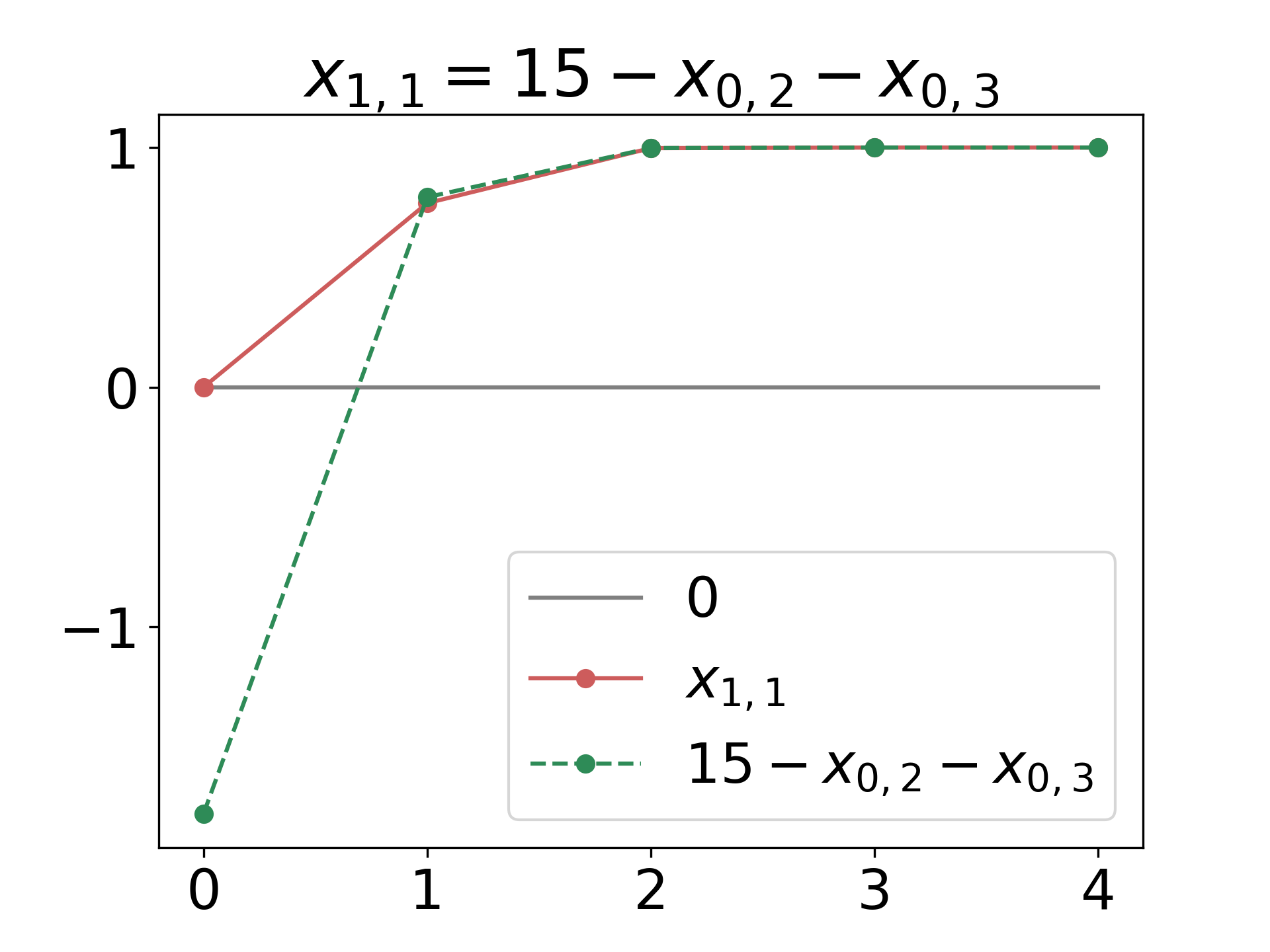
(a)

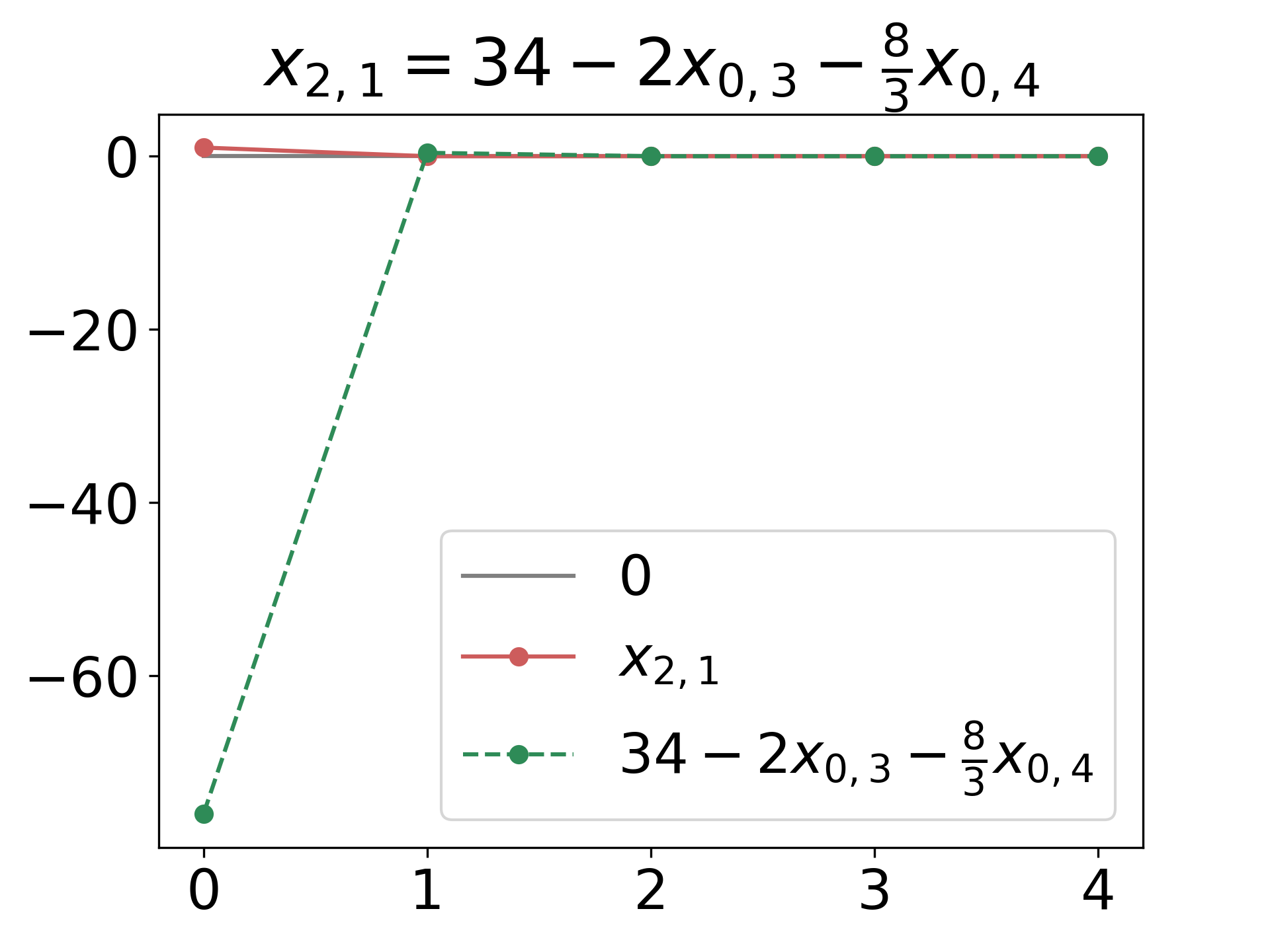
(b)

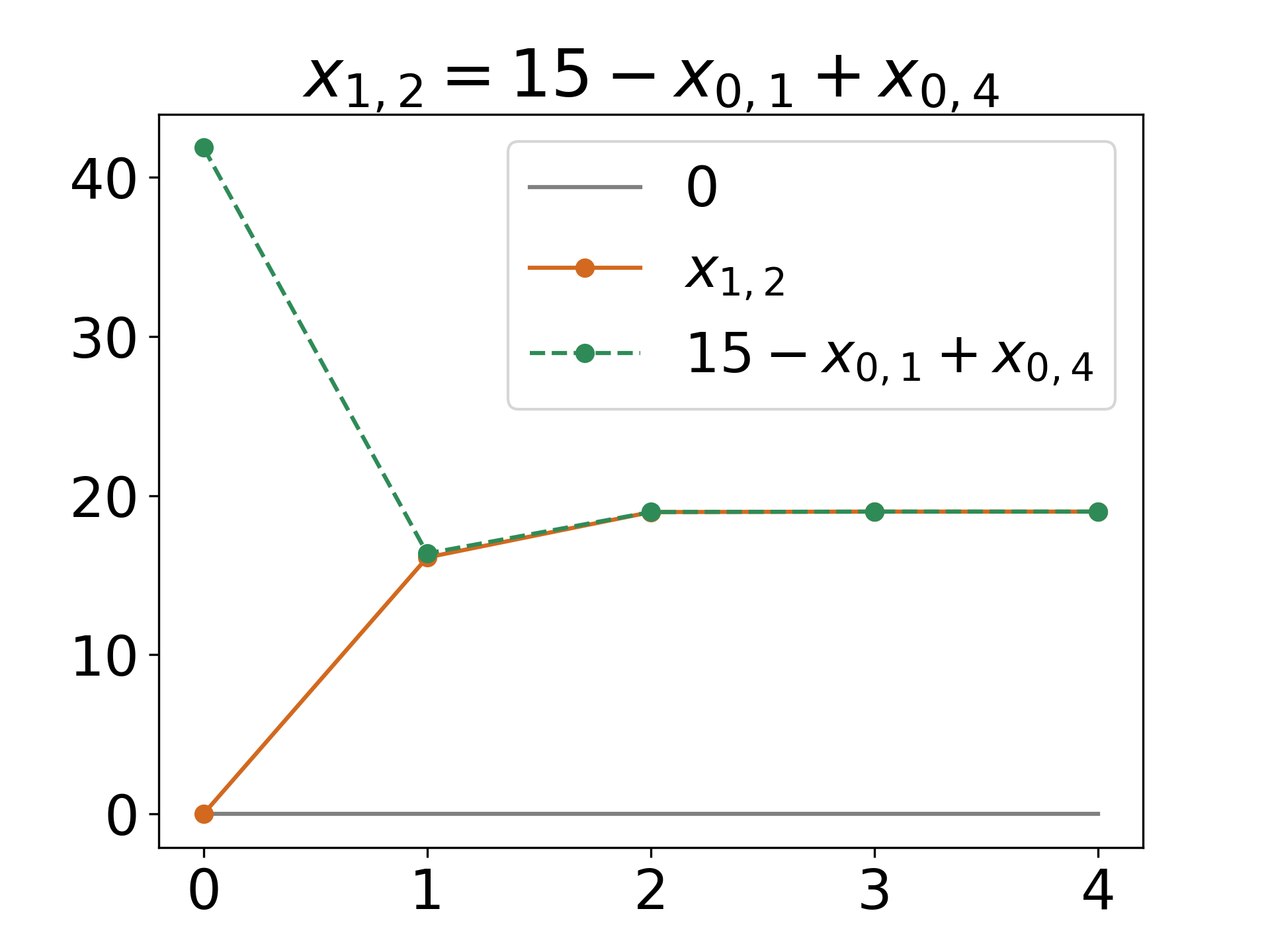
(c)

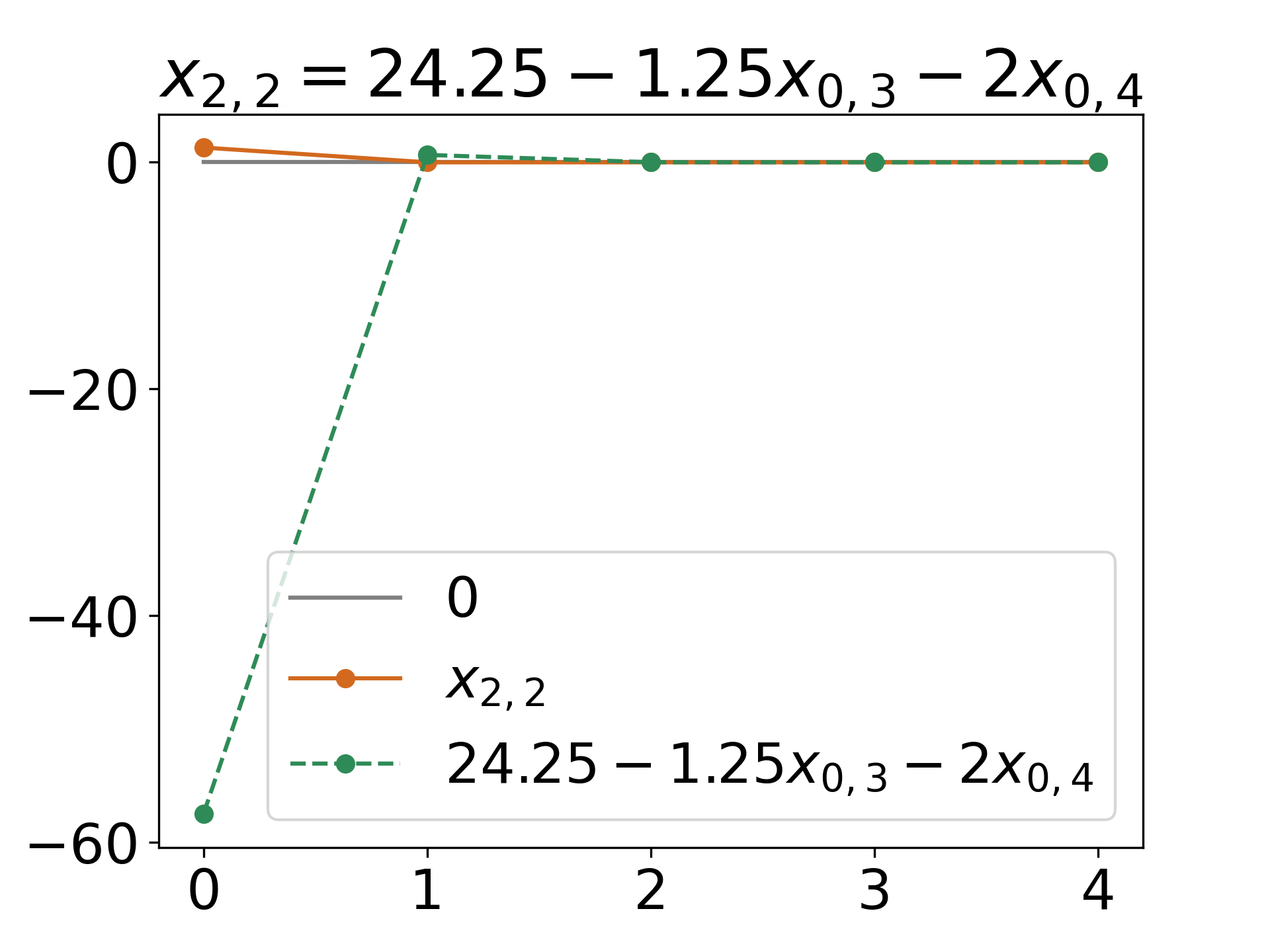
(d)

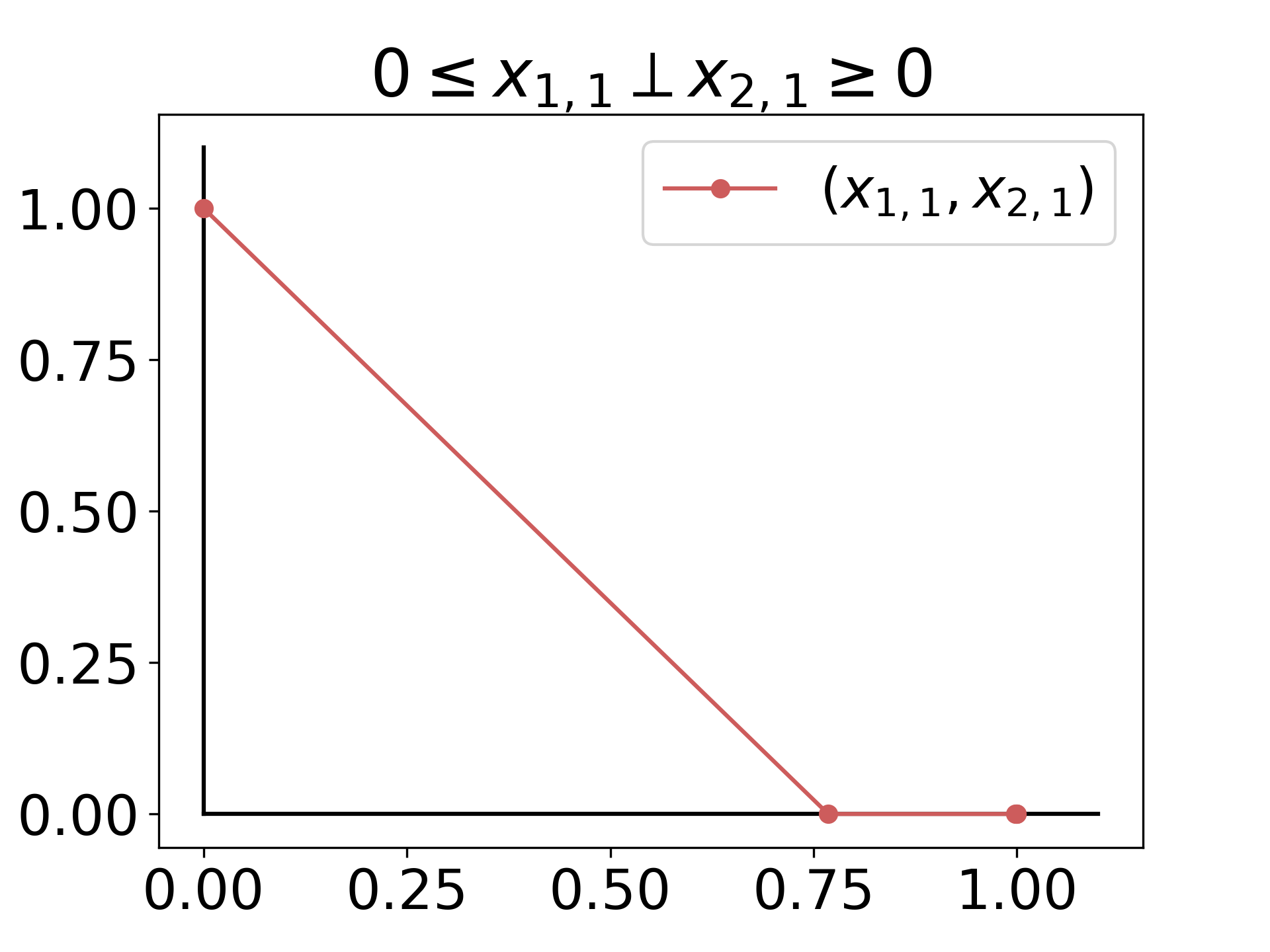
(e)

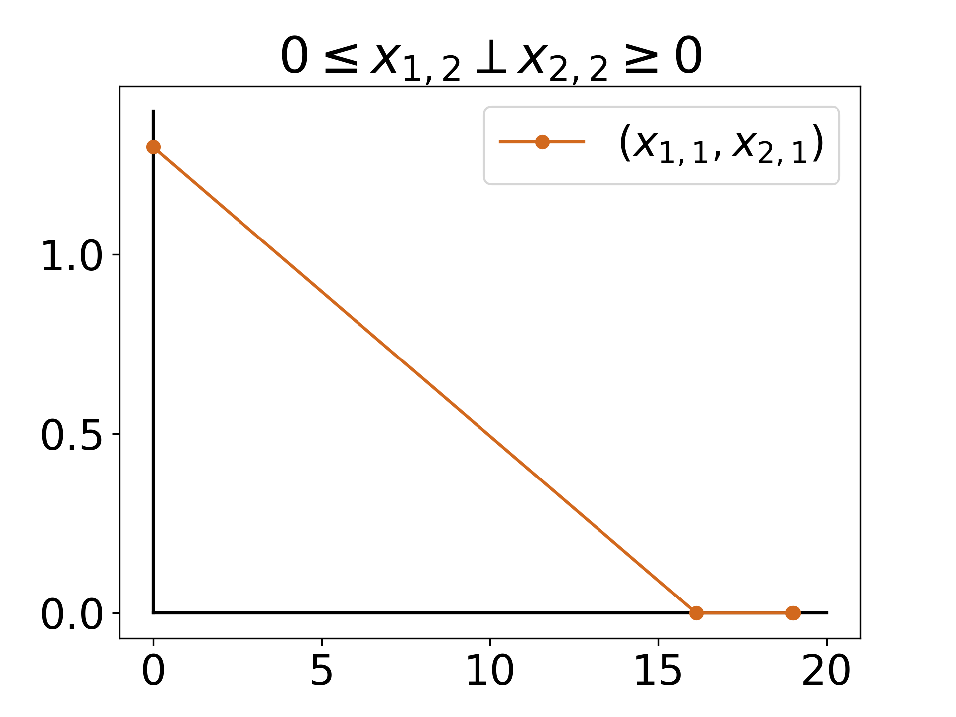
(f)

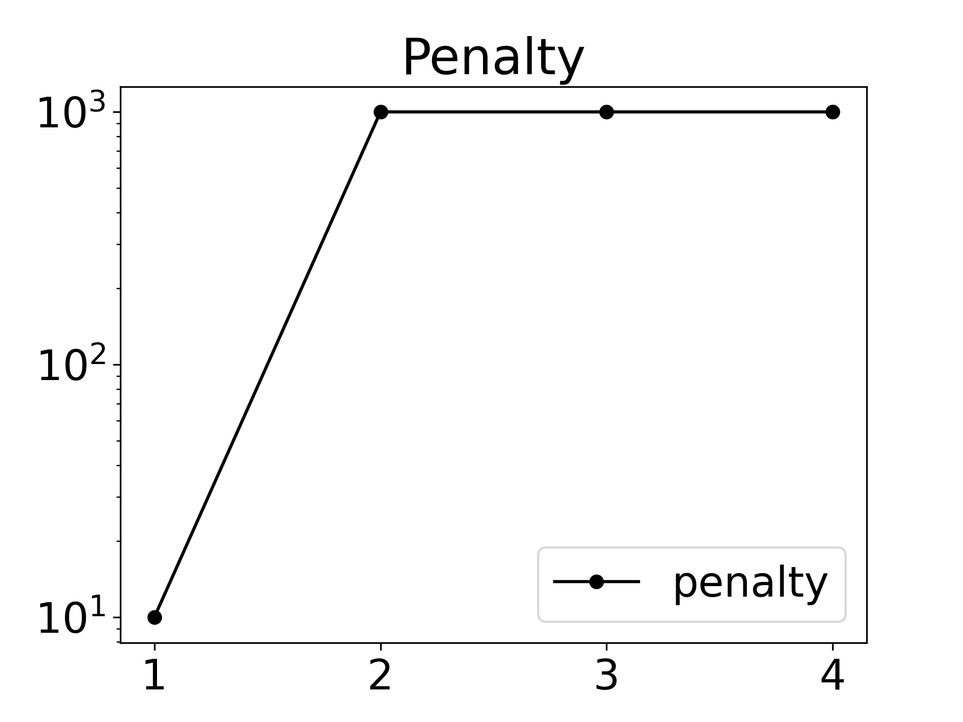
(g)

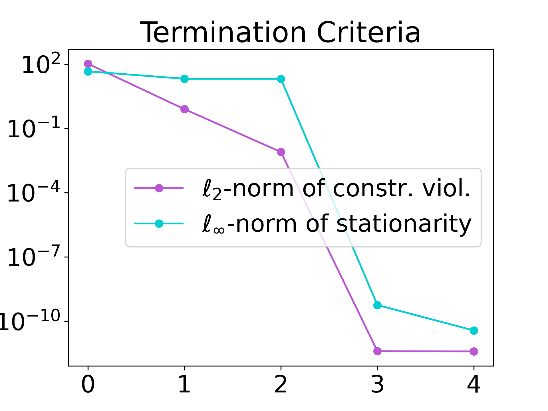
(h)

Figure 8: Visualization of the augmented Lagrangian method with nonsmooth subproblems, convergence of the constraints and slacks for the nonsmooth constraints over the iterations ((a)-(d) in top row), feasibility of the complementarity conditions ((e)-(f) in bottom row), penalty parameter over the iterations ((g) in bottom row) and Convergence of optimality and feasibility over the iterations ((h) in bottom row).

We compare this approach to an augmented Lagrangian method applied to a problem where the complementarity constraint $x_{1,i}x_{2,i}\leq 0$ is penalized in the objective. We use again the method from [32, Section 17.4] (just adapting the multiplier update for the inequality constraints), and use L-BFGS-B for the subproblem solves. We provide the same starting point and converge to the same point although we obtain a slightly worse accuracy of $10^{-7}$ and the algorithm takes more iterations. An analogous plot of Figure 8 is given in Figure 9. That our proposed method satisfies the complementarity constraints throughout all iterations is clearly visible.

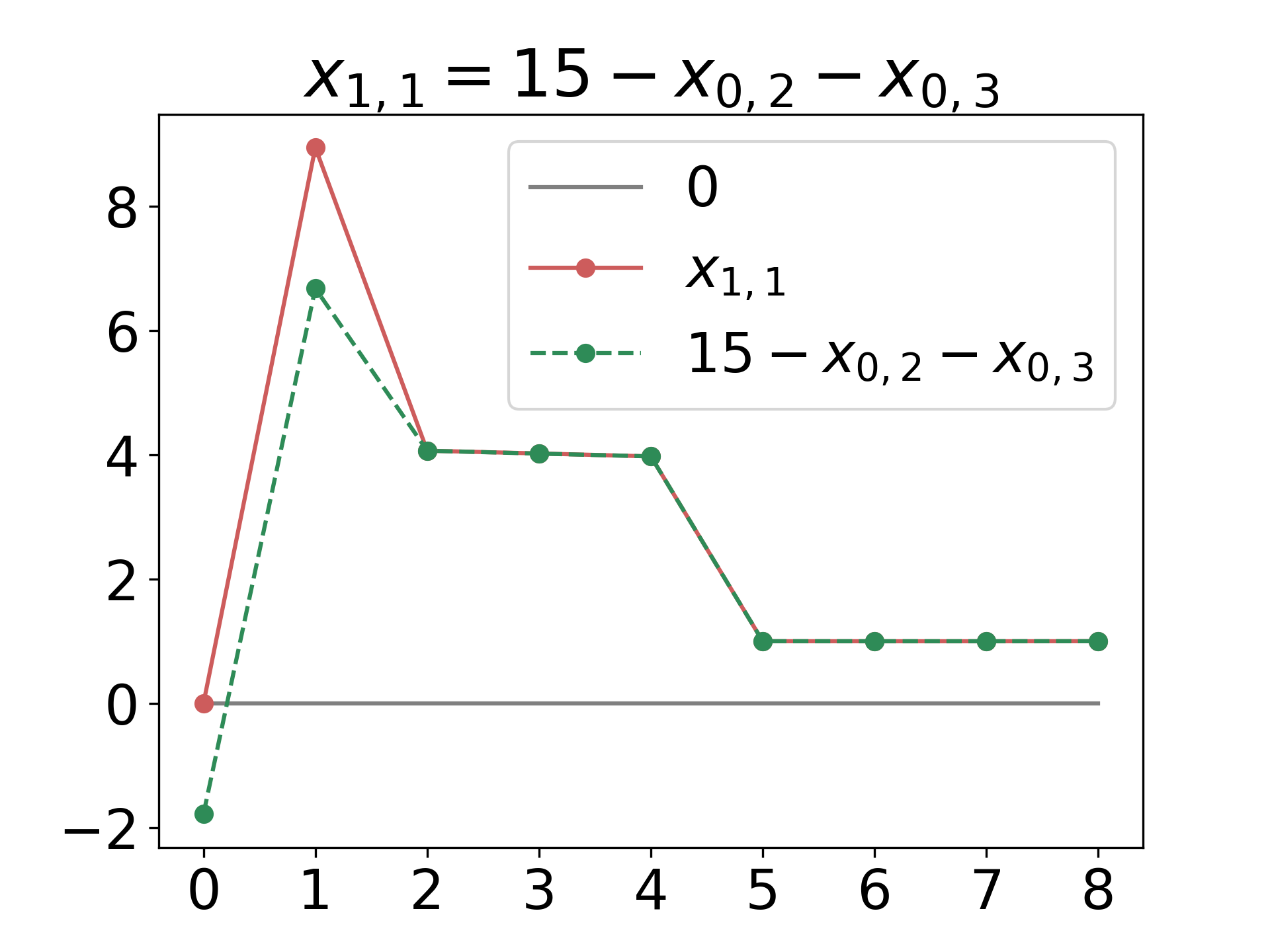
(a)

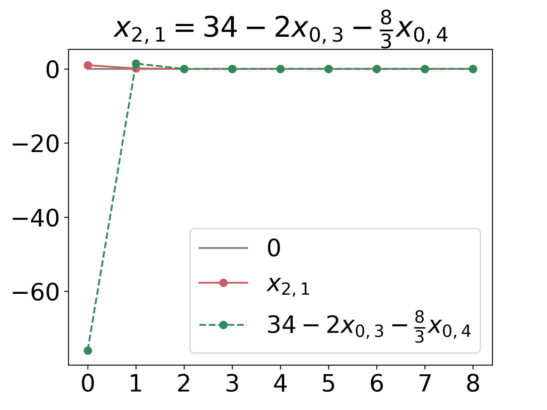
(b)

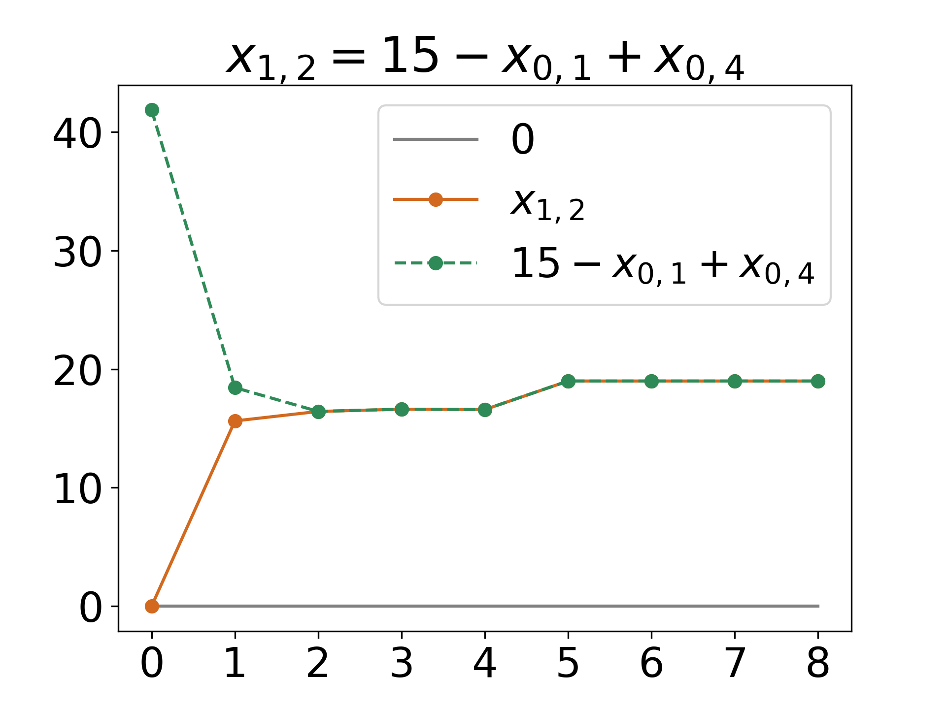
(c)

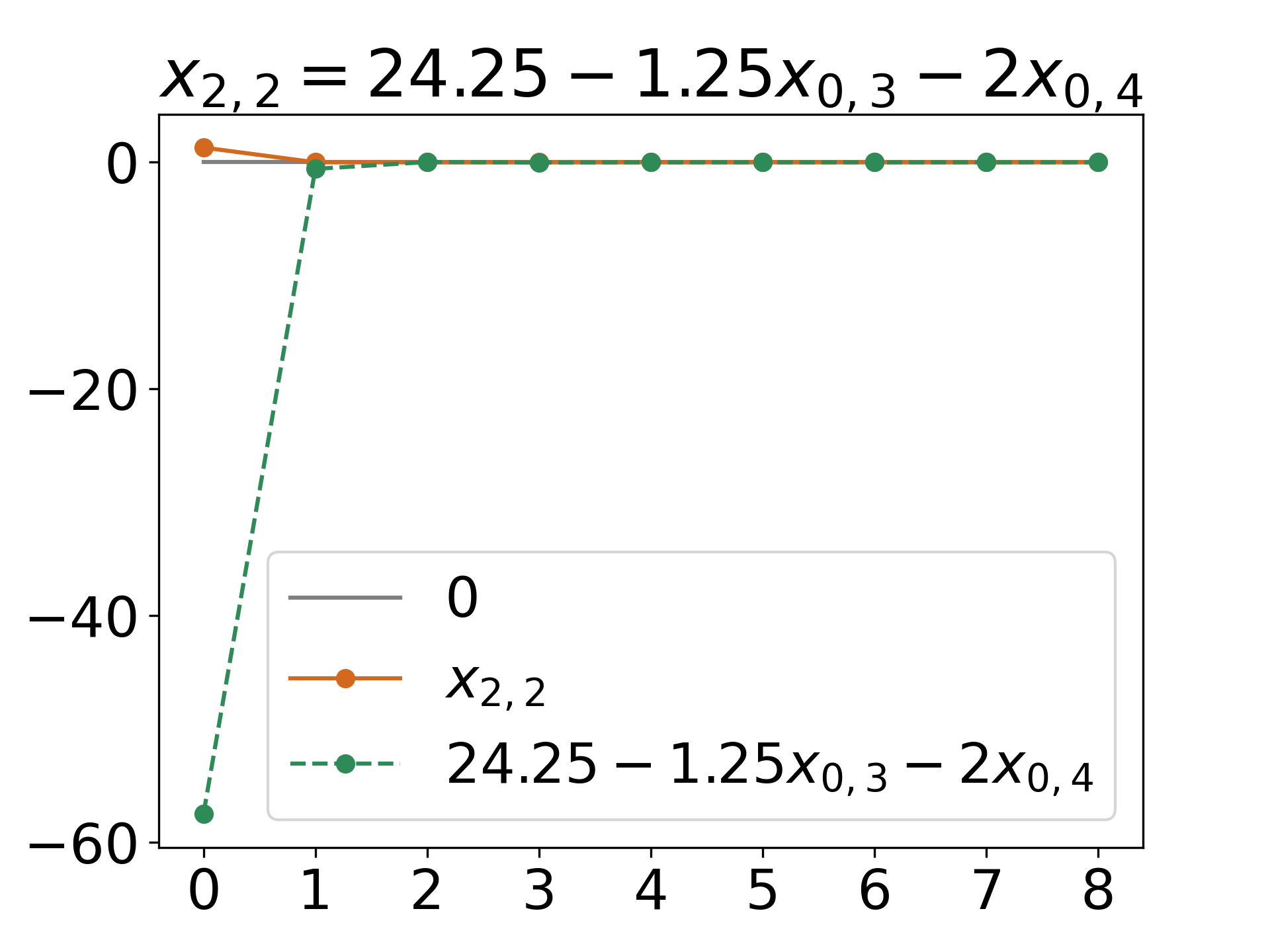
(d)

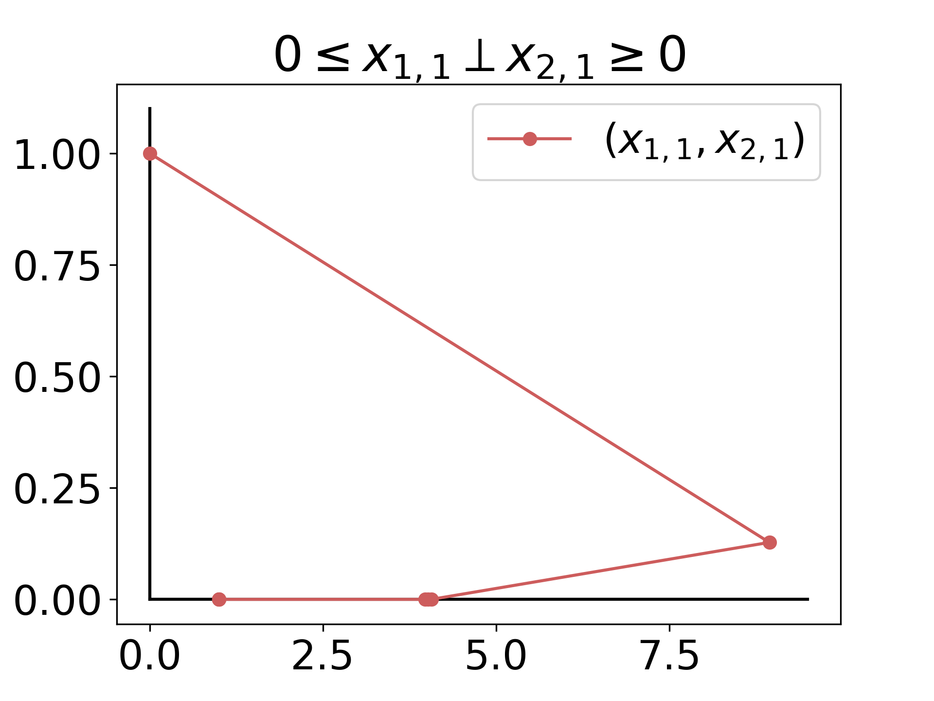
(e)

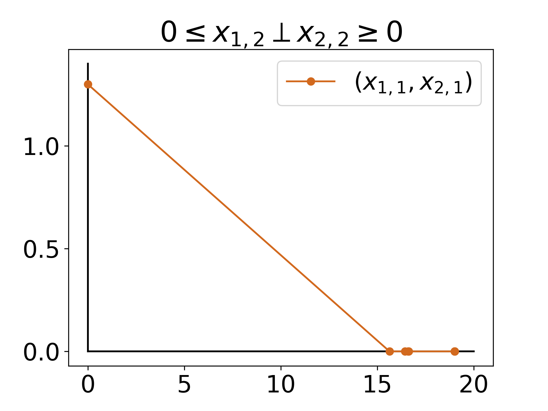
(f)

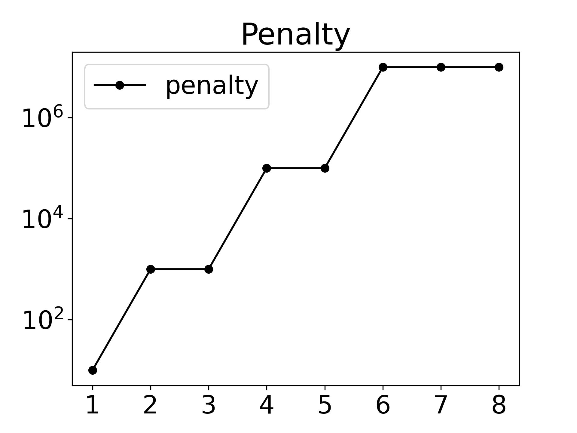
(g)

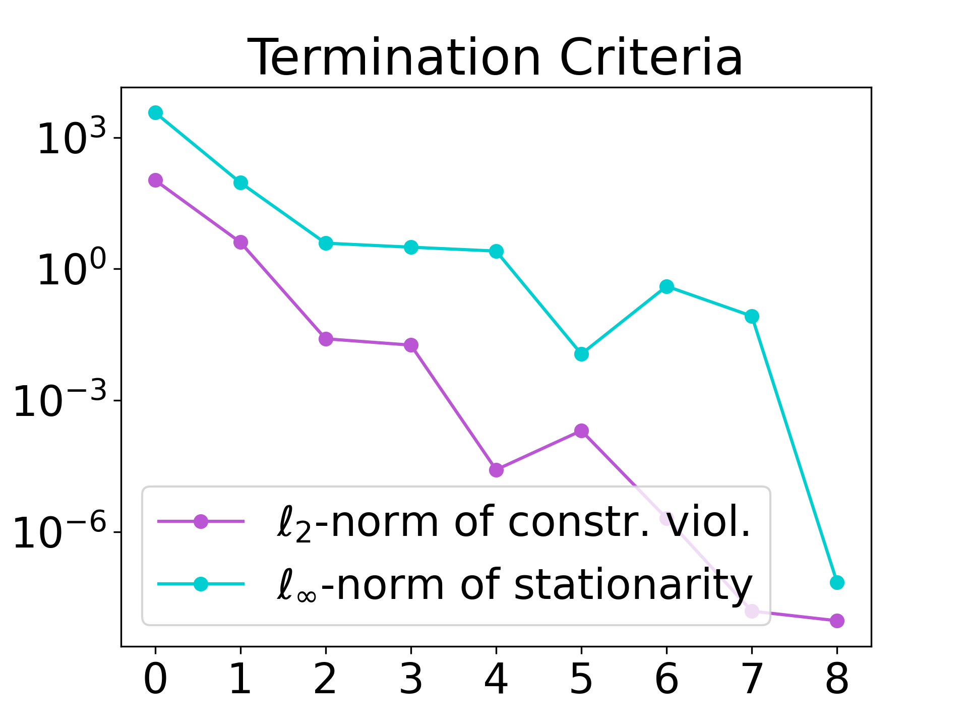
(h)

Figure 9: Visualization of the augmented Lagrangian method with complementarity constraints treated as general nonlinear constraints, convergence of the constraints and slacks for the nonsmooth constraints over the iterations ((a)-(d) in top row), feasibility of the complementarity conditions ((e)-(f) in bottom row), penalty parameter over the iterations ((g) in bottom row) and Convergence of optimality and feasibility over the iterations ((h) in bottom row).

The submitted manuscript has been created by UChicago Argonne, LLC, Operator of Argonne National Laboratory (“Argonne”). Argonne, a U.S. Department of Energy Office of Science laboratory, is operated under Contract No. DE-AC02-06CH11357. The U.S. Government retains for itself, and others acting on its behalf, a paid-up nonexclusive, irrevocable worldwide license in said article to reproduce, prepare derivative works, distribute copies to the public, and perform publicly and display publicly, by or on behalf of the Government. The Department of Energy will provide public access to these results of federally sponsored research in accordance with the DOE Public Access Plan http://energy.gov/downloads/doe-public-access-plan.

References

- [1] N. Andrei, An unconstrained optimization test functions collection, Advanced Modeling and Optimization, 10 (2008), pp. 147–161, https://camo.ici.ro/journal/vol10/v10a10.pdf.
- [2] E. G. Birgin, TANGO: Trustable Algorithms for Nonlinear General Optimization, Institute of Mathematics, Statistics and Scientific Computation, University of Campinas, Brazil, https://www.ime.usp.br/~egbirgin/tango/, 2005.
- [3] E. G. Birgin and J. M. Martínez, Practical Augmented Lagrangian Methods for Constrained Optimization, SIAM, 2014, https://doi.org/10.1137/1.9781611973365.
- [4] E. G. Birgin and J. M. Martínez, Improving ultimate convergence of an augmented Lagrangian method, Optimization Methods and Software, 23 (2008), pp. 177–195, https://doi.org/10.1080/10556780701577730.
- [5] R. H. Byrd, N. I. M. Gould, J. Nocedal, and R. A. Waltz, An algorithm for nonlinear optimization using linear programming and equality constrained subproblems, Mathematical Programming, Series B, 100 (2004), pp. 27–48, https://doi.org/10.1007/s10107-003-0485-4.
- [6] L. Chen and D. Goldfarb, An active-set method for mathematical programs with linear complementarity constraints, tech. report, Department of Industrial Engineering and Operations Research, Columbia University, 2007.
- [7] C. Chin and R. Fletcher, On the global convergence of an SLP-filter algorithm that takes EQP steps, Mathematical Programming, 96 (2003), pp. 161–177, https://doi.org/10.1007/s10107-003-0378-6.
- [8] A. R. Conn, N. I. M. Gould, and P. L. Toint, LANCELOT: A Fortran package for large-scale nonlinear optimization (Release A), Springer Verlag, Heidelberg, New York, 1992, https://doi.org/10.1007/978-3-662-12211-2.
- [9] A. R. Conn, N. I. M. Gould, and P. L. Toint, Numerical experiments with the LANCELOT package (Release A) for large–scale nonlinear optimization, Mathematical Programming, 73 (1996), pp. 73–110, https://doi.org/10.1007/bf02592099.
- [10] R. W. Cottle and G. B. Dantzig, Complementary pivot theory of mathematical programming, Linear Algebra and Its Applications, 1 (1968), pp. 103–125, https://doi.org/10.1016/0024-3795(68)90052-9.
- [11] F. E. Curtis, H. Jiang, and D. P. Robinson, An adaptive augmented Lagrangian method for large-scale constrained optimization, Mathematical Programming, 152 (2015), pp. 201–245, https://doi.org/10.1007/s10107-014-0784-y.
- [12] H. Fang, S. Leyffer, and T. S. Munson, A pivoting algorithm for linear programming with linear complementarity constraints, Optimization Methods and Software, 27 (2012), pp. 89–114, https://doi.org/10.1080/10556788.2010.512956.
- [13] M. C. Ferris, R. Fourer, and D. M. Gay, Expressing complementarity problems in an algebraic modeling language and communicating them to solvers, SIAM Journal on Optimization, 9 (1999), pp. 991–1009, https://doi.org/10.1137/s105262349833338x.
- [14] M. C. Ferris and T. S. Munson, Interfaces to PATH 3.0: Design, implementation and usage, Computational Optimization and Applications, 12 (1999), pp. 207–227, https://doi.org/10.1023/A:1008636318275.
- [15] M. L. Flegel and C. Kanzow, Abadie-type constraint qualification for mathematical programs with equilibrium constraints, Journal of Optimization Theory and Applications, 124 (2005), pp. 595–614, https://doi.org/10.1007/s10957-004-1176-x.
- [16] R. Fletcher and E. S. de la Maza, Nonlinear programming and nonsmooth optimization by successive linear programming, Mathematical Programming, 43 (1989), pp. 235–256, https://doi.org/10.1007/bf01582292.
- [17] R. Fletcher and S. Leyffer, Nonlinear programming without a penalty function, Mathematical Programming, 91 (2002), pp. 239–269, https://doi.org/10.1007/s101070100244.
- [18] R. Fletcher and S. Leyffer, Solving mathematical program with complementarity constraints as nonlinear programs, Optimization Methods and Software, 19 (2004), pp. 15–40, https://doi.org/10.1080/10556780410001654241.
- [19] R. Fletcher, S. Leyffer, D. Ralph, and S. Scholtes, Local convergence of SQP methods for mathematical programs with equilibrium constraints, SIAM Journal on Optimization, 17 (2006), pp. 259–286, https://doi.org/10.1137/s1052623402407382.
- [20] R. Fletcher, S. Leyffer, and P. L. Toint, On the global convergence of a filter–SQP algorithm, SIAM Journal on Optimization, 13 (2002), pp. 44–59, https://doi.org/10.1137/s105262340038081x.
- [21] M. P. Friedlander and M. A. Saunders, A globally convergent linearly constrained Lagrangian method for nonlinear optimization, SIAM Journal on Optimization, 15 (2005), pp. 863–897, https://doi.org/10.1137/s1052623402419789.
- [22] M. Fukushima and P. Tseng, An implementable active-set algorithm for computing a B-stationary point of the mathematical program with linear complementarity constraints, SIAM Journal on Optimization, 12 (2002), pp. 724–739, https://doi.org/10.1137/050642460.
- [23] P. Gill, W. Murray, and M. A. Saunders, SNOPT: An SQP algorithm for large–scale constrained optimization, SIAM Review, 47 (2005), pp. 99–131, https://doi.org/10.1137/s0036144504446096.
- [24] J. Hu, J. E. Mitchell, J.-S. Pang, K. P. Bennett, and G. Kunapuli, On the global solution of linear programs with linear complementarity constraints, SIAM Journal on Optimization, 19 (2008), pp. 445–471, https://doi.org/10.1137/07068463x.
- [25] J. J. Júdice, H. D. Sherali, I. M. Ribeiro, and A. M. Faustino, Complementarity active-set algorithm for mathematical programming problems with equilibrium constraints, Journal of Optimization Theory and Applications, 134 (2007), pp. 467–481, https://doi.org/10.1007/s10957-007-9231-z.
- [26] F. Lenders, C. Kirches, and H. G. Bock, pySLEQP: A sequential linear quadratic programming method implemented in Python, in Modeling, Simulation and Optimization of Complex Processes HPSC 2015, Springer, 2017, pp. 103–113, https://doi.org/10.1007/978-3-319-67168-0_9.
- [27] S. Leyffer, MacMPEC: AMPL collection of MPECs, Argonne National Laboratory, (2000), www.mcs.anl.gov/~leyffer/MacMPEC/.
- [28] S. Leyffer, G. Lopez-Calva, and J. Nocedal, Interior methods for mathematical programs with complementarity constraints, SIAM Journal on Optimization, 17 (2006), pp. 52–77, https://doi.org/10.1137/040621065.
- [29] Z.-Q. Luo, J.-S. Pang, and D. Ralph, Mathematical Programs with Equilibrium Constraints, Cambridge University Press, 1996, https://doi.org/10.1017/cbo9780511983658.
- [30] B. A. Murtagh and M. A. Saunders, Large-scale linearly constrained optimization, Mathematical Programming, 14 (1978), pp. 41–72, https://doi.org/10.1007/bf01588950.
- [31] B. A. Murtagh and M. A. Saunders, MINOS 5.51 user’s guide, Report SOL 83-20R, Department of Operations Research, Stanford University, 2003, https://web.stanford.edu/group/SOL/guides/minos551.pdf.
- [32] J. Nocedal and S. J. Wright, Numerical Optimization, Springer, second ed., 2006, https://doi.org/10.1007/978-0-387-40065-5.
- [33] J. V. Outrata, Optimality conditions for a class of mathematical programs with equilibrium constraints, Mathematics of Operations Research, 24 (1999), pp. 627–644, https://doi.org/10.1287/moor.24.3.627.
- [34] A. Raghunathan and L. T. Biegler, An interior point method for mathematical programs with complementarity constraints (MPCCs), SIAM Journal on Optimization, 15 (2005), pp. 720–750, https://doi.org/10.1137/S1052623403429081.
- [35] S. Scholtes and M. Stöhr, Exact penalization of mathematical programs with equilibrium constraints, SIAM Journal on Control and Optimization, 37 (1999), pp. 617–652, https://doi.org/10.1137/S0363012996306121.
- [36] A. Wächter and L. T. Biegler, On the implementation of an interior-point filter line-search algorithm for large-scale nonlinear programming, Mathematical Programming, 106 (2005), pp. 25–57, https://doi.org/10.1007/s10107-004-0559-y.