Tait’s first and second conjectures
for alternating periodic weaves

Abstract.

A periodic weave is the lift of a particular link embedded in a thickened surface to its universal cover. Its components are infinite unknotted simple open curves that can be partitioned in at least two distinct sets of threads. The classification of periodic weaves can be reduced to the one of their generating cells, namely their weaving motifs. However, this cannot be achieved through the classical theory of links in a thickened surface since periodicity in the universal cover is not encoded. In this paper, Tait’s First and Second Conjectures are extended to minimal reduced alternating weaving motifs. The first one states that any minimal alternating reduced weaving motif has the minimum possible number of crossings, while the second one formulates that two such oriented weaving motifs have the same writhe.

1. Introduction

Periodic weaves are entangled structures that can be described as the lift of particular links embedded in a thickened surface to the universal cover. S. A. Grishanov et al. were the first to study doubly periodic textile structures, including weaves, from a knot theoretical point of view ([9], [10], [16]). They were recently followed by A. Kawauchi [13] and V. Kurlin [24]. All these approaches reduced the classification of textile structures to the one of their generating cells, namely links in a thickened torus. However, a universal study that identifies different structures has most likely not yet been achieved. To distinguish weaves from other types of entangled structures, we previously introduced a new definition of doubly periodic weaves embedded in the thickened Euclidean plane [7]. Our definition partitions the components of a weave, called threads, in at least two disjoint sets of threads, each being characterized by an axis of direction. For comparison, knits ([13]) or braids ([14]) are defined by curve components running along a single axis. On the diagrammatic level, we call any generating cell of a doubly periodic weaving diagram a weaving motif (see rightmost of Fig. 1). In particular, a weaving motif is a link diagram whose components consist only of non-contractible closed curves on a torus, also called essential. Additionally, these curves must lift to infinite unknotted simple open curves in the universal cover and belong to at least two distinct sets of threads [8].

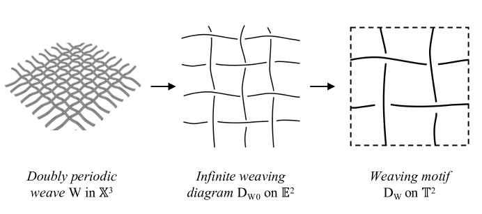
Figure 1. A doubly periodic weave (left), its infinite diagram (center), its quotient link diagram by an integer lattice (right).

In this paper, we first generalize the notion of periodic weaves to the hyperbolic thickened plane. Hence, the corresponding infinite diagrams lie on the Poincare disk. The definition of weaving motifs as link diagrams on higher genus surfaces is obtained through the quotient of a periodic diagram by a discrete group generated by translations. It follows that this approach differs from the classical theory of links embedded in a thickened surface. More precisely, the periodicity in the universal cover is not encoded in the definition of equivalence classes of classic links, which thus fails to classify weaves. This notion has been discussed in [10] for the Euclidean case and is extended to the hyperbolic plane in Section 2.

In the history of knot theory, much attention has been paid to classify alternating links. An alternating link is a link that admits at least one diagram whose crossings alternate between over and under as one travels around each component [19]. In the late nineteenth century, P.G. Tait [21] stated several famous conjectures on alternating links that remained unproven for a century, until the discovery of the Jones polynomial. The first conjecture classifies alternating links by their minimal number of crossings. It was demonstrated independently for links in $\mathbb{S}^{3}$ by M.B Thistlethwaite [23], K. Murasugi [17], and L.H. Kauffman [11]. More recently, T. Fleming et al. [1], [6], and H.U. Boden et al. [2], [3] generalized it for links in thickened surfaces. Tait’s second conjecture for alternating links follows from the first one and classifies oriented diagrams by their writhe. The writhe of a link is the sum of the signs of all the crossings, where each crossing is assigned a sign $\pm 1$. This second conjecture was originally proven independently by M.B Thistlethwaite [23] and K. Murasugi [18] for the case of links in $\mathbb{S}^{3}$. It has also been extended to links in a thickened surface by H.U. Boden et al. in [2] and [3].

The notion of alternating links also appears at the level of weaves. In particular, an alternating periodic weave is a weave that admits at least an alternating weaving motif. One can thus generalize Tait’s conjectures to periodic weaves in a thickened plane. The main purpose of this paper is to prove these conjectures for alternating weaving motifs on a thickened surface. Here, the periodicity in the universal cover must be taken into consideration at the diagrammatic level, which differs from the classical case. More precisely, we will first prove the following.

Theorem 1.1.

(Tait’s First Conjecture for Alternating Weaving Motifs) A minimal reduced alternating weaving motif is a minimum diagram of its alternating periodic weave.

As mentioned earlier, three different proofs of the first conjecture has been stated for classic links in $\mathbb{S}^{3}$. We will follow the combinatorial approach of [11] to prove Theorem. 1.1, where all steps are adapted for alternating weaves. We do that by first defining what we call a reduced weaving motif, which plays the role of a reduced diagram in the original proof. Intuitively, a reduced motif can be thought of as a diagram where no crossing can be removed, as detailed in Definition. 2.10. We then extend the bracket-type polynomial defined in [9] for weaving motifs on higher genus surfaces. Note that it is important to emphasize on the fact that periodic weaves cannot be classified as classic links embedded in a thickened surface. Hence, the original proof fails for the case of periodic weaves in the thickened plane and the aim of this paper is to fill that gap. An important remark is now needed. By considering different point lattices, one may obtain non-equivalent weaving motifs that represent the same weave. For example in Fig. 2, the blue, green and red diagrams are weaving motifs which lift to the same weave in the universal cover. Moreover, for a given fixed integer lattice, one can select two unit cells randomly (mid of Fig. 2) which are not considered equivalent in the sense of the classical theory. As a notable consequence, note that two non-equivalent torus knots lift to the same periodic structure in the Euclidean thickened plane. Therefore, we should consider that the classification of periodic weaves depends on the choice of the lattice. In this paper, we are in particular interested in classifying weaves by invariants depending on the number of crossings. This leads to the need of introducing the notion of minimal lattice, defined in Section 2.1, that generates what we should call minimal motifs. Then, within an equivalence class of minimal weaving motifs, each diagram that contains the minimal number of crossings, namely the crossing number, is said to be minimum. Note that a minimum diagram is always minimal by definition but the converse may not hold. For example, in Fig. 2, the red weaving motif is a minimal and minimum motif for the corresponding periodic weave. Besides, one can also consider that up to isotopy, this red motif is contained in the green and blue motifs. We will thus introduce the notion of scale-equivalence, to encode that the lifts to the universal cover of all these distinct link diagrams define the same periodic weave in a thickened plane.

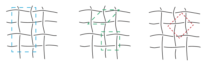
Figure 2. Different generating cells for the same doubly periodic biaxial alternating weave. On the left, the number of crossings is 8 for the blue diagram. In the center, two equivalent green diagrams with 4 crossings. On the right, a red minimal diagram with 2 crossings.

We now naturally consider the generalization of Tait’s second conjecture for periodic weaves. In particular, we will prove the following.

Theorem 1.2.

(Tait’s Second Conjecture for weaves) Any two connected minimal reduced alternating diagrams of an oriented doubly periodic weave have the same writhe.

The proof of Theorem. 1.2 follows the strategy of the one from R. Strong [20] for classic links embedded in $\mathbb{S}^{3}$. The main difference when generalizing this results to periodic weaves is also the consideration of the choice of periodic lattices as well as the fact that the quotient of weaving thread, which is a unknotted open curve in the plane, can be a knotted closed curve on the torus.

This paper is organized as follows. In Section 2, we introduce definitions of periodic weaves and their diagrams. In Section 3, we first recall necessary results on the bracket polynomial for weaving motifs on a torus and we generalize this polynomial to motifs on higher genus surfaces using Teichmüller theory. In Section 4, we present the proof of the main theorem of this paper, that is Tait’s first conjecture for weaves. Finally, in Section 5, we expose the proof of Tait’s second conjecture for weaves, with the use of the proof of the first conjecture.

2. Periodic weaves and their corresponding links in thickened surfaces

2.1. Doubly periodic weaves and links in a thickened torus

Let $L$ be a link in the thickened torus $T^{2}\times I$ whose components are essential closed curves. Let $u,v$ be the basis of the Euclidean plane $\mathbb{E}^{2}$ such that the covering map

$$\rho:\mathbb{E}^{2}\rightarrow{}\mathrm{T}^{2}$$

sends $u$ and $v$ to the meridian $\alpha$ and the longitude $\beta$ of $\mathrm{T}^{2}$, respectively. The link $L$ is assumed to be in general position and we consider its regular projection on the surface of $T^{2}$. If $\omega$ is an essential curve on $T^{2}$, then its lift by $\rho$ is a set of infinite open curves related by a planar translation on $\mathbb{E}^{2}$, called threads. We say that two such threads belong to the same set of threads and run along parallel axes of direction. Moreover, if two essential closed curves $\omega_{1}$ and $\omega_{2}$ on $T^{2}$ are such that $\rho\circ\omega_{1}=\rho\circ\omega_{2}$, up to isotopy, then they are also said to be in the same set of threads, as do their lifts.

Next, if a link component $\omega$ on $T^{2}$ admits a self-crossing, then we are interested in distinguishing the cases when this crossing vanishes in the universal cover. In particular, if a thread has no self-crossing in the universal cover, we say that it is unknotted. We refer to [22] for the details of the following arguments. Let $\omega$ be an essential closed curve on $T^{2}$ and let $p$ be a self-intersection point of $\omega$. Then, $p$ divides $\omega$ into two closed curves, both being seen as homology cycles. By walking on these loops starting from $p$, one will return to $p$ from the left of the starting direction and the other from the right, both being denoted by $\omega_{p}$ and $\omega^{\prime}p$, respectively. We call $\omega_{p}$ and $\omega^{\prime}_{p}$ the divided curves of $\omega$ for $p$. Next, considering $T^{2}=\mathbb{E}^{2}\setminus\mathbb{Z}^{2}$, we define the restriction

$$\Omega:[0,1]\mapsto\mathbb{E}^{2}$$

of the lift $\omega\circ\rho$ to $\mathbb{E}^{2}$, such that $\Omega(0)=(0,0)$. Since $\omega$ is essential on $T^{2}$, $\omega\neq 0$ in $H_{1}(T^{2},\mathbb{Z})$. Thus, $\Omega(1)\neq\Omega(0)$. Moreover, if $\omega_{p}\neq 0$ and $\omega^{\prime}_{p}\neq 0$ in $H_{1}(T^{2},\mathbb{Z})$, then the intersection point $p$ vanishes on the lift $\Omega$. Otherwise, if a divided curve $\omega_{p}$ or $\omega^{\prime}_{p}$ is null-homologous in $H_{1}(T^{2},\mathbb{Z})$, then it lifts to a closed component on $\mathbb{E}^{2}$ since $H_{1}(T^{2},\mathbb{Z})$ is isomorphic to the fundamental group of the torus with basepoint $p$, and thus the intersection point is also lifted.

Definition 2.1.

Let $L_{W}$ be a link in $T^{2}\times I$ with meridian $\alpha$ and longitude $\beta$ satisfying the two following conditions,

1. each of its components is an essential closed curve that lifts to an unknotted thread,

2. its components can be partitioned into $N\geq 2$ sets of threads.

Then, the lift of $L_{W}$ under $\rho$ is called a doubly periodic weave, denoted by $W$, with $N$ sets of threads. Moreover, the projection of $L_{W}$ onto $\mathrm{T}^{2}$ is called a link diagram of $L_{W}$, denoted by $D_{W}$, and the lift $W_{0}$ of $D_{W}$ under $\rho$ is called a doubly periodic diagram.

Considering the above notations, the set of points $\Lambda(u,v)=\{xu+yv/x,y\in\mathbb{Z}\}$ generated by the basis $u,v$ of $\mathbb{E}^{2}$ defines a periodic lattice of unit parallelograms. In particular, each of these parallelograms defines the boundary of a flat generating cell of $D$, considering the identification space of the torus. In other words, a generating cell is the quotient of $W_{0}$ by $\Lambda(u,v)$. However, it is well-known that different bases of $\mathbb{E}^{2}$ can generate equivalent point lattices. More specifically,

$$\Lambda(u,v)\simeq\Lambda^{\prime}(u^{\prime},v^{\prime})\,\textit{ if and only if }\,\begin{pmatrix}u^{\prime}\\ v^{\prime}\end{pmatrix}=\begin{pmatrix}a&b\\ c&d\end{pmatrix}\times\begin{pmatrix}u\\ v\end{pmatrix}\textit{ , where }\mid{ad-bc}\mid=\pm 1$$

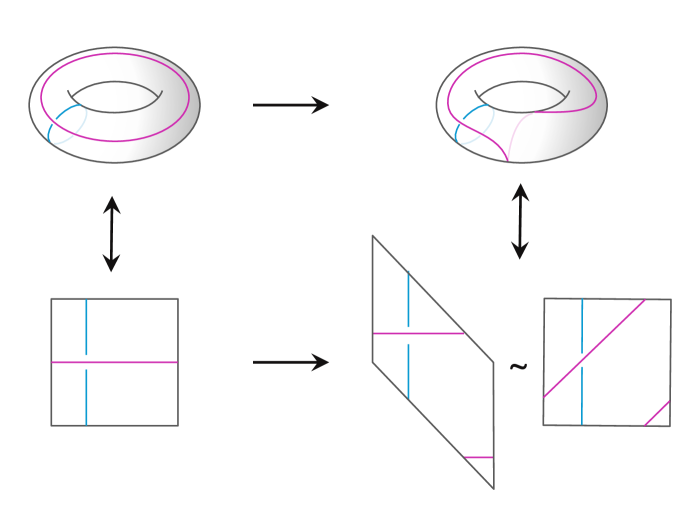
Figure 3. A Dehn twist visualized on a flat torus.

This implies that different generating cells, seen as link diagrams on a flat torus, may lift to the same doubly periodic weave. This leads to the following definition.

Definition 2.2.

Every link diagram on $T^{2}$ that lifts to the same doubly periodic weave is called a weaving motif of the weave.

It is well-known that this equivalence of point lattices can be translated at the level of the torus. Considering linear orientation-preserving homeomorphism of $\mathbb{E}^{2}$, namely matrices of $SL(2,\mathbb{Z})$, the equivalence of generating cells that differ by a change of basis of $\mathbb{E}^{2}$ can be translated into Dehn twists of $T^{2}$, see Fig. 3 for illustration and [5], [10] for details. It follows that for a fixed point lattice, the equivalence of doubly periodic weaves can be described combinatorially by the following.

Proposition 2.3.

(Generalized Reidemeister Theorem for Fixed Point Lattices in $\mathbb{E}^{2}$ [10]) Two doubly periodic weaves in $\mathbb{E}^{2}\times I$ are isotopic for equivalent point lattices if and only if their corresponding weaving motifs can be obtained from each other by a finite sequence of Reidemeister moves $R_{1}$, $R_{2}$, and $R_{3}$, torus isotopies and Dehn twists.

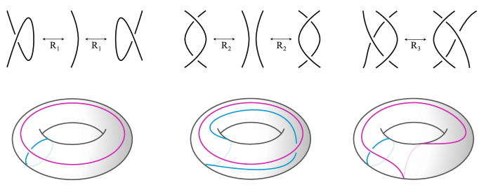
Figure 4. On the top, the three classical Reidemeister moves. On the bottom, a torus with a meridian and a longitude curves (left), its longitudinal twist (middle) and its meridional twist (right)

However, this notion of equivalence is not strong enough to capture non-equivalent point lattices associated with weaving motifs that lift to equivalent periodic weaving diagrams, as illustrated in Fig. 2. Consider for example,

$$\Lambda(u,v)=\{xu+yv/x,y\in\mathbb{Z}\}\,\textit{ and }\,\Lambda^{\prime}(u^{\prime},v^{\prime})=\{xu^{\prime}+yv^{\prime}/x,y\in\mathbb{Z}\}$$

be two non-equivalent lattices associated to the same doubly periodic weaving diagram $W_{0}$ and let $k_{u}$ and $k_{v}$ be two positive integers satisfying,

$$u^{\prime}=k_{u}\times u\,\textit{ and }\,v^{\prime}=k_{v}\times v.$$

It follows that $\Lambda$ is contained in $\Lambda^{\prime}$ ($\Lambda\subseteq\Lambda^{\prime}$). Note now that any two weaving motifs $D_{W}=W_{0}\setminus\Lambda$ and $D^{\prime}_{W}=W_{0}\setminus\Lambda^{\prime}$ are not necessarily equivalent by Proposition 2.3, althought they both lift to the same periodic weaving diagram in the plane. This leads to the definition of the notion of scale-equivalence between weaving motifs. Note that this inclusion relation guarantees the existence of a minimal lattice, denoted by $\Lambda_{min}=\Lambda(u_{min},v_{min})$, such that for any periodic lattice $\Lambda(u,v)$ of $W$, $\Lambda_{min}\subseteq\Lambda(u,v)$.

Definition 2.4.

Let $W_{0}$ be a doubly periodic weaving diagram and let $\Lambda_{1}$ and $\Lambda_{2}$ be two non-equivalent point lattices such that $\Lambda_{1}\subset\Lambda_{2}$. Moreover, let $D_{W_{1}}=W_{0}\setminus\Lambda_{1}$ and $D_{W_{2}}=W_{0}\setminus\Lambda_{2}$ be two weaving motifs of $W_{0}$. Then, $D_{W_{1}}$ and $D_{W_{2}}$ are said to be scale-equivalent if there exists a weaving motif $D^{\prime}_{W_{1}}$ defined as adjacent copies of $D_{W_{1}}$ such that $D^{\prime}_{W_{1}}=W_{0}\setminus\Lambda_{2}$ is a weaving motif of $W_{0}$ for $\Lambda_{2}$.

From now on, we will consider equivalence of doubly periodic weaves by extending the notion of isotopy to scale-equivalence.

Definition 2.5.

Let $W_{1}$ and $W_{2}$ be two doubly periodic weaves with weaving diagrams $W_{01}$ and $W_{02}$ and let $\Lambda_{1}\subset\Lambda_{2}$ be two non-equivalent point lattices such that for $i\in\{1,2\}$, $D_{W_{i}}=W_{0i}\setminus\Lambda_{i}$ is a weaving motif of $W_{i}$. Then, $W_{1}$ and $W_{2}$ are equivalent if the two following conditions are satisfied,

• $D_{W_{1}}$ and $D_{W_{2}}$ are scale-equivalent with $D_{W_{1}}\subset D^{\prime}_{W_{1}}$ and $D^{\prime}_{W_{1}}=W_{01}\setminus\Lambda_{2}$,

• $D^{\prime}_{W_{1}}$ and $D_{W_{2}}$ are related by a finite sequence of Reidemeister moves $R_{1}$, $R_{2}$, and $R_{3}$, torus isotopies and Dehn twists.
  

2.2. Generalization to hyperbolic weaves and diagrams on higher genus surfaces

The study of weaving motifs on the torus encourages a generalization to higher genus surfaces. This implies a definition of periodic weaving diagrams on the hyperbolic plane $\mathbb{H}^{2}$. However, note that the notion of parallel directions considered to define our sets of threads in $\mathbb{E}^{2}$ cannot be extended to $\mathbb{H}^{2}$. We thus restrict our definition of hyperbolic weaves to the cases where their regular projections are isotopic to quadrivalent kaleidoscopic tilings of $\mathbb{H}^{2}$. A kaleidoscopic tiling is constructed by applying repetitively reflection symmetries along the sides of a given hyperbolic convex polygon (Fig. 5). We will use the Poincare disk representation of $\mathbb{H}^{2}$ and refer to [4] for more details on hyperbolic kaleidoscopic tilings.

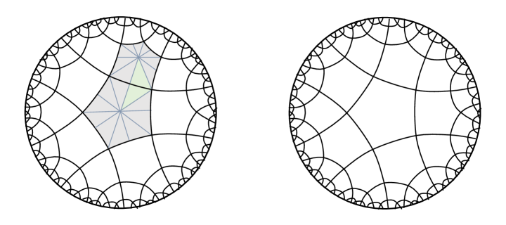
Figure 5. Example of kaleidoscopic tiling of the hyperbolic plane.

Definition 2.6.

Let $P$ be the generating convex polygon of a quadrivalent kaleidoscopic tiling $\mathcal{T}$ of $\mathbb{H}^{2}$ and let $N\geq 3$ be the number of edges of $P$. If $N$ is odd, then each edge is assigned a different axis of direction. Otherwise, each pair of opposite edges of $P$ are given the same direction.

Remark 2.7.

Since reflection symmetries preserves the axis of direction by construction, the notion of sets of threads in $\mathbb{H}^{2}$ is defined in a coherent way that generalizes the definition in $\mathbb{E}^{2}$, as shown in Fig. 6.

Therefore, by specifying each vertex of a hyperbolic kaleidoscopic tilings with an over or under crossing information, we introduce a new class of periodic weaves in $\mathbb{H}^{2}\times I$. Note that most of the definitions stated in [7] may follow naturally here. Two examples of periodic hyperbolic weaving diagrams are illustrated in Fig. 6.

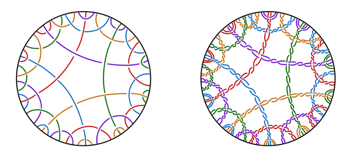
Figure 6. Example of sets of threads for a weaving diagram of the hyperbolic plane.

It follows that a hyperbolic weaving motif can be defined as a link diagram on a surface $S_{g}$ of genus $g\geq 2$. In particular, this results from the pairwise identification of the sides of a generating cell, defined as the quotient of a periodic weaving diagram of $\mathbb{H}^{2}$ by a discrete lattice. More precisely, a flat weaving motif is a set of simple open arcs and crossings on a hyperbolic polygon. Note that this polygon can be chosen in infinitely many ways, the easiest being a regular $4g$-gons of $\mathbb{H}^{2}$ (Fig. 7). This leads to a generalization of the theory of weaving motifs on a torus to motifs on higher genus surfaces. We consider any closed orientable surface $S_{g}$ of genus $g\geq 2$ with generating loops $\alpha_{1},\cdots,\alpha_{g}$ and $\beta_{1},\cdots,\beta_{g}$. These loops define homotopy classes through a common base point on $S_{g}$ and map to a basis of $\mathbb{H}^{2}$.

Definition 2.8.

Let $L_{W}$ be a link in $S_{g}\times I$ of genus $g\geq 2$ with generating loops $\alpha_{1},\cdots,\alpha_{g}$ and $\beta_{1},\cdots,\beta_{g}$, satisfying the two following conditions,

1. each of its components is an essential closed curve that lifts to an unknotted thread,

2. its components can be partitioned into $N\geq 2$ sets of threads.

Then, the lift of $L_{W}$ under the covering map $\rho^{\prime}:\mathbb{H}^{2}\times I\rightarrow{}S_{g}\times I$ is called a hyperbolic periodic weave $W$ with $N$ sets of threads. Moreover, the projection of $L_{W}$ onto $S_{g}$ is called a link diagram of $L_{W}$, denoted by $D_{W}$, and the lift $W_{0}$ of $D_{W}$ under $\rho^{\prime}$ is called a hyperbolic weaving diagram.

Now, to generalize the notion of equivalent weaving motifs on the torus to higher genus surfaces, one needs to consider the Teichmüller space of a surface $S_{g}$ of genus $g\geq 2$, and its mapping class group. We refer to [5] for a complete study of mapping class groups. First, start from any hyperbolic motif, whose flat boundary is a geodesic hyperbolic $4g$-gon on $\mathbb{H}^{2}$, meaning a polygon such that the sum of its interior angles is equal to $2\pi$. Then, label its edges such that they can be identified pairwise, which results in a closed marked hyperbolic surface $S_{g}$ of genus $g\geq 2$, as illustrated in Fig. 7. Such a polygon is called a $S_{g}$-tile and the Teichmüller space of the corresponding surface $S_{g}$ can be seen as the space of marked surfaces homeomorphic to it. Moreover, it is well-known that the Teichmüller space of $S_{g}$ is in bijection with the set of equivalence classes of hyperbolic $S_{g}$-tiles. Note that two $S_{g}$-tiles are said to be equivalent if they differ by a marked, orientation-preserving isometry and by pushing the basepoint, which is the point on the surface where all the vertices of a $S_{g}$-tile meet after gluing. The details of this bijection are given in [5].

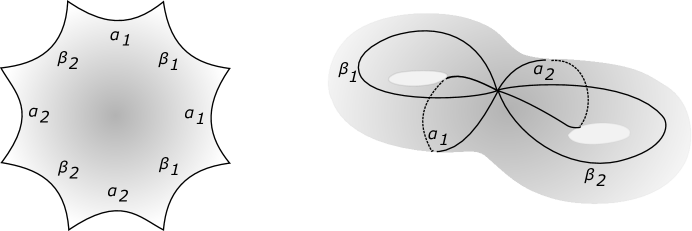
Figure 7. A regular $S_{2}$-tile and its corresponding marked hyperbolic surface.

Now, to prove the existence and relation between infinitely many $S_{g}$-tiles, we start from an arbitrary point in $\mathrm{Teich}(S_{g})$, the Teichmüller space of $S_{g}$, which represents the equivalence class of a marked surface $S_{g}$ of genus $g$. From the above bijection, $\mathrm{Teich}(S_{g})$ corresponds to the equivalence class of isometric $S_{g}$-tiles, each corresponding to a unique point in $\mathrm{Teich}(S_{g})$. Thus, if there exists a non-isometric $S_{g}$-tile that can be taken as a unit cell of the same hyperbolic weaving diagram, then it corresponds to a different marked surface and is not isometric to the original $S_{g}$-tile. However, there exists a relation between these different markings of $S_{g}$, characterized by its mapping class group $MCG(S_{g})$, whose simplest infinite-order elements are known to be Dehn twists, as in the torus case. Indeed, given any marked surface $S_{g}$ of genus $g$ in $\mathrm{Teich}(S_{g})$, the marking can be changed by the action of any finite sequence of Dehn twists, which generates non-isometric corresponding $S_{g}$-tiles. Thus, this proves the existence of infinitely many weaving motifs for any periodic hyperbolic weaving diagram on $\mathbb{H}^{2}$. In other words, for any given periodic weaving diagram and a corresponding point lattice, every weaving motifs can be obtained from an arbitrarily chosen one by a finite sequence of Dehn twists of $S_{g}$ along its generating loop, which are extensions of the meridians and longitudes of a torus [15]. Therefore, to define equivalence class of periodic weaves in terms of ambient isotopy in the thickened hyperbolic plane, we can use the above arguments to encode the periodicity and the relation between all possible unit cells for a given lattice, which generalizes Definition 2.5.

Theorem 2.9.

Let $W_{1}$ and $W_{2}$ be two periodic hyperbolic weaves with weaving diagrams $W_{01}$ and $W_{02}$ in $\mathbb{H}^{2}$ and let $\Lambda_{1}\subset\Lambda_{2}$ be two non-equivalent point lattices such that for $i\in\{1,2\}$, $D_{W_{i}}=W_{0i}\setminus\Lambda_{i}$ is a weaving motif of $W_{i}$ on $S_{g}$. Then, $W_{1}$ and $W_{2}$ are equivalent if the two following conditions are satisfied,

• $D_{W_{1}}$ and $D_{W_{2}}$ are scale-equivalent with $D_{W_{1}}\subset D^{\prime}_{W_{1}}$ and $D^{\prime}_{W_{1}}=W_{01}\setminus\Lambda_{2}$,

• $D^{\prime}_{W_{1}}$ and $D_{W_{2}}$ are related by a finite sequence of Reidemeister moves $R_{1}$, $R_{2}$, and $R_{3}$, isotopies and Dehn twists of $S_{g}$.
  

2.3. Some particular weaving diagrams

Many definitions from classical knot theory [11, 19] can be naturally extended for weaving diagrams. In particular, a weave $\mathrm{W}$, or any associated weaving diagram or motif, is said to be alternating if its crossings alternate cyclically between undercrossings and overcrossings, as one travels along each of its components (see Fig. 8). However, the notion of reduced diagrams does not follow directly from links in the thickened surfaces but takes into account the universal cover. More specifically, we have the following.

Definition 2.10.

A weaving motif $D_{\mathrm{W}}$ in $S_{g}$, with $g\geq 1$, is said to be reduced if its lift to the universal cover $\mathbb{X}^{2}=\mathbb{E}^{2}$ or $\mathbb{H}^{2}$ does not contain a nugatory crossing. A nugatory crossing is a crossing in the diagram so that two of the four local regions at the crossing are part of the same region in the associated infinite diagram.

Moreover, at the level of the torus, any crossing $c$ of a weaving motif $D_{\mathrm{W}}$ is called proper if the four regions around $c$ delimited by the projection of the threads are all distinct. When every crossing of $D_{\mathrm{W}}$ is proper, $D_{\mathrm{W}}$ is said to be proper (see Fig. 8).

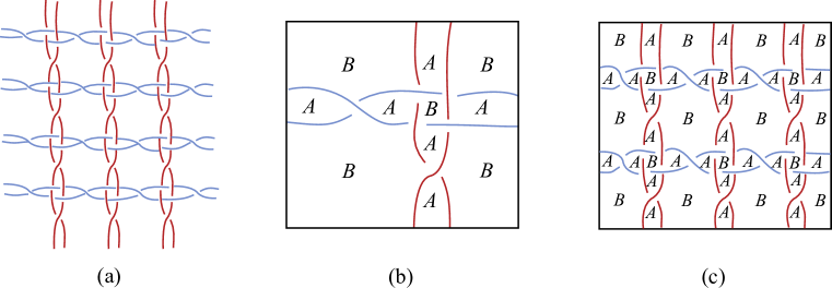
Figure 8. A periodic reduced (without nugatory crossing) planar diagram (a), a reduced improper weaving motif (b), and a reduced proper weaving motif (c).

Note that an equivalent definition of reduced diagram can be stated using the point lattice inclusion defined above.

Definition 2.11.

A weaving motif $D_{W}$ for a point lattice $\Lambda$ is said to be reduced if one of the two following conditions is satisfied,

• all its crossings are proper,

• for each improper crossing $c$, there exists a point lattice $\Lambda^{\prime}$ such that $\Lambda\subset\Lambda^{\prime}$ and for which $c$ is proper in $D^{\prime}_{W}$, where $D^{\prime}_{W}$ is the weaving motif constructed by gluing a copy of $D_{W}$ to each of its boundary sides by translation.

Remark 2.12.

Recently, in [2], a different definition of reduced diagram for classic links on a thickened surface has been stated and could also apply here.

3. The Bracket Polynomial of Periodic Weaves

3.1. A Kauffman-type weaving invariant

This section recalls results from [9] and [10], and extends the definition of the bracket polynomial of a weaving motif on a torus to any surface $S_{g}$ of genus $g\geq 1$.

Definition 3.1.

Let $D_{\mathrm{W}}$ be a weaving motif on a surface $S_{g}$ of genus $g\geq 1$, and let $\langle D_{\mathrm{W}}\rangle$ be the element of the ring $\mathbb{Z}[A,B,d]$ defined recursively by the following identities,

1. $\langle O\rangle=1$, with $O$ a null-homotopic simple closed curve on $D_{\mathrm{W}}$.

2. $\langle D_{\mathrm{W}}\cup O\rangle=d\langle D_{\mathrm{W}}\rangle$, when adding an isolated circle $O$ to a diagram $D_{\mathrm{W}}$.

3. $\langle$ $\rangle$ = $A$$\langle$ $\rangle$$+$ $B$$\langle$ $\rangle$, for diagrams that differ locally around a single crossing.

This last relation is called the skein relation and $\langle D_{\mathrm{W}}\rangle$ denotes the bracket polynomial.

This polynomial is known to be well defined on classic link diagrams and can be generalized to periodic weaves. Let $D_{W}$ be any weaving motif of a periodic weave of $\mathbb{X}^{2}=\mathbb{E}^{2}$ or $\mathbb{H}^{2}$. Then, every crossing of $D_{\mathrm{W}}$ can be smoothed via an operation of type $A$ or $B$, as illustrated in Fig. 9. The overall operations can be expressed as a state $S$ of $D_{\mathrm{W}}$, defined as a sequence of symbols $A$ and $B$ of length $C$, where $C$ is the number of crossings of $D_{\mathrm{W}}$,

$$S=ABAABB…ABBA.$$

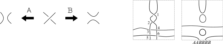
Figure 9. On the left, the two types of splitting. On the right, an example of a state $S=AABBBB$ of a weaving motif.

It is well-known for links in $\mathbb{S}^{3}$ that a diagram $D_{S}$ in a state $S$ is a disjoint union of $c_{S}$ null-homotopic simple closed curves. It follows from Definition 3.1(2) that,

$$\langle D_{S}\rangle=d\,^{c_{S-1}}.$$

Moreover, if $i$ is the number of splits of type $A$ and $j$ the number of splits of type $B$, then the total contribution of the state $S$ to the bracket polynomial is given by applying the skein relation recursively,

$$P_{S}=\langle D_{S}/S\rangle\langle D_{S}\rangle=A^{i}B\,^{j}d\,^{c_{S-1}}.$$

However, recall that a state of a weaving motif $D_{\mathrm{W}}$ may contain essential simple closed curves, as in the case of any link diagram on a surface $S_{g}$ of genus $g\geq 1$. Such a set is called a winding in [9] and is denoted by $(m,n)_{S}$ for $g=1$, where $m$ and $n$ are the number of intersections of the winding with a torus meridian and longitude, respectively. For example, in the case of the state diagram of Fig. 9 (right), $(AABBBB)$, we have $(m,n)_{S}=(0,2)_{S}$.

For the general case of $g\geq 1$, a winding is denoted by,

$$(m_{1},\cdots,m_{g},n_{1},\cdots,n_{g})_{S},$$

where $m_{1},\cdots,m_{g},n_{1},\cdots,n_{g}$ are the number of intersections of the winding with the generating loops $\alpha_{1},\cdots,\alpha_{g},\beta_{1},\cdots,\beta_{g}$ of the surface $S_{g}$ respectively, see Fig. 7 and [15] for more details.

Recall that by definition, windings also encode the periodicity of weaves in the universal cover, which is not considered for classic links in a thickened surface, as in [1, 3, 2, 6]. We can thus generalize the value of the bracket polynomial of a winding defined for $g=1$ in [9], with respect to Definition 3.1,

$$\langle(m_{1},\cdots,m_{g},n_{1},\cdots,n_{g})_{S}\rangle\ =\ (m_{1},\cdots,m_{g},n_{1},\cdots,n_{g})_{S},\mbox{ for every }g\geq 1.$$

Therefore, following the above reasoning, the bracket polynomial of a weaving motif is well-defined.

Proposition 3.2.

The bracket polynomial $\langle D_{\mathrm{W}}\rangle$ of a weaving motif $D_{\mathrm{W}}$ on a surface $S_{g}$ of genus $g\geq 1$ is uniquely determined by the identities (1), (2), (3) of Definition 3.1, and is expressed by summation over all states of the diagram,

$$\langle D_{\mathrm{W}}\rangle=\sum_{S}A^{i}B\,^{j}d\,^{c_{S}}(m_{1},\cdots,m_{g},n_{1},\cdots,n_{g})_{S}.$$ (3.1)

As for links in $\mathbb{S}^{3}$, the bracket polynomial of a weaving motif is proven to be invariant under the Reidemeister moves following the same approach of Lemma 2.3 in [11].

Lemma 3.3.

If the three diagrams represent the same weaving motif except in the area indicated, we have $\langle$ $\rangle$ = $AB$$\langle$ $\rangle$ $+$ $(ABd+A^{2}+B^{2})$$\langle$ $\rangle$.

Thus, the bracket is invariant for the Reidemeister move $R_{2}$ for all diagrams if

$$AB=1\mbox{ and }d=-A^{2}-A^{-2}.$$

Moreover, this implies also the invariance of the bracket for the Reidemeister move $R_{3}$, which concludes the invariance by regular isotopy.

Lemma 3.4.

The bracket invariance for the Reidemeister move $R_{2}$ implies the bracket invariance for the Reidemeister move $R_{3}$. Thus, the bracket polynomial is an invariant of regular isotopy for periodic weaves for a fixed point lattice.

Finally, to prove the invariance uner the Reidemeister move $R_{1}$, we use the following proposition that provides an identity for $R_{1}$, as in [11].

Proposition 3.5.

If $AB=1$ and $d=-A^{2}-A^{-2}$, then, for the Reidemeister move $R_{1}$, we have

$$\left\{\begin{array}[]{ll}\langle\ \raisebox{-3.0pt}{\includegraphics[scale={0.4}]{351.pdf}}\ \rangle=(-A^{3})\langle\ \raisebox{1.0pt}{\includegraphics[scale={0.4}]{353.pdf}}\ \rangle,\\ {}\\ \langle\ \raisebox{-3.0pt}{\includegraphics[scale={0.38}]{352.pdf}}\ \rangle=(-A^{-3})\langle\ \raisebox{1.0pt}{\includegraphics[scale={0.4}]{353.pdf}}\ \rangle.\\ \end{array}\right.$$

The strategy is to use the writhe $w_{r}(D_{\mathrm{W}})$ of a weaving motif $D_{\mathrm{W}}$, which is the sum of the signs of all the crossings, where each crossing is given a sign $\pm 1$, as in Fig. 10.

Figure 10. Sign convention.

Any weaving motif $D_{\mathrm{W}}$ consists of $T$ essential closed curve components, each denoted by $t_{i}$, that can be oriented in an arbitrary way. We call $D^{i}_{\mathrm{W}}$ the part of the diagram $D_{\mathrm{W}}$ that corresponds to the component $t_{i}$. Then we have in $D_{\mathrm{W}}$,

$$w_{r}(D_{\mathrm{W}})=\sum_{i=1}^{T}w_{r}(D^{i}_{\mathrm{W}}).$$ (3.2)

We can now define a polynomial constructed from the bracket. For every $g\geq 1$, we set

$$f(D_{\mathrm{W}}) =(-A)^{-3w_{r}(D_{\mathrm{W}})}\langle D_{\mathrm{W}}\rangle,$$ (3.3)

$$=(-A)^{-3w_{r}(D_{\mathrm{W}})}\Bigl{(}\sum_{S}A^{i-j}(-A^{2}–A^{-2})^{c_{S}}(m_{1},\cdots,m_{g},n_{1},\cdots,n_{g})_{S}\Bigr{)}.$$

Theorem 3.6.

The polynomial $f(D_{\mathrm{W}})\in\mathbb{Z}[A]$ defined above is an ambient isotopic invariant for oriented weaves under a fixed point lattice.

Proof.

From Lemma 3.4, we already have the invariance of $f(D_{\mathrm{W}})$ for the Reidemeister moves $R_{2}$ and $R_{3}$. Then, by combining the behavior of the writhe defined above under the Reidemeister move $R_{1}$ with the previous relation of the bracket for $R_{1}$ in Proposition 3.5, it follows that $f(D_{\mathrm{W}})$ is invariant under $R_{1}$ type moves. Thus, $f(D_{\mathrm{W}})$ is invariant under all three moves, and is therefore an invariant of ambient isotopy for the chosen lattice. $\Box$

Nevertheless, this polynomial still depends on the choice of the unit cell for the chosen point lattice, since the multipliers $(m_{1},\cdots,m_{g},n_{1},\cdots,n_{g})_{S}$ describing the windings depend on the Dehn twists of the surface $S_{g}$. As seen earlier, to have a weaving invariant for a fixed lattice, we also need the invariance of the polynomial under Dehn twists of $S_{g}$. Once again, the particular case of the torus is described in [9] and is generalized below to $g\geq 1$.

Theorem 3.7.

The polynomial $f(D_{\mathrm{W}})$, when $(m_{1},\cdots,m_{g},n_{1},\cdots,n_{g})_{S}$ is in a canonical form for each state $S$, defines a Kauffman-type weaving invariant for a fixed point lattice.

Proof.

To construct an invariant independent of the Dehn twists of $S_{g}$, a possibility is to define a canonical form for the set $\{v_{S}\}$ $=$ $\bigl{\{}(m_{1},\cdots,m_{g},n_{1},\cdots,n_{g})_{S}\bigr{\}}$ of windings for every state $S$. Indeed, since this set $\{v_{S}\}$ depends on the twists of $S_{g}$, one must transform it into the canonical form to make it invariant. The Dehn-Lickorish Theorem states that it is sufficient to select a finite number of Dehn twists to generate the mapping class group $MCG(S_{g})$ of a surface $S_{g}$ of genus $g$. Moreover, since the map $\psi:MCG(S_{g})\to Sp(2g,\mathbb{Z})$ is surjective for $g\geq 1$, it follows that the images of the Dehn twists generate $Sp(2g,\mathbb{Z})$ ([5]). Besides, recall that the determinant of every matrix $U\in Sp(2g,\mathbb{Z})$ is equal to $1$ and that for $g=1$, $Sp(2g,\mathbb{Z})=SL_{2}(\mathbb{Z})$. Thus, following the strategy used in [9], one can represent the transformation of a winding $v_{S}=((m_{1},\cdots,m_{g},n_{1},\cdots,n_{g})_{S}$ by a sequence of Dehn twists of $S_{g}$ as a product of $v_{S}$ by a matrix $U\in Sp(2g,\mathbb{Z})$,

$$v^{\prime}_{S}=v_{S}.U,$$

considering the canonical matrix multiplication on $Sp(2g,\mathbb{Z})$.

To define the canonical form of a set $V=\{v_{S}\}$, we associate a quadratic functional $Q$,

$$Q(V):=\sum_{S}^{N}|v_{S}|^{2}.$$ (3.4)

Thus, a finite sequence of Dehn twists, given by a matrix $U$, converts the set of windings $V=\{v_{S}\}$ to a set $V^{\prime}=\{v^{\prime}_{S}\}$, with $v^{\prime}_{S}=v_{S}.U$ and the value of $Q$ becomes,

$$Q(V^{\prime})=\sum_{s}^{N}|v^{\prime}_{S}|^{2}=\sum_{S}^{N}v_{S}.U.U^{T}.v_{S}^{T}.$$ (3.5)

Then, to construct a canonical form of the windings $V=\{v_{S}\}$, the idea is to find a finite sequence of Dehn twists encoded in $U$ that minimizes the value of $Q$ ([9]),

$$Q(V^{\prime})=\sum_{S}^{N}|v^{\prime}_{S}|^{2}=\sum_{S}^{N}v_{S}.U.U^{T}.v_{S}^{T}\longrightarrow\min,U\in Sp(2g,\mathbb{Z}).$$ (3.6)

This equation always has a unique non-trivial solution $U_{0}$. Indeed, let $M=U.U^{T}$ be a symmetric definite positive matrix. Then, if $x=v_{S}$ and $\phi(x)=x.M.x^{T}$, then $\phi(0)=0$ and for all $x\neq 0$, $\phi(x)>0$. Thus, there exists an orthonormal basis $\{e_{1},\cdots,e_{d}\}$ such that for all $i$ in $\{1,\cdots,d\}$, $e_{i}$ is an eigenvector of $M$. We denote the corresponding eigenvalue $\lambda_{i}$ and we show that $\phi$ is strictly convex.

Let $0<\mu<1$ and consider $\phi\bigl{(}\mu x+(1-\mu)y\bigr{)}$, with $x\neq y$. Then,

$$\phi\bigl{(}\mu x+(1-\mu)y\bigr{)} =\langle\mu x+(1-\mu)y,M(\mu x+(1-\mu)y)\rangle,$$ (3.7)

$$=\langle\sum_{i=1}^{d}\mu x_{i}e_{i}+(1-\mu)y_{i}e_{i},M\sum_{i=1}^{d}\mu x_{i}e_{i}+(1-\mu)y_{i}e_{i}\rangle,$$

$$=\sum_{i=1}^{d}\lambda_{i}\bigl{(}\mu x_{i}+(1-\mu)y_{i}\bigr{)}^{2}.$$

Moreover, $x^{2}$ is strictly convex and for some $i$, $x_{i}\neq y_{i}$, thus,

$$\sum_{i=1}^{d}\lambda_{i}\bigl{(}\mu x_{i}+(1-\mu)y_{i}\bigr{)}^{2}<\sum_{i=1}^{d}\lambda_{i}\bigl{(}\mu x_{i}^{2}+(1-\mu)y_{i}^{2}\bigr{)}.$$ (3.8)

Therefore, since $\phi$ is strictly convex and has a limit at infinity, it has a unique minimum, which concludes our proof. So, for every state $S$, the canonical form of a set of windings $V=\{v_{S}\}$, with the winding as coordinates $v_{S}=(m_{1},\cdots,m_{g},n_{1},\cdots,n_{g})_{S}$ is an invariant and thus, $f(D_{\mathrm{W}})$ too. $\Box$

3.2. The case of alternating weaving diagrams

Now, we study the bracket polynomial for the case of alternating weaves. It is well-known that the degree of a polynomial is the most important aspect of the polynomial as an invariant [18]. The following proposition and its proof follow the strategy of the similar result for classic links in $\mathbb{S}^{3}$, but depend strongly on the definition of reduced and proper diagrams stated in Section 2.3.

Proposition 3.8.

Let $D_{\mathrm{W}}$ be an alternating reduced weaving motif colored so that all the regions labeled $A$ are white and all the regions labeled $B$ are black. Let $\mathit{C}$ be the number of crossings, $W$ be the number of white regions and $B$ be the number of black ones. Then,

$$\max\mathrm{deg}(\langle D_{\mathrm{W}}\rangle) =\mathit{C}+2W,$$ (3.9)

$$\min\mathrm{deg}(\langle D_{\mathrm{W}}\rangle) =-\mathit{C}-2B,$$

with $\max\mathrm{deg}(P)$ and $\min\mathrm{deg}(P)$ are respectively the maximal and the minimal degree of any polynomial $P$ in $\mathbb{Z}[A,B,d]$.

Proof.

Since $D_{\mathrm{W}}$ is alternating, it admits a canonical checkerboard coloring by definition, which means that two edge-adjacent regions always have different colors. Let $S=S_{A}$ be the state obtained by splitting every crossing in the diagram $D_{\mathrm{W}}$ in the $A$-direction. Then we have $\langle D_{\mathrm{W}}/S\rangle=A^{\mathit{C}}$, and since the number of components $c_{S}$ is equal to $\mathrm{W}$, thus as seen earlier, the total contribution of the state $S$ to the bracket polynomial is given by,

$$P_{S} =\langle D_{\mathrm{W}}/S\rangle d\,^{c_{S}}(m_{1},\cdots,m_{g},n_{1},\cdots,n_{g})_{S}$$ (3.10)

$$=A^{\mathit{C}}d\,^{W}(m_{1},\cdots,m_{g},n_{1},\cdots,n_{g})_{S},\ g\geq 1.$$

And since $d=-A^{2}-A^{-2}$, then $\max\mathrm{deg}(P_{S})=\mathit{C}+2W$, which is the desired relation.

Now let $S’\neq S_{A}$ be any other state and verify that $\mathrm{deg}(P_{S’})\ngeq\mathrm{deg}(P_{S})$. Then $S’$ can be obtained from $S=S_{A}$ by switching some splittings of $S$. A sequence of states can be defined by $S(0),S(1),\cdots,S(n)$ such that $S=S(0)$, $S’=S(1)$. Thus, for every positive integer $i$, $S(i+1)$ is obtained from $S(i)$ by switching one splitting from type $A$ to type $B$, which then contributes a factor of $A^{-1}$ in the polynomial

$$\langle D_{\mathrm{W}}/S(i+1)\rangle=A^{-2}\langle D_{\mathrm{W}}/S(i)\rangle.$$ (3.11)

We need now to distinguish two cases.

Case 1. The weaving motif $D_{\mathrm{W}}$ is reduced and proper for the fixed point lattice. Then, $c_{S(i+1)}\leq c_{S(i)}-1$, since switching one splitting can change the component number by at most one. Thus, $\max\mathrm{deg}(P_{S(i+1)})\leq\max\mathrm{deg}(P_{S(i)})$. Moreover, let $c$ be the crossing point for which we change the $A$-splice into the $B$-splice from $S(0)$ to $S(1)$. Since $D_{\mathrm{W}}$ is proper, the crossing $c$ is proper. Thus, we can use the following lemma, (Lemma 3.2 in [12]).

Lemma 3.9.

Let $D_{\mathrm{W}}$ be an alternating weaving motif and let $S_{A}$ (resp. $S_{B}$) be the state of $D_{\mathrm{W}}$ obtained from $D_{\mathrm{W}}$ by doing an $A$-splice (resp. $B$-splice) for every crossing. For a crossing $c$ of $D_{\mathrm{W}}$, let $R_{1}(c)$ and $R_{2}(c)$ be the closed regions of $S_{A}$ (or $R’_{1}(c)$ and $R’_{2}(c)$ be the closed regions of $S_{B}$) around $c$. If $c$ is a proper crossing, then

$$R_{1}(c)\neq R_{2}(c)\textit{ and }R’_{1}(c)\neq R’_{2}(c).$$

Proof.

Since $c$ is a proper crossing, the four closed regions of $D_{\mathrm{W}}$ appearing around $c$ are all distinct. Since $D_{\mathrm{W}}$ is alternating, it has a canonical checkerboard coloring and there is a one-to-one correspondence,

$$\bigl{\{}\mbox{the closed regions of $S_{A}$}\bigr{\}}\cup\bigl{\{}\mbox{the closed regions of $S_{B}$}\bigr{\}}\to\bigl{\{}\mbox{the closed regions of $D_{\mathrm{W}}$}\bigr{\}}$$

Then $R_{1}(c),R_{2}(c),R’_{1}(c)\textit{ and }R’_{2}(c)$ correspond to the four distinct closed regions of $D_{\mathrm{W}}$ around $c$. This concludes the proof. $\Box$

Thus, from this lemma, since $S(1)$ is obtained from $S(0)$ by changing an $A$-splice to a $B$-splice at $c$, two distinct regions $R_{1}(c)$ and $R_{2}(c)$ become a single region. Hence $c_{S(1)}=c_{S}-1.$ To conclude, the term of maximal degree in the entire bracket polynomial is contributed by the state $S=S_{A}$, and is not canceled by terms from any other state, so we arrive at

$$\max\mathrm{deg}(\langle D_{\mathrm{W}}\rangle)=\mathit{C}+2W.$$

The proof is similar for,

$$\min\mathrm{deg}(\langle D_{\mathrm{W}}\rangle)\,=-\mathit{C}-2B.$$

Case 2: The weaving motif is reduced but not proper for the fixed lattice. Then, there exists at least one crossing which is not proper. If we change an $A$-splice to a $B$-splice at a crossing $c$ that is proper, then the conclusion is the same as before. Now, if we change an $A$-splice to a $B$-splice at a crossing $c’$ that is not proper, then some white regions would touch both sides of a crossing. In this case, the number of split components does not decrease from $S(0)$ to $S(1)$, $c_{S(1)}=c_{S(0)}.$ But, as seen before, $\langle D_{\mathrm{W}}/S(1)\rangle=A^{-2}\langle D_{\mathrm{W}}/S(0)\rangle$ and there is no isthmus in the diagram, so the number of components either decreases or is constant. Therefore,

$$\max\mathrm{deg}(P_{S(1)})\leq\max\mathrm{deg}(P_{S(0)}).$$ (3.12)

Thus, once again, the term of maximal degree in the entire bracket polynomial is contributed by the state $S=S_{A}$, and is not canceled by terms from any other state and therefore,

$$\max\mathrm{deg}(\langle D_{\mathrm{W}}\rangle)=\mathit{C}+2W.$$

The proof is similar for,

$$\min\mathrm{deg}(\langle D_{\mathrm{W}}\rangle)\,=-\mathit{C}-2B.$$

$\Box$

Now, it is possible to define a relation between the closed regions of $D_{\mathrm{W}}$ and the regions of the diagram after splitting as in Section 3 [12]. Let $S_{A}$ (resp. $S_{B}$) be again the state obtained by splitting every crossing in the diagram in the $A$ (resp. $B$)-direction, and $D_{\mathrm{W}}$ be colored so that all the regions labeled $A$ are white (gray on Fig. 11) and all the regions labeled $B$ are black.

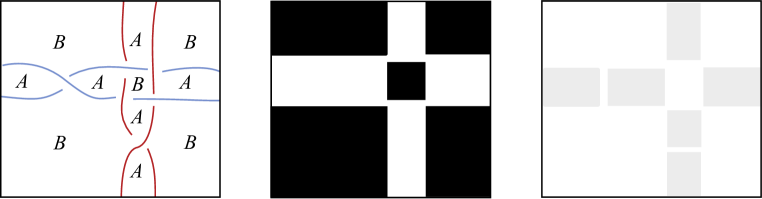
Figure 11. Example of $D_{\mathrm{W}}$ (left), $S_{A}=A\cdots A$ (middle) and $S_{B}=B\cdots B$ (right).

Therefore, we have the following correspondences,

$\bigl{\{}\mbox{the closed regions of $S_{A}$}\bigr{\}}\longrightarrow\bigl{\{}\mbox{the closed regions of $D_{\mathrm{W}}$ in black regions $B$}\bigr{\}}$,

$\bigl{\{}\mbox{the closed regions of $S_{B}$}\bigr{\}}\longrightarrow\bigl{\{}\mbox{the closed regions of $D_{\mathrm{W}}$ in white regions $W$}\bigr{\}}$,

which leads to the following bijection,

$\bigl{\{}\mbox{the closed regions of $S_{A}$}\bigr{\}}\ \cup\ \bigl{\{}\mbox{the closed regions of $S_{B}$}\bigr{\}}\longrightarrow\bigl{\{}\mbox{the closed regions of $D_{\mathrm{W}}$}\bigr{\}}.$

And when considering a diagram on a surface of genus $g\geq 1$, using the Euler characteristic and the fact that such a diagram is quadrivalent, we conclude that,

$$\textit{the number of closed regions of }\,D_{\mathrm{W}}\,\textit{ is equal to }\,\mathit{C}+2-2g,\,\textit{ for every }\,g\geq 1.$$

It is now possible to extend the proof of Theorem 2.10 in [11] to reduced alternating weaving motifs of $\mathbb{X}^{2}=\mathbb{E}^{2}$ or $\mathbb{H}^{2}$ defined for a fixed integer lattice.

Theorem 3.10.

Let $\mathrm{W}$ be an alternating periodic weave in the thickened plane $\mathbb{X}^{2}\times I$, where $\mathbb{X}^{2}=\mathbb{E}^{2}$ or $\mathbb{H}^{2}$. Then, the number of crossings $\mathit{C}$ in an alternating weaving motif $D_{\mathrm{W}}$ is a topological invariant of its corresponding periodic weave $\mathrm{W}$ for a fixed point lattice. Therefore any two reduced alternating weaving motifs of a given periodic weave quotient by the same point lattice have the same number of crossings.

Proof.

Let $\mathrm{span}(D_{\mathrm{W}})$ defined by

$$\mathrm{span}(D_{\mathrm{W}})=\max\mathrm{deg}(\langle D_{\mathrm{W}}\rangle)-\min\mathrm{deg}(\langle D_{\mathrm{W}}\rangle).$$

Then we have, $\mathrm{span}(D_{\mathrm{W}})=2\mathit{C}+2(W+B)=2\mathit{C}+2(\mathit{C}+2-2g)$.

So finally, $\mathrm{span}(D_{\mathrm{W}})=4\mathit{C}-4g+4$, for every $g\geq 1$. $\Box$

Remark 3.11.

Note that Theorem 3.10 implies that the number of crossings on a generating cell of a periodic weave is a topological invariant for a given point lattice. However, it does not allow a comparison of scale-equivalent weaving motifs, which is an important point to remember for the classification of periodic weaves in a thickened plane since the number of crossing in a unit cell describes the complexity of the structure.

4. The Jones Polynomial and Tait’s First Conjecture for weaves

4.1. The Jones polynomial of a periodic weave

The Jones polynomial is defined by the following identities in Section 2 of [11],

• $J_{O}=1$,

• $t\,^{-1}\,J\raisebox{-6.0pt}{\includegraphics[scale={0.10}]{JP1.pdf}}-t\,J\raisebox{-6.0pt}{\includegraphics[scale={0.10}]{JP2.pdf}}=(\sqrt{t}-\frac{1}{\sqrt{t}})\,J\raisebox{-6.0pt}{\includegraphics[scale={0.10}]{JP3.pdf}}$.
  

And it is related to the weaving invariant defined above by the following relation,

Theorem 4.1.

The Jones polynomial $J_{\mathrm{W}}$ of a weaving motif $\mathrm{D_{W}}$ is related to its bracket-type polynomial, for every $g\geq 1$, by the expression, $J_{\mathrm{W}}(t)=f(D_{\mathrm{W}})(t^{-1/4})$

$$J_{\mathrm{W}}(t)=(-1)^{-3w_{r}(D_{\mathrm{W}})}t^{-(1/4)-3w_{r}(D_{\mathrm{W}})}\Bigl{(}\sum_{S}t\,^{i-j}(-t\,^{2}-t\,^{-2})^{c_{S}}(m_{1},\cdots,m_{g},n_{1},\cdots,n_{g})_{S}\Bigr{)}.$$

Proof.

By the skein relation:

$$\left\{\begin{array}[]{ll}\langle\ \raisebox{-2.0pt}{\includegraphics[scale={0.8}]{4_1_1.pdf}}\ \rangle=A\langle\ \raisebox{0.0pt}{\includegraphics[scale={0.5}]{skein_2.pdf}}\ \rangle+A^{-1}\langle\ \raisebox{-2.5pt}{\includegraphics[scale={0.6}]{skein_3.pdf}}\ \rangle,\\ \langle\ \raisebox{-2.0pt}{\includegraphics[scale={0.85}]{4_1_2.pdf}}\ \rangle=A^{-1}\langle\ \raisebox{0.0pt}{\includegraphics[scale={0.5}]{skein_2.pdf}}\ \rangle+A\langle\ \raisebox{-2.5pt}{\includegraphics[scale={0.6}]{skein_3.pdf}}\ \rangle.\end{array}\right.$$

Thus, we have $A\langle\ \raisebox{-2.0pt}{\includegraphics[scale={0.8}]{4_1_1.pdf}}\ \rangle-A^{-1}\langle\ \raisebox{-2.0pt}{\includegraphics[scale={0.8}]{4_1_2.pdf}}\ \rangle=(A^{2}-A^{-2})\langle\ \raisebox{0.0pt}{\includegraphics[scale={0.5}]{skein_2.pdf}}\ \rangle$.

If we consider the writhe $w_{r}(D_{\mathrm{W}})$ of the weaving motif in the bracket on the right side of the equation, then the other two diagrams on the left have writhes $(w_{r}(D_{\mathrm{W}})+1)$ and $(w_{r}(D_{\mathrm{W}})-1)$ respectively. Thus, by multiplying the previous equation by the appropriate writhe, we obtain

$$A^{4}f(\raisebox{-6.0pt}{\includegraphics[scale={0.20}]{JP1.pdf}})-A^{-4}f(\raisebox{-6.0pt}{\includegraphics[scale={0.20}]{JP2.pdf}})=(A^{-2}-A^{2})f(\raisebox{-2.0pt}{\includegraphics[scale={0.20}]{JP3.pdf}}).$$

$\Box$

4.2. Tait’s First Conjecture for periodic weaves

Before stating the main result of this paper, it is necessary to give a last essential definition, that is particular to the case of weaving motifs of infinite periodic weaving structures.

Definition 4.2.

The crossing number $C(\mathrm{W})$ of a periodic weave $\mathrm{W}$ with weaving diagram $W_{0}$ is defined as the minimum number of crossings that can be found among all possible weaving motifs that lift to $\mathrm{W}$. In other words, for a minimal point lattice $\Lambda_{min}$,

$$C(\mathrm{W})=\min\bigl{\{}C(D_{\mathrm{W}}),\,D_{\mathrm{W}}=W_{0}\setminus\Lambda_{min}\bigr{\}}.$$

Any weaving motif of $\mathrm{W}$ which has exactly $\mathit{C(\mathrm{W})}$ crossings is said to be a minimum motif.

It is important to recall at this point that any weaving motif $D_{\mathrm{W}}$ must encode the alternating property and the periodicity of its corresponding weave $\mathrm{W}$. Moreover, as seen earlier, a minimal diagram of a weave is not unique by construction and it is necessary to identify the minimal discrete lattice to apply Tait’s first and second conjectures to weaving structures.

Theorem 4.3.

(Tait’s First Conjecture for Periodic Alternating Weaves) A minimal reduced alternating weaving motif on a surface $S_{g}$ of genus $g\geq 1$ is a minimum diagram of its alternating periodic weave in $\mathbb{X}^{2}\times I$, where $\mathbb{X}^{2}=\mathbb{E}^{2}$ or $\mathbb{H}^{2}$.

Proof.

Since $J_{\mathrm{W}}(t)=f(D_{\mathrm{W}})(t^{-1/4})$ and $\mathrm{span}(D_{\mathrm{W}})=4\mathit{C}-4g+4$, for every $g\geq 1$, thus,

$$\mathrm{span}\bigl{(}J_{\mathrm{W}}(t)\bigr{)} =\max\mathrm{deg}\bigl{(}J_{\mathrm{W}}(t)\bigr{)}-\min\mathrm{deg}\bigl{(}J_{\mathrm{W}}(t)\bigr{)}.$$ (4.1)

$$=\mathit{C}-g-1.$$

And the number of crossings is an invariant thus, it is fixed here for a minimal reduced alternating weaving motif. Moreover, we have a generalization of the previous result for the general case, not necessary alternating, that can be proven in a similar way than in the proof of the generalization of Proposition 2.9 in [11],

$$\mathrm{span}(D_{\mathrm{W}})\leq 4\mathit{C}-4g+4,\mbox{ for every }g\geq 1.$$ (4.2)

Thus, the number of crossing points cannot decrease below $\mathrm{span}\bigl{(}J_{\mathrm{W}}(t)\bigr{)}$. We conclude that $D_{\mathrm{W}}$ must be a minimum diagram. $\Box$

5. Tait’s Second Conjecture for periodic weaves

In this last section, we generalize Tait’s second conjecture to periodic alternating weaves in the thickened Euclidean or hyperbolic plane. This result concerns the invariance of the writhe for minimal reduced alternating weaving motifs on a surface $S_{g}$ of genus $g\geq 1$. The strategy follows the proof of this same conjecture for classic links in $\mathbb{S}^{3}$ from [20], with a special attention to the fact that the components of a weave are unknotted simple open curves. We will thus only consider the particular case of self-crossing of a thread, defined as a finite sequence of Reidemeister moves $R_{1}$.

5.1. Writhe, linking number and adequacy of weaving diagrams

In the proof of Theorem. 3.6, we have seen that the writhe is not invariant under Reidemeister moves of type $R_{1}$, which only concerns cases of self-crossings in a same thread, as defined above. Therefore, we can start to study crossings between two distinct components of a weaving motif.

Definition 5.1.

Let $D_{\mathrm{W}}$ be a weaving motif of an oriented periodic weave $\mathrm{W}$ for a fixed point lattice $\Lambda$. Let $t_{i}$ and $t_{j}$ be two arbitrary threads of $\mathrm{W}$ and denote by $D^{i}_{\mathrm{W}}$ and $D^{j}_{\mathrm{W}}$ their image on $D_{\mathrm{W}}$ under the covering map for $\Lambda$. The linking number of $D^{i}_{\mathrm{W}}$ and $D^{j}_{\mathrm{W}}$, denoted $lk(D^{i}_{\mathrm{W}},D^{j}_{\mathrm{W}})$, is the sum taken over crossings between $D^{i}_{\mathrm{W}}$ and $D^{j}_{\mathrm{W}}$, where each crossing is assigned a symbol $\pm 1$ according to the convention of Fig. 10.

It is important to specify that the linking number is defined for pairs of threads in a weave. We will now prove that the linking number is a weaving invariant for a fixed point lattice.

Proposition 5.2.

Let $D_{\mathrm{W}_{1}}$ and $D_{\mathrm{W}_{2}}$ be two weaving motifs defined as the quotient of an oriented weave $\mathrm{W}$ by a fixed point lattice $\Lambda$, which differ by a Reidemeister move $R_{2}$, or $R_{3}$. Then, with the same notation as before, we have,

$$lk(D^{i}_{\mathrm{W}_{1}},D^{j}_{\mathrm{W}_{1}})=lk(D^{i}_{\mathrm{W}_{2}},D^{j}_{\mathrm{W}_{2}}).$$

As for classic links, this proof is immediate from the invariance of the writhe under Reidemeister moves of type $R_{2}$ and $R_{3}$. Besides, isotopies and Dehn twists on the surface $S_{g}$ will clearly not affect the linking number by definition. Therefore, due to the above considerations, the linking number is an invariant of regular isotopy and it is thus possible to extend its definition to a thickened surface and to its universal cover for a fixed lattice.

Definition 5.3.

Let $D_{\mathrm{W}}$ be a weaving motif of an oriented periodic weave $\mathrm{W}$ for a fixed point lattice $\Lambda$. With the same notation as above, for any two threads $t_{i}$ and $t_{j}$ of $\mathrm{W}$, the linking number is defined by,

$$lk(t_{i},t_{j}):=lk(D^{i}_{\mathrm{W}},D^{j}_{\mathrm{W}})_{\Lambda}.$$

Then, we can also apply the notion of adequacy of a weaving motif using once again the notion of states described in Section 3.1 and by following the definition of an adequate link diagram on a surface from [2].

Definition 5.4.

Let $D_{\mathrm{W}}$ be a weaving motif of an oriented weave $\mathrm{W}$ for a fixed point lattice. Let $S_{A}$ denote the state of $D_{\mathrm{W}}$ in which all crossings are $A$-smoothed, and $S_{B}$ the state in which all crossings are $B$-smoothed. For any state $S$ of $D_{\mathrm{W}}$, $c_{S}$ denote the number of null-homotopic components and $t_{S}$ the number of components of the winding, if any. If for all states $S$ adjacent to $S_{A}$, we have $c_{S_{A}}\geq c_{S}$ or $t_{S_{A}}\neq t_{S}$, then $D_{\mathrm{W}}$ is said to be A-adequate. If, for all states $S$ adjacent to $S_{B}$, we have $c_{S_{B}}\geq c_{S}$ or $t_{S_{B}}\neq t_{S}$, then $D_{\mathrm{W}}$ is said to be B-adequate. If $D_{\mathrm{W}}$ is both A-adequate and B-adequate, then $D_{\mathrm{W}}$ is said to be adequate.

There exists a method to verify if a weaving motif $D_{\mathrm{W}}$ is A-adequate, that refers to the proof of Proposition. 3.8 and to [20]. Considering the state $S_{A}$ of $D_{\mathrm{W}}$, we arbitrarily choose a crossing that we switch from an $A$-smoothing to a $B$-smoothing. Such an operation will either decrease or preserve the number of components as detailed in [2], unless the chosen crossing was a (positive) self-crossing since it would split a curve into two. Thus, if each component of $S_{A}$ never forms a (positive) self-crossing at a former crossing of $D_{\mathrm{W}}$, then it is A-adequate. In a similar way, if each component of $S_{B}$ never forms a (negative) self-crossing at a former crossing of $D_{\mathrm{W}}$, then it is B-adequate. We can deduct immediately from this observation that a reduced weaving motif is always adequate by definition, since it never contains any self-crossing by definition.

One of the key points in the proof of Tait’s second conjecture for links in $\mathbb{S}^{3}$ by R. Stong ([20]) was to use the notion of parallels of diagrams and study their adequacy. This strategy has also been used to prove Tait’s conjectures for links in thickened surfaces in [2].

Definition 5.5.

Let $D_{\mathrm{W}}$ be a weaving motif of an oriented weave $\mathrm{W}$ and let $r$ be a positive integer. The $r$-parallel of $D_{\mathrm{W}}$, denoted $(D_{\mathrm{W}})^{r}$, is a weaving motif in which each component of $D_{\mathrm{W}}$ is replaced by $r$ parallel copies that follow the same crossing information as the original component.

Lemma 5.6.

Let $D_{\mathrm{W}}$ be a weaving motif of an oriented weave $\mathrm{W}$ and $(D_{\mathrm{W}})^{r}$, the $r$-parallel of $D_{\mathrm{W}}$. If $D_{\mathrm{W}}$ is A-adequate (resp. B-adequate), then $(D_{\mathrm{W}})^{r}$ is A-adequate (resp. B-adequate).

The proof is immediate following [2] by observing that the state $S^{\prime}_{A}$ of $(D_{\mathrm{W}})^{r}$ consist of $r$ parallel copies of each curve of the state $S_{A}$ of $D_{\mathrm{W}}$. So if each component of $S_{A}$ never form a self-crossing at a former crossing of $D_{\mathrm{W}}$, then we have the same conclusion for $S^{\prime}_{A}$.

5.2. Relation between the number of crossings and the writhe

In this section, a generalization of Proposition. 3.8 gives us the following lemma about the degree of the bracket polynomial.

Lemma 5.7.

Let $\max\mathrm{deg}(\langle D_{\mathrm{W}}\rangle$ and $\min\mathrm{deg}(\langle D_{\mathrm{W}}\rangle)$ be respectively the maximal and the minimal degree of the bracket polynomial $\langle D_{\mathrm{W}}\rangle$ of a given weaving motif $D_{\mathrm{W}}$. Let $S_{A}$ denote the state of $D_{\mathrm{W}}$ in which all crossings are $A$-smoothed, and let $S_{B}$ denote the state of $D_{\mathrm{W}}$ in which all crossings are $B$-smoothed. Let $C$ be the number of crossings in $D_{\mathrm{W}}$. Then,

$$\max\mathrm{deg}(\langle D_{\mathrm{W}}\rangle) \leq C+2c_{S_{A}},\mbox{ with equality if $D_{\mathrm{W}}$ is A-adequate, }$$ (5.1)

$$\min\mathrm{deg}(\langle D_{\mathrm{W}}\rangle) \geq-C-2c_{S_{B}},\mbox{ with equality if $D_{\mathrm{W}}$ is B-adequate. }$$

Moreover, we can also state the following key lemma which brings together the number of crossings in an A-adequate weaving motif and its writhe, while also connecting the linking numbers to the $r$-parallels.

Lemma 5.8.

Let $D_{\mathrm{W}_{1}}$ and $D_{\mathrm{W}_{2}}$ be two weaving motifs defined as the quotient of an oriented weave $\mathrm{W}$ by a fixed point lattice $\Lambda$, with $C_{1}$ and $C_{2}$ crossings, respectively. Suppose that $D_{\mathrm{W}_{1}}$ is A-adequate. Let $w_{r}(D_{\mathrm{W}_{1}})$ and $w_{r}(D_{\mathrm{W}_{2}})$ denote the writhes of $D_{\mathrm{W}_{1}}$ and $D_{\mathrm{W}_{2}}$, respectively. Then,

$$C_{1}-w_{r}(D_{\mathrm{W}_{1}})\leq C_{2}-w_{r}(D_{\mathrm{W}_{2}}).$$

Proof.

We start by indexing each of the components of $D_{W}$ such that a thread $t_{i}$ of $\mathrm{W}$ is mapped to the curves $D^{i}_{\mathrm{W}_{1}}$ and $D^{i}_{\mathrm{W}_{2}}$ in $D_{\mathrm{W}_{1}}$ and $D_{\mathrm{W}_{2}}$ respectively. Since $D_{\mathrm{W}_{1}}$ is plus-adequate, it does not admit any self-crossing by definition. However, $D_{\mathrm{W}_{2}}$ can contain finitely many self-crossings with sign $\pm 1$. Nevertheless, it is always possible to choose an integer $k_{i}$ that cancels the writhe of the component $D^{i}_{\mathrm{W}_{2}}$ containing self-crossings. In other words, by performing appropriate Reidemeister moves of type $R_{1}$, one can add $k_{i}$ twists of type $+1$ if the original writhe of $D^{i}_{\mathrm{W}_{2}}$ is negative, or of type $-1$ if it is positive. Therefore, for all integer $i$, we have,

$$w_{r}(D^{i}_{\mathrm{W}_{1}})=w_{r}(D^{i}_{\mathrm{W}_{2}})+k_{i}=0.$$

By performing these moves to $D^{i}_{\mathrm{W}_{2}}$, we created $\sum_{i\geq 1}k_{i}$ self-crossings to $D_{\mathrm{W}_{2}}$. This new diagram is denoted by $D^{\prime}_{\mathrm{W}_{2}}$. Now to compare $w_{r}(D^{\prime}_{\mathrm{W}_{1}})$ with $w_{r}(D^{\prime}_{\mathrm{W}_{2}})$, one needs also to consider the crossings which involve distinct components, and thus their linking numbers.

Therefore, we have,

$$w_{r}(D_{\mathrm{W}_{1}}) =\sum_{i\geq j}lk(t_{i},t_{j})_{\Lambda}$$ (5.2)

$$w_{r}(D^{\prime}_{\mathrm{W}_{2}}) =\sum_{i\geq 1}w_{r}(D^{i}_{\mathrm{W}_{2}})+\sum_{i\geq 1}k_{i}+\sum_{i\geq j}lk(t_{i},t_{j})_{\Lambda}=\sum_{i\geq j}lk(t_{i},t_{j})_{\Lambda}$$

Indeed, since the linking numbers are invariant for a fixed lattice, we obviously have $w_{r}(D_{\mathrm{W}_{1}})=w_{r}(D^{\prime}_{\mathrm{W}_{2}})$.

We now consider the $r$-parallel $(D_{\mathrm{W}_{1}})^{r}$ and $(D^{\prime}_{\mathrm{W}_{2}})^{r}$. They are both constructed from equivalent weaving motifs for the same point lattice by adding $r-1$ parallel components. Therefore, they are equivalent by definition and have the same bracket polynomial. Moreover, since every crossing of $D_{\mathrm{W}_{1}}$ and $D^{\prime}_{\mathrm{W}_{2}}$ corresponds to $r^{2}$ crossings of $(D_{\mathrm{W}_{1}})^{r}$ and $(D^{\prime}_{\mathrm{W}_{2}})^{r}$, we see that

$$w_{r}((D_{\mathrm{W}_{1}})^{r})=r^{2}w_{r}(D_{\mathrm{W}_{1}})=r^{2}w_{r}(D^{\prime}_{\mathrm{W}_{2}})=w_{r}((D^{\prime}_{\mathrm{W}_{2}})^{r}).$$

By the definition of the bracket polynomial, it follows that,

$$\langle(D^{\prime}_{\mathrm{W}_{1}})^{r}\rangle=\langle(D^{\prime}_{\mathrm{W}_{2}})^{r}\rangle.$$

Let $c_{S^{1}_{A}}$ (resp. $c_{S^{2}_{A}}$) denote the number of null-homotopic components in the state $S_{A}$ of $D_{\mathrm{W}_{1}}$ (resp. $D_{\mathrm{W}_{2}}$). Adding self-crossings to $D_{\mathrm{W}_{2}}$ means that the number of connected components in the state $S_{A}$ of $D^{\prime}_{\mathrm{W}_{2}}$ becomes $c_{S^{2}_{A}}+\sum_{i\geq 1}k_{i}$. Then, when we pass to the $r$-parallels, we find that the number of connected components in the state $S_{A}$ of $(D_{\mathrm{W}_{1}})^{r}$ and $(D^{\prime}_{\mathrm{W}_{2}})^{r}$ becomes $r(c_{S^{1}_{A}})$ and $r(c_{S^{2}_{A}}+\sum_{i\geq 1}k_{i})$, respectively.

Moreover, adding self-crossings in $D_{\mathrm{W}_{2}}$ means that we increase the number of crossings in $D^{\prime}_{\mathrm{W}_{2}}$, which becomes $C_{2}+\sum_{i\geq 1}k_{i}$. Furthermore, making $r-$parallels means that the number of crossings in $(D_{\mathrm{W}_{1}})^{r}$ and $(D^{\prime}_{\mathrm{W}_{2}})^{r}$ becomes $r^{2}C_{1}$ and $r^{2}(C_{2}+\sum_{i\geq 1}k_{i})$ respectively. Since $D_{\mathrm{W}_{1}}$ is A-adequate, we have, by Lemma. 5.6 , that $(D_{\mathrm{W}_{1}})^{r}$ is also A-adequate.

Thus, from Lemma. 5.7 , we conclude that,

$$\max\mathrm{deg}(\langle(D^{\prime}_{\mathrm{W}_{1}})^{r}\rangle)=r^{2}C_{1}+2rc_{S^{1}_{A}}$$

and,

$$\max\mathrm{deg}(\langle(D^{\prime}_{\mathrm{W}_{2}})^{r}\rangle)=r^{2}(C_{2}+\sum_{i\geq 1}k_{i})+2r(c_{S^{2}_{A}}+\sum_{i\geq 1}k_{i})$$

Since $\langle(D_{\mathrm{W}_{1}})^{r}\rangle=\langle(D^{\prime}_{\mathrm{W}_{2}})^{r}\rangle$, then, $\max\mathrm{deg}(\langle(D_{\mathrm{W}_{1}})^{r}\rangle)=\max\mathrm{deg}(\langle(D^{\prime}_{\mathrm{W}_{2}})^{r}\rangle)$, and thus, for all positive integers $r,$ we have

$$r\,C_{1}+2c_{S^{1}_{A}}\leq r(C_{2}+\sum_{i\geq 1}k_{i})(c_{S^{2}_{A}}+\sum_{i\geq 1}k_{i})$$

Therefore,

$$C_{1}\leq C_{2}+\sum_{i\geq 1}k_{i}.$$

And since for all positive integer $i$, we have $w_{r}(D^{i}_{\mathrm{W}_{2}})+k_{i}=0$, then,

$$C_{1}\leq C_{2}-\sum_{i\geq 1}w_{r}(D^{i}_{\mathrm{W}_{2}}).$$

Again, since the linking number is an invariant, we have

$$lk(D^{i}_{\mathrm{W}_{1}},D^{j}_{\mathrm{W}_{1}})=lk(D^{i}_{\mathrm{W}_{2}},D^{j}_{\mathrm{W}_{2}})$$

So as desired, we finally have from (5.2) that,

$$C_{1}-w_{r}(D_{\mathrm{W}_{1}})\leq C_{2}-w_{r}(D_{\mathrm{W}_{2}}).$$

$\Box$

5.3. Tait’s Second Conjecture

Let $D_{\mathrm{W}_{1}}$ and $D_{\mathrm{W}_{2}}$ be two minimal reduced alternating weaving motifs of the same oriented periodic weave $\mathrm{W}$, which are therefore also adequate. Let $C_{1}$ and $C_{2}$ denote the number of crossings in $D_{\mathrm{W}_{1}}$ and $D_{\mathrm{W}_{2}}$, respectively. Then, by the previous Lemma, we have $C_{1}-w_{r}(D_{\mathrm{W}_{1}})\leq C_{2}-w_{r}(D_{\mathrm{W}_{2}})$, and $C_{2}-w_{r}(D_{\mathrm{W}_{2}})\leq C_{1}-w_{r}(D_{\mathrm{W}_{1}})$, and thus, $C_{1}-w_{r}(D_{\mathrm{W}_{1}})=C_{2}-w_{r}(D_{\mathrm{W}_{2}})$. Moreover, such particular weaving diagrams have the same crossing number from Tait’s First Conjecture, $C_{1}=C_{2}$, and therefore, $w_{r}(D_{\mathrm{W}_{1}})=w_{r}(D_{\mathrm{W}_{2}})$. This finally proves Tait’s Second Conjecture for periodic alternating weaves.

Theorem 5.9.

(Tait’s Second Conjecture for weaves) Any two minimal reduced alternating weaving motifs of an oriented periodic alternating weave have the same writhe.

References

- [1] C. Adams, T. Fleming, M. Levin, and A. Turner. Crossing number of alternating knots in S x I. Pac. J. Math. 203 (2002), 1–22.
- [2] H.U. Boden, H. Karimi and A.S. Sikora. Adequate links in thickened surfaces and the generalized Tait conjectures. To appear in AGT. arXiv:2008.09895 (2022).
- [3] H.U. Boden and H. Karimi. The Jones-Krushkal polynomial and minimal diagrams of surface links. Annales de l’Institut Fourier.72 (2022).
- [4] S.A. Broughton. Constructing kaleidoscopic tiling polygons in the hyperbolic plane. Amer.Math. Monthly. 107(8)(2000), 689–710.
- [5] B. Farb and D. Margalit. A primer on mapping class groups. (Princeton University Press, Princeton, 2012).
- [6] T. Fleming. Strict Minimality of Alternating Knots in S × I. J. Knot Theory Its Ramif. 12 (2003),445–462.
- [7] M. Fukuda, M. Kotani and S. Mahmoudi. Classification of doubly periodic untwisted (p,q)-weaves by their crossing number and matrices. To appear in J. Knot Theory Its Ramif. (2023).
- [8] M. Fukuda, M. Kotani and S. Mahmoudi. Construction of weaving and polycatenane motifs from periodic tilings of the plane. arXiv:2206.12168 (2023).
- [9] S. Grishanov, V. Meshkov and A. Omelchenko. A topological study of textile structures. Part II: topological invariants in application to textile structures. Text. Res. J. 79 (2009),822–836.
- [10] S. Grishanov, V. Meshkov and A. Omelchenko. Kauffman-type polynomial invariants for doubly periodic structures. J. Knot Theory Its Ramif. 16 (2007),779–788.
- [11] L. H. Kauffman. State models and the jones polynomial. Topology. 26 (1987), 395–407.
- [12] N. Kamada. Span of the Jones polynomial of an alternating virtual link. Algebr. Geom. Topol. 4 (2004), 1083–1101.
- [13] A. Kawauchi, Complexities of a knitting pattern, Reactive and Functional Polymers. 131 (2018) 230–236.
- [14] S. Lambropoulou, Diagrammatic representations of knots and links as closed braids, arXiv:1811.11701. (2018).
- [15] A. Lavasani, G. Zhu and M. Barkeshli. Universal logical gates with constant overhead: instantaneous Dehn twists for hyperbolic quantum codes. Quantum. 3 (2019), 180.
- [16] H.R. Morton and S.A. Grishanov, Doubly periodic textile structures, J. Knot Theory Ramifications. 18 (2009) 1597–1622.
- [17] K. Murasugi. Jones polynomials and classical conjectures in knot theory. Topology. 26 (1987), 187–194.
- [18] K. Murasugi. Jones polynomials and classical conjectures in knot theory. II. Math. Proc. Camb. Philos. Soc. 102 (1987) 317–318.
- [19] K. Murasugi. Knot theory and its applications (Birkhäuser, Boston 2008).
- [20] R. Stong. The Jones polynomial of parallels and applications to crossing number. Pac. J. Math. 164 (1994) 383–395.
- [21] P.G. Tait. On Knots I, II, III. in: Sci. Pap. Vol I, (Cambridge University Press, London, 1898), 273–347.
- [22] H. Tanio and O. Kobayashi. Rotation numbers for curves on a torus. Geom. Dedicata. 61 (1996), 1–9.
- [23] M.B. Thistlethwaite. Kauffman’s polynomial and alternating links. Topology. 27 (1988), 311–318.
- [24] M. Bright and V. Kurlin. Encoding and topological computation on textile structures. Computers and Graphics. 90 (2020), 51–61.