Astrophysical magnetohydrodynamical outflows in the extragalactic binary system LMC X-1

Abstract

In this work, at first we present a model of studying astrophysical flows of binary systems and microquasars based on the laws of relativistic magnetohydrodynamics. Then, by solving the time independent transfer equation, we estimate the primary and secondary particle distributions within the hadronic astrophysical jets as well as the emissivities of high energy neutrinos and $\gamma$-rays. One of our main goals is, by taking into consideration the various energy-losses of particles into the hadronic jets, to determine through the transport equation the respective particle distributions focusing on relativistic hadronic jets of binary systems. As a concrete example we examine the extragalactic binary system LMC X-1 located in the Large Magellanic Cloud, a satellite galaxy of our Milky Way Galaxy.

Keywords: XRBs, relativistic jets, neutrino production, extragalactic,                 LMC X-1, $\gamma$-ray emission

1 Introduction

In recent years, astrophysical magnetohydrodynamical flows in Galactic and extragalactic X-ray binary systems and microquasars have been modelled with the purpose of studying their multi messenger emissions (radiative multiwavelength emission and particle, e.g. neutrino, emissions) [1, 2]. For the detection of such emissions, extremely sensitive detector tools are in operation for recording their signals reaching the Earth like KM3NeT, IceCube, ANTARES, etc. Modelling offers good support for future attempts to detect them while in parallel several numerical simulations have been performed towards this aim [3, 4, 5].

In general, the astrophysical jets, and specifically those coming from microquasars, may well be described as fluid flow emanating from the vicinity of the compact object of the binary system. We mention that, microquasars are binary systems consisted of a compact stellar object and a donor (companion) star. Well known microquasar systems include the Galactic X-ray binaries SS433, Cyg X-1, etc., while from the extragalactic ones we mention the LMC X-1, LMC X-3 (in the neighbouring galaxy of the Large Magellanic Cloud) [6, 7], and the Messier X-7 (in the Messier 33 galaxy). Their respective relativistic jets emit radiation in various wavelength bands and high energy neutrinos.

Up to now, the SS433 is the only microquasar observed with a definite hadronic content in its jets, as verified from observations of their spectra (see Ref. [3, 4, 5] and references therein). Radiative transfer calculations may be performed at every point in the jet, for a range of frequencies (energies), at every location [8], providing the relevant emission and absorption coefficients. Line-of-sight integration, afterwards, provides synthetic images of $\gamma$-ray emission, at the energy-window of interest [8, 9].

The relativistic treatment of jets, considers various energy loss mechanisms that occur due to several hadronic processes, particle decays and particle scattering [1, 2]. In the known fluid approximation, macroscopically the jet matter behaves as a fluid collimated by the magnetic field. At a smaller scale, consideration of the kinematics of the jet plasma becomes necessary for treating shock acceleration effects.

In the model employed in this work, the jets are considered to be rather conic along the z-axis (ejection axis) with a radius $r(z)=z\tan{\xi}$, where $\xi$ its half-opening angle. The jet radius at its base, $r_{0}$, is given by $r_{0}=z_{0}\tan{\xi}$, where $z_{0}$ is the distance of the jet’s base to the central compact object. According to the jet-accretion speculation, only 10% of the system’s Eddington luminosity $(L_{k}=1.2\times 10^{37}M$ $erg/s$, M in solar masses$)$ is transferred to the jet for acceleration and collimation through the magnetic field given by the equipartition of magnetic and kinetic energy density as $B=\sqrt{8\pi\rho_{k}(z)}$ (see Ref. [1, 2, 8, 9].

In the hadronic models assumed in this work, a small portion of the hadrons (mainly protons) $q_{r}\approx 0.1$ are accelerated with rate $t_{acc}^{-1}\simeq\eta ceB/E_{p}$ due to the 2nd order Fermi acceleration mechanism to nearly relativistic velocities (with $\eta=0.1$ being the acceleration efficiency). That results in a power-law distribution given in the jet’s rest frame by $N^{\prime}(E^{\prime})=K_{0}E^{\prime-2}$ $GeV^{-1}cm^{-3}$, where $K_{0}$ is a normalization constant.

2 Interaction mechanisms and Energy loss rates in hadronic astrophysical jets

In the recent literature, three are the main interaction mechanisms for relativistic protons. These include interaction with a stellar wind, a radiation field composed of internal and external emission sources and, finally, the cold hadronic matter of the jet. In this work we focus on the last interaction because it dominates over the other two.

The p-p interactions initialise a reaction chain leading finally to neutrino and $\gamma$-ray production, that can reach as far as the Earth where they are being detected by undersea water and under-ice detectors such as KM3NeT, ANTARES and IceCube. The aforementioned reaction chain begins with the inelastic p-p collisions of the relativistic protons on the cold ones inside the jet which result to neutral ($\pi^{0}$) and charged ($\pi^{\pm}$) pion production. Neutral pions decay into $\gamma$-ray photons while the charged ones decay into muons and neutrinos. Subsequently, muons also decay into neutrinos. These are the main reactions feeding the neutrino and gamma-ray production channel in our models. Furthermore, high energy emission spectra can be more emphatically explained by leptonic models where the energy is transferred by leptons (electrons) instead of hadrons, whereas hadronic models are more suitable for neutrino production processes.

All particles that take part in the neutrino and gamma-ray production processes lose energy while travelling along the acceleration zone which could be due to different mechanisms discussed below. At first, the particles can be subjected to adiabatic energy losses due to jet expansion along the ejection axis with a rate

$$t_{ad}^{-1}=\frac{2\upsilon_{b}}{3z}$$ (1)

where $\upsilon_{b}$ is the jet’s bulk velocity. Particles can also lose energy because they collide with the jet’s cold matter with rate given by

$$t_{ip}^{-1}=\frac{1}{2}n(z)c\sigma_{ip}^{inel}(E)\,,\qquad n(z)=\frac{(1-q_{r})L_{k}}{\Gamma m_{p}c^{2}\pi r(z)^{2}\upsilon_{b}}\,.$$ (2)

In the latter expression, $n(z)$ denotes the cold protons density and $\Gamma$ is the Lorentz factor corresponding to the jet’s velocity. The factor $1/2$ is the p-p collision in-elasticity coefficient. Also, the $i$-index represents the different particles that take part in the collisions with the cold protons. These, due to small muon mass can be mainly relativistic protons and pions. The inelastic cross section for the p-p scattering is given in [10] which equals the cross section regarding the $\pi-p$ scattering with a 2/3 factor [3, 4, 5].

In addition, particles accelerated by the magnetic fields emit synchrotron radiation. Thus, gradually they lose part of their energy with a rate

$$t_{sync}^{-1}=\frac{4}{3}\left(\frac{m_{e}}{m}\right)^{3}\frac{\sigma_{T}B^{2}}{8\pi m_{e}c}\gamma$$ (3)

where $\gamma=E/mc^{2}$ and $\sigma_{T}=6.65\times 10^{-25}$ $cm^{2}$, the known Thomson cross section.

Finally, protons and pions can lose energy interacting through X-ray, UV and synchrotron radiation due to photo-pion production, while smaller particles such as muons transfer part of their energy to low-energy photons due to inverse Compton scattering. However, such contributions can be ignored compared to those mentioned above.

3 Calculation of the particle distributions

In the steady-state model, the jet’s particle distributions obey the transfer equation as [3, 4, 5]

$$\frac{\partial N(E,z)b(E,z)}{\partial E}+t^{-1}N(E,z)=Q(E,z)\,,$$ (4)

where $N(E,z)$ is the particle number per unit of energy and volume ($GeV^{-1}cm^{-3}$) while $Q(E,z)$ is the particle source function representing the corresponding production rate (in $GeV^{-1}cm^{-3}s^{-1}$). The energy loss rate, $b(E)=dE/dt$, contains all the cooling mechanisms discussed before so that $b(E)=-Et_{loss}^{-1}$.

Moreover, $t^{-1}$ corresponds to the rate at which the number of particles decreases, either because of escaping from the jet or because of decaying so that $t^{-1}=t_{esc}^{-1}+t_{dec}^{-1}$. The escape rate is $t_{esc}^{-1}=c/(z_{max}-z_{0})$, with $z_{max}-z_{0}$ being the length of the acceleration zone.

The general solution of the differential equation (4) is

$$N(E,z)=\frac{1}{\mid b(E)\mid}\int_{E}^{E_{max}}Q(E^{\prime},z)e^{-\tau(E,E^{\prime})}dE^{\prime}\,.$$ (5)

It is worth mentioning that, since Eq. (4) holds for protons, pions and muons, a system of three coupled equations is required to be appropriately solved in order to find the distributions of the particles involved in the reaction chain (protons, pions, muons). Afterwards, the calculations of neutrino and $\gamma$-ray emissivities can be found through the source functions $Q(E,z)$.

3.1 Source functions for relativistic protons

As discussed previously, a realistic source function $Q(E,z)$ for the relativistic protons is a power-law distribution. In the jet’s rest frame, due to the Fermi mechanism combined with the time-independent continuity equation this is written as

$$Q(E^{\prime},z)=Q_{0}\left(\frac{z_{0}}{z}\right)^{3}E^{\prime-2}\,,\qquad Q_{0}=\frac{8q_{r}L_{k}}{z_{0}r_{0}^{2}ln(E_{p}^{max}/E_{p}^{min})}\,,$$ (6)

where $Q_{0}$ is related to $K_{0}$ (see the Introduction above), and $E_{p}^{min}=1.2$ $GeV$ is the minimum proton energy. The maximum energy is assumed to be equal to $E_{p}^{max}\simeq 10^{7}$ $GeV$. The above injection function transforms to the observer’s reference frame as described in Ref. [4, 5]

3.1.1 Pion distribution

The pion source function is obtained by the product of the above distribution and the total number of $p-p$ collisions as

$$Q_{\pi}(E,z)=cn(z)\int_{\frac{E}{E_{max}}}^{1}N_{p}\left(\frac{E}{x},z\right)F_{\pi}\left(x,\frac{E}{x}\right)\sigma_{pp}^{inel}\left(\frac{E}{x}\right)\frac{dx}{x}$$ (7)

where $x=E/E_{p}$ and $F_{\pi}(x,E/x)$ denotes the pion mean number produced per $p-p$ collision [10]. As can be implied from Eq. (7), the proton distribution is entering the integrand of the r.h.s. in order to provide the pion source function.

3.1.2 Muon distribution

In a similar manner, the mean right handed and left handed muon number per pion decay is integrated in the total injection function considering the CP invariance and also provided that $N_{\pi}(E_{\pi},z)=N_{\pi^{+}}(E_{\pi},z)+N_{\pi^{-}}(E_{\pi},z)$ as [1, 2]

$$Q_{\mu_{R}^{\pm},\mu_{L}^{\mp}}(E_{\mu},z) =\int_{E_{\mu}}^{E_{max}}dE_{\pi}t_{\pi,dec}^{-1}(E_{\pi})N_{\pi}(E_{\pi},z)\mathcal{N}_{\mu}^{\pm}\Theta(x-r_{\pi})$$ (8)

where $\mathcal{N}_{\mu}^{\pm}$ represent the positive (negative) right (left) handed muon spectra, respectively.

Furthermore, in Eq. (8) $x=E_{\mu}/E_{\pi}$, $r_{\pi}=(m_{\mu}/m_{\pi})^{2}$ and $\Theta(y)$ the Heaviside function. We mention that, the pion decay rate is $t_{\pi,dec}^{-1}=(2.6\times 10^{-8}\gamma_{\pi})^{-1}$ $s^{-1}$ which implies that, the pion distribution is important for calculating the muon distribution.

3.2 Neutrino emissivity and neutrino intensity

From the above discussion we see that, neutrinos are produced directly from pion decay as well as from their decay-products, i.e. charged muons ($\mu^{\pm}$). Thus, the total emissivity considers both contributions as

$$Q_{\nu}(E,z)=Q_{\pi\rightarrow\nu}(E,z)+Q_{\mu\rightarrow\nu}(E,z)$$ (9)

The first term gives the neutrino injection originating from pion decay as

$$Q_{\pi\rightarrow\nu}(E,z)=\int_{E}^{E_{max}}t_{\pi,dec}^{-1}(E_{\pi})N_{\pi}(E_{\pi},z)\frac{\Theta(1-r_{\pi}-x)}{E_{\pi}(1-r_{\pi})}dE_{\pi}$$ (10)

($x=E/E_{\pi}$) while the second term gives

$$Q_{\mu\rightarrow\nu}(E,z)=\sum_{i=1}^{4}\int_{E}^{E_{max}}t_{\mu,dec}^{-1}(E_{\mu})N_{\mu_{i}}(E_{\mu},z)\left[\frac{5}{3}-3x^{2}+\frac{4}{3}x^{3}+(3x^{2}-\frac{1}{3}-\frac{8}{3}x^{3})h_{i}\right]\frac{dE_{\mu}}{E_{\mu}}$$ (11)

($x=E/E_{\mu}$). In the latter equation, $t_{\mu,dec}^{-1}=(2.2\times 10^{-6}\gamma_{\mu})^{-1}$ $s^{-1}$, and $h_{3}=h_{4}=-h_{1}=-h_{2}=1$. From the four different integrals of the latter summation, the first and second represent the left handed muons of positive and negative charge, respectively, while the third and fourth stand for the corresponding right handed ones [6]. Finally, one may evaluate the neutrino intensity by integrating the emissivity over the acceleration zone [2, 1]

$$I_{\nu}(E)=\int_{V}Q_{\nu}(E,z)d^{3}r=\pi(tan\xi)^{2}\int_{z_{0}}^{z_{max}}Q_{\nu}(E,z)z^{2}dz$$ (12)

Such calculations will be presented elsewhere [6].

4 Results and discussion

In the present work, one of our goals is to calculate the cooling rates and energy distributions of all particles participating in the chain reactions of $p-p$ mechanism that takes place in the hadronic astrophysical jets of binary stars and microquasars. Then, the energy spectra of the produced high-energy neutrinos and gamma-rays are simulated numerically through the solution of the corresponding transfer equations.

By employing a C-code developed by our group here (it uses the Gauss-Legendre numerical integration of the GSL library), we concentrated on performing extensive calculations for the Galactic Cygnus X-1 and the extragalactic LMC X-1 binary systems. The parameter values used for LMC X-1 (and Cygnus X-1) are listed in Table 1. By using the values of the parameters listed in Table 1, mostly describing geometric characteristics of these systems, in Fig. 1 we display the proton, pion and muon cooling rates calculated for the aforementioned systems.

Table 1: Model parameters describing geometric characteristics of the extragalactic LMC X-1, in the Large Magellanic Cloud, and the Galactic Cygnus X-1 binary systems.

Description	Parameter	LMC X-1	Cygnus X-1
Jet’s base	$z_{0}$	$1\times 10^{8}$ $[cm]$	$1\times 10^{8}$ $[cm]$
End of acceleration zone	$z_{max}$	$5\times 10^{8}$ $[cm]$	$5\times 10^{8}$ $[cm]$
Mass of compact object	$M_{BH}$	10.91$M_{\odot}$[11]	14.8$M_{\odot}$ [12]
Angle to the line-of-sight	$\theta$	36.38∘[11]	27.1∘ [12]
Jet’s half-opening angle	$\xi$	3∘	1.5∘
Jet’s bulk velocity	$\upsilon_{b}$	0.92c	0.6c

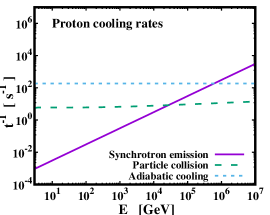
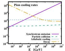
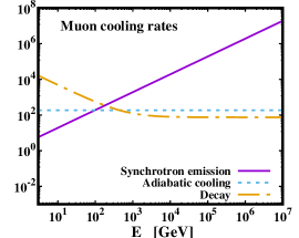
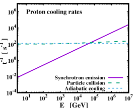
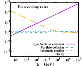
Figure 1: Cooling rates for the relativistic protons and the secondary particles ($\pi^{\pm}$, $\mu^{\pm}$) produced after the p-p mechanism takes place in LMC X-1 (1st row) and Cyg X-1 (2nd row).

As can be seen, the particle synchrotron losses become dominant for large energies with the particle mass setting the separation point. In the case of protons, due to their large mass, synchrotron losses are not dominant up to very high energies. This leads to a distribution with stable inclination matching the hot proton power-law exponent. On the other hand, for pions and muons, we see that the decay dominates the lower energy band and that is why the two curves in the respective graphs (corresponding to distributions considering energy losses along with the decay process only) progress similarly, especially for energies up to the decay rate stabilization. The synchrotron losses take off causing the smoother transition in the solid line’s case (with energy losses) compared to the dashed one (only decay).

After calculating all the necessary distributions, the neutrino and $\gamma$-ray emissivities as well as the corresponding intensities may be provided. For the LMC X-1 system, our results have shown that, the increase of the half-opening angle $\xi$ leads to a decrease in the $\gamma$-ray production, which is an expected result since the p-p collision rate drops with the jet’s expansion [6].

5 Summary and Conclusions

Black Hole X-ray binary systems (BHXRBs), consisting of a high mass compact object (black hole) and absorbing mass out of a companion star that results in an accretion disc formation, have been identified through their relativistic magnetohydrodynamical astrophysical flow ejection perpendicular to the aforementioned disc. This flow is mostly accelerated and collimated by the presence of a rather strong magnetic field which is initially attached to the rotational disc. A portion of the hadronic jet’s particles (mostlye protons) are accelerated to relativistic velocities through shock waves travelling across the jet. Then, a reaction chain takes place stemming from the inelastic $p-p$ interactions which leads to production of neutrinos and high energy $\gamma$-rays, both detectable at the terrestrial extremely sensitive detectors.

In this work, we focus mainly on the mechanisms and phenomena that affect highly the inelastic $p-p$ scattering and the generated secondary particles which participate afterwards in reaction chains leading to the emission of neutrinos and $\gamma$-rays. For two concrete examples, the Galactic Cygnus X-1 and the extragalactic LMC X-1 binary systems, we studied in more detail their cooling rates and energy distributions. Numerical simulations of neutrino emissivities and neutrino intensities will be publised elsewhere.

6 Acknowledgments

TSK acknowledges that this research is co-financed by Greece and the European Union (European Social Fund-ESF) through the Operational Programme ”Human Resources Development, Education and Lifelong Learning 2014- 2020” in the context of the project (MIS5047635).

References

References

- [1] Reynoso M M, Romero G E and Christiansen H R 2008 MNRAS 387 1745
- [2] Reynoso M M and Romero G E 2009 A&A 493 01
- [3] Smponias T and Kosmas O 2015 Adv. High Energy Phys. 2015 921757.
- [4] Smponias T and Kosmas O 2017 Adv. High Energy Phys. 2017 496274, arXiv:1706.03087 [astro-ph.HE].
- [5] Kosmas O T and Smponias T 2018 Adv. High Energy Phys. 2018 960296, arXiv:1808.00303 [astro-ph.HE].
- [6] Papavasileiou Th V, Kosmas O T, and Sinatkas J Unpublished results Adv. High Ener. Phys.
- [7] Papavasileiou Th V 2020 ”Production of neutrinos and cosmic rays from relativistic astrophysical magnetohydrodynamical jets”, MSc Thesis, University of Ioannina (unpublished).
- [8] Smponias T and Kosmas T S 2011 MNRAS 412 1320
- [9] Smponias T and Kosmas T S 2014 MNRAS 438 1014
- [10] Kelner S R, Aharonian F A and Bugayov V V 2006 Phys. Rev. D 74 034018
- [11] Orosz J A, Steeghs D, McClintock J E, et al. 2009 ApJ 697 573
- [12] Orosz J A et al. 2011 ApJ 742 84