A Computational Approach to Identification of Treatment Effects for Policy Evaluation

Abstract

For counterfactual policy evaluation, it is important to ensure that treatment parameters are relevant to policies in question. This is especially challenging under unobserved heterogeneity, as is well featured in the definition of the local average treatment effect (LATE). Being intrinsically local, the LATE is known to lack external validity in counterfactual environments. This paper investigates the possibility of extrapolating local treatment effects to different counterfactual settings when instrumental variables are only binary. We propose a novel framework to systematically calculate sharp nonparametric bounds on various policy-relevant treatment parameters that are defined as weighted averages of the marginal treatment effect (MTE). Our framework is flexible enough to fully incorporate statistical independence (rather than mean independence) of instruments and a large menu of identifying assumptions beyond the shape restrictions on the MTE that have been considered in prior studies. We apply our method to understand the effects of medical insurance policies on the use of medical services.

JEL Numbers: C14, C32, C33, C36

Keywords: Heterogeneous treatment effects, local average treatment effects, marginal treatment effects, extrapolation, partial identification, linear programming.

1 Introduction

For counterfactual policy evaluation, it is important to ensure that treatment parameters are relevant to the policies in question. This is especially challenging in the presence of unobserved heterogeneity. This challenge is well featured in the definition of the local average treatment effect (LATE). The LATE has been one of the most popular treatment parameters used by empirical researchers since it was introduced by Imbens and Angrist (1994). It induces a straightforward linear estimation method that requires only a binary instrumental variable (IV), and yet, allows for unrestricted treatment heterogeneity. The unfortunate feature of the LATE is that, as the name suggests, the parameter is intrinsically local, recovering the average treatment effect (ATE) for a specific subgroup of population called compliers. This feature leads to two major challenges in making the LATE a reliable parameter for counterfactual policy evaluation. First, the subpopulation for which the effect is measured (e.g., via randomized experiments) may not be the population of policy interest. Second, the definition of the subpopulation depends on the IV chosen, rendering the parameter even more difficult to extrapolate to targeted environments.

Dealing with the lack of external validity of the LATE has been an important theme in the literature. One approach in theoretical work (Angrist and Fernandez-Val (2010); Bertanha and Imbens (2019)) and empirical research (Dehejia et al. (2019); Muralidharan et al. (2019)) has been to show the similarity between complier and non-complier groups based on observables. This approach, however, cannot attend to possible unobservable discrepancies between these groups. Heckman and Vytlacil (2005) unify well-known treatment parameters by expressing them as weighted averages of what they define as the marginal treatment effect (MTE). This MTE framework has a great potential for extrapolation because a class of treatment parameters that are policy-relevant can also be generated as weighted averages of the MTE. The only obstacle is that the MTE is identified via a method called local IV (Heckman and Vytlacil (1999)), which requires the continuous variation of the IV that is sometime large depending on the target parameter. This in turn reflects the intrinsic difficulty of extrapolation when available exogenous variation is only discrete. Acknowledging this nature of the challenge, previous studies in the literature have proposed imposing shape restrictions on the MTE, which is a function of the treatment-selection unobservable, while allowing for binary instruments in the framework of Heckman and Vytlacil (2005). Brinch et al. (2017) introduce shape restrictions (e.g., linearity) on the MTE functions in an attempt to identify the LATE extrapolated to different subpopulations or to test for its external validity. In interesting recent work, Mogstad et al. (2018) propose a general partial identification framework where bounds on various policy-relevant treatment parameters can be obtained from a set of “IV-like estimands” that are directly identified from the data and routinely obtained in empirical work. Kowalski (2021) applies an approach similar to these studies to extrapolate the results from one health insurance experiment to an external setting.

This paper continues this pursuit and investigates the possibility of extrapolating local treatment parameters to different policy settings in the MTE framework when IVs are possibly only binary. We propose a computational approach to calculate sharp nonparametric bounds on various extrapolated treatment parameters for discrete and continuous outcomes. We use IVs that satisfy the statistical independence assumption conditional on covariates. The parameters are defined as weighted averages of the MTE. Examples include the ATE, the treatment effect on the treated, the LATE for subgroups induced by new policies, and the policy-relevant treatment effect (PRTE). We also show how to place in this procedure restrictions from a large menu of identifying assumptions beyond the shape restrictions considered in earlier work.

In this paper, we make four main contributions. First, we propose a novel framework for systematically calculating bounds on policy-relevant treatment parameters. We introduce the distribution of the latent state of the outcome-generating process conditional on the treatment-selection unobservable. This latent conditional distribution is the key ingredient for our analysis, as both the target parameter and the distribution of the observables can be written as linear functionals of it. Because the latent distribution is a fundamental quantity in the data-generating process, it is convenient to impose identifying assumptions. Having the latent distribution as a decision variable, we can formulate infinite-dimensional linear programming (LP) that produces bounds on a targeted treatment parameter. Our approach is reminiscent of Balke and Pearl (1997) and can be viewed as its generalization to the MTE framework. Balke and Pearl (1997) characterize bounds on the ATE using a binary outcome, treatment and instrument by introducing a LP approach with the latent response vector as the decision variable. The main distinction of our approach is that the latent distribution is conditioned on the selection unobservable, which makes the program infinite-dimensional, but is important for our extrapolation purpose. We also allow for both discrete and continuous $Y$. To make it feasible to solve the resulting infinite-dimensional program, we use a sieve-like approximation of the program and produce a finite-dimensional LP. We also develop a method to rescale the LP to resolve computational issues that arise with a large sieve dimension.

The use of approximation to construct an LP is similar to Mogstad et al. (2018)’s approach. However, the approach we take differs from theirs in the following way. While they use the MTE function (more precisely, each term in the MTE) as the main ingredient to relate IV-like estimands to target parameters, we use the latent distribution as our main building block to relate the full distribution of the data to target parameters. The main consequence of this difference is that we can exhaust the identifying power of statistical independence of IVs, while their approach can exploit mean independence. The two approaches are complementary. For example, when IVs are generated from randomized experiments, one can comfortably assume full independence, in which case our approach can be applied to enjoy the tighter bounds than those under mean independence. This can be useful when the external validity of experimental results is in question, making the extrapolation of the LATE desirable.

Second, we introduce identifying assumptions that have not been used in the context of the MTE framework or the LATE extrapolation. They include assumptions that there exist exogenous variables other than IVs. One of the main messages we hope to deliver in this paper is that, given the challenge of extrapolation, additional exogenous variation can be useful to conduct informative policy evaluation. We propose two types of exogenous variables that have been used in the literature in the context of identifying the ATE: Shaikh and Vytlacil (2011), Mourifié (2015), Han and Vytlacil (2017), Vuong and Xu (2017), and Han and Lee (2019) use the first type (entering the outcome and selection equations), and Vytlacil and Yildiz (2007), Liu et al. (2020), and Balat and Han (2020) use the second type (only entering the outcome equation). For example, the existence of the second type can be plausible when the agent has imperfect foresight when making the treatment selection decision. We utilize these variables in the context of the MTE framework. Moreover, while the existing papers on the ATE make use of these variables in combination with rank similarity, rank invariance, or additive separability, we show that they independently have identifying power for treatment parameters, including the ATE. In general, it may not be always easy to find such exogenous variables. But when the researcher does find it, it can be a more reliable source of identification than assumptions on counterfactual quantities, as the identifying power comes from the data rather than the researcher’s prior.

We also propose identifying assumptions that restrict treatment effect heterogeneity. In particular, we propose a range of uniformity assumptions that relate to rank similarity or rank invariance (Chernozhukov and Hansen (2005)) and monotone treatment response in Manski and Pepper (2000), including a novel identifying assumption, called rank dominance. The direction of endogeneity can also be incorporated in this MTE framework. This assumption is sometimes imposed in empirical work to characterize selection bias and has been shown to have identifying power for the ATE (Manski and Pepper (2000)).

Third, we show that our approach yields straightforward proof of the sharpness of the resulting bounds, no matter whether the outcome is discrete or continuous and whether additional identifying assumptions are imposed or not. This feature stems from the use of the latent conditional distribution in the linear programming and the convexity of the feasible set in the program. When the MTE itself is the target parameter, we distinguish between the notions of pointwise and uniform sharpness and argue why uniform sharpness is often difficult to achieve.

Fourth, as an application, we study the effects of insurance on medical service utilization by considering various counterfactual policies related to insurance coverage. The LATE for compliers and the bounds on the LATE for always-takers and never-takers reveal that possessing private insurance tend to have the largest effect on medical visits for never-takers, i.e., those who face higher insurance cost. This provides a policy implication that lowering the cost of private insurance is important, because the high cost might hinder people with most need from receiving adequate medical services.

The linear programming approach to partial identification of treatment effects was pioneered by Balke and Pearl (1997) and recently gained attention in the literature; see, e.g., Chiburis (2010a), Mogstad et al. (2018), Machado et al. (2019), Kamat (2019), Gunsilius (2019), Han (2019), Russell (2021), Han and Xu (2023). As these papers suggest, there are many settings, including ours, where analytical derivation of bounds is cumbersome or nearly impossible due to the complexity of the problems. Also, the computational approach can streamline the sensitivity analysis of a researcher without needing to analytically derive bounds and prove their sharpness whenever changing the set of identifying assumptions.

As concurrent work to ours, Marx (2020) also considers partial identification of policy-relevant treatment parameters in the MTE framework. In his paper, sharp analytical bounds are derived for treatment parameters for the subset of compliers, and the identifying power of rank similarity and covariates is explored for general treatment parameters. The current paper is similar to his in that we also fully exhaust statistical independence (rather than mean independence) and produce sharp bounds. However, our approach differs in a few important ways. First, we provide a computational framework that enables the systematic calculation of bounds. Second, with the computational approach, we produce bounds for a range of treatment parameters under various identifying assumptions that have not been previously explored in this context. Also, the computational approach makes it convenient to conduct sensitivity analyses with different sets of assumptions.

This paper proceeds as follows. The next section introduces the main observables, maintained assumptions, and parameters of interest. Section 3 defines the latent conditional probability and formulates the infinite-dimensional LP, and Section 4 introduces sieve approximation to the program. Section 5 establishes the connection between this paper and Mogstad et al. (2018). Section 6 introduces additional identifying assumptions and shows how they can easily be incorporated in the LP. So far, the analysis is given with discrete $Y$, which is extended to the case with continuous $Y$ in Section 7. Section 8 provides numerical illustrations, and Section 9 contains an empirical application. In the Appendix, Section A lists other examples of target parameters. Section B discusses (i) rescaling of the LP, (ii) the pointwise and uniform sharpness for the MTE bounds, (iii) the extension with continuous covariates, and (iv) estimation and inference. All proofs are contained in Section C. Additional numerical results can be found in Section D.

2 Assumptions and Target Parameters

Assume that we observe a discrete or continuous outcome $Y\in\mathcal{Y}\subseteq\mathbb{R}$, binary treatment $D\in\{0,1\}$, and possibly discrete instrument $Z\in\mathcal{Z}\subseteq\mathbb{R}$. The leading case is binary $Z$, which is common especially in randomized experiments. We may additionally observe an exogenous variable $W\in\mathcal{W}\subseteq\mathbb{R}$ and possibly endogenous covariates $X\in\mathcal{X}\subseteq\mathbb{R}^{d_{X}}$.

Let $Y(d)$ be the counterfactual outcome given $d$ and $Y(d,w)$ be the extended counterfactual outcome given $(d,w)$, which are consistent with the observed outcome: $Y=\sum_{d\in\{0,1\}}1\{D=d\}Y(d)=\sum_{d\in\{0,1\},w\in\mathcal{W}}1\{D=d,W=w\}Y(d,w)$.

Assumption EX.

For given $(d,w)\in\{0,1\}\times\mathcal{W}$, $(Y(d,w),U)\perp(Z,W)|X$.

When there is no $W$ this assumption and all below are understood as $W$ being degenerate. Assumption EX imposes the exclusion restriction and conditional statistical independence for $Z$ (and $W$). One of the contributions of this paper is to propose a framework that can make use of full independence instead of mean independence (Mogstad et al. (2018)) and show the identifying power of the former relative to the latter. This feature arises regardless of the existence of $W$. We formally discuss the identifying power of full independence relative to mean independence in Section 5. Also, note that Assumption EX imposes marginal independence rather than joint independence of $\{Y(d,w),U\}_{(d,w)\in\{0,1\}\times\mathcal{W}}\perp(Z,W)|X$.

We consider two different scenarios related to $W$: (a) $W$ directly affects $Y$ but not $D$ and (b) $W$ directly affects both $Y$ and $D$. Accordingly, we maintain the following assumptions.

Assumption SEL.

(a) $D=1\{U\leq P(Z,X)\}$ where $P(Z,X)\equiv\Pr[D=1|Z,X]$;
(b) $D=1\{U\leq P(Z,X,W)\}$ where $P(Z,X,W)\equiv\Pr[D=1|Z,X,W]$.

We introduce $W$ as an additional exogenous variable researchers may be equipped with in addition to the instrument $Z$. Given the challenge of extrapolation with minimal variation in $Z$, it would be important to search for additional exogenous variables. In the case of (a), such variables can be motivated by exogenous shocks that agents cannot fully anticipate at the time of making treatment choices. For example, let $Y$ be the earning and $D$ be the college attendance. In this example, $W$ can be a randomized job training program that directly affects $Y$ but whose lottery outcome cannot be foreseen when making the college decision. As another example, when $Y$ is the health outcome and $D$ is getting an insurance, $W$ can be random health or policy shocks that cannot be fully anticipated when making the insurance decision. In the context of generalized Roy models, (a) is consistent with agents’ limited information when comparing the potential outcomes of the two treatment states. We show the identifying power of $W$ even with its minimal variation. This is the first paper that formally uses this type of variable for identification in the MTE framework. Note that the requirement of reverse exclusion of $W$ in (a) can be tested from the data by inspecting whether $\Pr[D=1|Z,X,W]=\Pr[D=1|Z,X]$.

Assumption SEL imposes a selection model for $D$, which is important in motivating and interpreting marginal treatment effects later. This assumption is also equivalent to Imbens and Angrist (1994)’s monotonicity assumption (Vytlacil (2002)). We introduce the standard normalization that $U\sim Unif[0,1]$ conditional on $X=x$.

In Assumption SEL, Case (a) is where $W$ is a reversely excluded exogenous variable, which we call reverse IV. This type of exogenous variables was considered by Vytlacil and Yildiz (2007), Balat and Han (2020), and Liu et al. (2020). In Case (b), we show that a reverse IV is not necessary, and $W$ can be present in the selection equation. This type of exogenous variables was considered by Shaikh and Vytlacil (2011), Mourifié (2015), Han and Vytlacil (2017), Vuong and Xu (2017), and Han and Lee (2019). In both scenarios, however, we show that we can use $W$ for identification without necessarily invoking rank similarity, rank invariance, or additive separability in contrast to the above studies. We show this is possible due to the computational approach we take. Below, we combine the existence of $W$ with assumptions that are related to rank similarity. Another distinct feature of our approach in comparison to the prior studies is that we consider a broad class of the generalized LATEs as our target parameter, including the ATE considered in those studies. For notational simplicity, we focus on Case (a) henceforth; it is straightforward to draw analogous results for Case (b).

We aim to establish sharp bounds on various treatment parameters. Following Heckman and Vytlacil (2005), we express treatment parameters as integral equations of the MTE. The MTE is defined in our setting as

$$E[Y(1)-Y(0)|U=u,X=x],$$

where $Y(d)=Y(d,W)$. Similar to Mogstad et al. (2018), it is convenient to introduce the marginal treatment response (MTR) function

$$m_{d}(u,w,x) \equiv E[Y(d,w)|U=u,X=x]$$

where $W$ does not appear as a conditioning variable due to Assumption EX. Now, we define the target parameter $\tau$ to be the difference of the weighted averages of the MTRs:

$$\tau =E[\tau_{1}(Z,W,X)-\tau_{0}(Z,W,X)],$$ (2.1)

where

$$\tau_{d}(z,w,x) =\int m_{d}(u,w,x)\omega_{d}(u,z,x)du$$ (2.2)

by using $F_{U|X}(u|x)=u$, and $\omega_{d}(u,z,x)$ is a known weight specific to the parameter of interest. This definition agrees with the insight of Heckman and Vytlacil (2005). The target parameter includes a wide range of policy-relevant treatment parameters. We list a few examples of the target parameter here; other examples can be found in Table 5 in the Appendix.

Example 1.

With a Dirac delta function for a given value $u$ as the weight, the MTE itself can be a target parameter.

$$\tau_{MTE} =E[m_{1}(u,W,X)-m_{0}(u,W,X)]$$

Example 2.

The ATE can be a target parameter with $\omega_{d}(u,z,x)=1$ for any $(u,z,x)$.

$$\tau_{ATE}=E\left[\int_{0}^{1}m_{1}(u,W,X)du-\int_{0}^{1}m_{0}(u,W,X)du\right]$$

Example 3.

The generalized LATE is also a target parameter. Suppose we are interested in the LATE for individuals lying in $[\underline{u},\overline{u}]$. We assign the weight $\omega_{d}(u,z,x)=\frac{1(u\in[\underline{u},\overline{u}])}{\overline{u}-\underline{u}}$ for any $(u,z,x)$ , where the numerator excludes people outside this range and the denominator gives a weight to people within $[\underline{u},\overline{u}]$ according to their fraction in the whole population. The generalized LATE is expressed as:

$$\tau_{GLATE}=E\left[\int_{0}^{1}m_{1}(u,W,X)\frac{1(u\in[\underline{u},\overline{u}])}{\overline{u}-\underline{u}}du-\int_{0}^{1}m_{0}(u,W,X)\frac{1(u\in[\underline{u},\overline{u}])}{\overline{u}-\underline{u}}du\right]$$

Example 4.

The policy relevant treatment effect (PRTE) is a target parameter that is particularly useful for policy evaluation. It is defined as the welfare difference between two different policies. Let $Z$ and $Z^{\prime}$ be two instrument variables under two policies and $P(Z,X)$ and $P^{\prime}(Z^{\prime},X)$ be propensity scores under the two policies.

$$\tau_{PRTE} =E\Bigg{[}\int_{0}^{1}m_{1}(u,W,X)\frac{\Pr\left[u\leq P^{\prime}(Z^{\prime},X)\right]-\Pr\left[u\leq P(Z,X)\right]}{E\left[P^{\prime}(Z^{\prime},X)\right]-E\left[P(Z,X)\right]}du$$

$$-\int_{0}^{1}m_{0}(u,W,X)\frac{\text{$\Pr$}\left[u\leq P^{\prime}(Z^{\prime},X)\right]-\Pr\left[u\leq P(Z,X)\right]}{E\left[P^{\prime}(Z^{\prime},X)\right]-E\left[P(Z,X)\right]}du\Bigg{]}$$

To define a broader class of parameters beyond these examples, the weights $\omega_{0}$ and $\omega_{1}$ can be set asymmetrically. All the parameters we consider in this paper can be defined conditional on $X$ and $W$, although we omit them for succinctness.

Typically, a binary instrument is not sufficient in producing informative bounds on the target parameters. This is because a binary instrument has no extrapolative power for general non-compliers, e.g., always-takers and never-takers, but only identifies the effect for compliers. Prior studies have tried to overcome this challenge by imposing shape restrictions on the MTE (Cornelissen et al. (2016), Brinch et al. (2017), Mogstad et al. (2018), Kowalski (2021)), although these restrictions are not always empirically justified. Evidently, it would be useful to provide empirical researchers with a larger variety of assumptions so that it is easier to find justifiable assumptions that suit their specific examples.

The existence of additional exogenous variables embodied in Assumptions SEL and EX may be appealing as it can be warranted by data with less arbitrariness. We accompany Assumptions SEL and EX with an assumption that $W$ and $Z$ are relevant variables, which make the role of these variables more explicit.

Assumption R.

For given $x\in\mathcal{X}$, (i) $\Pr[Y(d,w)\neq Y(d,w^{\prime})|X=x]>0$ for some $d$ and $w\neq w^{\prime}$; (ii) either (a) $P(z,x)\neq P(z^{\prime},x)$ for $z\neq z^{\prime}$ and $0<P(z,x)<1$ for all $z$ or (b) $P(z,x,w)\neq P(z^{\prime},x,w)$ for $z\neq z^{\prime}$ and $0<P(z,x,w)<1$ for all $(z,w)$.

Assumption R(i) is a relevance condition for $W$ in determining $Y$. R(ii) is the standard relevance assumption for the instrument and the positivity assumption. We later show that under Assumptions SEL, EX and R, the variation of $W$ (in addition to $Z$) is a useful source for extrapolation and narrowing the bounds on target parameters.

3 Distribution of Latent State and Infinite-Dimensional Linear Program

Our goal is to provide a systematic framework to calculate bounds on the target parameters, which is easy to incorporate various identifying assumptions. To this end and as a crucial first step of our analysis, we define a state variable that determines a specific mapping of

$$(d,w) \mapsto y$$ (3.1)

for discrete $y\in\mathcal{Y}=\{y_{1},...,y_{L}\}$. We discuss the extension with continuously distributed $Y$ in Section 7. Given that $d$ is binary and assuming $w$ is also binary, there are $L^{4}$ possible states or maps from $(d,w)$ onto $y$. Using the extended counterfactual outcome $Y(d,w)$, define a latent vector $\epsilon$ as

$$\epsilon \equiv(Y(0,0),Y(0,1),Y(1,0),Y(1,1))$$

and its realized value as $e\equiv(y(0,0),y(0,1),y(1,0),y(1,1))\in\mathcal{E}=\mathcal{Y}^{4}$. Then, each value of $e$ represents each possible state. Table 1 lists all 16 maps in a leading case of binary $y$ with $\mathcal{Y}=\{0,1\}$.

#	$d$	$w$	$Y(d,w)$
1	0	0	0
	0	1	0
	1	0	0
	1	1	0
2	0	0	1
	0	1	0
	1	0	0
	1	1	0
3	0	0	0
	0	1	1
	1	0	0
	1	1	0
4	0	0	1
	0	1	1
	1	0	0
	1	1	0

#	$d$	$w$	$Y(d,w)$
5	0	0	0
	0	1	0
	1	0	1
	1	1	0
6	0	0	1
	0	1	0
	1	0	1
	1	1	0
7	0	0	0
	0	1	1
	1	0	1
	1	1	0
8	0	0	1
	0	1	1
	1	0	1
	1	1	0

#	$d$	$w$	$Y(d,w)$
9	0	0	0
	0	1	0
	1	0	0
	1	1	1
10	0	0	1
	0	1	0
	1	0	0
	1	1	1
11	0	0	0
	0	1	1
	1	0	0
	1	1	1
12	0	0	1
	0	1	1
	1	0	0
	1	1	1

#	$d$	$w$	$Y(d,w)$
13	0	0	0
	0	1	0
	1	0	1
	1	1	1
14	0	0	1
	0	1	0
	1	0	1
	1	1	1
15	0	0	0
	0	1	1
	1	0	1
	1	1	1
16	0	0	1
	0	1	1
	1	0	1
	1	1	1

Table 1: All Possible Maps from $(d,w)$ to $y\in\{0,1\}$

Now, as a key component of our LP, we define the probability mass function of $\epsilon$ conditional on $(U,X)$: for $e\in\mathcal{E}$,

$$q(e|u,x) \equiv\Pr[\epsilon=e|U=u,X=x]$$ (3.2)

with $\sum_{e\in\mathcal{E}}q(e|u,x)=1$ for any $(u,x)$. The quantity $q(e|u,x)$ captures the joint distribution of $(\epsilon,U)$ and thus reflects endogenous treatment selection. It is shown below that this latent conditional probability is a building block for various treatment parameters and thus serves as the decision variable in the LP. The introduction of $q(e|u,x)$ distinguishes our approach from those in Balke and Pearl (1997) and Mogstad et al. (2018). Since the probability is conditional on continuously distributed $U$, the simple finite-dimensional linear programming approach of Balke and Pearl (1997) is no longer applicable. Instead, we use an approximation method similar to Mogstad et al. (2018). However, Mogstad et al. (2018) uses the MTR function as a building block for treatment parameters and introduces the “IV-like” estimands as a means of funneling the information from the data. Unlike in Mogstad et al. (2018), $q(e|u,x)$ can be directly related to the distribution of data. This allows us to (i) fully exhaust the full independence assumption, (ii) facilitate proving sharpness and (iii) incorporating a large menu of additional identifying assumptions.

In the remaining section and the next section, we focus on binary $Y$ for simplicity; the extension to general discrete $Y$ is straightforward and is discussed in Section 5; continuous $Y$ is considered in Section 7. Also, we will mostly focus on binary $W$ and discrete $X$ for expositional simplicity. Section B.3 in the Appendix extends the framework to incorporate continuously distributed $X$; it is also straightforward to extend to allow for general discrete variable $W$. By (3.2), note that

$$\Pr[Y(d,w)=1|U=u,X=x] =\Pr[\epsilon\in\{e\in\mathcal{E}:y(d,w)=1\}|U=u,X=x]$$

$$=\sum_{e\in\mathcal{E}:y(d,w)=1}q(e|u,x).$$

Therefore, the MTR can be expressed as

$$m_{d}(u,w,x) =\sum_{e:y(d,w)=1}q(e|u,x).$$ (3.3)

Combining (2.2) and (3.3), we have $\tau_{d}(z,w,x)=\sum_{e:y(d,w)=1}\int q(e|u,x)\omega_{d}(u,z,x)du$, and thus the target parameter $\tau=E[\tau_{1}(Z,W,X)]-E[\tau_{0}(Z,W,X)]$ in (2.1) can be written as

$$\tau =E\left[\sum_{e:y(1,W)=1}\int q(e|u,X)\omega_{1}(u,Z,X)du-\sum_{e:y(0,W)=1}\int q(e|u,X)\omega_{0}(u,Z,X)du\right]$$ (3.4)

for some $q$ that satisfies the properties of probability.

The goal of this paper is to (at least partially) infer the target parameter $\tau$ based on the data, i.e., the distribution of $(Y,D,Z,W,X)$. The key insight is that there are observationally equivalent $q(e|u,x)$’s that are consistent with the data, which in turn produces observationally equivalent $\tau$’s that define the identified set.

Let $p(y,d|z,w,x)\equiv\Pr[Y=y,D=d|Z=z,W=w,X=x]$ be the observed conditional probability. This data distribution imposes restrictions on $q(e|u,x)$. For instance, for $D=1$,

$$p(y,1|z,w,x) =\Pr[Y(1,w)=y,U\leq P(z,x)|Z=z,W=w,X=x]$$

$$=\Pr[Y(1,w)=y,U\leq P(z,x)|X=x]$$

by Assumption EX, but

$$\Pr[Y(1,w)=y,U\leq P(z,x)|X=x] =\int_{0}^{P(z,x)}\Pr[Y(1,w)=y|U=u,X=x]du$$

$$=\sum_{e:y(1,w)=y}\int_{0}^{P(z,x)}q(e|u,x)du,$$ (3.5)

where the second equality is by $\Pr[Y(d,w)=y|U=u,X=x]=\sum_{e:y(d,w)=y}q(e|u,x)$.

To define the identified set for $\tau$, we introduce some simplifying notation. Let $q(u)\equiv\{q(e|u,x)\}_{e\in\mathcal{\mathcal{E}},x\in\mathcal{X}}$ and

$$\mathcal{Q}\equiv\{q(\cdot):\sum_{e\in\mathcal{E}}q(e|u,x)=1\text{ and }q(e|u,x)\geq 0\text{ }\forall(e,u,x)\}$$

be the class of $q(u)$, and let

$$p\equiv\{p(1,d|z,w,x)\}_{(d,z,w,x)\in\{0,1\}\times\mathcal{Z}\times\mathcal{W}\times\mathcal{X}}.$$

Also, let $R_{\omega}:\mathcal{Q}\rightarrow\mathbb{R}$ and $R_{0}:\mathcal{Q}\rightarrow\mathbb{R}^{d_{p}}$ (with $d_{p}$ being the dimension of $p$) denote the linear operators of $q(\cdot)$ that satisfy

$$R_{\omega}q \equiv E\left[\sum_{e:y(1,W)=1}\int q(e|u,X)\omega_{1}(u,Z,X)du-\sum_{e:y(0,W)=1}\int q(e|u,X)\omega_{0}(u,Z,X)du\right],$$

$$R_{0}q \equiv\left\{\sum_{e:y(d,w)=1}\int_{\mathcal{U}_{z,x}^{d}}q(e|u,x)du\right\}_{(d,z,w,x)\in\{0,1\}\times\mathcal{Z}\times\mathcal{W}\times\mathcal{X}},$$

where $\mathcal{U}_{z,x}^{d}$ denotes the intervals $\mathcal{U}_{z,x}^{1}\equiv[0,P(z,x)]$ and $\mathcal{U}_{z,x}^{0}\equiv(P(z,x),1]$. Then, we can characterize the baseline identified set for $\tau$ where we only impose modeling primitives. Later, we show how to characterize the identified set with additional assumptions introduced in Section 6.

Definition 3.1.

Suppose Assumptions EX and SEL(a) hold. The identified set of $\tau$ is defined as

$$\mathcal{T}^{*} \equiv\{\tau\in\mathbb{R}:\tau=R_{\omega}q\text{ for some }q\in\mathcal{Q}\text{ such that }R_{0}q=p\}.$$

In what follows, we formulate the infinite-dimensional LP ($\infty$-LP) that characterizes $\mathcal{T}^{*}$. This program conceptualizes sharp bounds on $\tau$ from the data and the maintained assumptions (Assumptions SEL and EX). The upper and lower bounds on $\tau$ are defined as

$$\overline{\tau}= \sup_{q\in\mathcal{Q}}R_{\omega}q, \infty$$ (-LP1)

$$\underline{\tau}= \inf_{q\in\mathcal{Q}}R_{\omega}q, \infty$$ (-LP2)

subject to

$$R_{0}q =p. \infty$$ (-LP3)

Observe that the set of constraints ($\infty$-LP3) does not include

$$\sum_{e:y(d,w)=0}\int_{\mathcal{U}_{z,x}^{d}}q(e|u,x)du =p(0,d|z,w,x)\qquad\forall(d,z,w,x).$$ (3.6)

This is because we know a priori that they are redundant in the sense that they do not further restrict the feasible set, namely, the set of $q(e|u,x)$’s that satisfy all the constraints ($q\in\mathcal{Q}$ and ($\infty$-LP3)).

Lemma 3.1.

In the linear program ($\infty$-LP1)–($\infty$-LP3), the feasible set defined by $q\in\mathcal{Q}$ and ($\infty$-LP3) is identical to the feasible set defined by $q\in\mathcal{Q}$, ($\infty$-LP3), and (3.6).

Theorem 3.1.

Under Assumptions SEL and EX, suppose $\mathcal{T}^{*}$ is non-empty. Then, the bounds $[\underline{\tau},\overline{\tau}]$ in ($\infty$-LP1)–($\infty$-LP3) are sharp for the target parameter $\tau$, that is, $cl(\mathcal{T}^{*})=[\underline{\tau},\overline{\tau}]$, where $cl(\cdot)$ is the closure of a set.

The result of this theorem is immediate due to the convexity of the feasible set $\{q:q\in\mathcal{Q}\}\cap\{q:R_{0}q=p\}$ in the LP and the linearity of $R_{\omega}q$ in $q$, which implies that $[\underline{\tau},\overline{\tau}]$ is convex.

4 Sieve Approximation and Finite-Dimensional Linear Programming

Although conceptually useful, the LP ($\infty$-LP1)–($\infty$-LP3) is not feasible in practice because $\mathcal{Q}$ is an infinite-dimensional space. In this section, we approximate ($\infty$-LP1)–($\infty$-LP3) with a finite-dimensional LP via a sieve approximation of the conditional probability $q(e|u,x)$. We use Bernstein polynomials as the sieve basis. Bernstein polynomials are useful in imposing restrictions on the original function (Joy (2000); Chen et al. (2011); Chen et al. (2017)) and therefore have been introduced in the context of linear programming (Mogstad et al. (2018); Mogstad et al. (2021); Masten and Poirier (2021)). Bernstein approximation based on those polynomials possesses the property of being “shape-preserving,” which effectively prevent undesired distortions from the original function’s shape properties (Goodman (1989); Carnicer and Pena (1993); Goodman et al. (1999)).

Consider the following sieve approximation of $q(e|u,x)$ using Bernstein polynomials of order $K$

$$q(e|u,x) \approx\sum_{k=1}^{K}\theta_{k}^{e,x}b_{k}(u),$$

where $b_{k}(u)\equiv b_{k,K}(u)\equiv\tbinom{K}{k}u^{k}(1-u)^{K-k}$ is a univariate Bernstein basis, $\theta_{k}^{e,x}\equiv\theta_{k,K}^{e,x}\equiv q(e|k/K,x)$ is its coefficient, and $K$ is finite. By using this approximation, we implicitly impose smoothness in $q(e|\cdot,x)$. Note that discrete $x$ can index $\theta$, because $q(e|u,x)$ is a saturated function of $x$. By the definition of the Bernstein coefficient, for any $(e,x)$, it satisfies $q(e|u,x)\geq 0$ for all $u$ if and only if $\theta_{k}^{e,x}\geq 0$ for all $k$. Also, $\sum_{e\in\mathcal{E}}q(e|u,x)=1$ for all $(u,x)$ is approximately equivalent to $\sum_{e\in\mathcal{E}}\theta_{k}^{e,x}=1$ for all $(k,x)$. To see this, first, $\sum_{e\in\mathcal{E}}q(e|u,x)=1$ for all $(u,x)$ implies $\sum_{e\in\mathcal{E}}\theta_{k}^{e,x}=\sum_{e\in\mathcal{E}}q(e|k/K,x)=1$ for all $(k,x)$. Conversely, when $\sum_{e\in\mathcal{E}}\theta_{k}^{e,x}=1$ for all $(k,x)$,

$$\sum_{e\in\mathcal{E}}q(e|u,x) \approx\sum_{e\in\mathcal{E}}\sum_{k=1}^{K}\theta_{k}^{e,x}b_{k}(u)=\sum_{k=1}^{K}b_{k}(u)=1$$

by the binomial theorem (Coolidge (1949)). Motivated by this approximation, we formally define the following sieve space for $\mathcal{Q}$:

$$\mathcal{Q}_{K} \equiv\left\{\Big{\{}\sum_{k=1}^{K}\theta_{k}^{e,x}b_{k}(u)\Big{\}}_{e\in\mathcal{E}}:\sum_{e\in\mathcal{E}}\theta_{k}^{e,x}=1\text{ and }\theta_{k}^{e,x}\geq 0\text{ }\forall(e,k,x)\right\}\subseteq\mathcal{Q}.$$ (4.1)

Let $\mathcal{K}\equiv\{1,...,K\}$ and $p(z,w,x)\equiv\Pr[Z=z,W=w,X=x]$. For $q\in\mathcal{Q}_{K}$, by (3.4) and (4.1), the target parameter $\tau=E[\tau_{1}(Z,W,X)]-E[\tau_{0}(Z,W,X)]$ can be expressed with

$$E[\tau_{d}(Z,W,X)] =\sum_{(w,x)\in\mathcal{W\times\mathcal{X}}}\sum_{e:y(d,w)=1}\sum_{k\in\mathcal{K}}\theta_{k}^{e,x}\gamma_{k}^{d}(w,x),$$ (4.2)

where $\gamma_{k}^{d}(w,x)\equiv\sum_{z\in\{0,1\}}p(z,w,x)\int b_{k}(u)\omega_{d}(u,z,x)du$. Also, for $q\in\mathcal{Q}_{K}$ and $D=1$, by (3.5), we have

$$p(y,1|z,w,x) =\sum_{e:y(1,w)=y}\sum_{k\in\mathcal{K}}\theta_{k}^{e,x}\delta_{k}^{1}(z,x),$$ (4.3)

where $\delta_{k}^{d}(z,x)\equiv\int_{\mathcal{U}_{z,x}^{d}}b_{k}(u)du$.

From (4.2) and (4.3), we can expect that a finite-dimensional LP can be obtained with respect to $\theta_{k}^{e,x}$. Let $\theta\equiv\{\theta_{k}^{e,x}\}_{(e,k,x)\in\mathcal{E}\times\mathcal{K}\times\mathcal{X}}$ and let

$$\Theta_{K} \equiv\left\{\theta:\sum_{e\in\mathcal{E}}\theta_{k}^{e,x}=1\text{ and }\theta_{k}^{e,x}\geq 0\text{ }\forall(e,k,x)\in\mathcal{E}\times\mathcal{K}\times\mathcal{X}\right\}.$$

Then, we can formulate the following finite-dimensional LP that corresponds to the $\infty$-LP in ($\infty$-LP1)–($\infty$-LP3):

$$\overline{\tau}_{K} =\max_{\theta\in\Theta_{K}}\sum_{(k,w,x)\in\mathcal{K\times\mathcal{W}\times\mathcal{X}}}\Big{\{}\sum_{e:y(1,w)=1}\theta_{k}^{e,x}\gamma_{k}^{1}(w,x)-\sum_{e:y(0,w)=1}\theta_{k}^{e,x}\gamma_{k}^{0}(w,x)\Big{\}}$$ (LP1)

$$\underline{\tau}_{K} =\min_{\theta\in\Theta_{K}}\sum_{(k,w,x)\in\mathcal{K\times\mathcal{W}\times\mathcal{X}}}\Big{\{}\sum_{e:y(1,w)=1}\theta_{k}^{e,x}\gamma_{k}^{1}(w,x)-\sum_{e:y(0,w)=1}\theta_{k}^{e,x}\gamma_{k}^{0}(w,x)\Big{\}}$$ (LP2)

subject to

$$\sum_{e:y(d,w)=1}\sum_{k\in\mathcal{K}}\theta_{k}^{e,x}\delta_{k}^{d}(z,x) =p(1,d|z,w,x)\qquad\forall(d,z,w,x)\in\{0,1\}\times\mathcal{Z}\times\mathcal{W}\times\mathcal{X}.$$ (LP3)

One of the advantages of LP is that it is computationally very easy to solve using standard algorithms, such as the simplex algorithm. Assuming binary $W$ and $X$ and setting $K=50$, we have $\dim(\theta)=1632$, and it takes less than 3 seconds to calculate $\overline{\tau}_{K}$ and $\underline{\tau}_{K}$ with moderate computing power. The increase in the support of $\mathcal{W}$ (and thus the number of maps (3.1)) only linearly increases the computation time.

The important remaining question is how to choose $K$ in practice. We discuss this issue in Section 8. Also, when $K$ is too large, coefficients on $\theta_{k}^{e,x}$ in (LP3) tend to take values with incomparable orders of magnitude, which may cause common optimization algorithms to arbitrarily drop small values. To address this, we propose a rescaling method in Section B.1. Finally, extending Proposition 4 in Mogstad et al. (2018), we may exactly calculate $\overline{\tau}$ and $\underline{\tau}$ (i.e., $\overline{\tau}=\overline{\tau}_{K}$ and $\underline{\tau}=\underline{\tau}_{K}$) under the assumptions that (i) the weight function $\omega_{d}(u,z,x)$ is piece-wise constant in $u$ and (ii) the constant spline that provides the best mean squared error approximation of $q(e|u,x)$ satisfies all the maintained assumptions (possibly including the identifying assumptions introduced later) that $q(e|u,x)$ itself satisfies; see Mogstad et al. (2018) for details.

5 The Use of Statistical Independence

The framework proposed in this paper allows us to systematically calculate sharp bounds of treatment parameters using the (conditional) statistical independence of $Z$ and $W$ (Assumption EX). This is possible because the full distribution from the data enters the LP. This is in contrast to the approach in Mogstad et al. (2018) who utilize the first moment information of the data and exploit mean independence of $Z$ in their bound analysis. The full independence assumption is common in the nonparametric treatment effect literature and can be justified by, for example, IVs generated by randomized experiments. This section formally show the identifying power of full independence and, more importantly, how our framework allows us to make use of it to produce sharp bounds. To this end, we compare our approach with Mogstad et al. (2018)’s and show when the identified sets coincide and when they do not. We first focus on a simple case where $Z$ is the only exogenous variable. Then, we discuss how $W$ can add further identifying power.

To help the reader, we restate the maintained assumption in Mogstad et al. (2018) in terms of our notation:

Assumptions I (Mogstad et al. (2019)).

I.1. $U\perp Z|X$; I.2. $E[Y(d)|Z,X,U]=E[Y(d)|X,U]$ and $E[Y(d)^{2}]<\infty$ for $d\in\{0,1\}$; I.3. $U$ is continuously distributed conditional on $X$.

Assumption I.2 imposes mean independence of the instrument $Z$. On the other hand Assumption EX (after suppressing $W$ for clear comparison) implies $Y(d)\perp Z|X,U$, namely, statistical independence of $Z$. Therefore, we can expect that the latter has stronger identifying power. Below, we show that the LP constructed with $q$ being the choice variable instead of the MTR function $m_{d}$ enables us to exploit this extra identifying power.

In Mogstad et al. (2018) the IV-like estimands are the channel through which the data enters to restrict the set of $m_{d}$. They show (their Proposition 3) that if the IV-like estimands are carefully chosen, then the resulting set of $m_{d}$ is equivalent to the set of $m_{d}$ that are consistent with

$$E[Y|D=0,Z,X]=E[Y_{0}|U>p(Z,X),Z,X]=\frac{1}{1-P(Z,X)}\int_{p(Z,X)}^{1}m_{0}(u,X)du,$$ (5.1)

$$E[Y|D=1,Z,X]=E[Y_{1}|U\leq p(Z,X),Z,X]=\frac{1}{P(Z,X)}\int_{0}^{p(Z,X)}m_{1}(u,X)du.$$ (5.2)

Therefore, assuming such IV-like estimands are chosen, we can define their identified set as

$$\mathcal{M}_{id}=\Big{\{}m=(m_{0},m_{1}),m_{0},m_{1}\in L^{2}:m_{0},m_{1}\text{ satisfies equation (\ref{eq: infoset0}) and (\ref{eq: infoset1}) a.s.}\Big{\}}.$$

Note that this set is the result of funneling the information from data via the conditional means.

When $Y$ is binary, the mean and full independence assumptions are equivalent. Therefore we expect to find no difference in the resulting identified sets of treatment parameters between the two methods. We show this by comparing the identified set of the MTR functions $\mathcal{M}_{id}$ used in Mogstad et al. (2018) and the set of MTR functions derived from the feasible set in the LP proposed in the current paper (denoted as $\mathcal{M}_{f}$ below). More importantly, as soon as $Y$ departs from binarity, we show that $\mathcal{M}_{f}$ is a proper subset $\mathcal{M}_{id}$.

For comparison, define the feasible set $\mathcal{Q}_{f}$ of our proposed LP as

$$\mathcal{Q}_{f}=\Big{\{}q\in L^{2}([0,1]):q\in\mathcal{Q}\text{ and satisfies equation }(\ref{eq:constr})\Big{\}},$$

where $w$ is suppressed from ($\infty$-LP3). To establish the connection with $\mathcal{M}_{id}$, we construct the set of MTR functions based on $\mathcal{Q}_{f}$. For this purpose, we drop $W$ from the setting and redefine $\epsilon\equiv(Y(0),Y(1))$ and $e\equiv(y(0),y(1))$:

$$\mathcal{M}_{f}=\Big{\{}m=(m_{0},m_{1}):m_{d}(u,x)=\sum_{y\in\mathcal{Y}}y\sum_{e:y(d)=y}q(e|u,x),d=\{0,1\},q\in\mathcal{Q}_{f}\Big{\}}.$$

Then the following holds:

Theorem 5.1.

Suppose $\mathcal{Y}=\{0,1\}$. Under Assumptions SEL and EX, $\mathcal{M}_{f}=\mathcal{M}_{id}$.

Theorem 5.1 demonstrates that, when $Y$ is binary, the constraint used in our LP approach captures the same information as the constraint defined by the IV-like estimands that are appropriately selected. Consistent with Proposition 3 in Mogstad et al. (2018), $\mathcal{M}_{f}$ and $\mathcal{M}_{id}$ are sharp in this case.

When $Y$ is non-binary and we continue to impose statistical independence, the above equivalence breaks down. That is, unlike $\mathcal{M}_{id}$, $\mathcal{Q}_{f}$ exploits the full data distribution and the statistical independence assumption. We formally show this with $\mathcal{Y}=\{y_{1},...,y_{L}\}$. We accordingly redefine $p$ and $R_{0}$ in ($\infty$-LP3) (i.e., $R_{0}q=p$) in the definition of $\mathcal{Q}_{f}$ as

$$p \equiv\{p(y,d|z,x)\}_{(y,d,z,x)\in\mathcal{Y}\times\{0,1\}\times\mathcal{Z}\times\mathcal{X}},$$

$$R_{0}q \equiv\left\{\sum_{e:y(d)=y}\int_{\mathcal{U}_{z,x}^{d}}q(e|u,x)du\right\}_{(y,d,z,x)\in\mathcal{Y}\times\{0,1\}\times\mathcal{Z}\times\mathcal{X}},$$

without excluding redundant constraints and suppressing $w$ for simplicity. We introduce a technical assumption.

Assumption EC.

(i) $P(z,x)$ is upper semicontinuous on compact $\mathcal{Z}\times\mathcal{X}$; (ii) $\mathcal{Q}_{f}\subset L^{2}([0,1])$ is equicontinuous.

Theorem 5.2.

Suppose $\mathcal{Y}=\{y_{1},...,y_{L}\}$ with arbitrary $L\geq 3$. Under Assumptions SEL, EX and CT, $\mathcal{M}_{f}\subsetneq\mathcal{M}_{id}$.

When $Y$ takes more than two values, $\mathcal{Q}_{f}$ continues to exploit the full independence assumption and as shown in Theorem 3.1, $\mathcal{M}_{f}$ is sharp. Note $\mathcal{M}_{id}$ is a strict outer set of $\mathcal{M}_{f}$ because the former only exploits the first moment implication of full independence. This intuition also suggests that the case of continuous $Y$ would deliver a similar result as in Theorem 5.2. Theorems 5.1 and 5.2 corroborate the simulation results in Section 8.2. The simulation results for continuous $Y$ can be found in Section D.1.

Finally, consider the case where $W$ is also present and satisfies Assumptions EX and SEL. After proper modification of their assumptions (i.e., $U\perp(Z,W)|X$ and $E[Y(d)|Z,W,X,U]=E[Y(d)|X,U]$), Mogstad et al. (2018)’s framework may be able to use the exogenous variation of $W$. This can be done by using the moments $E[Y|D=d,Z,W,X]$ ($d=0,1$) as inputs in (5.1) and (5.2). However, by the same argument as the one above for $Z$, the full independence assumption with respect to $W$ will have a stronger identifying power than mean independence. When $Y$ is beyond binary, our framework can exploit this. The two frameworks also differ in how other additional identifying assumptions can be incorporated in the procedures. This point appears as Remark 6.1 in the next section.

Remark 5.1 (Manski’s Bounds).

When the ATE is the target parameter, the findings of this section has implications on the comparison of Manski (1990)’s bounds and our bounds (with no additional assumptions). Manski (1990) assumes the mean independence of exogenous variables. It is shown by Heckman and Vytlacil (2001) that Manski’s bounds coincide with their bounds, which should also be equivalent to Mogstad et al. (2018)’s bounds (with no additional assumptions). Therefore, Theorem 5.2 implies that, under the full independence assumption, our procedure produces the ATE bounds that are narrower than Manski’s bounds.

6 Incorporating Additional Identifying Assumptions

6.1 Additional Identifying Assumptions

In addition to Assumptions SEL, EX and R, researchers may be willing to restrict the degree of treatment heterogeneity, the direction of endogeneity, or the shape of the MTR functions. Although not necessary, such restrictions play significant roles in yielding informative bounds, especially given the challenge of extrapolating the LATE with minimal variation of the exogenous variables. Among the proposed assumptions, researchers want to use those that they deem plausible in given applications. Also, we provide only a few examples of assumptions here; we believe our proposed framework may open a venue for other assumptions we have not explored.

6.1.1 Restrictions on Treatment Heterogeneity

We present a range of restrictions on treatment heterogeneity in the order of stringency starting from the strongest.

Assumption U^∗.

For every $w,w^{\prime}\in\mathcal{W}$ and $x\in\mathcal{X}$, either $\Pr[Y(1,w)\geq Y(0,w^{\prime})|X=x]=1$ or $\Pr[Y(1,w)\leq Y(0,w^{\prime})|X=x]=1$.

The following assumption is weaker than Assumption U^∗.

Assumption U.

For every $w\in\mathcal{W}$ and $x\in\mathcal{X}$, either $\Pr[Y(1,w)\geq Y(0,w)|X=x]=1$ or $\Pr[Y(1,w)\leq Y(0,w)|X=x]=1$.

When $W$ is not available at all, this assumption can be understood with $\mathcal{W}$ being degenerate. In Assumption U^∗, $w$ and $w^{\prime}$ may be the same or different, i.e., the uniformity is for all combinations of $(w,w^{\prime})\in\{(0,0),(1,1),(1,0),(0,1)\}$. Therefore, Assumption U^∗ implies Assumption U. Assumptions U and U^∗ posit that individuals present uniformity in the sense that the treatment either weakly increases the outcome for all individuals or decreases it for all individuals. Intuitively, Assumption U^∗ is stronger because the uniformity remains to hold even under an outcome shift via $w\neq w^{\prime}$; this may hold when the treatment effect is strong across individuals. Assumptions U and U^∗ share insights with the monotone treatment response assumption that is introduced to bound the ATE in Manski (1997) and Manski and Pepper (2000). Assumptions U and U^∗ are also related to rank invariance considered in the literature (e.g., Chernozhukov and Hansen (2005), Marx (2020)). To see this, consider binary $Y$ and a structural model $Y=1[s(D,W)\geq V_{D}]$ with $V_{D}\equiv DV_{1}+(1-D)V_{0}$ (suppressing $X$). When rank invariance ($V_{1}=V_{0}\equiv V$) holds, Assumption U^∗ holds (and thus Assumption U) because either $P[s(1,w)<V,s(0,w^{\prime})\geq V]=0$ or $P[s(1,w)\geq V,s(0,w^{\prime})<V]=0$. On the other hand, Assumption U^∗ can still hold even if $V_{1}\neq V_{0}$ when, for example, the distribution of $(V_{1},V_{0})$ is concentrated around $45^{\circ}$ line. Therefore the converse is not true. It is important to note that Assumptions U and U^∗ still allow treatment heterogeneity in terms of $X$ (and similarly of $W$). For instance, Assumption U allows that $Y(1,w)\geq Y(0,w)$ a.s. for $X=x$ but $Y(1,w)\leq Y(0,w)$ a.s. for $X=x^{\prime}$. Assumption U is also used, for example, in Chiburis (2010b) although his focus is bounds on the ATE with binary $Y$.

In fact, it is possible to further weaken Assumption U. To motivate this with binary $Y$, we state Assumption U as follows (suppressing $X$): for every $w$, either $P[Y(1,w)=0,Y(0,w)=1]=0$ or $P[Y(1,w)=1,Y(0,w)=0]=0$. In other words, all individuals respond weakly monotonically to the treatment in the sense that there is no (strictly) negative-treatment-response type or positive-treatment-response type. By iterated expectation, Assumption U holds if and only if either $P[Y(1,w)=0,Y(0,w)=1|U]=0$ a.s. or $P[Y(1,w)=1,Y(0,w)=0|U]=0$ a.s. Then this assumption can be relaxed by allowing for the existence of both types in the population and instead assuming the dominance of one of the types over the other: for example, $P[Y(1,w)=1,Y(0,w)=0|U]>P[Y(1,w)=0,Y(0,w)=1|U]$ a.s. For general $Y$, such an assumption is written as follows (ignoring a measure zero set of $U$):

Assumption U⁰.

For every $w\in\mathcal{W}$ and $x\in\mathcal{X}$, either $P[Y(1,w)\geq Y(0,w)|U=u,X=x]\geq P[Y(1,w)\leq Y(0,w)|U=u,X=x]$ for all $u$ or $P[Y(1,w)\geq Y(0,w)|U=u,X=x]\leq P[Y(1,w)\leq Y(0,w)|U=u,X=x]$ for all $u$.

Assumption U⁰ is weaker than Assumption U, because when $P[Y(1,w)\leq Y(0,w)|X=x]=0$, Assumption U⁰ trivially holds. Compared to Assumption U, Assumption U⁰ allows further treatment heterogeneity in that positive- and negative-treatment-response types can both present in the population, but we impose a uniform order on the probabilities of effect sign across individuals. Researchers may be more comfortable with this assumption than complete uniformity. This paper is the first to propose to use this restriction in the identification of treatment effects. We call assumptions of this type rank dominance.

We show that the directions in Assumptions U^∗–U⁰ may be learned from the data. Suppress $X$ for simplicity and let $Z\in\{0,1\}$. Let $\tau_{LATE}(w,w^{\prime})\equiv E[Y(1,w)-Y(0,w^{\prime})|P(0)\leq U\leq P(1)]$ be the LATE defined using the extended counterfactual outcome $Y(d,w)$ assuming Assumption SEL(a) and $P(1)>P(0)$; the definition of $\tau_{LATE}(w,w^{\prime})$ under Assumption SEL(b) is analogous.

Lemma 6.1.

Suppose Assumptions SEL and EX hold and $Z\in\{0,1\}$. Then, (i) $\tau_{LATE}(w,w^{\prime})$ is identified for any $w,w^{\prime}\in\mathcal{W}$. Based on this, (ii) the directions in Assumptions U^∗ and U are identified; (iii) additionally, when $Y\in\{0,1\}$, the direction in Assumption U⁰ is identified.

The practical implication of this lemma is that the direction of each assumption will be detected by the feasibility of relevant LP upon imposing it; the next subsection has more details. The identification of $\tau_{LATE}(w,w^{\prime})$ extends the result in Imbens and Angrist (1994). In particular,

$$\tau_{LATE}(w,w^{\prime}) =\frac{1}{P(1)-P(0)}\left\{\left(E[Y|Z=1,W=w]-E[Y|Z=0,W=w]\right.\right.$$

$$\quad+(1-P(0))(E[Y|D=0,Z=0,W=w]-E[Y|D=0,Z=0,W=w^{\prime}])$$

$$\quad-\left.(1-P(1))(E[Y|D=0,Z=1,W=w]-E[Y|D=0,Z=1,W=w^{\prime}])\right\}$$

The intuition behind (ii) and (iii) is as follows. The directions of monotonicity in Assumptions U^∗ and U can be identified by the signs of relevant LATEs. On the other hand, the direction of inequality in Assumption U⁰ can only be identified with binary $Y$, because otherwise the proportions of positive and negative treatment effects can be offset by the magnitude of the effects. This limited testability reflects the weak identifying power of Assumption U⁰. The detail of the intuition can be found in the formal proof of Lemma 6.1 in the Appendix. Previous work has discussed the role of the rank similarity assumption on determining the sign of the ATE (Bhattacharya et al. (2008); Shaikh and Vytlacil (2011); Han (2019)), and the result above shows that Assumptions U^∗–U⁰ play a similar role in the LP approach.

6.1.2 Direction of Endogeneity

In some applications, researchers are relatively confident about the direction of treatment endogeneity. The idea of imposing the direction of the selection bias as an identifying assumption appears in Manski and Pepper (2000), who introduce monotone treatment selection (MTS), in addition to the monotone treatment response assumption mentioned above.

Assumption MTS.

For every $w\in\mathcal{W}$ and $x\in\mathcal{X}$, $E[Y(d,w)|D=1,X=x]\geq E[Y(d,w)|D=0,X=x]$ for $d\in\{0,1\}$.

6.1.3 Shape Restrictions

Monotonicity and concavity are common shape restrictions used in the context of MTR and MTE framework.

Assumption M.

For $(w,x)\in\mathcal{W}\times\mathcal{X}$, $m_{d}(u,w,x)$ is weakly increasing in $u\in[0,1]$.

Assumption C.

For $(w,x)\in\mathcal{W}\times\mathcal{X}$, $m_{d}(u,w,x)$ is weakly concave in $u\in[0,1]$.

Assumption M assumes monotonicity and appears in Brinch et al. (2017) and Mogstad et al. (2018); while Assumption C assumes concavity and appears in Mogstad et al. (2018). Another shape restriction introduced in the literature is separability: $m_{d}(u,w,x)=m_{1d}(w,x)+m_{2d}(w,u)$ is weakly concave in $u\in[0,1]$.

6.2 Incorporating Additional Assumptions in the LP

In this section, we show how identifying assumptions introduced in Section 6.1 can be easily translated into assumptions on the mapping defined in (3.1). This allows us to incorporate the additional assumptions in the formulation of the LP, so that one does not need to manually derive analytical bounds every time she imposes a new assumption (and prove their sharpness).

Before proceeding, we revisit Assumptions SEL, EX, and R in the context of the LP. First, we formally show that the existence and relevance of $W$ (as well as $Z$) embodied in Assumptions SEL, EX, and R can be a useful source in narrowing the bounds.

Theorem 6.1.

Under Assumptions SEL, EX, and R, the variation of $Z$ and $W$ respectively poses non-redundant constraints on $\theta\in\Theta_{K}$ in (LP1)–(LP3) in that the rows of the constraint matrix in (LP3) are linearly independent.

Heuristically, the improvement occurs because, with R(i), the constraint matrix (i.e., the matrix multiplied to the vector $\theta$ in (LP3)) has greater rank with the variation of $W$ than without. See the proof of the theorem for a formal argument. Note that non-redundant constraints on $\theta$ do not always guarantee an improvement of the bounds in (LP1)–(LP3), because these constraints may still be non-binding. Nevertheless, non-redundancy is a necessary condition for the improvement.

We now show how to incorporate Assumptions U^∗, U, U⁰, MTS, M, and C as additional equality and inequality restrictions in the LP: Given the LP ($\infty$-LP1)–($\infty$-LP3), identifying assumptions can be imposed by appending

$$R_{1}q =a_{1}, \infty$$ (-LP4)

$$R_{2}q \leq a_{2}, \infty$$ (-LP5)

where $R_{1}$ and $R_{2}$ are linear operators on $\mathcal{Q}$ that correspond to equality and inequality constraints, respectively, and $a_{1}$ and $a_{2}$ are some vectors in Euclidean space. Then, analogous constraints on $\theta$ can be added to the finite-dimensional LP (LP1)–(LP3). When an assumption violates the true data-generating process, then the identified set will be empty. This corresponds to the situation where the LP does not have a feasible solution. When we reflect sampling errors, this corresponds to the case where the confidence set is empty.

Assumptions U and U^∗ are imposed in the LP by “deactivating” relevant maps. Motivating by Lemma 6.1, suppose the researcher knows that $Y(1,w)\geq Y(0,w)$ almost surely for all $w\in\{0,1\}$ under Assumption U. This assumption can be imposed as equality constraints ($\infty$-LP4), namely, in the form of $R_{1}q=a_{1}$: Suppressing $x$ for simplicity and recalling $\epsilon\equiv(Y(0,0),Y(0,1),Y(1,0),Y(1,1))$,

$$q(0,1,0,0|u) =q(1,1,0,0|u)=q(0,1,1,0|u)=q(1,1,1,0|u)=0,$$ (6.1)

$$q(1,0,0,0|u) =q(1,1,0,0|u)=q(1,0,0,1|u)=q(1,1,0,1|u)=0,$$ (6.2)

respectively, corresponding for $w=1$ and $w=0$ in $Y(1,w)\geq Y(0,w)$. Therefore, the corresponding $\theta_{k}^{e}=0$. Then, the effective dimension of $\theta$ will be reduced in (LP1)–(LP3) and thus yields narrower bounds. As another example, suppose the researcher knows that the following holds almost surely under Assumption U^∗: $Y(1,1)\geq Y(0,0)$, $Y(1,0)\geq Y(0,1)$, $Y(1,1)\geq Y(0,1)$, and $Y(1,0)\geq Y(0,0)$. These inequalities respectively imply

$$q(1,0,0,0|u) =q(1,1,0,0|u)=q(1,0,1,0|u)=q(1,1,1,0|u)=0,$$ (6.3)

$$q(0,0,1,0|u) =q(1,0,1,0|u)=q(0,0,1,1|u)=q(1,0,1,1|u)=0,$$ (6.4)

and (6.1)–(6.2). Recall the discussion that, in Assumption U (Assumption U^∗), the direction of monotonicity is allowed to be different for different $w$ ($(w,w^{\prime})$ pairs). This direction will be identified from the data (Lemma 6.1). Specifically, the direction can be automatically determined from the LP by inspecting whether the LP has a feasible solution; when wrong maps are removed, there is no feasible solution. This result holds regardless of the existence of $W$. A similar argument applies to Assumption U⁰ with binary $Y$. Finally, suppose $P[Y(1,w)\geq Y(0,w)|U=u]\geq P[Y(1,w)\leq Y(0,w)|U=u]$ for all $w\in\{0,1\}$ and $u$ under Assumption U⁰. Then, we can generate the following inequality restrictions:

$$q(0,0,1,0|u)+q(0,1,1,0|u)+q(0,0,1,1|u)+q(0,1,1,1|u)$$

$$\geq q(1,0,0,0|u)+q(1,1,0,0|u)+q(1,0,0,1|u)+q(1,1,0,1|u),$$

$$q(0,0,0,1|u)+q(1,0,0,1|u)+q(0,0,1,1|u)+q(1,0,1,1|u)$$

$$\geq q(0,1,0,0|u)+q(1,1,0,0|u)+q(0,1,1,0|u)+q(1,1,1,0|u).$$

Next, consider Assumption MTS. This assumption can be imposed in the form of $R_{2}q\leq a_{2}$. To see this, Assumption MTS is equivalent to

$$\sum_{e:y(d,w)=1}E\left[\left.\int_{P(Z,X)}^{1}q(e|u,X)du-\int_{0}^{P(Z,X)}q(e|u,X)du\right|X=x\right] \leq 0$$

for all $(d,w,x)$. As is clear from this expression, Assumption MTS imposes restrictions on the joint distribution of $(\epsilon,U)$.

Finally, consider Assumptions M and C. It is straightforward to incorporate the shape restrictions on the MTR or MTE function. They can be imposed via inequality constraints ($\infty$-LP4), namely, in the form of $R_{2}q\leq a_{2}$. For implications on the finite-dimensional LP (LP1)–(LP3), recall that for $q\in\mathcal{Q}_{K}$, the MTR satisfies

$$m_{d}(u,w,x) =\sum_{e:y(d,w)=1}q(e|u,x)=\sum_{k\in\mathcal{K}}\sum_{e:y(d,w)=1}\theta_{k}^{e,x}b_{k}(u).$$

According to the property of the Bernstein polynomial, Assumption M implies that $\sum_{e:y(d,w)=1}\theta_{k}^{e,x}$ is weakly increasing in $k$, i.e.,

$$\sum_{e:y(d,w)=1}\theta_{1}^{e,x} \leq\sum_{e:y(d,w)=1}\theta_{2}^{e,x}\leq\cdots\leq\sum_{e:y(d,w)=1}\theta_{K}^{e,x}.$$

Assumption C implies that

$$\sum_{e:y(d,w)=1}\theta_{k}^{e,x}-\sum_{e:y(d,w)=1}2\theta_{k+1}^{e,x}+\sum_{e:y(d,w)=1}\theta_{k+2}^{e,x} \leq 0\qquad\text{for }k=0,...,K-2.$$

One can obtain analogous assumptions and their implications in the presence of $W$.

Remark 6.1.

In terms of incorporating additional identifying assumptions, some implications of Assumptions U^∗–U⁰ (but not these assumptions directly) may be imposed via the MTR function of Mogstad et al. (2018)’s framework. Nevertheless, Assumptions U and U⁰ cannot play distinctive roles in their framework. To see this, consider $P[Y(1)\geq Y(0)]=1$, which is consistent with Assumption U (suppressing $(W,X)$). This implies that $m_{1}(u)\geq m_{0}(u)$, which then can be imposed as a restriction in Mogstad et al. (2018). However, $P[Y(1)\geq Y(0)|U=u]\geq P[Y(1)\leq Y(0)|U=u]$ $\forall u$, which is consistent with Assumption U⁰, also implies $m_{1}(u)\geq m_{0}(u)$.

7 Extension: Continuous $Y$

7.1 Identified Set and Infinite-Dimensional Linear Programming

The analogous approach of LP can be applied to the case of continuous outcome variable. We consider the continuous outcome with support $\mathcal{Y}=[0,1]$ without loss of generality. As a key component of our LP, we define the following conditional distribution:

$$\tilde{q}(e|u,x) \equiv\Pr\left[\epsilon\leq e|U=u,X=x\right],$$

where $\epsilon\equiv(Y(0,0),Y(0,1),Y(1,0),Y(1,1))$ and $e\equiv(y(0,0),y(0,1),y(1,0),y(1,1))$ as before, and “$\epsilon\leq e$” is understood as an element-wise inequality. First, we show how the data distribution imposes restrictions on $\tilde{q}(e|u,x)$. From the data, we observe

$$\pi(y,d|z,w,x)\equiv\Pr\left[Y\leq y,D=d|Z=z,W=w,X=x\right]$$

for all $(y,d,z,w,x)$. Then, for example, consider the case with $d=1$. The conditional distribution can be written as

$$\pi(y,1|z,w,x) \equiv\Pr\left[Y\leq y,D=1|Z=z,W=w,X=x\right]$$

$$=\Pr\left[Y(1,w)\leq y,U\leq P(z,x)|X=x\right]$$

$$=\int_{0}^{P(z,x)}\Pr\left[Y(1,w)\leq y|U=u,X=x\right]du$$

$$=\int_{0}^{P(z,x)}\int_{\{e:y(1,w)\leq y\}}\tilde{q}(e|u,x)dedu,$$

where the second equality follows by Assumption EX and the inner integral is the shorthand for a multiple integral with respect to the vector $e$.

Similarly for the target parameters, the MTR function can be expressed as follows. For example, for $D=0$,

$$m_{0}(u,w,x) =E\left[Y(0,w)|U=u,X=x\right]$$

$$=\int_{0}^{1}(1-\Pr\left[Y(0,w)\leq y|U=u,X=x\right])dy$$

$$\equiv 1-\int_{0}^{1}\int_{\{e:y(0,w)\leq y\}}\tilde{q}(e|u,x)dedy.$$

We now define the identified set of the target parameters. Let $\tilde{q}(u)\equiv\{\tilde{q}(e|u,x)\}_{e\in\mathcal{E},x\in\mathcal{X}}$ be the vector of $\tilde{q}(e|u,x)$’s. We introduce the class of $\tilde{q}(\cdot)$ to be

$$\tilde{\mathcal{Q}}\equiv \left\{\tilde{q}(\cdot):0\leq\tilde{q}(\cdot|u,x\text{)}\leq 1,\tilde{q}(\cdot|u,x)\text{ is 4-increasing},\right.$$

$$\qquad\quad\left.\tilde{q}(1,1,1,1|u,x)=1,\tilde{q}(e|u,x)=0\text{ for }e\text{ that contains zero }\forall(u,x)\right\}.$$

Define the vector of CDFs

$$\textbf{$\pi$}(y) \equiv\left\{\pi(y,d|z,w,x)\right\}_{(d,z,w,x)\in\{0,1\}\times\mathcal{Z}\times\mathcal{W}\times\mathcal{X}}$$

$$\equiv\left\{(\pi(y,0|z,w,x),\pi(y,1|z,w,x))^{\prime}\right\}_{(z,w,x)\in\mathcal{Z}\times\mathcal{W}\times\mathcal{X}}$$

and the linear operators $\tilde{R}_{\omega}:\tilde{\mathcal{Q}}\mathcal{\to\mathbb{R}}$ and $\tilde{R}_{0}:\tilde{\mathcal{Q}}\to\mathbb{R}^{d_{\textbf{$\pi$}}}$ (with $d_{\textbf{$\pi$}}$ being the dimension of $\pi$) of $\tilde{q}(\cdot)$ that satisfy:

$$\tilde{R}_{\omega}\tilde{q} \equiv E\left[\int\left(1-\int_{0}^{1}\int_{\{e:y(0,W)\leq y\}}\tilde{q}(e|u,x)dedy\right)\omega_{1}(u,Z,X)du\right.$$

$$\left.-\int\left(1-\int_{0}^{1}\int_{\{e:y(1,W)\leq y\}}\tilde{q}(e|u,x)dedy\right)\omega_{0}(u,Z,X)du\right],$$

$$(\tilde{R}_{0}\tilde{q})(y) \equiv\left\{\left(\begin{array}[]{c}\int_{\mathcal{U}_{z,x}^{0}}\int_{\{e:y(0,w)\leq y\}}\tilde{q}(e|u,x)dedu\\ \int_{\mathcal{U}_{z,x}^{1}}\int_{\{e:y(1,w)\leq y\}}\tilde{q}(e|u,x)dedu\end{array}\right)\right\}_{(z,w,x)\in\mathcal{Z}\times\mathcal{W}\times\mathcal{X}},$$

where the expectation is taken over $(W,Z,X)$ and $\mathcal{U}_{z,x}^{1}=[0,P(z,x)]$ and $\mathcal{U}_{z,x}^{0}=(P(z,x),1]$.

Definition 7.1.

The identified set of $\tau$ is defined as

$$\mathcal{T}^{*}\equiv\{\tau\in\mathbb{R}:\tau=\tilde{R}_{\omega}\tilde{q}\text{ for some }\tilde{q}\in\tilde{\mathcal{Q}}\text{ such that }(\tilde{R}_{0}\tilde{q})(y)=\textbf{$\pi$}(y)\text{ for all }y\in\mathcal{Y}\}.$$

Then the $\infty$-LP is formulated as:

$$\overline{\tau} =\sup_{\tilde{q}\in\tilde{\mathcal{Q}}}\tilde{R}_{\omega}\tilde{q}$$ (7.1)

$$\underline{\tau} =\inf_{\tilde{q}\in\tilde{\mathcal{Q}}}\tilde{R}_{\omega}\tilde{q}$$ (7.2)

subject to

$$(\tilde{R}_{0}\tilde{q})(y)=\textbf{$\pi$}(y)\qquad\text{for all }y\in\mathcal{Y}.$$ (7.3)

Note that the LP is infinite dimensional not only because of $\tilde{q}$ but also (7.3), which consists of a continuum of constraints.

7.2 Finite-Dimensional Linear Programming

Analogous to Section 4, we approximate the unknown function $\tilde{q}(\cdot)$ using multivariate Bernstein polynomials:

$$\tilde{q}(e|u,x)\approx\sum_{\boldsymbol{k}=1}^{K}\theta_{\boldsymbol{k}}^{x}b_{\boldsymbol{k}}(e,u),$$

where $b_{\boldsymbol{k}}(e,u)\equiv b_{\boldsymbol{k},K}(e,u)$ is a 5-variate Bernstein polynomials with $\boldsymbol{k}\equiv(\boldsymbol{k}_{e},k_{u})$ and $\boldsymbol{k}_{e}\equiv(k_{00},k_{01},k_{10},k_{11})$ and its coefficient $\theta_{\boldsymbol{k}}^{x}\equiv\theta_{\boldsymbol{k},K}^{x}\equiv\tilde{q}(\boldsymbol{k}_{e}/K|k_{u}/K,x)$. Note that “$\sum_{\boldsymbol{k}=1}^{K}$” stands for “$\sum_{k_{00},k_{01},k_{10},k_{11},k_{u}=1}^{K}$.” Then the constraint can be written as a linear combination of the unknown parameters $\left\{\theta_{\boldsymbol{k}}^{x}\right\}_{(\boldsymbol{k},x)\in\mathcal{K}^{5}\times\mathcal{X}}$. For example,

$$\pi(y,1|z,w,x) =\int_{0}^{P(z,x)}\int_{\{e:y(1,w)\leq y\}}\tilde{q}(e|u,x)dedu$$

$$=\sum_{\boldsymbol{k}=1}^{K}\theta_{\boldsymbol{k}}^{x}\int_{0}^{P(z,x)}\int_{\{e:y(1,w)\leq y\}}b_{\boldsymbol{k}}(e,u)dedu$$

$$\equiv\sum_{\boldsymbol{k}=1}^{K}\theta_{\boldsymbol{k}}^{x}\sigma_{\boldsymbol{k}}^{1}(y,z,x),$$ (7.4)

where $\sigma_{\boldsymbol{k}}^{d}(y,z,x)\equiv\int_{\mathcal{U}_{z,x}^{d}}\int_{\{e:y(1,w)\leq y\}}b_{\boldsymbol{k}}(e,u)dedu$. Similarly, the target parameter can be written as, for example,

$$E\left[\tau_{0}(Z,W,X)\right] =\sum_{(z,w,x)\in\{0,1\}\times\mathcal{W}\times\mathcal{X}}p(z,w,x)\int\left(1-\int_{0}^{1}\int_{\{e:y(0,w)\leq y\}}\tilde{q}(e|u,x)dedy\right)\omega_{0}(u,z,x)du$$

$$=\sum_{z,w,x}p(z,w,x)\int\omega_{0}(u,z,x)du$$

$$\;\;\;\;\;\;-\sum_{w,x}\sum_{\boldsymbol{k}=1}^{K}\theta_{\boldsymbol{k}}^{x}\sum_{z\in\{0,1\}}p(z,w,x)\int\left(\int_{0}^{1}\int_{\{e:y(0,w)\leq y\}}b_{\boldsymbol{k}}(e,u)dedy\right)\omega_{0}(u,z,x)du$$

$$\equiv c_{0}-\sum_{w,x}\sum_{\boldsymbol{k}=1}^{K}\theta_{\boldsymbol{k}}^{x}\zeta_{\boldsymbol{k}}^{0}(w,x),$$ (7.5)

where $\zeta_{\boldsymbol{k}}^{d}(w,x)\equiv\sum_{z\in\{0,1\}}p(z,w,x)\int\left(\int_{0}^{1}\int_{\{e:y(d,w)\leq y\}}b_{\boldsymbol{k}}(e,u)dedy\right)\omega_{d}(u,z,x)du$.

To address the challenge that the constraint (7.4) is indexed by continuous $y$, we proceed as follows. Note that, for any measurable function $h:\mathcal{Y}\rightarrow\mathbb{R}$, $E|h(Y)|=0$ if and only if $h(y)=0$ almost everywhere in $\mathcal{Y}$ (Beresteanu et al. (2011)). Therefore, the constraint (with general $d$) can be replaced by:

$$E\left|\sum_{\boldsymbol{k}=1}^{K}\theta_{\boldsymbol{k}}^{x}\sigma_{\boldsymbol{k}}^{d}(Y,z,x)-\pi(Y,d|z,w,x)\right|=0,$$

which is now a single constraint given $(d,z,w,x)$. In estimation, the population mean can be replaced with the sample mean; see Section B.4. Now, redefine $\theta\equiv\{\theta_{\boldsymbol{k}}^{x}\}_{(x,\boldsymbol{k})\in\mathcal{X}\times\mathcal{K}^{5}}$ and

$$\Theta_{K}\equiv \left\{\theta:0\leq\theta_{\boldsymbol{k}}^{x}\leq 1\text{ }\forall(x,\boldsymbol{k}),\text{$\theta_{\boldsymbol{k}_{e},k_{u}}^{x}$}\text{ is 4-increasing in }\boldsymbol{k}_{e},\right.$$

$$\qquad\left.\theta_{\boldsymbol{K}_{e},k_{u}}^{x}=1,\theta_{\boldsymbol{k}_{e},k_{u}}^{x}=0\text{ for any }\boldsymbol{k}_{e}\text{ that contains }1\text{ }\forall(x,k_{u})\right\},$$

where $\boldsymbol{K}_{e}\equiv(K,K,K,K)$.Then, the LP can be formulated as

$$\underline{\tau}_{K} =\min_{\theta\in\Theta_{K}}\sum_{(w,x)\in\mathcal{W}\times\mathcal{X}}\sum_{\boldsymbol{k}=1}^{K}\theta_{\boldsymbol{k}}^{x}\left\{-\zeta_{\boldsymbol{k}}^{1}(w,x)+\zeta_{\boldsymbol{k}}^{0}(w,x)\right\}$$ (7.6)

$$\overline{\tau}_{K} =\max_{\theta\in\Theta_{K}}\sum_{(w,x)\in\mathcal{W}\times\mathcal{X}}\sum_{\boldsymbol{k}=1}^{K}\theta_{\boldsymbol{k}}^{x}\left\{-\zeta_{\boldsymbol{k}}^{1}(w,x)+\zeta_{\boldsymbol{k}}^{0}(w,x)\right\}$$ (7.7)

subject to

$$E\left|\sum_{\boldsymbol{k}=1}^{K}\theta_{\boldsymbol{k}}^{x}\sigma_{\boldsymbol{k}}^{d}(Y,z,x)-\pi(Y,d|z,w,x)\right|=0\quad\forall(d,z,w,x)\in\{0,1\}\times\mathcal{Z}\times\mathcal{W}\times\mathcal{X}.$$ (7.8)

8 Simulation

This section provides numerical results to illustrate our theoretical framework and to show the role of different identifying assumptions in improving bounds on the target parameters. For target parameters, we consider the ATE and the LATEs for always-takers (LATE-AT), never-takers (LATE-NT), and compliers (LATE-C). We calculate the bounds on them based only on the information from the data and then show how additional assumptions (e.g., the existence of additional exogenous variables, uniformity, and shape restrictions) tighten the bounds.

One important question we want to answer in the exercise is how the current LP approach compares to that in Mogstad et al. (2018). This question is theoretically explored in Section 5, where we showed that our LP approach can capture full independence’s stronger identifying power than mean independence. We show that the simulation results are consistent with the theoretical finding.

8.1 Data-Generating Process

We generate the observables $(Y,D,Z,X,W)$ from the following data-generating process (DGP). We assume that $W$ is a reverse IV, i.e., we maintain Assumptions EX and SEL(a). We allow covariate $X$ to be endogenous. All the variables are set to be binary with $\Pr\left[Z=1\right]=0.5$, $\Pr\left[X=1\right]=0.6$ and $\Pr\left[W=1\right]=0.4$. The treatment $D$ is determined by $Z$ and $X$ through the threshold crossing model specified in Assumption SEL(a), where the propensity scores $P(z,x)$ are specified as follows: $P(0,0)=0.1$, $P(1,0)=0.4$, $P(0,1)=0.4$, and $P(1,1)=0.7$. The outcome $Y$ is generated from $(D,X,W)$ through $Y=DY_{1}+(1-D)Y_{0}$. For the case of binary $Y$, we generate $Y_{d}$ from

$$Y_{d}=1\left[m_{d}(U,X,W)\geq\epsilon\right]$$ (8.1)

with the MTR functions are defined as

$$m_{0}(u,0,0) =0.01b_{0}^{4}(u)+0.02b_{1}^{4}(u)+0.02b_{2}^{4}(u)+0.02b_{3}^{4}(u)+0.02b_{4}^{4}(u),$$

$$m_{1}(u,0,0) =0.03b_{0}^{4}(u)+0.06b_{1}^{4}(u)+0.09b_{2}^{4}(u)+0.12b_{3}^{4}(u)+0.12b_{4}^{4}(u),$$

$$m_{0}(u,0,1) =0.05b_{0}^{4}(u)+0.54b_{1}^{4}(u)+0.73b_{2}^{4}(u)+0.84b_{3}^{4}(u)+0.86b_{4}^{4}(u),$$

$$m_{1}(u,0,1) =0.94b_{0}^{4}(u)+0.95b_{1}^{4}(u)+0.96b_{2}^{4}(u)+0.96b_{3}^{4}(u)+0.96b_{4}^{4}(u),$$

$$m_{0}(u,1,0) =0.01b_{0}^{4}(u)+0.02b_{1}^{4}(u)+0.03b_{2}^{4}(u)+0.04b_{3}^{4}(u)+0.04b_{4}^{4}(u),$$

$$m_{1}(u,1,0) =0.01b_{0}^{4}(u)+0.05b_{1}^{4}(u)+0.09b_{2}^{4}(u)+0.13b_{3}^{4}(u)+0.13b_{4}^{4}(u),$$

$$m_{0}(u,1,1) =0.26b_{0}^{4}(u)+0.61b_{1}^{4}(u)+0.84b_{2}^{4}(u)+0.93b_{3}^{4}(u)+0.94b_{4}^{4}(u),$$

$$m_{1}(u,1,1) =0.95b_{0}^{4}(u)+0.96b_{1}^{4}(u)+0.97b_{2}^{4}(u)+0.98b_{3}^{4}(u)+0.99b_{4}^{4}(u),$$

where $b_{k}^{K}$ stands for the $k$-th basis function in the Bernstein approximation of degree $K$. These MTR functions are consistent with Assumptions M and C, i.e., to be weakly monotone and concave in $u$ for all $(d,x,w)\in\left\{0,1\right\}^{3}$. Also, the DGP in (8.1) satisfies Assumption U^∗ because $\epsilon$ does not depend on $d=0,1$ and the MTR functions satisfy $m_{1}(u,x,w)>m_{0}(u,x,w)$ for all $(d,x,w)\in\left\{0,1\right\}^{3}$. Therefore, the DGP also satisfies Assumptions U and U⁰. Following the second example in Section 6.1.1, the DGP satisfies the following uniform order for the counterfactual outcomes $Y(d,w)$: $Y(1,1)\geq Y(0,1)\geq Y(1,0)\geq Y(0,0)$ a.s. The case with non-binary $Y$ has DGPs with similar structure, which we omit for succinctness. We generate a sample containing 1,000,000 observations and choose $K=50$. We choose the large sample size to mimic the population. Our choice of $K$ is discussed below. The number of unknown parameters $\theta$ in the linear programming is equal to $\dim(\theta)=\left|\mathcal{E}\right|\times\left|\mathcal{X}\right|\times(K+1)$.

8.2 Comparison to Mogstad et al. (2018)

To illustrate the usefulness the current approach in incorporating full independence of the IV, we make comparisons with Mogstad et al. (2018). Motivated by the theoretical results in Section 5, we consider a range of cases for the support $\mathcal{Y}$ of $Y$. Specifically, $Y$ takes values in $\{0,1\}$, $\{0,0.5,1\}$, $\{0,0.25,0.5,0.75,1\}$, and $\{0,0.1,0.2,0.3,0.4,0.5,0.6,0.7,0.8,0.9,1\}$. We additionally consider different supports $\mathcal{Z}$ of $Z$ and allow $Z$ taking values from $\{0,1\}$, $\{0,0.5,1\}$ and $\{0,0.25,0.5,0.75,1\}$. Note that we intentionally fix the endpoints of $\mathcal{Y}$ and $\mathcal{Z}$ to remove the effect of increased variation of the variables. According to Section 5, it is conceivable that $Y$ departing from binary will deliver narrower bounds in our approach than Mogstad et al. (2018)’s. The gain from $Z$ departing from binary can be more subtle as the endpoints are fixed. For different combinations of $\mathcal{Y}$ and $\mathcal{Z}$, we derive the bounds on the ATE.

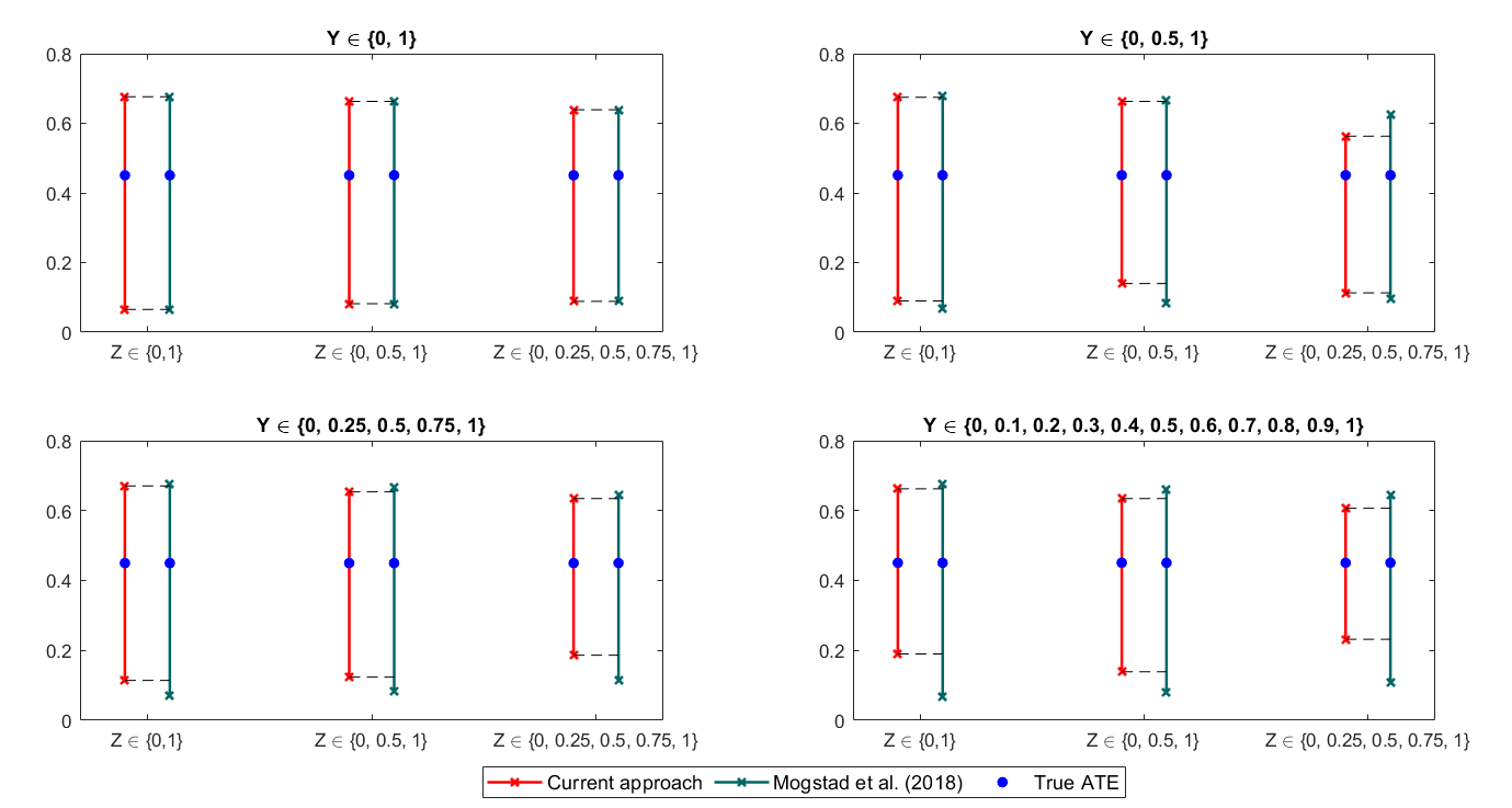
Figure 1: Full vs. Mean Independence: Bounds on ATE with Discrete $Z$ and $Y$

Figure 1 compares bounds that are calculated by using the current approach with those that are replicated by using Mogstad et al. (2018)’s approach. The first subfigure on the top-left shows that the bounds are identical between the two methods, because $Y$ is binary and thus full independence between $Y(d)$ and $Z$ is equivalent to mean independence. This equivalence is maintained no matter how many values $Z$ takes. In the next three subfigures, our bounds are tighter than Mogstad et al. (2018)’s as we expect. They show a pattern that, as $\mathcal{Y}$ contains more values, the improvement from the current approach is more substantial. This is because, as $Y$ takes more values, with greater degree, full independence contains richer structure than mean independence. Again, this pattern remains to hold regardless of the choice of $\mathcal{Z}$. It would also be interesting to investigate (i) the case with continuous $Y$ and (ii) the impact of $\mathcal{Z}$ when we move its endpoints further apart. They are explored in Section D.1 of the Appendix.

8.3 Bounds under Different Assumptions

8.3.1 ATE

Focusing on binary $Y$, Table 2 contains the bounds on the ATE under different assumptions, and these bounds are illustrated in Figure 2 and 3. The true ATE value is $0.15$, depicted as the solid red line in the figure. From 2, the worst-case bounds on the ATE with no additional assumptions (and without using variation from $W$) are $[-0.25,0.45]$. Since the mappings do not involve $W$, we have $|\mathcal{E}|=4$, and the linear programming is solved with $\dim(\theta)=\left|\mathcal{E}\right|\times\left|\mathcal{X}\right|\times(K+1)=4\times 2\times 51=408$.

For comparison, we calculate the bounds that incorporate the existence of $W$. We express the target parameters with mappings involving $W$ and use data distribution conditional on $W=0$ and $W=1$ as the constraints. With binary $W$, we have $|\mathcal{E}|=16$, which gives $\dim(\theta)=\left|\mathcal{E}\right|\times\left|\mathcal{X}\right|\times(K+1)=16\times 2\times 51=1,632$. The resulting bounds are depicted in the dotted greenish-blue line. When the variation from $W$ is used, the bounds on the ATE are $[-0.21,0.42]$, which is narrower than without using $W$. This result is consistent with our theoretical finding presented in Theorem 6.1 that $W$ can help tighten the bounds as long as it is a relevant variable. Nonetheless, these worst-case bounds are not that informative, e.g., they do not determine the sign of the ATE.

Next, we impose Assumption U⁰ without $W$ and with $W$. Under Assumption U⁰, the bounds on the ATE are tightened as we incorporate extra inequality constraints according to the direction of monotonicity. As mentioned in Section 6.1.1, the direction of monotonicity in Assumption U⁰ is determined by the LPs. We solve the LPs with different directions imposed, then choose the one with a feasible solution. This means that the corresponding direction of monotonicity is consistent with the DGP. Under Assumption U⁰, we obtain a bound $[0.05,0.45]$, which is narrower comparing with the worst-case bound. With $W$, under Assumption U⁰, the bounds become $[0.05,0.42]$. In Figure 2, these bounds under Assumptions U⁰ without and with $W$ are depicted as violet and green dashed lines, respectively. Both sets of bounds identify the sign of the ATE, consistent with the theoretical discussion. The improvement is mainly on the lower bounds and the upper bounds coincide with the corresponding worst-case upper bound without and with $W$. These improvements come from the ability to identify the sign under the uniformity assumptions.

Next, we impose the shape restrictions (Assumptions M and C). As discussed in Section 6.1.3, these assumptions can be easily incorporated in the linear programming by directly imposing inequality constraints on $\theta$. Under these assumptions (and the existence of $W$), the bounds on the ATE shrink to $[0.12,0.19]$, which is displayed with the pink line in Figure 2. We find that shape restrictions are powerful assumptions and yield narrower bounds compared to those with uniformity assumptions. They function differently in the linear programming: unlike the uniformity assumption, which maintains the ranking of individuals across counterfactual groups, shape restrictions directly control the MTR functions.

Table 2: Bounds on ATE under Various Assumptions

Assumptions	Lower Bound	Upper Bound	True Value
No Assumption	-0.25	0.45	0.15
Incorporating $W$	-0.21	0.42	0.15
Assumption U0	0.05	0.45	0.15
Incorporating $W$+Assumption U0	0.05	0.42	0.15
Incorporating $W$+Monotonicity+Concavity	0.12	0.19	0.15
Incorporating $W$+Assumption U∗	0.05	0.38	0.15

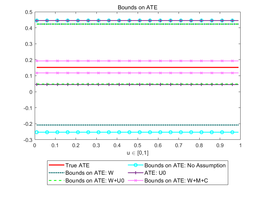
Figure 2: Bounds on the ATE under Different Assumptions

Figure 3 presents the results under Assumption U⁰, versus under Assumption U^∗ with existence of $W$. Under Assumption U^∗, the bounds become $[0.05,0.38]$. While their lower bounds coincide, Assumption U^∗ yields a lower upper bound compared to Assumption U⁰.

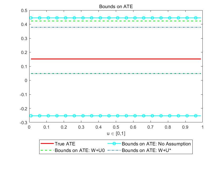
Figure 3: Bounds on the ATE under Different Assumptions

8.3.2 Generalized LATEs

Next, we construct bounds on the generalized LATEs. Again, we focus on binary $Y$. The original definition of the LATE is the ATE for compliers (C). Researchers may also have interests in other local treatment effects. We consider two other parameters—LATEs for always-takers (AT) and never-takers (NT). Figure 4 and 5 display the bounds on the LATE-AT, LATE-C, and LATE-NT under different assumptions. This analysis is analogous to that with the ATE. Since the covariate $X$ affects the decision of compliance, to avoid confusion in the definition of the compliance groups, we instead establish bounds on the LATEs conditional on $X$. We draw the conditional MTE functions with solid red lines in both panels as a reference.

The DGP implies constant MTE function, therefore, the LATE-AT, LATE-C and LATE-NT are all equivalent to true ATE, equaling to $0.33,0.23,0.13$ and $0.20,0.11,0.08$, conditional on $X=0$ and $X=1$ respectively. The feature that there exists no defiers in the DGP is known. When there is no defier, the LATE-C is point identified, which has an analytical expression of the two-stage least squares estimand. Therefore, even when we add the tuning parameters, the estimates remain very close to the true values throughout. And when we do not need tuning parameters to adjust the numerical errors or when the tuning parameters are very small, the linear programming yields point estimates as shown in Figure 4.

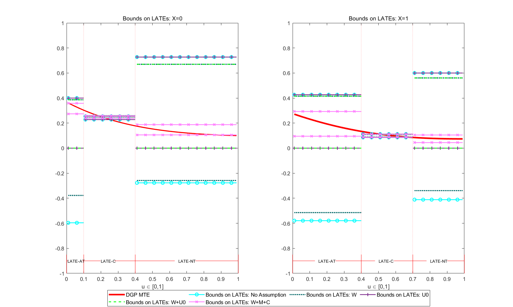
Figure 4: Bounds on the LATEs under Different Assumptions

For the LATE-AT and LATE-NT, as before, we first consider the worst-case bounds where the existence of $W$ is ignored versus where $W$ is taken into account. Without $W$, we get the bounds $[-0.60,0.40]$ and $[-0.28,0.73]$ on the LATE-AT and the LATE-NT conditional on $X=0$, and $[-0.58,0.43]$ and $[-0.41,0.60]$ conditional on $X=1$; with $W$, we get the bounds $[-0.38,0.39]$ and $[-0.26,0.67]$ on the LATE-AT and the LATE-NT conditional on $X=0$, and $[-0.51,0.42]$ and $[-0.34,0.56]$ conditional on $X=1$. Incorporating information from $W$ helps improve both the upper and lower bounds. Imposing Assumption U⁰ without $W$ helps to identify the sign by raising up the lower bound to $0$, for the LATEs; when considering the case with $W$, the pattern remains the same, but with a lower upper bound and a slightly improved lower bound above $0$. We then apply M and C with $W$ taking into account. The bounds on the LATE-AT and the LATE-NT turn to $[0.27,0.36]$ and $[0.11,0.19]$ conditional on $X=0$, and $[0.10,0.29]$ and $[0.04,0.11]$ conditional on $X=1$.

From Figure 5, under the Assumption U^∗, the bounds shrink to $[0,0.37]$ and $[0,0.53]$ conditional on $X=0$, and $[0,0.40]$ and $[0,0.55]$ conditional on $X=1$, comparing with the bounds under Assumption U⁰. The improvement is from complete order of 16 mapping types we have in this environment and is most significant for the never-taker LATE upper bound.

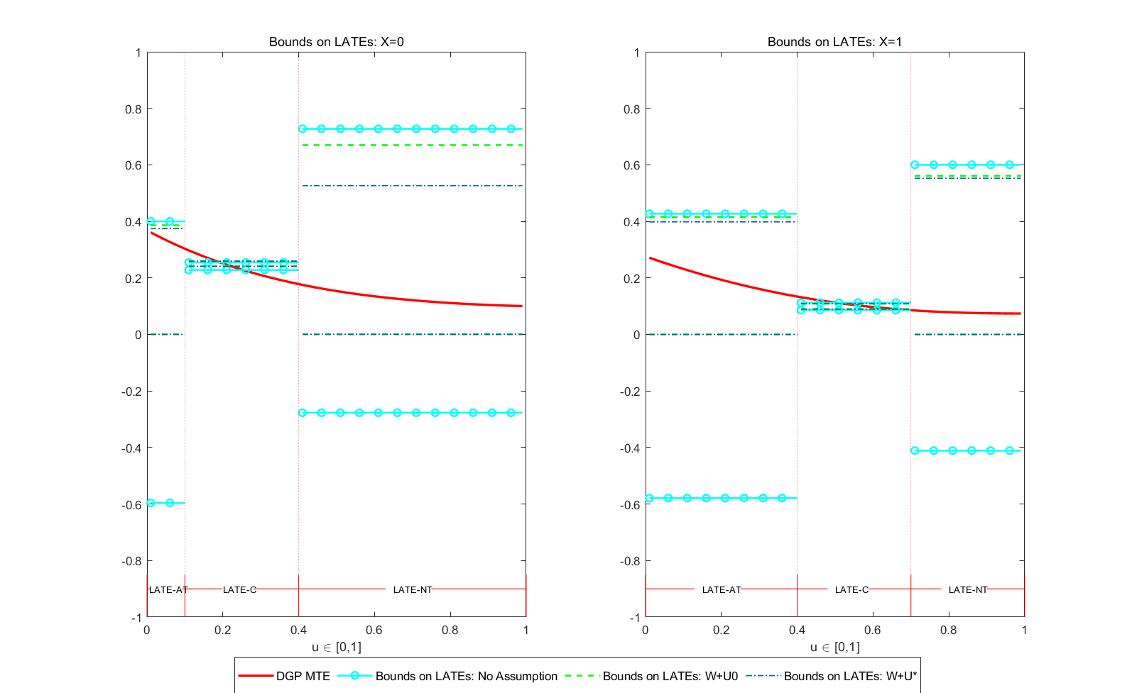
Figure 5: Bounds on the LATEs under Different Assumptions

8.4 The Choice of $K$

As a tuning parameter in the LP, we need to choose the order of Bernstein polynomials, $K$. In general, $K$ should be chosen based on the sample size and the smoothness of the function to be approximated, in our case, $q(\cdot)$. The choice of the sieve dimension or more generally, regularization parameters, is a difficult question (Chen (2007)) and developing data-driven procedure is a subject of on-going research in various nonparametric contexts of point identification; see, e.g., Chen and Christensen (2018) and Han (2020). In this partial identification setup, we propose the following heuristic and conservative approach, which is in spirit consistent with the very motivation of partial identification.

First, we do not want to claim any prior knowledge about the smoothness of $q(\cdot)$ because it is the distribution of a latent variable. Because $K$ determines the dimension of unknown parameter $\theta$ in the linear programming, the width of the bounds tends to increase with $K$. At the same time, the computational burden increases with $K$. One interesting numerical finding is that, when $K$ is sufficiently large, the increase of the width slows down and the bounds become stable. This suggests that we may be able to conservatively choose $K$ that acknowledges our lack of knowledge of the smoothness but, at the same time, produces a reasonable computational task for the linear programming.

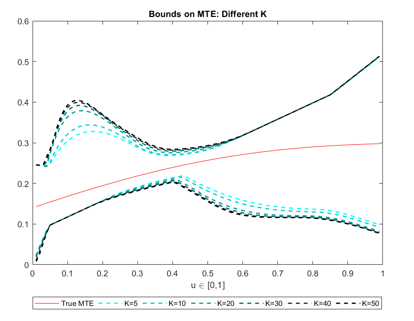
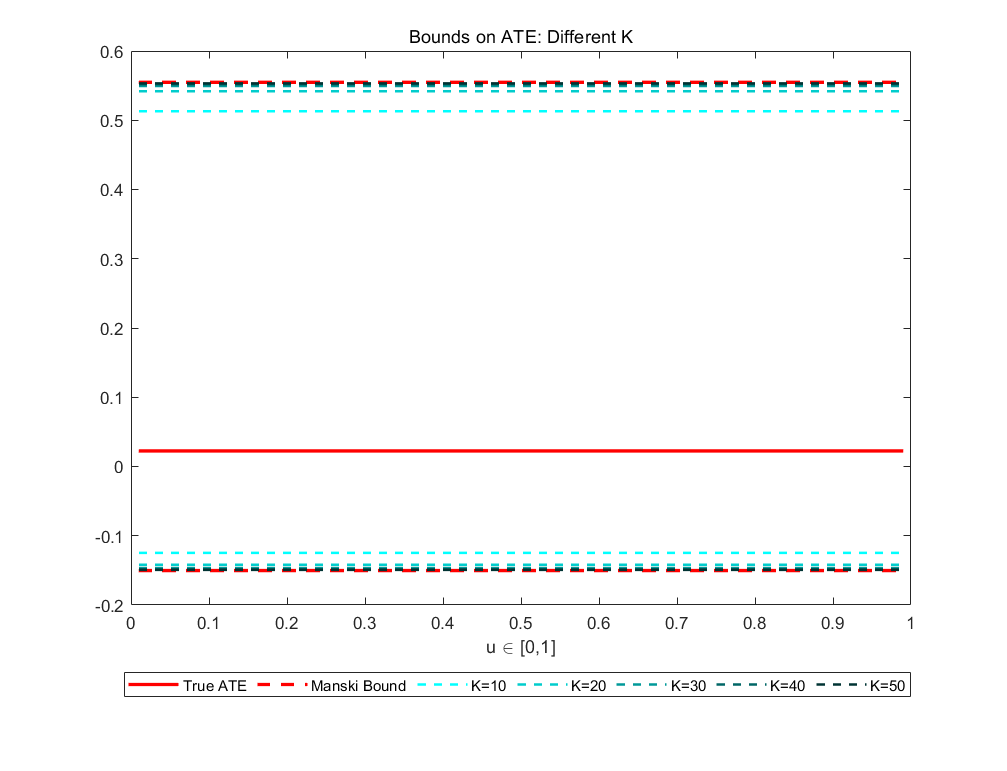
Figure 6: Bounds on MTE and ATE with Different $K$

To illustrate this point, we first consider the conditional MTE as the target parameter and show how its bounds change as $K$ increases. We consider the MTE because it is a fundamental parameter that generates other target parameters, and hence, it is important to understand the sensitivity of its bounds to $K$. The left panel of Figure 6 shows the evolution of the bounds on the MTE as $K$ grows. We use a DGP similar to the one described earlier. When $K=5$, the bounds are narrow. Although it may be tempting to choose this value of $K$, this attempt should be avoided as it may be subject to the misspecification of the true smoothness. When $K$ increases beyond $30$, the bounds start to converge and become stable. We choose $K=50$, and this is the choice we made in our previous numerical exercises.

To compare this converging pattern with a known benchmark, in the right panel of Figure 6, we depict the identified set for the ATE relative to Manski’s analytical bounds (Manski (1990)). We observe the identified set approaches to Manski’s bound as $K$ increases and it almost overlaps with Manski’s bounds when $K$ is around 50.

As discussed in Section B.2 in the Appendix, it is worth mentioning that the bounds on the MTE are pointwise sharp but not uniformly sharp. The graph for the MTE bounds are drawn by calculating the pointwise sharp bounds on MTE at each point of $u$ (after properly discretizing it) and then connecting them. Therefore, these bounds should not be viewed as uniformly sharp bounds. Nonetheless, this graph is still useful for the purpose of our illustration. Given the current DGP, we find that there are no uniformly sharp bounds for the MTE.

9 Empirical Application

It is widely recognized in the empirical literature that health insurance coverage can be an essential factor for the utilization of medical services (Hurd and McGarry (1997); Dunlop et al. (2002); Finkelstein et al. (2012); Taubman et al. (2014)). Prior studies on this topic typically make use of parametric econometric models for the analysis. In their application, Han and Lee (2019) relax this common approach by introducing a semiparametric bivariate probit model to measure the average effect of insurance coverage on patients’ medical visits. By applying our theoretical framework of partial identification, we further relax the parametric and semiparametric structures used in these studies. More importantly, we try to understand how much we can learn about the effect of insurance that is utilized through various counterfactual policies by learning the effect of different compliance groups.

We use the 2010 wave of the Medical Expenditure Panel Survey (MEPS) and focus on all the medical visits in January 2010. The sample is restricted to contain individuals aged between 25 and 64 and exclude those who had any kind of federal or state insurance in 2010. The outcome $Y$ is a binary variable indicating whether or not an individual has visited a doctor’s office; the treatment $D$ is whether an individual has private insurance. We choose whether a firm has multiple locations as the binary instrument $Z$. This IV reflects the size of the firm, and larger firms are more likely to provide fringe benefits, including health insurance. On the other hand, the number of branches of a firm does not directly affect employee decisions about medical visits. To justify the IV, self-employed individuals are excluded. For potentially endogenous covariates $X$, we include the age being 45 and older, gender, income above median. Lastly, for an exogenous covariate $W$, we use the percentage of workers who are provided with paid sick leave benefits within each industry. Following Han and Lee (2019), we assume $W$ satisfies Assumptions SEL_W(b) and EX_W(b), as $X$ is controlled. The rationale is the following: First, we assume $W$ is exogenous (conditional on covariates) arguably because it is determined by the employer or is in accordance with the local legislation and thus is not correlated with individual employee’s preferences. However, due to its nature, it can influence the employee’s health-related decisions, such as enrolling in an insurance program ($D$) or utilizing medical services ($Y$). We construct a categorical variable such that $W=0$ for less than median value of the pay sick leave provision, $W=1$ for above the median.

Table 3: Summary Statistics

	Variables	Mean	S.D	Min	Max
$Y$	Whether or not visit doctors	0.18	0.39	0	1
$D$	Whether or not have insurance	0.66	0.47	0	1
$Z$	Firm has multiple locations	0.68	0.47	0	1
$X$	Age above 45	0.41	0.49	0	1
	Gender	0.50	0.50	0	1
	Income above median	0.50	0.50	0	1
$W$	Pay sick leave provision	0.49	0.50	0	1
Number of observations = 7,555

First, as a benchmark, we report that the LATE-C estimate calculated via our linear programming approach is equal to a singleton of 0.05, which is in fact identical to the 2SLS estimate we separately calculate. In what follows, we extrapolate this LATE beyond the complier group to the ATE. The presence of covariates reduces the effective sample size and thus leads to larger sampling errors in estimating the $p$ of the $\infty$-LP ($\infty$-LP1)–($\infty$-LP3). This may create inconsistencies in the set of equality constraints ($\infty$-LP3), resulting in no feasible solution. This is in fact what happens in this application. To resolve this estimation problem, we introduce a slackness parameter $\kappa$ and modify ($\infty$-LP3) so that, with some slackness, it satisfies

$$||\hat{R}_{0}q-\hat{p}|| \leq\inf_{q\in\mathcal{Q}}||\hat{R}_{0}q-\hat{p}||+\kappa,$$ (9.1)

where $\hat{R}_{0}$ and $\hat{p}$ are estimates of $R_{0}$ and $p$. A similarly modified constraint can then be followed in the finite-dimensional LP after approximation, as well as by combining ($\infty$-LP4)–($\infty$-LP5). The appropriate value of $\kappa$ should depend on the sample size, the dimension of covariates, and the dimension of the unknown parameter $\theta$. To explain the latter, as $K$ increases, the dimension of $\theta$ (i.e., unknowns) increases, while the number of constraints (i.e., simultaneous equations for the unknowns) is fixed. Therefore, as $K$ increases, the chance that the LP does not have a feasible solution would decrease. Based on the method discussed in the previous section, we set $K=50$ in this application.

We calculate worst-case bounds on the ATE, as well as bounds after imposing Assumptions U⁰ and M and after using $W$. Under Assumption U⁰, the data rules out the possibility that $Y(0)>Y(1)$, indicating that individuals with private insurance are more likely to visit a doctor. Assumption M imposes that the MTR function is weakly increasing in $U=u$. Usually, $U$ is interpreted as the latent cost of obtaining treatment. Kowalski (2021) interpreted $U$ as eligibility in a similar setup for Medicaid insurance. The eligibility for Medicaid is related to income level and age. In our setup, because the treatment is having the private insurance, we interpret the eligibility as the health status, which is reflected in the premium. Interpreting $U$ as a latent cost (e.g., premium) of getting private insurance, Assumption M states that the chance of making a medical visit (with or without insurance) increases for those with higher cost. This is a reasonable assumption given that sicker individuals typically face higher insurance costs and also visit doctors more often. We choose the slackness parameter $\kappa$ to be consistently 0.01 under all assumptions for a comparable comparison.

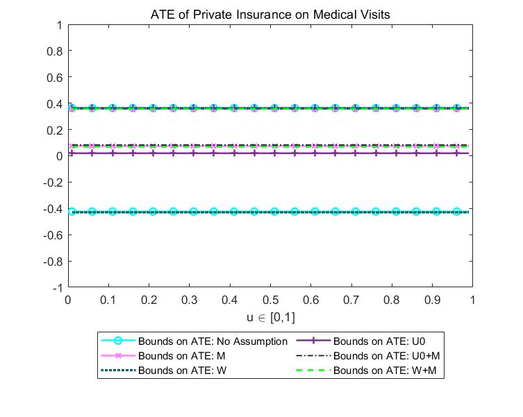
Figure 7: Bounds on the ATE of Private Insurance on Medical Visits

The bounds on the ATE are shown in Figure 7. The worst-case bound on the ATE equals $[-0.42,0.36]$. The bounds become $[0.02,0.36]$ under Assumption U⁰ and $[0.07,0.36]$ under Assumption M. It is interesting to note that the identifying power of the uniformity and the shape restriction is similar in this example. When both Assumption U⁰ and Assumption M are imposed, the bounds are further tightened to $[0.08,0.36]$, although not substantially, indicating that the two assumptions are complementary. However, we do not see gain from incorporating $W$ in this case.

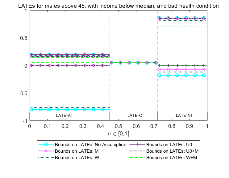
Figure 8: Bounds on the generalized LATEs of Private Insurance on Medical Visits for Male Above 45, with Income Below Median

Table 4: Estimated Bounds on generalized LATEs for Males Above 45, with Income Below Median

	No Assumption	Assumption U0	M	Assumption U0+M	W	M+W
LATE-AT	[-0.80,0.19]	[0,0.19]	[0,0.16]	[0,0.16]	[-0.77,0.18]	[0.05,0.14]
LATE-C	0.05	0.05	0.05	0.05	0.05	0.05
LATE-NT	[-0.18,0.86]	[0,0.86]	[-0.07,0.85]	[0,0.85]	[-0.12,0.81]	[0,0.70]
Slackness $\kappa$	0.01	0.01	0.01	0.01	0.01	0.01
Number of observations = 7,555

Next, we consider the always-taker, complier, and never-taker LATEs. We consider these generalized LATEs conditional on $X=x$. Specifically, we focus on the treatment effects for males above age 45, with income below the median. The results are shown in Table 4 and depicted in Figure 8. The LATE-C is analytically calculated via TSLS. For the LATE-AT and LATE-NT, Assumption U⁰ identifies the sign of the effects, and Assumption M nearly identifies it. Using the variation in $W$ mostly improves the bounds compared to the ones without it. From the results we can conclude that, for a range of identifying assumptions, the private insurance tends to have a large effect on medical visits for never-takers, that is, people who face higher insurance cost. For example, for all the cases, the upper bound on the effect (i.e., the most optimistic scenario) is much larger for the never-takers than the always-takers. Under Assumption W or no assumption, the lower bounds (i.e., the most pessimistic scenario) shows a similar pattern. This suggests a policy implication that lowering the cost of private insurance may be important, because high costs may hinder those with the most need from receiving enough medical services.

Appendix A Examples of the Target Parameters

Table 5 contains the list of target parameters.

Target Parameters	Expressions	Ranges of $u$	Weights
			$w_{d}(u,z,x)$
Average Treatment Effect	$E[Y(1)-Y(0)]$	$[0,1]$	$1$
(ATE)
LATE for Compliers	$E\left\{Y(1)-Y(0)|u\in\left[P(z_{0},x),P(z_{1},x)\right]\right\}$	$[P(z_{0},x),P(z_{1},x)]$	$\frac{1\left(u\in[P(z_{0},x),P(z_{1},x)]\right)}{P(z_{1},x)-P(z_{0},x)}$
(LATE-C) given $x\in\mathcal{X}$
LATE for Always-Takers	$E\left\{Y(1)-Y(0)|u\in\left[0,P(z_{0},x)\right]\right\}$	$[0,P(z_{0},x)]$	$\frac{1\left(u\in[0,P(z_{0},x)]\right)}{P(z_{0},x)}$
(LATE-AT) given $x\in\mathcal{X}$
LATE for Never-Takers	$E\left\{Y(1)-Y(0)|u\in\left[P(z_{1},x),1\right]\right\}$	$[P(z_{1},x),1]$	$\frac{1\left(u\in[P(z_{1},x),1]\right)}{1-P(z_{1},x)}$
(LATE-NT) given $x\in\mathcal{X}$
LATE for $[\underline{u},\overline{u}]$	$E[Y(1)-Y(0)|u\in[\underline{u},\overline{u}]]$	$\left[P(z_{0},x),P(z_{1},x)\right]$	$\frac{1\left(u\in[\underline{u},\overline{u}]\right)}{\overline{u}-\underline{u}}$
Marginal Treatment Effect	$E[Y(1)-Y(0)|u^{\prime}]$	$u^{\prime}$	$1(u=u^{\prime})$
(MTE)∗
Policy Relevant Treatment Effect	$\frac{E(Y^{\prime})-E(Y)}{E(D^{\prime})-E(D)}$	$[0,1]$	$\frac{\Pr\left[u\leq P^{\prime}(z^{\prime})\right]-\Pr\left[u\leq P^{\prime}(z)\right]}{E\left[P(Z^{\prime})\right]-E\left[P(Z)\right]}$
(PRTE) for a new policy $(P^{\prime},Z^{\prime})$

* The MTE uses the Dirac measure at $u^{\prime}$, while the other target parameters use the Lebesgue measure on $[0,1]$.

Table 5: Examples of the Target Parameters

Appendix B Further Discussions

B.1 Rescaling of Linear Programs

Let $B\theta=p$ represents the constraints (LP3) in the LP (LP1)–(LP3). In practice, the matrix $B$ has the number of columns that grows with $K$. An important consequence is that, when $K$ is large, the entries of $B$ (i.e., constraint coefficients) take values of very different orders of magnitude; some coefficients are too small and some are too large. In this case, many optimization algorithms do not work properly because, to address the issue, they arbitrarily drop coefficients with small values (e.g., GUROBI drops coefficients that are less than $10^{-13}$). This may arbitrarily change the bounds we obtain. In this section, we propose a rescaling method to address this problem.

To better understand the rescaling strategy, we first express the original LP (LP1)–(LP3) in terms of matrices:

$$\max_{\theta\in\Theta_{K}}A\theta$$

subject to

$$B\theta=p.$$

Here, $\theta$ is defined as a vector of unknown parameters $\{\theta_{k}^{e,x}\}_{k,e,x}$ and $\Theta_{K}$ is redefined as

$$\Theta_{K}\equiv\left\{\theta:M\theta=\boldsymbol{1},\theta\geq\boldsymbol{0}\right\},$$

where $M$ is a weight matrix corresponding to $\sum_{e\in\mathcal{E}}\theta_{k}^{e,x}=1$ $\forall(k,x)$, $\boldsymbol{1}$ is a column vector of ones, and $\boldsymbol{0}$ is a zero vector.

Because the Bernstein polynomials are only used in generating the coefficients in the equality restrictions from the data, we focus on rescaling of this constraint. Suppose the dimension of $B$ is $m\times n$ with $m<n$. First, we show that $B$ has full rank of $m$ in our setting. To prove this, we need to understand the structure of $B$. The number of columns of $B$ is determined by the size of $\mathcal{E}$ and the order of polynomials $K$. The number of rows of $B$ is determined by the dimension of $p$. We consider an example with binary $(Y,Z,W)$ for illustration. Since $(D,W)$ are binary, $\left|\mathcal{E}\right|=16$ and $B$ takes the form of the following:

$$\begin{array}[]{ccccccccccccccccc}e=&1&2&3&4&5&6&7&8&9&10&11&12&13&14&15&16\\ Z=0,D=0,W=0&&\text{{\char 96\relax}}&&\text{{\char 96\relax}}&&\text{{\char 96\relax}}&&\text{{\char 96\relax}}&&\text{{\char 96\relax}}&&\text{{\char 96\relax}}&&\text{{\char 96\relax}}&&\text{{\char 96\relax}}\\ Z=1,D=0,W=0&&\text{{\char 96\relax}}&&\text{{\char 96\relax}}&&\text{{\char 96\relax}}&&\text{{\char 96\relax}}&&\text{{\char 96\relax}}&&\text{{\char 96\relax}}&&\text{{\char 96\relax}}&&\text{{\char 96\relax}}\\ Z=0,D=1,W=0&&&&&\text{{\char 96\relax}}&\text{{\char 96\relax}}&\text{{\char 96\relax}}&\text{{\char 96\relax}}&&&&&\text{{\char 96\relax}}&\text{{\char 96\relax}}&\text{{\char 96\relax}}&\text{{\char 96\relax}}\\ Z=1,D=1,W=0&&&&&\text{{\char 96\relax}}&\text{{\char 96\relax}}&\text{{\char 96\relax}}&\text{{\char 96\relax}}&&&&&\text{{\char 96\relax}}&\text{{\char 96\relax}}&\text{{\char 96\relax}}&\text{{\char 96\relax}}\\ Z=0,D=0,W=1&&&\text{{\char 96\relax}}&\text{{\char 96\relax}}&&&\text{{\char 96\relax}}&\text{{\char 96\relax}}&&&\text{{\char 96\relax}}&\text{{\char 96\relax}}&&&\text{{\char 96\relax}}&\text{{\char 96\relax}}\\ Z=1,D=0,W=1&&&\text{{\char 96\relax}}&\text{{\char 96\relax}}&&&\text{{\char 96\relax}}&\text{{\char 96\relax}}&&&\text{{\char 96\relax}}&\text{{\char 96\relax}}&&&\text{{\char 96\relax}}&\text{{\char 96\relax}}\\ Z=0,D=1,W=1&&&&&&&&&\text{{\char 96\relax}}&\text{{\char 96\relax}}&\text{{\char 96\relax}}&\text{{\char 96\relax}}&\text{{\char 96\relax}}&\text{{\char 96\relax}}&\text{{\char 96\relax}}&\text{{\char 96\relax}}\\ Z=1,D=1,W=1&&&&&&&&&\text{{\char 96\relax}}&\text{{\char 96\relax}}&\text{{\char 96\relax}}&\text{{\char 96\relax}}&\text{{\char 96\relax}}&\text{{\char 96\relax}}&\text{{\char 96\relax}}&\text{{\char 96\relax}}\end{array}$$

The square represents a vector of coefficients corresponding to $\theta$’s used in approximating the mapping types, and the blank represents a zero vector. By construction, each entry in matrix $B$ is equivalent to $\int_{\mathcal{U}_{z,x}^{d}}b_{k,K}(u)du$ such that the product of $B$ and $\theta$ is equal to the data distribution. From the matrix form above, we can guarantee that $B$ has full row rank if, for given $(d,w)$, the row representing $Z=0$ cannot be a constant multiplication of the row representing $Z=1$.

Lemma B.1.

Suppose $Z\in\{z_{1},z_{2}\}$ is a binary IV. Assume that $P(z_{1}),P(z_{2})\in(0,1)$ and $P(z_{1})\neq P(z_{2})$. For $k=0,1,...,K$, define $f(k)=\frac{\int_{0}^{P(z_{1})}b_{k,K}(u)du}{\int_{0}^{P(z_{2})}b_{k,K}(u)du}$. Then, $f(k)$ is not a constant function, and thus $B$ has full row rank.

The proof of this lemma appears below. Our goal is to rescale the coefficient matrix $B$ into a new matrix $\tilde{B}$ such that its entries have balanced orders of magnitude. The most intuitive choice of $\tilde{B}$ is the fully reduced form of $B$. Note $B$ usually has more rows than columns (otherwise, we achieve point identification), therefore, the fully reduced form of $B$ would take the form of

$$\tilde{B}=\left[I,\boldsymbol{0}\right],$$

where $I$ is the identity matrix of rank $m$, and $\boldsymbol{0}$ is a zero matrix with dimension $m\times(n-m)$. The next step is to find a transformation matrix $X$ such that $BX=\tilde{B}$, so that we can rewrite the optimization problem as

$$\max_{\tilde{\theta}\in\tilde{\Theta}_{K}}\tilde{A}\tilde{\theta}$$

subject to

$$\tilde{B}\tilde{\theta}=p,$$

where $\tilde{\theta}=X^{-1}\theta$, $\tilde{A}=AX$, and $\tilde{\Theta}_{K}\equiv\left\{\tilde{\theta}:MX\tilde{\theta}=\boldsymbol{1},X\tilde{\theta}\geq\boldsymbol{0}\right\}$.

We propose a simple algorithm to find a full rank $X$. Since $B$ is the column-reduced form of $B$, $X$ can be viewed as the matrix of elementary operation used to reach the reduced form. To construct $X$, we first use the transposed matrix $B^{\prime}$ and apply to it Gauss-Jordan elimination with partial pivoting to achieve a row-reduced form. We apply the exactly same procedure to an identity matrix $I$ with dimension $n\times n$. Then, the transpose of the resulting matrix becomes $X$. Because simple row operations preserve the rank, $X$ is guaranteed to have full rank. Note that there may exist multiple solutions of $X$, which essentially makes this procedure computationally easier than solving an LP.

B.2 Pointwise and Uniform Sharp Bounds on MTE

In Section 2, we provided some examples of target parameters. The building block for these parameters is the MTE, $m_{1}(u)-m_{0}(u)$ (suppressing $w$ and $x$). Heckman and Vytlacil (2005) show why this fundamental parameter can be of independent interest. Unlike other target parameters proposed here, we may want to recover the MTE as a function of $u$ (besides evaluating it at fixed $u$). In this section, we discuss the subtle issue of pointwise and uniform sharp bounds on $\tau_{MTE}(u)\equiv m_{1}(u)-m_{0}(u)$ as a function of $u$.

For simplicity, suppress $W$ and $X$ and redefine $\epsilon\equiv(Y(0),Y(1))$ and $e\equiv(y(0),y(1))$. Recall $q(u)\equiv\{q(e|u)\}_{e\in\mathcal{\mathcal{E}}}$ and $\mathcal{Q}\equiv\{q(\cdot):\sum_{e}q(e|u)=1\,\forall u\text{ and }q(e|u)\geq 0\,\forall(e,u)\}$. Let $\mathcal{M}$ be the set of MTE functions, i.e.,

$$\mathcal{M}\equiv\Big{\{}m_{1}(\cdot)-m_{0}(\cdot):m_{d}(\cdot)=\sum_{e\in\mathcal{E}:y(d)=1}q(e|\cdot)\text{ }\forall d\in\{0,1\}\text{ for }q(\cdot)\in\mathcal{Q}\Big{\}}.$$

The bounds on $\tau_{MTE}\in\mathcal{M}$ in the $\infty$-LP are given by using a Dirac delta function as a weight. Therefore, given evaluation point $u\in[0,1]$, ($\infty$-LP1)–($\infty$-LP3) can be simplified as follows, defining the upper and lower bounds $\overline{\tau}(u)$ and $\underline{\tau}(u)$ (that are explicit about the evaluation point) on $\tau_{MTE}(u)$:

$$\overline{\tau}(u) =\sup_{q\in\mathcal{Q}}\sum_{e\in\mathcal{E}:y(1)=1}q(e|u)-\sum_{e\in\mathcal{E}:y(0)=1}q(e|u)$$ (B.1)

$$\underline{\tau}(u) =\inf_{q\in\mathcal{Q}}\sum_{e\in\mathcal{E}:y(1)=1}q(e|u)-\sum_{e\in\mathcal{E}:y(0)=1}q(e|u)$$ (B.2)

subject to

$$\sum_{e:y(d)=1}\int_{\mathcal{U}_{z}^{d}}q(e|\tilde{u})d\tilde{u} =p(1,d|z)\qquad\forall(d,z)\in\{0,1\}\times\mathcal{Z}.$$ (B.3)

Then, for any fixed $u\in[0,1]$,

$$\underline{\tau}(u) \leq\tau_{MTE}(u)\leq\overline{\tau}(u).$$

We argue that these bounds are pointwise sharp but not necessarily uniformly sharp for $\tau_{MTE}(\cdot)$.

Definition B.1 (Pointwise Sharpness).

$\overline{\tau}(\cdot)$ and $\underline{\tau}(\cdot)$ are pointwise sharp if, for any $\bar{u}\in[0,1]$, there exist $\overline{\tau}_{MTE,\bar{u}},\underline{\tau}_{MTE,\bar{u}}\in\mathcal{M}$ such that $\overline{\tau}(\bar{u})=\overline{\tau}_{MTE,\bar{u}}(\bar{u})$ and $\underline{\tau}(\bar{u})=\underline{\tau}_{MTE,\bar{u}}(\bar{u})$.

Theorem B.1.

$\overline{\tau}(\cdot)$ and $\underline{\tau}(\cdot)$ are pointwise sharp bounds on $\tau_{MTE}(\cdot)$.

The proofs of this and other theorems appear later. Note that pointwise bounds will maintain some properties of an MTE function, but not all. For uniform sharpness, $\overline{\tau}(\cdot)$ and $\underline{\tau}(\cdot)$ themselves have to be MTE functions on $[0,1]$, i.e., $\overline{\tau}(\cdot)$ and $\underline{\tau}(\cdot)$ should be elements in $\mathcal{M}$.

Definition B.2 (Uniform Sharpness).

$\overline{\tau}(\cdot)$ and $\underline{\tau}(\cdot)$ are uniformly sharp if $\overline{\tau}(\cdot),\underline{\tau}(\cdot)\in\mathcal{M}$.

The following theorem is almost immediate.

Theorem B.2.

$\overline{\tau}(\cdot)$ is uniformly sharp if and only if there exists $q^{*}(\cdot)\in\mathcal{Q}$ such that $q^{*}(\cdot)$ is in the feasible set and $\overline{\tau}(u)=\sum_{e\in\mathcal{E}:y(1)=1}q^{*}(e|u)-\sum_{e\in\mathcal{E}:y(0)=1}q^{*}(e|u)$ for all $u\in[0,1]$. Similarly, $\underline{\tau}(\cdot)$ is uniformly sharp if and only if there exists $q^{\dagger}(\cdot)\in\mathcal{Q}$ such that $q^{\dagger}(\cdot)$ is in the feasible set and $\underline{\tau}(u)=\sum_{e\in\mathcal{E}:y(1)=1}q^{\dagger}(e|u)-\sum_{e\in\mathcal{E}:y(0)=1}q^{\dagger}(e|u)$ for all $u\in[0,1]$.

The following is a more useful result that relates pointwise bounds with uniform bounds. For each $\bar{u}$, let $q_{\bar{u}}^{*}(\cdot)$ and $q_{\bar{u}}^{\dagger}(\cdot)$ be the pointwise maximizer and minimizer of (B.1)–(B.3), respectively.

Corollary B.1.

$\overline{\tau}(\cdot)$ is uniformly sharp if and only if there exists $q^{*}(\cdot)\in\mathcal{Q}$ such that $q^{*}(\cdot)$ is in the feasible set and $q_{\bar{u}}^{*}(\bar{u})=q^{*}(\bar{u})$ for all $\bar{u}\in[0,1]$. Also, $\underline{\tau}(u)$ is uniformly sharp if and only if there exists $q^{\dagger}(\cdot)\in\mathcal{Q}$ such that $q^{\dagger}(\cdot)$ is in the feasible set and $q_{\bar{u}}^{\dagger}(\bar{u})=q^{\dagger}(\bar{u})$ for all $\bar{u}\in[0,1]$.

Based on the Bernstein approximation we introduce, this corollary implies that for a uniform upper bound to exist, there should exist a common maximizer $\theta^{*}$ such that $\theta^{*}$ is in the feasible set of the LP and $\overline{\tau}(u)=\sum_{k\in\mathcal{K}}\Big{\{}\sum_{e\in\mathcal{E}:y(1)=1}\theta_{k}^{e*}b_{k}(u)-\sum_{e\in\mathcal{E}:y(0)=1}\theta_{k}^{e*}b_{k}(u)\Big{\}}$ for all $u$. In other words, if $\theta_{\bar{u}}^{*}$ is the maximizer of the LP for given $\bar{u}$, then there should exist $\theta^{*}$ in the feasible set such that $\theta_{\bar{u}}^{*}=\theta^{*}$ for all $\bar{u}\in[0,1]$. Since this condition will not generally hold, uniformly sharp bounds on the MTE may not exist. The condition can be verified in practice by implementing the LP in a finite grid of $u$ in $[0,1]$ and checking whether $\theta_{u}^{*}$ is constant for all values in the grid.

The discussion of this section extends to the case with continuous $Y$ by analogously defining the set of MTE functions generated by $\tilde{\mathcal{Q}}$. One implication of uniform sharpness is that $\overline{\tau}(\cdot)$ and $\underline{\tau}(\cdot)$ should be consistent with the CDF properties of $\tilde{q}(e|u)$ embedded in $\tilde{\mathcal{Q}}$.

B.3 Linear Programming with Continuous $X$

Suppose $X$ is a vector of continuously distributed covariates and assume $\mathcal{X}=[0,1]^{d_{X}}$ without loss of generality. Let $q(u,x)\equiv\{q(e|u,x)\}_{e\in\mathcal{\mathcal{E}}}$ and $p(x)\equiv\{p(1,d|z,w,x)\}_{d,z,w}$. Recall that $R_{\omega}:\mathcal{Q}\rightarrow\mathbb{R}$ and $R:\mathcal{Q}\rightarrow\mathbb{R}^{d_{p}}$ are the linear operators of $q(\cdot)$ where $d_{p}$ is the dimension of $p$. Consider the following LP:

$$\overline{\tau}= \sup_{q\in\mathcal{Q}}R_{\omega}q,$$ (B.4)

$$\underline{\tau}= \inf_{q\in\mathcal{Q}}R_{\omega}q,$$ (B.5)

$$s.t.\quad(Rq)(x)=p(x)\qquad\text{for all }x\in\mathcal{X},$$ (B.6)

where $(Rq)(x)=p(x)$ emphasizes the dependence on $x$, and thus represents infinitely many constraints. Therefore, this LP is infinite dimensional because of both the decision variable and the constraints.

Now, for the sieve space of $\mathcal{Q}$, we consider

$$\bar{\mathcal{Q}}_{K} \equiv\left\{\Big{\{}\sum_{k=1}^{K}\theta_{k}^{e}b_{k}(u,x)\Big{\}}_{e\in\mathcal{E}}:\sum_{e\in\mathcal{E}}\theta_{k}^{e}=1\text{ and }\theta_{k}^{e}\geq 0\text{ }\forall(e,k)\right\}\subseteq\mathcal{Q},$$ (B.7)

where $b_{k}(u,x)$ is a bivariate Bernstein polynomial and $\mathcal{K}\equiv\{1,...,K\}$. Then, for $q\in\bar{\mathcal{Q}}_{K}$

$$E[\tau_{d}(Z,W,X)] =E\left[\sum_{e:y(d,W)=1}\sum_{k\in\mathcal{K}}\theta_{k}^{e}\int b_{k}(u,X)\omega_{d}(u,Z,X)du\right]$$

$$\equiv\sum_{w\in\mathcal{W}}\sum_{e:y(d,w)=1}\sum_{k\in\mathcal{K}}\theta_{k}^{e}\tilde{\gamma}_{k}^{d}(w),$$ (B.8)

where $\tilde{\gamma}_{k}^{d}(w)\equiv E\left[\sum_{z\in\{0,1\}}p(z,w|X)\int b_{k}(u,X)\omega_{d}(u,z,X)du\right]$ with $p(z,w|x)\equiv\Pr[Z=z,W=w|X=x]$. Also,

$$p(1,d|z,w,x) =\sum_{e:y(d,w)=1}\sum_{k\in\mathcal{K}}\theta_{k}^{e}\int_{\mathcal{U}_{z,x}^{d}}b_{k}(u,x)du$$

$$\equiv\sum_{e:y(d,w)=1}\sum_{k\in\mathcal{K}}\theta_{k}^{e}\tilde{\delta}_{k}^{d}(z,x),$$ (B.9)

where $\tilde{\delta}_{k}^{d}(z,x)\equiv\int_{\mathcal{U}_{z,x}^{d}}b_{k}(u,x)du$. To deal with this infinite dimensional constraints (with respect to $x$), we proceed as follows. For any measurable function $h:\mathcal{X}\rightarrow\mathbb{R}$, $E\left|h(X)\right|=0$ if and only if $h(x)=0$ almost everywhere in $\mathcal{X}$. Therefore, the equality restriction (B.9) can be replaced by

$$E\left|\sum_{e:y(d,w)=1}\sum_{k\in\mathcal{K}}\theta_{k}^{e}\tilde{\delta}_{k}^{d}(z,X)-p(1,d|z,w,X)\right| =0$$

for all $(d,z,w)\in\{0,1\}\times\mathcal{Z}\times\mathcal{W}$. Let $\tilde{\theta}\equiv\{\theta_{k}^{e}\}_{(e,k)\in\mathcal{E}\times\mathcal{K}}$ and let

$$\tilde{\Theta}_{K} \equiv\left\{\tilde{\theta}:\sum_{e\in\mathcal{E}}\theta_{k}^{e}=1\text{ and }\theta_{k}^{e}\geq 0\text{ }\forall(e,k)\in\mathcal{E}\times\mathcal{K}\right\}.$$

Then, we can formulate the following finite-dimensional LP:

$$\overline{\tau}_{K} =\max_{\theta\in\Theta_{K}}\sum_{(k,w)\in\mathcal{K}\times\mathcal{W}}\Big{\{}\sum_{e:y(1,w)=1}\theta_{k}^{e}\tilde{\gamma}_{k}^{1}(w)-\sum_{e:y(0,w)=1}\theta_{k}^{e}\tilde{\gamma}_{k}^{0}(w)\Big{\}}$$ (B.10)

$$\underline{\tau}_{K} =\min_{\theta\in\Theta_{K}}\sum_{(k,w)\in\mathcal{K}\times\mathcal{W}}\Big{\{}\sum_{e:y(1,w)=1}\theta_{k}^{e}\tilde{\gamma}_{k}^{1}(w)-\sum_{e:y(0,w)=1}\theta_{k}^{e}\tilde{\gamma}_{k}^{0}(w)\Big{\}}$$ (B.11)

subject to

$$E\left|\sum_{e:y(d,w)=1}\sum_{k\in\mathcal{K}}\theta_{k}^{e}\tilde{\delta}_{k}^{d}(z,X)-p(1,d|z,w,X)\right| =0\qquad\forall(d,z,w)\in\{0,1\}\times\mathcal{Z}\times\mathcal{W}.$$ (B.12)

Later, we want to introduce additional constraints from some identifying assumptions:

$$R_{1}q =a_{1},$$ (B.13)

$$R_{2}q \leq a_{2}.$$ (B.14)

For the equality restrictions, we can use the same approach that transforms (B.6). For the inequality restrictions (B.14), we can allow any identifying assumptions for which $R_{2}$ is a matrix rather than an operator:

Assumption MAT.

$R_{2}$ is a $\dim(a_{2})\times\dim(q)$ matrix.

Assumptions M and C and the unconditional version of Assumption MTS satisfy this condition.

B.4 Estimation and Inference

Although the paper’s main focus is identification, we briefly discuss estimation and inference. Assume a random sample of $\{Y_{i},D_{i},Z_{i},W_{i},X_{i}\}_{i=1}^{N}$. The estimation of the bounds characterized by the LP (LP1)–(LP3) is straightforward by replacing the population objects $(\gamma_{k}^{d},\delta_{k}^{d},p)$ with their sample counterparts $(\hat{\gamma}_{k}^{d},\hat{\delta}_{k}^{d},\hat{p})$. To account for the statistical error arising from estimation based on the finite sample, we replace $\infty$-LP3 with a tuned constraint:

$$||\hat{R}_{0}q-\hat{p}||\leq\inf_{q\in\mathcal{Q}}||\hat{R}_{0}q-\hat{p}||+\kappa.$$

Here $\kappa$ is a tuning parameter selected by the researchers. In the finite-dimensional LP, to be more specific, we apply the Euclidean norm and replace (LP3) by

$$\sqrt{\sum_{z,w,x}\left(\sum_{e:y(d,w)=1}\sum_{k\in\mathcal{K}}\theta_{k}^{e,x}\hat{\delta}_{k}^{d}(z,x)-\hat{p}(1,d|z,w,x)\right)^{2}}\leq$$

$$\;\;\;\;\;\;\;\;\;\;\;\;\;\;\;\;\;\;\;\;\;\;\;\;\;\;\;\;\;\;\;\;\;\;\;\;\;\;\;\inf_{\theta\in\Theta_{k}}\sqrt{\sum_{z,w,x}\left(\sum_{e:y(d,w)=1}\sum_{k\in\mathcal{K}}\theta_{k}^{e,x}\hat{\delta}_{k}^{d}(z,x)-\hat{p}(1,d|z,w,x)\right)^{2}}+\kappa.$$

With continuous $Y$ in (7.6)–(7.8), we replace (7.8) with (a slack version of) its sample counterparts:

$$\frac{1}{N}\sum_{i=1}^{N}\left|\sum_{\boldsymbol{k}\in\mathcal{K}^{5}}\theta_{\boldsymbol{k}}^{x}\hat{\sigma}_{\boldsymbol{k}}^{d}(Y_{i},Z_{i},X_{i})-\hat{\pi}(Y_{i},d|Z_{i},W_{i},X_{i})\right| \leq\eta,$$

where $\hat{\pi}(y,d|z,w,x)$ is some preliminary estimate of $\pi(y,d|z,w,x)$ and $\eta$ is another slackness parameter. Since $\eta$ takes into account the error from the finite sample, there is no need to introduce an additional tuning parameter to account for the estimation error. A similar idea applies to the case with continuous $X$ in (B.10)–(B.12).

It is important to construct a confidence set for our target parameter or its bounds in order to account for the sampling variation in measuring treatment effectiveness. It will also be interesting to develop a procedure to conduct a specification test for the identifying assumptions discussed in Section 6. The problem of statistical inference when the identified set is constructed via linear programming has been studied in, e.g., Deb et al. (2023), Mogstad et al. (2018), Hsieh et al. (2022), Torgovitsky (2019a), and fang2023inference. Among these papers, Mogstad et al. (2018)’s setting is closest to our setting with discrete variables, and their inference procedure can be directly adapted to our problem. Instead of repeating their result here, we only briefly discuss the procedure.

Recall $q(u)\equiv\{q(e|u,x)\}_{e\in\mathcal{\mathcal{E}},x\in\mathcal{X}}$ is the latent distribution and $p\equiv\{p(1,d|z,x)\}_{d,z,x}$ is the distribution of the data, and $R_{\omega}$, $R_{0}$, $R_{1}$, and $R_{2}$ denote the linear operators of $q(\cdot)$ that correspond to the target and constraints. Consider the following hypotheses:

$$H_{0}: p\in\mathcal{P}_{0},\qquad H_{1}:p\in\mathcal{P}\backslash\mathcal{P}_{0},$$

where

$$\mathcal{P}_{0} \equiv\{p\in\mathcal{P}:Rq=a\text{ for some }q\in\mathcal{Q}\}$$

and

$$R \equiv(R_{\omega}^{\prime},R_{0}^{\prime},R_{1}^{\prime},R_{2}^{\prime})^{\prime},$$

$$a \equiv(\tau,p^{\prime},a_{1}^{\prime},a_{2}^{\prime})^{\prime}.$$

Suppose $\hat{R}$ and $\hat{a}$ are sample counterparts of $R$ and $a$. Then, a minimum distance test statistic can be constructed as

$$T_{N}(\tau) \equiv\inf_{q\in\mathcal{Q}_{K}}\sqrt{N}\left\|\hat{R}q-\hat{a}\right\|.$$

Similar to Mogstad et al. (2017), $T_{N}(\tau)$ is the solution to a convex optimization problem that can be reformulated as an LP using duality. A $(1-\alpha)$-confidence set for the target parameter $\tau$ can be constructed by inverting the test:

$$CS_{1-\alpha} \equiv\{\tau:T_{N}(\tau)\leq\hat{c}_{1-\alpha}\}$$

where $\hat{c}_{1-\alpha}$ is the critical value for the test. The resulting object is of independent interest, and it can further be used to conduct specification tests. The large sample theory for $T_{N}(\tau)$, as well as a bootstrap procedure to calculate $\hat{c}_{1-\alpha}$, will directly follow according to Mogstad et al. (2017), which is omitted for succinctness.

When $Y$ or $X$ is continuously distributed, then the resulting LP is semi-infinite dimensional. In this case, the inference procedure by Chernozhukov et al. (2013) may be applied. In this case, the estimation of the bounds can be conducted within the framework.

Appendix C Proofs

C.1 Proof of Lemma 3.1

Fix $(d,z,w,x)$. By $\sum_{e\in\mathcal{E}}q(e|u,x)=1$ for $q\in\mathcal{Q}$, we have

$$1 =\sum_{e\in\mathcal{E}}q(e|u,x)=\sum_{e:y(d,w)=1}q(e|u,x)+\sum_{e:y(d,w)=0}q(e|u,x).$$

Then, in ($\infty$-LP3), the constraint with $p(0,d|z,w,x)$ can be written as

$$p(0,d|z,w,x) =\int_{\mathcal{U}_{z,x}^{d}}\sum_{e:y(d,w)=0}q(e|u,x)du=\int_{\mathcal{U}_{z,x}^{d}}\Big{\{}1-\sum_{e:y(d,w)=1}q(e|u,x)\Big{\}}du$$

$$=\Pr[D=d|Z=z,W=w,X=x]-\int_{\mathcal{U}_{z,x}^{d}}\sum_{e:y(d,w)=1}q(e|u,x)du.$$

Then by rearranging terms, this constraint becomes

$$p(1,d|z,w,x) =\int_{\mathcal{U}_{z,x}^{d}}\sum_{e:y(d,w)=1}q(e|u,x)du,$$

since $\Pr[D=d|Z=z,W=w,X=x]-p(0,d|z,w,x)=p(1,d|z,w,x)$. Therefore, the constraint with $p(0,d|z,w,x)$ does not contribute to the restrictions imposed by ($\infty$-LP3) and $q\in\mathcal{Q}$. $\square$

C.2 Proof of Theorem 5.1

As $Y\in\{0,1\}$, $\mathcal{M}_{f}$ can be rewritten as:

$$\mathcal{M}_{f}=\Big{\{}m=(m_{0},m_{1}):m_{d}(u,x)=\sum_{e:y(d)=y}q(e|u,x),d=\{0,1\},q\in\mathcal{Q}_{f}\Big{\}}.$$

From ($\infty$-LP3), we can write $E\text{$\left[Y|D=0,z,x\right]$}$ in terms of $q(e|u,x)$ as below:

$$E\text{$\left[Y|D=0,z,x\right]$=} \Pr\left[Y=1|D=0,z,x\right]=\frac{\Pr\left[Y=1,D=0|z,x\right]}{\Pr\left[D=0|z,x\right]}$$

$$= \frac{1}{1-P(z,x)}\sum_{e:y(0)=1}\int_{P(z,x)}^{1}q(e|u,x)du$$

$$= \frac{1}{1-P(z,x)}\int_{P(z,x)}^{1}\sum_{e:y(0)=1}q(e|u,x)du$$ (C.1)

for $\forall(z,x)\in\mathcal{Z\times\mathcal{X}}$. Then, for $(m_{0},m_{1})\in\mathcal{M}_{f}$

$$E[Y|D=0,Z,X]=\frac{1}{1-P(Z,X)}\int_{P(Z,X)}^{1}m_{0}(u,X)du$$

almost surely. Symmetrically,

$$E[Y|D=1,Z,X]=\frac{1}{P(Z,X)}\int_{0}^{P(Z,X)}m_{1}(u,X)du$$

almost surely. Therefore, $\mathcal{M}_{f}\subseteq\mathcal{\mathcal{M}}_{id}$.

Now suppose $m\in\mathcal{\mathcal{M}}_{id}$. By (5.1) and (C.1), for $\forall z,x$ in a set of positive measure (and symmetrically for the other equation),

$$\frac{1}{1-P(z,x)}\int_{P(z,x)}^{1}m_{0}(u,x)du =\frac{1}{1-P(z,x)}\sum_{e:y(0)=1}\int_{P(z,x)}^{1}q(e|u,x)du$$ (C.2)

$$\frac{1}{P(z,x)}\int_{P(z,x)}^{1}m_{1}(u,x)du =\frac{1}{P(z,x)}\sum_{e:y(1)=1}\int_{0}^{P(z,x)}q(e|u,x)du$$ (C.3)

Therefore, we need to find some $q(e|u,x)\in\mathcal{Q}_{f}$ such that (C.2) and (C.3) are satisfied. Recall $e\equiv(y(0),y(1))$. We construct $q(e|u,x)$ as

$$q(e|u,x)=\begin{cases}1-max\{m_{0}(u,x),m_{1}(u,x)\},&e=(0,0)\\ max\{m_{1}(u,x)-m_{0}(u,x),0\},&e=(0,1)\\ max\{m_{0}(u,x)-m_{1}(u,x),0\},&e=(1,0)\\ min\{m_{0}(u,x),m_{1}(u,x)\},&e=(1,1)\end{cases}$$ (C.4)

By the property of binary $Y$, it can be proved that the constructed $q(e|u,x)$ in (C.4) is a function in $Q_{f}$ and also satisfies (C.2) and (C.3) following the fact that $\forall(u,x)\in\mathcal{U}\times\mathcal{X}$

$$m_{0}(u,x) =\sum_{e:y(0)=1}q(e|u,x),$$

$$m_{1}(u,x) =\sum_{e:y(1)=1}q(e|u,x).$$

Therefore, $\mathcal{M}_{id}\subseteq\mathcal{\mathcal{M}}_{f}$. $\square$

C.3 Proof of Theorem 5.2

For this proof, we introduce a proposition adapting a result of Hafsa and Mandallena (2003). Let $q:\mathcal{U}\rightarrow\mathcal{V}$ be a measurable function with $\mathcal{U}$ compact in $\mathbb{R}^{L_{\mathcal{U}}}$ and $\mathcal{V}\subset\mathbb{R}^{L_{\mathcal{V}}}$ and let $h:\mathcal{U}\times\mathcal{V}\rightarrow\mathbb{R}\cup\{-\infty\}\cup\{+\infty\}$ be a continuous function. Let $C_{c}(\mathcal{U})$ be the space of all continuous functions from $\mathcal{U}$ whose support is compact. Finally, let $\mathcal{D}(h)$ be the set of measurable function $q:\mathcal{U}\rightarrow\mathcal{V}$ such that $h(\cdot,q(\cdot))\in L^{1}(\mathcal{U},\mu)$.

Proposition C.1.

Let $\mathcal{A}\subset L^{2}(\mathcal{U},\mu)$. If $\mathcal{A}\subset C_{c}(\mathcal{U})$, $\mathcal{A}\cap\mathcal{D}(h)\neq\emptyset$, and $h$ is convex in its second variable, then

$$\inf_{q\in\mathcal{A}}\int_{\mathcal{U}}h(u,q(u))d\mu(u) =\int_{\mathcal{U}}\inf_{\xi\in\Gamma(u)}h(u,\xi)d\mu(u)$$

with $\Gamma(u)\equiv\text{cl}\{q(u):q\in\mathcal{A\cap\mathcal{D}}(h)\}$ $\mu$-a.e.

This proposition is immediate from Corollary 5.1 in Hafsa and Mandallena (2003) because $C_{c}(\mathcal{U})$ is normally decomposable and the $\mu$-essential supremum $\Gamma$ of a subset $\mathcal{H}\subset L^{2}(\mathcal{U},\mu)$ satisfies $\Gamma(u)=\text{cl}\{q(u):q\in\mathcal{A\cap\mathcal{D}}(h)\}$ $\mu$-a.e.

We prove Theorem 5.2 by showing (i) $\mathcal{M}_{f}\subseteq\mathcal{M}_{id}$ and (ii) $\mathcal{M}_{id}\not\subseteq\mathcal{M}_{f}$. The proof of (i) is straightforward. For any $(m_{0},m_{1})\in\mathcal{M}_{f}$,

$$m_{0}(u,x) =\sum_{y\in\mathcal{Y}}y\sum_{e:y(0)=y}q(e|u,x),$$

$$m_{1}(u,x) =\sum_{y\in\mathcal{Y}}y\sum_{e:y(1)=y}q(e|u,x),\forall(u,x)\in\mathcal{U}\times\mathcal{X}$$

for some $q(e|u,x)\in\mathcal{Q}_{f}$. Then, for any $(z,x)\in\mathcal{Z}\times\mathcal{X}$,

$$\frac{1}{1-P(z,x)}\int_{P(z,x)}^{1}m_{0}(u,x)du =\frac{1}{1-P(z,x)}\sum_{y\in\mathcal{Y}}y\sum_{e:y(0)=y}\int_{P(z,x)}^{1}q(e|u,x)du,$$

$$\frac{1}{P(z,x)}\int_{0}^{P(z,x)}m_{1}(u,x)du =\frac{1}{P(z,x)}\sum_{y\in\mathcal{Y}}y\sum_{e:y(1)=y}\int_{0}^{P(z,x)}q(e|u,x)du.$$

By definition of $\mathcal{Q}_{f}$, it holds that

$$\sum_{e:y(0)=y}\int_{P(z,x)}^{1}q(e|u,x)du =p(y,0|z,x)=\Pr[Y=y|D=0,z,x]\left(1-P(z,x)\right),$$

$$\sum_{e:y(1)=y}\int_{P(z,x)}^{1}q(e|u,x)du =p(y,1|z,x)=\Pr[Y=y|D=1,z,x]P(z,x),$$

which implies

$$\frac{1}{1-P(Z,X)}\int_{P(Z,X)}^{1}m_{0}(u,X)du =E\left[Y|D=0,Z,X\right],$$

$$\frac{1}{P(Z,X)}\int_{0}^{P(Z,X)}m_{1}(u,X)du =E\left[Y|D=1,Z,X\right],$$

almost surely. Therefore, we conclude that $\mathcal{M}_{f}\subseteq\mathcal{M}_{id}$.

Next, we prove (ii) by showing that there exists some $m_{d}\in\mathcal{M}_{id}$, $m_{d}\notin\mathcal{M}_{f}$. Without loss of generality, we pick $d=0$ and construct a $m_{0}(u,x)$ function such that $m_{0}\in\mathcal{M}_{id}$ and $m_{0}\notin\mathcal{M}_{f}$, or equivalently, $\forall q\in\mathcal{Q}_{f}$, $\exists x\in\mathcal{X}$ such that

$$m_{0}(u,x)\neq\sum_{y\in\mathcal{Y}}y\sum_{e:y(0)=y}q(e|u,x)$$

for $u$ lying in some set $A\subseteq[0,1]$ with non-zero measure.

Given $\mathcal{Z}$ is discrete and $\mathcal{X}$ is compact, let $(z^{*},x^{*})\in\mathcal{Z}\times\mathcal{X}$ be such that $P(z^{*},x^{*})\geq P(z,x)$ $\forall(z,x)\in\mathcal{Z}\times\mathcal{X}$. For example, let $(z^{*},x^{*})=\arg\max P(z,x)$ by Assumption EC(i). Define $\mathcal{\hat{\mathcal{Q}}}$ as

$$\hat{\mathcal{Q}}=\left\{\text{argsup}_{q\in\mathcal{Q}_{f}}\sum_{y\in\mathcal{Y}}y\sum_{e:y(0)=y}\int_{P(z^{*},x^{*})}^{\frac{1+P(z^{*},x^{*})}{2}}q(e|u,x^{*})du\right\}.$$

By Assumption EC(ii) and $q$ being a function on a compact set, $\mathcal{Q}_{f}$ is uniformly equicontinuous. Also, $\{q(u):q\in\mathcal{Q}_{f}\}$ is relatively compact in $[0,1]$ for all $u$. Therefore, $\mathcal{Q}_{f}$ is relatively compact (Simon (1986)). Moreover, $\mathcal{Q}_{f}$ is closed by Assumption EC(ii), Arzelà-Ascoli theorem, and Lebesgue’s dominated convergence theorem. Therefore $\mathcal{Q}_{f}$ is compact. Finally, the integral operator shown in $\hat{\mathcal{Q}}$ is continuous in $q$. Therefore, there exists $\hat{q}\in\mathcal{Q}_{f}$ that achieves the supremum, or equivalently $\hat{q}\in\hat{\mathcal{Q}}$.

Next, since $\mathcal{Y}=\{y_{1},...,y_{L}\}$ with $L\geq 3$, there exist at least two non-zero values in $\mathcal{Y}$, which we denote as $y^{*}$ and $y^{\dagger}$. We can then construct

$$\psi(e,u)=\begin{cases}\frac{sgn(y^{\dagger})\cdot y^{\dagger}}{(1-P(z^{*},x^{*}))\cdot L},&e\in\left\{e\in\mathcal{E:}y(0)=y^{*}\right\},u\in[P(z^{*},x^{*}),\frac{1+P(z^{*},x^{*})}{2}]\\ -\frac{sgn(y^{\dagger})\cdot y^{*}}{(1-P(z^{*},x^{*}))\cdot L},&e\in\left\{e\in\mathcal{E:}y(0)=y^{\dagger}\right\},u\in[\frac{1+P(z^{*},x^{*})}{2},1]\\ 0,&\text{otherwise},\end{cases}$$

where $sgn(y)=1$ if $y>0$ and $-1$ if $y<0$. We construct $m_{0}(u,x)$ as:

$$m_{0}(u,x)=\sum_{y\in\mathcal{Y}}y\sum_{e:y(0)=y}\hat{q}(e|u,x)+\psi(e,u).$$

Then we can show $m_{0}(u,x)\in\mathcal{M}_{id}$ as follows: $\forall(z,x)\in\mathcal{Z}\times\mathcal{X}$,

$$\int_{P(z,x)}^{1}m_{0}(u,x)du =\sum_{y\in\mathcal{Y}}y\sum_{e:y(0)=y}\int_{P(z,x)}^{1}\{\hat{q}(e|u,x)+\psi(e,u)\}du$$

$$=E[Y|D=0,z,x]\left(1-P(z,x)\right)+y^{*}\cdot\sum_{e:y(0)=y^{*}}sgn(y^{\dagger})\cdot y^{\dagger}/L$$

$$\;\;\;\;\;\;\;\;\;\;\;\;\;\;\;\;\;\;\;\;\;\;\;\;\;\;\;\;\;\;\;\;\;\;\;\;\;\;\;\;\;\;\;\;\;\;\;\;-y^{\dagger}\cdot\sum_{e:y(0)=y^{\dagger}}sgn(y^{\dagger})\cdot y^{*}/L$$

$$=E[Y|D=0,z,x]\left(1-P(z,x)\right)+sgn(y^{\dagger})\cdot y^{\dagger}\cdot y^{*}-sgn(y^{\dagger})\cdot y^{\dagger}\cdot y^{*}$$

$$=E[Y|D=0,z,x]\left(1-P(z,x)\right),$$

where the second equality holds as $\hat{q}\in\mathcal{Q}_{f}(x^{*})$, the third equality is by the definition of $\psi$ and $P(z,x)\leq P(z^{*},x^{*})$ $\forall(z,x)$ and the forth equality follows by the fact that for any $y\in\mathcal{Y}$, the cardinality of set $\left\{e\in\mathcal{E}:g_{e}(0)=y\right\}$ is the same as $|\mathcal{Y}|=L$. Therefore, $m_{0}(u,x)$ satisfies (5.1) and thus $m_{0}(u,x)\in\mathcal{M}_{id}$.

Next we show $m_{0}(u,x)\notin\mathcal{M}_{f}$. Note that for $x=x^{*}$

$$\int_{P(z^{*},x^{*})}^{\frac{1+P(z^{*},x^{*})}{2}}m_{0}(u,x^{*})du =\sum_{y\in\mathcal{Y}}y\sum_{e:y(0)=y}\int_{P(z^{*},x^{*})}^{\frac{1+P(z^{*},x^{*})}{2}}\hat{q}(e|u,x^{*})du+\sum_{y\in\mathcal{Y}}y\sum_{e:y(0)=y}\int_{P(z^{*},x^{*})}^{\frac{1+P(z^{*},x^{*})}{2}}\psi(e,u)du$$

$$=\sup_{q\in\mathcal{Q}_{f}}\sum_{y\in\mathcal{Y}}y\sum_{e:y(0)=y}\int_{P(z^{*},x^{*})}^{\frac{1+P(z^{*},x^{*})}{2}}q(e|u,x^{*})du+\frac{1}{2}sgn(y^{\dagger})y^{\dagger}$$

$$>\sup_{q\in\mathcal{Q}_{f}}\sum_{y\in\mathcal{Y}}y\sum_{e:y(0)=y}\int_{P(z^{*},x^{*})}^{\frac{1+P(z^{*},x^{*})}{2}}q(e|u,x^{*})du.$$

Then, we want to show that, for any $q\in\mathcal{Q}_{f}$

$$\sup_{\bar{q}\in\mathcal{Q}_{f}}\sum_{y\in\mathcal{Y}}y\sum_{e:y(0)=y}\int_{P(z^{*},x^{*})}^{\frac{1+P(z^{*},x^{*})}{2}}\bar{q}(e|u,x^{*})du \geq\int_{P(z^{*},x^{*})}^{\frac{1+P(z^{*},x^{*})}{2}}\sum_{y\in\mathcal{Y}}y\sum_{e:y(0)=y}q(e|u,x^{*})du.$$ (C.5)

If this inequality is true, then we can conclude that, for any $q\in\mathcal{Q}_{f}$

$$\int_{P(z^{*},x^{*})}^{\frac{1+P(z^{*},x^{*})}{2}}\left[m_{0}(u,x^{*})-\sum_{y\in\mathcal{Y}}y\sum_{e:y(0)=y}q(e|u,x^{*})\right]du>0.$$

In other words, there exists some $A\subseteq[P(z^{*},x^{*}),\frac{1+P(z^{*},x^{*})}{2}]$ with non-zero measure such that for $u\in A$ and for any $q\in\mathcal{Q}_{f}$

$$m_{0}(u,x^{*})>\sum_{y\in\mathcal{Y}}y\sum_{e:y(0)=y}q(e|u,x^{*}),$$

which implies that $m_{0}\notin\mathcal{M}_{f}$. Therefore, we can conclude $\mathcal{M}_{id}\not\subseteq\mathcal{M}_{f}$.

It remains to show (C.5). It is convenient to define $q(u;x)\equiv\{q(e|u,x)\}_{e\in\mathcal{E}}$ and

$$\mathcal{Q}(x) \equiv\{q(\cdot;x):\sum_{e\in\mathcal{E}}q(e|u,x)=1\text{ and }q(e|u,x)\geq 0\text{ }\forall(e,u)\},$$

$$\mathcal{Q}_{f}(x) \equiv\Big{\{}q(\cdot;x)\in L^{2}:q(\cdot;x)\in\mathcal{Q}(x)\text{ and satisfies equation }(\ref{eq:constr})\text{ for given }x\Big{\}},$$

and simplify notation as $q^{*}(u)\equiv q(u;x^{*})\equiv\{q(e|u,x^{*})\}_{e\in\mathcal{E}}$ with $q_{e}^{*}(u)\equiv q(e|u,x^{*})$ and $\mathcal{Q}_{f}^{*}\equiv\mathcal{Q}_{f}(x^{*})$. Then,

$$\sup_{q\in\mathcal{Q}_{f}}\sum_{y\in\mathcal{Y}}y\sum_{e:y(0)=y}\int_{P(z^{*},x^{*})}^{\frac{1+P(z^{*},x^{*})}{2}}q(e|u,x^{*})du \geq\sup_{q^{*}\in\mathcal{Q}_{f}^{*}}\sum_{y\in\mathcal{Y}}y\sum_{e:y(0)=y}\int_{P(z^{*},x^{*})}^{\frac{1+P(z^{*},x^{*})}{2}}q(e|u,x^{*})du.$$

For the right-hand side term in the inequality, we want to use Proposition C.1 to interchange the supremum and the integral. In the proposition, let $q^{*}(\cdot):\mathcal{U}\rightarrow\mathcal{V}$ with $\mathcal{U}=[P(z^{*},x^{*}),(1+P(z^{*},x^{*}))/2]$ and $\mathcal{V}=[0,1]^{L^{4}}$ and $h(u,q^{*}(u))=-\sum_{y\in\mathcal{Y}}y\sum_{e:y(0)=y}q_{e}^{*}(u)$. First, since $q^{*}$ is assumed to be continuous (Assumption EC), $\mathcal{Q}_{f}^{*}\subset C_{c}([0,1])$. Next, note that $-\sum_{y\in\mathcal{Y}}y\sum_{e:y(0)=y}q_{e}^{*}(\cdot)\in L^{1}(\mathcal{U},F)$ where $F$ is the CDF of $U$ (i.e., an identity function) because $q_{e}^{*}(\cdot)\in L^{1}(\mathcal{U},F)$. Therefore, $\mathcal{Q}_{f}^{*}\cap\mathcal{D}(h)=\mathcal{Q}_{f}^{*}$. Finally, $h$ is linear and thus trivially convex. Therefore, by Proposition C.1, $\Gamma(u)=\text{cl}\{q^{*}(u):q^{*}\in\mathcal{Q}_{f}^{*}\}$ and

$$\sup_{q^{*}\in\mathcal{Q}_{f}^{*}}\int_{P(z^{*},x^{*})}^{\frac{1+P(z^{*},x^{*})}{2}}\sum_{y\in\mathcal{Y}}y\sum_{e:y(0)=y}q_{e}^{*}(u)du =\int_{P(z^{*},x^{*})}^{\frac{1+P(z^{*},x^{*})}{2}}\sum_{y\in\mathcal{Y}}y\sum_{e:y(0)=y}\sup\{q^{*}(u):q^{*}\in\mathcal{Q}_{f}^{*}\}du.$$

But because, for any given $u$, $\sup\{q^{*}(u):q^{*}\in\mathcal{Q}_{f}^{*}\}\geq q^{*}(u)$ for any $q^{*}\in\mathcal{Q}_{f}^{*}$, we have

$$\int_{P(z^{*},x^{*})}^{\frac{1+P(z^{*},x^{*})}{2}}\sum_{y\in\mathcal{Y}}y\sum_{e:y(0)=y}\sup\{q^{*}(u):q^{*}\in\mathcal{Q}_{f}^{*}\}du \geq\int_{P(z^{*},x^{*})}^{\frac{1+P(z^{*},x^{*})}{2}}\sum_{y\in\mathcal{Y}}y\sum_{e:y(0)=y}q^{*}(u)du$$

for any $q^{*}\in\mathcal{Q}_{f}^{*}$. This proves the desired inequality (C.5). $\square$

C.4 Proof of Lemma 6.1

Let $\Delta_{w,w^{\prime}}\equiv Y(1,w)-Y(0,w^{\prime})$. We first prove (i), namely the identifiability of $\tau_{LATE}(w,w^{\prime})$. Observe that

$$E[\Delta_{w,w^{\prime}}|P(0)\leq U\leq P(1)]$$

$$=E[\Delta_{w,w}|P(0)\leq U\leq P(1)]+E[Y(0,w)-Y(0,w^{\prime})|P(0)\leq U\leq P(1)]$$

The first term can be identified as

$$E[\Delta_{w,w}|P(0)\leq U\leq P(1)] =\frac{E[Y|Z=1,W=w]-E[Y|Z=0,W=w]}{P(1)-P(0)}$$

under Assumptions EX and SEL(a) and by a simple extension of the proof in Imbens and Angrist (1994). For the second term, it suffices to identify $E[Y(0,w)|P(0)\leq U\leq P(1)]$ for any given $w$. Note that

$$(1-P(z))E[Y|D=0,Z=z,W=w] =(1-P(z))E[Y(0,w)|U>P(z)]$$

$$=\int_{P(z)}^{1}E[Y(0,w)|U=u]du$$

by Assumptions EX and SEL(a). Therefore,

$$E[Y(0,w)|P(0)\leq U\leq P(1)]$$

$$=\frac{1}{P(1)-P(0)}\int_{P(0)}^{P(1)}E[Y(0,w)|U=u]du$$

$$=\frac{(1-P(0))E[Y|D=0,Z=0,W=w]-(1-P(1))E[Y|D=0,Z=1,W=w]}{P(1)-P(0)}.$$

We prove (ii) for Assumption U. Let $\Delta_{w}\equiv\Delta_{w,w}\equiv Y(1,w)-Y(0,w)$. Suppose $\tau_{LATE}(w,w)>0$. Then, because $P(1)-P(0)>0$,

$$0 <\int_{P(0)}^{P(1)}E[\Delta_{w}|U=u]du$$

$$=\int_{P(0)}^{P(1)}\{E[\Delta_{w}|\Delta_{w}>0,U=u]\Pr[\Delta_{w}>0|U=u]$$

$$\qquad\qquad+E[\Delta_{w}|\Delta_{w}\leq 0,U=u]\Pr[\Delta_{w}\leq 0|U=u]\}du.$$ (C.6)

Then it cannot be that $\Pr[\Delta_{w}\leq 0|U=u]=1$ $\forall u$ because $E[\Delta_{w}|\Delta_{w}\leq 0,U=u]\leq 0$ $\forall u$, which contradicts $\tau_{LATE}(w,w)>0$. A symmetric argument proves (ii) for Assumption U^∗ by using $(w,w^{\prime})$ instead of $(w,w)$. To prove (iii), note that (C.6) yields

$$\int_{P(0)}^{P(1)}\left\{\Pr[\Delta_{w}=1|U=u]-\Pr[\Delta_{w}=-1|U=u]\right\}du$$

because $Y(d,w)\in\{0,1\}$. Then it cannot be that $\Pr[\Delta_{w}\geq 0|U=u]\leq\Pr[\Delta_{w}\leq 0|U=u]$ $\forall u$ because this inequality is equivalent to $\Pr[\Delta_{w}=1|U=u]\leq\Pr[\Delta_{w}=-1|U=u]$ as $\Pr[\Delta_{w}=0|U=u]$ cancels out, which then contradicts $\tau_{LATE}(w,w)>0$. The proof with Assumptions SEL(b) and EX(b) is analogous, and thus omitted. $\square$

C.5 Proof of Theorem 6.1

Suppress $X$ for simplicity. In proving the claim of the theorem for $W$, we fix $Z=z$. We first prove with Case (a). To simplify notation, define $\tilde{e}$ be the decimal transform of $e\equiv(y(0,0),y(0,1),y(1,0),y(1,1))$ defined in the text, where its value corresponds to “#” in Table 1. Define the r.v. $\tilde{\epsilon}$ accordingly. Also, let $q(\tilde{e}_{1},...,\tilde{e}_{J}|u)\equiv\Pr[\tilde{\epsilon}\in\{\tilde{e}_{1},...,\tilde{e}_{J}\}|u]=\sum_{j=1}^{J}q(\tilde{e}_{j}|u)$. Based on Table (1), we can easily derive

$$p(1,1|z,1) =\int_{0}^{P(z)}\sum_{\tilde{e}:y(1,1)=1}q(\tilde{e}|u)du=\int_{0}^{P(z)}q(9,...,16|u)du,$$

$$p(1,1|z,0) =\int_{0}^{P(z)}\sum_{\tilde{e}:y(1,0)=1}q(\tilde{e}|u)du=\int_{0}^{P(z)}q(5,...,8,13,...,16|u)du,$$

$$p(1,0|z,1) =\int_{P(z)}^{1}\sum_{\tilde{e}:y(0,1)=1}q(\tilde{e}|u)du=\int_{P(z)}^{1}q(3,4,7,8,11,12,15,16|u)du,$$

$$p(1,0|z,0) =\int_{P(z)}^{1}\sum_{\tilde{e}:y(0,0)=1}q(\tilde{e}|u)du=\int_{P(z)}^{1}q(2,4,6,8,10,12,14,16|u)du.$$

Define the operator

$$T_{z}^{d}q^{\tilde{e}} \equiv\int_{\mathcal{U}_{z}^{d}}q(\tilde{e}|u)du.$$

Then, for the r.h.s. $(p_{11|z1},p_{11|z0},p_{10|z1},p_{10|z0})^{\prime}$ of the constraints in (LP3) that correspond to $Z=z$, the corresponding l.h.s. is

$$\left(\begin{array}[]{c}\int_{0}^{P(z)}q(9,...,16|u)du\\ \int_{0}^{P(z)}q(5,...,8,13,...,16|u)du\\ \int_{P(z)}^{1}q(3,4,7,8,11,12,15,16|u)du\\ \int_{P(z)}^{1}q(2,4,6,8,10,12,14,16|u)du\end{array}\right)$$

$$=\left(\begin{array}[]{cccccccccccccccc}0&0&0&0&0&0&0&0&T_{z}^{1}&T_{z}^{1}&T_{z}^{1}&T_{z}^{1}&T_{z}^{1}&T_{z}^{1}&T_{z}^{1}&T_{z}^{1}\\ 0&0&0&0&T_{z}^{1}&T_{z}^{1}&T_{z}^{1}&T_{z}^{1}&0&0&0&0&T_{z}^{1}&T_{z}^{1}&T_{z}^{1}&T_{z}^{1}\\ 0&0&T_{z}^{0}&T_{z}^{0}&0&0&T_{z}^{0}&T_{z}^{0}&0&0&T_{z}^{0}&T_{z}^{0}&0&0&T_{z}^{0}&T_{z}^{0}\\ 0&T_{z}^{0}&0&T_{z}^{0}&0&T_{z}^{0}&0&T_{z}^{0}&0&T_{z}^{0}&0&T_{z}^{0}&0&T_{z}^{0}&0&T_{z}^{0}\end{array}\right)q$$

$$\equiv Tq,$$

where $T$ is a matrix of operators implicitly defined and $q(u)\equiv(q(1|u),....,q(16|u))$. Now for $q\in\mathcal{Q}_{K}$, define a $16K$-vector

$$\theta \equiv\left(\begin{array}[]{c}\theta^{1}\\ \vdots\\ \theta^{16}\end{array}\right)$$

where, for each $\tilde{e}\in\{1,...,16\}$, $\theta^{\tilde{e}}\equiv(\theta_{1}^{\tilde{e}},...,\theta_{K}^{\tilde{e}})^{\prime}$. Similarly, let $b(u)\equiv(b_{1}(u),...,b_{K}(u))^{\prime}$. Then, we have $q(\tilde{e}|u)=b(u)^{\prime}\theta^{\tilde{e}}$. Let $H$ be a $16\times 16$ diagonal matrix of 1’s and 0’s that imposes additional identifying assumptions on the outcome data-generating process. In this proof, $H$ is used to incorporate Assumption R(i). Given $H$, the constraints in (LP3) (that correspond to $Z=z$) can be written as

$$THq =\left\{TH\otimes b^{\prime}\right\}\theta=(p_{11|z1},p_{11|z0},p_{10|z1},p_{10|z0})^{\prime}$$

for $q\in\mathcal{Q}_{K}$ and $\theta\in\Theta_{K}$.

Now, we prove the claim of the theorem. Suppose the claim is not true, i.e., the even rows are linearly dependent to odd rows in $TH$. Given the form of $T$, which has full rank under Assumption R(ii)(a), this linear dependence only occurs when $H$ is such that $H_{jj}=1$ for $j\in\{1,4,13,16\}$ and $0$ otherwise. But, according to Table 1, this implies that $\Pr[Y(d,w)\neq Y(d,w^{\prime})]=0$ for all $d$ and $w\neq w^{\prime}$, which contradicts Assumption R(i). This proves the theorem for Case (a).

Now we move to prove the theorem for Case (b), analogous to the previous case. For every $z$, we can derive

$$p(1,1|z,1) =\int_{0}^{P(z,1)}\sum_{\tilde{e}:y(1,1)=1}q(\tilde{e}|u)du=\int_{0}^{P(z,1)}q(9,...,16|u)du,$$

$$p(1,1|z,0) =\int_{0}^{P(z,0)}\sum_{\tilde{e}:y(1,0)=1}q(\tilde{e}|u)du=\int_{0}^{P(z,0)}q(5,...,8,13,...,16|u)du,$$

$$p(1,0|z,1) =\int_{P(z,1)}^{1}\sum_{\tilde{e}:y(0,1)=1}q(\tilde{e}|u)du=\int_{P(z,1)}^{1}q(3,4,7,8,11,12,15,16|u)du,$$

$$p(1,0|z,0) =\int_{P(z,0)}^{1}\sum_{\tilde{e}:y(0,0)=1}q(\tilde{e}|u)du=\int_{P(z,0)}^{1}q(2,4,6,8,10,12,14,16|u)du.$$

Define

$$T_{z,w}^{d}q^{\tilde{e}} \equiv\int_{\mathcal{U}_{z,w}^{d}}q(\tilde{e}|u)du$$

where $\mathcal{U}_{z,w}^{d}$ can be analogously defined. Then,

$$\left(\begin{array}[]{c}\int_{0}^{P(z,w)}q(9,...,16|u)du\\ \int_{0}^{P(z,w^{\prime})}q(5,...,8,13,...,16|u)du\\ \int_{P(z,w)}^{1}q(3,4,7,8,11,12,15,16|u)du\\ \int_{P(z,w^{\prime})}^{1}q(2,4,6,8,10,12,14,16|u)du\end{array}\right)$$

$$=\tiny\left(\begin{array}[]{cccccccccccccccc}0&0&0&0&0&0&0&0&T_{z,w}^{1}&T_{z,w}^{1}&T_{z,w}^{1}&T_{z,w}^{1}&T_{z,w}^{1}&T_{z,w}^{1}&T_{z,w}^{1}&T_{z,w}^{1}\\ 0&0&0&0&T_{z,w^{\prime}}^{1}&T_{z,w^{\prime}}^{1}&T_{z,w^{\prime}}^{1}&T_{z,w^{\prime}}^{1}&0&0&0&0&T_{z,w^{\prime}}^{1}&T_{z,w^{\prime}}^{1}&T_{z,w^{\prime}}^{1}&T_{z,w^{\prime}}^{1}\\ 0&0&T_{z,w}^{0}&T_{z,w}^{0}&0&0&T_{z,w}^{0}&T_{z,w}^{0}&0&0&T_{z,w}^{0}&T_{z,w}^{0}&0&0&T_{z,w}^{0}&T_{z,w}^{0}\\ 0&T_{z,w^{\prime}}^{0}&0&T_{z,w^{\prime}}^{0}&0&T_{z,w^{\prime}}^{0}&0&T_{z,w^{\prime}}^{0}&0&T_{z,w^{\prime}}^{0}&0&T_{z,w^{\prime}}^{0}&0&T_{z,w^{\prime}}^{0}&0&T_{z,w^{\prime}}^{0}\end{array}\right)q$$

$$\equiv\tilde{T}q,$$

where $\tilde{T}$ is a matrix of operators implicitly defined. Then, inserting $H$, the constraint becomes

$$\tilde{T}Hq =\left\{\tilde{T}H\otimes b^{\prime}\right\}\theta=(p_{11|z1},p_{11|z0},p_{10|z1},p_{10|z0})^{\prime}$$

for $q\in\mathcal{Q}_{K}$ and $\theta\in\Theta_{K}$. Then the remaining argument is similar to the previous case by adopting the idea of Lemma B.1 (and taking $B=\left\{\tilde{T}H\otimes b^{\prime}\right\}$) to account for the change in the range of integral due to $P(z,w)$ being a function of $w$. This completes the proof for $W$. The proof for $Z$ can be analogously done and shown in Lemma B.1. $\square$

C.6 Proof of Lemma B.1

Suppose $f(k)$ is a constant function: $f(k)=c$ for all $k$ for some $c$. By properties of Bernstein polynomials, it satisfies that

$$\int_{0}^{P(z_{1})}b_{k,K}(u)du=\sum_{i=k+1}^{K+1}\frac{b_{i,K+1}\left(P(z_{1})\right)}{K+1} =\sum_{i=k+1}^{K+1}\left(\begin{array}[]{c}K+1\\ i\end{array}\right)\frac{P(z_{1})^{i}\left(1-P(z_{1})\right)^{K+1-i}}{K+1},$$

$$\int_{0}^{P(z_{2})}b_{k,K}(u)du=\sum_{i=k+1}^{K+1}\frac{b_{i,K+1}\left(P(z_{2})\right)}{K+1} =\sum_{i=k+1}^{K+1}\left(\begin{array}[]{c}K+1\\ i\end{array}\right)\frac{P(z_{2})^{i}\left(1-P(z_{2})\right)^{K+1-i}}{K+1}.$$

Let $k=m$ for some $m\in\{1,...,K\}$. Then, $f(m)=c$ is equivalent to

$$\sum_{i=m+1}^{K+1}\left(\begin{array}[]{c}K+1\\ i\end{array}\right)P(z_{1})^{i}\left(1-P(z_{1})\right)^{K+1-i} =c\sum_{i=m+1}^{K+1}\left(\begin{array}[]{c}K+1\\ i\end{array}\right)P(z_{2})^{i}\left(1-P(z_{2})\right)^{K+1-i}.$$ (C.11)

Similarly let $k=m-1$, then $f(m-1)=c$ is equivalent to

$$\sum_{i=m}^{K+1}\left(\begin{array}[]{c}K+1\\ i\end{array}\right)P(z_{1})^{i}\left(1-P(z_{1})\right)^{K+1-i} =c\sum_{i=m}^{K+1}\left(\begin{array}[]{c}K+1\\ i\end{array}\right)P(z_{2})^{i}\left(1-P(z_{2})\right)^{K+1-i}.$$ (C.16)

By subtracting (C.16) from (C.11), we have

$$\left(\begin{array}[]{c}K+1\\ m\end{array}\right)P(z_{1})^{m}\left(1-P(z_{1})\right)^{K+1-m} =c\left(\begin{array}[]{c}K+1\\ m\end{array}\right)P(z_{2})^{m}\left(1-P(z_{2})\right)^{K+1-m}$$

or equivalently,

$$c =\frac{P(z_{1})^{m}\left(1-P(z_{1})\right)^{K+1-m}}{P(z_{2})^{m}\left(1-P(z_{2})\right)^{K+1-m}}.$$

Because this equation holds for any $m\in\{1,...,K\}$, take $m=1$, then

$$c=\frac{P(z_{1})\left(1-P(z_{1})\right)^{K}}{P(z_{2})\left(1-P(z_{2})\right)^{K}},$$ (C.17)

and take $m=K$, then

$$c=\frac{P(z_{1})^{K}\left(1-P(z_{1})\right)}{P(z_{2})^{K}(1-P(z_{2}))}.$$ (C.18)

But (C.17) and (C.18) hold if and only if $P(z_{1})=P(z_{2})$, which is a contradiction. Analogously, we can show that $\tilde{f}(k)=\frac{\int_{P(z_{1})}^{1}b_{k,K}(u)du}{\int_{P(z_{2})}^{1}b_{k,K}(u)du}$ is not a constant function. Therefore, the coefficient matrix has full rank.

C.7 Proof of Theorem B.1

For any given $\bar{u}\in[0,1]$, $\overline{\tau}(\bar{u})=\sum_{e\in\mathcal{E}:y(1)=1}q_{\bar{u}}^{*}(e|\bar{u})-\sum_{e\in\mathcal{E}:y(0)=1}q_{\bar{u}}^{*}(e|\bar{u})$ for some $q_{\bar{u}}^{*}(\cdot)\equiv\{q_{\bar{u}}^{*}(e|\cdot)\}_{e\in\mathcal{\mathcal{E}}}$ in the feasible set of the LP, (B.1) and (B.3). Therefore, $\overline{\tau}(\bar{u})=\overline{\tau}_{MTE,\bar{u}}(\bar{u})$ for $\overline{\tau}_{MTE,\bar{u}}(\bar{u})=\sum_{e\in\mathcal{E}:y(1)=1}q_{\bar{u}}^{*}(e|\bar{u})-\sum_{e\in\mathcal{E}:y(0)=1}q_{\bar{u}}^{*}(e|\bar{u})$, which is in $\mathcal{M}$ by definition. We can have a symmetric proof for $\underline{\tau}(\cdot)$. $\square$

C.8 Proof of Theorem B.2

Again, by the fact that $\tau_{MTE}(\cdot)=\sum_{e\in\mathcal{E}:y(1)=1}q(e|\cdot)-\sum_{e\in\mathcal{E}:y(0)=1}q(e|\cdot)$ in general, $\overline{\tau}(u)=\sum_{e\in\mathcal{E}:y(1)=1}q^{*}(e|u)-\sum_{e\in\mathcal{E}:y(0)=1}q^{*}(e|u)$ for all $u\in[0,1]$ is equivalent to $\overline{\tau}(\cdot)$ being contained in $\mathcal{M}$, and similarly for $\underline{\tau}(\cdot)$. $\square$

Appendix D Additional Numerical Exercises

We present several additional numerical simulation results in this section.

D.1 More results on the varying cardinality of $\mathcal{Z}$ and $\mathcal{Y}$

As showed in Section 8.2, the identifying power of statistical independence of IVs becomes increasingly salient as the cardinality of $\mathcal{Y}$ increases. An extreme case is when $Y$ is continuous. In this scenario, we present additional simulation results that compare our bounds with Mogstad et al. (2018)’s. To reduce the computational burden arising from the dimension of $Y$, we fix the order of Bernstein approximation at 5 for both our and Mogstad et al. (2018)’s approach. Both when the endpoints of $\mathcal{Z}$ stay fixed or vary, our bounds are significantly narrower, which is consistent with the results in the discrete scenario; see Figure 9.

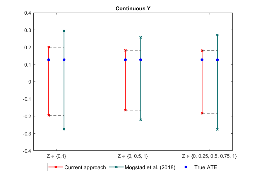
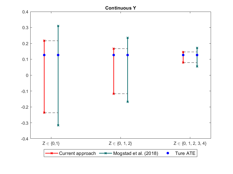
Figure 9: Full vs. Mean Independence: Bounds on ATE with Continuous $Y$

Next, the manner in which the bounds are affected by the cardinality of $\mathcal{Z}$ is unclear in Section 8.2. This is because we fix the endpoints of $Z$. Intuitively, if the endpoints of $\mathcal{Z}$ move further away, the bound would shrink. Figure 10 shows that this is in fact the case.

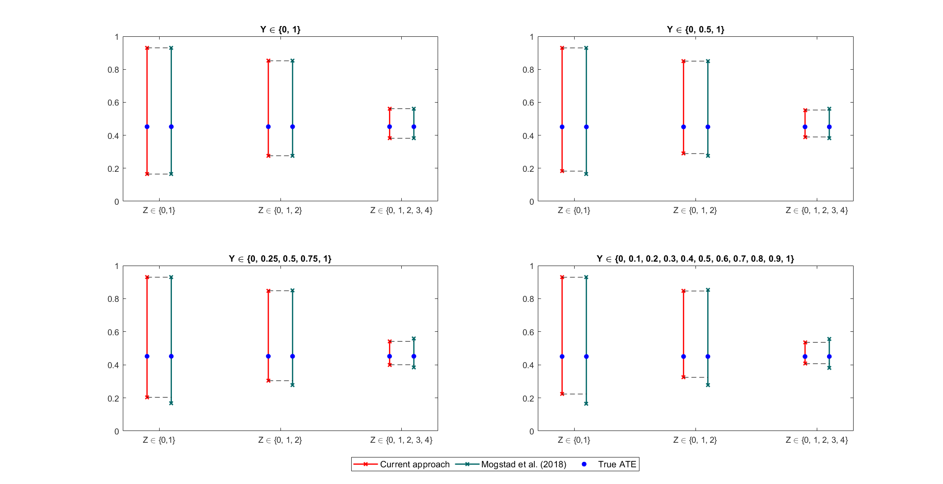
Figure 10: Bounds on ATE for Different Support of $\mathcal{Z}$

D.2 Common Exogenous Variable

In Section 8, we set $W$ to be a reverse IV in our main DGP. It is important to note that what matters for identifying power is the exogeneity of $W$ and not the reverse exclusion of $W$. To clarify this point, we compare the results derived from a reverse IV with those from a common exogenous variable. For the latter, we use the main DGP in Section 8.

Figure 11 exhibits very similar results between the reverse IV and the common exogenous variable. This evidence suggests that the crucial role in improving the bounds lies in the exogeneity of $W$, rather than its reverse exclusion.

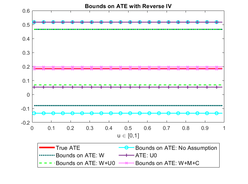
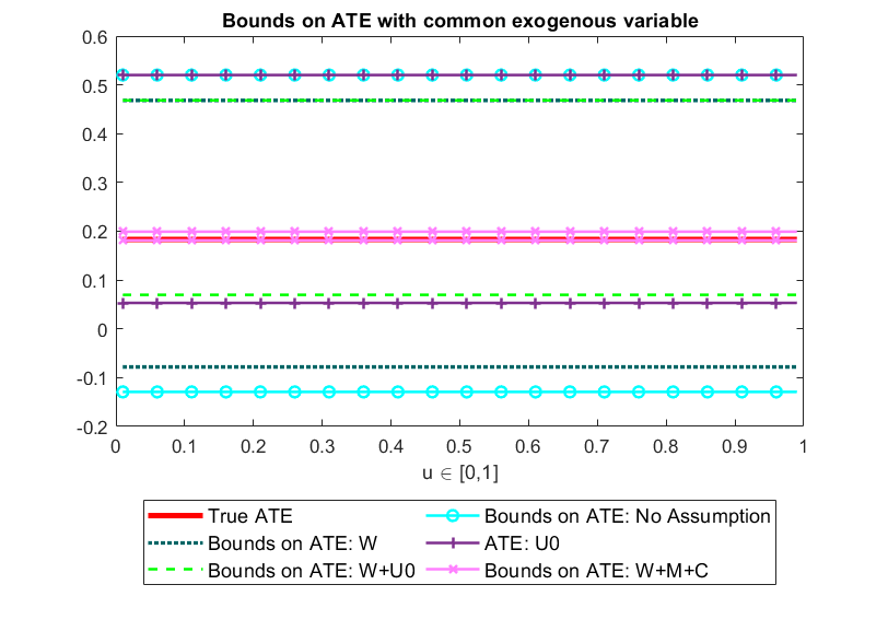
Figure 11: Comparison with Common Exogenous Variable vs. Reverse IV

D.3 Discussions on Misspecification

For sieve approximations, implicit smoothness assumptions are inherent. It would be crucial to evaluate the extent of misspecification using a DGP that exhibits the lack of smoothness. To demonstrate the possibility of misspecification within our approach and further illustrate the choice of $K$, we select a DGP where the MTE function is defined as $m_{1}(u)-m_{0}(u)=0.7\cdot|sin(2\pi u)|$. Note that the sine function is difficult to approximate in general. Moreover, the MTE has kink points, which the Bernstein approximation would fail to capture. Under this DGP, the pointwise bound for the MTE function with varying polynomial orders $K$ is depicted in Figure 12. When $K$ is set as low as 5, the sieve approximation incurs severe misspecification in that the bound only covers the true MTE over a brief interval among the compliers. From $K=10$ onwards, the bounds cover most of the true MTE except the middle part. While all polynomials orders fail to capture the kink point, the magnitude of misspecification diminishes when $K$ is large.

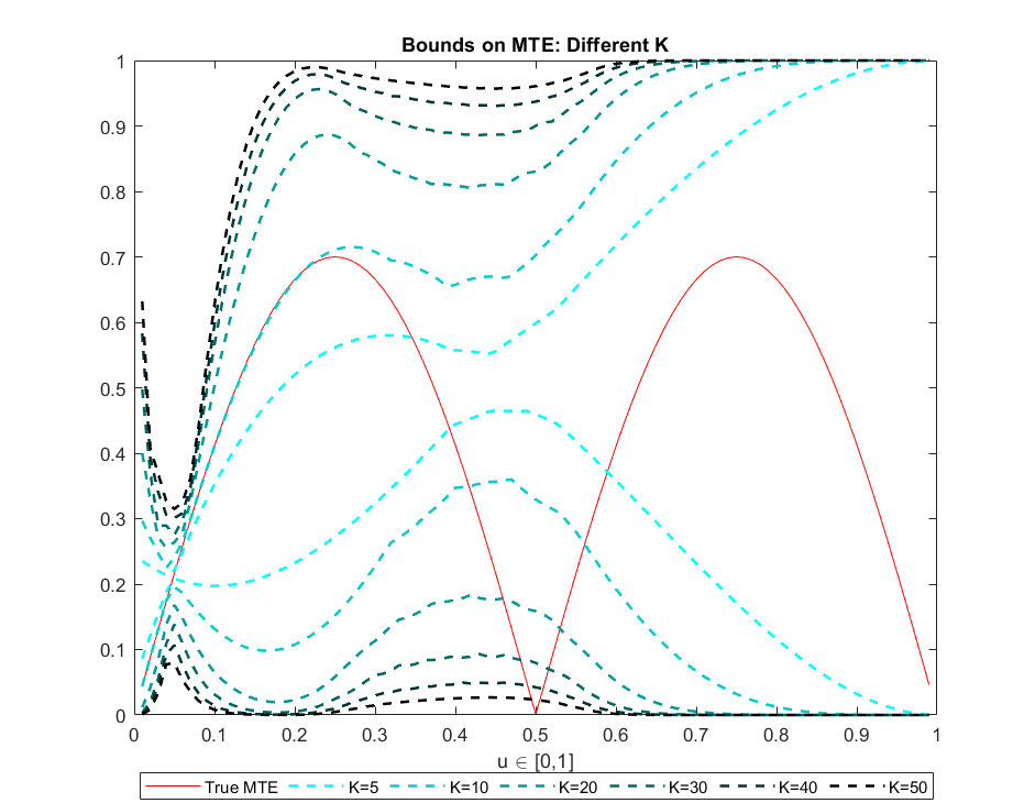
Figure 12: Bounds on Non-Smooth MTE with Different $K$

To more clearly compare the magnitude of misspecification across the choices of $K$, we select 100 evenly-spaced points on $\mathcal{U}=[0,1]$, and compute the Hausdorff distance for the set of $u$ where the MTE falls outside the identified set. Figure 13 show a significant reduction in the magnitude of misspecification when $K$ takes larger values.

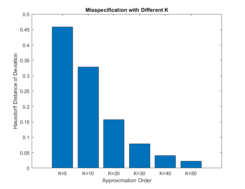
Figure 13: Misspecification with Different $K$

References

- Angrist and Fernandez-Val (2010) Angrist, J. and I. Fernandez-Val (2010): “Extrapolate-ing: External validity and overidentification in the late framework,” Tech. rep., National Bureau of Economic Research.
- Balat and Han (2020) Balat, J. and S. Han (2020): “Multiple treatments with strategic substitutes,” Forthcoming in Journal of Econometrics.
- Balke and Pearl (1997) Balke, A. and J. Pearl (1997): “Bounds on treatment effects from studies with imperfect compliance,” Journal of the American Statistical Association, 92, 1171–1176.
- Beresteanu et al. (2011) Beresteanu, A., I. Molchanov, and F. Molinari (2011): “Sharp identification regions in models with convex moment predictions,” Econometrica, 79, 1785–1821.
- Bertanha and Imbens (2019) Bertanha, M. and G. W. Imbens (2019): “External validity in fuzzy regression discontinuity designs,” Journal of Business & Economic Statistics, 1–39.
- Bhattacharya et al. (2008) Bhattacharya, J., A. M. Shaikh, and E. Vytlacil (2008): “Treatment effect bounds under monotonicity assumptions: an application to Swan-Ganz catheterization,” American Economic Review, 98, 351–56.
- Brinch et al. (2017) Brinch, C. N., M. Mogstad, and M. Wiswall (2017): “Beyond LATE with a discrete instrument,” Journal of Political Economy, 125, 985–1039.
- Carnicer and Pena (1993) Carnicer, J. M. and J. M. Pena (1993): “Shape preserving representations and optimality of the Bernstein basis,” Advances in Computational Mathematics, 1, 173–196.
- Chen (2007) Chen, X. (2007): “Large sample sieve estimation of semi-nonparametric models,” Handbook of econometrics, 6, 5549–5632.
- Chen and Christensen (2018) Chen, X. and T. M. Christensen (2018): “Optimal sup-norm rates and uniform inference on nonlinear functionals of nonparametric IV regression,” Quantitative Economics, 9, 39–84.
- Chen et al. (2011) Chen, X., E. T. Tamer, and A. Torgovitsky (2011): “Sensitivity analysis in semiparametric likelihood models,” .
- Chen et al. (2017) Chen, X., J. Tan, Z. Liu, and J. Xie (2017): “Approximation of functions by a new family of generalized Bernstein operators,” Journal of Mathematical Analysis and Applications, 450, 244–261.
- Chernozhukov and Hansen (2005) Chernozhukov, V. and C. Hansen (2005): “An IV model of quantile treatment effects,” Econometrica, 73, 245–261.
- Chernozhukov et al. (2013) Chernozhukov, V., S. Lee, and A. M. Rosen (2013): “Intersection bounds: estimation and inference,” Econometrica, 81, 667–737.
- Chiburis (2010a) Chiburis, R. C. (2010a): “Semiparametric bounds on treatment effects,” Journal of Econometrics, 159, 267–275.
- Chiburis (2010b) ——— (2010b): “Semiparametric bounds on treatment effects,” Journal of Econometrics, 159, 267–275.
- Coolidge (1949) Coolidge, J. L. (1949): “The story of the binomial theorem,” The American Mathematical Monthly, 56, 147–157.
- Cornelissen et al. (2016) Cornelissen, T., C. Dustmann, A. Raute, and U. Schönberg (2016): “From LATE to MTE: Alternative methods for the evaluation of policy interventions,” Labour Economics, 41, 47–60.
- Deb et al. (2023) Deb, R., Y. Kitamura, J. K. Quah, and J. Stoye (2023): “Revealed price preference: theory and empirical analysis,” The Review of Economic Studies, 90, 707–743.
- Dehejia et al. (2019) Dehejia, R., C. Pop-Eleches, and C. Samii (2019): “From local to global: External validity in a fertility natural experiment,” Journal of Business & Economic Statistics, 1–27.
- Dunlop et al. (2002) Dunlop, D. D., L. M. Manheim, J. Song, and R. W. Chang (2002): “Gender and ethnic/racial disparities in health care utilization among older adults,” The Journals of Gerontology Series B: Psychological sciences and social sciences, 57, S221–S233.
- Eisenhauer et al. (2015) Eisenhauer, P., J. J. Heckman, and E. Vytlacil (2015): “The generalized Roy model and the cost-benefit analysis of social programs,” Journal of Political Economy, 123, 413–443.
- Fang et al. (2020) Fang, Z., A. Santos, A. Shaikh, and A. Torgovitsky (2020): “Inference for large-scale linear systems with known coefficients,” University of Chicago, Becker Friedman Institute for Economics Working Paper.
- Finkelstein et al. (2012) Finkelstein, A., S. Taubman, B. Wright, M. Bernstein, J. Gruber, J. P. Newhouse, H. Allen, K. Baicker, and O. H. S. Group (2012): “The Oregon health insurance experiment: evidence from the first year,” The Quarterly journal of economics, 127, 1057–1106.
- Firpo and Ridder (2019) Firpo, S. and G. Ridder (2019): “Partial identification of the treatment effect distribution and its functionals,” Journal of Econometrics, 213, 210–234.
- Freyberger and Horowitz (2015) Freyberger, J. and J. L. Horowitz (2015): “Identification and shape restrictions in nonparametric instrumental variables estimation,” Journal of Econometrics, 189, 41–53.
- Goodman (1989) Goodman, T. (1989): “Shape preserving representations,” in Mathematical methods in computer aided geometric design, Elsevier, 333–351.
- Goodman et al. (1999) Goodman, T. N., H. Oruç, and G. M. Phillips (1999): “Convexity and generalized Bernstein polynomials,” Proceedings of the Edinburgh Mathematical Society, 42, 179–190.
- Gu and Russell (2022) Gu, J. and T. M. Russell (2022): “Partial identification in nonseparable binary response models with endogenous regressors,” Journal of Econometrics.
- Gunsilius (2019) Gunsilius, F. (2019): “Bounds in continuous instrumental variable models,” arXiv preprint arXiv:1910.09502.
- Hafsa and Mandallena (2003) Hafsa, O. A. and J.-P. Mandallena (2003): “Interchange of infimum and integral,” Calculus of Variations and Partial Differential Equations, 18, 433–449.
- Han (2019) Han, S. (2019): “Optimal dynamic treatment regimes and partial welfare ordering,” arXiv preprint arXiv:1912.10014.
- Han (2020) ——— (2020): “Nonparametric estimation of triangular simultaneous equations models under weak identification,” Quantitative Economics, 11, 161–202.
- Han (2021) ——— (2021): “Identification in nonparametric models for dynamic treatment effects,” Journal of Econometrics, 225, 132–147.
- Han and Lee (2019) Han, S. and S. Lee (2019): “Estimation in a generalization of bivariate probit models with dummy endogenous regressors,” Journal of Applied Econometrics, 34, 994–1015.
- Han and Vytlacil (2017) Han, S. and E. J. Vytlacil (2017): “Identification in a generalization of bivariate probit models with dummy endogenous regressors,” Journal of Econometrics, 199, 63–73.
- Han and Xu (2023) Han, S. and H. Xu (2023): “On Quantile Treatment Effects, Rank Similarity, and Multiple Instrumental Variables,” .
- Heckman (2010) Heckman, J. J. (2010): “Building bridges between structural and program evaluation approaches to evaluating policy,” Journal of Economic literature, 48, 356–98.
- Heckman and Vytlacil (2005) Heckman, J. J. and E. Vytlacil (2005): “Structural equations, treatment effects, and econometric policy evaluation1,” Econometrica, 73, 669–738.
- Heckman and Vytlacil (1999) Heckman, J. J. and E. J. Vytlacil (1999): “Local instrumental variables and latent variable models for identifying and bounding treatment effects,” Proceedings of the national Academy of Sciences, 96, 4730–4734.
- Heckman and Vytlacil (2001) ——— (2001): Instrumental variables, selection models, and tight bounds on the average treatment effect, Springer.
- Honoré and Lleras-Muney (2006) Honoré, B. E. and A. Lleras-Muney (2006): “Bounds in competing risks models and the war on cancer,” Econometrica, 74, 1675–1698.
- Honoré and Tamer (2006) Honoré, B. E. and E. Tamer (2006): “Bounds on parameters in panel dynamic discrete choice models,” Econometrica, 74, 611–629.
- Hsieh et al. (2022) Hsieh, Y.-W., X. Shi, and M. Shum (2022): “Inference on estimators defined by mathematical programming,” Journal of Econometrics, 226, 248–268.
- Hurd and McGarry (1997) Hurd, M. D. and K. McGarry (1997): “Medical insurance and the use of health care services by the elderly,” Journal of Health Economics, 16, 129–154.
- Imbens and Angrist (1994) Imbens, G. W. and J. D. Angrist (1994): “Identification and Estimation of Local Average Treatment Effects,” Econometrica, 62, 467–475.
- Joy (2000) Joy, K. I. (2000): “Bernstein polynomials,” On-Line Geometric Modeling Notes, 13.
- Kamat (2019) Kamat, V. (2019): “Identification with latent choice sets: The case of the head start impact study,” arXiv preprint arXiv:1711.02048.
- Kowalski (2021) Kowalski, A. E. (2021): “Reconciling seemingly contradictory results from the Oregon health insurance experiment and the Massachusetts health reform,” The Review of Economics and Statistics, 1–45.
- Liu et al. (2020) Liu, S., I. Mourifié, and Y. Wan (2020): “Two-way exclusion restrictions in models with heterogeneous treatment effects,” The Econometrics Journal, 23, 345–362.
- Machado et al. (2019) Machado, C., A. Shaikh, and E. Vytlacil (2019): “Instrumental variables and the sign of the average treatment effect,” Journal of Econometrics, 212, 522–555.
- Manski (1990) Manski, C. F. (1990): “Nonparametric bounds on treatment effects,” The American Economic Review, 80, 319–323.
- Manski (1997) ——— (1997): “Monotone treatment response,” Econometrica: Journal of the Econometric Society, 1311–1334.
- Manski and Pepper (2000) Manski, C. F. and J. V. Pepper (2000): “Monotone instrumental variables: With an application to the returns to schooling,” Econometrica, 68, 997–1010.
- Marx (2020) Marx, P. (2020): “Sharp Bounds in the Latent Index Selection Model,” arXiv preprint arXiv:2012.02390.
- Masten and Poirier (2021) Masten, M. A. and A. Poirier (2021): “Salvaging falsified instrumental variable models,” Econometrica, 89, 1449–1469.
- Mogstad et al. (2017) Mogstad, M., A. Santos, and A. Torgovitsky (2017): “Using Instrumental Variables for Inference about Policy Relevant Treatment Effects,” Tech. rep., National Bureau of Economic Research.
- Mogstad et al. (2018) ——— (2018): “Using instrumental variables for inference about policy relevant treatment parameters,” Econometrica, 86, 1589–1619.
- Mogstad et al. (2021) Mogstad, M., A. Torgovitsky, and C. R. Walters (2021): “The causal interpretation of two-stage least squares with multiple instrumental variables,” American Economic Review, 111, 3663–98.
- Mourifié (2015) Mourifié, I. (2015): “Sharp bounds on treatment effects in a binary triangular system,” Journal of Econometrics, 187, 74–81.
- Muralidharan et al. (2019) Muralidharan, K., A. Singh, and A. J. Ganimian (2019): “Disrupting education? Experimental evidence on technology-aided instruction in India,” American Economic Review, 109, 1426–60.
- Russell (2021) Russell, T. M. (2021): “Sharp bounds on functionals of the joint distribution in the analysis of treatment effects,” Journal of Business & Economic Statistics, 39, 532–546.
- Shaikh and Vytlacil (2011) Shaikh, A. M. and E. J. Vytlacil (2011): “Partial identification in triangular systems of equations with binary dependent variables,” Econometrica, 79, 949–955.
- Simon (1986) Simon, J. (1986): “Compact sets in the space L p (O, T; B),” Annali di Matematica pura ed applicata, 146, 65–96.
- Taubman et al. (2014) Taubman, S. L., H. L. Allen, B. J. Wright, K. Baicker, and A. N. Finkelstein (2014): “Medicaid increases emergency-department use: evidence from Oregon’s Health Insurance Experiment,” Science, 343, 263–268.
- Torgovitsky (2019a) Torgovitsky, A. (2019a): “Nonparametric inference on state dependence in unemployment,” Econometrica, 87, 1475–1505.
- Torgovitsky (2019b) ——— (2019b): “Partial identification by extending subdistributions,” Quantitative Economics, 10, 105–144.
- Vuong and Xu (2017) Vuong, Q. and H. Xu (2017): “Counterfactual mapping and individual treatment effects in nonseparable models with binary endogeneity,” Quantitative Economics, 8, 589–610.
- Vytlacil (2002) Vytlacil, E. (2002): “Independence, monotonicity, and latent index models: An equivalence result,” Econometrica, 70, 331–341.
- Vytlacil and Yildiz (2007) Vytlacil, E. and N. Yildiz (2007): “Dummy endogenous variables in weakly separable models,” Econometrica, 75, 757–779.