Equilibrium orientation and adsorption of an ellipsoidal Janus particle at a fluid-fluid interface

Abstract

We investigate the equilibrium orientation and adsorption process of a single, ellipsoidal Janus particle at a fluid-fluid interface. The particle surface comprises equally sized parts that are hydrophobic or hydrophilic. We present free energy models to predict the equilibrium orientation and compare the theoretical predictions with lattice Boltzmann simulations. We find that the deformation of the fluid interface strongly influences the equilibrium orientation of the Janus ellipsoid. The adsorption process of the Janus ellipsoid can lead to different final orientations determined by the interplay of particle aspect ratio and particle wettablity contrast.

I Introduction

Janus particles have drawn great attention recently for their potential in various applications, such as micro-swimmers, stabilizers of emulsions and catalysis Walther2013a ; FernandezRodriguez2014a ; FernandezRodriguez2016a ; Archer2018 ; Marschelke2020 . The special characteristics of these particles include their anisotropic physical (e.g. optical, electric, or magnetic) or chemical (e.g. wetting or catalytic) properties at well-defined areas on their surface. Amphiphilic Janus particles are characterized by opposite wetting abilities at their hemispheres and have been shown to attach strongly at fluid-fluid interfaces Morris2015a ; Park2012a ; Park2012b ; Hirose2007a ; Binks2001b . Binks et al. Binks2001b compared the free energy of homogeneous spherical particles and Janus spherical particles in contact with a fluid interface. They found that the free energy of amphiphilic Janus particles can be $3$ times larger than that of homogeneous particles. Furthermore, Janus particles retain strong adsorption at interfaces even for contact angles of $0^{\circ}$ and $180^{\circ}$. Thus, Janus particles are generally expected to be more efficient emulsion stabilizers than homogeneous colloidal particles Fan2012 ; Mejia2012 ; Hirose2007a .

The understanding of the equilibrium orientation and the adsorption dynamics of Janus particles at fluid interfaces is critical to enable their optimal utilization. Park et al. theoretically studied the configurations of Janus ellipsoids at a fluid interface Park2012a ; Park2012b , and found that the orientation of ellipsoidal Janus particles is affected by the particle aspect ratio and the Janus character given by the wettability contrast. In their model, they used a flat-interface approach, where the dynamic deformation of interface during the adsorption process is neglected. However, numerical studies of ellipsoidal Janus particles at fluid interfaces demonstrated that the interface deforms around the particle and thus, the interface deformation is expected to affect the equilibrium orientation of particles Rezvantalab2013a ; Hirose2007a ; Anzivino2019 ; XieHarting2020 .

Here, we present a simplified free energy model of an ellipsoidal Janus particle at a non-deforming fluid-fluid interface and then extend it by taking into account the interface deformation. The theoretical models are used to predict the equilibrium orientation of the particle, and are compared to our numerical results obtained from lattice Boltzmann simulations. Moreover, we numerically study the adsorption process of a Janus ellipsoid with varying the particle aspect ratio and the Janus character, i.e. the wettability contrast.

The remainder of this paper is organized as follows. In Sec. II we introduce our simulation method and setup, followed by a comparison of the simplified free energy model with simulations in Sec. III. Sec. IV extends towards deformable interfaces. In Sec. V we demonstrate how the adsorption trajectories of an ellipsoidal Janus particle depend on the interplay between particle aspect ratio and wettability contrast. Finally, we conclude the paper with a short summary.

II Simulation method

Here, we summarize the main ingredients of our simulation method. A more detailed description can be found in our previous publications on particle-laden multicomponent flows Frijters2012a ; Guenther2012a ; Krueger2012c ; Guenther2013a ; Guenther2013b ; Guenther2014a . We use the lattice Boltzmann (LB) method succi2001a to simulate two immiscible fluids $c$, $c^{\prime}$ where the discrete form of the Boltzmann equation can be written as

$$f_{i}^{c}(\mathbf{x}+\vec{c}_{i}\Delta t,t+\Delta t)=f_{i}^{c}(\mathbf{x},t)+\Omega_{i}^{c}(\mathbf{x},t)\mbox{.}$$ (1)

Here, $f_{i}^{c}(\mathbf{x},t)$ is the single-particle distribution function for fluid component $c$ with discrete lattice velocity $\vec{c}_{i}$ at time $t$ located at lattice position $\mathbf{x}$. We use a D3Q19 lattice, i.e. a 3D lattice with a lattice constant $\Delta x$ and nineteen velocity directions. $\Delta t$ is the timestep and

$$\Omega_{i}^{c}(\mathbf{x},t)=-\frac{f_{i}^{c}(\mathbf{x},t)-f_{i}^{\mathrm{eq}}(\rho^{c}(\mathbf{x},t),\vec{u}^{c}(\mathbf{x},t))}{\left(\tau^{c}/\Delta t\right)}$$ (2)

is the Bhatnagar-Gross-Krook (BGK) collision operator bhatnagar1954a . The density is defined as $\rho^{c}(\mathbf{x},t)=\rho_{0}\sum_{i}f_{i}^{c}(\mathbf{x},t)$, where $\rho_{0}$ is a reference density. $\tau^{c}$ is the relaxation time for the component $c$ and $f_{i}^{\mathrm{eq}}(\rho^{c},\vec{u}^{c})$ is the equilibrium distribution function. $\vec{u}^{c}(\mathbf{x},t)=\sum_{i}f_{i}^{c}(\mathbf{x},t)\vec{c}_{i}/\rho^{c}(\mathbf{x},t)$ is the local velocity. The kinematic viscosity can be calculated as

$$\nu^{c}=c_{s}^{2}\Delta t\left(\frac{\tau^{c}}{\Delta t}-\frac{1}{2}\right)\mbox{,}$$ (3)

where $c_{s}=\frac{1}{\sqrt{3}}\frac{\Delta x}{\Delta t}$ is the speed of sound. In the following, we choose $\Delta x=\Delta t=\rho_{0}=1$ for simplicity. Furthermore, in all simulations, the relaxation time is set to $\tau^{c}\equiv 1$.

We use the method introduced by Shan and Chen for the simulation of a multicomponent fluid mixture shan1993a . Every species has its own distribution function following Eq. (1) and an interaction between the different components is introduced as

$$\vec{F}^{c}(\mathbf{x},t)=-\Psi^{c}(\mathbf{x},t)\sum_{c^{\prime}}g_{cc^{\prime}}\sum_{\mathbf{x}^{\prime}}\Psi^{c^{\prime}}(\mathbf{x}^{\prime},t)(\mathbf{x}^{\prime}-\mathbf{x})\mbox{.}$$ (4)

The resulting force is included in the equilibrium distribution function (Eq. (2)) by shifting the velocity $\vec{u}^{c}(\mathbf{x},t)$. $g_{cc^{\prime}}$ is the interaction parameter between the fluid components $c$ and $c^{\prime}$ and defines the surface tension and $\Psi^{c}(\mathbf{x},t)=\rho_{0}[1-\exp({-\rho^{c}(\mathbf{x},t)/\rho_{0}})]$ is a functional defining the equation of state of the system.

The particles follow Newton’s equations of motion and are discretized on the lattice. They are coupled to both fluid species by a modified bounce-back boundary condition which was originally introduced by Ladd Jansen2011a ; aidun1998a ; ladd1994a ; ladd1994b ; ladd2001a ; KHH04 . If the particle moves, some lattice nodes become free and others become occupied. The momentum of the fluid on the newly occupied nodes is transferred to the particle. A newly freed node (located at $\mathbf{x}$) is filled with the average density of the $N_{\mathrm{FN}}$ neighboring fluid lattice nodes $\mathbf{x}_{i_{\mathrm{FN}}}$ for each component $c$,

$$\overline{\rho}^{c}(\mathbf{x},t)\equiv\frac{1}{N_{\mathrm{FN}}}\sum_{i_{\mathrm{FN}}}\rho^{c}(\mathbf{x}+\vec{c}_{i_{\mathrm{FN}}},t)\mbox{.}$$ (5)

The fluid interaction forces also act between a node in the outer shell of a particle and its neighboring point outside of the particle. Since this would lead to an increase of the fluid density around the particle, the nodes in the outer shell of the particle are filled with a virtual fluid corresponding to the average of the value in the neighboring free nodes for each fluid component: $\rho_{\mathrm{virt}}^{c}(\mathbf{x},t)=\overline{\rho}^{c}(\mathbf{x},t)$. This can be used to control the wettability properties of the particle surface for the special case of two fluid species which will be named red and blue. We define the parameter $\Delta\rho$ and call it particle color. For positive values of $\Delta\rho$ we add it to the fluid component $c$, $\rho_{\mathrm{virt}}^{c}=\overline{\rho}^{c}+\Delta\rho$, while for negative values we add its absolute value to another fluid component $c^{\prime}$, $\rho_{\mathrm{virt}}^{c^{\prime}}=\overline{\rho}^{c^{\prime}}+|\Delta\rho|$.

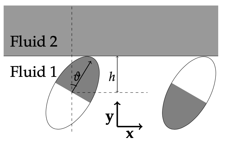
Figure 1: A single ellipsoidal Janus particle touching a fluid-fluid interface: $h$ is the distance between the particle center and the flat fluid interface, $\vartheta$ is the particle orientation. Fluid 1 is defined as the fluid in which the particle is immersed in the beginning and fluid 2 is the fluid into which the particle enters. The dark area of the Janus particle prefers fluid 2 whereas the white area prefers fluid 1. The left particle is in the “preferred initial orientation” (PIO, $0\leq\vartheta_{0}<90^{\circ}$) and the right particle in the “unpreferred initial orientation” (UIO, $90^{\circ}<\vartheta_{0}\leq 180^{\circ}$).

Our simulation setup is illustrated in Fig. 1 and consists of a cubic volume composed of two equally sized layers of two immiscible fluids such as oil and water with density 0.7 each. With setting the coupling constant $g_{cc^{\prime}}=0.1$, we obtain a surface tension of $\sigma_{12}\approx 0.041$ and our fluids form a flat fluid-fluid interface. The system is confined by walls at the top and the bottom. Periodic boundary conditions apply in the $x$- and $z$-direction parallel to the interface.

We restrict ourselves to symmetric ellipsoidal Janus particles with an aspect ratio $m$. $R_{\parallel}$ and $R_{\perp}$ are the parallel and orthogonal radius of the ellipsoid, respectively (The parallel radius is chosen as $R_{\parallel}=8$ if not defined otherwise.). The particle surface is divided into two equal proportions: a more apolar region with a contact angle $\theta_{A}=90^{\circ}+\Delta\theta$ and a more polar region with a contact angle $\theta_{P}=90^{\circ}-\Delta\theta$. The Janus influence is given by the parameter $\Delta\theta$. Both areas of different wettability have exactly the same size. The position and the orientation of the particle with respect to the undeformed, flat interface are characterized by the variables $\xi$ and $\vartheta$, respectively. $\xi$ is the distance between the undeformed interface and the particle center in units of $R_{\parallel}$, $\xi=h/R_{\parallel}$ and $\vartheta$ is the polar angle and given as the angle between the main axis and the interface normal. The particle is initially placed so that it just touches the flat interface with different initial orientations $\vartheta_{0}=\vartheta(t=0)$ and initial positions $\xi_{0}=\xi(t=0)$.

The particle can be placed in two different ways as shown in Fig. 1. It adsorbs to the interface between the fluids 1 and 2. Here, fluid 1 is defined as the fluid where the particle is immersed at the start of the simulation and fluid 2 is the fluid in which the particle enters during the adsorption process. The Janus particle is divided into an area which prefers fluid 1 (white area in Fig. 1) and one preferring fluid 2 (dark area in Fig. 1). This leads to two possible situations of the initial particle orientation for the adsorbing process: the first orientation range is the “preferred initial orientation” (PIO) with $0\leq\vartheta_{0}<90^{\circ}$ (left particle in Fig. 1), where the wetting area preferring fluid 2 touches the interface and enters fluid 2. The next one is the “unpreferred initial orientation” (UIO) with $90^{\circ}<\vartheta_{0}\leq 180^{\circ}$ (right particle in Fig. 1), where the oppositely wetting area is at the interface. In case of $\vartheta_{0}=90^{\circ}$, the border between both wetting areas touches the interface. $\vartheta^{\prime}$ is defined as the effective polar angle and given as

$$\vartheta^{\prime}=\begin{cases}\vartheta,&\text{for }\vartheta\leq 90^{\circ}\\ 180^{\circ}-\vartheta,&\text{for }\vartheta>90^{\circ}\mbox{.}\end{cases}$$ (6)

Five reference values for the effective initial orientation $\vartheta_{0}^{\prime}$ are chosen as

$$\vartheta_{0}^{\prime}=n_{\vartheta}22.5^{\circ}\text{, }n_{\vartheta}=\{0,1,2,3,4\}\mbox{.}$$ (7)

All these initial orientations $\vartheta_{0}^{\prime}$ are taken for the PIO and the UIO. $\vartheta_{0}^{\prime}=(10^{-4})^{\circ}$ is chosen as an additional orientation and only useful for the PIO as a hint if the upright orientation ($\vartheta=0$) is a minimum of the free energy.

III A simplified free energy model for Janus particles

In this section we present a simplified free energy model for a single Janus particle at a flat fluid interface. The following two assumptions are made: first, we consider an undeformable, flat interface. Second, only the extreme particle orientations parallel and orthogonal to the interface are taken into account. The upright orientation is the one where each wetting area is fully immersed in its preferred fluid. This orientation is expected if the Janus effect dominates. The parallel orientation is the orientation, where the particle occupies as much interfacial area as possible. This orientation is expected if the shape of the particle dominates. This model is referred to in the following as the “simplified Janus model”.

The free energy of the system is given as

$${\cal F}(\xi,\vartheta)=\sigma_{12}A_{12}+\sum_{i=1,2}\sum_{j=A,P}\sigma_{ij}A_{ij}\mbox{.}$$ (8)

$A$ and $\sigma$ are the interface areas and the interfacial tensions, respectively. 1 and 2 denote the two fluids whereas $P$ and $A$ denote the polar and apolar region of the particle surface, respectively.

We consider the initial state where the particle is fully immersed in fluid 1 which changes Eq. (8) to

$${\cal F}_{0}=\sigma_{12}A_{\rm flat}+\frac{1}{2}A_{\rm ell}(\sigma_{1A}+\sigma_{1P})\mbox{.}$$ (9)

$A_{\rm ell}$ is the total area of the ellipsoid surface. $A_{\rm flat}$ is the area of the flat fluid interface in absence of the particle. ${\cal F}_{0}$ is the free energy of the reference state where the particle is immersed in the bulk and away from the interface. For the final particle orientation parallel to the interface ($\vartheta_{\rm final}=90^{\circ}$), Eq. (8) changes to

$${\cal F}_{\parallel}=(A_{\rm flat}-A_{\parallel})\sigma_{12}+0.25A_{\rm ell}\left(\sum_{i=1,2}(\sigma_{iP}+\sigma_{iA})\right)\mbox{.}$$ (10)

$A_{\rm flat}-A_{\parallel}$ is the remaining fluid-fluid interface after the particle adsorption and $A_{\parallel}$ is the area of the fluid-fluid interface excluded by the particle oriented parallel to the interface. The free energy difference is given as $\Delta{\cal F}_{\parallel}={\cal F}_{\parallel}-{\cal F}_{0}=-A_{\parallel}\sigma_{12}+0.25A_{\rm ell}(\sum_{i=A,P}(\sigma_{2i}-\sigma_{1i}))$. Using Young’s equation $\sigma_{12}\cos\theta=\sigma_{2p}-\sigma_{1p}$ which holds for both of the two wetting areas of the particle independently, we obtain

$$\Delta{\cal F}_{\parallel}=\sigma_{12}\left(0.25A_{\rm ell}\left(\sum_{i=A,P}\cos\theta_{i}\right)-A_{\parallel}\right)\mbox{.}$$ (11)

Furthermore, assuming $\cos\theta_{A}=-\cos\theta_{P}$ to simplify Eq. (11), we get

$$\Delta{\cal F}_{\parallel}=-\sigma_{12}A_{\parallel}\mbox{.}$$ (12)

For the particle orientation parallel to the interface normal, the free energy is given as ${\cal F}_{\perp}=(A_{\rm flat}-A_{\perp})\sigma_{12}+0.5A_{\rm ell}(\sigma_{1A}+\sigma_{2P})$. $A_{\perp}$ is the excluded interfacial area due to a particle with orthogonal orientation. In the same way as above, we get $\Delta{\cal F}_{\perp}={\cal F}_{\perp}-{\cal F}_{0}=-A_{\perp}\sigma_{12}+0.5A_{\rm ell}(\sigma_{2P}-\sigma_{1P})$ and reach the following relation:

$$\Delta{\cal F}_{\perp}=-\sigma_{12}(0.5A_{\rm ell}\cos\theta_{P}+A_{\perp})=-\sigma_{12}(0.5A_{\rm ell}\sin\Delta\theta+A_{\perp})\mbox{,}$$ (13)

with $\cos\theta_{P}=\sin\Delta\theta$. In order to find the orientation of the stable point of the Janus particle at the interface, it is necessary to find the global minimum of the free energy. $\Delta\theta_{t}$ is defined as the transition value of $\Delta\theta$ above which the particle orientation parallel to the interface normal minimizes the free energy. Comparing Eq. (12) and Eq. (13) leads to the following value of $\Delta\theta_{t}$ for the transition point:

$$\sin\Delta\theta_{t}=\frac{2(A_{\parallel}-A_{\perp})}{A_{\rm ell}}\mbox{.}$$ (14)

Thus, $\sin\Delta\theta_{t}$ depends on the aspect ratio via the three interfacial areas, which are given as

$$\begin{split}0.5A_{\rm ell}&=\pi R_{\perp}^{2}+\frac{\pi R_{\perp}R_{\parallel}^{2}}{\sqrt{R_{\parallel}^{2}-R_{\perp}^{2}}}\arcsin\left(\frac{\sqrt{R_{\parallel}^{2}-R_{\perp}^{2}}}{R_{\parallel}}\right),\\ &=\pi R_{\perp}^{2}\left(1+\frac{m}{\sqrt{m^{2}-1}}\arcsin\left(\frac{\sqrt{m^{2}-1}}{m}\right)\right)\mbox{,}\\ A_{\perp}&=\pi R_{\perp}^{2},\\ A_{\parallel}&=\pi R_{\perp}R_{\parallel}=\pi mR_{\perp}^{2}\mbox{.}\end{split}$$ (15)

This changes Eq. (14) to the following relation for $\Delta\theta_{t}(m)$:

$$\sin\Delta\theta_{t}=\frac{m-1}{\left(1+\frac{m}{\sqrt{m^{2}-1}}\arcsin\left(\frac{\sqrt{m^{2}-1}}{m}\right)\right)}\mbox{.}$$ (16)

This result relates the Janus parameter at the transition point to the aspect ratio of the particle. As an example, for $m=2$, we obtain $\Delta\theta_{t}\approx 17^{\circ}$. The function given in Eq. (16) is shown in Fig. 2 for the range of the aspect ratio which is used in the simulation of the particle adsorption below ($1\leq m\leq 6$). The parallel orientation minimizes the free energy below the line and the upright orientation above.

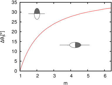
Figure 2: The phase diagram ($\Delta\theta_{t}$-$m$) obtained from the “simplified Janus model”. In the area above the line the upright orientation is the stable state whereas ibelow the line the particle orientation parallel to the interface is the stable state. The line represents Eq. (16).

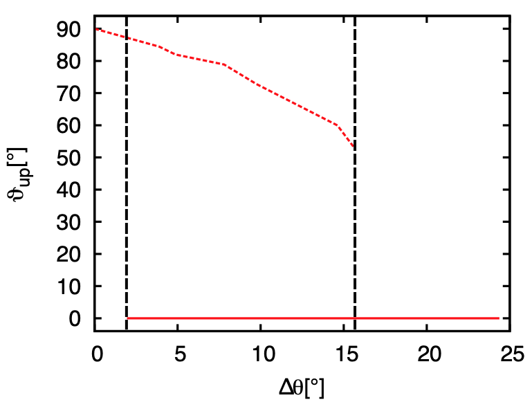
Figure 3: Final orientation of a Janus particle for $m=1.5$. A tilted (red dashed line) and an upright (red solid line) orientation of the particle are shown depending on the Janus parameter $\Delta\theta$. The vertical dashed lines divide the range of $\Delta\theta$ into three regions. In the left region, it can be concluded from the simulation results that the tilted orientation is the global minimum. In the right region, the upright orientation is the only one which is found. In the central region, both tilted and upright orientations are found in the simulation results. It cannot be seen which one corresponds to the energetic minimum.

In the following, we compare the predictions from the simplified model to our simulations. We follow several paths through the $m$-$\Delta\theta$ phase diagram from Fig. 2 and compare the equilibrium orientation with the final particle orientations obtained from the simulation. At first, we follow the lines along a constant aspect ratio $m$ with a varying Janus parameter $\Delta\theta$. This corresponds to a vertical line through the phase diagram.

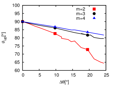
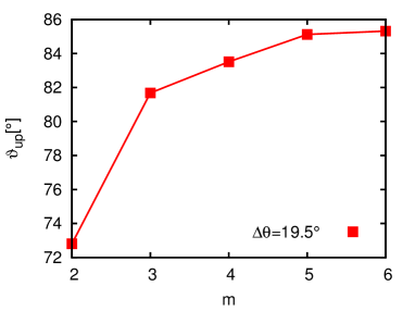
Figure 4: (a) The final value of the angle $\vartheta_{\rm up}$ after the adsorption of the particle to the fluid interface in the tilted state is shown for a constant aspect ratio $m$ and as a function of the Janus parameter $\Delta\theta$. (b) The final angle $\vartheta_{\rm up}$ of the particle after the adsorption to a fluid interface in the tilted state is shown for a constant $\Delta\theta$ and depending on $m$.

It is shown for $m=1.5$ in Fig. 3 and for several values of $m\geq 2$ in Fig. 4. As illustrated in Fig. 3, the values of the Janus parameter $\Delta\theta$ can be divided into three ranges. The ranges are confined by dashed, vertical lines. In the left range, the tilted orientation is the stable point. In the centered range, it cannot be concluded from the simulation results directly, if the tilted orientation or the upright orientation minimizes the free energy. In the right range, the upright orientation is the only final orientation found from the simulation. The left and the centered range can be distinguished by using the simulation results: the adsorption trajectory of interest is the one with $\vartheta_{0}^{\prime}=(10^{-4})^{\circ}$ (for the initial orientations see Eq. (7) and the accompanying text). If the adsorption trajectory for this initial orientation ends up in a tilted orientation, it is assumed that this orientation represents the global minimum of the free energy. If this trajectory ends up in the upright orientation, then it is not possible to see directly from the simulation results which of the two orientations minimizes the free energy. The horizontal line through the phase diagram corresponds to a constant $\Delta\theta$ and is shown in Fig. 4. In the simulation, the Janus parameter is restricted to the range of $0\leq\Delta\theta\leq 24.4^{\circ}$.

At first, we consider the upright orientation where the Janus effect dominates. Fig. 3 shows that the upright state can be reproduced for $m=1.5$ and $\Delta\theta\geq 15.6^{\circ}$. This is indicated by the second black line in Fig. 3. In this range, the upright orientation is the only orientation which is found, and thus, it can be concluded that this is the equilibrium orientation. The simulation results can reproduce the upright orientation only for $m=1.5$ exactly.

The following step is to reproduce the parallel orientation $\vartheta=90^{\circ}$. An orientation close to $90^{\circ}$ is shown in the left range of Fig. 3 as well as in both plots in Fig. 4. The lines in Fig. 3 and Fig. 4 show directly that the parallel orientation is exactly reached in the limit of $\Delta\theta=0$. Instead of the parallel orientation, there is a range of tilted orientations which contains the parallel orientation in some limits. It can be assumed from Fig. 4 by extrapolation that the parallel orientation is reached in the limit of $m\to\infty$.

As shown in Fig. 2, the transition point between both orientations is predicted by the “simplified Janus model” for $m=1.5$ as $\Delta\theta_{t}\approx 10.7^{\circ}$. This transition point cannot be explicitly reproduced due to the extension of the centered range in Fig. 3, i.e. the value of $10.7^{\circ}$ lies within the centered range. For $m>1.5$ the range of area of a minimum with the upright orientation cannot be seen. Therefore, it is not possible to reproduce a separation line there.

IV Extended free energy model

The simplified free energy model described above is not sufficient to predict the final states of the particle at the interface. Thus, we extend it to allow for a free rotation of the particle and take into account the interface deformation. As it is impossible to calculate all areas of the fluid interface analytically, we use a Monte Carlo integration of those areas from Eq. (8) which are not solvable analytically. The results of the simulation for the particle configuration and the shape of the interface are used to obtain their values.

The free energy given in Eq. (8) and Eq. (9) is rewritten as

$$\Delta{\cal F}(\xi,\vartheta) = {\cal F}-{\cal F}_{0}$$

$$= -\sigma_{12}A_{\rm ex}+\sum_{i=A,P}A_{1i}(\sigma_{1p}-\sigma_{2p})$$

$$= \sigma_{12}\left(\left(\sum_{i=A,P}A_{1i}\cos(\theta_{i})\right)-A_{\rm ex}\right)$$ (18)

$$= \sigma_{12}(\sin(\Delta\theta)(A_{\rm unpr}-A_{\rm pr})-A_{\rm ex})\mbox{.}$$ (19)

$A_{\rm pr}$ and $A_{\rm unpr}$ are the interfacial areas between each wetting region on the one side and its preferred and unpreferred fluid on the other side, respectively. $A_{\rm ex}$ is the interfacial area excluded by the adsorbed particle, which is split into a contribution from a flat interface $A_{\rm ef}$ and a contribution taking account to the difference caused by the interface deformation $\Delta A_{\rm ifdef}$. Then, we obtain

$$\begin{split}\Delta{\cal F}(\xi,\vartheta)=\sigma_{12}(\sin(\Delta\theta)(A_{\rm unpr}-A_{\rm pr})-A_{\rm ef}+\Delta A_{\rm ifdef})\mbox{.}\end{split}$$ (20)

In order to be able to compare these interfacial areas, they are considered in units of $R_{\parallel}^{2}$. The interfacial areas between a given wetting area of the particle surface and a given fluid fulfill the relation

$$\sum_{i=A,P}A_{1i}=\frac{1}{2}A_{\rm ell}=A_{\rm pr}+A_{\rm unpr}\mbox{.}$$ (21)

$A_{\rm ell}$ is the area of the total surface of an ellipsoid and given for $m>1$ as

$$\begin{split}A_{\rm ell}&=4\pi R_{\perp}^{2}\left(\frac{1}{2}+\frac{m^{2}}{4{\cal E}}\ln\left(\frac{1+{\cal E}}{1-{\cal E}}\right)\right),\\ &=\pi\frac{R_{\parallel}^{2}}{m^{2}}\left(2+\frac{m^{2}}{{\cal E}}\ln\left(\frac{1+{\cal E}}{1-{\cal E}}\right)\right),\\ &=\pi R_{\parallel}^{2}\left(\frac{2}{m^{2}}+\frac{1}{{\cal E}}\ln\left(\frac{1+{\cal E}}{1-{\cal E}}\right)\right)\mbox{.}\\ \end{split}$$ (22)

${\cal E}$ is the eccentricity of the ellipsoid, defined as

$${\cal E}=\begin{cases}\sqrt{1-m^{2}},&\text{for }m\leq 1\\ \sqrt{1-m^{-2}},&\text{for }m\geq 1\mbox{.}\end{cases}$$ (23)

Eq. (20) can be simplified with Eq. (21) to

$$\begin{split}\Delta{\cal F}(\xi,\vartheta)=\sigma_{12}\left(A_{\rm ell}\left(\frac{1}{2}-a_{\rm ell}\right)\cos(\theta_{i})-A_{\rm ef}+\Delta A_{\rm ifdef}\right)\mbox{,}\end{split}$$ (24)

with the fraction of the preferred interfacial area $a_{\rm ell}=2A_{\rm pr}/A_{\rm ell}$. This reduces the problem to the calculation of the three interfacial areas $a_{\rm ell}$, $A_{\rm ef}$ and $\Delta A_{\rm ifdef}$. $A_{\rm ef}$ is the excluded area of the flat fluid interface due to the adsorbed particle. It has the shape of an ellipse with the radii $R_{\perp}$ and ${\cal R}$ and is given for $\xi=0$ as

$$A_{\rm ef}=\pi R_{\perp}{\cal R}\mbox{,}$$ (25)

with

$${\cal R}=\frac{R_{\parallel}}{\sqrt{\sin^{2}(\vartheta)+m^{2}\cos^{2}(\vartheta)}}\mbox{.}$$ (26)

Equation (25) can be rewritten with Eq. (26) in order to be in units of $R_{\parallel}^{2}$,

$$A_{\rm ef}=\frac{\pi R_{\parallel}^{2}}{m\sqrt{\sin^{2}(\vartheta)+m^{2}\cos^{2}(\vartheta)}}\mbox{.}$$ (27)

The final contributing interfacial area $\Delta A_{\rm ifdef}$ depends on the interface deformation indicated by $h$. $h$ is the local level of the interface compared to the undeformed flat interface. The general shape of the interface deformation is given by  Stamou2000a ; Lehle2008a ; Loudet2005a

$$h(r,\phi_{p})=A_{0}\ln\frac{r}{r_{0}(\phi_{p})}+\sum_{\tilde{m}=1}^{\infty}\left(\frac{r_{0}(\phi_{p})}{r}\right)^{\tilde{m}}(A_{\tilde{m}}\cos(\tilde{m}(\phi_{p}-\Delta\phi_{\tilde{m}}))+B_{\tilde{m}}\sin(\tilde{m}(\phi_{p}-\Delta\phi_{\tilde{m}})))\mbox{.}$$ (28)

$A_{\tilde{m}}$ and $B_{\tilde{m}}$ are the amplitudes of the contributions in the multipol expansion. $r_{0}(\phi_{p})$ is the contact radius and depends generally on $\phi_{p}$ for a non spherical particle. $\Delta\phi_{\tilde{m}}$ is the phase shift of the angle $\phi_{p}$. $\tilde{m}$ is the order of the multipole. The monopole ($\tilde{m}=0$) is only important if the gravitational force acting on the particle is not negligible and in this manner leads to an interface deformation Bleibel2013c ; Oettel2008a . In most cases, the leading term is the quadrupole term ($\tilde{m}=2$) Kumar2013a .

The final state of a symmetric Janus particle at a flat fluid interface is found to have a leading order of a hexapolar symmetry of the interface deformation around an ellipsoidal particle in a tilted orientation Rezvantalab2013b . In this case, Eq. (28) with $\tilde{m}=3$ and $B_{3}=\Delta\phi_{\tilde{m}}(\tilde{m}=3)=0$ reduces to

$$h(r,\phi_{p})=\left(\frac{r_{0}(\phi_{p})}{r}\right)^{3}A_{3}\cos(3\phi_{p})\mbox{ for }r\geq r_{0}(\phi_{p})\mbox{.}$$ (29)

$r_{0}(\phi_{p})$ is the contact line, where the fluid interface touches the particle surface. For a flat interface, the following relation can be obtained from a geometrical consideration as

$$r_{0}(\phi_{p})=\frac{{\cal R}}{\sqrt{\sin^{2}(\phi_{p})m_{2d}+\cos^{2}(\phi_{p})}}\mbox{.}$$ (30)

$m_{2d}={\cal R}/R_{\perp}$ is the aspect ratio of the ellipse created by the three phase contact line of the particle surface and the fluid-fluid interface and ${\cal R}$ and $R_{\perp}$ are the two radii of this ellipse. It is assumed that Eq. (30) is approximately fulfilled for particle configurations with an interface deformation. According to Eq. (29), $h$ depends on the angle $\phi_{p}$, and thus, $\nabla h$ is given as

$$\begin{split}\nabla h=&\mathbf{\hat{e}}_{r}\frac{\partial}{\partial r}h+\mathbf{\hat{e}}_{\phi_{p}}\frac{1}{r}\frac{\partial}{\partial\phi_{p}}h\\ =&-\frac{3r_{0}^{3}}{r^{4}}(A_{3}\cos(3\phi_{p}))\mathbf{\hat{e}}_{r}-\frac{A_{3}{\cal R}^{3}(1+(1+m_{2d}^{2})\cos(2\phi_{p}))\sin(\phi_{p})}{r^{4}(\cos^{2}(\phi_{p})+m_{2d}^{2}\sin^{2}(\phi_{p}))^{2.5}}\mathbf{\hat{e}}_{\phi_{p}}\mbox{.}\end{split}$$ (31)

With the relation for the orthogonal unit vectors $\mathbf{\hat{e}}_{r}\cdot\mathbf{\hat{e}}_{\phi_{p}}=0$ and Eq. (30) for $r_{0}$, the square of $\nabla h$ from Eq. (31) is given as

$$(\nabla h)^{2} = \frac{9r_{0}^{6}}{r^{8}}(A_{3}\cos(3\phi_{p}))^{2}+\frac{A_{3}^{2}{\cal R}^{6}(1+(1+m_{2d}^{2})\cos(2\phi_{p}))^{2}\sin^{2}(\phi_{p})}{r^{8}(\cos^{2}(\phi_{p})+m_{2d}^{2}\sin^{2}(\phi_{p}))^{5}}$$ (32)

$$= \frac{A_{3}^{2}{\cal R}^{6}}{r^{8}(\sin^{2}(\phi_{p})m_{2d}^{2}+\cos^{2}(\phi_{p}))^{3}}\left(9(\cos(3\phi_{p}))^{2}+\frac{(1+(1+m_{2d}^{2})\cos(2\phi_{p}))^{2}\sin^{2}(\phi_{p})}{(\cos^{2}(\phi_{p})+m_{2d}^{2}\sin^{2}(\phi_{p}))^{2}}\right)$$

$$= \Upsilon_{C}\Upsilon_{r}\Upsilon_{\phi_{p}}\mbox{.}$$

$\Upsilon_{C}\equiv A_{3}^{2}{\cal R}^{6}$ is a prefactor. $\Upsilon_{r}\equiv r^{-8}$ and $\Upsilon_{\phi_{p}}\equiv(\nabla h)^{2}/(\Upsilon_{C}\Upsilon_{r})$ take into account the dependence of $r$ and $\phi_{p}$, respectively. With Eq. (32), we obtain

$$\Delta A_{\rm ifdef} = \frac{1}{2}\int_{r=r_{0}(\phi_{p})}^{R_{\rm max}(\phi_{p})}\int_{\phi_{p}=0}^{2\pi}(\nabla h)^{2}rd\phi_{p}dr$$ (33)

$$= \frac{\Upsilon_{C}}{2}\int_{r=r_{0}(\phi_{p})}^{R_{\rm max}(\phi_{p})}\int_{\phi_{p}=0}^{2\pi}\Upsilon_{r}\Upsilon_{\phi_{p}}rd\phi_{p}dr$$ (34)

$$= \frac{\Upsilon_{C}}{2}\int_{r=r_{0}(\phi_{p})}^{R_{\rm max}(\phi_{p})}\int_{\phi_{p}=0}^{2\pi}r^{-7}\Upsilon_{\phi_{p}}d\phi_{p}dr$$ (35)

$$= \frac{\Upsilon_{C}}{12}\left(\frac{1}{{\cal R}^{6}}-\frac{1}{{\cal R}_{\rm max}^{6}}\right)\int_{\phi_{p}=0}^{2\pi}\tilde{\Upsilon}_{\phi_{p}}d\phi_{p}$$ (36)

$$= \frac{\pi\Upsilon_{C}}{12}\left(\frac{1}{{\cal R}^{6}}-\frac{1}{{\cal R}_{\rm max}^{6}}\right)\Upsilon_{{\rm int}}(m_{2d})$$ (37)

$$= \frac{\pi A_{3}^{2}}{12}\left(1-\frac{{\cal R}^{6}}{{\cal R}_{\rm max}^{6}}\right)\Upsilon_{{\rm int}}(m_{2d})\mbox{.}$$ (38)

The integration over $r^{-7}$ runs from the interface-particle contact line $r_{0}(\phi_{p})$ to the cut-off radius $R_{\rm max}(\phi_{p})$. The $r^{-7}$ dependence is a consequence of the $r^{-8}$ dependence from $\Upsilon_{r}$ and the $r$ from the integration over the polar coordinates. The integration over $r^{-7}$ in Equation (35) runs from the interface-particle contact line $r_{0}(\phi_{p})$ to the cut-off radius $R_{\rm max}(\phi_{p})$. The $r^{-7}$ dependence is a consequence of the $r^{-8}$ dependence from $\Upsilon_{r}$ and the $r$ from the integration over the polar coordinates. Equation (32) is used in Eq. (34). Equation (36) makes use of the separation between the spacial and the angular dependence, Eq. (30) and the relation of the cutoff radius $R_{\rm max}={\cal R}_{\rm max}/\sqrt{\sin^{2}(\phi_{p})m_{2d}^{2}+\cos^{2}(\phi_{p})}$ with the parameter ${\cal R}_{\rm max}$. $\tilde{\Upsilon}_{\phi_{p}}$ is defined as $\tilde{\Upsilon}_{\phi_{p}}=\Upsilon_{\phi_{p}}(\sin^{2}(\phi_{p})m_{2d}^{2}+\cos^{2}(\phi_{p}))^{3}$.

$$\Upsilon_{{\rm int}}(m_{2d})=\pi(9+\Upsilon_{\rm num}(m_{2d}))\mbox{,}$$ (39)

used in Eq. (37), is the result of the integration over $\phi_{p}$. $\Upsilon_{\rm num}$ is the result of a numerical integration. $A_{3}$ can be obtained from simulations.

After the derivation of the necessary equations, we define dimensionless quantities. A dimensionless expression for the free energy is defined as $\Delta\Gamma={\Delta{\cal F}}/{(\pi\sigma_{12}R_{\parallel}^{2})}$. The interfacial areas and the parameters of the interface deformation are made dimensionless as $\tilde{A}_{i}=A_{i}/R_{\parallel}^{2}$ and $A_{3}=\tilde{A}_{3}/R_{\parallel}$, respectively. Using these definitions, Eq. (24) changes to

$$\Delta\Gamma=\frac{\Delta{\cal F}}{\sigma_{12}R_{\parallel}^{2}\pi}=\frac{1}{\pi}\left(\left(\frac{1}{2}-a_{\rm ell}\right)\tilde{A}_{\rm ell}\sin(\Delta\theta)-\tilde{A}_{\rm ef}+\Delta\tilde{A}_{\rm ifdef}\right)\mbox{.}$$ (40)

${\cal R}_{\rm max}$ is assumed to be $\infty$. The interfacial areas in Eq. (40) can be substituted with Eq. (22), Eq. (27) and Eq. (38). Using the relations Eq. (23) and Eq. (39), Eq. (40) can be rewritten as

$$\begin{split}\Delta\Gamma=&\left(\frac{1}{2}-a_{\rm ell}\right)\sin(\Delta\theta)\\ &\left(\frac{2}{m^{2}}+\frac{1}{\sqrt{1-m^{-2}}}\ln\left(\frac{1+\sqrt{1-m^{-2}}}{1-\sqrt{1-m^{-2}}}\right)\right)-\frac{1}{m\sqrt{\sin^{2}(\vartheta)+m^{2}\cos^{2}(\vartheta)}}+\frac{\tilde{A}_{3}^{2}}{12}\Upsilon_{{\rm int}}(m_{2d})\\ =&\left(\frac{1}{2}-a_{\rm ell}\right)\sin(\Delta\theta)\left(\frac{2}{m^{2}}+\frac{1}{\sqrt{1-m^{-2}}}\ln\left(\frac{1+\sqrt{1-m^{-2}}}{1-\sqrt{1-m^{-2}}}\right)\right)\\ &-\frac{1}{m\sqrt{\sin^{2}(\vartheta)+m^{2}\cos^{2}(\vartheta)}}+\frac{\tilde{A}_{3}^{2}}{12}(9+\Upsilon_{\rm num}(m_{2d}))\mbox{.}\end{split}$$ (41)

For the upright orientation, the free energy can be calculated exactly as shown in Eq. (13). For the tilted orientation, the factor $a_{\rm ell}$ cannot be calculated analytically. It is calculated with the Monte Carlo method. The factor $\tilde{A}_{3}$ is read out from the interface deformation obtained by the simulation. The result of Eq. (41) for the tilted orientation is compared with the one for the upright orientation in order to find the global minimum of the free energy.

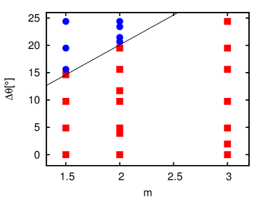
Figure 5: (a) The dimensionless free energy $\Delta\Gamma$ (see Eq. (40)) is shown for the tilted state as well for the upright state for $m=2$. A transition point is found at $\Delta\theta_{t}\approx 20^{\circ}$. For $\Delta\theta<\Delta\theta_{t}$ the tilted state minimizes the free energy. The upright state minimizes the free energy above $\Delta\theta_{t}$.
(b) The regions in the $m$-$\Delta\theta$ phase diagram where the tilted and upright state minimize the free energy are shown by squares and circles, respectively. The black line separates both areas.

Figure 5 shows the dimensionless free energy $\Delta\Gamma$ as a function of $\Delta\theta$ for $m=2$. It compares the values of $\Delta\Gamma$ for the tilted state and the upright state. A transition point is found at $\Delta\theta_{t}\approx 20^{\circ}$. For $\Delta\theta<\Delta\theta_{t}$ the geometry dominates and the upright orientation minimizes the free energy. For larger values of the Janus parameter, the wettability effect dominates and the upright orientation poses the free energy minimum. The phase diagram depending on $\Delta\theta$ and $m$ is shown in Fig. 5. The results are obtained from the simulation of a Janus particle adsorption to a flat interface and Eq. (41). The study is done in the ranges of $0\leq\Delta\theta\leq 25^{\circ}$ and $1.5\leq m\leq 6$. The regions where the shape dominates and is in the tilted state are shown by red squares. The Janus dominated regions with the upright orientation as the free energy minimum are shown by blue circles. For $m\geq 3$ the tilted state is found in the whole simulated region. For smaller aspect ratios transition points are found. The transition value of $\Delta\theta$ increases with an increasing aspect ratio $m$.

V Adsorption trajectories

Finally, we study the trajectories of the adsorption of a single Janus particle to a flat fluid interface. We present three different situations where the interplay between particle shape and wettability difference has a different impact. The three examples differ in the choice of the two parameters $m$ and $\Delta\theta$.

The first situation with the parameters $m=2$ and $\Delta\theta\approx 2^{\circ}$ is presented in Fig. 6. The dashed and dotted lines show the adsorption trajectories for the PIO (“preferred initial orientation”, see Fig. 1) and the UIO (“unpreferred initial orientation”), respectively. The square indicates the ending point of both dashed and dotted lines. The circle and blue triangles show the exclusive end points of dashed and dotted lines, respectively. The solid lines indicate the points where the particle touches the interface. This is the initial condition for the PIO and the UIO as shown in Fig. 1. The Roman numerals relate the points for the final states in Fig. 6 to the sketches in Fig. 6.

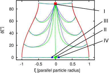
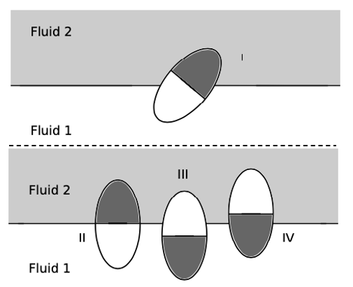
Figure 6: (a) Adsorption trajectories ($\vartheta^{\prime}$-$\xi$-plot) of a single Janus particle at a flat interface for $m=2$ and $\Delta\theta\approx 2^{\circ}$. The dashed and dotted lines represent the trajectories for the PIO and UIO, respectively. The following types of end points or final states (characterized by $\xi$ and $\vartheta^{\prime}$) are shown: The square indicates the end point of both dashed and dotted lines. The circle and triangles show the exclusive end points of dashed and dotted lines, respectively. The Roman numerals relate the points for the final states to the following sketches: (b) Sketch of the tilted state (“I”, $0<\vartheta^{\prime}<90$ and $\xi=0$) corresponding to the square in (a) (upper end point) and the metastable states for different cases of the upright orientation $\vartheta^{\prime}=0$ (“II”). Left particle: every wetting area is immersed completely in its preferred fluid. $\vartheta=0$, $\xi=0$ (related to the circle in (a)). Middle (“III”) and right (“IV”) particle: one wetting area is completely and the other one partly inside its unpreferred fluid. $\vartheta=180^{\circ}$, $\pm\xi_{\rm unpr}$ (related to both triangles in (a) and given in Eq. (42)). The interface is flat for all three final states.

All trajectories with $\vartheta_{0}^{\prime}>0$ end up in a tilted state (as shown by the square in Fig. 6 and state “I” in Fig. 6) characterized by the final position of $\xi_{\rm up}=0$. The final orientation is tilted and close to the parallel orientation found for a particle with a uniformly wetting surface. This is close to the state with the largest interfacial area occupation. The latter was achieved in the case for a uniformly wetting particle, where the particle is oriented parallel to the interface. Even the line of $\vartheta_{0}=(10^{-4})^{\circ}$ ends up in state “I” suggesting the existence of a free energy maximum for Janus particles. This is in agreement with Fig. 5.

For the trajectories of the initial orientation of $\vartheta_{0}^{\prime}=0$, the particle does not rotate, but stays in the upright orientation. One needs to distinguish between the PIO ($\vartheta_{0}=0$) and the UIO ($\vartheta_{0}=180^{\circ}$). In the PIO, the particle ends at the point $\vartheta_{0}^{\prime}=0$ and $\xi_{\rm pr}=0$.This state is indicated by the circle in Fig. 6 and the left particle (state “II”) in Fig. 6. Each wetting area is completely immersed in its preferred fluid and the border between both wetting areas is exactly in contact with the interface. The interface is undeformed in this state. In the UIO, the final position splits as $\pm\xi_{\rm unpr}$ for the two adsorption trajectories coming from both sides of the interface. $\xi_{\rm unpr}$ is the absolute value of the position for the upright orientation in the UIO. For a positive sign of $\xi_{0}$, the particle ends up in a distance of $\xi_{\rm unpr}$ above the interface and for a negative sign of $\xi_{0}$ in a distance of $\xi_{\rm unpr}$ below the interface. This state is indicated by the two triangles in Fig. 6 for both values of $\xi_{\rm unpr}$ and the centered and right particle in Fig. 6. A relation for $\xi_{\rm unpr}$ can be obtained from the geometrical consideration of an ellipsoidal particle as

$$\xi_{\rm unpr}=\frac{mR_{\parallel}\tan(\Delta\theta)}{\sqrt{1+m^{2}\tan^{2}(\Delta\theta)}}\mbox{.}$$ (42)

In this configuration ($\vartheta_{0}=180^{\circ}$ and $\pm\xi_{\rm unpr}$), the Young equation can be fulfilled by a flat fluid interface. In the recent example with $m=2$, $\Delta\theta=1.95^{\circ}$ and $R_{\parallel}=1$ (the latter one due to the fact that $\xi_{\rm unpr}$ is like $\xi$ in units of $R_{\parallel}$), we obtain $\xi_{\rm unpr}=6.8\cdot 10^{-2}$ from Eq. (42). This is close to the value from the simulation $\xi_{\rm unpr}\approx 9.5\cdot 10^{-2}$ (the blue triangle in Fig. 6). The deviation is a result of the discretization of the particle on the lattice.

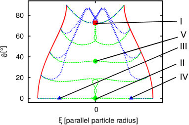
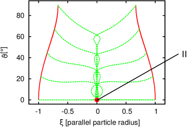
Figure 7: $\vartheta^{\prime}$-$\xi$-plots for the adsorption of a single Janus with different values of $m$ and $\Delta\theta$. Line and end point colors are identical to Fig. 6. The Roman numerals relate the points for the final states in Fig. 6 and Fig. 6. State “V” is a tilted state similar to state “I”, but with a different angle $\vartheta$. (a) ($\Delta\theta\approx 19.5^{\circ}$, $m=2$) The structure of the $\vartheta$-$\xi$ plot is more complicated as compared to Fig. 6. For the PIO, there are two different tilted states. Furthermore, the range of initial orientations for the final upright orientation is extended. (b) ($m=1.5$ and $\Delta\theta\approx 19.5^{\circ}$) Only one final point is there for the upright position $\vartheta_{\rm final}=\vartheta_{\rm upright}=0$ as shown by the left particle in Fig. 6.

Figure 7 shows the adsorption trajectories for $m=2$ and $\Delta\theta\approx 19.5^{\circ}$. The Janus effect is stronger as compared to the previous example. Furthermore, the structure of end points is more complex. Besides the upper point $\vartheta_{\rm up}$ (state “I”) and the upright point $\vartheta_{\rm upright}$ (states “II”, “III” and “IV”), there is an additional end point related to the orientation $\vartheta_{\rm middle}$ (“second tilted orientation”, state “V”). It is a tilted orientation similar to the one of state “I”, but with a different value of the angle. Its value is located between the two other orientations as $\vartheta_{\rm upright}<\vartheta_{\rm middle}<\vartheta_{\rm up}$. The final point of a given adsorption trajectory depends on the initial orientation as follows: for the PIO, the final position is given as $\xi=0$ for all initial orientations. The trajectories for the two upper starting angles ($\vartheta_{0}\geq 67.5^{\circ}$) end up in the upper final point (state “I”). The trajectory of $\vartheta_{0}=45^{\circ}$ ends up (as the only one from the considered initial orientations defined in Eq. (7)) in the “second tilted orientation”. The trajectories for the two lower values of $\vartheta_{0}$ end up in the upright orientation $\vartheta_{\rm upright}$ (state “II”). In contrast to the situation of Fig. 6, there is an extended range of initial orientations which end up finally in the upright orientation.

For the UIO, the ending point structure is completely different from the PIO. The trajectories for the reference orientations $\vartheta_{0}^{\prime}\leq 22.5^{\circ}$ end up in the upper final point. For an initial orientation of $\vartheta_{0}=180^{\circ}$, the particle keeps its orientation during the adsorption process. The position is predicted from Eq. (42) $\xi_{\rm unpr}\approx 5.78\cdot 10^{-1}$ and from the simulation results $\xi_{\rm unpr}=6.22\cdot 10^{-1}$. All UIO trajectories of $\vartheta_{0}\neq 180^{\circ}$ end up in $\xi=0$. Note that state “V” can be found in several regions in the $m$-$\Delta\theta$ diagram. It is shown in the calculations in section IV that there is no region in the $m$-$\Delta\theta$ diagram , where state “V” minimizes the free energy.

A fully Janus dominated case is shown in Fig. 7 for $m=1.5$ and $\Delta\theta\approx 19.5^{\circ}$. All studied trajectories end up in the upright orientation (state “II”). There is no tilted state found for any of the initial orientations. The anisotropy is so weak that the free energy gain due to the excluded interfacial area $A_{ex}$ for a final orientation of $\vartheta>0$ is small. However, the Janus effect ($\Delta\theta$) is sufficiently strong to enforce an orientation where each wetting area is in its preferred fluid.

VI Conclusions

We studied the equilibrium configuration and adsorption process of ellipsoidal Janus particles at a fluid-fluid interface. We presented free energy models with and without consideration of the deformation of the fluid interface and compared the final states of the particle at the fluid interface obtained from the lattice Boltzmann simulations with the predictions from the free energy calculation. The model without interface deformation is only able to predict the simulation results within a specific range, whereas the improved model which takes into account the full rotation of the particle and the deformability of the interface shows a good agreement with our simulation results.

We show that the equilibrium state of a Janus ellipsoid which is determined by the minimum of the free energy is a tilted orientation for large aspect ratios and small wettability differences, where the shape dominates. In case of small aspect ratio and large wettability difference, the Janus effect dominates and the particle is in an upright orientation. Thus, the equilibrium state of an ellipsoidal Janus particle at a fluid interface can be tuned by the choice of aspect ratio and wettability contrast.

Finally, we studied the adsorption trajectories of ellipsoidal Janus particles for three representative cases of the particle aspect ratio and wettability contrast. The interplay of these two parameters does not only influence the final state the sytsem will achieve, but also determines the complex dynamics of the rotation and movement of the particle. Furthermore, we demonstrated that the adsorption trajectory of a symmetric, ellipsoidal Janus particle can show up to three metastable points whereas the uniformly wetting counterpart is known to have only a single metastable point.

- (1) A. Walther and A. Müller. Janus particles: Synthesis, self-assembly, physical properties, and applications. Chem. Rev., 113(7):5194, 2013.
- (2) M. Fernandez-Rodriguez, M. Rodriguez-Valverde, M. Cabrerizo-Vilchez, and R. Hidalgo-Alvarez. Surface activity and collective behaviour of colloidally stable Janus-like particles at the air-water interface. Soft Matter, 10:3471, 2014.
- (3) M. Fernandez-Rodriguez, M. Rodriguez-Valverde, M. Cabrerizo-Vilchez, and R. Hidalgo-Alvarez. Surface activity of Janus particles adsorbed at fluid–fluid interfaces: Theoretical and experimental aspects. Adv. Colloid Interface Sci., 233:240, 2016.
- (4) R. J. Archer, A. J. Parnell, A. I. Campbell, J. R. Howse, and S. J. Ebbens. A pickering emulsion route to swimming active Janus colloids. Adv. Sci., 5:1700528, 2018.
- (5) C. Marschelke, A. Fery, and A. Synytska. Janus particles: from concepts to environmentally friendly materials and sustainable applications. Colloid Polym. Sci., 298:841–865, 2020.
- (6) G. Morris, K. Hadler, and J. Cilliers. Particles in thin liquid films and at interfaces. Curr. Opin. Colloid Interface Sci., 20(2):98, 2015.
- (7) B. Park and D. Lee. Configuration of nonspherical amphiphilic particles at a fluid-fluid interface. Soft Matter, 8:7690, 2012.
- (8) B. Park and D. Lee. Equilibrium orientation of nonspherical Janus particles at fluid–fluid interfaces. ACS Nano, 6(1):782, 2012.
- (9) Y. Hirose, S. Komura, and Y. Nonomura. Adsorption of Janus particles to curved interfaces. J. Chem. Phys., 127(5), 2007.
- (10) B. Binks and P. Fletcher. Particles adsorbed at the oil-water interface: A theoretical comparison between spheres of uniform wettability and Janus particles. Langmuir, 17:4708, 2001.
- (11) H. Fan and A. Striolo. Nanoparticle effects on the water-oil interfacial tension. Phys. Rev. E, 86:051610, 2012.
- (12) A. F. Mejia, A. Diaz, S. Pullela, Y. Chang, M. Simonetty, C. Carpenter, J. D. Batteas, M. S. Mannan, A. Clearfield, and Z. Cheng. Pickering emulsions stabilized by amphiphilic nano-sheets. Soft Matter, 8:10245, 2012.
- (13) H. Rezvantalab and S. Shojaei-Zadeh. Capillary interactions between spherical Janus particles at liquid-fluid interfaces. Soft Matter, 9:3640, 2013.
- (14) C. Anzivino, F. Chang, G. Soligno, R. van Roij, W. K. Kegel, and M. Dijkstra. Equilibrium configurations and capillary interactions of Janus dumbbells and spherocylinders at fluid–fluid interfaces. Soft Matter, 15:2638–2647, 2019.
- (15) Q. Xie and J. Harting. Controllable capillary assembly of magnetic ellipsoidal Janus particles into tunable rings, chains and hexagonal lattices, 2020.
- (16) S. Frijters, F. Günther, and J. Harting. Effects of nanoparticles and surfactant on droplets in shear flow. Soft Matter, 8:6542, 2012.
- (17) F. Günther, F. Janoschek, S. Frijters, and J. Harting. Lattice Boltzmann simulations of anisotropic particles at liquid interfaces. Comput. Fluids, 80:1840, 2012.
- (18) T. Krüger, S. Frijters, F. Günther, B. Kaoui, and J. Harting. Numerical simulations of complex fluid-fluid interface dynamics. Eur. Phys. J. Spec. Top., 222(1):177, 2013.
- (19) F. Günther, F. Janoschek, S. Frijters, and J. Harting. Lattice Boltzmann simulations of anisotropic particles at liquid interfaces. Comp. Fluids, 80(0):184, 2013.
- (20) F. Günther, S. Frijters, and J. Harting. Timescales of emulsion formation caused by anisotropic particles. Soft Matter, 10(27):4977–4989, 2014.
- (21) F. Günther, S. Frijters, and J. Harting. Timescales of emulsion formation caused by anisotropic particles. Soft Matter, 10:4977, 2014.
- (22) S. Succi. The Lattice Boltzmann Equation for Fluid Dynamics and Beyond. Numerical Mathematics and Scientific Computation. Oxford University Press, Oxford, 2001.
- (23) P. Bhatnagar, E. Gross, and M. Krook. A model for collision processes in gases. I. Small amplitude processes in charged and neutral one-component systems. Phys. Rev., 94:511, 1954.
- (24) X. Shan and H. Chen. Lattice Boltzmann model for simulating flows with multiple phases and components. Phys. Rev. E, 47:1815, 1993.
- (25) F. Jansen and J. Harting. From bijels to Pickering emulsions: A lattice Boltzmann study. Phys. Rev. E, 83:046707, 2011.
- (26) C. Aidun, Y. Lu, and E. Ding. Direct analysis of particulate suspensions with inertia using the discrete Boltzmann equation. J. Fluid Mech., 373:287, 1998.
- (27) A. Ladd. Numerical simulations of particulate suspensions via a discretized Boltzmann equation. Part I. Theoretical foundation. J. Fluid Mech., 271:285, 1994.
- (28) A. Ladd. Numerical simulations of particulate suspensions via a discretized Boltzmann equation. Part II. Numerical results. J. Fluid Mech., 271:311, 1994.
- (29) A. Ladd and R. Verberg. Lattice-Boltzmann simulations of particle-fluid suspensions. J. Stat. Phys., 104:1191, 2001.
- (30) A. Komnik, J. Harting, and H. J. Herrmann. Transport phenomena and structuring in shear flow of suspensions near solid walls. J. Stat. Mech.: theory and experiment, P12003, 2004.
- (31) D. Stamou, C. Duschl, and D. Johannsmann. Long-range attraction between colloidal spheres at the air-water interface: The consequence of an irregular meniscus. Phys. Rev. E, 62:5263, Oct 2000.
- (32) H. Lehle, E. Noruzifar, and M. Oettel. Ellipsoidal particles at fluid interfaces. Eur. Phys. J. E, 26:151, 2008.
- (33) J. Loudet, A. Alsayed, J. Zhang, and A. Yodh. Capillary interactions between anisotropic colloidal particles. Phys. Rev. Lett., 94:018301, 2005.
- (34) J. Bleibel, A. Domínguez, and M. Oettel. Colloidal particles at fluid interfaces: Effective interactions, dynamics and a gravitation–like instability. Eur. Phys. J. Spec. Top., 222(11):3071, 2013.
- (35) M. Oettel and S. Dietrich. Colloidal interactions at fluid interfaces. Langmuir, 24(4):1425, 2008.
- (36) A. Kumar, B. Park, F. Tu, and D. Lee. Amphiphilic Janus particles at fluid interfaces. Soft Matter, 9:6604, 2013.
- (37) H. Rezvantalab and S. Shojaei-Zadeh. Role of geometry and amphiphilicity on capillary-induced interactions between anisotropic Janus particles. Langmuir, 29(48):14962, 2013.