Numerical approximations of chromatographic models

Abstract.

A numerical scheme based on modified method of characteristics with adjusted advection (MMOCAA) is proposed to approximate the solution of the system liquid chromatography with multi components case. For the case of one component, the method preserves the mass. Various examples and computational tests numerically verify the accuracy and efficiency of the approach.

Keywords: Advection-Diffusion, Coupled system, Langmuir adsorption model, Liquid Chromatography, Numerical approximation.
2010 MSC:

1. Introduction and problem setting

Chromatography is a technical process to separate mixed chemical components with a wide range of chemical industrial applications such as in pharmaceutical, food ingredients, etc. Here, we briefly explain the separation of components by liquid chromatography. In column chromatography a mixed sample is injected into a fluid stream which is called mobile phase. Then the fluid is pumped through a pipe which we refer as chromatographic column. The column is filled with very small porous beads called stationary phase. Different components in fluid adsorbs and/or desorbs at different rates on the stationary phase so they move through the column at different speeds and exit the column at different times; elution, see [6, 9].

The transport of solutes in heterogeneous porous media is described by mass balance equation. The transport is influenced by the convection, diffusion, dispersion and also reaction/adsorption between solute and the porous environment. The model consists of system of convection-diffusion-reaction partial differential equations with dominating the convective terms coupled via differential or algebraic equations. To see different models and numerical approach, we refer to [9].

2. Preliminaries and Problem setting

In one-dimension, the transport is given by the following coupled equations:

(2.1) $$\left\{\begin{array}[]{ll}\frac{\partial u_{i}}{\partial t}+F\,\frac{\partial q_{i}}{\partial t}+v\frac{\partial u_{i}}{\partial x}=D\,\frac{\partial^{2}u_{i}}{\partial x^{2}}&\text{in }(0,L)\times(0,T),\\ \\ u_{i}(x=0,t)=g_{i}(t)&\text{on }(0,T),\\ \\ u_{i}(x,t=0)=u_{i,0}(x)&\text{in }(0,L),\\ \\ \frac{\partial u_{i}(x=L,t)}{\partial x}=0&\text{for }t\geq 0,\\ \\ i=1,2,\cdots m,\end{array}\right.$$

where,

• $L:$ the column length,

• $t:$ time,

• $u_{i}:$ concentration of the $i^{\rm{th}}$ component in the mobile phase,

• $q_{i}:$ concentration of the $i^{\rm{th}}$ component in the stationary phase,

• $u_{i,0}:$ initial condition,

• $g_{i}:$ boundary condition (injection profile),

• $F:$ stationary/mobile phase ratio,

• $v:$ mobile phase velocity,

• $D:$ diffusion parameter,

• $m:$ number of mixture components in the sample.

The Neumann boundary condition $\frac{\partial u_{i}(x=L,t)}{\partial x}=0$ persuade continuity of the outlet concentration profile to the connecting tube receiving the fluid after leaving the column. The dispersion coefficient $D$ is given by

$$D=\frac{L\,v}{2N_{t}},$$

where $N_{t}$ is the number of theoretical plates. The term $F$ is given by

$$F=\frac{1-\epsilon}{\epsilon},$$

which indicates the phase ratio based on the porosity $\epsilon$. Also $q_{i}$ is called adsorption isotherm and we assume that $q_{i}=q_{i}(u_{1},\cdots,u_{m})$. In Langmuir model this term is given by

(2.2) $$q_{i}=\frac{a_{i}u_{i}}{1+\sum\limits_{j=1}^{m}b_{j}u_{j}},\quad i=1,2,\cdots m,$$

where $a_{i},b_{i}>0$.

Let assume that the mass of components at the initial time in column is zero; $u_{i,0}(x)=0,\,\,\,\,0<x<L$. We consider rectangular injection profiles so boundary condition at the inlet point is:

$$u_{i}(x=0,t)=g_{i}(t)=u_{i,\textrm{inj}}(t),$$

with

(2.3) $$u_{i,\textrm{inj}}(t)=\left\{\begin{array}[]{ll}u_{i,f}(t)&0<t\leq t_{\textrm{inj}},\\ 0&t>t_{\text{inj}},\end{array}\right.$$

where $u_{i,f}(t)$ is the inlet feed concentration and $t_{\text{inj}}$ is the injection time. One can consider Danckwerts-type boundary conditions at the column inlet which is given by,

$$u_{i}(x=0,t)=u_{i,\textrm{inj}}(t)+\frac{D}{v}\,\frac{\partial u_{i}}{\partial x}\quad i=1,\cdots,m,$$

where for $N_{t}>100$, e.g. Seidel-Morgenstern [20], it reduces again to

$$u_{i}(x=0,t)=u_{i,\text{inj}}(t).$$

It is well known that in the convection dominate problems, discontinuity propagates in time even with the smooth initial and boundary data. Furthermore, the nonlinearity and coupling in term $q_{i}$ in (2.1) brings more challenges to the numerical solution of this type of nonlinear coupled convection-diffusion system.

Standard finite difference, finite volume, and finite element methods are not stable and the numerical approximations exhibit non-physical oscillations and/or generates artificial numerical diffusion, which smear out sharp fronts of the solution [7, 8, 16].

In the case of scalar equation, one approach to eliminate the nonphysical oscillation which occurs on standard finite element or finite difference approach, is based on characteristic method. The sketch of idea is splitting the equation into two sub-steps, the convection step, which is solved explicitly by high order schemes (Lax Wendroff for instance), and the diffusion step, which is solved implicitly by central difference, see [1, 3].

For the system (2.1), different approaches have been discussed. In [10] high resolution semi-discrete flux-limiting finite volume scheme is proposed which is capable to defeat numerical oscillations and preserves the positivity of numerical solution. The authors validate their scheme against other flux-limiting schemes available in the literature. To see about discontinuous Galerkin approximation for system (2.1) we refer to [11, 14, 15]. Recently in [19] a transport model is used to describe gradient elution in liquid chromatography. Furthermore, the authors implement Laplace transform to obtain the analytical solution of model.

In [2] the existence of the unique weak solution has shown for the case that $q=\nabla\phi$ for some $\phi:\mathbb{R}^{m}\rightarrow\mathbb{R}$, i.e the vector field $q:\mathbb{R}^{m}\rightarrow\mathbb{R}^{m}$ in (2.1) can be expressed as a gradient of some non-negative $C^{1}$-convex function $\phi$. The proof is based on Rothe’s method along with solving a convex minimization problem at each time step which gives a numerical method to solve the coupled system.

We propose the modified method of characteristics with adjusted advection (MMOCAA) to solve the system of equation (2.1). This method was proposed by Douglas et al. to solve advection dominate transport PDEs [3]. The MMOCAA corrects the mass error occurs in the modified method of characteristic (MMOC) by perturbing the foot of the characteristics vaguely [4, 17]. Our method is straight forward to implement and robust comparing the other methods mentioned above. Error analysis for presented scheme is beyond our aim in the current work.

The paper is organized as follows. Section 2 deals with introducing problem and previous works. In Section 3 we present our numerical scheme for coupled system and for scalar equation in ideal case. We finally represent various examples and computational tests.

3. The numerical scheme

For the sake of simplicity, let’s assume that the number of components is two ($m=2$) however, it can simply extended for $m>2$.

(3.1) $$\left\{\begin{array}[]{ll}\frac{\partial u_{1}}{\partial t}+F\frac{\partial q_{1}}{\partial t}+v\,\frac{\partial u_{1}}{\partial x}=D\,\frac{\partial^{2}u_{1}}{\partial x^{2}}&\text{in }(0,L)\times(0,T),\\ \\ \frac{\partial u_{2}}{\partial t}+F\frac{\partial q_{2}}{\partial t}+v\,\frac{\partial u_{2}}{\partial x}=D\,\frac{\partial^{2}u_{2}}{\partial x^{2}}&\text{in }(0,L)\times(0,T),\\ \\ u_{k}(x=0,t)=g_{i}(t),\quad k=1,2&\text{on }(0,T),\\ \\ u_{k}(x,t=0)=0,\,\quad\quad k=1,2&\text{in }(0,L),\\ \\ \frac{\partial u_{1}(x=L,t)}{\partial x}=0,\frac{\partial u_{2}(x=L,t)}{\partial x}=0&\text{for }t\geq 0.\end{array}\right.$$

We start semi-discritization in time for system (3.1). For positive integer number $N$, the time interval $[0,T]$ is divide to $N$ sub interval as

(3.2) $$[0,T]=[t^{0},t^{1}]\cup\dots\cup[t^{N-1},t^{N}],$$

where $t^{n}=n\triangle t,n=1,\dots,N$ and $\triangle t=\frac{T}{N}$.

Let $u_{k}^{n}(x):=u_{k}(t^{n},x)$. If we start form the point $(x_{i},t^{n+1})$ and move back in direction of characteristic line, then we hit the time level $n$. The intersection point is called $(\tilde{x}_{i},t^{n})$.

By method of characteristic we have

$$u_{k}(x_{i},t^{n+1})=\tilde{u}_{k}^{n}(\tilde{x}_{i}):=u_{k}^{n}(x_{i}-v\,\triangle t),\quad\text{for}\,k=1,2.$$

As $\tilde{x}_{i}$ may not be a grid point, $\tilde{u}_{i}^{n}(\tilde{x}_{i})$ is an interpolated value. For $v\,\frac{\triangle t}{\triangle x}<1,$ the foot of backward characteristic $\tilde{x}_{i}$ intersects $t=t^{n}$ inside the interval $(x_{i-1},x_{i+1}).$ We can use quadratic interpolation between $u_{i-1}^{n},u_{i}^{n},u_{i+1}^{n}$ which leads to the Lax-Wendrof scheme in the scalar case.

By using the chain rule, we have

$$\frac{\partial q_{1}}{\partial t}=\frac{\partial q_{1}}{\partial u_{1}}\,\frac{\partial u_{1}}{\partial t}+\frac{\partial q_{1}}{\partial u_{2}}\,\frac{\partial u_{2}}{\partial t}.$$

We use the notation $\mathbf{u}(\cdot,t^{n})=\mathbf{u}^{n}(\cdot).$ To update the values of $\mathbf{u}=(u_{1},u_{2})$ at the point $(x_{i},t^{n+1}),$ we follow backward in the direction of the characteristic line. The semi-discretization of (3.1) reads as follows

(3.3) $$\frac{u_{1}^{n+1}-\widetilde{u_{1}}^{n}}{\triangle t}+F\,\frac{\partial q_{1}^{n}}{\partial u_{1}}\,\frac{u_{1}^{n+1}-u_{1}^{n}}{\triangle t}+F\,\frac{\partial q_{1}^{n}}{\partial u_{2}}\,\frac{u_{2}^{n+1}-u_{2}^{n}}{\triangle t}=D(u_{1}^{n+1})_{xx},$$

(3.4) $$\frac{u_{2}^{n+1}-\widetilde{u_{2}}^{n}}{\triangle t}+F\,\frac{\partial q_{2}^{n}}{\partial u_{1}}\,\frac{u_{1}^{n+1}-u_{1}^{n}}{\triangle t}+F\,\frac{\partial q_{2}^{n}}{\partial u_{2}}\,\frac{u_{2}^{n+1}-u_{2}^{n}}{\triangle t}=D(u_{2}^{n+1})_{xx}.$$

The iterative methods in (3.3) and (3.4) can be reformulated as

$$\frac{\mathbf{u}^{n+1}-\widetilde{\mathbf{u}}^{n}}{\triangle t}+F\,\mathbf{A}^{n}\frac{{\mathbf{u}}^{n+1}-\mathbf{u}^{n}}{\triangle t}=D\mathbf{u}_{xx}^{n+1},$$

where

$$\mathbf{u}^{n}(x)=\left(\begin{array}[]{cc}u_{1}^{n}(x)\\ u_{2}^{n}(x)\\ \end{array}\right)\quad\text{and}\quad\quad\mathbf{A}^{n}=\left(\begin{array}[]{cc}\frac{\partial q_{1}^{n}}{\partial u_{1}}&\frac{\partial q_{1}^{n}}{\partial u_{2}}\\ \\ \frac{\partial q_{2}^{n}}{\partial u_{1}}&\frac{\partial q_{2}^{n}}{\partial u_{2}}\\ \end{array}\right).$$

Note that $\frac{\partial q_{1}}{\partial u_{1}}$,$\frac{\partial q_{1}}{\partial u_{2}}$, $\frac{\partial q_{2}}{\partial u_{1}}$ and $\frac{\partial q_{2}}{\partial u_{2}}$, are evaluated at the previous time step ($t=t_{n}$). In order to improve the approximation of (3.3) and (3.4) we use the following iteration

(3.5) $$\frac{u_{1,l}^{n+1}-\widetilde{u_{1}}^{n}}{\triangle t}+F\,\frac{\partial q_{1,l-1}^{n}}{\partial u_{1}}\,\frac{u_{1,l}^{n+1}-u_{1}^{n}}{\triangle t}+F\,\frac{\partial q_{1,l-1}^{n}}{\partial u_{2}}\,\frac{u_{2,l}^{n+1}-u_{2}^{n}}{\triangle t}=D(u_{1,l}^{n+1})_{xx},$$

(3.6) $$\frac{u_{2,l}^{n+1}-\widetilde{u_{2}}^{n}}{\triangle t}+F\,\frac{\partial q_{2,l-1}^{n}}{\partial u_{1}}\,\frac{u_{1,l}^{n+1}-u_{1}^{n}}{\triangle t}+F\,\frac{\partial q_{2,l-1}^{n}}{\partial u_{2}}\,\frac{u_{2,l}^{n+1}-u_{2}^{n}}{\triangle t}=D(u_{2,l}^{n+1})_{xx},$$

where

$$\frac{\partial q_{1,l}^{n}}{\partial u_{1}}=\frac{q_{1}(u^{n+1}_{1,l},\cdot)-q_{1}(u_{1}^{n},\cdot)}{u_{1,l}^{n+1}-u^{n}_{1}}.$$

To keep the mass preserved in the scheme, we follow the idea of adding perturbation, see[10]. Define two perturbations of $x_{f}$ by

$$x^{+}_{f}=x_{i}-v\,\triangle t+\eta\triangle t\,\triangle x,$$

$$x^{-}_{f}=x_{i}-v\,\triangle t-\eta\triangle t\,\triangle x,$$

where the constant $0<\eta<1$ depends on $D$, $u$, $\triangle t$ and $\triangle x$. After computing the values $u_{+}^{n}=u^{n}(x^{+}_{f})$ and $u_{-}^{n}=u^{n}(x^{-}_{f})$ we can compare the amount of injected concentration for each of components (plus initial concentration if it is not zero) with the approximated solution until level $n$. If the approximated mass accumulated up to time level $n$ be less than injected mass, set:

$$u^{n}=\max(u_{+}^{n},u_{-}^{n}),$$

otherwise,

$$u^{n}=\min(u_{+}^{n},u_{-}^{n}).$$

Remark 3.1.

One can easily derive the weak formulation and semi-discretized system and do simulation based on that.

(3.7) $$\begin{split}\left\langle\mathbf{u}^{n}-\tilde{\mathbf{u}}^{n-1},\boldsymbol{\phi}\right\rangle+\left\langle\nabla_{u}\mathbf{q}^{n}\,(\mathbf{u^{n}}-\mathbf{u^{n-1}}),\boldsymbol{\phi}\right\rangle+\triangle t\,\left\langle\nabla\mathbf{u}^{n},\nabla\boldsymbol{\phi}\right\rangle+\triangle t\,\left\langle\nabla\mathbf{u}^{n},{\phi}\right\rangle&=\\ \triangle t\,\left\langle\mathbf{g}(t^{n},\mathbf{u}^{n-1}),\boldsymbol{\phi}\right\rangle.&\end{split}$$

where

(3.8) $$\mathbf{u}^{n}(x):=\begin{pmatrix}u_{1}^{n}(x)\\ u_{2}^{n}(x)\end{pmatrix}.$$

3.1. Ideal model

In the ideal model, we assumes that axial dispersion is negligible i.e., $D=0$ which means that the column has an infinite efficiency and the thermodynamic equilibrium is achieved instantaneously.

3.1.1. Numerical approach

We can use MMOCAA explained in the previous section for the ideal case, i.e, $D=0$. Here, we present a different approach that can be used for one ideal component ($m=1$), i.e.,

$$\frac{\partial{u}}{\partial t}+F\frac{\partial}{\partial t}(\frac{au}{1+bu})+v\frac{\partial{u}}{\partial x}=0.$$

Consider the change of variable

(3.9) $$w=u+F\frac{au}{1+bu}.$$

The idea is to obtain the approximation of $w$ at point $(x_{i},t^{n+1})$. Then $u$ can be recovered as function of $w$ by the following equation

$$u=\frac{-(Fa+1-b\,w)+\sqrt{(Fa+1-b\,w)^{2}+4bw}}{2b}.$$

By Taylor’s expansion we have

(3.10) $$w(x_{i},t^{n+1})=w(x_{i},t^{n})+\triangle t\,w_{t}(x_{i},t^{n})+\frac{(\triangle t)^{2}}{2}w_{tt}(x_{i},t^{n})+O(\triangle t)^{3}.$$

Next we obtain approximation for $w_{t}(x_{i},t^{n})$ and $w_{tt}(x_{i},t^{n}).$ To do so, equation (3.9) implies that:

(3.11) $$w_{t}=(1+\frac{F\,a}{(1+bu)^{2}})\,u_{t}.$$

By taking derivative with respect to $t$ from

(3.12) $$w_{t}=-v\,u_{x}$$

and under some regularity assumption we obtain:

$$w_{tt}=(-v\,u_{x})_{t}=-v\,(u_{t})_{x}.$$

From (3.11) one has

$$u_{t}=\frac{w_{t}}{1+\frac{Fa}{(1+bu)^{2}}}=-\frac{v\,u_{x}}{1+\frac{Fa}{(1+bu)^{2}}}.$$

Next we have

$$(u_{t})_{x}=-v(\frac{u_{x}}{1+\frac{Fa}{(1+bu)^{2}}})_{x}=-\frac{v\,u_{xx}}{1+\frac{Fa}{(1+bu)^{2}}}-2v\frac{Fab(1+bu)u_{x}^{2}}{((1+bu)^{2}+Fa)^{2}}.$$

The recent relation yields

$$w_{tt}=\frac{v^{2}\,u_{xx}}{1+\frac{Fa}{(1+bu)^{2}}}+2v^{2}\frac{Fab(1+bu)u_{x}^{2}}{((1+bu)^{2}+Fa)^{2}}.$$

We can substitute $w_{t}$ and $w_{tt}$ in (3.10) to obtain approximations for $w(x_{i},t^{n+1})$ as below:

(3.13) $$w_{i}^{n+1}=w_{i}^{n}-\frac{v}{2}\frac{\Delta t}{\Delta x}\delta_{x}u_{i}^{n}+\frac{v^{2}}{2}(\frac{\Delta t}{\Delta x})^{2}\big{(}\frac{\delta^{2}_{x}u_{i}^{n}}{1+\frac{Fa}{(1+bu_{i}^{n})^{2}}}+\frac{2Fab\,(1+bu_{i}^{n})(\delta_{x}u_{i}^{n})^{2}}{((1+bu_{i}^{n})^{2}+Fa)^{2}}\big{)},$$

where $\delta_{x}$ is the first central difference operator, $\delta^{2}_{x}$ is the second central difference operator, and $\Delta t$ and $\Delta x$ are the mesh-spacing in $t$ and $x$, respectively. The $i$ and $n$ are space and time indices, and $u_{i}^{n}$ is the grid function such that $u_{i}^{n}=u(x_{i},t_{n})$.

4. Numerical implication

In this section our scheme is validated with different tests. For scalar equation there exist many approaches with different flux limiters: Koren, Von leer, superbee, Minmod, Mc. For more detail about this methods refer to [10]

Example 4.1.

To obtain accuracy and compare with analytical solution we consider the linear adsorption $q=au.$ The analytical solution of this case with linear adsorption with the parameters given in table 1 is derived in [18].

Table 1. Simulation parameters for the linear case study

parameters	Symbols	Values	unite
Column length	$L$	1	cm
Porosity	$F$	1.5	-
Interstitial velocity	$v$	1	cm/min
Henry’s constant	$a$	1	-
constant in adsorption	$b$	0	L/mol
Initial concentration	$u_{0}$	0	mol/L
Feed concentration	$u_{\rm{inj}}$	1	mol/L
Injection time	$t_{\rm{inj}}$	3	min
Simulation time	$t_{\rm{max}}$	7	min

Figure 1 shows both analytical solution and approximated solution with the numbers of spatial steps $n_{x}=100$ and of temporal steps $n_{t}=400$.

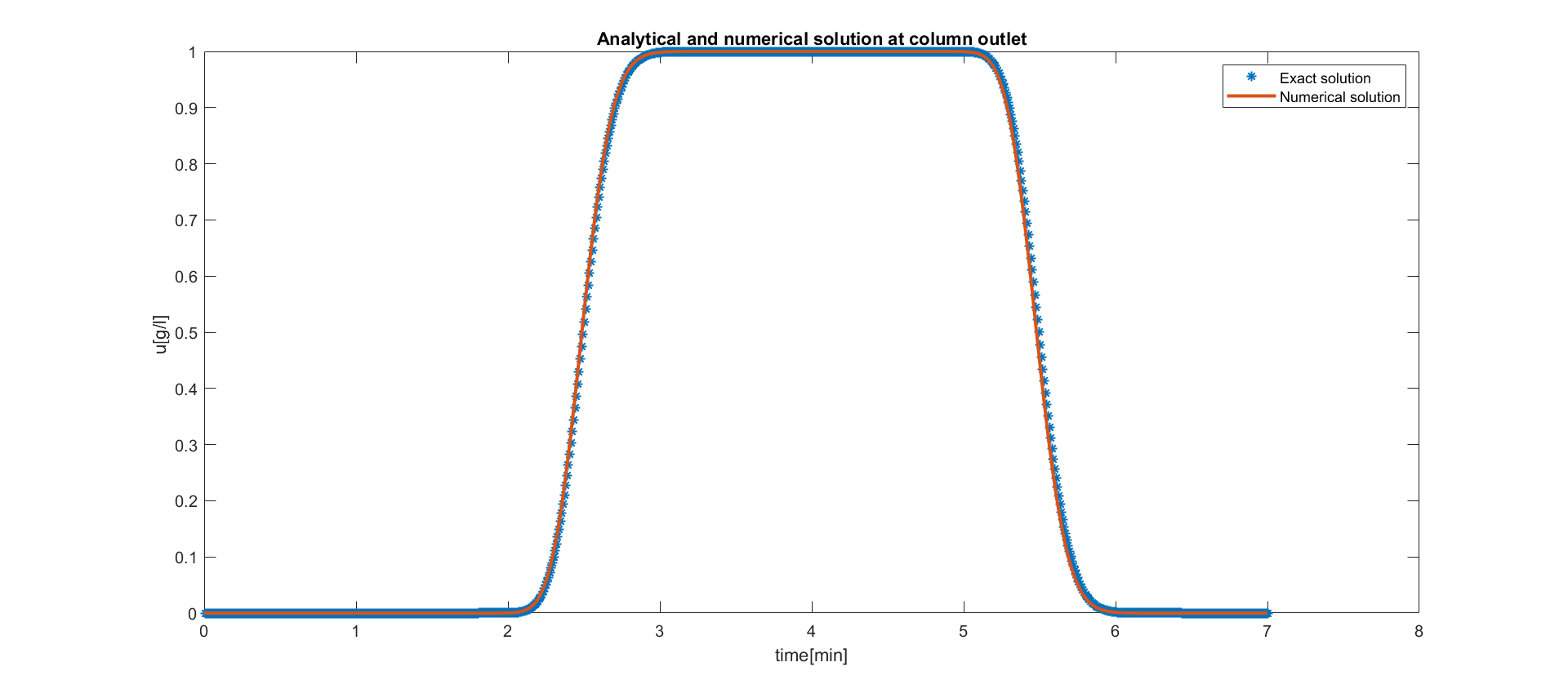
Figure 1. Comparison between analytical(continuous red line) and approximated solutions at outlet (denoted by $\ast$).

Table 2 gives a comparison of $L^{1}$-error and CPU time of our method with discontinuous Galerkin finite element method (DG-FE) with linear basis functions in [10, 11] and with high order basis function of order 8 from [14].

Different methods	DOFs	$L^{1}$ error	CPU time(s)
DG-FM(ord=1)	16,000	$0.6\times 10^{-6}$	8827
DG-FM(ord=8)	90	$0.6\times 10^{-6}$	0.7
MMOCAA	100	$0.15\times 10^{-1}$	0.11

Table 2. The comparison of the method used in [14] with MMOCAA

The $L^{1}$-norm of error and CPU time are presented in Table 3.

$n_{x}$	$n_{t}$	$L^{1}$ error	CPU time(s)
$50$	$200$	$0.3\times 10^{-1}$	$0.0703$
$100$	$400$	$0.15\times 10^{-1}$	$0.11$
$200$	$800$	$0.11\times 10^{-1}$	$0.42$
$400$	$1600$	$0.7\times 10^{-2}$	$2.96$
$800$	$3200$	$0.5\times 10^{-2}$	$17.64$

Table 3. $L^{1}$-norm and cpu time for different $n_{x}$ and $n_{t}$.

Example 4.2.

Here we consider the one component model with nonlinear isotherm given as

$$q(u)=\frac{u}{1+u}.$$

The injection time is $0.2$ and a rectangular pulse of hight $1\,g/l$ is injected at inlet. The length of column is $1\textrm{cm,}$ the velocity $v=1\,\textrm{cm/min}$, $\epsilon=.5.$ and $N_{t}=250.$ Figure 2 shows the numerical simulation at outlet, compare with [11].

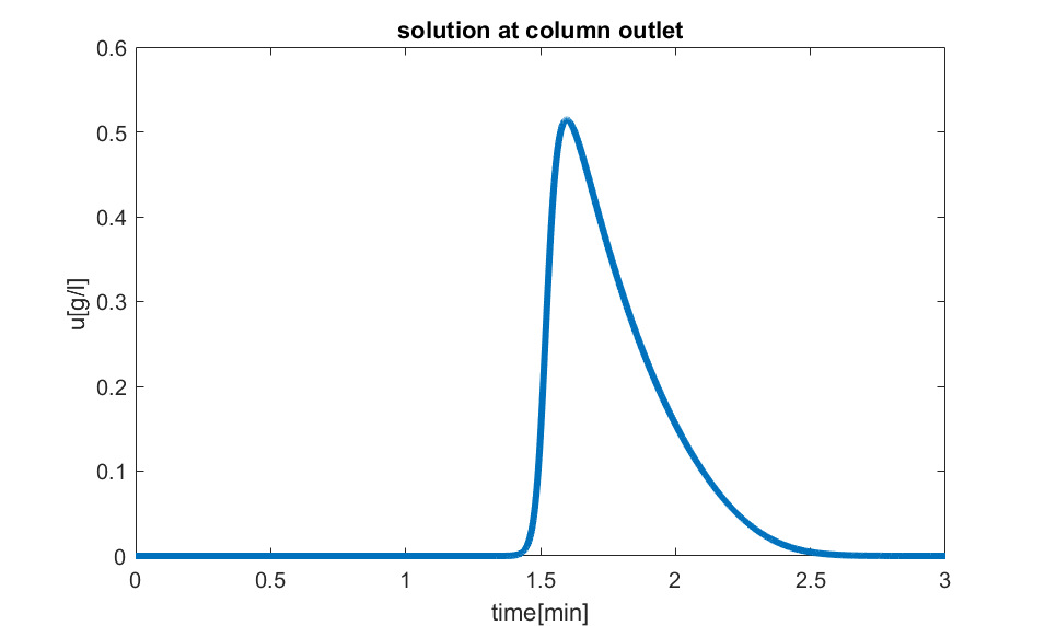
Figure 2. Profile of solution $u$ at outlet $x=1$.

We can calculate the mass injected at the inlet during simulation time. Next, we compute the value of mass passing throughout each points for the time of simulation. Figure 3 indicates that the mass is preserved.

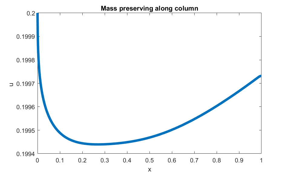
Figure 3. The values of approximated solution at different points in column.

Because there is no analytical solution for this equations as reference solution, we consider $n_{x}=3000$ grid points and $n_{t}=20000$. compare the result with the one in [10]. The $L^{1}$ error and CPU time are recorded in Table 4. We compare the results for the case of $n_{x}=50$ grid points.

Different methods	$L^{1}$ error	CPU time(s)
First order	$0.1146$	0.43
Korren	0.0497	0.56
Van Leer	0.0586	0.56
Superbee	0.0582	0.88
Minmod	0.0645	1.45
MC	0.580	0.62
Our approximation	$0.0014$	$1.5$

Table 4. The comparison of the method used in [10] with our approximate solution for one component nonlinear problem

Example 4.3.

In this example, we compare our simulation with the test given in [14], section 4.22. The parameters are chosen from Table 5 with $N_{t}$= 5000. Here the number of components is two; $m=2$, however, there is no limitation to simulate with even larger numbers of theoretical plates. Figure 4 depicts numerical approximation for two components at outlet $x=1$. See Table 6 for $L^{1}$ error and cpu time.

Table 5. Simulation parameters for the nonlinear case study

Parameters	Symbols	Values	unite
Column length	$L$	1	m
Porosity	$\epsilon$	0.4	-
Interstitial velocity	$v$	0.1	m/s
Henry’s constant	$a_{1},a_{2}$	0.5, 1	-
Constant in adsorption	$b_{1},b_{2}$	.05, 0.1	L/mol
Initial concentration	$u_{1,0},u_{2,0}$	0, 0	mol/L
Feed concentration	$c_{f_{1}},c_{f_{2}}$	10, 10	mol/L

Figure 4. Approximate solution for two components at outlet during simulation time.

Different methods	$L^{1}$ error	CPU time(s)
DG-FM(ord=8)	$0.009$	4.6
Our approximation	$0.05$	2.3

Table 6. The comparison with DG-FM in [14]

References

- [1] L. Baňas, Solution of convection-diffusion equation by the method of characterestics. Journal of Computational and Applied Mathematics, (2004) pp. 31-39.
- [2] M. Baía, F. Bozorgnia, L. Monsaingeon and J. Videman, A degenerate elliptic-parabolic system arising in competitive contaminant transport. J. Math. Anal. Appl, 457(2018) pp. 77–103.
- [3] J. Douglas, J Huang and F. Pereira, The modified method of characteristics with adjusted advection. Numer. Math., (1999) pp.353-369.
- [4] J. Douglas Jr., F. Furtado, F. Pereira,On the numerical simulation of waterflooding of heterogeneous petroleum reservoirs Comput. Geosci., (1997) pp.155–190.
- [5] E. Godlewski, P.A. Raviart, Numerical Approximation of Hyperbolic Systems of Conservation Laws. Applied Mathematical Sciences, Springer, 1991.
- [6] G. Guiochon, Preparative liquid chromatography. Journal of Chromatography A., 965, (2002) pp. 129-161.
- [7] G. Guiochon, G. Shirazi, M. Katti, Fundamentals of preparative and nonlinear chromatography (2nded.) (2006), Elsevier,Inc.
- [8] H. Holden, K.H. Karlsen, K. A. Lie, N. H. Risebro, Splitting Methods for Partial Differential Equations with Rough Solutions: Analysis and MATLAB Programs. European Mathematical Society, 2010.
- [9] S. Javeed, Analysis and Numerical Investigation of Dynamic Models for Liquid Chromatography. PhD thesis, 2013. https:pure.mpg.derestitemsitem-1896908-4componentfile-2028709content.
- [10] S. Javeed, S. Qamar, A. Seidel-Morgenstern and G. Warnecke, Efficient and accurate numerical simulation of nonlinear chromatographic processes Comput. Chem. Eng., 35 (11) (2011) pp. 2294-2305.
- [11] S. Javeed, S. Qamar, A. Seidel-Morgenstern and G. Warnecke, A discontinuous Galerkin method to solve chromatographic models. J. Chromatogr. A., 1218 (2011) pp. 7137-7146.
- [12] S. Javeed, S. Qamar, W. Ashraf, G. Warnecke, and A. Seidel-Morgenstern, Analysis and numerical investigation of two dynamic models for liquid chromatography. Chem. Eng. Sci., 90, (2013) pp. 17-31.
- [13] B. Koren, A robust upwind discretization method for advection, diffusion and source terms. In C. B. Vreugdenhil, B. Koren (Eds.), Numerical methods for advection-diffusion problems, Volume 45 of Notes on Numerical Fluid Mechanics (pp. 117–138). Braunschweig: Vieweg Verlag.
- [14] K. Meyer, J.K Huusom, J. Abildskov, High-order approximation of chromatographic models using a nodal discontinuous Galerkin approach. Computers and Chemical Engineering., 109, (2018) pp. 68-76.
- [15] K. Meyer, J.K Huusom, J. Abildskov, A stabilized nodal spectral solver for liquid chromatography models. Computers and Chemical Engineering., Volume 124, (2019), pp. 172-183.
- [16] P. Rouchon, M. Schonauer, P. Valentin, G. Guiochon, Numericalsimulation of band propagation in nonlinear chromatography. Separation Scienceand Technology., 22, (1987) pp. 1793-1833.
- [17] R. E. Ewing, H. Wang, A summary of numerical methods for time-dependent advection-dominated partial differential equations. J. Comput. Appl. Math., 128 (2001), pp. 423-445.
- [18] S. Qamar, J. N. Abbasi, S. Javeed, M. Shah, F. U. Khan and A. Seidel-Morgenstern, Analytical solutions and moment analysis of chromatographic models for rectangular pulse injections. Journal of Chromatography A, 1315, (2013) pp. 92– 106.
- [19] S. Qamar, N. Rehman, G. Carta, A. Seidel-Morgenstern, Analysis of gradient elution chromatography using the transport model. Chemical Engineering Science, 225, (2020), 115809.
- [20] A. Seidel-Morgenstern, Analysis of boundary conditions in the axial dispersion model by application of numerical laplace inversion. Chemical Engineering Science., Vol. 46, Issue 10, (1991) pp. 2567-2571.