On the probability that a binomial variable is at most its expectation

Abstract.

Consider the probability that a binomial random variable Bi$(n,m/n)$ with integer expectation $m$ is at most its expectation. Chvátal conjectured that for any given $n$, this probability is smallest when $m$ is the integer closest to $2n/3$. We show that this holds when $n$ is large.

1. Introduction

Consider the probability $\operatorname{\mathbb{P}{}}\bigl{(}\operatorname{Bi}(n,p)\leqslant np\bigr{)}$ that a binomial random variable $\operatorname{Bi}(n,p)$ is less that or equal to its mean. (We slighly abuse notation, and let $\operatorname{Bi}(n,p)$ denote both the binomial distribution and a binomial random variable.) By the central limit theorem, unless $n$ or $p(1-p)$ is small, this probability is close to $\frac{1}{2}$; in fact, the Berry–Esseen theorem [2] and [5] (see also e.g [8, Theorem 7.6.1]) shows that $\operatorname{\mathbb{P}{}}(\operatorname{Bi}(n,p)\leqslant np)=\frac{1}{2}+O\bigl{(}(np(1-p))^{-1/2}\bigr{)}$. (See also the explicit bounds in [4], [7], [14], [16], [17].)

In the case when $np=m$ is an integer, Neumann [12] showed that the mean $np$ is also a (strong) median, i.e,

$$\operatorname{\mathbb{P}{}}(\operatorname{Bi}(n,p)<np)<\frac{1}{2}<\operatorname{\mathbb{P}{}}(\operatorname{Bi}(n,p)\leqslant np),\qquad np=m\in\{0,\dots,n\}.$$ (1.1)

(See [9], [10], and [11, Exercise MPR-24] for other proofs.) It follows that for any fixed $n\geqslant 1$, the probability $\operatorname{\mathbb{P}{}}\bigl{(}\operatorname{Bi}(n,p)\leqslant np\bigr{)}$ regarded as a function of $p\in[0,1]$, oscillates around $\frac{1}{2}$, with upward jumps at each $m/n$ and monotone decrease between the jumps. See Figure 1 for an example.

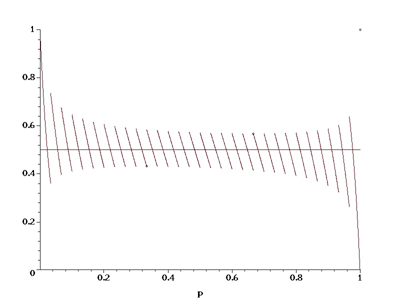
Figure 1. $\operatorname{\mathbb{P}{}}(\operatorname{Bi}(n,p)\leqslant np)$ for $n=30$. For integer values of $m=np$, the minimum of $\operatorname{\mathbb{P}{}}(\operatorname{Bi}(n,p)\leqslant np)$ (at $m=20$) and the maximum of $\operatorname{\mathbb{P}{}}(\operatorname{Bi}(n,p)<np)$ (at $m=10$) are marked with dots.

Consider again the case when $np=m$ is an integer, illustrated by the local maxima in Figure 1. Vašek Chvátal (personal communication) made the following conjecture, based on numerical experiments.

Conjecture 1.1 (Chvátal).

For any fixed $n\geqslant 2$, as $m$ ranges over $\{0,\dots,n\}$, the probability $q_{m}:=\operatorname{\mathbb{P}{}}\bigl{(}\operatorname{Bi}(n,m/n)\leqslant m\bigr{)}$ is smallest when $m$ is the integer closest to $2n/3$.

The purpose of the present paper is to show that this conjecture holds for large $n$. Moreover, at least for large $n$, the probabilities $q_{m}$ are inverse unimodal, i.e, have no other local minimum. (The latter property was partly proved by Rigollet and Tong [16, (29)], who proved, for any $n$, that $q_{m}$ decreases for $m\leqslant n/2$. We conjecture that also the inverse unimodality holds for all $n$.)

Theorem 1.2.

There exists $n_{0}$ such that Conjecture 1.1 is true for every $n\geqslant n_{0}$. Moreover, still for $n\geqslant n_{0}$, the difference $q_{m+1}-q_{m}$ is negative when $m+\frac{1}{2}<2n/3$ and positive when $m+\frac{1}{2}>2n/3$.

Remark 1.3.

By symmetry, i.e, considering $n-\operatorname{Bi}(n,m/n)$, it follows that for large $n$ at least, the probability $\operatorname{\mathbb{P}{}}(\operatorname{Bi}(n,m/n)<m)$ is largest for the integer $m$ closest to $n/3$. ∎

Remark 1.4.

For general $p$, the value of $\operatorname{\mathbb{P}{}}\bigl{(}\operatorname{Bi}(n,p)\leqslant np\bigr{)}$ is asymptotically given by

$$\operatorname{\mathbb{P}{}}\bigl{(}\operatorname{Bi}(n,p)\leqslant np\bigr{)}=\frac{1}{2}+\frac{4-2p-6\{np\}}{6\sqrt{2\pi np(1-p)}}+O\left(\frac{1}{np(1-p)}\right),$$ (1.2)

at least provided $np(1-p)\geqslant\log^{2}n$; this is a consequence of Theorem 3.2 and (5.1) (with $k=1$). Cf. Figure 1. See also the explicit related bound by Doerr [4, Lemma 8]. ∎

Remark 1.5.

In principle, it should be possible to calculate all constants in our proof explicitly, and thus find an explicit value for $n_{0}$; the conjecture then could be verified completely (assuming that it holds) by checking all smaller $n$ numerically. However, we do not believe that this is practical. Presumably, other methods, completely different from ours, are needed to show Chvátal’s conjecture in general. (We have verified the conjecture numerically for $n\leqslant 1000$.) ∎

Our proof of Theorem 1.2 is based on the version for integer-valued random variables found by Esseen [6] of the asymptotic Edgeworth expansion for probabilities in the central limit theorem. This is usually stated for a single probability distribution, but we need to check that the estimates hold uniformly for $\operatorname{Bi}(n,p)$ with $p$ in some range; hence we discuss this expansion in some detail in Section 3. In particular, we state in Theorem 3.2 the result that we need in a general form, and prove it in Section 4. We return to the binomial probabilities in Section 5, and prove Theorem 1.2 in Section 6.

Remark 1.6.

See Brown, Cai and DasGupta [3] for another aspect, with statistical implications, of the oscillations of binomial probabilities; they too use Edgeworth expansions with more than one term. ∎

2. Preliminaries

2.1. General notation

We let $\{x\}:=x-\lfloor x\rfloor$ denote the fractional part of a real number $x$; thus $\{x\}\in[0,1)$.

$f^{(m)}$ denotes the $m$th derivative of a function $f$, with $f^{(0)}:=f$.

A random variable $X$ has span $d$ if it is concentrated on a set $x_{0}+d\mathbb{Z}$ for some real $x_{0}$, and $d$ is maximal with this property.

$C$ and $c$ denote unimportant constants, in general different at different occurrences. The “constants” may depend on some given parameters, given by the context; we sometimes write e.g $C_{k}$ to emphasize that $C$ depends on a parameter $k$, but this is omitted when not necessary.

2.2. Special notation

We introduce here the notation needed for the expansions in the following sections. See further Esseen [6, Chapters III–IV] and Petrov [15, §VI.1].

Let $X$ be a random variable. ($X$ will be regarded as given. Most quantities defined below depend on the distribution of $X$, although we for simplicity do not show this in the notation.) Denote its mean by $\mu:=\operatorname{\mathbb{E}{}}X$, its central absolute moments by $\beta_{j}:=\operatorname{\mathbb{E}{}}|X-\mu|^{j}$, and its cumulants by $\gamma_{j}$ (when they exist, i.e, when $\operatorname{\mathbb{E}{}}|X|^{j}<\infty$). Also, let $\sigma^{2}=\beta_{2}=\gamma_{2}=\operatorname{Var}X$ be the variance of $X$, and define the scale-invariant

$$\Lambda_{j} :=\frac{\beta_{j}}{\sigma^{j}},$$ (2.1)

$$\lambda_{j} :=\frac{\gamma_{j}}{\sigma^{j}}.$$ (2.2)

Each cumulant $\gamma_{j}$, $j\geqslant 2$, can be expressed as a polynomial in central moments of orders $2,\dots,j$, and it follows, using also Hölder’s inequality, that

$$|\gamma_{j}|\leqslant C_{j}\beta_{j}$$ (2.3)

and thus

$$|\lambda_{j}|\leqslant C_{j}\Lambda_{j}.$$ (2.4)

Furthermore, Hölder’s inequality also easily yields, for $2\leqslant j\leqslant k$,

$$1=\Lambda_{2}\leqslant\Lambda_{j}^{1/(j-2)}\leqslant\Lambda_{k}^{1/(k-2)}.$$ (2.5)

Define polynomials $P_{j}(u)$, $j\geqslant 1$, by expanding the formal power series

$$\exp\left(\sum_{i=1}^{\infty}\frac{\lambda_{i+2}}{(i+2)!}u^{i+2}z^{i}\right)=1+\sum_{j=1}^{\infty}P_{j}(u)z^{j}.$$ (2.6)

Note that $P_{j}(u)$ is a polynomial of degree $3j$; moreover,

$$P_{j}(u)=\sum_{r=j+2}^{3j}\varpi_{jr}u^{r},$$ (2.7)

where each coefficient $\varpi_{jr}$ is a polynomial in $\lambda_{k}$, $k=3,\dots,j+2$. In particular, $P_{j}(u)$ is well-defined provided $\operatorname{\mathbb{E}{}}|X|^{j+2}<\infty$. Furthermore, $\varpi_{jr}=0$ unless $r-j$ is even.

Let $\Phi(x)$ be the distribution function of the standard normal distribution, so that

$$\frac{\mathrm{d}}{\mathrm{d}x}\Phi(x)=\phi(x):=\frac{1}{\sqrt{2\pi}}e^{-x^{2}/2}.$$ (2.8)

Define $Q_{j}(x)$ as the function obtained from $P_{j}(u)$ by replacing each power $u^{r}$ by $(-1)^{r}\Phi^{(r)}(x)=(-1)^{r}\frac{\mathrm{d}^{r}}{\mathrm{d}x^{r}}\Phi(x)$, i.e,

$$Q_{j}(x) :=\sum_{r=j+2}^{3j}(-1)^{r}\varpi_{jr}\Phi^{(r)}(x)=\sum_{r=j+2}^{3j}(-1)^{r}\varpi_{jr}\phi^{(r-1)}(x)$$ (2.9)

$$=-\phi(x)\sum_{r=j+2}^{3j}\varpi_{jr}H_{r-1}(x),$$ (2.10)

where $H_{r}(x)$ are the Hermite polynomials (in the normalization natural in probability theory, i.e, orthogonal w.r.t. the standard normal distruibution); see e.g [13, (18.5.9)] (there denoted $He_{r}(x)$) or [15, p. 127].

Define also periodic functions $\psi_{r}$, $r\geqslant 1$, by their Fourier series

$$\psi_{r}(x)=\sum_{\begin{subarray}{c}k=-\infty\\ k\neq 0\end{subarray}}^{\infty}\frac{e^{2\pi kx\mathrm{i}}}{(2\pi k\mathrm{i})^{r}}.$$ (2.11)

Note that for $r\geqslant 2$, the series (2.11) converges absolutely and defines a continuous periodic function with period 1. However, for $r=1$, the series is only conditionally convergent; in fact it is the Fourier series of $\frac{1}{2}-\{x\}$. (It follows from standard results that the series converges for every $x$, but we do not really need this.) Hence, $\psi_{1}(x)$ has a jump 1 at every integer. For later convenience, we redefine $\psi_{1}$ to be right-continuous; thus we define

$$\psi_{1}(x):=\frac{1}{2}-\{x\}=\frac{1}{2}-x+\lfloor x\rfloor,\qquad x\in\mathbb{R},$$ (2.12)

noting that for $r=1$, (2.11) holds only for non-integer $x$. Note also that, for any $r\geqslant 1$ and $x\in\mathbb{R}$,

$$\psi_{r}(x)=-\frac{1}{r!}B_{r}(\{x\}),$$ (2.13)

where $B_{r}(x)$ denotes the Bernoulli polynomials, see e.g [13, (24.8.3)]. In particular, [13, (24.2.4)],

$$\psi_{r}(0)=-\frac{1}{r!}B_{r}(0)=-\frac{1}{r!}B_{r},$$ (2.14)

where $B_{r}$ denotes the Bernoulli numbers. Recall that $B_{1}=-\frac{1}{2}$, $B_{2}=\frac{1}{6}$ and $B_{2j+1}=0$ for $j\geqslant 1$.

Remark 2.1.

Note that $\psi_{r}(x)=(-1)^{r-1}h_{r}Q_{r}(x)$ (where $h_{r}=\pm 1$) in the notation of [6, p. 60–61]. We prefer the choice of signs in our definition, but this is only a matter of taste. ∎

3. The basic expansion theorem

Esseen [6, Theorem IV.4] proved the following. More precisely, Esseen’s result is (3.4); the version (3.5) follows immediately by applying (3.4) with $k+1$ instead of $k$. (We prefer this, weaker, version for our generalization in Theorem 3.2.)

Theorem 3.1 (Esseen [6]).

Let $X,X_{1},X_{2},\dots$ be i.i.d integer valued random variables with span $1$ and let $S_{n}:=\sum_{i=1}^{n}X_{i}$. Let $k\geqslant 1$ be an integer and suppose that $\operatorname{\mathbb{E}{}}|X|^{k+2}<\infty$. With notations as above, define

$$\Psi_{n,k}(x):=\Phi(x)+\sum_{j=1}^{k}n^{-j/2}Q_{j}(x)$$ (3.1)

and

$$\Psi^{*}_{n,k}(x):=\Psi_{n,k}(x)+\sum_{\ell=1}^{k}(-1)^{\ell-1}n^{-\ell/2}\sigma^{-\ell}\psi_{\ell}\bigl{(}n\mu+x\sigma\sqrt{n}\bigr{)}\Psi_{n,k}^{(\ell)}(x).$$ (3.2)

Then

$$\operatorname{\mathbb{P}{}}\bigl{(}S_{n}\leqslant n\mu+x\sigma\sqrt{n}\bigr{)}=\Psi^{*}_{n,k}(x)+R_{n,k}(x),$$ (3.3)

where, as ${n\to\infty}$,

$$\sup_{x}|R_{n,k}(x)|=o\bigl{(}n^{-k/2}\bigr{)}.$$ (3.4)

If further $\operatorname{\mathbb{E}{}}|X|^{k+3}<\infty$, then

$$\sup_{x}|R_{n,k}(x)|=O\bigl{(}n^{-\frac{k+1}{2}}\bigr{)}.$$ (3.5)

Theorem 3.1 is stated for a single distribution. We want to apply it to $X\sim\operatorname{Be}(p)$, but then need some uniform estimates for all $p$, or at least for a large range. It is no surprise that the proof of Theorem 3.1 yields such uniformity under suitable conditions, including some uniform moment estimates. For $\operatorname{Be}(p)$, the case $p\in[p_{1},p_{2}]$ for a compact interval $[p_{1},p_{2}]\subset(0,1)$ does not cause any difficulties, but we can go beyond that. We will show the following extension of Theorem 3.1 in Section 4.

Theorem 3.2.

Let $k\geqslant 1$. For every $c>0$, there exists a constant $C$ (depending on $k$ and $c$ only) such that if $X$ is an integer-valued random variable with $\operatorname{\mathbb{E}{}}|X|^{k+3}<\infty$ and

$$\min\bigl{\{}\operatorname{\mathbb{P}{}}(X=0),\operatorname{\mathbb{P}{}}(X=1)\bigr{\}} \geqslant c\sigma^{2},$$ (3.6)

and $n\geqslant 2$ is an integer with

$$\sigma\sqrt{n}\geqslant\log n,$$ (3.7)

then (3.3) holds with

$$\sup_{x}|R_{n,k}(x)|\leqslant C\Lambda_{k+3}n^{-\frac{k+1}{2}}\leqslant C\frac{\operatorname{\mathbb{E}{}}|X|^{k+3}}{\sigma^{k+3}}n^{-\frac{k+1}{2}}.$$ (3.8)

Remark 3.3.

We defined $\psi_{1}(x)$ to be right-continuous so that $\Psi^{*}_{n,k}(x)$ and $R_{n,k}(x)$ are right-continuous, which enables (3.4), (3.5) and (3.8) to hold for all $x$, including integers. (All functions in (3.1)–(3.2) except $\psi_{1}$ are continuous.) ∎

Remark 3.4.

As remarked by Esseen [6, p. 61], (3.2) contains redundant terms. The form (3.2) is sometimes convenient (for example in the proof), but it is often more convenient to modify (3.2) by dropping the redundant terms; we thus define also

$$\widetilde{\Psi}^{*}_{n,k}(x):=\Psi_{n,k}(x)+\sum_{\ell=1}^{k}(-1)^{\ell-1}n^{-\ell/2}\sigma^{-\ell}\psi_{\ell}\bigl{(}n\mu+x\sigma\sqrt{n}\bigr{)}\Psi_{n,k-\ell}^{(\ell)}(x)$$ (3.9)

and define a modified remainder term $\widetilde{R}_{n,k}(x)$ by

$$\operatorname{\mathbb{P}{}}\bigl{(}S_{n}\leqslant n\mu+x\sigma\sqrt{n}\bigr{)}=\widetilde{\Psi}^{*}_{n,k}(x)+\widetilde{R}_{n,k}(x).$$ (3.10)

It follows from (3.1) that in Theorem 3.1, this changes $\Psi^{*}_{n,k}(x)$ and thus $R_{n,k}(x)$ by some terms which are $O(n^{-m/2})$ for some $m\geqslant k+1$ so (3.4) and (3.5) still hold for $\widetilde{R}_{n,k}(x)$. With only a little more effort, it can be verified that the same holds for Theorem 3.2; it follows from Lemma 4.1 below that the removed terms are all dominated by $\Lambda_{k+3}n^{-\frac{k+1}{2}}$, so (3.8) still holds. (This uses also that $\sigma\sqrt{n}$ is bounded below by the assumptions, and the fact that $\beta_{i}\leqslant C_{i,j}\beta_{j}$ when $2\leqslant i\leqslant j$ and $X$ is integer valued.) ∎

Remark 3.5.

Note that Theorem 1.2 is only for random variables with span 1, and that a uniform version for a family of random variables therefore requires some uniform condition preventing the variables from being too close to variables with larger span. We use condition (3.6) which is convenient and turns out to be sufficient; it can obviously be replaced by more general conditions. ∎

Remark 3.6.

The assumption (3.7) in Theorem 3.2 is annoying but not a very serious restriction. Note that the right-hand side of (3.8) is, since $X$ is integer-valued, at least $C(\sigma\sqrt{n})^{-k-1}$. Hence, if (3.7) is violated, (3.8) would, even if true, only give a weak bound. We do not know whether (3.7) really is needed. It is possible that Theorem 3.2 could be proved without this assumption, using the alternative method of proof in [6, Section IV.4], but we have not pursued this. ∎

4. Proof of Theorem 3.2

Lemma 4.1.

Suppose that $\ell\geqslant 1$ and $\operatorname{\mathbb{E}{}}|X|^{\ell+2}<\infty$. Then, for every $m\geqslant 0$,

$$|\varpi_{\ell,r}| \leqslant C_{\ell}\Lambda_{\ell+2},$$ (4.1)

$$|P_{\ell}(u)| \leqslant C_{\ell}\Lambda_{\ell+2}\bigl{(}|u|^{\ell+2}+|u|^{3\ell}\bigr{)},$$ (4.2)

$$|Q_{\ell}^{(m)}(x)| \leqslant C_{\ell,m}\Lambda_{\ell+2},$$ (4.3)

$$|\Psi_{n,\ell}^{(m)}(x)| \leqslant C_{\ell,m}\bigl{(}1+\Lambda_{\ell+2}n^{-\ell/2}\bigr{)}.$$ (4.4)

Proof.

It follows from (2.6) that $\varpi_{\ell,r}$ is a linear combination of products $\prod_{k=1}^{m}\lambda_{i_{k}+2}$ with $\sum_{k}(i_{k}+2)=r$ and $\sum_{k}i_{k}=\ell$. By (2.4) and (2.5), each such product is bounded by

$$C_{\ell}\prod_{k=1}^{m}\Lambda_{i_{k}+2}\leqslant C_{\ell}\prod_{k=1}^{m}\Lambda_{\ell+2}^{i_{k}/\ell}=C_{\ell}\Lambda_{\ell+2},$$ (4.5)

which yields (4.1). This implies (4.2) and (4.3) by (2.7) and (2.9), noting that $\Phi(x)$ and all its derivatives are bounded on $\mathbb{R}$. Finally, (3.1) and (4.3) together with (2.5) yield

$$|\Psi_{n,\ell}^{(m)}(x)| \leqslant C_{m}+C_{\ell,m}\sum_{j=1}^{\ell}n^{-j/2}\Lambda_{j+2}\leqslant C_{\ell,m}\sum_{j=0}^{\ell}n^{-j/2}\Lambda_{\ell+2}^{j/\ell}$$

$$\leqslant C_{\ell,m}\bigl{(}1+n^{-\ell/2}\Lambda_{\ell+2}\bigr{)}.$$ (4.6)

∎

Lemma 4.2.

If $X$ is a random variable with $\operatorname{\mathbb{P}{}}(X=0)\geqslant a$ and $\operatorname{\mathbb{P}{}}(X=1)\geqslant a$ for some $a\geqslant 0$, then

$$\bigl{\lvert}\operatorname{\mathbb{E}{}}e^{\mathrm{i}tX}\bigr{\rvert}\leqslant 1-\frac{a}{\pi^{2}}t^{2}\leqslant e^{-a\pi^{-2}t^{2}},\qquad|t|\leqslant\pi.$$ (4.7)

Proof.

The assumption implies that $\operatorname{\mathbb{E}{}}e^{\mathrm{i}tX}-a-ae^{\mathrm{i}t}$ is the Fourier transform of a positive measure with mass $1-2a$. Hence, if $|t|\leqslant\pi$,

$$\bigl{\lvert}\operatorname{\mathbb{E}{}}e^{\mathrm{i}tX}\bigr{\rvert} \leqslant\bigl{\lvert}a+ae^{\mathrm{i}t}\bigr{\rvert}+\bigl{\lvert}\operatorname{\mathbb{E}{}}e^{\mathrm{i}tX}-a-ae^{\mathrm{i}t}\bigr{\rvert}\leqslant a\bigl{\lvert}1+e^{\mathrm{i}t}\bigr{\rvert}+1-2a$$

$$=2a\bigl{\lvert}\cos\frac{t}{2}\bigr{\rvert}+1-2a=1-2a\bigl{(}1-\cos\frac{t}{2}\bigr{)}=1-4a\sin^{2}\frac{t}{4},$$ (4.8)

and (4.7) follows. ∎

Proof of Theorem 3.2.

We follow the proofs of Theorems 3 and 4 in Esseen [6] (with $d=1$ and thus $t_{0}=2\pi$) and mention only the main differences. Note that [6] considers centred variables, so $X_{i}$ there is our $X_{i}-\mu$. Let

$$f(t) :=\operatorname{\mathbb{E}{}}e^{\mathrm{i}t(X-\mu)},$$ (4.9)

$$f_{n}(t) :=\operatorname{\mathbb{E}{}}e^{\mathrm{i}t(S_{n}-n\mu)/(\sigma\sqrt{n})}=f^{n}\bigl{(}t/(\sigma\sqrt{n})\bigr{)},$$ (4.10)

$$g_{0}(t) :=e^{-t^{2}/2}+\sum_{j=1}^{k}n^{-j/2}P_{j}(\mathrm{i}t)e^{-t^{2}/2}.$$ (4.11)

Also, let $T:=n^{\frac{k+1}{2}}$ and replace $T_{3n}$ in [6] by

$$T_{1}:=\sqrt{n}/\Lambda_{k+3}^{1/(k+1)}.$$ (4.12)

The second inequality in (3.8) is trivial, by the definition (2.1). We may also assume that $\Lambda_{k+3}n^{-\frac{k+1}{2}}\leqslant 1$, and thus $T_{1}\geqslant 1$, since otherwise it follows from Lemma 4.1 and (2.5) that each term in (3.2) is bounded by $C\Lambda_{k+3}n^{-\frac{k+1}{2}}$, and thus (3.8) holds trivially.

In the range $|t|\leqslant T_{1}$, we have

$$|f_{n}(t)-g_{0}(t)|\leqslant C\Lambda_{k+3}|t|^{k+3}e^{-t^{2}/13}n^{-\frac{k+1}{2}}$$ (4.13)

by [15, Lemma VI.4] with $s=k+3$ and $m=0$ (which essentially is [6, Lemma IV.2a] with $T_{3n}$ improved to our $T_{1}/4$, which can be proved in the same way). Hence, for the “main term” in the estimate

$$\int_{-T_{1}}^{T_{1}}\frac{|f_{n}(t)-g_{0}(t)|}{|t|}\,\mathrm{d}t\leqslant C\Lambda_{k+3}n^{-\frac{k+1}{2}}.$$ (4.14)

Furthermore, if $|t|\leqslant\pi\sigma\sqrt{n}$, then the assumption (3.6) and Lemma 4.2 yield

$$|f_{n}(t)|=\bigl{\lvert}f\bigl{(}t/(\sigma\sqrt{n})\bigr{)}\bigr{\rvert}^{n}\leqslant e^{-nc\sigma^{2}(t/\sigma\sqrt{n})^{2}}=e^{-ct^{2}}.$$ (4.15)

Hence,

$$\int_{T_{1}}^{\pi\sigma\sqrt{n}}\frac{|f_{n}(t)|}{|t|}\,\mathrm{d}t\leqslant\int_{T_{1}}^{\pi\sigma\sqrt{n}}{|f_{n}(t)|}\,\mathrm{d}t\leqslant Ce^{-cT_{1}^{2}}\leqslant CT_{1}^{-(k+1)}=C\Lambda_{k+3}n^{-\frac{k+1}{2}}.$$ (4.16)

The integral $\int_{T_{1}}^{\pi\sigma\sqrt{n}}|g_{0}(t)|/|t|\,\mathrm{d}t$ has the same estimate. Consequently, by (4.14) and (4.16),

$$\int_{-\pi\sigma\sqrt{n}}^{\pi\sigma\sqrt{n}}\frac{|f_{n}(t)-g_{0}(t)|}{|t|}\,\mathrm{d}t\leqslant C\Lambda_{k+3}n^{-\frac{k+1}{2}}.$$ (4.17)

The same arguments yield also

$$\int_{-\pi\sigma\sqrt{n}}^{\pi\sigma\sqrt{n}}|f_{n}(t)-g_{0}(t)|\,\mathrm{d}t\leqslant C\Lambda_{k+3}n^{-\frac{k+1}{2}}.$$ (4.18)

Using the estimates (4.17) and (4.18), the rest of the proof is essentially the same as in [6]. One of the terms, generalizing $I^{\prime}_{k}$ on [6, p. 58–59], is

$$\int_{-\pi\sigma\sqrt{n}}^{\pi\sigma\sqrt{n}}\frac{|f_{n}(t)-g_{0}(t)|}{|t+2\pi j\sigma\sqrt{n}|}\,\mathrm{d}t\leqslant\frac{C}{|j|\sigma\sqrt{n}}\Lambda_{k+3}n^{-\frac{k+1}{2}},$$ (4.19)

where we use (4.18). This term exists for all integers $j\neq 0$ with $(2|j|-1)\pi\sigma\sqrt{n}<T=n^{\frac{k+1}{2}}$, and thus the sum of them is bounded by

$$2\sum_{j=1}^{T}\frac{C}{|j|\sigma\sqrt{n}}\Lambda_{k+3}n^{-\frac{k+1}{2}}\leqslant C\frac{\log n}{\sigma\sqrt{n}}\Lambda_{k+3}n^{-\frac{k+1}{2}};$$ (4.20)

this is the reason for our assumption $\log n\leqslant\sigma\sqrt{n}$, which leads to an estimate $C\Lambda_{k+3}n^{-\frac{k+1}{2}}$ for (4.19) too. The remaining terms give no problems. ∎

5. Expansions for the binomial probabilities

Taking $x=0$ in (3.9)–(3.10), we obtain

$$\operatorname{\mathbb{P}{}}(S_{n}\leqslant n\mu)=\Psi_{n,k}(0)+\sum_{\ell=1}^{k}(-1)^{\ell-1}n^{-\ell/2}\sigma^{-\ell}\psi_{\ell}(n\mu)\Psi_{n,k-\ell}^{(\ell)}(0)+\widetilde{R}_{n,k}(0).$$ (5.1)

If furthermore $n\mu$ is an integer, this yields, using (2.14) and $B_{0}:=1$, and for convenience defining $Q_{0}(x):=\Phi(x)$,

$$\operatorname{\mathbb{P}{}}(S_{n}\leqslant n\mu) =\Psi_{n,k}(0)+\sum_{\ell=1}^{k}(-1)^{\ell-1}n^{-\ell/2}\sigma^{-\ell}\psi_{\ell}(0)\Psi_{n,k-\ell}^{(\ell)}(0)+\widetilde{R}_{n,k}(0)$$

$$=\sum_{\ell=0}^{k}\sum_{j=0}^{k-\ell}n^{-(j+\ell)/2}\sigma^{-\ell}\frac{(-1)^{\ell}B_{\ell}}{\ell!}Q_{j}^{(\ell)}(0)+\widetilde{R}_{n,k}(0)$$

$$=\frac{1}{2}+\sum_{m=1}^{k}n^{-m/2}\sum_{\ell=0}^{m}\sigma^{-\ell}\frac{(-1)^{\ell}B_{\ell}}{\ell!}Q_{m-\ell}^{(\ell)}(0)+\widetilde{R}_{n,k}(0).$$ (5.2)

Since $\phi(x)$ is an even function, all its odd derivatives vanish at 0, and since $\varpi_{jr}=0$ unless $j\equiv r\pmod{2}$, it follows from (2.9) that $Q^{(\ell)}_{j}(0)=0$ when $j\equiv\ell\pmod{2}$ (except when $j=\ell=0$). Hence, all terms in (5) with $m$ even vanish.

Remark 5.1.

For $\operatorname{\mathbb{P}{}}(S_{n}<n\mu)$, we have the same formulas with $\psi_{1}(x)$ replaced by its left-continuous version $\psi_{1}(x-)$. (All other appearing functions are continuous.) In (5), this means that the sign is changed for the terms with $\ell=1$; all other terms remain the same. ∎

We specialize to $X\sim\operatorname{Be}(p)$, with $0<p<1$, so $S_{n}\sim\operatorname{Bi}(n,p)$. All moments exist, and we have $\sigma^{2}:=p(1-p)$. Furthermore, $\beta_{j}:=\operatorname{\mathbb{E}{}}|X-p|^{j}\leqslant\beta_{2}=\sigma^{2}$; hence, recalling (2.1) and (2.4),

$$|\lambda_{j}|\leqslant C_{j}\Lambda_{j}\leqslant C_{j}\sigma^{2-j}.$$ (5.3)

The condition (3.6) holds with $c=1$ for all $p$. Hence Theorem 3.2 applies provided

$$\sqrt{np(1-p)}\geqslant\log n,$$ (5.4)

and then yields, together with Remark 3.4 and using (5.3),

$$|R_{n,k}(x)|,|\widetilde{R}_{n,k}(x)|\leqslant C_{k}\Lambda_{k+3}n^{-\frac{k+1}{2}}\leqslant\frac{C_{k}}{(n\sigma^{2})^{(k+1)/2}}=\frac{C_{k}}{(np(1-p))^{(k+1)/2}}$$ (5.5)

We use (5) with $k=4$ and obtain, when $np$ is an integer,

$$\operatorname{\mathbb{P}{}}(S_{n}\leqslant np)=\frac{1}{2}+h_{1}(p)n^{-1/2}+h_{3}(p)n^{-3/2}+O\bigl{(}(np(1-p))^{-5/2}\bigr{)},$$ (5.6)

where, after some calculations using (2.10) and (2.6) after finding the cumulants $\gamma_{3},\gamma_{4},\gamma_{5}$,

$$h_{1}(p) :=Q_{1}(0)+\frac{1}{2\sigma}Q_{0}^{\prime}(0)=\frac{\gamma_{3}}{6\sqrt{2\pi}\sigma^{3}}+\frac{1}{2\sqrt{2\pi}\sigma}=\frac{2-p}{3\sqrt{2\pi}\sqrt{p(1-p)}},$$ (5.7)

$$h_{3}(p) :=Q_{3}(0)+\frac{1}{2\sigma}Q_{2}^{\prime}(0)+\frac{1}{12\sigma^{2}}Q_{1}^{\prime\prime}(0)=\frac{(2-p)(p^{2}+23p-23)}{540\sqrt{2\pi}(p(1-p))^{3/2}}.$$ (5.8)

Recall that there is no $h_{2}(p)$ or $h_{4}(p)$; the corresponding terms vanish as said above.

6. Proof of Theorem 1.2

We now prove our main result.

Proof of Theorem 1.2.

The main idea of the proof is to estimate $q_{m+1}-q_{m}$ using the estimates above, in particular (5.6), but the details will differ for different ranges of $m$. We write $p_{m}:=m/n$. We sometimes tacitly assume that $n$ is large enough. $C_{1},C_{2},C_{3}$ will denote some large constants.

Recall $h_{1}(p)$ and $h_{3}(p)$ given in (5.7)–(5.8). A simple differentiation yields

$$h_{1}^{\prime}(p)=\frac{3p-2}{6\sqrt{2\pi}(p(1-p))^{3/2}}.$$ (6.1)

Note that $h_{1}^{\prime}(p)=0$ for $p=2/3$, with $h^{\prime}(p)<0$ for $0<p<2/3$ and $h^{\prime}(p)>0$ for $2/3<p<1$; this is the fundamental reason for the behaviour shown in Theorem 1.2, although we also have to treat error terms.

There is no need to calculate $h_{3}^{\prime}(p)$ exactly; it suffices to note from (5.8) that

$$h_{3}^{\prime}(p)=O\bigl{(}(p(1-p))^{-5/2}\bigr{)}.$$ (6.2)

We treat several cases separately.

Case 1: $2\log^{2}n\leqslant m\leqslant n-2\log^{2}n$. Both $p_{m}$ and $p_{m+1}$ satisfy (5.4); hence Theorem 3.2 applies and yields (5.6) for both. By subtraction and the mean value theorem, we obtain, for some $p_{m}^{\prime},p_{m}^{\prime\prime}\in[p_{m},p_{m+1}]$, recalling that $p_{m+1}-p_{m}=n^{-1}$ and using (6.1)–(6.2),

$$q_{m+1}-q_{m} =h_{1}^{\prime}(p_{m}^{\prime})n^{-3/2}+h_{3}^{\prime}(p_{m}^{\prime\prime})n^{-5/2}+O\bigl{(}(np_{m})^{-5/2}\bigr{)}$$ (6.3)

$$=\frac{3p_{m}-2+O(1/n)}{6\sqrt{2\pi}}(np_{m}^{\prime}(1-p_{m}^{\prime}))^{-3/2}+O\bigl{(}(np_{m})^{-5/2}\bigr{)}.$$ (6.4)

Case 1a: $2\log^{2}n\leqslant m\leqslant n/2$. In this subcase, (6.4) yields

$$q_{m+1}-q_{m} \leqslant-c(np_{m})^{-3/2}+O\bigl{(}(np_{m})^{-5/2}\bigr{)}<0,$$ (6.5)

provided $n$ and thus $np_{m}=m$ is large enough.

Case 1b: $n/2\leqslant m\leqslant 2n/3-C_{1}$. In this subcase, (6.4) similarly yields

$$q_{m+1}-q_{m} \leqslant-\frac{3C_{1}}{6\sqrt{2\pi}}cn^{-5/2}+O\bigl{(}n^{-5/2}\bigr{)}<0,$$ (6.6)

provided $C_{1}$ is chosen large enough.

Case 1c: $2n/3+C_{2}\leqslant m\leqslant n-2\log^{2}n$. Similar arguments as in the two preceding subcases yield $q_{m+1}-q_{m}>0$.

Case 1d: $2n/3-C_{1}\leqslant m\leqslant 2n/3+C_{2}$. This is the most delicate case, since $p_{m}-2/3=O(1/n)$ and the three terms in (6.3) all are of the same order. We thus expand one step further and use Theorem 3.2 with $k=6$; this yields, again using (5),

$$q_{m}=\frac{1}{2}+h_{1}(p_{m})n^{-1/2}+h_{3}(p_{m})n^{-3/2}+h_{5}(p_{m})n^{-5/2}+O\bigl{(}n^{-7/2}\bigr{)},$$ (6.7)

where we note that $h_{5}(p)$ is a differentiable function of $p$. (It can easily be calculated, but we do not need this.) Taylor expansions yield, recalling $h_{1}^{\prime}(\tfrac{2}{3})=0$,

$$q_{m} =\frac{1}{2}+h_{1}\bigl{(}\tfrac{2}{3}\bigr{)}n^{-1/2}+\frac{1}{2}h_{1}^{\prime\prime}\bigl{(}\tfrac{2}{3}\bigr{)}\bigl{(}p_{m}-\tfrac{2}{3}\bigr{)}^{2}n^{-1/2}+h_{3}\bigl{(}\tfrac{2}{3}\bigr{)}n^{-3/2}$$

$$\qquad+h_{3}^{\prime}\bigl{(}\tfrac{2}{3}\bigr{)}\bigl{(}p_{m}-\tfrac{2}{3}\bigr{)}n^{-3/2}+h_{5}\bigl{(}\tfrac{2}{3}\bigr{)}n^{-5/2}+O\bigl{(}n^{-7/2}\bigr{)}$$

$$=G(n)+H\bigl{(}m-2n/3\bigr{)}n^{-5/2}+O\bigl{(}n^{-7/2}\bigr{)},$$ (6.8)

where we define

$$G(n) :=\frac{1}{2}+h_{1}\bigl{(}\tfrac{2}{3}\bigr{)}n^{-1/2}+h_{3}\bigl{(}\tfrac{2}{3}\bigr{)}n^{-3/2}+h_{5}\bigl{(}\tfrac{2}{3}\bigr{)}n^{-5/2},$$ (6.9)

$$H(x) :=\frac{1}{2}h_{1}^{\prime\prime}\bigl{(}\tfrac{2}{3}\bigr{)}x^{2}+h_{3}^{\prime}\bigl{(}\tfrac{2}{3}\bigr{)}x.$$ (6.10)

The formula (6) holds for $m+1$ too, and thus

$$q_{m+1}-q_{m} =\bigl{(}H(m+1-2n/3)-H(m-2n/3)\bigr{)}n^{-5/2}+O\bigl{(}n^{-7/2}\bigr{)}$$

$$=\Bigl{(}h_{1}^{\prime\prime}\bigl{(}\tfrac{2}{3}\bigr{)}\bigl{(}m-\frac{2n}{3}+\frac{1}{2}\bigr{)}+h_{3}^{\prime}\bigl{(}\tfrac{2}{3}\bigr{)}\Bigr{)}n^{-5/2}+O\bigl{(}n^{-7/2}\bigr{)}$$ (6.11)

A calculation yields

$$h_{1}^{\prime\prime}(2/3) =\frac{27}{8\sqrt{\pi}},$$ (6.12)

$$h_{3}^{\prime}(2/3) =\frac{9}{40\sqrt{\pi}}=\frac{1}{15}h_{1}^{\prime\prime}(2/3).$$ (6.13)

Since the ratio $1/15<1/6$, it follows from (6) that if $m\leqslant(2n-2)/3$, then $q_{m+1}-q_{m}<0$, and if $m\geqslant(2n-1)/3$, then $q_{m+1}-q_{m}>0$, for large $n$.

Case 2: $m<2\log^{2}n$. As said in the introduction, Rigollet and Tong [16, (29)] showed that (for every $n$) $q_{m-1}\geqslant q_{m}$, and their proof actually gives $q_{m-1}>q_{m}$, for $m\leqslant n/2$. Alternatively (for large $n$), we can argue using Poisson approximation as in the next case; we omit the details.

Case 3: $m>n-2\log^{2}n$. Define $q_{m}^{\prime}:=\operatorname{\mathbb{P}{}}\bigl{(}\operatorname{Bi}(n,m/n)<m\bigr{)}$. By symmetry, $1-q_{m}=q^{\prime}_{n-m}$; hence the claim $q_{m}<q_{m+1}$ is equivalent to $q^{\prime}_{m-1}<q^{\prime}_{m}$ for $m<2\log^{2}n$.

We use Poisson approximation of the binomial distribution. It is well-known, see e.g [1, Theorem 2.M] that the total variation distance between $\operatorname{Bi}(n,p)$ and $\operatorname{Po}(np)$ is less than $p$, and thus, in particular,

$$\bigl{\lvert}q^{\prime}_{m}-\operatorname{\mathbb{P}{}}\bigl{(}\operatorname{Po}(m)<m\bigr{)}\bigr{\rvert}\leqslant d_{\mathrm{TV}}\bigl{(}\operatorname{Bi}(n,p_{m}),\operatorname{Po}(np_{m})\bigr{)}<p_{m}.$$ (6.14)

We estimate $\operatorname{\mathbb{P}{}}\bigl{(}\operatorname{Po}(m)<m\bigr{)}$ by Theorem 3.2 (or Theorem 3.1) applied to $X\sim\operatorname{Po}(1)$. This yields, using (5) and Remark 5.1,

$$\operatorname{\mathbb{P}{}}\bigl{(}\operatorname{Po}(m)<m\bigr{)}=\frac{1}{2}-\frac{1}{3\sqrt{2\pi}}m^{-1/2}-\frac{23}{270\sqrt{2\pi}}m^{-3/2}+O\bigl{(}m^{-5/2}\bigr{)}.$$ (6.15)

Combining (6.14) and (6.15) we find, for $m\geqslant 2$,

$$q_{m}^{\prime}-q^{\prime}_{m-1}=\frac{1}{6\sqrt{2\pi}}m^{-3/2}+O\bigl{(}m^{-5/2}\bigr{)}+O(m/n).$$ (6.16)

This shows that $q^{\prime}_{m}>q^{\prime}_{m-1}$ for $C_{3}<m<2\log^{2}n$ and $n$ large. (In fact, for $C_{3}<m<cn^{2/5}$.)

In the remaining subcase $m\leqslant C_{3}$, $q_{m-1}^{\prime}<q^{\prime}_{m}$ follows from (6.14) and Lemma 6.1 below.

These cases cover all $m$, which completes the proof of Theorem 1.2. ∎

The proof used the following lemma, of independent interest. It gives two Poisson versions of the inequality mentioned above for the binomial distribution shown by Rigollet and Tong [16]. We use their method of proof.

Lemma 6.1.

For every integer $m\geqslant 0$,

$$\operatorname{\mathbb{P}{}}\bigl{(}\operatorname{Po}(m)<m\bigr{)} <\operatorname{\mathbb{P}{}}\bigl{(}\operatorname{Po}(m+1)<m+1\bigr{)}<\frac{1}{2},$$ (6.17)

$$\operatorname{\mathbb{P}{}}\bigl{(}\operatorname{Po}(m)\leqslant m\bigr{)} >\operatorname{\mathbb{P}{}}\bigl{(}\operatorname{Po}(m+1)\leqslant m+1\bigr{)}>\frac{1}{2}.$$ (6.18)

Proof.

We may assume $m\geqslant 1$. Consider a Poisson process with intensity 1 on $(0,\infty)$ and denote its points by $T_{1}<T_{2}<\dots$. The number of points in $[0,m]$ is $\operatorname{Po}(m)$, and thus $\operatorname{Po}(m)<m\iff T_{m}>m$. The distribution of $T_{m}$ is $\Gamma(m)$, and thus

$$\operatorname{\mathbb{P}{}}\bigl{(}\operatorname{Po}(m)<m\bigr{)}=\operatorname{\mathbb{P}{}}(T_{m}>m)=\int_{m}^{\infty}\frac{t^{m-1}}{(m-1)!}e^{-t}\,\mathrm{d}t.$$ (6.19)

Hence,

$$\hskip-20.00003pt\operatorname{\mathbb{P}{}}\bigl{(}\operatorname{Po}(m)<m\bigr{)}-\operatorname{\mathbb{P}{}}\bigl{(}\operatorname{Po}(m+1)<m+1\bigr{)}$$

$$=\int_{m}^{\infty}\frac{t^{m-1}}{(m-1)!}e^{-t}\,\mathrm{d}t-\int_{m+1}^{\infty}\frac{t^{m}}{m!}e^{-t}\,\mathrm{d}t$$

$$=\int_{m}^{\infty}\left(\frac{t^{m-1}}{(m-1)!}e^{-t}-\frac{t^{m}}{m!}e^{-t}\right)\,\mathrm{d}t+\int_{m}^{m+1}\frac{t^{m}}{m!}e^{-t}\,\mathrm{d}t$$

$$=\Bigl{[}\frac{t^{m}}{m!}e^{-t}\Bigr{]}_{m}^{\infty}+\int_{m}^{m+1}\frac{t^{m}}{m!}e^{-t}\,\mathrm{d}t=\int_{m}^{m+1}\frac{t^{m}e^{-t}-m^{m}e^{-m}}{m!}\,\mathrm{d}t<0,$$ (6.20)

since $t^{m}e^{-t}$ is decreasing for $t\geqslant m$. Similarly,

$$\hskip-20.00003pt\operatorname{\mathbb{P}{}}\bigl{(}\operatorname{Po}(m)\leqslant m\bigr{)}-\operatorname{\mathbb{P}{}}\bigl{(}\operatorname{Po}(m+1)\leqslant m+1\bigr{)}$$

$$=\int_{m}^{\infty}\frac{t^{m}}{m!}e^{-t}\,\mathrm{d}t-\int_{m+1}^{\infty}\frac{t^{m+1}}{(m+1)!}e^{-t}\,\mathrm{d}t$$

$$=\int_{m}^{\infty}\left(\frac{t^{m}}{m!}e^{-t}-\frac{t^{m+1}}{(m+1)!}e^{-t}\right)\,\mathrm{d}t+\int_{m}^{m+1}\frac{t^{m+1}}{(m+1)!}e^{-t}\,\mathrm{d}t$$

$$=\int_{m}^{m+1}\frac{t^{m+1}e^{-t}-m^{m+1}e^{-m}}{(m+1)!}\,\mathrm{d}t>0,$$ (6.21)

since $t^{m+1}e^{-t}$ is increasing for $t\leqslant m+1$. ∎

References

- Barbour, Holst and Janson [1992] A. D. Barbour, Lars Holst & Svante Janson: Poisson Approximation. Oxford University Press, Oxford, 1992. MR 1163825
- [2] Andrew C. Berry: The accuracy of the Gaussian approximation to the sum of independent variates. Trans. Amer. Math. Soc. 49 (1941), 122–136. MR 0003498
- Brown, Cai and DasGupta [2002] Lawrence D. Brown, T. Tony Cai & Anirban DasGupta: Confidence intervals for a binomial proportion and asymptotic expansions. Ann. Statist. 30 (2002), no. 1, 160–201. MR 1892660
- Doerr [2018] Benjamin Doerr: An elementary analysis of the probability that a binomial random variable exceeds its expectation. Statist. Probab. Lett. 139 (2018), 67–74. MR 3802185
- Esseen [1942] Carl-Gustav Esseen: On the Liapounoff limit of error in the theory of probability. Ark. Mat. Astr. Fys. 28A (1942), no. 9, 19 pp. MR 0011909
- Esseen [1945] Carl-Gustav Esseen: Fourier analysis of distribution functions. A mathematical study of the Laplace–Gaussian law. Acta Math. 77 (1945), 1–125. MR 0014626
- [7] Spencer Greenberg & Mehryar Mohri: Tight lower bound on the probability of a binomial exceeding its expectation. Statist. Probab. Lett. 86 (2014), 91–98. MR 3162723
- [8] Allan Gut: Probability: A Graduate Course, 2nd ed., Springer, New York, 2013. MR 2977961
- [9] Kumar Jogdeo & S. M. Samuels: Monotone Convergence of Binomial Probabilities and a Generalization of Ramanujan’s Equation. Ann. Math. Statist. 39 (1968), 1191–1195.
- Kaas and Buhrman [1980] R. Kaas & J. M. Buhrman: Mean, median and mode in binomial distributions. Statist. Neerlandica 34 (1980), no. 1, 13–18. MR 0576005
- [11] Donald E. Knuth: The Art of Computer Programming, Vol. 4, Fascicle 5: Mathematical Preliminaries Redux; Introduction to Backtracking; Dancing Links, Addison–Wesley, 2020.
- Neumann [1966] Peter Neumann: Über den Median der Binomial- und Poissonverteilung. Wiss. Z. Techn. Univ. Dresden 15 (1966), 223–226. MR 0210165
-
[13]
NIST Handbook of Mathematical Functions.
Edited by Frank W. J. Olver, Daniel W. Lozier, Ronald F. Boisvert and
Charles W. Clark.
Cambridge Univ. Press, 2010.
Also available as NIST Digital Library of Mathematical Functions, http://dlmf.nist.gov/ - [14] Christos Pelekis & Jan Ramon: A lower bound on the probability that a binomial random variable is exceeding its mean. Statist. Probab. Lett. 119 (2016), 305–309. MR 3555302
- Petrov [1975] Valentin V. Petrov: Sums of Independent Random Variables. Springer-Verlag, Berlin, 1975. MR 0388499
- Rigollet and Tong [2011] Philippe Rigollet & Xin Tong: Neyman–Pearson classification, convexity and stochastic constraints. J. Mach. Learn. Res. 12 (2011), 2831–2855. MR 2854349
- [17] Eric V. Slud: Distribution inequalities for the binomial law. Ann. Probability 5 (1977), no. 3, 404–412. MR 0438420
Acknowledgement
This work is dedicated to the memory of my teacher and colleague Carl-Gustav Esseen (1918–2001). I thank Vašek Chvátal for introducing me to this problem, and Xing Shi Cai for finding two errors in a previous version.