Kinematical distributions of coherent neutrino trident production
in gauged $L_{\mu}-L_{\tau}$ model

Abstract

We analyze the distributions of energy, opening angle and invariant mass in muonic neutrino trident production processes, $\nu_{\mu}\to\nu_{\mu}\mu\overline{\mu}$, in a minimal gauged $U(1)_{L_{\mu}-L_{\tau}}$ model, in which the discrepancy of anomalous magnetic moment of muon can be solved. It is known that the total cross sections of the neutrino trident production are degenerate in new physics parameters, the new gauge coupling and gauge boson mass, and therefore other observables are needed to determine these parameters. From numerical analyses, we find that the muon energy and invariant mass distributions show the differences among the new physics parameter sets with which the total cross sections have the same value, while the anti-muon energy and opening angle distributions are not sensitive to the parameters.

I Introduction

Anomalous magnetic moment of muon is a long-standing discrepancy between experimental measurements Bennett et al. (2006); Tanabashi et al. (2018) and theoretical predictions Blum et al. (2018); Keshavarzi et al. (2018); Davier et al. (2020); Aoyama et al. (2020). The recent result of the Standard Model (SM) prediction Keshavarzi et al. (2018) shows that the difference of the anomalous magnetic moment, $a_{\mu}\equiv(g_{\mu}-2)/2$, from the measurements reaches to

$$\Delta a_{\mu}\equiv a_{\mu}^{\mathrm{Exp}}-a_{\mu}^{\mathrm{SM}}=(27.06\pm 7.26)\times 10^{-10}.$$ (1)

Thus the SM predictions is $3.7\sigma$ lower than the experimental measurements. Extensive studies on theoretical side have been made, however the discrepancy cannot be resolved within the SM of particle physics (for review see Lindner et al. (2018) for example). The E989 experiments at Fermilab Grange et al. (2015) and the E34 experiment at J-PARC Abe et al. (2019) are on-going and will reduce experimental uncertainties by a factor of four, which could confirm the discrepancy at $5\sigma$ level. Once the discrepancy is confirmed, it will be a clear signature of new physics (NP) beyond the SM.

Many new physics models have been proposed to explain the discrepancy of $a_{\mu}$ by extending the SM. One of the simplest extensions in this regard is to impose an extra $U(1)$ gauge symmetry on the SM, in which new contribution of a new gauge boson accounts for the deviation of the muon anomalous magnetic moment. Among such extensions, the $U(1)$ symmetry gauging flavor muon number minus tau flavor number or $L_{\mu}-L_{\tau}$ Foot (1991); He et al. (1991); Foot et al. (1994) has been gaining attention in recent years. In Altmannshofer et al. (2014a), it was shown that a gauge boson of the $U(1)_{L_{\mu}-L_{\tau}}$ symmetry can explain the deviation without conflicting experimental searches, provided that the mass and gauge coupling are $\mathcal{O}(100)$ MeV and $\mathcal{O}(10^{-4})$, respectively. Possibilities on searches for this light and weakly interacting gauge boson have been studied in Gninenko et al. (2015); Kaneta and Shimomura (2017); Araki et al. (2017); Chen and Nomura (2017); Nomura and Shimomura (2019); Banerjee and Roy (2019); Jho et al. (2019); Iguro et al. (2020); Amaral et al. (2020). Other studies based on the $L_{\mu}-L_{\tau}$ symmetry also have been done such as cosmic neutrino spectrum observed at IceCube Araki et al. (2015, 2016), neutrino mass and mixing Asai et al. (2017, 2019); Asai (2020); Araki et al. (2019), dark matter Kamada et al. (2018); Gninenko and Krasnikov (2018); Foldenauer (2019), the baryon asymmetry of the Universe Asai et al. (2020), meson decay Ibe et al. (2017); Han et al. (2019); Jho et al. (2020) for recent works. Light gauge bosons interacting with muonic leptons can contribute to Neutrino Trident Production (NTP) processes such as $\nu_{\mu}+N\to\nu_{\mu}+\mu+\overline{\mu}+N$ Czyz et al. (1964); Lovseth and Radomiski (1971); Fujikawa (1971); Koike et al. (1971a, b); Brown et al. (1972); Belusevic and Smith (1988). It was also shown in Altmannshofer et al. (2014b, a) that the NTP processes can set severe bound on the gauge boson mass and the gauge coupling. Utilizing the results of the CHARM-II Geiregat et al. (1990), CCFR Mishra et al. (1991) and NuTeV Adams et al. (2000) experiments, one finds that the region of the mass above $\mathcal{O}(100)$ MeV and the gauge coupling above $\mathcal{O}(10^{-3})$ are excluded. The analyses of the NTP processes in the SM or new physics models also have been done for future planned experiment, DUNE Magill and Plestid (2017, 2018); Ballett et al. (2019a); Altmannshofer et al. (2019); Ballett et al. (2019b), SHiP Magill and Plestid (2017, 2018), MINOS, No$\nu$A, MINERvA Ballett et al. (2019a), MicroBooNE de Gouvêa et al. (2019), and on-going experiments, T2K Kaneta and Shimomura (2017); Ballett et al. (2019a), IceCube Ge et al. (2017); Zhou and Beacom (2020a, b) taking into account coherent and diffractive processes. In particular, the liquid argon detector at the near site in the DUNE experiment is expected to observe $\mathcal{O}(100)$ events of muonic NTP process Ballett et al. (2019a); Altmannshofer et al. (2019); Ballett et al. (2019b). As presented in these works, the contours of the total cross section of the NTP processes are obtained as a function of new physics parameters, i.e. the mass and coupling constant of new gauge bosons. This fact results in that the new physics parameters cannot be determined uniquely only by measurements of the total cross sections. In other words, the total cross sections are degenerate in the new physics parameters. To determine or further constrain the new physics parameters, one needs other observables in addition to the total cross sections. One of such observables will be the differential cross sections that are generally measured simultaneously in experiments. When the differential cross sections show the differences to the new physics parameters for the fixed values of the total cross section, we can determine or constrain the parameters by combining the information from the differential and total cross sections. As a first step for this purpose, we analyze the parameter dependences of the differential cross sections with respect to the energies, opening angle and invariant masses of the final state muons in a minimal $L_{\mu}-L_{\tau}$ model. Our results will show which distributions should be used for detailed analyses for the determination of the parameters.

This paper is organized as follows. In Sec. II, we briefly review a minimal gauged $L_{\mu}-L_{\tau}$ model and present relevant interactions. The amplitudes and cross section of NTP processes are given in Sec. III. Then, we show our numerical results on the distributions with respect to the energy, opening angle and invariant mass of muon pair in Sec. IV. Section V is devoted to summary.

II Minimal $L_{\mu}-L_{\tau}$ Model

	$~{}~{}e~{}~{}$	$~{}~{}\mu~{}~{}$	$~{}~{}\tau~{}~{}$	$~{}~{}\nu_{e}~{}~{}$	$~{}~{}\nu_{\mu}~{}~{}$	$~{}~{}\nu_{\tau}~{}~{}$
$~{}~{}U(1)_{L_{\mu}-L_{\tau}}~{}~{}$	$0$	$1$	$-1$	$0$	$1$	$-1$

Table 1: The charge assignment of the gauged $U(1)_{L_{\mu}-L_{\tau}}$ model.

We start our discussion with reviewing a minimal gauged $L_{\mu}-L_{\tau}$ model. The gauge sector of the SM is extended by adding the $U(1)_{L_{\mu}-L_{\tau}}$ gauge symmetry under which mu and tau flavored leptons among the SM fermions are charged. The charge assignment for leptons under this symmetry is shown in Table 1. In the table, $e,~{}\mu$ and $\tau$ represent charged leptons, and $\nu_{e}$, $\nu_{\mu}$ and $\nu_{\tau}$ are corresponding left-handed neutrinos, respectively. Up-type and down-type quarks as well as the Higgs boson are singlet under the $U(1)_{L_{\mu}-L_{\tau}}$ gauge symmetry.

The relevant interaction Lagrangian for the NTP processes is given by

$$\mathcal{L}_{\mathrm{int}} =eA_{\rho}J^{\rho}_{\mathrm{em}}-\frac{4G_{F}}{\sqrt{2}}[\overline{\nu_{\ell_{4}}}\gamma_{\rho}\nu_{\ell_{3}}][\overline{\ell}_{2}\gamma^{\rho}(g_{L}P_{L}+g_{R}P_{R})\ell_{1}]+g^{\prime}Z^{\prime}_{\rho}J_{Z^{\prime}}^{\rho}$$ (2)

where $e$, $A^{\rho}$ and $J^{\rho}_{\mathrm{em}}$ are the elementary electric charge, photon field and electromagnetic current of the SM, respectively. In the second term of Eq. (2), $G_{F}$ is the Fermi coupling constant, and $\ell$ and $\nu_{\ell}$ are a charge lepton and a neutrino with flavor $\ell_{i}=e,\mu,\tau~{}(i=1\mathrm{-}4)$. The left-handed (right-handed) projection operator is denoted as $P_{L(R)}$. The constants $g_{L}$ and $g_{R}$ are given by

$$g_{L} =\left(-\frac{1}{2}+\sin^{2}\theta_{W}\right)\delta_{\ell_{1},\ell_{2}}\delta_{\ell_{3},\ell_{4}}+\delta_{\ell_{1},\ell_{4}}\delta_{\ell_{2},\ell_{3}},$$ (3a)

$$g_{R} =\sin^{2}\theta_{W}\delta_{\ell_{1},\ell_{2}}\delta_{\ell_{3},\ell_{4}},$$ (3b)

where $\theta_{W}$ is the Weinberg angle. From Eq. (3a), $g_{L}$ for muonic ($\nu_{\mu}\to\nu_{\mu}\mu\overline{\mu}$) and tauonic ($\nu_{\mu}\to\nu_{\mu}\tau\overline{\tau}$) NTP processes is

$$g_{L}=\begin{cases}\frac{1}{2}+\sin^{2}\theta_{W}~{}~{}~{}~{}~{}(\nu_{\mu}\to\nu_{\mu}\mu\overline{\mu}),\\ -\frac{1}{2}+\sin^{2}\theta_{W}~{}~{}~{}(\nu_{\mu}\to\nu_{\mu}\tau\overline{\tau}),\end{cases}$$ (4a)

respectively, while from Eq. (3b), $g_{R}$ is $\sin^{2}\theta_{W}$ for both processes. The third term of Eq. (2) is the interaction of the $L_{\mu}-L_{\tau}$ gauge boson $Z^{\prime}$ with the gauge coupling constant $g^{\prime}$. The $L_{\mu}-L_{\tau}$ gauge current, $J^{\rho}_{Z^{\prime}}$, is given by

$$J_{Z^{\prime}}^{\rho} =\overline{\mu}\gamma^{\rho}\mu-\overline{\tau}\gamma^{\rho}\tau+\overline{\nu_{\mu}}\gamma^{\rho}\nu_{\mu}-\overline{\nu_{\tau}}\gamma^{\rho}\nu_{\tau}.$$ (5)

Figure 1: Loop induced kinetic mixing between photon $\gamma$ and the $Z^{\prime}$ boson.

In this work, we consider a minimal $L_{\mu}-L_{\tau}$ model in which the gauge kinetic mixing term between the $U(1)_{Y}$ hypercharge and $U(1)_{L_{\mu}-L_{\tau}}$ symmetries is absent at tree-level. Even though, the gauge kinetic mixing can be generated radiatively via loop diagrams in which muon, tau and neutrinos propagate. The loop-induced kinetic mixing parameter between photon $\gamma$ and $Z^{\prime}$ can be obtained at one-loop level by evaluating Fig.1 as

$$\epsilon(q^{2})=\frac{8eg^{\prime}}{(4\pi)^{2}}\int^{1}_{0}dxx(1-x)\log\left(\frac{m_{\tau}^{2}-x(1-x)q^{2}}{m_{\mu}^{2}-x(1-x)q^{2}}\right),$$ (6)

where $q$ is the four momentum carried by $\gamma$ and $Z^{\prime}$, and $m_{\mu}$ and $m_{\tau}$ are the mass of muon and tau, respectively. The approximate expression of Eq. (6) is given by

$$\epsilon(q^{2})\simeq\begin{cases}\frac{8eg^{\prime}}{3(4\pi)^{2}}\log\frac{m_{\tau}}{m_{\mu}},~{}~{}~{}(q^{2}\ll 4m_{\mu}^{2}),\\ -\frac{6eg^{\prime}}{(4\pi)^{2}}\left\{\left(\frac{m_{\tau}^{2}}{q^{2}}-\frac{m_{\mu}^{2}}{q^{2}}\right)+i\pi\left(\frac{m_{\tau}^{4}}{q^{4}}-\frac{m_{\mu}^{4}}{q^{4}}\right)\right\},~{}~{}~{}(q^{2}\gg 4m_{\tau}^{2}).\end{cases}$$ (7)

This loop-induced kinetic mixing parameter is about two orders of magnitude smaller than $g^{\prime}$ for $q^{2}\ll 4m_{\mu}^{2}$. It is further suppressed by a power of $m_{\tau,\mu}^{2}/q^{2}$ for $q^{2}\gg 4m_{\tau}^{2}$. For the intermediate $q^{2}$ $(4m_{\mu}^{2}<q^{2}<4m_{\tau}^{2})$, the real and imaginary parts are also two orders of magnitude smaller than $g^{\prime}$. Therefore it is negligible compared with $g^{\prime}$. We drop the loop-induced kinetic mixing parameter in our analyses. There also exists the loop-induced kinetic mixing between $Z^{\prime}$ and the neutral weak boson $Z$. However, since the energy of incident neutrinos we consider is smaller than the $Z$ boson mass, $m_{Z}$, such a mixing is practically negligible because it is suppressed by $m_{Z}$.

We also assume that the $L_{\mu}-L_{\tau}$ symmetry as well as the EW symmetry are appropriately broken without conflicting all existing experimental data so that $Z^{\prime}$ can acquire a mass $m_{Z^{\prime}}$ of order $0.01-10$ GeV. We do not specify the scalar sector of the model and treat $m_{Z^{\prime}}$ as a free parameter in the following analyses. Thus only two parameters, $m_{Z^{\prime}}$ and $g^{\prime}$, are newly introduced to the SM in our setup.

III Neutrino Trident Production Processes

In this section, the amplitudes and cross sections of the NTP processes in the SM and the minimal gauged $U(1)_{L_{\mu}-L_{\tau}}$ model are presented, as well as a brief summary of the experimental results. Depending on the virtuality of the photon $q^{2}$, the appropriate picture of a hadronic target is different. Based on the appropriate hadronic picture, the NTP can be classified to three processes: coherent, diffractive, and deep inelastic, where the incoming neutrino scatters off the nuclei, nucleons, and quarks, respectively. According to Ref. Magill and Plestid (2017), the deep inelastic contribution accounts for at most 1% of the total NTP cross section, and therefore we do not consider this contribution. For relevant energies of the initial neutrino, the coherent and diffractive processes give comparable contributions. As the first step, we focus on the coherent process in this work.

In the following subsections, the four momenta of incident neutrino $(\nu_{\ell})$ and nucleus $(N)$ are assigned to $k$ and $Q$ while those of outgoing ones are assigned to $k^{\prime}$ and $Q^{\prime}$, respectively. For lepton $(\ell^{-})$ and anti-lepton $(\ell^{+})$, the four momenta are assigned to $p$ and $\overline{p}$, and for virtual photon, the momentum is denoted as $q$. The Feynman diagrams of the NTP processes in the SM are shown in Fig.2.

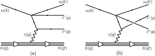
Figure 2: Feynman diagrams of the NTP processes in the SM and four momentum assignment.

III.1 Experimental Results

The muonic NTPs, $\nu_{\mu}\to\nu_{\mu}\mu\overline{\mu}$, has been measured by the CHARM-II Geiregat et al. (1990), CCFR Mishra et al. (1991) and NuTeV Adams et al. (2000) experiments. The results are given as the ratio of the observed cross section to the SM prediction, $\sigma_{\mathrm{SM}}$,

$$\frac{\sigma_{\mathrm{CHARM-II}}}{\sigma_{\mathrm{SM}}} =1.58\pm 0.57,$$ (8a)

$$\frac{\sigma_{\mathrm{CCFR}}}{\sigma_{\mathrm{SM}}} =0.82\pm 0.28,$$ (8b)

$$\frac{\sigma_{\mathrm{NuTeV}}}{\sigma_{\mathrm{SM}}} =0.72^{+1.73}_{-0.72}.$$ (8c)

The CHARM-II and CCFR results are consistent with the SM prediction within the error. The NuTeV result has relatively large uncertainty and includes null result. Therefore we use the CHARM-II and CCFR results for our analyses.

III.2 Amplitudes

From Eq. (2), the SM amplitude of the NTP processes in Fig. 2 is given by

$$\mathcal{M}_{\mathrm{SM}}=\frac{4e^{2}G_{F}}{\sqrt{2}}\big{[}\overline{u_{\nu}}(k^{\prime})\gamma^{\alpha}P_{L}u_{\nu}(k)\big{]}\big{[}\overline{u_{\ell}}(p)O^{\mu}_{\alpha}v_{\ell}(\overline{p})\big{]}\frac{1}{q^{2}}\braket{Q^{\prime}}{J_{\mu}(-q^{2})}{Q},$$ (9)

where $u_{\ell}~{}(v_{\ell})$ and $u_{\nu}$ are the spinor of charged (anti-)lepton and neutrino, respectively. The operator $O^{\mu}_{\alpha}$ represents the charged lepton current part which is defined by

$$O^{\mu}_{\alpha}=\gamma^{\mu}\frac{\mathrlap{\!\not{\phantom{p}}}p+\mathrlap{\!\not{\phantom{q}}}q+m_{\ell}}{(p+q)^{2}-m_{\ell}^{2}}\gamma_{\alpha}(g_{L}P_{L}+g_{R}P_{R})+\gamma_{\alpha}(g_{L}P_{L}+g_{R}P_{R})\frac{-\mathrlap{\!\not{\phantom{\overline{p}}}}\overline{p}-\mathrlap{\!\not{\phantom{q}}}q+m_{\ell}}{(\overline{p}+q)^{2}-m_{\ell}^{2}}\gamma^{\mu}.$$ (10)

where $m_{l}$ is the mass of the charged lepton. Throughout this paper, neutrinos are assumed to be massless. Note that $O^{\mu}_{\alpha}$ satisfies the current conservation condition, $q_{\mu}O^{\mu}_{\alpha}=0$ Fujikawa (1971). The operator $J_{\mu}$ in the braket product is the electromagnetic current for nucleus.

From Eqs. (9) and (10), the squared amplitude with summing over spins is obtained as

$$\sum_{\mathrm{spins}}|\mathcal{M}_{\mathrm{SM}}|^{2}=\frac{e^{4}G_{F}^{2}}{2q^{4}}j^{\alpha\beta}L_{\alpha\beta}^{\mu\nu}J_{\mu\nu},$$ (11)

where $j^{\alpha\beta}$, $L^{\mu\nu}_{\alpha\beta}$ and $J_{\mu\nu}$ represent neutrino, charged lepton and nucleus contributions, respectively. These tensors are defined as

$$j^{\alpha\beta} =8(k^{\alpha}{k^{\prime}}^{\beta}+k^{\beta}{k^{\prime}}^{\alpha}-k\cdot k^{\prime}g^{\alpha\beta}-i\epsilon^{\rho\alpha\sigma\beta}k_{\rho}k^{\prime}_{\sigma}),$$ (12a)

$$L^{\mu\nu}_{\alpha\beta} =4\mathrm{Tr}\big{[}(\mathrlap{\!\not{\phantom{p}}}p+m_{\ell})W^{\mu}_{\alpha}(g_{L}P_{L}+g_{R}P_{R})(\mathrlap{\!\not{\phantom{\overline{p}}}}\overline{p}-m_{\ell})V^{\nu}_{\beta}(g^{\ast}_{L}P_{L}+g^{\ast}_{R}P_{R})\big{]},$$ (12b)

$$J_{\mu\nu} =\braket{Q^{\prime}}{J_{\mu}(t)}{Q}\braket{Q}{J_{\nu}^{\dagger}(t)}{Q^{\prime}}.$$ (12c)

where $t$ is defined by $t=-q^{2}=-(Q^{\prime}-Q)^{2}$. For convenience, we express the contraction of three tensors as

$$j^{\alpha\beta}L_{\alpha\beta}^{\mu\nu}J_{\mu\nu}=|g_{L}|^{2}M_{L}+|g_{R}|^{2}M_{R}-(g_{L}g_{R}^{\ast}+g_{L}^{\ast}g_{R})M_{LR},$$ (13)

where the concrete forms of $M_{L},~{}M_{R}$ and $M_{LR}$ are given in Appendix A. Since the cross term of $g_{L}$ and $g_{R}$, $M_{LR}$, is proportional to $m_{\ell}^{2}$, it is sub-leading when the lepton mass $m_{\ell}$ is small compared to the energy scale of the NTP process. Each term in Eq. (13) is invariant under the exchange of the lepton momenta, $(p,k)\leftrightarrow(\overline{p},k^{\prime})$. Furthermore, under the exchange of either $p\leftrightarrow\overline{p}$ or $k\leftrightarrow k^{\prime}$, $M_{L}$ and $M_{R}$ are exchanged each other,

$$M_{L}^{\mu\nu}\longleftrightarrow M_{R}^{\mu\nu},$$ (14)

while $M_{LR}$ remains the same. The nucleus tensor, Eq. (12c), can be expressed in terms of a nuclear form factor. For spin-$0$ nucleus,

$$J_{\mu\nu}=Z^{2}(Q+Q^{\prime})_{\mu}(Q+Q^{\prime})_{\nu}|F(t)|^{2},$$ (15)

where $Z$ is the atomic number of nucleus, and $F(t)$ is the nuclear form factor given by

$$F(t) =4\pi\int_{0}^{\infty}drr^{2}\rho(r)\frac{\sin\sqrt{t}r}{\sqrt{t}r}.$$ (16)

and $\rho(r)$ is the nuclear density. The normalization condition for $\rho(r)$ is

$$4\pi\int_{0}^{\infty}drr^{2}\rho(r)=1,$$ (17)

and the integral variable $r$ is a distance from the center of nucleus.

According to Ref. Ballett et al. (2019a); Altmannshofer et al. (2019); Ballett et al. (2019b), the DUNE experiment will provide us a large number of NTP events, where liquid argon is used at the near detector. In our numerical analysis, we consider argon as the target nucleus. Following Ref. De Jager et al. (1974), we parametrize $\rho$ as

$$\rho(r)=\rho_{0}\frac{1+w\dfrac{r^{2}}{c^{2}}}{1+\exp\left(\dfrac{r-c}{z}\right)},$$ (18)

where $\rho_{0}$ is a normalization factor. The parameters are given as $c=3.73$fm, $z=0.62$fm, $w=-0.19$ for ⁴⁰Ar.

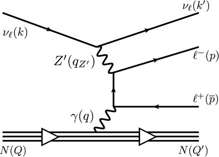
Figure 3: The $Z^{\prime}$ contribution of Feynman diagrams of NTP.

The $Z^{\prime}$ contribution to the NTP processes is shown in Fig. 3. The amplitude has the same spinor structure with Eq. (9). Only difference between the SM amplitude and the $Z^{\prime}$ amplitude is the propagator of $Z^{\prime}$ instead of $G_{F}$. Thus, the total amplitude squared of the NTP processes in our model, $|\mathcal{M}_{\mathrm{total}}|^{2}$, is obtained by simply replacing $g_{L}$ and $g_{R}$ in Eq. (12b) as

$$g_{L(R)}\to g_{L(R)}\mp\frac{\sqrt{2}}{4G_{F}}\frac{g^{\prime 2}}{q_{Z^{\prime}}^{2}-m_{Z^{\prime}}^{2}},$$ (19)

for $\nu_{\mu}\to\nu_{\mu}\mu\overline{\mu}$ ($-$) and $\nu_{\mu}\to\nu_{\mu}\tau\overline{\tau}$ ($+$). From Eq. (19), the NP parameter dependence disappears when

$$|q_{Z^{\prime}}^{2}|+m_{Z^{\prime}}^{2}\gg\frac{\sqrt{2}}{4G_{F}}{g^{\prime}}^{2}\simeq(157~{}\mathrm{MeV})^{2}\left(\frac{g^{\prime}}{9\times 10^{-4}}\right)^{2}.$$ (20)

As we will see in the next section, the $Z^{\prime}$ contribution is negligible in the tauonic NTP process. This fact suggests that $|q_{Z^{\prime}}^{2}|$ will become larger as the final state leptons are heavier. Then, the cross section is almost the same as that of the SM for the tauonic NTP process. In the next subsection, we show the dependence of the total cross section on the new physics parameter $g^{\prime}$ and $m_{Z^{\prime}}$.

III.3 Trident Production Cross Section

The total cross section of the NTP is given by

$$\sigma=\frac{1}{2(s-M^{2})}\int d\Pi\sum_{\mathrm{spins}}|\mathcal{M}_{\mathrm{total}}|^{2},$$ (21)

where $s=(k+Q)^{2}$ is the center of mass energy and $d\Pi$ is the phase space integral measure given by

$$d\Pi=\frac{d^{3}k^{\prime}}{(2\pi)^{3}2E_{k^{\prime}}}\frac{d^{3}p}{(2\pi)^{3}2E_{p}}\frac{d^{3}\overline{p}}{(2\pi)^{3}2E_{\overline{p}}}\frac{d^{3}Q^{\prime}}{(2\pi)^{3}2E_{Q^{\prime}}}(2\pi)^{4}\delta^{(4)}(k^{\prime}+p+\overline{p}+Q^{\prime}-k-Q).$$ (22)

By the energy-momentum conservations and rotational symmetry, the number of the integrals can be reduced from twelve to seven. Then, we perform the phase space integrations numerically using the changes of the integral variables shown in Appendix B.

The cross sections of muonic NTP in the minimal $L_{\mu}-L_{\tau}$ model are shown in Fig. 4. The left panel shows the cross sections with $m_{Z^{\prime}}=50,~{}100$ MeV and $g^{\prime}=5\times 10^{-4},~{}9\times 10^{-4}$ as a function of the incident neutrino energy $E_{\nu}$. The right panel shows the contours of the muonic NTP cross section in our model. In the left panel, the parameters, $(m_{Z^{\prime}},g^{\prime})$, are taken from the right panel as illustrating examples. Red curves correspond to $m_{Z^{\prime}}=100$ MeV and green ones to $50$ MeV, respectively. For comparison, we also show the cross section in the SM with the blue solid curve. Our results of the total cross section in the SM are in good agreement with previous studies Brown et al. (1972); Belusevic and Smith (1988) and Magill and Plestid (2017); Ballett et al. (2019a). It can be seen that the NP contributions become smaller compared with the SM cross section as $E_{\nu}$ becomes higher. This behavior generally holds even for $Z^{\prime}$ with much lighter mass than $E_{\nu}$. As we explained in the previous subsection, this is because $\left|q_{Z^{\prime}}^{2}\right|$ can take larger values than $m_{Z^{\prime}}^{2}$ for higher $E_{\nu}$, the NP contribution or the propagator of $Z^{\prime}$ decreases as $g^{\prime 2}/(G_{F}q_{Z^{\prime}}^{2})$. Thus, the cross section is less sensitive to the NP parameters for higher $E_{\nu}$, which has been shown in Ref. Kaneta and Shimomura (2017). Higher resolutions on momentum and/or energy measurements are required to solve the degeneracy in higher beam experiments like DUNE. On the other hand, for smaller $E_{\nu}$, the NP contributions to the cross section becomes larger, but the cross section itself becomes smaller. For example, for $E_{\nu}=1$ GeV, the cross section is $\mathcal{O}(10^{-44})$ cm².

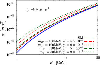
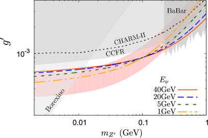
Figure 4: Left: Incident neutrino beam energy dependence of $\nu_{\mu}\to\mu_{\mu}\mu\overline{\mu}$ cross section in the $L_{\mu}-L_{\tau}$ model. Right: Contour plots of the same cross section for $\sigma=10^{-40}$ cm² in $m_{Z^{\prime}}$-$g^{\prime}$ plane.

In the right panel of Fig. 4, red, blue, green and orange curves correspond to the same cross sections for $E_{\nu}=40,~{}20,~{}5$ and $1$ GeV, respectively. We chose $(m_{Z}^{\prime},g^{\prime})=(0.1\,\text{GeV},9\times 10^{-4})$ as a reference parameter set to determine the values of the cross section. Thus all curves intersect at this point. The pink band represents muon $g-2$ favored region within $2\sigma$ and the gray shaded regions are excluded by Borexino Kaneta and Shimomura (2017), CHARM-II Geiregat et al. (1990), CCFR Mishra et al. (1991) and BaBar Lees et al. (2016). This plot clearly shows that the cross section is degenerate in $m_{Z^{\prime}}$ and $g^{\prime}$ over wide range. As we mentioned in the introduction, for the determination of the parameters, one needs additional information besides the cross section value.

$E_{\nu}$	$m_{Z^{\prime}}$	$g^{\prime}$	$\sigma$	$E_{\nu}$	$m_{Z^{\prime}}$	$g^{\prime}$	$\sigma$
$1$	—	—	$1.33\times 10^{-3}$	$20$	—	—	$1.8945$
	$0.020$	$5.869\times 10^{-4}$	$5.54\times 10^{-3}$		$0.020$	$7.009\times 10^{-4}$	$3.097$
	$0.10$	$9.000\times 10^{-4}$	$5.54\times 10^{-3}$		$0.10$	$9.000\times 10^{-4}$	$3.097$
	$0.20$	$1.299\times 10^{-3}$	$5.54\times 10^{-3}$		$0.20$	$1.111\times 10^{-3}$	$3.097$
	$1.0$	$4.972\times 10^{-3}$	$5.54\times 10^{-3}$		$1.0$	$2.824\times 10^{-3}$	$3.097$
$5$	—	—	$1.38\times 10^{-1}$	$40$	—	—	5.61
	$0.020$	$6.584\times 10^{-4}$	$0.328$		$0.020$	$7.18\times 10^{-4}$	$8.08$
	$0.10$	$9.000\times 10^{-4}$	$0.328$		$0.10$	$9.000\times 10^{-4}$	$8.08$
	$0.20$	$1.177\times 10^{-3}$	$0.328$		$0.20$	$1.084\times 10^{-3}$	$8.08$
	$1.0$	$3.632\times 10^{-3}$	$0.328$		$1.0$	$2.513\times 10^{-3}$	$8.08$

Table 2: Parameters for the same value of the cross sections for $\nu_{\mu}\to\mu_{\mu}\mu\overline{\mu}$. The units of $E_{\nu}$ and $m_{Z^{\prime}}$ are GeV, and that of $\sigma$ is $10^{-41}$ cm², respectively.

For this purpose, we analyze the distributions in the energies, opening angle and invariant mass of the final state charged leptons in the next section. The analyses are performed on the parameter sets shown in Table 2 for the muonic trident. The first row for each $E_{\nu}$ in Table 2 is the trident cross section in the SM. We chose $(m_{Z^{\prime}},g^{\prime})=(0.1$ GeV$,9\times 10^{-4})$ as a reference parameter, which can explain $(g-2)_{\mu}$ within $2\sigma$. Other parameter sets are chosen so that the cross sections have the same values with that of the reference set for each $E_{\nu}$. Note that some parameter sets are outside the $2\sigma$ region of $(g-2)_{\mu}$ or in the gray region. However, we include those parameter sets to see the behavior of the distributions for comparison.

$E_{\nu}$	$m_{Z^{\prime}}$	$g^{\prime}$	$\sigma$	$E_{\nu}$	$m_{Z^{\prime}}$	$g^{\prime}$	$\sigma$
$10$	—	—	$1.94\times 10^{-8}$	$40$	—	—	$1.87$
	$0.020$	$9.53\times 10^{-4}$	$1.98\times 10^{-8}$		$0.020$	$9.09\times 10^{-4}$	$1.87$
	$0.10$	$9.00\times 10^{-4}$	$1.96\times 10^{-8}$		$0.10$	$9.00\times 10^{-4}$	$1.87$
	$0.20$	$9.29\times 10^{-4}$	$1.95\times 10^{-8}$		$0.20$	$9.13\times 10^{-4}$	$1.87$
	$1.0$	$1.47\times 10^{-3}$	$1.94\times 10^{-8}$		$1.0$	$1.20\times 10^{-3}$	$1.87$

Table 3: Parameters for the same value of the cross section for $\nu_{\mu}\to\nu_{\mu}\tau\overline{\tau}$. The units of $E_{\nu}$ and $m_{Z^{\prime}}$ are GeV, and that of $\sigma$ is $10^{-47}$ cm², respectively.

We also show the cross sections of tauonic NTP, $\nu_{\mu}\to\nu_{\mu}\tau\overline{\tau}$, in Table 3 for $E_{\nu}=10$ and $40$ GeV. One finds that the cross sections for the reference point are almost the same as that in the SM. This suggests that the new physics contributions are very small. For tauonic trident to occur, the momentum transfer $|q_{Z^{\prime}}^{2}|$ will be of order $m_{\tau}^{2}$ and hence the new physics contribution is much suppressed as shown in Eq. (20). In fact, we have performed the same analyses for the tauonic NTP as for muonic one in the next section, and found that the distributions show tiny difference among the NP parameter sets in Table 3. Therefore, we show our numerical results only for muonic NTP in the next section.

IV Numerical Results

We show the distributions of the energies $E_{\mu}$ and $E_{\overline{\mu}}$, invariant mass $m^{2}_{\mu\overline{\mu}}$ and opening angle $\theta_{\mu\overline{\mu}}$ of muon and anti-muon in the SM and our model for the parameters given in Table 2. To obtain the total cross section of the NTP processes, we have to perform the phase space integral with a seven-dimension. For such high-dimensional integrals, the Monte Carlo integration is known to be useful due to its quick convergence compared to quadratures by parts.

To investigate the NP effect in the charged lepton distributions, we calculate the differential cross section with respect to some observables. In general, it is complicated to select an arbitrary observable as one of integral variables. However, when we use the Monte Carlo integration, we do not need to make the complicated variable transformation to obtain the differential cross section with respect to the favored observable.

Let $f(\bm{y})$ be a function of variables $\bm{y}$, which satisfies $\sigma=\int d\bm{y}f(\bm{y})$. Here, treating $\bm{y}$ as integral variables, we consider to perform the Monte Carlo integration. To obtain $d\sigma/dx$, we prepare discretized bins of a variable $x$, which are labeled by $a$ and have an interval $\Delta x_{a}$. In this integration, we sample the variables $\bm{y}$ from the uniform probability distribution $N$ times. At $i$-th step of the sampling, $x_{i}$ is calculated as well as $f(\bm{y}_{i})$ for generated $\bm{y}_{i}$. Then, one can approximate the distribution in the variable $x$ by

$$\frac{d\sigma}{dx}(x_{a})\simeq\frac{D}{N\Delta x_{a}}\sum_{i=1}^{N}f(\bm{y}_{i})\theta\left(x_{i}-x_{a}+\frac{\Delta x_{a}}{2}\right)\theta\left(x_{a}+\frac{\Delta x_{a}}{2}-x_{i}\right),$$ (23)

where $D$ is the total width of the $x$ bins and $N$ is the number of samples. The function $\theta(z)$ is a step function, which is a unity for $z\geq 0$ and zero for $z<0$. The total cross section can be obtained by summing Eq. (23) over $x$ as

$$\sigma\simeq\sum_{a}\Delta x_{a}\frac{d\sigma}{dx}(x_{a}).$$ (24)

IV.1 Energy Distributions

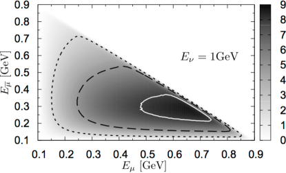
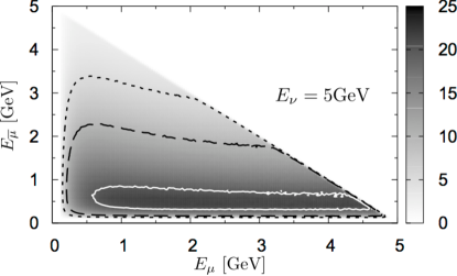
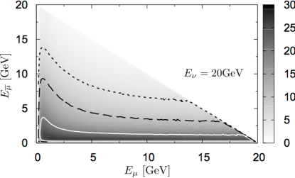
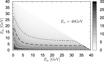
Figure 5: Contour plots of the distribution in $E_{\mu}$-$E_{\bar{\mu}}$ plane for $\nu_{\mu}\to\nu_{\mu}\mu\overline{\mu}$ in the SM. The color bar and contours are in unit of $10^{-44}$cm²/GeV². Solid (white), dashed (black) and dotted (black) curves are the contours of $8,~{}5$ and $2$ for $E_{\nu}=1$ GeV, and $20,~{}10$ and $5$ for $E_{\nu}=5,~{}20,~{}40$ GeV, respectively.

Firstly, we show the SM distributions of $E_{\mu}$ and $E_{\overline{\mu}}$ for the process of $\nu_{\mu}\to\nu_{\mu}\mu\overline{\mu}$ in Fig. 5. The energy of the incoming neutrino is taken to be $E_{\nu}=1,~{}5,~{}20$ and $40$ GeV, respectively. The color bar on the right indicates the value of the double differential cross section in unit of $10^{-44}$ cm²/GeV². Solid (white), dashed (black) and dotted (black) curves are the contours of $8,~{}5$ and $2$ in $10^{-44}$ cm²/GeV² for $E_{\nu}=1$ GeV, while $20,~{}10$ and $5$ in $10^{-44}$ cm²/GeV² for $E_{\nu}=5,~{}20,~{}40$ GeV, respectively.

In each panel, one can see that the distribution has a peak near the kinematical edge for $E_{\nu}=1$ GeV. As $E_{\nu}$ becomes higher, the peak moves to lower $E_{\mu}$ region. For $E_{\nu}>5$ GeV, $E_{\mu}$ is uniformly distributed rather than $E_{\overline{\mu}}$ is. We can understand this asymmetry of the distribution in $E_{\mu}$-$E_{\overline{\mu}}$ plane as follows: As we explained in Eq. (14), the terms $M_{L}$ and $M_{R}$ in the lepton tensor are exchanged under $p\leftrightarrow\overline{p}$. Thus, the double differential cross section differs under the exchange of $E_{\mu}\leftrightarrow E_{\overline{\mu}}$ if the coupling constants $g_{L}$ and $g_{R}$ are different as in the SM. It should be noticed that the distribution becomes symmetric in $E_{\mu}$-$E_{\overline{\mu}}$ plane for the case of $g_{L}=g_{R}$, such that the $L_{\mu}-L_{\tau}$ contributions dominate over the SM couplings.

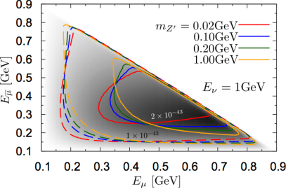
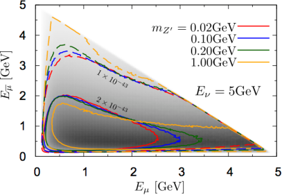
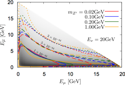
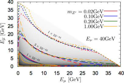
Figure 6: Contour plots of the deviation from the SM in the $E_{\mu}$-$E_{\bar{\mu}}$ distribution of $\nu_{\mu}\to\nu_{\mu}\mu\overline{\mu}$. Red, blue, green and orange curves correspond to the parameter sets in Table 2. Solid, dashed and dotted curves are the contours of $R(E_{\mu},E_{\overline{\mu}})$ with values indicated near each curve. Background gray color is the SM distribution shown in Fig. 5.

To see the parameter dependence of the NP model, we show the deviation of the differential cross section in our model from the SM, which is defined by

$$R(E_{\mu},E_{\overline{\mu}})\equiv\frac{d^{2}\sigma}{dE_{\mu}dE_{\overline{\mu}}}-\frac{d^{2}\sigma_{\mathrm{SM}}}{dE_{\mu}dE_{\overline{\mu}}}.$$ (25)

In Fig. 6, solid, dashed and dotted curves are the contours of $R(E_{\mu},E_{\overline{\mu}})$ while red, blue, green and orange colors represent the parameter sets in Table 2. In each panel, the values of $R(E_{\mu},E_{\overline{\mu}})$ are indicated near each curve, and only the $Z^{\prime}$ mass is shown to specify the parameter sets. The gray background represents the SM distribution shown in Fig. 5.

From Fig. 6, the parameter dependence can be seen clearly in the contours of $R(E_{\mu},E_{\overline{\mu}})$ in high $E_{\mu}$ or $E_{\overline{\mu}}$ region . The contours extend to larger values of $E_{\mu}$ or $E_{\overline{\mu}}$ as the $Z^{\prime}$ mass is heavier. It is also seen that $E_{\mu}$ is uniformly distributed rather than $E_{\overline{\mu}}$ is, due to the interference between the NP and SM contributions. We note that $R(E_{\mu},E_{\overline{\mu}})$ is positive for all ($E_{\mu},E_{\overline{\mu}}$) in $\nu_{\mu}\to\nu_{\mu}\mu\overline{\mu}$ in our calculation. The $L_{\mu}-L_{\tau}$ contribution to enhances $\nu_{\mu}\to\nu_{\mu}\mu\overline{\mu}$ because both $g_{L}$ and $g_{R}$ are effectively enlarged by the propagator of the $Z^{\prime}$ boson as seen in Eq. (19).

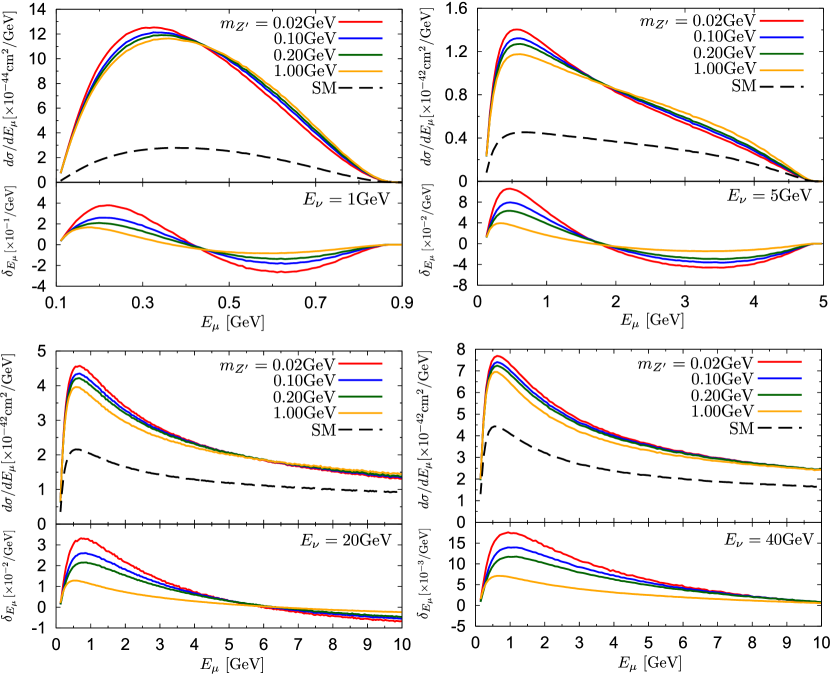
Figure 7: The $E_{\mu}$ distribution (upper panel) and shape of the distribution in $L_{\mu}-L_{\tau}$ model. Color of the curves are the same as Fig. 6. Black dashed curve represents the SM distribution.

Figure 7 and 8 show that the distributions (upper panel) and difference of shape of the distribution from the SM (lower panel) in $E_{\mu}$ and $E_{\overline{\mu}}$, respectively. Colors of the solid curves are the same in Fig. 6 and black dashed curve is the SM distribution. In the upper panels of Fig. 7, the parameter dependence of the distributions can be seen in two regions, around the peaks in lower $E_{\mu}$ and at tails in higher $E_{\mu}$. The parameter dependence is clearer around the peaks than at the tail. In each panels, one can see that the peaks become higher as the $Z^{\prime}$ mass is lighter. It is also seen that $E_{\mu}$ corresponding to the peak slightly differs among the parameter sets in each energy. On the other hand, in the upper panels of Fig. 8, the $E_{\overline{\mu}}$ distribution is less dependent on the parameters compared with the $E_{\mu}$ distributions. These results imply that the $E_{\mu}$ distribution is more useful to determine the new physics parameters.

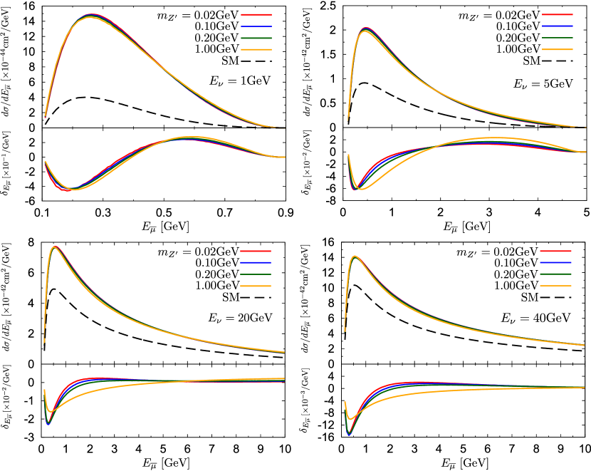
Figure 8: $E_{\overline{\mu}}$ distributions in $L_{\mu}-L_{\tau}$ model.

To see how the NP contributions modify the shape of the distributions, we define

$$\delta_{X}\equiv\frac{1}{\sigma}\frac{d\sigma}{dX}-\frac{1}{\sigma_{\mathrm{SM}}}\frac{d\sigma_{\mathrm{SM}}}{dX}.$$ (26)

for an arbitrary kenematical variable $X$. In the lower panels of Figs. 7 and 8, we plotted $\delta_{E_{\mu}}$ and $\delta_{E_{\overline{\mu}}}$, respectively. These are the difference of the normalized distributions, and become zero when the shape of the distributions are the same between our model and the SM, even if overall magnitudes are different. One can see in Fig. 7 that $\delta_{E_{\mu}}$ is positive in lower $E_{\mu}$ and negative in higher $E_{\mu}$ for all parameter sets. On the other hand, in Fig. 8, $\delta_{E_{\overline{\mu}}}$ shows the opposite behavior. Thus, the distributions are shifted to the lower $E_{\mu}$ and higher $E_{\overline{\mu}}$ by the NP contribution. The shape of the distribution also depends on the NP parameter set. In the $E_{\mu}$ distribution, $|\delta_{E_{\mu}}|$ is larger for the lighter $Z^{\prime}$ mass. Such information can be used to determine the parameters.

IV.2 Invariant Mass Distributions

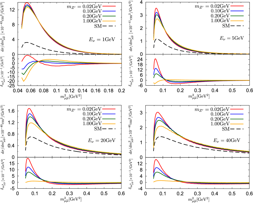
Figure 9: $m_{\mu\overline{\mu}}^{2}$ distributions in $L_{\mu}-L_{\tau}$ model.

The invariant mass of the outgoing muon and anti-muon is defined by

$$m^{2}_{\mu\overline{\mu}}\equiv(p+\overline{p})^{2}.$$ (27)

In Fig. 9, we show the invariant mass distribution (upper panel) and shape difference of this distribution from the SM (lower panel).

We can see from each panel that the distribution clearly depends on the parameters in lower value of $m^{2}_{\mu\overline{\mu}}$ region. The peaks of the distributions become sharper as the $Z^{\prime}$ mass is lighter and the dependence becomes more significant as $E_{\nu}$ is higher. It is also seen that the $m^{2}_{\mu\overline{\mu}}$ corresponding to the peak changes for the parameter sets. From the lower panels, one can also see that $\delta_{m^{2}_{\mu\overline{\mu}}}$, defined by Eq. 26, can take positive and negative values in lower value of $m^{2}_{\mu\overline{\mu}}$ depending on the parameters, which shows different behaviors from the energy distributions.

IV.3 Opening Angle Distributions

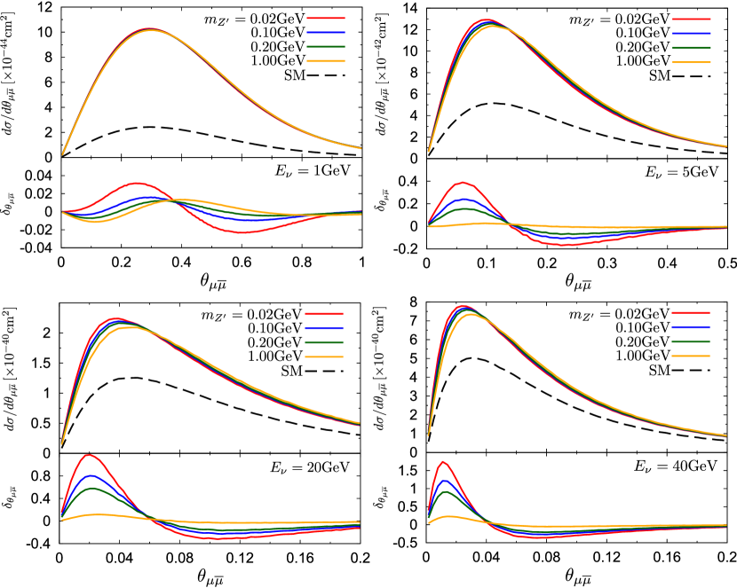
Figure 10: Muon opening angle distributions of the cross section in the $L_{\mu}-L_{\tau}$ model.

The opening angle of the outgoing muon and anti-muon can be defined by

$$\cos\theta_{\mu\overline{\mu}}\equiv\frac{\bm{p}\cdot\overline{\bm{p}}}{|\bm{p}||\overline{\bm{p}}|},$$ (28)

where $\bm{p}$ and $\overline{\bm{p}}$ are the momentum of muon and anti-muon, respectively. Figure 10 shows the distributions of $\theta_{\mu\overline{\mu}}$ (upper panel) and the shape (lower panel). From figure, one finds that the opening angle distributions shows the parameter dependence around the peaks for higher $E_{\nu}$. It is also seen that the angle for the peaks becomes smaller as $E_{\nu}$ becomes higher. Similar behavior can be seen in the shape of the distributions.

In this analysis, we have considered only the coherent NTP processes assuming argon as target material. Since the kinematical distributions depend on the form factor, the nuclear dependence is worth investigating for finding the best target material to identify the NP parameters.

We also understand that the diffractive NTP processes can be relevant for the available neutrino energy in experiments. We should check whether the diffractive contribution makes positive or negative effects for the measurement of NP parameters. We will study these topics in our future works.

V Summary

We have considered the minimal gauged $L_{\mu}-L_{\tau}$ model, and studied the dependences of the distributions of the neutrino trident production process on the new physics parameters, $m_{Z^{\prime}}$ and $g^{\prime}$. We analyzed the distributions of energies, opening angle and invariant mass of muons and their shapes in $\nu_{\mu}\to\nu_{\mu}\mu\overline{\mu}$.

We have found that the distributions can be different among the NP parameter sets for which the total cross sections are the same. In $E_{\mu}$-$E_{\overline{\mu}}$ distributions, the differences can be seen in larger $E_{\mu}$ or $E_{\overline{\mu}}$ region. We also found that the parameter dependences in the $E_{\mu}$ and $m_{\mu\overline{\mu}}^{2}$ distributions are rather clear compared with those in the $E_{\overline{\mu}}$ and $\theta_{\mu\overline{\mu}}$ distributions. Therefore the $E_{\mu}$ and $m_{\mu\overline{\mu}}^{2}$ distributions will be useful to determine the NP parameters. The shapes of the distributions were also presented, which shows the parameter dependence.

The determination of the new physics parameters by combining the information of the total cross section and distributions will be next step of our work. Such a study will need more detailed information including resolution and efficiencies in experiments. We leave such analyses for next work.

Appendix A Lepton Tensor

In this appendix, we present the analytic formula of the amplitude squared for $\nu_{\mu}\to\nu_{\mu}\ell\overline{\ell}$. The lepton and nucleus parts are written as a neutrino tensor $j^{\alpha\beta}$, charged lepton tensor $L_{\alpha\beta}^{\mu\nu}$, and nucleus tensor $J_{\mu\nu}$. Then, the amplitude squared is given by $j^{\alpha\beta}L^{\mu\nu}_{\alpha\beta}J_{\mu\nu}$ up to overall factors. Using the expression of the charged lepton tensor, (12b), it can be classified by the chirality of outgoing charged leptons as

$$j^{\alpha\beta}L_{\alpha\beta}^{\mu\nu}J_{\mu\nu}= \left|g_{L}\right|^{2}M_{L}+\left|g_{R}\right|^{2}M_{R}-g_{L}g_{R}^{*}M_{LR}-g_{L}^{*}g_{R}M_{RL},$$ (29)

where

$$M_{L}= 4J_{\mu\nu}j^{\alpha\beta}\mathrm{Tr}\left[\mathrlap{\!\not{\phantom{p}}}pW_{\alpha}^{\mu}\mathrlap{\!\not{\phantom{\overline{p}}}}\overline{p}V_{\beta}^{\nu}P_{L}\right],$$ (30)

$$M_{R}= 4J_{\mu\nu}j^{\alpha\beta}\mathrm{Tr}\left[\mathrlap{\!\not{\phantom{p}}}pW_{\alpha}^{\mu}\mathrlap{\!\not{\phantom{\overline{p}}}}\overline{p}V_{\beta}^{\nu}P_{R}\right],$$ (31)

$$M_{LR}= 4m_{\ell}^{2}J_{\mu\nu}j^{\alpha\beta}\mathrm{Tr}\left[W_{\alpha}^{\mu}V_{\beta}^{\nu}P_{R}\right],$$ (32)

$$M_{RL}= 4m_{\ell}^{2}J_{\mu\nu}j^{\alpha\beta}\mathrm{Tr}\left[W_{\alpha}^{\mu}V_{\beta}^{\nu}P_{L}\right].$$ (33)

Here, $W^{\mu}_{\alpha}$ and $V^{\nu}_{\beta}$ are the propagators of leptons given by

$$W_{\alpha}^{\mu}= \frac{2p^{\mu}+\gamma^{\mu}\mathrlap{\!\not{\phantom{q}}}q}{q^{2}+2p\cdot q}\gamma_{\alpha}-\gamma_{\alpha}\frac{2\overline{p}^{\mu}+\mathrlap{\!\not{\phantom{q}}}q\gamma^{\mu}}{q^{2}+2\overline{p}\cdot q}.$$ (34)

and

$$V_{\beta}^{\nu}= \gamma_{0}W_{\beta}^{\dagger\nu}\gamma_{0}=\gamma_{\beta}\frac{2p^{\nu}+\mathrlap{\!\not{\phantom{q}}}q\gamma^{\nu}}{q^{2}+2p\cdot q}-\frac{2\overline{p}^{\nu}+\gamma^{\nu}\mathrlap{\!\not{\phantom{q}}}q}{q^{2}+2\overline{p}\cdot q}\gamma_{\beta}.$$ (35)

Due to the parity conservation of the electomagnetic interaction, $J_{\mu\nu}$ must be symmetric with respect to $\mu$ and $\nu$, regardless of the detail of the nucleus. Thus, it is enough to calculate the symmetric part of $j^{\alpha\beta}L_{\alpha\beta}^{\mu\nu}$ under $\mu\leftrightarrow\nu$. The concrete form of the nucleus tensor $J_{\mu\nu}$ is determined by the target nucleus, as given in Eq. (15) with (18).

By the straightforward calculation, we obtain the explicit formula for $M_{L}$ in terms of lepton momenta as follows:

$$M_{L}= (-256J_{\mu\nu})\left\{\frac{M_{L1}^{\mu\nu}}{\left(q^{2}+2p\cdot q\right)^{2}}+\frac{M_{L2}^{\mu\nu}}{\left(q^{2}+2\overline{p}\cdot q\right)^{2}}+\frac{M_{L3}^{\mu\nu}}{\left(q^{2}+2p\cdot q\right)\left(q^{2}+2\overline{p}\cdot q\right)}\right\},$$ (36)

$$M_{L1}^{\mu\nu}= k\cdot\overline{p}\left[g^{\mu\nu}\left(2q\cdot k^{\prime}q\cdot p-q^{2}k^{\prime}\cdot p\right)+\left(p^{\mu}k^{\prime\nu}+p^{\nu}k^{\prime\mu}\right)\left(q^{2}+2p\cdot q\right)\right.$$

$$\hskip 28.45274pt\left.-2\left(p^{\mu}q^{\nu}+p^{\nu}q^{\mu}+2p^{\mu}p^{\nu}\right)\left\{k^{\prime}\cdot\left(p+q\right)\right\}\right],$$ (37)

$$M_{L2}^{\mu\nu}= \left(\text{$\{p,k\}\leftrightarrow\{\overline{p},k^{\prime}\}$ exchange of $M_{L1}^{\mu\nu}$}\right),$$ (38)

$$M_{L3}^{\mu\nu}= 2g^{\mu\nu}\left\{p\cdot q\left(k^{\prime}\cdot\overline{p}q\cdot k-q\cdot\overline{p}k\cdot k^{\prime}\right)\right.$$

$$\hskip 28.45274pt\left.+q\cdot k^{\prime}\left(q\cdot\overline{p}k\cdot p-p\cdot\overline{p}q\cdot k\right)+q^{2}\left(p\cdot\overline{p}k\cdot k^{\prime}-p\cdot k\overline{p}\cdot k^{\prime}\right)\right\}$$

$$+\left(p^{\mu}\overline{p}^{\nu}+p^{\nu}\overline{p}^{\mu}\right)\left(4k\cdot\overline{p}k^{\prime}\cdot p+2k\cdot qk^{\prime}\cdot q-q^{2}k\cdot k^{\prime}+2k\cdot\overline{p}q\cdot k^{\prime}+2k^{\prime}\cdot pq\cdot k\right)$$

$$+\left(p^{\mu}q^{\nu}+p^{\nu}q^{\mu}\right)\left(k\cdot\overline{p}q\cdot k^{\prime}+q\cdot\overline{p}k\cdot k^{\prime}-q\cdot kk^{\prime}\cdot\overline{p}+2k^{\prime}\cdot pk\cdot\overline{p}\right)$$

$$+\left(\overline{p}^{\mu}q^{\nu}+\overline{p}^{\nu}q^{\mu}\right)\left(k^{\prime}\cdot pq\cdot k+q\cdot pk\cdot k^{\prime}-q\cdot k^{\prime}k\cdot p+2k\cdot\overline{p}k^{\prime}\cdot p\right)$$

$$-\left(p^{\mu}k^{\nu}+p^{\nu}k^{\mu}\right)\left(2k^{\prime}\cdot pq\cdot\overline{p}+2q\cdot\overline{p}q\cdot k^{\prime}-q^{2}k^{\prime}\cdot\overline{p}\right)$$

$$-\left(\overline{p}^{\mu}k^{\prime\nu}+\overline{p}^{\nu}k^{\prime\mu}\right)\left(2k\cdot\overline{p}q\cdot p+2q\cdot pq\cdot k-q^{2}k\cdot p\right)$$

$$+\left(q^{\mu}k^{\nu}+q^{\nu}k^{\mu}\right)\left(p\cdot\overline{p}q\cdot k^{\prime}-k^{\prime}\cdot pq\cdot\overline{p}-k^{\prime}\cdot\overline{p}q\cdot p\right)$$

$$+\left(q^{\mu}k^{\prime\nu}+q^{\nu}k^{\prime\mu}\right)\left(p\cdot\overline{p}q\cdot k-k\cdot\overline{p}q\cdot p-k\cdot pq\cdot\overline{p}\right)$$

$$+\left(k^{\mu}k^{\prime\nu}+k^{\nu}k^{\prime\mu}\right)\left(2q\cdot pq\cdot\overline{p}-q^{2}p\cdot\overline{p}\right)$$

$$+\left(q^{\mu}q^{\nu}+q^{\nu}q^{\mu}\right)\left(k^{\prime}\cdot\overline{p}k\cdot p-k\cdot k^{\prime}p\cdot\overline{p}+k^{\prime}\cdot pk\cdot\overline{p}\right).$$ (39)

In the case of $V-A$ interaction, the amplitude squared is only $M_{L}$ which was given in Fujikawa (1971).

Nextly, moving on to the explicit form of $M_{R}$, one can easily derive it by taking the charge conjugate of materials in the trace:

$$M_{R}= 4J_{\mu\nu}j^{\alpha\beta}\mathrm{Tr}\left[\mathrlap{\!\not{\phantom{p}}}pW_{\beta}^{\nu}\mathrlap{\!\not{\phantom{\overline{p}}}}\overline{p}V_{\alpha}^{\mu}P_{L}\right]$$

$$= 4J_{\mu\nu}j^{\beta\alpha}\mathrm{Tr}\left[\mathrlap{\!\not{\phantom{p}}}pW_{\alpha}^{\mu}\mathrlap{\!\not{\phantom{\overline{p}}}}\overline{p}V_{\beta}^{\nu}P_{L}\right].$$ (40)

One notices that the form in the last line is the same as that of $M_{L}$ except for the superscripts of the neutrino tensor $j^{\alpha\beta}$. According to Eq. (12a), the exchange of $\mu$ and $\nu$ in $j^{\mu\nu}$ clearly corresponds to the exchange of $k$ and $k^{\prime}$. Therefore, $M_{R}$ is obtained as

$$M_{R}= \left(\text{$k\leftrightarrow k^{\prime}$ exchange of $M_{L}$}\right).$$ (41)

At last, we present $M_{LR}$ and $M_{RL}$. By using the explicit forms of $W_{\alpha}^{\mu}$ and $V_{\beta}^{\nu}$, one obtains $J_{\mu\nu}\mathrm{Tr}\left[W_{\alpha}^{\mu}V_{\beta}^{\nu}\gamma_{5}\right]=0$, which means $M_{LR}=M_{RL}$. Then, the terms are given by

$$M_{LR}=M_{RL}= (-256J_{\mu\nu})\left[\frac{M_{LR1}^{\mu\nu}}{\left(q^{2}+2p\cdot q\right)^{2}}+\frac{M_{LR2}^{\mu\nu}}{\left(q^{2}+2\overline{p}\cdot q\right)^{2}}+\frac{M_{LR3}^{\mu\nu}}{\left(q^{2}+2p\cdot q\right)\left(q^{2}+2\overline{p}\cdot q\right)}\right],$$ (42)

$$M_{LR1}^{\mu\nu}= \frac{m_{\ell}^{2}}{2}k\cdot k^{\prime}\left\{q^{2}g^{\mu\nu}+2\left[p^{\mu}q^{\nu}+p^{\nu}q^{\mu}\right]+4p^{\mu}p^{\nu}\right\},$$ (43)

$$M_{LR2}^{\mu\nu}= \left(\text{$p\leftrightarrow\overline{p}$ exchange of $M_{LR1}^{\mu\nu}$}\right),$$ (44)

$$M_{LR3}^{\mu\nu}= m_{\ell}^{2}\left[g^{\mu\nu}\left(2k\cdot qk^{\prime}\cdot q-q^{2}k\cdot k^{\prime}\right)-2k\cdot k^{\prime}\left(p^{\mu}\overline{p}^{\nu}+p^{\nu}\overline{p}^{\mu}\right)\right.$$

$$-k\cdot k^{\prime}\left(p^{\mu}q^{\nu}+p^{\nu}q^{\mu}+\overline{p}^{\mu}q^{\nu}+\overline{p}^{\nu}q^{\mu}\right)$$

$$\left.+q^{2}\left(k^{\mu}k^{\prime\nu}+k^{\nu}k^{\prime\mu}\right)-k^{\prime}\cdot q\left(k^{\mu}q^{\nu}+k^{\nu}q^{\mu}\right)-k\cdot q\left(k^{\prime\mu}q^{\nu}+k^{\prime\nu}q^{\mu}\right)\right].$$ (45)

When the incident neutrino is an anti-neutrino, the result can be obtained by replacing $k\leftrightarrow k^{\prime}$ in the above formulas. Note that the obtained transition density is invariant under the simultaneous replacement of $k\leftrightarrow k^{\prime}$ and $p\leftrightarrow\overline{p}$. These facts imply that the roles of emitted charged leptons are completely exchanged in the anti-neutrino case.

Appendix B Phase Space Integrals

We perform the Monte Carlo method in calculating the four-body phase space integral Czyz et al. (1964); Brown et al. (1972); Lovseth and Radomiski (1971). To achieve enough convergence of the integration, we choose suitable integral variables to flatten the integrand. The phase space integrals for the four-body final state are

$$d\Pi=\frac{d^{3}k^{\prime}}{(2\pi)^{3}2E_{k^{\prime}}}\frac{d^{3}p}{(2\pi)^{3}2E_{p}}\frac{d^{3}\overline{p}}{(2\pi)^{3}2E_{\overline{p}}}\frac{d^{3}Q^{\prime}}{(2\pi)^{3}2E_{Q^{\prime}}}\left(2\pi\right)^{4}\delta^{(4)}\left(k^{\prime}+p+\overline{p}+Q^{\prime}-k-Q\right).$$ (46)

Although the number of the integration variables are $3\times 4=12$, the net number is only eight because of the energy-momentum conservation.

In general, we can rewrite the phase space integral to

$$\int d\Pi= \int_{\underline{x}_{0}}^{\overline{x}_{0}}dx_{0}\int_{\underline{x}_{1}}^{\overline{x}_{1}}dx_{1}\int_{\underline{x}_{2}}^{\overline{x}_{2}}dx_{2}\int_{\underline{x}_{3}}^{\overline{x}_{3}}dx_{3}\int_{\underline{x}_{4}}^{\overline{x}_{4}}dx_{4}\int_{\underline{x}_{5}}^{\overline{x}_{5}}dx_{5}\int_{\underline{x}_{6}}^{\overline{x}_{6}}dx_{6}\int_{\underline{x}_{7}}^{\overline{x}_{7}}dx_{7}$$

$$\times X(x_{0},x_{1},x_{2},x_{3},x_{4},x_{5},x_{6},x_{7}),$$ (47)

where $X$ is an overall factor depending on the integral variables $x_{i}$ ($i=0,1,\cdots,7$). The upper and lower limits of $x_{i}$ are represented by $\overline{x}_{i}$ and $\underline{x}_{i}$, respectively. Since it is difficult to find the range of arbitrary integral variables, we have to choose a useful set of integral variables. In our analysis, we use the following set of the integral variables $x_{i}$s:

$$x_{0}= \phi_{Q^{\prime}}^{(A)},$$ (48)

$$x_{1}= \tau\equiv\int_{t}^{\infty}du\left\{F(u)\right\}^{2},$$ (49)

$$x_{2}= s_{p\overline{p}k}\equiv\left(p+\overline{p}+k^{\prime}\right)^{2},$$ (50)

$$x_{3}= s_{\overline{p}k}\equiv\left(\overline{p}+k^{\prime}\right)^{2},$$ (51)

$$x_{4}= u_{p}\equiv\log\left(-q^{2}-2p\cdot q\right),$$ (52)

$$x_{5}= \phi_{p}^{(B)},$$ (53)

$$x_{6}= u_{\overline{p}}\equiv\log\left(-q^{2}-2\overline{p}\cdot q\right),$$ (54)

$$x_{7}= \phi_{\overline{p}}^{(C)}.$$ (55)

$\phi_{Q^{\prime}}^{(A)}$, $\phi_{p}^{(B)}$, and $\phi_{\overline{p}}^{(C)}$ are rotation angles defined as follow: $\phi_{Q^{\prime}}^{(A)}$ is the rotation angle of $\bm{Q}^{\prime}$ around $\bm{k}$ in the center-of-mass frame of $\bm{k}$ and $\bm{Q}$, which we call the frame $A$. $\phi_{p}^{(B)}$ is the rotation angle of $\bm{p}$ around $\bm{q}$ in the frame where $\bm{p}+\overline{\bm{p}}+\bm{k}^{\prime}=0$, which we call the frame $B$. $\phi_{\overline{p}}^{(C)}$ is the rotation angle of $\overline{\bm{p}}$ around $\bm{q}$ in the frame where $\overline{\bm{p}}+\bm{k}^{\prime}=0$, which we call the frame $C$. This choice of variables is useful because all the three angles trivially run from $0$ to $2\pi$. Here, we obtain the overall factor,

$$X=\frac{\exp\left(u_{p}+u_{\overline{p}}\right)}{(4\pi)^{8}\left(s-M^{2}\right)\sqrt{s_{p\overline{p}k^{\prime}}s_{\overline{p}k^{\prime}}\left(t+\left|q_{0}^{\left(B\right)}\right|^{2}\right)\left(t+\left|q_{0}^{\left(C\right)}\right|^{2}\right)}\left\{F\left(t\right)\right\}^{2}}.$$ (56)

For the NTP processes, the differential cross sections have the rotational symmetry around the neutrino beam axis. Then, the integral of $\int d\phi_{Q^{\prime}}^{(A)}$ can be simply replaced by $2\pi$, and practically the other seven integral variables are relevant.

The variable $\tau$, defined by Eq. (49), runs over

$$\int_{t_{\mathrm{max}}}^{\infty}du\left\{F(u)\right\}^{2}<\tau<\int_{t_{\mathrm{min}}}^{\infty}du\left\{F(u)\right\}^{2},$$ (57)

where $t_{\mathrm{max}}$ ($t_{\mathrm{min}}$) is the maximum (minimum) value of $t=-q^{2}$. $t_{\mathrm{max}}$ and $t_{\mathrm{min}}$ are given by

$$t_{\mathrm{max}}= \frac{s}{2}\left(1-\frac{M^{2}}{s}\right)\left\{1-\frac{M^{2}}{s}+\sqrt{\lambda\left(1,\frac{M^{2}}{s},\frac{4m_{\ell}^{2}}{s}\right)}\right\}-2m_{\ell}^{2}\left(1+\frac{M^{2}}{s}\right),$$ (58)

$$t_{\mathrm{min}}= \frac{4m_{\ell}^{2}}{t_{\mathrm{max}}}\frac{M^{2}}{s},$$ (59)

Since we do not have the analytic representation of $t$ as a function of $\tau$, we prepare the numerical correspondence table between $t$ and $\tau$ for the phase space integration.

The ranges of the rest variables are as follows:

$$4m_{\ell}^{2}<s_{p\overline{p}k^{\prime}}< \frac{(s-M^{2})\sqrt{t\left(t-4M^{2}\right)}-\left(s+M^{2}\right)t}{2M^{2}},$$ (60)

$$m_{\ell}^{2}<s_{\overline{p}k^{\prime}}< \left(\sqrt{s_{p\overline{p}k^{\prime}}}-m_{\ell}\right)^{2},$$ (61)

$$\underline{u}_{p}= \log\left(t-\frac{s_{p\overline{p}k^{\prime}}-s_{\overline{p}k^{\prime}}+m_{\ell}^{2}}{\sqrt{s_{p\overline{p}k^{\prime}}}}q_{0}^{\left(B\right)}-\sqrt{s_{p\overline{p}k^{\prime}}\lambda\left(1,\frac{m_{\ell}^{2}}{s_{p\overline{p}k^{\prime}}},\frac{s_{\overline{p}k^{\prime}}}{s_{p\overline{p}k^{\prime}}}\right)\left(t+\left|q_{0}^{\left(B\right)}\right|^{2}\right)}\right),$$ (62)

$$\overline{u}_{p}= \log\left(t-\frac{s_{p\overline{p}k^{\prime}}-s_{\overline{p}k^{\prime}}+m_{\ell}^{2}}{\sqrt{s_{p\overline{p}k^{\prime}}}}q_{0}^{\left(B\right)}+\sqrt{s_{p\overline{p}k^{\prime}}\lambda\left(1,\frac{m_{\ell}^{2}}{s_{p\overline{p}k^{\prime}}},\frac{s_{\overline{p}k^{\prime}}}{s_{p\overline{p}k^{\prime}}}\right)\left(t+\left|q_{0}^{\left(B\right)}\right|^{2}\right)}\right),$$ (63)

$$\underline{u}_{\overline{p}}= \log\left(t-\frac{s_{\overline{p}k^{\prime}}+m_{\ell}^{2}}{\sqrt{s_{\overline{p}k^{\prime}}}}q_{0}^{\left(C\right)}-\frac{s_{\overline{p}k^{\prime}}-m_{\ell}^{2}}{\sqrt{s_{\overline{p}k^{\prime}}}}\sqrt{t+\left|q_{0}^{\left(C\right)}\right|^{2}}\right),$$ (64)

$$\overline{u}_{\overline{p}}= \log\left(t-\frac{s_{\overline{p}k^{\prime}}+m_{\ell}^{2}}{\sqrt{s_{\overline{p}k^{\prime}}}}q_{0}^{\left(C\right)}+\frac{s_{\overline{p}k^{\prime}}-m_{\ell}^{2}}{\sqrt{s_{\overline{p}k^{\prime}}}}\sqrt{t+\left|q_{0}^{\left(C\right)}\right|^{2}}\right),$$ (65)

where $q_{0}^{(B)}$ and $q_{0}^{(C)}$ are the time component of $q$ in the frame $B$ and $C$, respectively. In principle, we can derive the analytic formulas for $q_{0}^{(B)}$ and $q_{0}^{(C)}$, which are complicated a little. However, we do not need the analytic formulas because we easily obtain the numerical values of $q_{0}^{(B)}$ and $q_{0}^{(C)}$ step-by-step in the Monte Carlo integration. At each step, the upper and lower limit of $u_{p}$ are determined after $\tau$, $s_{p\overline{p}k^{\prime}}$, and $s_{\overline{p}k^{\prime}}$ are fixed. Then, the upper and lower limit of $u_{\overline{p}}$ are determined after $u_{p}$ and $\phi_{p}^{(B)}$ are fixed in addition.

References

- Bennett et al. (2006) G. W. Bennett et al. (Muon g-2), Phys. Rev. D73, 072003 (2006), eprint hep-ex/0602035.
- Tanabashi et al. (2018) M. Tanabashi et al. (Particle Data Group), Phys. Rev. D98, 030001 (2018).
- Blum et al. (2018) T. Blum, P. A. Boyle, V. Gülpers, T. Izubuchi, L. Jin, C. Jung, A. Jüttner, C. Lehner, A. Portelli, and J. T. Tsang (RBC, UKQCD), Phys. Rev. Lett. 121, 022003 (2018), eprint 1801.07224.
- Keshavarzi et al. (2018) A. Keshavarzi, D. Nomura, and T. Teubner, Phys. Rev. D97, 114025 (2018), eprint 1802.02995.
- Davier et al. (2020) M. Davier, A. Hoecker, B. Malaescu, and Z. Zhang, Eur. Phys. J. C 80, 241 (2020), [Erratum: Eur.Phys.J.C 80, 410 (2020)], eprint 1908.00921.
- Aoyama et al. (2020) T. Aoyama et al. (2020), eprint 2006.04822.
- Lindner et al. (2018) M. Lindner, M. Platscher, and F. S. Queiroz, Phys. Rept. 731, 1 (2018), eprint 1610.06587.
- Grange et al. (2015) J. Grange et al. (Muon g-2) (2015), eprint 1501.06858.
- Abe et al. (2019) M. Abe et al., PTEP 2019, 053C02 (2019), eprint 1901.03047.
- Foot (1991) R. Foot, Mod. Phys. Lett. A6, 527 (1991).
- He et al. (1991) X.-G. He, G. C. Joshi, H. Lew, and R. R. Volkas, Phys. Rev. D44, 2118 (1991).
- Foot et al. (1994) R. Foot, X. G. He, H. Lew, and R. R. Volkas, Phys. Rev. D50, 4571 (1994), eprint hep-ph/9401250.
- Altmannshofer et al. (2014a) W. Altmannshofer, S. Gori, M. Pospelov, and I. Yavin, Phys. Rev. Lett. 113, 091801 (2014a), eprint 1406.2332.
- Gninenko et al. (2015) S. Gninenko, N. Krasnikov, and V. Matveev, Phys. Rev. D 91, 095015 (2015), eprint 1412.1400.
- Kaneta and Shimomura (2017) Y. Kaneta and T. Shimomura, PTEP 2017, 053B04 (2017), eprint 1701.00156.
- Araki et al. (2017) T. Araki, S. Hoshino, T. Ota, J. Sato, and T. Shimomura, Phys. Rev. D 95, 055006 (2017), eprint 1702.01497.
- Chen and Nomura (2017) C.-H. Chen and T. Nomura, Phys. Rev. D 96, 095023 (2017), eprint 1704.04407.
- Nomura and Shimomura (2019) T. Nomura and T. Shimomura, Eur. Phys. J. C 79, 594 (2019), eprint 1803.00842.
- Banerjee and Roy (2019) H. Banerjee and S. Roy, Phys. Rev. D 99, 035035 (2019), eprint 1811.00407.
- Jho et al. (2019) Y. Jho, Y. Kwon, S. C. Park, and P.-Y. Tseng, JHEP 10, 168 (2019), eprint 1904.13053.
- Iguro et al. (2020) S. Iguro, Y. Omura, and M. Takeuchi (2020), eprint 2002.12728.
- Amaral et al. (2020) d. Amaral, Dorian Warren Praia, D. G. Cerdeno, P. Foldenauer, and E. Reid (2020), eprint 2006.11225.
- Araki et al. (2015) T. Araki, F. Kaneko, Y. Konishi, T. Ota, J. Sato, and T. Shimomura, Phys. Rev. D 91, 037301 (2015), eprint 1409.4180.
- Araki et al. (2016) T. Araki, F. Kaneko, T. Ota, J. Sato, and T. Shimomura, Phys. Rev. D 93, 013014 (2016), eprint 1508.07471.
- Asai et al. (2017) K. Asai, K. Hamaguchi, and N. Nagata, Eur. Phys. J. C 77, 763 (2017), eprint 1705.00419.
- Asai et al. (2019) K. Asai, K. Hamaguchi, N. Nagata, S.-Y. Tseng, and K. Tsumura, Phys. Rev. D 99, 055029 (2019), eprint 1811.07571.
- Asai (2020) K. Asai, Eur. Phys. J. C 80, 76 (2020), eprint 1907.04042.
- Araki et al. (2019) T. Araki, K. Asai, J. Sato, and T. Shimomura, Phys. Rev. D 100, 095012 (2019), eprint 1909.08827.
- Kamada et al. (2018) A. Kamada, K. Kaneta, K. Yanagi, and H.-B. Yu, JHEP 06, 117 (2018), eprint 1805.00651.
- Gninenko and Krasnikov (2018) S. Gninenko and N. Krasnikov, Phys. Lett. B 783, 24 (2018), eprint 1801.10448.
- Foldenauer (2019) P. Foldenauer, Phys. Rev. D 99, 035007 (2019), eprint 1808.03647.
- Asai et al. (2020) K. Asai, K. Hamaguchi, N. Nagata, and S.-Y. Tseng (2020), eprint 2005.01039.
- Ibe et al. (2017) M. Ibe, W. Nakano, and M. Suzuki, Phys. Rev. D 95, 055022 (2017), eprint 1611.08460.
- Han et al. (2019) Z.-L. Han, R. Ding, S.-J. Lin, and B. Zhu, Eur. Phys. J. C 79, 1007 (2019), eprint 1908.07192.
- Jho et al. (2020) Y. Jho, S. M. Lee, S. C. Park, Y. Park, and P.-Y. Tseng, JHEP 04, 086 (2020), eprint 2001.06572.
- Czyz et al. (1964) W. Czyz, G. Sheppey, and J. Walecka, Nuovo Cim. 34, 404 (1964).
- Lovseth and Radomiski (1971) J. Lovseth and M. Radomiski, Phys. Rev. D 3, 2686 (1971).
- Fujikawa (1971) K. Fujikawa, Annals Phys. 68, 102 (1971).
- Koike et al. (1971a) K. Koike, M. Konuma, K. Kurata, and K. Sugano, Prog. Theor. Phys. 46, 1150 (1971a).
- Koike et al. (1971b) K. Koike, M. Konuma, K. Kurata, and K. Sugano, Prog. Theor. Phys. 46, 1799 (1971b).
- Brown et al. (1972) R. Brown, R. Hobbs, J. Smith, and N. Stanko, Phys. Rev. D 6, 3273 (1972).
- Belusevic and Smith (1988) R. Belusevic and J. Smith, Phys. Rev. D 37, 2419 (1988).
- Altmannshofer et al. (2014b) W. Altmannshofer, S. Gori, M. Pospelov, and I. Yavin, Phys. Rev. D 89, 095033 (2014b), eprint 1403.1269.
- Geiregat et al. (1990) D. Geiregat et al. (CHARM-II), Phys. Lett. B245, 271 (1990).
- Mishra et al. (1991) S. R. Mishra et al. (CCFR), Phys. Rev. Lett. 66, 3117 (1991).
- Adams et al. (2000) T. Adams et al. (NuTeV), Phys. Rev. D 61, 092001 (2000), eprint hep-ex/9909041.
- Magill and Plestid (2017) G. Magill and R. Plestid, Phys. Rev. D 95, 073004 (2017), eprint 1612.05642.
- Magill and Plestid (2018) G. Magill and R. Plestid, Phys. Rev. D 97, 055003 (2018), eprint 1710.08431.
- Ballett et al. (2019a) P. Ballett, M. Hostert, S. Pascoli, Y. F. Perez-Gonzalez, Z. Tabrizi, and R. Zukanovich Funchal, JHEP 01, 119 (2019a), eprint 1807.10973.
- Altmannshofer et al. (2019) W. Altmannshofer, S. Gori, J. Martín-Albo, A. Sousa, and M. Wallbank, Phys. Rev. D 100, 115029 (2019), eprint 1902.06765.
- Ballett et al. (2019b) P. Ballett, M. Hostert, S. Pascoli, Y. F. Perez-Gonzalez, Z. Tabrizi, and R. Zukanovich Funchal, Phys. Rev. D 100, 055012 (2019b), eprint 1902.08579.
- de Gouvêa et al. (2019) A. de Gouvêa, P. J. Fox, R. Harnik, K. J. Kelly, and Y. Zhang, JHEP 01, 001 (2019), eprint 1809.06388.
- Ge et al. (2017) S.-F. Ge, M. Lindner, and W. Rodejohann, Phys. Lett. B 772, 164 (2017), eprint 1702.02617.
- Zhou and Beacom (2020a) B. Zhou and J. F. Beacom, Phys. Rev. D 101, 036011 (2020a), eprint 1910.08090.
- Zhou and Beacom (2020b) B. Zhou and J. F. Beacom, Phys. Rev. D 101, 036010 (2020b), eprint 1910.10720.
- De Jager et al. (1974) C. De Jager, H. De Vries, and C. De Vries, Atom. Data Nucl. Data Tabl. 14, 479 (1974), [Erratum: Atom.Data Nucl.Data Tabl. 16, 580–580 (1975)].
- Harnik et al. (2012) R. Harnik, J. Kopp, and P. A. Machado, JCAP 07, 026 (2012), eprint 1202.6073.
- Agarwalla et al. (2012) S. K. Agarwalla, F. Lombardi, and T. Takeuchi, JHEP 12, 079 (2012), eprint 1207.3492.
- Bilmis et al. (2015) S. Bilmis, I. Turan, T. Aliev, M. Deniz, L. Singh, and H. Wong, Phys. Rev. D 92, 033009 (2015), eprint 1502.07763.
- Lees et al. (2016) J. Lees et al. (BaBar), Phys. Rev. D 94, 011102 (2016), eprint 1606.03501.