In-Order Sliding-Window Aggregation in Worst-Case Constant Time

Abstract

Sliding-window aggregation is a widely-used approach for extracting insights from the most recent portion of a data stream. The aggregations of interest can usually be expressed as binary operators that are associative but not necessarily commutative nor invertible. Non-invertible operators, however, are difficult to support efficiently. In a 2017 conference paper, we introduced DABA, the first algorithm for sliding-window aggregation with worst-case constant time. Before DABA, if a window had size $n$, the best published algorithms would require $O(\log n)$ aggregation steps per window operation—and while for strictly in-order streams, this bound could be improved to $O(1)$ aggregation steps on average, it was not known how to achieve an $O(1)$ bound for the worst-case, which is critical for latency-sensitive applications. This article is an extended version of our 2017 paper. Besides describing DABA in more detail, this article introduces a new variant, DABA Lite, which achieves the same time bounds in less memory. Whereas DABA requires space for storing $2n$ partial aggregates, DABA Lite only requires space for $n+2$ partial aggregates. Our experiments on synthetic and real data support the theoretical findings.

1 Introduction

Table 1: Aggregation operators with their algebraic properties.

	Invertible	Associative	Commutative
Sum-like: sum, count, mean, geomean, stddev, …	✓	✓	✓
Max-like: max, min, argMax, maxCount, M4 jugel_et_al_2014 , …	$\times$	✓	$\times$
Mergeable sketch agarwal_et_al_2012 : Bloom, CountMin, HyperLogLog, algebraic classifiers izbicki_2013 , …	$\times$	✓	✓

Stream processing is a now-standard paradigm for handling high-speed continuous data, spurring the development of many stream-processing engines apache_flink_2016 ; akidau_et_al_2013 ; ali_et_al_2011 ; boykin_et_al_2014 ; cranor_et_al_2003 ; hirzel_et_al_2013 ; kulkarni_et_al_2015 ; murray_et_al_2013 ; toshniwal_et_al_2014 ; zaharia_et_al_2013 . Since stream processing is often subject to strict quality-of-service or real-time requirements, it requires low-latency responses. As a mainstay of stream processing, aggregation (e.g., computing the maximum, geometric mean, or more elaborate summaries such as Bloom filters bloom_1970 ) is one of the most common computations in streaming applications, used both standalone and as a building block for other analytics. Unfortunately, existing techniques for sliding-window aggregation cannot consistently guarantee low latency.

Because the newest data is often deemed more pertinent or valuable than older data, streaming aggregation is typically performed on a sliding window (e.g., the last hour’s worth of data). This not only provides intuitive semantics to the end users but also helps bound the amount of data the system has to keep around. Following Boykin et al. boykin_et_al_2014 , we use the term aggregation broadly, to include both classical relational aggregation operators such as sum, geometric mean, and maximum, as well as a more general class of associative operators. Table 1 lists several such operators and characterizes them by their algebraic properties. While some operators are invertible or commutative, many are not. This paper focuses on algorithms that work with all associative operators, including non-invertible and non-commutative ones.

An algorithm for sliding-window aggregation supports three operations (formally described in Section 2): insert for a data item’s arrival, query for requesting the current aggregation outcome, and evict for a data item’s departure hirzel_schneider_tangwongsan_2017 . This paper presents the De-Amortized Banker’s Aggregator (DABA), a novel general-purpose sliding-window aggregation algorithm that guarantees low-latency response on every operation—in the worst case, not just on average. The algorithm is simple and supports both fixed-sized and variable-sized windows. It works as long as (i) the aggregation operator, denoted by $\otimes$ in this paper, is an associative binary operator and (ii) the window has first-in first-out (FIFO) semantics. DABA does not require any other properties from the $\otimes$ operator. In particular, DABA works equally well whether $\otimes$ is invertible or non-invertible, commutative or non-commutative. DABA supports each of the query, insert, and evict operations by making at most a constant number of calls to the $\otimes$ operator in the worst case. This is independent of the window size, denoted by $n$ in this paper. If each invocation of $\otimes$ takes constant time, then the DABA algorithm takes worst-case constant time.

We first published the DABA algorithm in a 2015 technical report tangwongsan_hirzel_schneider_2015 and later in a 2017 conference paper tangwongsan_hirzel_schneider_2017 . Prior to the publication of DABA, the algorithms with the best algorithmic complexity for this problem in the published literature took $O(\log n)$ time arasu_widom_2004 ; tangwongsan_et_al_2015 , i.e., not $O(1)$ time like DABA. After the publication of DABA, there have been other papers with algorithms that take amortized $O(1)$ time for FIFO sliding-window aggregation shein_chrysanthis_labrinidis_2017 ; tangwongsan_hirzel_schneider_2019 ; theodorakis_et_al_2018 ; villalba_berral_carrera_2019 . However, these algorithms maintain the $O(1)$ time complexity only in the amortized sense, i.e., not in the worst case like DABA. In terms of space complexity, for a window of size $n$, DABA stores $2n$ partial aggregates. This journal version of the DABA paper also introduces a new, previously unpublished algorithm called DABA Lite that reduces the memory requirements to $n+2$ partial aggregates. Furthermore, this journal version has more extensive examples and visualizations for our algorithms.

The core idea behind DABA is to start from an algorithm that has amortized $O(1)$ time complexity and to de-amortize it. The algorithm that serves as a starting point is Two-Stacks. It uses an old trick from functional programming for representing a FIFO queue with two stacks, which we augment with aggregation. A special case of this algorithm was first mentioned in a Stack Overflow thread adamax_2011 . The Two-Stacks algorithm has one rare—but expensive—operation called flip that transfers all data from one stack to the other. The flip operation causes a latency spike, which can be undesirable for low-latency streaming. De-amortization turns the average-case $O(1)$ behavior of Two-Stacks into the worst-case $O(1)$ behavior of DABA by spreading out the expensive flip operation, thus eliminating the latency spike.

Two-Stacks, DABA, and DABA Lite only work for FIFO windows, i.e., for sliding windows over in-order streams. Handling out-of-order streams is beyond the scope of this paper. Indeed, it has been shown that the lower bound on the time complexity for aggregating out-of-order streams is worse than $O(1)$ unless disorder in a stream is bounded by a constant tangwongsan_hirzel_schneider_2019 . Before the emergence of constant-time sliding window aggregation algorithms, a popular approach for achieving low latency was to use coarse-grained windows where evictions occur in batches. This approach reduces the effective window size $n$, thus making algorithms whose time complexity depends on $n$ feasible. Pre-aggregating inside each batch reduces the cost of aggregating across batches carbone_et_al_2016 ; krishnamurthy_wu_franklin_2006 ; li_et_al_2005 . But coarse-grained windows are an approximation that does not always satisfy application requirements. Another popular research topic in sliding-window aggregation is window sharing, where aggregations for multiple different window sizes are computed on a single data structure. While some sliding window aggregation algorithms support window sharing in amortized $O(1)$ time, none of them achieve worst-case $O(1)$ time shein_chrysanthis_labrinidis_2017 ; tangwongsan_hirzel_schneider_2019 . DABA and DABA Lite achieve worst-case $O(1)$ time but do not support window sharing.

Experiments show that DABA and DABA Lite perform well in practice. We have implemented our new algorithms in C++ and benchmarked them against average-case $O(1)$ algorithms. True to being worst-case $O(1)$, our results show that DABA and DABA Lite have lower latency and competitive throughput as we increase the window size. When the aggregation operation is cheap, the low latency and high throughput are due to constant-time updates to a lightweight data structure. When the aggregation operation is expensive, they are due to a low-constant number of calls to the costly aggregation operator.

Our implementations of DABA, DABA Lite, and all other algorithms used in this paper are available on GitHub from the open source project Sliding Window Aggregators.

2 Problem Definition

This section formalizes the problem of maintaining aggregation in a first-in first-out (FIFO) sliding window and discusses the kinds of aggregations supported in this work.

2.1 Sliding-Window Aggregation Data Type

This paper is concerned with sliding-window aggregation on in-order streams with a first-in first-out (FIFO) window. In this type of window, the earliest data item to arrive is also the earliest data item to leave the window. Hence, the sliding window is a queue that supports aggregation of its data. The front of the queue contains the earliest data, the back of the queue holds the latest data, and the aggregation is from the earliest to the latest. As a queue, the window is only affected by two kinds of changes:

Data Arrival:

The arrival of a window data item results in a new data item at the end of the window. This is often triggered by the arrival of a data item in a relevant stream.

Data Eviction:

An eviction causes the data item at the front of the window to be removed from the window. The choice of when this happens is typically controlled by the window policy (e.g., a time-based window evicts the earliest data item when it falls out of the time frame of interest and a count-based window evicts the earliest data item to keep the size fixed gedik_2013 ). Window eviction policies are orthogonal to the algorithms in this paper.

We will model the problem of maintaining aggregation in a FIFO sliding window as an abstract data type (ADT) with an interface similar to that of a queue. To begin, we review an algebraic structure called a monoid:

Definition: A monoid is a triple $\mathcal{M}=(S,\otimes,\textbf{1})$ with a binary operator $\otimes\!:S\times S\to S$ on $S$ such that

• Associativity: For $a,b,c\in S$, $a\otimes(b\otimes c)=(a\otimes b)\otimes c$; and

• Identity: $\textbf{1}\in S$ is the identity: $\textbf{1}\otimes a=a=a\otimes\textbf{1}$ for all $a\in S$.

In comparison to real-number arithmetic, the $\otimes$ operator can be seen as a generalization of arithmetic multiplication where the identity element 1 is a generalization of the number $1$. Some of our earlier papers instead used an analogy to arithmetic addition with an identity element of zero. While that works equally well, here we adopt the multiplication analogy, because it makes it natural to adopt a shorthand notation of $abc$ for $a\otimes b\otimes c$. That shorthand makes it easier to write detailed examples.

A monoid is commutative if $a\otimes b=b\otimes a$ for all $a,b\in S$. A monoid has a left inverse if there exists a (known and reasonably cheap) function $\textit{inv}(\cdot)$ such that $a\otimes b\otimes\textit{inv}(a)=b$ for all $a,b\in S$. In general, a monoid may not be commutative nor invertible.

In the context of aggregation, monoids strike a good balance between generality and efficiency as was demonstrated before boykin_et_al_2014 ; tangwongsan_et_al_2015 ; yu_gunda_isard_2009 . For this reason, we focus our attention on supporting monoidal aggregation, formulating the abstract data type as follows:

Definition: The first-in first-out sliding-window aggregation (SWAG) abstract data type maintains a collection of window data and supports the following operations:

• $\mbox{\small{query}}()$ returns the ordered monoidal product of the window data. That is, if the sliding window contains values $v_{0},v_{1},\dots,v_{n-1}$ in their arrival order, query returns $v_{0}\otimes v_{1}\otimes\dots\otimes v_{n-1}$. If the window is empty, it returns 1.

• $\mbox{\small{insert}}(v)$ adds $v$ to the end of the sliding window. That is, if the sliding window contains values $v_{0},v_{1},\dots,v_{n-1}$ in their arrival order, then $\mbox{\small{insert}}(v)$ updates the collection to $v^{\prime}_{0},v^{\prime}_{1},\dots,v^{\prime}_{n}$, where $v^{\prime}_{i}=v_{i}$ for $i=0,1,\dots,n-1$ and $v^{\prime}_{n}=v$.

• $\mbox{\small{evict}}()$ removes the oldest item from the front of the sliding window. That is to say, if the sliding window contains values $v_{0},v_{1},\dots,v_{n-1}$ in their arrival order, then $\mbox{\small{evict}}()$ updates the collection to $v^{\prime}_{0},v^{\prime}_{1},\dots,v^{\prime}_{n-2}$, where $v^{\prime}_{i}=v_{i+1}$ for $i=0,1,2,\dots,n-2$.

Throughout, $n$ will denote the size of the current sliding window and $v_{0},v_{1},\dots,v_{n-1}$ will denote the contents of the sliding window in their arrival order, where $v_{0}$ is the oldest element. SWAG itself is not a concrete algorithm; it is merely an abstract data type, defining a set of operations with their expected behavior. The algorithms introduced in this paper (including Two-Stacks, DABA, and DABA Lite) are all concrete instantiations for the SWAG abstract data type.

2.2 Aggregation on Monoids

Despite their simplicity, monoids are expressive enough to capture most basic aggregations boykin_et_al_2014 ; tangwongsan_et_al_2015 , as well as more sophisticated aggregations such as maintaining approximate membership via a Bloom filter bloom_1970 , maintaining an approximate count of distinct elements flajolet_et_al_2007 , maintaining the versatile count-min sketch cormode_muthukrishnan_2005 , and indeed all operators in Table 1.

However, many aggregations (e.g., standard deviation) are not themselves monoids but can be couched as operations on a monoid with the help of two extra steps. To accomplish this, prior work tangwongsan_et_al_2015 gives a framework for the developer to provide three types In, Agg, and Out, and write three functions as follows:

• $\mbox{\small{lift}}(e:\mbox{\small{In}}):\mbox{\small{Agg}}$ takes an element of the input type and “lifts” it to an aggregation type that will be monoid operable.

• $\mbox{\small{combine}}(v_{1}:\mbox{\small{Agg}},v_{2}:\mbox{\small{Agg}}):\mbox{\small{Agg}}$ is a binary operator operating on the aggregation type. In our paper’s terminology, combine is the monoidal binary operator $\otimes$.

• $\mbox{\small{lower}}(v:\mbox{\small{Agg}}):\mbox{\small{Out}}$ turns an element of the aggregation type into an element of the output type.

Consider the example of maintaining the maxcount, which yields the number of times the maximal value occurs in the window. Define the type Agg as a pair $\langle m,c\rangle$ comprising the maximum $m$ and its count $c$. Then, define the three functions lift, combine, and lower as:

$$\mbox{\small{lift}}(e) =\langle m\mapsto e,c\mapsto 1\rangle$$

$$\mbox{\small{combine}}(v_{1},v_{2}) =\left\{\begin{array}[]{l@{\quad\textrm{if}\quad}l}v_{1}&v_{1}.m>v_{2}.m\\ v_{2}&v_{1}.m<v_{2}.m\\ \left\langle\begin{array}[]{l@{\,\mapsto\,}l}m&v_{1}.m,\\ c&v_{1}.c+v_{2}.c\end{array}\right\rangle&v_{1}.m=v_{2}.m\\ \end{array}\right.$$

$$\mbox{\small{lower}}(v) =v.c$$

It is easy to show that the combine function is an associative binary operator with identify element $\textbf{1}=\langle-\infty,0\rangle$. Consequently, $\mathcal{M}_{\textsf{maxcount}}=(\mbox{\small{Agg}},\mbox{\small{combine}},\langle-\infty,0\rangle)$ is a monoid.

In this framework, a query is conceptually answered as follows. If the sliding window currently contains the elements $e_{0},e_{1},\dots,e_{n-1}$, from the earliest to the latest, then lift derives $v_{i}=\mbox{\small{lift}}(e_{i})$ for $i=0,1,2,\dots,n-1$. Then, combine, rendered as infix $\otimes$, computes $v=v_{0}\otimes v_{1}\otimes\dots\otimes v_{n-1}$. Finally, lower produces the final answer as $\mbox{\small{lower}}(v)$.

Note that lift only needs to be applied to each element when it first arrives and lower to query results at the end. Therefore, the present paper focuses exclusively on the issue of maintaining the monoidal product—i.e., how to make as few invocations of combine as possible.

2.3 Example Trace

Using the maxcount monoid mentioned previously as a running example for the following sections, we will look at a trace of window operations and their effects on aggregations. Consider a window with the following contents, with the oldest element on the left and the youngest on the right.

4,

5,

3,

4,

0,

4,

4,

max=5, maxcount=1

The largest number in the window is 5, and it occurs only once, so the maxcount is 1. The oldest element on the left is 4, which is smaller than the current maximum 5, so evicting it does not affect the maximum or the maxcount.

5,

3,

4,

0,

4,

4,

max=5, maxcount=1

If we again evict the oldest element from the left, the maximum remaining window element becomes 4. Since the number 4 occurs thrice in the window, the maxcount is 3. The monoid is not invertible: this update could not have been accomplished by “subtracting out” information from the previous partial aggregate.

3,

4,

0,

4,

4,

max=4, maxcount=3

Inserting 2 does not affect the maximum, and hence, it also does not affect the maxcount.

3,

4,

0,

4,

4,

2,

max=4, maxcount=3

Finally, inserting 6 changes the maximum. Since the newly inserted element is the only 6 in the window, the maxcount becomes 1.

3,

4,

0,

4,

4,

2,

6,

max=6, maxcount=1

Notice that in this trace, insert and evict do not strictly alternate. In general, the SWAG data type, as well as all our algorithms, places no restrictions on how insert and evict may be called. They can be arbitrarily interleaved, allowing for dynamically-sized windows.

3 Two-Stacks

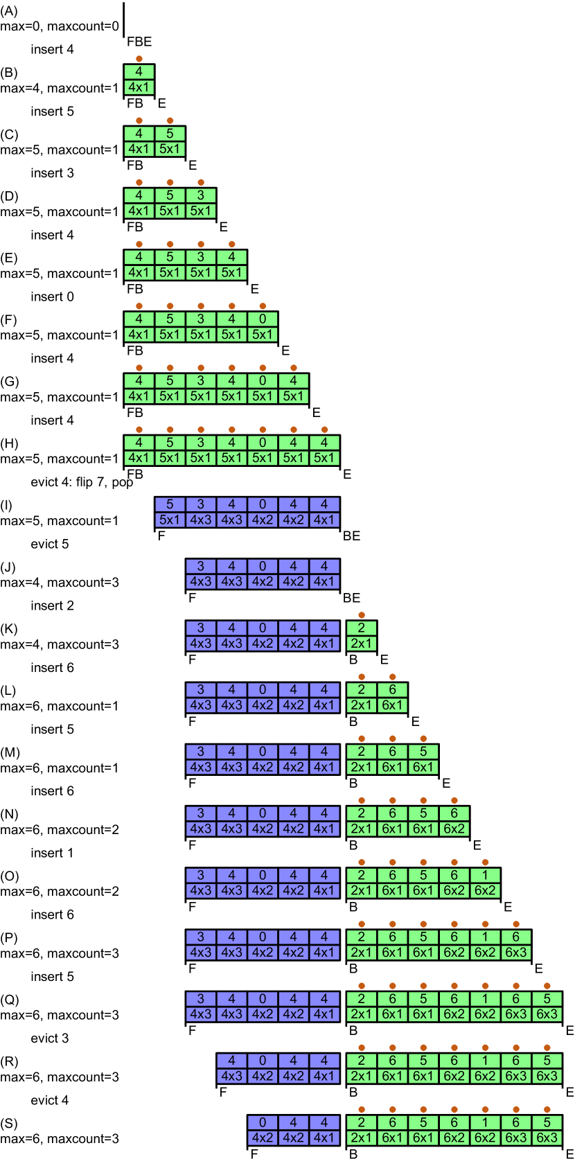
Figure 1: Two-Stacks example trace for maxcount aggregation. The notation $m\times c$ is shorthand for max=$m$, maxcount=$c$.

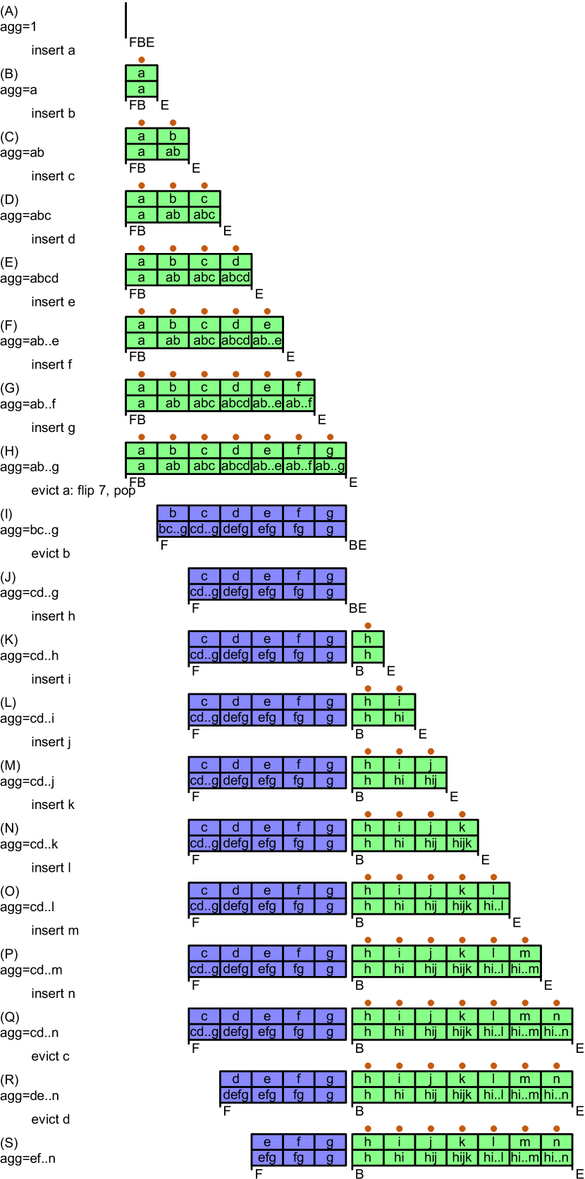
Figure 2: Two-Stacks example trace for any aggregation. The notation for aggregates omits $\otimes$, e.g., bc..g is shorthand for $\textsf{b}\otimes\textsf{c}\otimes\textsf{..}\otimes\textsf{g}$.

Two-Stacks is a simple algorithm for in-order sliding window aggregation (SWAG). For a window size $n$, it stores a total of $2n$ partial aggregates and implements each SWAG operation with amortized $O(1)$ and worst-case $O(n)$ invocations of $\otimes$.

The text of this section embeds several data-structure visualizations, which are all taken from concrete and complete example traces shown in Figs. 2 and 2.

Two-Stacks Data Structure.

As the name implies, the data structure for Two-Stacks comprises two stacks. We refer to them as the front stack $F$ and the back stack $B$. Here is an example of these two stacks for maxcount aggregation:

The front stack is shown in blue rotated $90^{\circ}$ left, with its top marked $F$ and its bottom marked $B$. The back stack is shown in green rotated $90^{\circ}$ right, with its bottom marked $B$ and its top marked $E$. To avoid clutter, the visualization only shows $B$ once to mark the bottoms of both the front stack and the back stack. As the window slides, evictions pop elements from the front stack on the left (at $F$) and insertions push elements on the back stack on the right (at $E$). Each stack element is a struct with two partial aggregates, val shown on top and agg shown on the bottom. The notation $4\times 3$ is shorthand for max=$4$, maxcount=$3$.

For amortized analysis, we use the banker’s (aka. accounting) method clrs_3rded , which keeps an imaginary savings account. In this method, every operation is amortized $O(1)$ if we can show that by billing the user a constant amount for every operation invoked, there is enough money at all time, without taking out a loan, to pay for the the actual work being done. We visualize the savings as small golden “coins” above the elements; they are not actual manifest in the data structure.

Two-Stacks Invariants.

An invariant for a data structure that implements in-order SWAG is a property that holds before and after every query, insert, or evict. Let $v_{0},\ldots,v_{n-1}$ be the lifted partial aggregates of the current window contents. Each val field stores the corresponding $v_{i}$. Each agg field stores the partial aggregate of the corresponding $v_{i}$ and all other values below it in the same stack. Formally, if $F[i]$ and $B[i]$ denote the $i^{\textrm{th}}$ element of $F$ and $B$ indexed from the left starting at index $0$:

$\begin{array}[]{l@{\;}l}&\forall i\in 0\ldots|F|-1:\;F[i].\mbox{\small{val}}=v_{i}\\ \textrm{and}&\forall i\in 0\ldots|F|-1:\;F[i].\mbox{\small{agg}}=v_{i}\otimes\ldots\otimes v_{|F|-1}\\ \textrm{and}&\forall i\in|F|\ldots|F|+|B|-1:B[i-|F|].\mbox{\small{val}}=v_{i}\\ \textrm{and}&\forall i\in|F|\ldots|F|+|B|-1:B[i-|F|].\mbox{\small{agg}}=v_{|F|}\otimes\ldots\otimes v_{i}\\ \end{array}$

The front stack aggregates to the right (easy eviction from the left). The back stack aggregates to the left (easy insertion from the right). Here is a visual example of the invariants:

The notation cd..g is shorthand for $\mbox{\small{c}}\otimes\mbox{\small{d}}\otimes\ldots\otimes\mbox{\small{g}}$. To work correctly regardless of commutativity, the aggregation in both stacks is ordered from the older elements on the left to newer elements on the right. For example, we take care to aggregate $\mbox{\small{f}}\otimes\mbox{\small{g}}$ instead of $\mbox{\small{g}}\otimes\mbox{\small{f}}$ because f is older than g.

Two-Stacks Algorithm.

Being an algorithm that implements in-order SWAG, Two-Stacks needs to define the functions query, insert, and evict. But first, we will define two private helper functions that retrieve the partial aggregate of the entire front stack $F$ and back stack $B$, respectively.

⬇

1fun $\Pi_{F}^{\otimes}$

2 if F.isEmpty() return 1 else return F.top().agg

3fun $\Pi_{B}^{\otimes}$

4 if B.isEmpty() return 1 else return B.top().agg

Recall that 1 is the identity element of the monoid. These helpers return the correct values in constant time, thanks to the invariants discussed previously. Function query combines the results of both helpers, using a single invocation of $\otimes$.

⬇

1fun query()

2 return $\Pi_{F}^{\otimes}$ $\otimes$ $\Pi_{B}^{\otimes}$

As an example, given the following data structure state, $\Pi_{F}^{\otimes}$ is $4\times 3$ and $\Pi_{B}^{\otimes}$ is $6\times 2$, so query returns the maximum $6\times 2$.

Next, to define insert and evict, we can assume that the invariants hold before function calls and must guarantee that they hold afterwards. The insert function just pushes onto $B$, taking constant time. Assuming the invariants hold for the old top of $B$, insert guarantees the invariants for the new top of $B$ by setting its partial aggregate agg to $\Pi_{B}^{\otimes}\otimes v$.

⬇

4fun insert($v$)

5 B.push($v$, $\Pi_{B}^{\otimes}$ $\otimes$ $v$)

The following example illustrates insert.

Finally, evict pops from $F$ after first ensuring that $F$ is nonempty.

⬇

2fun evict()

3 if F.isEmpty() # Flip

4 while not B.isEmpty()

5 F.push(B.top().val, B.top().val $\otimes$ $\Pi_{F}^{\otimes}$)

6 B.pop()

7 F.pop()

If $F$ is nonempty, then evict is trivial, for example:

On the other hand, if $F$ is empty, then evict must first do a flip. The flip operation pushes all values from $B$ onto $F$ and reverses the direction of the aggregation. In other words, it establishes that the agg fields satisfy the invariant for $F$. After the flip, evict simply does a pop as before.

Because of the reversal loop, flip takes $O(n)$ time, where $n$ is the current number of elements. Nevertheless, evict only takes amortized $O(1)$ time, as we will see below.

Two-Stacks Theorems.

Lemma 1

Two-Stacks maintains the invariants listed above.

Proof

The query function does not modify the stacks and thus does not change the invariants. The insert function maintains the invariants by correctly setting agg for the newly pushed element. The evict function maintains the invariants by correctly setting agg for all elements of $F$ during flip.  ∎

Theorem 3.1

If the window currently contains $v_{0},\ldots,v_{n-1}$, then query returns $v_{0}\otimes\ldots\otimes v_{n-1}$.

Proof

Using Lemma 1,

$\begin{array}[]{l@{\;}l@{\,\otimes\ldots\otimes\,}l@{\,\otimes\,}l@{\,\otimes\ldots\otimes\,}l}\lx@intercol\mbox{\small{query}}()\hfil\lx@intercol\\ =&\lx@intercol\Pi_{F}^{\otimes}\hfil\,\otimes\,&\lx@intercol\Pi_{B}^{\otimes}\hfil\lx@intercol\\ =&v_{0}&v_{|F|-1}&v_{|F|}&v_{|F|+|B|-1}\\ =&\lx@intercol v_{0}\otimes\ldots\otimes v_{n-1}\hfil\lx@intercol\end{array}$

∎

Theorem 3.2

Two-Stacks requires space to store $2n$ partial aggregates. Each call to query and insert invokes $\otimes$ exactly one time. Each call to evict invokes $\otimes$ at most $n$ times and amortized $1$ time.

Proof

The only part of the theorem that is not immediately obvious is the amortized complexity of evict. To see this, we bill each call to insert two imaginary coins: one for pushing an element onto $B$ and one to go into the savings. Hence, every element in $B$, as visualized, has a golden coin on top of it. When flip happens, it invokes $\otimes$ once for every element of $B$, which is completely paid for by spending the coin on that element. Because billing a constant amount per operation covers the total cost, each operation is amortized $O(1)$.   ∎

To summarize the workings of Two-Stacks, we will have another look at Figs. 2 and 2, which show complete example traces. Insertions push to the right of the back stack, visualized in green. Evictions pop from the left of the front stack, visualized in blue. Given an empty front stack, evict first performs a flip, as show in in Step (H)$\to$(I). The flip keeps values unchanged but reverses the associated partial aggregates. In this example, there are 7 partial aggregates to flip, coming from the preceding 7 insert operations, which have deposited 7 coins to the savings to pay for the flip.

4 Two-Stacks Lite

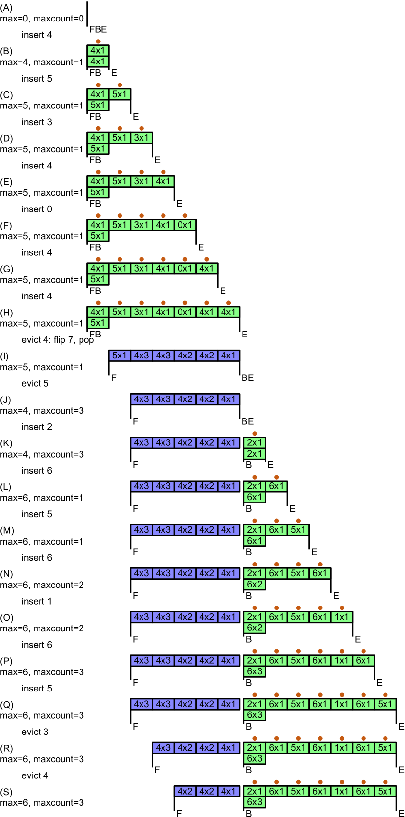
Figure 3: Two-Stacks Lite example trace for maxcount aggregation. The notation $m\times c$ is shorthand for max=$m$, maxcount=$c$.

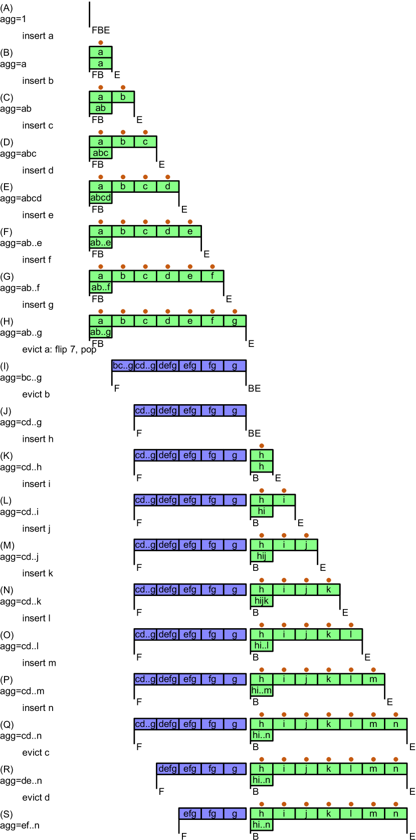
Figure 4: Two-Stacks Lite example trace for any aggregation. The notation for aggregates omits $\otimes$, e.g., bc..f is shorthand for $\textsf{b}\otimes\textsf{c}\otimes\textsf{..}\otimes\textsf{f}$.

Two-Stacks Lite improves upon Two-Stacks by reducing the space complexity from $2n$ down to $n+1$ stored partial aggregates. It does this by exploiting the insight that the Two-Stacks algorithm reads none of the val fields of the front stack and reads only the last agg field of the back stack. This idea comes from the Hammer Slide paper by Theodorakis et al. theodorakis_et_al_2018 . Another improvement is that instead of physically maintaining two separate stacks, Two-Stacks Lite maintains a single double-ended queue with an internal pointer $B$ to track the virtual stack boundary. The time complexity is unchanged, at amortized $O(1)$ and worst-case $O(n)$ invocations of $\otimes$ per SWAG operation. The data-structure visualizations in this section are taken from the concrete example traces shown in Figs. 4 and 4.

Two-Stacks Lite Data Structure.

The data structure for Two-Stacks Lite comprises a double-ended queue deque of partial aggregates, one additional partial aggregate aggB, and three pointers $F$, $B$, and $E$. Pointer $F$ points to the start of deque, $B$ points to a location between start and end, and $E$ points to the end. Here is an example with a max-count aggregation (the golden “coins” visualizing the savings serve the same purpose as in Two-Stacks):

Definition 1 (Pointers)

In this paper, a pointer is an iterator into a resizable double-ended queue that supports the following basic data structure operations:

• dereference and read or write contents: $v\leftarrow\texttt{*}p$, $\texttt{*}p\leftarrow v$

• pointer comparison: $p=q$, $p\neq q$

• pointer increment and decrement: $p+1$, $p-1$

• pointer assignment: $p\leftarrow q$

Our algorithms only use the above-listed pointer operations. These pointer operations can be implemented in worst-case $O(1)$ time over a variable-sized double-ended queue by implementing that queue using chunked arrays tangwongsan_hirzel_schneider_2015 . For stating invariants, we will also use a few additional pointer operations such as $p+i$, $p-q$, or $p<q$. These additional operations do not need to be $O(1)$ since they are used only by invariants and not directly by our algorithms.  ∎

Though physically the data structure uses a single deque, the pointers demarcate two virtual sublists, $l_{F}$ and $l_{B}$.

Two-Stacks Lite Invariants.

Let $v_{0},\ldots,v_{n-1}$ be the current window contents from the oldest to the youngest. Then, each deque element in the front sublist $l_{F}$ ($F\leq p<B$) stores the partial aggregate starting from the corresponding $v_{i}$ up to the element before $B$. Each deque element in the back sublist $l_{B}$ ($B\leq p<E$) stores the corresponding $v_{i}$. In addition, aggB stores the partial aggregate of all elements in $l_{B}$. Formally:

$\begin{array}[]{l@{\;}l}&\forall i\in 0\ldots B-F-1:\;\texttt{*}(F+i)=v_{i}\otimes\ldots\otimes v_{B-F-1}\\ \textrm{and}{}{}&\forall i\in B-F\ldots E-F-1:\;\texttt{*}(F+i)=v_{i}\\ \textrm{and}{}{}&\mbox{\small{aggB}}=\texttt{*}B\otimes\ldots\otimes\texttt{*}(E-1)\end{array}$

As an example, assume that the current window contains the values $v_{0}=\mbox{\small{c}}$, $v_{1}=\mbox{\small{d}}$, $v_{2}=\mbox{\small{e}}$, etc. up to $v_{10}=\mbox{\small{m}}$ and $v_{11}=\mbox{\small{n}}$. Then, if there are five elements in $l_{F}$ and seven in $l_{B}$, the data structure looks as follows:

The notation cd..g is shorthand for $\mbox{\small{c}}\otimes\mbox{\small{d}}\otimes\ldots\otimes\mbox{\small{g}}$.

Two-Stacks Lite Algorithm.

The private helper function $\Pi_{F}^{\otimes}$ retrieves the partial aggregate of the entire front sublist $l_{F}$, where 1 is the identity element of the monoid.

⬇

1fun $\Pi_{F}^{\otimes}$

2 if (F = B) return 1 else return *F

Function query obtains the partial aggregates of $l_{F}$ (by calling $\Pi_{F}^{\otimes}$) and of $l_{B}$ (by reading aggB) and combines them in constant time.

⬇

7fun query()

8 return $\Pi_{F}^{\otimes}$ $\otimes$ aggB

As an example, given the following data structure state, $\Pi_{F}^{\otimes}$ is $4\times 3$ and aggB is $6\times 2$, so query returns the maximum $6\times 2$.

Both insert and evict can assume that the invariants hold before they are called and must guarantee that they hold afterwards. Function insert$(v)$ accomplishes this by pushing $v$ and updating aggB accordingly.

⬇

2fun insert($v$)

3 deque.pushBack($v$)

4 E $\leftarrow$ E + 1

5 aggB $\leftarrow$ aggB $\otimes$ $v$

The following example illustrates insert.

Finally, evict pops from the front, after first ensuring that the front sublist $l_{F}$ is nonempty.

⬇

8fun evict()

9 if F = B and B $\neq$ E # Flip

10 I $\leftarrow$ E - 1

11 while I $\neq$ F

12 I $\leftarrow$ I - 1

13 *I $\leftarrow$ *I $\otimes$ *(I + 1)

14 B $\leftarrow$ E

15 aggB $\leftarrow$ 1

16 F $\leftarrow$ F + 1

17 deque.popFront()

If $l_{F}$ is nonempty, then evict is trivial, for example:

If $l_{F}$ is empty, then evict does a flip. Lines 11–14 rewrite the contents of deque in-place to contain partial aggregates from the corresponding element to the end. Line 15 updates pointer $B$ to indicate that the front sublist $l_{F}$ now occupies the entire data structure and the back sublist $l_{B}$ is empty. Then, Line 16 resets aggB to the monoid identity element. Here is a visualization of flip followed by pop:

The loop takes time $O(n)$ but can be amortized over the preceding $n$ insertions, where $n$ is the current window size.

Two-Stacks Lite Theorems.

Lemma 2

The Two-Stacks Lite algorithm maintains the Two-Stacks Lite invariants.

Proof

By inspection, function query preserves the data and thus the invariants. Function insert maintains the invariants by pushing $v$ and updating aggB. Function evict optionally does a flip, which reestablishes the invariants, then always does a pop, which also maintains the invariants.  ∎

Theorem 4.1

If the window currently contains $v_{0},\ldots,v_{n-1}$, then query returns $v_{0}\otimes\ldots\otimes v_{n-1}$.

Proof

Using Lemma 2,

$\begin{array}[]{l@{\;}l@{\,\otimes\ldots\otimes\,}l@{\,\otimes\,}l@{\,\otimes\ldots\otimes\,}l}\lx@intercol\mbox{\small{query}}()\hfil\lx@intercol\\ =&\lx@intercol\Pi_{F}^{\otimes}\hfil\,\otimes\,&\lx@intercol\mbox{\small{aggB}}\hfil\lx@intercol\\ =&v_{0}&v_{B-F-1}&v_{B-F}&v_{E-F-1}\\ =&\lx@intercol v_{0}\otimes\ldots\otimes v_{n-1}\hfil\lx@intercol\end{array}$

∎

Theorem 4.2

Two-Stacks Lite requires space to store $n+1$ partial aggregates. Each call to query and insert invokes $\otimes$ exactly one time. Each call to evict invokes $\otimes$ at most $n$ times and amortized one time.

Proof

Most of the theorem is obvious. To prove the amortized complexity of evict, bill each call to insert two imaginary coins for pushing an element onto the back and for the savings (visualized as small golden “coin” above the elements). Hence, every element in $l_{B}$ has a golden coin on top of it. When flip happens, it invokes $\otimes$ once for every element of $l_{B}$, which is completely paid for by spending the coin on that element.  ∎

5 DABA

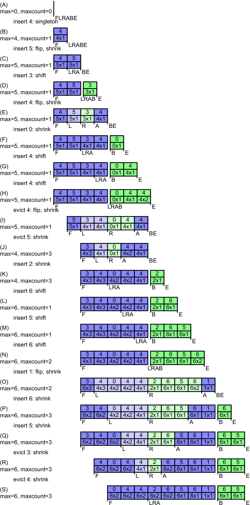
Figure 5: DABA example trace for maxcount aggregation. The notation $m\times c$ is shorthand for max=$m$, maxcount=$c$.

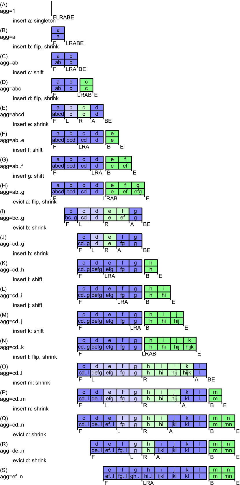
Figure 6: DABA example trace for any aggregation. The notation for aggregates omits $\otimes$, e.g., bc..f is shorthand for $\textsf{b}\otimes\textsf{c}\otimes\textsf{..}\otimes\textsf{f}$.

DABA is a low-latency algorithm for in-order sliding window aggregation (SWAG). When the window has size $n$, DABA requires space to store $2n$ partial aggregates and supports each SWAG operation using worst-case $O(1)$ invocations of $\otimes$. For a brief explanation of the name, DABA stands for De-Amortized Banker’s Aggregator: Amortization looks at the average cost of an operation over a long period of time. The banker’s method conceptualizes amortization as moving imaginary coins between the algorithm and a fictitious bank. Deamortization is a method that turns the average-case behavior into the worst-case behavior, usually by carefully spreading out expensive operations. In this spirit, notice that the expensive operation in the Two-Stacks algorithm is the loop for reversing the direction of aggregation during flip, paid for by imaginary coins deposited on preceding insertions. Whereas Two-Stacks does the flip late when the front stack becomes empty, DABA does the flip earlier, when the front and back stack reach the same length. Furthermore, instead of doing a reversal loop at the time of the flip, DABA spreads out the steps for reversing the direction of aggregation. The text of this section embeds several data-structure visualizations taken from concrete example traces shown in Figs. 6 and 6.

DABA Data Structure.

The DABA data structure comprises a double-ended queue, deque, and six pointers, $F$, $L$, $R$, $A$, $B$, and $E$, into that queue. Each queue element is a struct with two partial aggregates: val (top row) and agg (bottom row). The basic pointer operations are the same as in Definition 1 and are easy to implement in $O(1)$ time. The pointers are always ordered as follows:

$F\leq L\leq R\leq A\leq B\leq E$

Here is an example with a max-count aggregation:

The val fields store the window contents, with the $i^{\mathrm{th}}$ oldest value in FIFO order stored at $v_{i}=*(F+i).\mbox{\small{val}}$. The agg fields store partial aggregations over subranges of the window. Conceptually, each pointer $p$ corresponds to a sublist $l_{p}$. For example, pointer $F$ corresponds to sublist $l_{F}$. Each sublist is either aggregated to the left or to the right. The direction is carefully chosen to enable the DABA operations. The leftmost portion of the front list $l_{F}$ is aggregated to the left to facilitate eviction. The back list $l_{B}$ is aggregated to the right to facilitate insertion. The inner sublists $l_{L}$, $l_{R}$, and $l_{A}$ are designed to facilitate incremental reversal. Incremental reversal happens by adjusting the pointers demarcating sublist boundaries one step at a time. When a pointer moves, a deque element changes membership from one sublist to another and its agg field may need to be updated accordingly.

DABA Invariants.

DABA maintains three groups of invariants: values invariants, partial aggregate invariants, and size invariants. DABA’s values invariants specify that the val field of each element stores a singleton partial aggregate $v_{i}$ obtained by lifting the corresponding single stream element.

$\forall i\in 0\ldots E-F-1:*(F+i).\mbox{\small{val}}=v_{i}$

DABA’s partial aggregate invariants specify the contents of the agg fields before and after each SWAG operation, based on sublists. In the visualizations, blue indicates aggregation to the right and green indicates aggregation to the left. In the left-most portion of sublist $l_{F}$ (the front sublist, in dark blue), each agg field holds an aggregate starting from that element to the right end of $l_{F}$. In sublist $l_{L}$ (the left sublist, in light blue), each agg field holds an aggregate starting from that element to the right end of $l_{L}$. In sublist $l_{R}$ (the right sublist, in light green), each agg field holds an aggregate starting from the left end of $l_{R}$ to that element. In sublist $l_{A}$ (the accumulator sublist, in dark blue), each agg field holds an aggregate starting from that element to the right end of $l_{A}$, which coincides with the right end of $l_{F}$. Finally, in sublist $l_{B}$ (the back sublist, in dark green), each agg field holds an aggregate starting from the left end of $l_{B}$ to that element. Formally:

$\begin{array}[]{@{}ll@{:\,}l@{}}&\forall i\in 0\ldots L\!-\!F\!-\!1&*(F+i).\mbox{\small{agg}}=v_{i}\otimes\ldots\otimes v_{B-F-1}\\ \text{and}&\forall i\in L\!-\!F\ldots R\!-\!F\!-\!1&*(F+i).\mbox{\small{agg}}=v_{i}\otimes\ldots\otimes v_{R-F-1}\\ \text{and}&\forall i\in R\!-\!F\ldots A\!-\!F\!-\!1&*(F+i).\mbox{\small{agg}}=v_{R-F}\otimes\ldots\otimes v_{i}\\ \text{and}&\forall i\in A\!-\!F\ldots B\!-\!F\!-\!1&*(F+i).\mbox{\small{agg}}=v_{i}\otimes\ldots\otimes v_{B-F-1}\\ \text{and}&\forall i\in B\!-\!F\ldots E\!-\!F\!-\!1&*(F+i).\mbox{\small{agg}}=v_{B-F}\otimes\ldots\otimes v_{i}\\ \end{array}$

Here is a visual example of the invariants:

The notation cd..l is shorthand for $\mbox{\small{c}}\otimes\mbox{\small{d}}\otimes\ldots\otimes\mbox{\small{l}}$. To work correctly irrespective of whether the monoid is commutative or not, in all sublists, the operands of $\otimes$ are always ordered from older on the left to newer on the right.

DABA’s size invariants specify constraints on the sizes of sublists. Given a pointer $p$, we use the notation $|l_{p}|$ to indicate the size of sublist $l_{p}$. For example, the size of sublist $l_{F}$ is $|l_{F}|=B-F$ and the size of sublist $l_{L}$ is $|l_{L}|=R-L$. Formally, the size invariants are

$\Big{(}|l_{F}|=0\;\wedge\;|l_{B}|=0\Big{)}\vee\Big{(}{\color[rgb]{0,0,1}|l_{L}|+|l_{R}|+|l_{A}|+1=|l_{F}|-|l_{B}|}\;\wedge\;{\color[rgb]{.75,0,.25}|l_{L}|=|l_{R}|}\Big{)}$

This says that the window is either empty ($|l_{F}|=0$ and $|l_{B}|=0$) or the following two conditions hold:

• First, ${\color[rgb]{0,0,1}|l_{L}|+|l_{R}|+|l_{A}|+1\;=\;|l_{F}|-|l_{B}|}$. The size of the front list $l_{F}$ exceeds the size of the back list $l_{B}$ by the total size of the sublists $l_{L}$, $l_{R}$, and $l_{A}$ plus one. The sublists $l_{L}$, $l_{R}$, and $l_{A}$ are used for incremental reversal, and the algorithm, shown below, shrinks their total size by one on each insertion or eviction. When the sublists $l_{L}$, $l_{R}$, and $l_{A}$ are empty, the algorithm can make just one more insertion or eviction before $l_{F}$ and $l_{B}$ reach the same size. At that point, the algorithm does a flip, which relabels $l_{F}$ and $l_{B}$ into $l_{L}$ and $l_{R}$, respectively.

• Second, ${\color[rgb]{.75,0,.25}|l_{L}|=|l_{R}|}$. After each flip, $l_{L}$ and $l_{R}$ start out with the same size and then shrink at the same pace.

Below, we will see explanations for how the algorithm maintains these invariants, using color-coding to recognize corresponding subequations.

DABA Algorithm.

For each sublist $l_{p}$, a private helper function $\Pi_{p}^{\otimes}$ retrieves the corresponding partial aggregate or returns the monoid’s identity element 1 if the sublist is empty. Note that for a given sublist, we retrieve the partial aggregate in the left-most element if that sublist aggregates to the right, and the partial aggregate in the right-most element if that sublist aggregates to the left.

⬇

1fun $\Pi_{F}^{\otimes}$

2 if (F $=$ B) return 1 else return *F.agg

3fun $\Pi_{B}^{\otimes}$

4 if (B $=$ E) return 1 else return *(E-1).agg

5fun $\Pi_{L}^{\otimes}$

6 if (L $=$ R) return 1 else return *L.agg

7fun $\Pi_{R}^{\otimes}$

8 if (R $=$ A) return 1 else return *(A-1).agg

9fun $\Pi_{A}^{\otimes}$

10 if (A $=$ B) return 1 else return *A.agg

These helpers return the correct values in constant time, thanks to the invariants defined previously. Function query combines the aggregate of $l_{F}$ and $l_{B}$, taking only a single invocation of $\otimes$.

⬇

17fun query()

18 return $\Pi_{F}^{\otimes}$ $\otimes$ $\Pi_{B}^{\otimes}$

Function insert pushes a value $v$ with corresponding partial aggregate to the back of the deque, then calls a function fixup, defined below, for doing one step of incremental reversal.

⬇

10fun insert($v$)

11 deque.pushBack($v$, $\Pi_{B}^{\otimes}$ $\otimes$ $v$)

12 E $\leftarrow$ E + 1

13 fixup()

In our running maxcount example, if $\Pi_{B}^{\otimes}=0$ and $v=4$, then the newly pushed deque element has $\mbox{\small{val}}=4$ and $\mbox{\small{agg}}=4$.

Similarly, evict pops an element from the front of the deque, then calls fixup for one step of incremental reversal.

⬇

18fun evict()

19 F $\leftarrow$ F + 1

20 deque.popFront()

21 fixup()

In our running maxcount example, the following picture illustrates eviction:

The fixup function is responsible for restoring the invariants. Recall that we can assume that the following size invariants hold before each call to insert or evict:

$\Big{(}|l_{F}|=0\;\wedge\;|l_{B}|=0\Big{)}\vee\Big{(}{\color[rgb]{0,0,1}|l_{L}|+|l_{R}|+|l_{A}|+1=|l_{F}|-|l_{B}|}\;\wedge\;{\color[rgb]{.75,0,.25}|l_{L}|=|l_{R}|}\Big{)}$

Function insert grows $l_{B}$ by one element and function evict shrinks $l_{F}$ by one element. The impact on the invariants is the same in both cases: they both decrease the difference $|l_{F}|-|l_{B}|$ by one. Thanks to the extra $+1$ element in $l_{F}$, neither insert nor evict affects the inner sublists $l_{L}$, $l_{R}$, and $l_{A}$. This means that upon entry to fixup, the following is true:

$\Big{(}|l_{F}|=0\;\wedge\;|l_{B}|=1\Big{)}\vee\Big{(}{\color[rgb]{0,0,1}|l_{L}|+|l_{R}|+|l_{A}|=|l_{F}|-|l_{B}|}\;\wedge\;{\color[rgb]{.75,0,.25}|l_{L}|=|l_{R}|}\Big{)}$

Using the above as a precondition, the postcondition of fixup is to reestablish the original size invariants. The fixup function does this via four cases singleton, flip, shift, and shrink.

⬇

13fun fixup()

14 if F $=$ B # Singleton case

15 B $\leftarrow$ E, A $\leftarrow$ E, R $\leftarrow$ E, L $\leftarrow$ E

16 else

17 if L $=$ B # Flip

18 L $\leftarrow$ F, A $\leftarrow$ E, B $\leftarrow$ E

19 if L $=$ R # Shift

20 A $\leftarrow$ A + 1, R $\leftarrow$ R + 1, L $\leftarrow$ L + 1

21 else # Shrink

22 *L.agg $\leftarrow$ $\Pi_{L}^{\otimes}$ $\otimes$ $\Pi_{R}^{\otimes}$ $\otimes$ $\Pi_{A}^{\otimes}$

23 L $\leftarrow$ L + 1

24 *(A-1).agg $\leftarrow$ *(A-1).val $\otimes$ $\Pi_{A}^{\otimes}$

25 A $\leftarrow$ A - 1

The singleton case happens when $|l_{F}|=0$. Given the precondition, this can only hold when $|l_{B}|=1$. Then, without having to modify the deque, the pointer assignments

⬇

B $\leftarrow$ E, A $\leftarrow$ E, R $\leftarrow$ E, L $\leftarrow$ E

change the size of $l_{F}$ to $|l_{F}|=1$ while making all the other sublists $l_{L}$, $l_{R}$, $l_{A}$, and $l_{B}$ empty, as illustrated below.

The singleton case code thus establishes

$\Big{(}{\color[rgb]{0,0,1}|l_{L}|+|l_{R}|+|l_{A}|+1=|l_{F}|-|l_{B}|=1}\;\wedge\;{\color[rgb]{.75,0,.25}|l_{L}|=|l_{R}|=0}\Big{)}$

which implies the original size invariants.

The flip case happens when $|l_{F}|>0$ and the sublists for incremental reversal are empty: $|l_{L}|+|l_{R}|+|l_{A}|=0$. Together with the precondition, this implies that

$\Big{(}{\color[rgb]{0,0,1}|l_{L}|+|l_{R}|+|l_{A}|=0\wedge|l_{F}|=|l_{B}|}\;\wedge\;{\color[rgb]{.75,0,.25}|l_{L}|=0\wedge|l_{R}|=0\wedge|l_{A}|=0}\Big{)}$

Then, the pointer assignments

⬇

L $\leftarrow$ F, A $\leftarrow$ E, B $\leftarrow$ E

turn the old outer sublists $l_{F}$ and $l_{B}$ into the new inner sublists $l_{L}$ and $l_{R}$, respectively. No updates to agg fields are required because the corresponding sublists already have the correct aggregation direction.

After flip, the following holds:

$\Big{(}{\color[rgb]{0,0,1}|l_{L}|+|l_{R}|+|l_{A}|=|l_{F}|\wedge|l_{B}|=0}\;\wedge\;{\color[rgb]{.75,0,.25}|l_{L}|=|l_{R}|>0}\Big{)}$

At this point, we still need to execute the shrink case to repair the size invariants.

The shift case happens when $|l_{F}|>0$ and $|l_{L}|=0$. Together with the precondition, this implies that

$\Big{(}{\color[rgb]{0,0,1}|l_{L}|+|l_{R}|+|l_{A}|=|l_{F}|-|l_{B}|}\;\wedge\;{\color[rgb]{.75,0,.25}|l_{L}|=0\wedge|l_{R}|=0\wedge|l_{A}|>0}\Big{)}$

Then, the pointer assignments

⬇

A $\leftarrow$ A + 1, R $\leftarrow$ R + 1, L $\leftarrow$ L + 1

increment the pointers separating the left-most portion of $l_{F}$ from $l_{A}$ by one. No updates to agg fields are required because both the left-most portion of $l_{F}$ and $l_{A}$ are governed by the same aggs invariants.

After shift, the following holds:

$\Big{(}{\color[rgb]{0,0,1}|l_{L}|+|l_{R}|+|l_{A}|+1=|l_{F}|-|l_{B}|}\;\wedge\;{\color[rgb]{.75,0,.25}|l_{L}|=0\wedge|l_{R}|=0}\Big{)}$

which implies the original size invariants.

The shrink case happens when $|l_{F}|>0$ and $|l_{L}|>0$. There are two scenarios: with or without a flip from the same fixup. Either way, shrink starts with the following precondition:

$\Big{(}{\color[rgb]{0,0,1}|l_{L}|+|l_{R}|+|l_{A}|=|l_{F}|-|l_{B}|}\;\wedge\;{\color[rgb]{.75,0,.25}|l_{L}|=|l_{R}|\wedge|l_{L}|>0}\Big{)}$

The shrink case is the only part of fixup that modifies not just pointers but also agg fields. It reduces the sizes of both $l_{L}$ and $l_{R}$ by one each. The top element of $l_{L}$ becomes part of the left-most portion of $l_{F}$, so its agg field must be updated to $v_{L-F}\otimes\ldots\otimes v_{B-F}=\Pi_{L}^{\otimes}\otimes\Pi_{R}^{\otimes}\otimes\Pi_{A}^{\otimes}$. The top element of $l_{R}$ becomes part of the accumulator sublist $l_{A}$, so its agg field must be updated to $v_{A-F-1}\otimes\ldots\otimes v_{B-F}=v_{A-F-1}\otimes\Pi_{A}^{\otimes}$.

⬇

*L.agg $\leftarrow$ $\Pi_{L}^{\otimes}$ $\otimes$ $\Pi_{R}^{\otimes}$ $\otimes$ $\Pi_{A}^{\otimes}$

L $\leftarrow$ L + 1

*(A-1).agg $\leftarrow$ *(A-1).val $\otimes$ $\Pi_{A}^{\otimes}$

A $\leftarrow$ A - 1

The following is a typical example of shrink, reducing the sizes of $l_{L}$ and $l_{R}$ from 2 to 1.

The following is an example of flip followed by shrink. After the flip, $l_{L}$ and $l_{R}$ both have size 3. After the shrink, $l_{L}$ and $l_{R}$ both have size 2.

Given the precondition of shrink, it establishes the following postcondition:

$\Big{(}{\color[rgb]{0,0,1}|l_{L}|+|l_{R}|+|l_{A}|+1=|l_{F}|-|l_{B}|}\;\wedge\;{\color[rgb]{.75,0,.25}|l_{L}|=|l_{R}|}\Big{)}$

which implies the original size invariants.

DABA Intuitive View.

Now that we have seen all the small steps that make up DABA, let us look at their interplay to help understand the algorithm more holistically. Figs. 6 and 6 show two variants of the same example trace, differing only in their aggregation monoid. The sequence of cases starting at (D) comprises $[$flip shrink shrink shift shift$]$. A similar pattern starts at (H), comprising $[$flip shrink shrink shrink shift shift shift$]$. More generally, each flip is followed by an equal number of shrink^m and shift^m cases. For instance, the sequence starting at (B) is $[$flip shrink shift$]$, which is a special case where $m=1$. Visually, during the shrink^m phase of the algorithm, the light blue and light green sublists narrow to a point, looking like an upside-down step pyramid. This corresponds to the incremental reversal of $l_{R}$, which of course was $l_{B}$ before the flip. During the shrink^m phase, pointer $R$ does not change. Afterwards, during the shift^m phase, the $LRA$ pointers (which are now all the same) shift to the right one element at a time until they hit pointer $B$. When they reach $B$, the next insert or evict would cause $l_{F}$ and $l_{B}$ to have the same length, triggering the next flip and thus the next cycle. Within each cycle, pointer $B$ always stays the same; it only moves when a flip happens.

DABA Theorems.

Lemma 3

DABA maintains the invariants listed above, including the values invariants, the partial aggregate invariants, and the size invariants.

Proof

The query function does not modify the data structure and thus does not change the invariants. Functions insert and evict both establish the same precondition for fixup, as stated above. Finally, given that precondition, all cases of fixup reestablish the original invariants as a postcondition, as shown above.  ∎

Theorem 5.1

If the window currently contains $v_{0},\ldots,v_{n-1}$, then query returns $v_{0}\otimes\ldots\otimes v_{n-1}$.

Proof

Using Lemma 3,

$\begin{array}[]{l@{\;}l@{\,\otimes\ldots\otimes\,}l@{\,\otimes\,}l@{\,\otimes\ldots\otimes\,}l}\lx@intercol\mbox{\small{query}}()\hfil\lx@intercol\\ =&\lx@intercol\Pi_{F}^{\otimes}\hfil\,\otimes\,&\lx@intercol\Pi_{B}^{\otimes}\hfil\lx@intercol\\ =&v_{0}&v_{B-F-1}&v_{B-F}&v_{E-F-1}\\ =&\lx@intercol v_{0}\otimes\ldots\otimes v_{n-1}\hfil\lx@intercol\end{array}$

∎

Theorem 5.2

DABA requires space to store $2n$ partial aggregates. DABA invokes $\otimes$ at most one time per query, four times per insert, and three times per evict. Furthermore, for nonempty windows, DABA invokes $\otimes$ on average 2.5 times per insert and 1.5 times per evict.

Proof

The worst-case numbers can be seen directly from the code and by noting that the algorithm contains no loops or recursion. To see the average-case numbers, consider the sequence of fixup cases from a flip to the next. Immediately following flip, $l_{R}$ is nonempty and $l_{A}$ is empty. As long as $l_{R}$ is nonempty, each subsequent insert or evict executes a shrink, invoking $\otimes$ three times. When $l_{R}$ becomes empty, $l_{A}$ has exactly the size that $l_{R}$ had at the previous flip. As long as $l_{A}$ is nonempty, each subsequent insert or evict executes a shift, without invoking $\otimes$. The next flip happens when $l_{A}$ is empty. That means that there was an equal number of shrink steps as shift steps, and thus, an equal number of fixup calls with three invocations of $\otimes$ and with zero invocations of $\otimes$. This averages out to 1.5 $\otimes$-invocations per fixup, and thus, 2.5 $\otimes$-invocations per insert and 1.5 per evict.  ∎

A corollary of Theorem 5.2 is that DABA implements all SWAG operations with worst-case $O(1)$ invocations of $\otimes$. Unlike previous algorithms in the paper, DABA involves no costly steps that would require an amortization argument.

6 DABA Lite

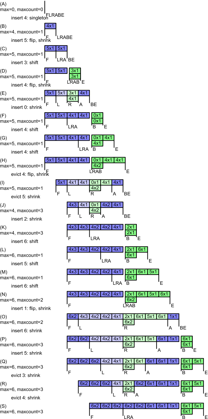
Figure 7: DABA Lite example trace for maxcount aggregation. The notation $m\times c$ is shorthand for max=$m$, maxcount=$c$.

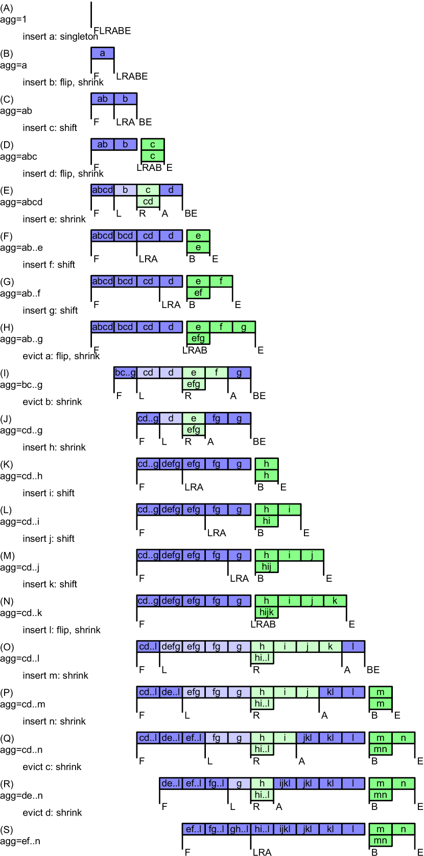
Figure 8: DABA Lite example trace for any aggregation. The notation for aggregates omits $\otimes$, e.g., bc..f is shorthand for $\textsf{b}\otimes\textsf{c}\otimes\textsf{..}\otimes\textsf{f}$.

DABA Lite improves upon the space complexity of DABA without increasing its running time, storing only $n+2$ partial aggregates, compared to $2n$ in DABA. It saves space by exploiting the insights that the DABA algorithm reads none of the val fields of the sublists that are aggregated to the left and only the last agg fields of sublists that are aggregated to the right. The time complexity is still worst-case $O(1)$ invocations of $\otimes$ per SWAG operation. The data-structure visualizations in this section are all taken from concrete example traces shown in Figs. 8 and 8.

DABA Lite Data Structure.

The DABA Lite data structure comprises a double-ended queue deque of partial aggregates, two additional partial aggregates aggRA and aggB, and six pointers $F$, $L$, $R$, $A$, $B$, and $E$ into the queue, see Definition 1. The pointers are always ordered as follows:

$F\leq L\leq R\leq A\leq B\leq E$

Here is an example with a max-count aggregation:

Conceptually, each pointer $p$ corresponds to a sublist $l_{p}$. Blue sublists are aggregated to the left to facilitate eviction, with each element containing the partial aggregate starting from that element to the right end of its sublist. The elements of green sublists simply contain the corresponding window elements. The aggregates for the green sublists are included in aggRA and aggB.

DABA Lite Invariants.

The contents invariants specify the contents of the deque and of aggRA and aggR. Let $v_{0},\ldots,v_{n-1}$ be the current window contents. In the leftmost portion of sublist $l_{F}$ (the front sublist, in dark blue), each element holds an aggregate starting from that element to the right end of $l_{F}$. In sublist $l_{L}$ (the left sublist, in light blue), each element holds an aggregate starting from that element to the right end of $l_{L}$. In sublist $l_{R}$ (the right sublist, in light green), each element holds the corresponding window element, and if $L\neq R$ then aggRA holds the combined partial aggregate of $l_{R}$ and $l_{A}$. In sublist $l_{A}$ (the accumulator sublist, in dark blue), each element holds an aggregate starting from that element to the right end of $l_{A}$. In sublist $l_{B}$ (the back sublist, in dark green), each element holds the corresponding window element, and aggB holds the aggregate of $l_{B}$. Formally:

$\begin{array}[]{@{}ll@{:\,}l@{}}&\forall i\in 0\ldots L-F-1&\texttt{*}(F+i)=v_{i}\otimes\ldots\otimes v_{B-F-1}\\ \text{and}&\forall i\in L-F\ldots R-F-1&\texttt{*}(F+i)=v_{i}\otimes\ldots\otimes v_{R-F-1}\\ \text{and}&\forall i\in R-F\ldots A-F-1&\texttt{*}(F+i)=v_{i}\\ \text{and}&\lx@intercol(L=R)\;\vee\;(\mbox{\small{aggRA}}=v_{R-F}\otimes\ldots\otimes v_{B-F-1})\hfil\lx@intercol\\ \text{and}&\forall i\in A-F\ldots B-F-1&\texttt{*}(F+i)=v_{i}\otimes\ldots\otimes v_{B-F-1}\\ \text{and}&\forall i\in B-F\ldots E-F-1&\texttt{*}(F+i)=v_{i}\\ \text{and}&\lx@intercol\mbox{\small{aggB}}=v_{B-F}\otimes\ldots\otimes v_{E-F-1}\hfil\lx@intercol\\ \end{array}$

Here is a visual example of the invariants for a window with contents $v_{0}=\mbox{\small{c}},v_{1}=\mbox{\small{d}},\ldots,v_{10}=\mbox{\small{m}},v_{11}=\mbox{\small{n}}$:

The notation cd..l is shorthand for $\mbox{\small{c}}\otimes\mbox{\small{d}}\otimes\ldots\otimes\mbox{\small{l}}$.

The size invariants specify constraints on the sizes of sublists. The size invariants of DABA Lite are the same as those of DABA:

$\Big{(}|l_{F}|=0\;\wedge\;|l_{B}|=0\Big{)}\vee\Big{(}{\color[rgb]{0,0,1}|l_{L}|+|l_{R}|+|l_{A}|+1=|l_{F}|-|l_{B}|}\;\wedge\;{\color[rgb]{.75,0,.25}|l_{L}|=|l_{R}|}\Big{)}$

DABA Lite Algorithm.

For each sublist $l_{p}$ that is aggregated to the left, a private helper function $\Pi_{p}^{\otimes}$ retrieves the corresponding partial aggregate or returns the monoid’s identity element 1 if the sublist is empty.

⬇

1fun $\Pi_{F}^{\otimes}$

2 if (F $=$ B) return 1 else return *F

3fun $\Pi_{L}^{\otimes}$

4 if (L $=$ R) return 1 else return *L

5fun $\Pi_{A}^{\otimes}$

6 if (A $=$ B) return 1 else return *A

These helpers return the correct values in constant time thanks to the invariants defined previously. Function query combines the aggregate of $l_{F}$ and $l_{B}$, taking only a single invocation of $\otimes$.

⬇

4fun query()

5 return $\Pi_{F}^{\otimes}$ $\otimes$ aggB

Function insert pushes a value $v$ onto $l_{B}$ and updates aggB accordingly, then calls a function fixup, defined below, for doing one step of incremental reversal.

⬇

6fun insert($v$)

7 deque.pushBack($v$)

8 E $\leftarrow$ E + 1

9 aggB $\leftarrow$ aggB $\otimes$ $v$

10 fixup()

In our running example, if $procName{aggB}=0\otimes 1$ and $v=4$, the newly pushed deque element is $4\otimes 1$ and the updated aggB is also $4\otimes 1$.

Similarly, evict pops an element from the front of the deque, then calls fixup for one step of incremental reversal.

⬇

5fun evict()

6 F $\leftarrow$ F + 1

7 deque.popFront()

8 fixup()

For our running example, eviction is illustrated below:

The fixup function repairs the invariants. The effect of fixup on the size invariants is the same for DABA and for DABA Lite. Since Section 5 has a formal analysis, here we only have an informal discussion. As before, the fixup function has four cases singleton, flip, shift, and shrink.

⬇

10fun fixup()

11 if F $=$ B # Singleton case

12 B $\leftarrow$ E, A $\leftarrow$ E, R $\leftarrow$ E, L $\leftarrow$ E

13 aggRA $\leftarrow$ 1

14 aggB $\leftarrow$ 1

15 else

16 if L $=$ B # Flip

17 L $\leftarrow$ F, A $\leftarrow$ E, B $\leftarrow$ E

18 aggRA $\leftarrow$ aggB

19 aggB $\leftarrow$ 1

20 if L $=$ R # Shift

21 A $\leftarrow$ A + 1, R $\leftarrow$ R + 1, L $\leftarrow$ L + 1

22 else # Shrink

23 *L $\leftarrow$ $\Pi_{L}^{\otimes}$ $\otimes$ aggRA

24 L $\leftarrow$ L + 1

25 *(A-1) $\leftarrow$ *(A-1) $\otimes$ $\Pi_{A}^{\otimes}$

26 A $\leftarrow$ A - 1

The singleton case happens when $|l_{F}|=0$ and $|l_{B}|=1$.

⬇

B $\leftarrow$ E, A $\leftarrow$ E, R $\leftarrow$ E, L $\leftarrow$ E

The pointer assignments change this to $|l_{F}|=1$ and $|l_{B}|=0$.

The flip case happens when $|l_{F}|>0$ and $|l_{L}|=0$ and $|l_{R}|=0$ and $|l_{A}|=0$. That implies that $|l_{F}|=|l_{B}|$, which means we can simply turn the old outer sublists $l_{F}$ and $l_{B}$ into the new inner sublists $l_{L}$ and $l_{R}$.

⬇

L $\leftarrow$ F, A $\leftarrow$ E, B $\leftarrow$ E

aggRA $\leftarrow$ aggB

aggB $\leftarrow$ 1

The corresponding updates to aggRA and aggB do not require any invocations of $\otimes$.

The shift case happens when $|l_{F}|>0$ and $|l_{L}|=0$. That means the pointers $L=R=A$ are equal, and can simply be moved one element to the right.

⬇

A $\leftarrow$ A + 1, R $\leftarrow$ R + 1, L $\leftarrow$ L + 1

There is no need to update aggRA, since it will not be read anymore until after the next flip. The invariant for aggRA remains satisfied, thanks to $L=R$.

The shrink case happens when $|l_{F}|>0$ and $|l_{L}|>0$. The sizes of $|l_{L}|=|l_{R}|$ are the same, and shrink reduces them by one each. This requires setting agg fields of blue sublists appropriately for their contents invariants.

⬇

*L $\leftarrow$ $\Pi_{L}^{\otimes}$ $\otimes$ aggRA

L $\leftarrow$ L + 1

*(A-1) $\leftarrow$ *(A-1) $\otimes$ $\Pi_{A}^{\otimes}$

A $\leftarrow$ A - 1

Even though the internal boundary $A$ between $l_{R}$ and $l_{A}$ moves, taken together, these two sublists still occupy the same elements, and thus, aggRA does not change. Consequently, the shrink case of DABA Lite requires one less $\otimes$-invocation than the shrink case of DABA.

The shrink case also gets triggered right after a flip.

DABA Lite Theorems.

Lemma 4

DABA Lite maintains both the contents invariants and the size invariants defined above.

Proof

The query function does not modify the data structure and thus does not change the invariants. The effect of insert, evict, and fixup on the size invariants is the same as for DABA. Whenever sublist boundaries change, the code updates the contents of deque, aggRA, and aggB, if necessary, to uphold the contents invariants.  ∎

Theorem 6.1

If the window currently contains $v_{0},\ldots,v_{n-1}$, then query returns $v_{0}\otimes\ldots\otimes v_{n-1}$.

Proof

Using Lemma 4,

$\begin{array}[]{l@{\;}l@{\,\otimes\ldots\otimes\,}l@{\,\otimes\,}l@{\,\otimes\ldots\otimes\,}l}\lx@intercol\mbox{\small{query}}()\hfil\lx@intercol\\ =&\lx@intercol\Pi_{F}^{\otimes}\hfil\,\otimes\,&\lx@intercol\mbox{\small{aggB}}\hfil\lx@intercol\\ =&v_{0}&v_{B-F-1}&v_{B-F}&v_{E-F-1}\\ =&\lx@intercol v_{0}\otimes\ldots\otimes v_{n-1}\hfil\lx@intercol\end{array}$

∎

Theorem 6.2

DABA Lite requires space to store $n+2$ partial aggregates. DABA Lite invokes $\otimes$ at most one time per query, three times per insert, and two times per evict. Furthermore, for nonempty windows, DABA Lite invokes $\otimes$ on average two times per insert and one time per evict.

Proof

The algorithm contains no loops or recursion, so we can directly see the worst-case numbers from the code. The average-case numbers are based on the observation that every sequence of shrink steps is followed by an equal number of shift steps. Shrink requires two $\otimes$-invocations and shift requires zero $\otimes$-invocations, so the average fixup call has one $\otimes$-invocation.  ∎

7 Experimental Evaluation

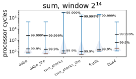
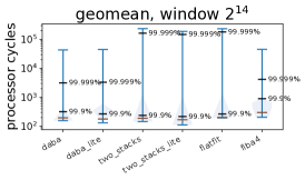
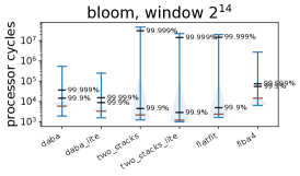
Figure 9: Latency, shown as violin plots, for static count-based windows with synthetic data.

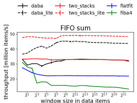
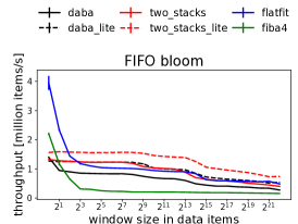
Figure 10: Throughput for static count-based windows with synthetic data.

The purpose of our experimental evaluation is to test whether DABA’s worst-case constant algorithmic complexity yields low latency and high throughput in practice, and to test whether DABA Lite is always more efficient than DABA.

Our experiments use six different SWAGs: Two-Stacks, Two-Stacks Lite, and FlatFIT shein_chrysanthis_labrinidis_2017 are all amortized $O(1)$, worst-case $O(n)$ algorithms designed for FIFO data. As originally published, FlatFIT does not support dynamic windows. We use a modified version that resizes FlatFIT’s circular buffer using the standard array doubling/shrinking technique without disturbing FlatFIT’s internal pointer structure. This results in an additional amortized $O(1)$ time per operation but supports dynamic windows and guarantees that the memory footprint is within a constant factor of the window size. We also adapted the published FlatFIT algorithm to our SWAG framework. DABA and DABA Lite are both worst-case $O(1)$ algorithms designed for FIFO data. FiBA tangwongsan_hirzel_schneider_2019 is designed for out-of-order data and reduces to amortized $O(1)$, worst-case $O(\log n)$ in the FIFO case. All of our experiments with FiBA use a min-arity of 4.

We chose three representative aggregation operators to span the execution cost spectrum. The operator sum is the sum of all items in the window, and it represents aggregation operations so cheap that the traversal and changes to the underlying data structure should dominate performance. The operator bloom applies a Bloom filter to all items in the window, and it represents aggregation operations where the operator itself dominates performance. The operator is so expensive that minimizing calls to it matters more than changes to the underlying data structure. Finally, geomean computes the geometric mean of all items in the window. It represents a middle ground of operator cost.

We implemented all algorithms in C++11, using the g++ compiler version 7.5.0 with optimization level -O3. Our system runs Red Hat 7.3, with Linux kernel version 3.10.0. The processor is an Intel Platinum 8168 at 2.7 GHz. All implementations, experiments, and post-processing scripts used in this section are available from the open-source project Sliding Window Aggregators.

7.1 Static Windows

The experiments in Figs 9 and 10 use a static count-based window with synthetic data. In each experiment, we first insert $n$ data items, where $n$ is the size of the window. The timed part of the experiment consists of rounds of evict, insert, and query. For the latency experiments, we record all times for 10 million rounds with a fixed window size of $2^{14}$ data items. For the throughput experiments, we time how long it takes to complete 200 million rounds, and we vary $n$ from 1 to $2^{22}$.

The practical reason to choose a worst-case $O(1)$ aggregator is to minimize latency. Both Two-Stacks and Two-Stacks Lite in Fig 9 tend to have lower minimum latency than both DABA and DABA Lite. But, true to their linear worst-case, Two-Stacks and Two-Stacks Lite regularly suffer from an order-of-magnitude higher latency. This trend becomes more pronounced as the cost of the aggregation function increases. Unlike the other aggregators, FiBA is tree based. As maintaining the tree is more up-front work, it tends to have high minimum and median latency. But, also being tree based, its worst-case behavior is bounded by $O(\log n)$; it has lower worst-case latency than the worst-case $O(n)$ aggregators. FlatFIT is not a tree-based structure, but the access pattern during queries ends up having similar properties: successive indirect accesses to different parts of the window. Each query pushes indices onto a stack, and then pops indices from the stack to indirectly access the window. This is a large amount of work, and when the aggregation operation is cheap, this work dominates performance and yields a high latency floor.

All of the aggregators are able to maintain close to constant behavior in Fig 10, although there are large differences between them. Surprisingly, DABA’s throughput is more competitive with Two-Stacks than in prior work tangwongsan_hirzel_schneider_2015 ; tangwongsan_hirzel_schneider_2017 . We attribute this difference to a more modern compiler with more aggressive inlining and dead-code elimination. Both DABA Lite and Two-Stacks Lite always outperform the corresponding non-Lite versions. FlatFIT becomes more competitive with expensive operations as its indirect accesses become less important compared to the total number of calls to the aggregation operation.

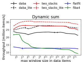
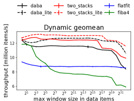
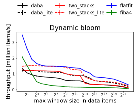
Figure 11: Throughput for dynamic count-based windows with synthetic data.

7.2 Dynamic Windows

The experiments in Fig. 11 use a dynamic count-based window with synthetic data. The experiments time a fill-and-drain pattern for a total of 200 million data items. It performs insert and query until reaching the window size $n$, and then calls evict until the window is down to 0, then repeats. We vary $n$ from 1 to $2^{22}$.

The throughput trends are largely the same as with static windows, which is the point of these experiments: even with dynamically changing window sizes, the fundamental properties of these streaming aggregation algorithms remain mostly the same. The one major difference is FlatFIT, whose throughput is consistently the best for bloom, which is the most expensive aggregation operation. This experimental design happens to be close to a best-case for FlatFIT, as it does not call the aggregation operation on evictions. FlatFIT only calls the aggregation operation on queries. The other algorithms require calling the aggregation operation on evictions in order to maintain their various properties of their partial aggregates. But, since the experiment performs no queries when it drains the window, such work is “wasted” in this case.

7.3 Real Data

The experiments in Fig. 12 use dynamic event-based windows based on real data. We use the dataset from the DEBS 2012 Grand Challenge debs2012_gc , which recorded data from manufacturing equipment at approximately 100 Hz. We removed about 1.5% of the 32.3 million events to enforce in-order data to make it suitable for FIFO aggregation algorithms. Our experiments maintain an event-time-based window of $\tau{}$ seconds, which means that the actual number of data items in that window will fluctuate over time. We do not start measuring until the window has evicted its first data item. In the throughput experiments, we vary $\tau$ from 10 milliseconds to 6 hours. In the latency experiments, we choose a window of 10 minutes. For both experiments, we use an aggregation operation inspired by Query 2 of the DEBS 2012 Grand Challenge: relative variation.

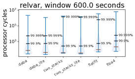
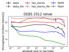
Figure 12: Throughput and latency for dynamic event-based windows with the manufacturing equipment data set.

Because FiBA was designed for out-of-order data, it natively has a concept of timestamps. But the other algorithms are FIFO aggregators and do not natively support timestamps. These sets of experiments use modified versions of all of the other aggregators that add support to query the youngest and oldest timestamps in the window. We use those queries to maintain the event-time window of $\tau{}$ seconds.

The results are consistent with the previous experiments, with two exceptions. First, DABA, DABA Lite, Two-Stacks, Two-Stacks Lite, and FlatFIT experience similar maximum latency, unlike with the static experiments. This latency similarity is caused by rare bulk evictions: rounds where more than 100 items are evicted experienced latencies more than 100$\times$ greater than the previous round. Since maintaining the same window is a shared property across all experiments, all algorithms have similar maximum latency. Second, the throughput of all algorithms experiences some degradation after $10^{3}$ seconds. This is because the actual window size is becoming a large enough fraction of the total data that rare events are not amortized.

7.4 Discussion

Our experiments demonstrate several consistent behaviors. The throughput of the Lite variants of both DABA and Two-Stacks are always significantly better than the original version, but the overall difference in latency is less dramatic. Two-Stacks Lite tends to have the best throughput. Since we lacked access to an implementation of FlatFIT by its authors, we re-implemented it based on their paper and extended it to support variable-sized windows. Our implementation of FlatFIT tends to have a high latency floor, but a median that is close to that floor. However, its maximum latency is consistent with being worst-case $O(n)$, and its throughput is only competitive with expensive operators or when the experiment happens to align with its design.

The theoretical analysis established that both DABA and DABA Lite are worst-case constant time algorithms. But low latency and competitive throughputs are sensitive to what the actual constant is. Our experiments demonstrate that DABA and DABA Lite are able to realize low latency and competitive throughput across a large range of $n$ with both static and dynamic windows and with real data.

8 Related Work

This section discusses the literature on sliding window aggregation algorithms with an emphasis on in-order streams and associative aggregation operators $\otimes$. As before, let $n$ be the window size.

8.1 Solutions to the Same Problem

Section 2 formalized the problem statement as an abstract data type called SWAG for first-in-first-out sliding window aggregation. This section discusses concrete algorithms that implement the abstract data type. Section 2 phrased associative aggregation operators as monoids. While some monoids are invertible or commutative, that is not true for all monoids, and thus, this section only lists algorithms that work without such additional algebraic properties. This section presents algorithms in chronological order by publication date.

Recalculate-from-scratch implements SWAG by maintaining a FIFO queue of all data items and calculating the aggregation of the entire queue for each query. Each query requires $O(n)$ invocations of $\otimes$. The queue takes up space for $n$ data stream values.

The B-Int algorithm from 2004 arasu_widom_2004 implements SWAG using base intervals, which are similar to a balanced binary tree. The time complexity is $O(\log n)$ invocations of $\otimes$ and the space complexity is around $2n$ partial aggregates: $n$ for leaves plus $\sim n$ for internal nodes.

The Two-Stacks idea was mentioned in a Stack Overflow post from 2011 adamax_2011 , which described the idea for one aggregation operator, minimum. Even though Two-Stacks is a SWAG algorithm, it was not immediately noticed as such by the academic community. As discussed in Section 3, the time complexity is amortized $O(1)$ invocations of $\otimes$ with a worst-case of $O(n)$, and the space is $2n$ partial aggregates.

The Reactive Aggregator from 2015 implements SWAG using a perfect binary tree. This algorithm uses a data structure called FlatFAT, which stands for flat fixed-sized aggregator and represents a perfect binary tree without storing explicit pointers and without needing any rebalancing. The time complexity is amortized $O(\log n)$ with a worst-case of $O(n)$ invocations of $\otimes$. If $n$ is a power of two, FlatFAT requires space for $\sim 2n$ partial aggregates: $n$ leaves plus $n$ interior nodes. If $n$ is slightly above a power of two, the space can be up to $\sim 4n$.

The DABA algorithm was first published in 2015 tangwongsan_hirzel_schneider_2015 . DABA was inspired by Okasaki’s purely functional queues and deques okasaki_1995 . However, the two differ substantially: DABA is not a purely functional data structure, and Okasaki’s data structures do not implement sliding window aggregation. As discussed in Section 5, DABA requires worst-case $O(1)$ invocations of $\otimes$ and the space is $2n$ partial aggregates.

The FlatFIT algorithm from 2017 implements SWAG via a flat and fast index traverser shein_chrysanthis_labrinidis_2017 . The time complexity is amortized $O(1)$ invocations of $\otimes$ with a worst-case of $O(n)$. The algorithm stores $n$ partial aggregates as well as $n$ pointers, which are indices into the window for stitching together the partial aggregates of subranges. The algorithm requires an additional stack of indices for pointer updates, and the authors report the total space requirements as up to $2.5n$.

The Hammer Slide paper from 2018 theodorakis_et_al_2018 starts from Two-Stacks and optimizes it further. The time complexity remains amortized $O(1)$ invocations of $\otimes$ with a worst-case of $O(n)$. One of the optimizations from Hammer Slide is to only store $n+1$ partial aggregates by observing what is needed for the front stack and the back stack. The Two-Stacks Lite algorithm in Section 4 takes inspiration from Hammer Slide.

The AMTA algorithm from 2019 villalba_berral_carrera_2019 implements SWAG via an amortized monoid tree aggregator. AMTA adds sophisticated tree representations that optimize FIFO insert and evict. Its amortized algorithmic time complexity is $O(1)$ invocations of $\otimes$, with a worst-case of $O(\log n)$. Like other tree-based SWAGs, AMTA requires $\sim 2n$ space for $n$ leaves and $\sim n$ inner nodes. KVS-AMTA is an out-of-memory variant that externalizes most of this space into a key-value store.

The FiBA algorithm from 2019 tangwongsan_hirzel_schneider_2019 implements SWAG via a finger B-tree aggregator. FiBA uses finger pointers, position-aware partial aggregates, and a suitable rebalancing strategy to optimize insert and evict near the start and end of the window. For the FIFO case, its amortized algorithmic time complexity is $O(1)$ invocations of $\otimes$, with a worst-case of $O(\log n)$. Its space complexity depends on the arity of the B-tree. Since the minimum arity of B-trees is more than binary, B-trees store fewer than $\sim 2n$ partial aggregates.

The DABA Lite algorithm has not been published before, making it an original contribution of this paper. As discussed in Section 6, the time complexity is worst-case $O(1)$ invocations of $\otimes$ and the space is $n+2$ partial aggregates.

8.2 Complementary Techniques

While Section 2 states the core problem for sliding-window aggregation, there are often additional requirements. This section discusses techniques for augmenting algorithms that implement the SWAG abstract data type (including DABA and DABA Lite) to solve a broader set of problems.

Coarse-grained sliding reduces the effective window size $n$ by storing only a single partial aggregate for values that will be evicted together. A state-of-the-art algorithm for coarse-grained sliding is Scotty traub_et_al_2018 . Reducing $n$ reduces the time complexity of any algorithms whose time complexity depends upon $n$. Being worst-case $O(1)$, the time complexity of DABA and DABA Lite does not depend on $n$. Reducing $n$ also reduces the space complexity, which is somewhere between $n$ and $\sim 4n$ for all SWAG algorithms from Section 8.1.

Bounded disorder handling tolerates out-of-order arrivals of data stream items as long as the disorder is not too large. Srivastava and Widom described how to handle bounded disorder by buffering incoming data items srivastava_widom_2004 . Later, when data items are released from the buffer, they are ordered by their nominal timestamps. That makes it possible to use inorder SWAG algorithms from Section 8.1.

Partition parallelism is a way to parallelize stateful streaming applications as long as the computation for each partition key is independent from the computation for the other keys schneider_et_al_2015 . Sliding-window aggregation is often used in a way that satisfies this requirement, by aggregating separately within each key. In that case, parallelization can just maintain separate instances of a given SWAG. For this to work well, it is best not to conservatively preallocate too much memory, lest the data structures for rare keys take up too much space.

Given various algorithms and techniques, how can we pick and combine the right ones for a given problem? A recent paper by Traub et al. traub_et_al_2019 presents decision trees for dispatching to the right combination given the stream order, window kinds, aggregation operators, window sharing, etc. We argue that DABA Lite should be used for the inorder case with associative aggregation operators.

8.3 Solutions to Other Problems

Of course there are also problems around sliding-window aggregations where it does not suffice to just combine a SWAG algorithm from Section 8.1 with a complementary technique from Section 8.2. This section highlight a few such problems with solutions; for more details see hirzel_schneider_tangwongsan_2017 .

Window sharing serves sliding window aggregation queries for multiple window sizes from a single data structure. Not all data structures are suitable for this. SWAG algorithms from Section 8.1 that support window sharing include B-Int arasu_widom_2004 , FlatFIT shein_chrysanthis_labrinidis_2017 , and FiBA tangwongsan_hirzel_schneider_2019 . The SlideSlide algorithm implements SWAG for fixed-sized windows theodorakis_pietzuch_pirk_2020 .

Unbounded disorder handling tolerates out-of-order arrivals that are arbitrarily late, incorporating them into the data structure whenever they arrive. Truviso accomplishes this for the case where multiple input streams have drifted arbitrarily far from each other, as long as each of the input streams is internally in-order krishnamurthy_et_al_2010 . FiBA supports general out-of-order sliding window aggregation without restrictions on the degree of disorder tangwongsan_hirzel_schneider_2019 . The algorithmic complexity of FiBA matches the theoretical lower bound for this problem.

When it comes to aggregation operators, some algorithms are more restrictive than our problem statement from Section 2. For instance, subtract-on-evict is a simple algorithm that only works when subtraction is well-defined, in other words, when the $\otimes$ operator is invertible. Similarly, SlickDeque shein_chrysanthis_labrinidis_2018 only works for aggregation operators that are either invertible or that satisfy the property that $x\otimes{}y\in\{x,y\}$. On the other hand, there are also some aggregation operators for which our problem statement from Section 2 is a poor fit. One of the most prominent ones is median, or more generally, percentile aggregation. An efficient solution for sliding-window median and percentiles is an order statistics tree hirzel_et_al_2016 .

9 Conclusion

This paper is a journal version of our earlier conference paper tangwongsan_hirzel_schneider_2017 about DABA, the first algorithm for in-order sliding window aggregation in worst-case constant time. Besides providing a more comprehensive description of DABA, this paper also introduces a new algorithm called DABA Lite that improves over DABA. Where DABA requires space to store $2n$ partial aggregates, DABA Lite only stores $n+2$ partial aggregates. Whereas DABA requires on average 2.5 invocations of the underlying monoid per insert and 1.5 per evict, DABA Lite requires on average only 2 invocations per insert and 1 per evict. The worst-case time complexity is constant just like for DABA.

DABA and DABA Lite have several desirable properties. They only require an associative monoid (no need for commutativity nor invertibility). They support dynamically-sized windows, where the window size can fluctuate throughout the execution, for instance, due to a variable interarrival rate of stream data items. They are built on a simple flat data structure, thus avoiding memory-copy or allocation churn, as well as avoiding excessive pointer chasing. Our experiments demonstrate that DABA Lite performs well compared to other sliding-window aggregation algorithms.

References

- (1) DEBS 2012 Grand Challenge: Manufacturing equipment. https://debs.org/grand-challenges/2012. Retrieved June 2020
- (2) Apache Flink: Scalable batch and stream data processing. https://flink.apache.org (2016). Retrieved Aug. 2016
- (3) adamax: Re: Implement a queue in which push_rear(), pop_front() and get_min() are all constant time operations. http://stackoverflow.com/questions/4802038/ (2011). Retrieved Aug., 2016
- (4) Agarwal, P.K., Cormode, G., Huang, Z., Phillips, J., Wei, Z., Yi, K.: Mergeable summaries. In: Symposium on Principles of Database Systems (PODS), pp. 23–34 (2012)
- (5) Akidau, T., Balikov, A., Bekiroglu, K., Chernyak, S., Haberman, J., Lax, R., McVeety, S., Mills, D., Nordstrom, P., Whittle, S.: MillWheel: Fault-tolerant stream processing at internet scale. In: Conference on Very Large Data Bases (VLDB) Industrial Track, pp. 734–746 (2013)
- (6) Ali, M., Chandramouli, B., Goldstein, J., Schindlauer, R.: The extensibility framework in Microsoft StreamInsight. In: International Conference on Data Engineering (ICDE), pp. 1242–1253 (2011)
- (7) Arasu, A., Widom, J.: Resource sharing in continuous sliding window aggregates. In: Conference on Very Large Data Bases (VLDB), pp. 336–347 (2004)
- (8) Bloom, B.H.: Space/time trade-offs in hash coding with allowable errors. Communications of the ACM (CACM) 13(7), 422–426 (1970)
- (9) Boykin, O., Ritchie, S., O’Connell, I., Lin, J.: Summingbird: A framework for integrating batch and online MapReduce computations. In: Conference on Very Large Data Bases (VLDB), pp. 1441–1451 (2014)
- (10) Carbone, P., Traub, J., Katsifodimos, A., Haridi, S., Markl, V.: Cutty: Aggregate sharing for user-defined windows. In: Conference on Information and Knowledge Management (CIKM), pp. 1201–1210 (2016)
- (11) Cormen, T.H., Leiserson, C.E., Rivest, R.L., Stein, C.: Introduction to Algorithms, 3rd Edition. MIT Press (2009). URL http://mitpress.mit.edu/books/introduction-algorithms
- (12) Cormode, G., Muthukrishnan, S.: An improved data stream summary: The count-min sketch and its applications. Journal of Algorithms 55(1), 58–75 (2005)
- (13) Cranor, C., Johnson, T., Spataschek, O., Shkapenyuk, V.: Gigascope: A stream database for network applications. In: International Conference on Management of Data (SIGMOD) Industrial Track, pp. 647–651 (2003)
- (14) Flajolet, P., Fusy, E., Gandouet, O., Meunier, F.: HyperLogLog: The analysis of a near-optimal cardinality estimation algorithm. In: Conference on Analysis of Algorithms (AofA), pp. 127–146 (2007)
- (15) Gedik, B.: Generic windowing support for extensible stream processing systems. Software Practice and Experience (SP&E) pp. 1105–1128 (2013)
- (16) Hirzel, M., Andrade, H., Gedik, B., Jacques-Silva, G., Khandekar, R., Kumar, V., Mendell, M., Nasgaard, H., Schneider, S., Soulé, R., Wu, K.L.: IBM Streams Processing Language: Analyzing big data in motion. IBM Journal of Research and Development 57(3/4) (2013)
- (17) Hirzel, M., Rabbah, R., Suter, P., Tardieu, O., Vaziri, M.: Spreadsheets for stream processing with unbounded windows and partitions. In: Conference on Distributed Event-Based Systems (DEBS), pp. 49–60 (2016)
- (18) Hirzel, M., Schneider, S., Tangwongsan, K.: Tutorial: Sliding-window aggregation algorithms. In: Conference on Distributed Event-Based Systems (DEBS), pp. 11–14 (2017)
- (19) Izbicki, M.: Algebraic classifiers: A generic approach to fast cross-validation, online training, and parallel training. In: International Conference on Machine Learning (ICML), pp. 648–656 (2013)
- (20) Jugel, U., Jerzak, Z., Hackenbroich, G., Markl, V.: M4: A visualization-oriented time series data aggregation. In: Conference on Very Large Data Bases (VLDB), pp. 797–808 (2014)
- (21) Krishnamurthy, S., Franklin, M.J., Davis, J., Farina, D., Golovko, P., Li, A., Thombre, N.: Continuous analytics over discontinuous streams. In: International Conference on Management of Data (SIGMOD), pp. 1081–1092 (2010)
- (22) Krishnamurthy, S., Wu, C., Franklin, M.: On-the-fly sharing for streamed aggregation. In: International Conference on Management of Data (SIGMOD), pp. 623–634 (2006)
- (23) Kulkarni, S., Bhagat, N., Fu, M., Kedigehalli, V., Kellogg, C., Mittal, S., Patel, J.M., Ramasamy, K., Taneja, S.: Twitter Heron: Stream processing at scale. In: International Conference on Management of Data (SIGMOD), pp. 239–250 (2015)
- (24) Li, J., Maier, D., Tufte, K., Papadimos, V., Tucker, P.A.: No pane, no gain: efficient evaluation of sliding-window aggregates over data streams. ACM SIGMOD Record 34(1), 39–44 (2005)
- (25) Murray, D.G., McSherry, F., Isaacs, R., Isard, M., Barham, P., Abadi, M.: Naiad: A timely dataflow system. In: Symposium on Operating Systems Principles (SOSP) (2013)
- (26) Okasaki, C.: Simple and efficient purely functional queues and deques. Journal of Functional Programming (JFP) 5(4), 583–592 (1995)
- (27) Schneider, S., Hirzel, M., Gedik, B., Wu, K.L.: Safe data parallelism for general streaming. IEEE Transactions on Computers (TC) 64(2), 504–517 (2015)
- (28) Shein, A.U., Chrysanthis, P.K., Labrinidis, A.: FlatFIT: Accelerated incremental sliding-window aggregation for real-time analytics. In: Conference on Scientific and Statistical Database Management (SSDBM), pp. 5.1–5.12 (2017)
- (29) Shein, A.U., Chrysanthis, P.K., Labrinidis, A.: SlickDeque: High throughput and low latency incremental sliding-window aggregation. In: Conference on Extending Database Technology (EDBT), pp. 397–408 (2018)
- (30) Srivastava, U., Widom, J.: Flexible time management in data stream systems. In: Principles of Database Systems (PODS), pp. 263–274 (2004)
- (31) Tangwongsan, K., Hirzel, M., Schneider, S.: Constant-time sliding window aggregation. Tech. Rep. RC25574, IBM Research (2015)
- (32) Tangwongsan, K., Hirzel, M., Schneider, S.: Low-latency sliding-window aggregation in worst-case constant time. In: Conference on Distributed Event-Based Systems (DEBS), pp. 66–77 (2017)
- (33) Tangwongsan, K., Hirzel, M., Schneider, S.: Optimal and general out-of-order sliding-window aggregation. In: Conference on Very Large Data Bases (VLDB), pp. 1167–1180 (2019)
- (34) Tangwongsan, K., Hirzel, M., Schneider, S., Wu, K.L.: General incremental sliding-window aggregation. In: Conference on Very Large Data Bases (VLDB), pp. 702–713 (2015)
- (35) Theodorakis, G., Koliousis, A., Pietzuch, P.R., Pirk, H.: Hammer Slide: Work- and CPU-efficient streaming window aggregation. In: Workshop on Accelerating Analytics and Data Management Systems Using Modern Processor and Storage Architectures (ADMS), pp. 34–41 (2018)
- (36) Theodorakis, G., Pietzuch, P.R., Pirk, H.: SlideSlide: A fast incremental stream processing algorithm for multiple queries. In: Conference on Extending Database Technology (EDBT), pp. 435–438 (2020)
- (37) Toshniwal, A., Taneja, S., Shukla, A., Ramasamy, K., Patel, J.M., Kulkarni, S., Jackson, J., Gade, K., Fu, M., Donham, J., Bhagat, N., Mittal, S., Ryaboy, D.: Storm @Twitter. In: International Conference on Management of Data (SIGMOD), pp. 147–156 (2014)
- (38) Traub, J., Grulich, P., Cuellar, A.R., Bres̈, S., Katsifodimos, A., Rabl, T., Markl, V.: Scotty: Efficient window aggregation for out-of-order stream processing. In: Poster at the International Conference on Data Engineering (ICDE-Poster) (2018)
- (39) Traub, J., Grulich, P., Cuellar, A.R., Bres̈, S., Katsifodimos, A., Rabl, T., Markl, V.: Efficient window aggregation with general stream slicing. In: Conference on Extending Database Technology (EDBT) (2019)
- (40) Villalba, A., Berral, J.L., Carrera, D.: Constant-time sliding window framework with reduced memory footprint and efficient bulk evictions. Transactions on Parallel and Distributed Systems (TPDS) 30(3), 486–500 (2019)
- (41) Yu, Y., Gunda, P.K., Isard, M.: Distributed aggregation for data-parallel computing: Interfaces and implementations. In: Symposium on Operating Systems Principles (SOSP), pp. 247–260 (2009)
- (42) Zaharia, M., Das, T., Li, H., Hunter, T., Shenker, S., Stoica, I.: Discretized streams: Fault-tolerant streaming computation at scale. In: Symposium on Operating Systems Principles (SOSP), pp. 423–438 (2013)