Noise Variance Estimation Using Asymptotic Residual in Compressed Sensing

Abstract

In compressed sensing, the measurement is usually contaminated by additive noise, and hence the information on the noise variance is often required to design algorithms. In this paper, we propose an estimation method for the unknown noise variance in compressed sensing problems. The proposed method, called asymptotic residual matching (ARM), estimates the noise variance from a single measurement vector on the basis of the asymptotic result for the $\ell_{1}$ optimization problem. Specifically, we derive the asymptotic residual corresponding to the $\ell_{1}$ optimization and show that it depends on the noise variance. The proposed ARM approach obtains the estimate by comparing the asymptotic residual with the actual one, which can be obtained by the empirical reconstruction without the information of the noise variance. For the proposed ARM, we also propose a method to choose a reasonable parameter on the basis of the asymptotic residual as well. The idea of the proposed ARM can be applied not only to the reconstruction of the sparse vector but also to that of other structured vectors such as the binary vector. Simulation results show that the proposed noise variance estimation outperforms several conventional methods, especially when the problem size is small. We also show that, by using the proposed method, we can tune the regularization parameter of the $\ell_{1}$ optimization to achieve good reconstruction performance even when the noise variance is unknown.

I Introduction

Compressed sensing [1, 2, 3, 4] has attracted much attention in the field of signal processing [5, 6, 7, 8]. One of the main purposes of compressed sensing is to solve underdetermined linear inverse problems of an unknown vector with a structure such as sparsity. Although the underdetermined problem has an infinite number of solutions in general, we can often reconstruct the unknown vector by using the sparsity as the prior knowledge appropriately. A similar idea can be applied to the reconstruction of other structured vectors such as discrete-valued vectors [9, 10], which often appear in wireless communication systems [11, 12, 13].

There are various algorithms proposed for compressed sensing. In greedy algorithms such as matching pursuit (MP) [14] and orthogonal matching pursuit (OMP) [15, 16], we update the support of the estimate of the unknown sparse vector in an iterative manner. Another approach based on message passing, e.g., approximated belief propagation (BP) [17] and approximate message passing (AMP) [18, 19], utilizes a Bayesian framework for the reconstruction of the structured vector. Such message passing-based methods can achieve good reconstruction performance with low complexity for large-scale problems. For small-scale problems with a few hundred unknown variables, however, their performance degrades and the algorithms may even diverge.

Various convex optimization-based approaches have also been studied in the literature on compressed sensing. The most popular convex optimization problem for compressed sensing is the $\ell_{1}$ optimization (a.k.a. least absolute shrinkage and selection operator (LASSO) [20]), where the $\ell_{1}$ norm is used as the regularizer to promote the sparsity. The iterative shrinkage thresholding algorithm (ISTA) [21, 22, 23] and the fast iterative shrinkage thresholding algorithm (FISTA) [24] can solve the $\ell_{1}$ optimization problem with feasible computational complexity. Another promising algorithm is the alternating direction method of multipliers (ADMM) [25, 26, 27, 28], which can be applied to a wider class of optimization problems than ISTA and FISTA. Such optimization-based approaches can also be applied to the reconstruction of other structured vectors [29, 30, 31, 32]. Unlike the message passing-based methods, the convex optimization-based algorithms converge to the solution of the corresponding optimization problem even for the small-scale reconstruction problems.

The measurement vector in compressed sensing is usually contaminated by additive noise in practice. In the design of the algorithms for compressed sensing, the information on the noise variance is often required to obtain good reconstruction performance. In optimization-based approaches, for example, the objective function and/or the constraint in the problem usually include some parameters to be fixed in advance. Since the appropriate value of the parameter depends on the noise variance in general, its information is essential to tune the parameter of the optimization problem. If the noise variance and the distribution of the unknown vector are known, we can obtain the optimal regularization parameter in terms of the asymptotic mean squared error (MSE) under several assumptions by using some analytical results [18, 19, 33]. Hence, when the noise variance is unknown, we need to estimate it from the measurement vector before the reconstruction of the unknown vector.

Although several estimation methods for the noise variance have been proposed in the context of linear regression in statistics [34, 35, 36], some of them mainly consider non-structured vectors and do not exploit the sparsity of the unknown vector. On the other hand, some sparsity-based methods such as [37, 38] cannot be extended to the case with other structured vectors in a trivial manner. A possible exception is AMP-LASSO [39], which is based on the asymptotic analysis of the MSE of LASSO [40, 41]. The estimate of the noise variance by AMP-LASSO is consistent and can be simply calculated using the reconstructed vector by LASSO with a fixed regularization parameter. For small-scale problems, however, we need to choose an appropriate value of the regularization parameter to obtain a good estimate of the noise variance. For more details of related work, see Section III.

In this paper, we propose a novel estimation method for the noise variance on the basis of the asymptotic analysis for the $\ell_{1}$ optimization. The proposed approach, referred to as asymptotic residual matching (ARM), uses the fact that the residual of the estimate obtained by the $\ell_{1}$ optimization can be well predicted under some assumptions when the problem size is sufficiently large. By using the convex Gaussian min-max theorem (CGMT) [42, 33], we derive the asymptotic residual in the large system limit, where the problem size goes to infinity. The asymptotic residual depends on the noise variance, whereas the empirical residual can be computed without using the noise variance because we just need to solve the $\ell_{1}$ optimization problem. We can thus estimate the noise variance by choosing the value whose corresponding asymptotic residual is the closest to the empirical residual. Hence, the proposed noise variance estimation firstly solves the $\ell_{1}$ optimization problem with a fixed regularization parameter and then computes the empirical residual of the reconstructed vector. After that, we obtain the noise variance whose corresponding asymptotic residual matches the empirical residual.

As is the case with other methods such as AMP-LASSO, the estimation performance of the proposed method depends on the value of the regularization parameter. We thus propose a parameter initialization method for the proposed ARM on the basis of the asymptotic residual. To further improve the estimation performance, we also propose the iterative approach, where we iterate the estimation of the noise variance and the update of the regularization parameter. Hence, unlike the conventional methods, the proposed method can estimate the noise variance without the manual tuning of the regularization parameter. Another advantage of the proposed ARM is that we can easily extend it to the case with other structured vectors if the distribution is known. In this paper, we consider the reconstruction of binary vector as an example, which appears in some communication systems such as multiple-input multiple-output (MIMO) signal detection [43, 44].

Simulation results demonstrate that the proposed method can achieve good estimation performance even when the problem size is small. By using the estimate of the noise variance for the choice of the regularization parameter, we can obtain good reconstruction performance in compressed sensing even when the noise variance is unknown.

The rest of the paper is organized as follows. We describe the problem considered in this paper in Section II and related work in Section III. We then provide the analytical results for the residual of the $\ell_{1}$ optimization in Section IV. In Section V, we explain the proposed noise variance estimation method based on the analytical result. In Section VI, we discuss the extension of the proposed method and show the example for binary vector reconstruction. We demonstrate several simulation results to show the validity of the proposed method in Section VII. Finally, Section VIII presents some conclusions.

In this paper, we use the following notations. We denote the transpose by $(\cdot)^{\mathsf{T}}$ and the identity matrix by $\bm{I}$. For a vector $\bm{a}=\left[a_{1}\,\cdots\,a_{N}\right]^{\mathsf{T}}\in\mathbb{R}^{N}$, the $\ell_{1}$ norm and the $\ell_{2}$ norm are given by $\left\lVert\bm{a}\right\rVert_{1}=\sum_{n=1}^{N}\left\lvert a_{n}\right\rvert$ and $\left\lVert\bm{a}\right\rVert_{2}=\sqrt{\sum_{n=1}^{N}a_{n}^{2}}$, respectively. We denote the number of nonzero elements of $\bm{a}$ by $\left\lVert\bm{a}\right\rVert_{0}$. $\mathrm{sign}(\cdot)$ denotes the sign function. For a lower semicontinuous convex function $\zeta:\mathbb{R}^{N}\to\mathbb{R}\cup\left\{+\infty\right\}$, we define the proximity operator and the Moreau envelope as $\mathrm{prox}_{\zeta}(\bm{a})=\operatornamewithlimits{\mathrm{arg\ min}}_{\bm{u}\in\mathbb{R}^{N}}\left\{\zeta(\bm{u})+\frac{1}{2}\left\lVert\bm{u}-\bm{a}\right\rVert_{2}^{2}\right\}$ and $\mathrm{env}_{\zeta}(\bm{a})=\min_{\bm{u}\in\mathbb{R}^{N}}\left\{\zeta(\bm{u})+\frac{1}{2}\left\lVert\bm{u}-\bm{a}\right\rVert_{2}^{2}\right\}$, respectively. The probability density function (PDF) and the cumulative distribution function (CDF) of the standard Gaussian distribution is denoted as $p_{\text{G}}(\cdot)$ and $P_{\text{G}}(\cdot)$, respectively. When the PDF of the random variable $X$ is given by $p_{\text{X}}$, we denote $X\sim p_{\text{X}}$. When a sequence of random variables $\left\{\Theta_{n}\right\}$ ($n=1,2,\dotsc$) converges in probability to $\Theta$, we denote $\Theta_{n}\xrightarrow{\mathrm{P}}\Theta$ as $n\to\infty$ or $\operatornamewithlimits{\mathrm{plim}}_{n\to\infty}\Theta_{n}=\Theta$.

II Noise Variance Estimation
in Compressed Sensing

A standard problem in compressed sensing is the reconstruction of an $N$ dimensional sparse vector $\bm{x}=\left[x_{1}\ \dotsb\ x_{N}\right]^{\mathsf{T}}\in\mathbb{R}^{N}$ from its linear measurements given by

$$\bm{y}=\bm{A}\bm{x}+\bm{v}\in\mathbb{R}^{M},$$ (1)

where $\bm{A}\in\mathbb{R}^{M\times N}$ is a known measurement matrix and $\bm{v}\in\mathbb{R}^{M}$ is an additive noise vector. We denote the measurement ratio by $\Delta=M/N$. In the scenario of compressed sensing, we focus on the underdetermined case with $\Delta<1$ and utilize the sparsity of $\bm{x}$ as the prior knowledge for the reconstruction.

One of the most famous convex optimization problem for compressed sensing is the $\ell_{1}$ optimization given by

$$\hat{\bm{x}}(\lambda) =\operatornamewithlimits{\mathrm{arg\ min}}_{\bm{s}\in\mathbb{R}^{N}}\left\{\frac{1}{2}\left\lVert\bm{y}-\bm{A}\bm{s}\right\rVert_{2}^{2}+\lambda f({\bm{s}})\right\},$$ (2)

where $f(\bm{s})=\left\lVert\bm{s}\right\rVert_{1}$ is the $\ell_{1}$ regularizer to promote the sparsity of the estimate $\hat{\bm{x}}(\lambda)$ of the unknown vector $\bm{x}$. The regularization parameter $\lambda$ ($>0$) controls the balance between the data fidelity term $\frac{1}{2}\left\lVert\bm{y}-\bm{A}\bm{s}\right\rVert_{2}^{2}$ and the $\ell_{1}$ regularization term $\lambda f({\bm{s}})$. Since the $\ell_{1}$ optimization is the convex optimization problem, the sequence converging to the global optimum can be obtained by several convex optimization algorithms [22, 24, 27, 28].

In this paper, we assume that the noise variance $\sigma_{\text{v}}^{2}$ is unknown, and tackle the problem of estimating $\sigma_{\text{v}}^{2}$ from the single measurement $\bm{y}$ and the corresponding measurement matrix $\bm{A}$. The knowledge of the noise variance $\sigma_{\text{v}}^{2}$ is important to design the algorithms for compressed sensing. For the optimization problems in (2), for example, the reconstruction performance largely depends on the parameter $\lambda$ and its appropriate value is different depending on the noise variance. In fact, by using the AMP framework or the CGMT framework, the asymptotically optimal parameter minimizing MSE can be obtained under some assumptions when the noise variance is known [41, 33]. Hence, the accurate estimate of the noise variance is significant to achieve good reconstruction performance in convex optimization-based compressed sensing. For other approaches, the information of the noise variance would also be helpful to design the algorithm.

III Related Work

In statistics, several estimation methods for the noise variance have been discussed in the context of linear regression [45, 35, 46]. A method using the residual of the ridge regression has been proposed in [36], where simulation results show that it outperforms some conventional approaches. The signal-to-noise ratio (SNR) estimation method in [47] is also based on the analysis of the ridge regularized least squares. Although it has good estimation performance when the number of measurements is sufficiently large, the performance degrades for underdetermined problems like compressed sensing. Moreover, the above methods mainly focus on the non-structured unknown vectors, and hence they do not take advantage of the sparsity in the estimation.

Some sparsity-aware methods have also been propsoed for the noise variance estimation, e.g., scaled LASSO [37] and refitted cross-validation [48]. In [34], the authors have compared the performance of several estimators and have concluded that a promising estimator is given by

$$\hat{\sigma}_{\text{v}}^{2} =\frac{1}{M-\left\lVert\hat{\bm{x}}(\lambda)\right\rVert_{0}}\left\lVert\bm{y}-\bm{A}\hat{\bm{x}}(\lambda)\right\rVert_{2}^{2}.$$ (3)

For the estimator in (3), however, the regularization parameter $\lambda$ significantly affects the estimation performance and the parameter should be carefully selected. Although the cross-validation technique can be used for the choice of $\lambda$, it increases the computational cost of the estimation. Even if we use several approximation techniques [49, 50, 51, 52], we need to obtain the estimate $\hat{\bm{x}}(\lambda)$ for various values of $\lambda$ to choose its appropriate value. Moreover, these sparsity-aware methods only considers the sparse unknown vector, and the extension of other structured vector is not trivial.

Another LASSO-based method has also been proposed in [39] on the basis of the analysis of the AMP algorithm [18, 19]. The estimate by AMP-LASSO can be written as

$$\hat{\sigma}_{\text{v}}^{2} =\Delta\hat{\tau}^{2}-\hat{R}(\hat{\tau}),$$ (4)

where $\hat{\tau}=\sqrt{N}\left\lVert\bm{y}-\bm{A}\hat{\bm{x}}(\lambda)\right\rVert_{2}/(M-\left\lVert\hat{\bm{x}}(\lambda)\right\rVert_{0})$ and

$$\hat{R}(\tau) =\tau^{2}\left(\frac{2\left\lVert\hat{\bm{x}}(\lambda)\right\rVert_{0}}{N}-1\right)+\frac{N\left\lVert\bm{A}^{\mathsf{T}}\left(\bm{y}-\bm{A}\hat{\bm{x}}(\lambda)\right)\right\rVert_{2}^{2}}{\left(M-\left\lVert\hat{\bm{x}}(\lambda)\right\rVert_{0}\right)^{2}}$$ (5)

(under Assumption IV.1). The estimate in (4) is consistent and hence the noise variance is well predicted in large-scale problems. Simulation results in [39] show that the estimation performance of AMP-LASSO is better than several conventional methods such as [37, 48]. For small-scale problems, however, we need to choose an appropriate value of the regularization parameter in LASSO to obtain a good estimate of the noise variance. Moreover, the extension to the structure other than sparsity is not discussed explicitly.

IV Asymptotic Residual for $\ell_{1}$ Optimization

In this section, by using the CGMT framework [42, 33], we provide an asymptotic result for the $\ell_{1}$ optimization in (2), which will be used in the proposed noise variance estimation in Section V. Although a part of the result can be derived from the general CGMT-based analysis in [33], we here derive the explicit formula required in the proposed method. Moreover, we characterize the asymptotic property of the residual $\left\lVert\bm{y}-\bm{A}\hat{\bm{x}}(\lambda)\right\rVert_{2}^{2}$, which has not been mainly focused on in the literature.

In the analysis, we use the following assumption.

Assumption IV.1.

The unknown vector $\bm{x}$ is composed of independent and identically distributed (i.i.d.) random variables with a distribution $p_{\text{X}}(x)$ which have some mean and variance. The measurement matrix $\bm{A}$ is composed of i.i.d. Gaussian random variables with zero mean and variance $1/N$. The noise vector $\bm{v}$ is also Gaussian with mean $\bm{0}$ and covariance matrix $\sigma_{\text{v}}^{2}\bm{I}$.

In Assumption IV.1, we assume the Gaussian measurement matrix because it is required to apply CGMT in a rigorous manner. However, the universality [39, 53, 54] of random matrices suggests that the analytical result also holds for other i.i.d. measurement matrix. In fact, the simulation result in [55] shows that the result of the CGMT-based analysis is valid even for the measurement matrix from Bernoulli or Laplace distribution. Hence, it would be possible to utilize our theoretical results for such cases in practice.

By using the CGMT framework [33], we provide the asymptotic property of the residual $\left\lVert\bm{y}-\bm{A}\hat{\bm{x}}(\lambda)\right\rVert_{2}^{2}$ in the following. It should be noted that the standard CGMT-based analysis gives the asymptotic error performance such as MSE, which is different from the residual analyzed here. In the theorem, we consider the large system limit $N,M\to\infty$ with the fixed ratio $\Delta=M/N$, which we simply denote as $N\to\infty$ in this paper.

Theorem IV.1.

We assume that Assumption IV.1 is satisfied. We also assume that the optimization problem $\min_{\alpha>0}\max_{\beta\geq 0}F(\alpha,\beta)$ has a unique optimizer $(\alpha^{\ast},\beta^{\ast})$, where

$$F(\alpha,\beta) =\frac{\alpha\beta\sqrt{\Delta}}{2}+\frac{\sigma_{\text{v}}^{2}\beta\sqrt{\Delta}}{2\alpha}-\frac{1}{2}\beta^{2}-\frac{\alpha\beta}{2\sqrt{\Delta}}$$

$$\hskip 11.38109pt+\frac{\beta\sqrt{\Delta}}{\alpha}\mathrm{E}\left[\mathrm{env}_{\frac{\alpha\lambda}{\beta\sqrt{\Delta}}f}\left(X+\frac{\alpha}{\sqrt{\Delta}}G\right)\right]$$ (6)

and $X\sim p_{\text{X}},G\sim p_{\text{G}}$. Then, the asymptotic value of the objective function in (2) and the residual for the optimizer $\hat{\bm{x}}(\lambda)$ are given by

$$\operatornamewithlimits{\mathrm{plim}}_{N\to\infty}\ \frac{1}{N}\left(\frac{1}{2}\left\lVert\bm{y}-\bm{A}\hat{\bm{x}}(\lambda)\right\rVert_{2}^{2}+\lambda f\left(\hat{\bm{x}}(\lambda)\right)\right)=F\left(\alpha^{\ast},\beta^{\ast}\right),$$ (7)

$$\operatornamewithlimits{\mathrm{plim}}_{N\to\infty}\ \frac{1}{N}\left\lVert\bm{y}-\bm{A}\hat{\bm{x}}(\lambda)\right\rVert_{2}^{2}=(\beta^{\ast})^{2},$$ (8)

respectively.

Proof:

See Appendix A. ∎

To compute $\alpha^{\ast}$ and $\beta^{\ast}$ in Theorem IV.1, we need to optimize the function $F(\alpha,\beta)$ in (6). Fortunately, for some distribution $p_{\text{X}}(x)$, we can write the expectation $\mathrm{E}\left[\mathrm{env}_{\frac{\alpha\lambda}{\beta\sqrt{\Delta}}f}\left(X+\frac{\alpha}{\sqrt{\Delta}}G\right)\right]$ in (6) with an explicit formula. For example, when the distribution of the unknown vector is given by the Bernoulli-Gaussian distribution as

$$p_{\text{X}}(x) =p_{0}\delta_{0}(x)+(1-p_{0})p_{\text{G}}(x),$$ (9)

the expectation can be easily computed with the PDF and CDF of the standard Gaussian distribution, where $\delta_{0}(\cdot)$ denotes the Dirac delta function and $p_{0}\in(0,1)$. For details of the derivation, see Appendix B. For the Bernoulli distribution given by

$$p_{\text{X}}(x) =p_{0}\delta_{0}(x)+(1-p_{0})\delta_{0}(x-1),$$ (10)

we can also obtain the explicit form of the expectation in a similar way. In such case, we can easily optimize $F(\alpha,\beta)$ by line search techniques such as ternary search and golden-section search [56]. When the exact computation of the expectation is difficult, we can approximate it by the Monte Carlo method with many realizations of $X$ and $G$.

From Theorem IV.1, we can predict the optimal value of the objective function and the residual in the empirical reconstruction for compressed sensing problems. Figure 1 shows the comparison between the empirical values and their prediction, where $N=100$ and $M=90$.

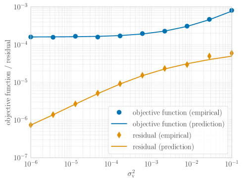
Figure 1: Objective function and residual for the optimizer ($N=100$, $M=90$, $p_{0}=0.8$, $\lambda=0.001$, $p_{\text{X}}(x)$: Bernoulli-Gaussian distribution).

The distribution of the unknown vector $\bm{x}$ is Bernoulli-Gaussian in (9) with $p_{0}=0.8$. In the figure, ‘empirical’ means the empirical value of the objective function $\frac{1}{N}\left(\frac{1}{2}\left\lVert\bm{y}-\bm{A}\hat{\bm{x}}(\lambda)\right\rVert_{2}^{2}+\lambda f\left(\hat{\bm{x}}(\lambda)\right)\right)$ and the residual $\frac{1}{N}\left\lVert\bm{y}-\bm{A}\hat{\bm{x}}(\lambda)\right\rVert_{2}^{2}$, where $\hat{\bm{x}}(\lambda)$ is obtained by the $\ell_{1}$ optimization in (2) with $\lambda=0.001$. The empirical results are averaged over $100$ independent trials. For the reconstruction, we use the LASSO solver of scikit-learn [57]. In Fig. 1, we also plot the asymptotic value obtained from Theorem IV.1 as ‘prediction’. We can see that the empirical value agrees well with the theoretical prediction for both the objective function and the residual.

V Proposed Noise Variance Estimation

In this section, we propose an algorithm for the estimation of the noise variance $\sigma_{\text{v}}^{2}$ on the basis of the asymptotic analysis in Section IV.

V-A Asymptotic Residual Matching

The proposed method uses the fact that the residual $\mathrm{Res}\left(\hat{\bm{x}}(\lambda)\right)\coloneqq\frac{1}{N}\left\lVert\bm{y}-\bm{A}\hat{\bm{x}}(\lambda)\right\rVert_{2}^{2}$ can be approximated by $\left(\beta^{\ast}\right)^{2}$ from (8) when $N$ and $M$ are sufficiently large. Since the function $F(\alpha,\beta)$ to be optimized depends on the regularization parameter $\lambda$, the noise variance $\sigma_{\text{v}}^{2}$, and the sparsity $p_{0}$, the value of the optimal $\beta^{\ast}$ can be considered as a function of $(\lambda,\sigma_{\text{v}}^{2},p_{0})$. To explicitly show the dependency, we denote $\beta^{\ast}$ as $\beta^{\ast}(\lambda,\sigma_{\text{v}}^{2},p_{0})$ hereafter. On the other hand, we can calculate the empirical estimate $\hat{\bm{x}}(\lambda)$ and the corresponding residual $\mathrm{Res}\left(\hat{\bm{x}}(\lambda)\right)$ from (2) without using $\sigma_{\text{v}}^{2}$ in the reconstruction. We can thus estimate the noise variance by choosing $\sigma^{2}$ which minimizes the difference $\left\lvert\beta^{\ast}(\lambda,\sigma^{2},\hat{p}_{0})^{2}-\mathrm{Res}\left(\hat{\bm{x}}(\lambda)\right)\right\rvert$, where $\hat{p}_{0}$ is the estimate of the sparsity $p_{0}$. Hence, the proposed estimate of the noise variance is given by

$$\hat{\sigma}_{\text{v}}^{2} =\operatornamewithlimits{\mathrm{arg\ min}}_{\sigma^{2}>0}\ \left\lvert\beta^{\ast}(\lambda,\sigma^{2},\hat{p}_{0})^{2}-\mathrm{Res}\left(\hat{\bm{x}}(\lambda)\right)\right\rvert.$$ (11)

In the proposed optimization problem (11), we need the estimate of the sparsity $p_{0}$ when $p_{0}$ is unknown. In this paper, we use the simple estimate given by $\hat{p}_{0}=1-\left\lVert\bm{y}\right\rVert_{2}^{2}/M$ on the basis of [58, Eq. (10)]. For simplicity, we here assume that the second moment of the non-zero value of $X\sim p_{\text{X}}$ is $1$ as in (9) and (10). The problem in (11) is a scalar optimization problem over $\sigma^{2}$, and hence the optimal value can be obtained by line search methods such as the ternary search and the golden-section search [56].

Remark V.1 (Advantage of Using Residual of $\ell_{1}$ Optimization).

The proposed estimation method uses the asymptotic result for the residual of the $\ell_{1}$ optimization problem. Although we can use the asymptotic value of the objective function in (7) for the noise variance estimation, the performance would be worse in that case. This is because the line of the objective function is flat especially when the noise variance $\sigma_{\text{v}}^{2}$ is small as shown in Fig. 1. The conventional SNR estimation method in [47] has the same problem because it utilizes the asymptotic result for the objective function of the ridge regularized least squares. In fact, the simulation results in [47] show that the estimation performance becomes worse when the linear system is underdetermined. Another reason for the performance degradation is that the reconstruction performance of the ridge regularized least squares severely degrades for underdetermined problems like compressed sensing. On the other hand, as shown in Fig. 1, the residual of the $\ell_{1}$ optimization decreases more rapidly than the objective function as the noise variance $\sigma_{\text{v}}^{2}$ decreases. We thus conclude that we should use not the objective function but the residual for the noise variance estimation.

V-B Initializaiton of $\lambda$

Since the prediction of the residual from Theorem IV.1 is not exactly accurate for finite $N$, the estimation performance of the proposed optimization problem (11) depends on the parameter $\lambda$. Figure 2 shows the asymptotic residual $\beta^{\ast}(\lambda,\sigma^{2},p_{0})^{2}$ for different values of $\lambda$ when $\Delta=0.8$ and $p_{0}=0.9$.

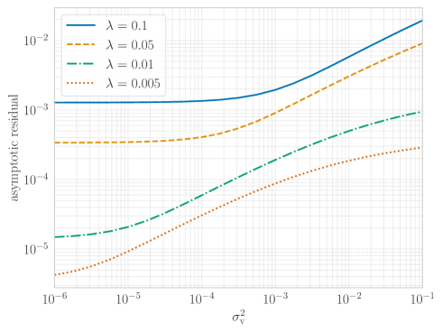
Figure 2: Asymptotic residual of the $\ell_{1}$ optimization ($\Delta=0.8$, $p_{0}=0.9$).

From the figure, we can see that the slope of the line depends on $\lambda$. In the case of Fig. 2, it is difficult to distinguish the noise variance between $10^{-6}$ and $10^{-4}$ if we use the regularization parameter $\lambda=0.1$ because the line of the asymptotic residual with $\lambda=0.1$ is flat in the range. Moreover, if the empirical value of the residual is smaller than the line unfortunately, there might be no positive candidate of $\sigma_{\text{v}}^{2}$. From the above discussion, it would be better to use $\lambda=0.005$ when the true noise variance $\sigma_{\text{v}}^{2}$ is small. On the other hand, when $\sigma_{\text{v}}^{2}=10^{-1}$, for example, the choice $\lambda=0.1$ seems the best of the four in Fig. 2 because it has the steepest slope around $\sigma_{\text{v}}^{2}=10^{-1}$. We need to choose an appropriate value of $\lambda$ to achieve better estimation performance.

To tackle this problem, we propose an initialization method based on the max-min approach. We define the quantity

$$D(\lambda,\sigma^{2},\hat{p}_{0})=\frac{\beta^{\ast}\left(\lambda,(1+\varepsilon)\sigma^{2},\hat{p}_{0}\right)^{2}}{\beta^{\ast}\left(\lambda,\sigma^{2},\hat{p}_{0}\right)^{2}},$$ (12)

which represents how much $\beta^{\ast}$ increases when the value of $\sigma^{2}$ increases to $(1+\varepsilon)\sigma^{2}$ ($\varepsilon>0$). Since the scale of $\beta^{\ast}$ is quite different for different $\lambda$ and $\sigma^{2}$ as shown in Fig. 2, we take the ratio of $\beta^{\ast}\left(\lambda,(1+\varepsilon)\sigma^{2},\hat{p}_{0}\right)^{2}$ to $\beta^{\ast}\left(\lambda,\sigma^{2},\hat{p}_{0}\right)^{2}$. The larger $D(\lambda,\sigma^{2},\hat{p}_{0})$ is, the more rapidly $\left(\beta^{\ast}\right)^{2}$ increases along with the increase of $\sigma^{2}$. Hence, from the discussion of the previous paragraph, $\lambda$ should be chosen so that $D(\lambda,\sigma^{2})$ becomes large. Since the noise variance $\sigma^{2}$ is unknown of course, we here adopt the max-min approach to obtain the proper regularization parameter as

$$\lambda_{\mathrm{prop}}(\hat{p}_{0}) =\operatornamewithlimits{\mathrm{arg\ max}}_{\hskip 5.69054pt0\leq\lambda\leq\lambda_{\mathrm{max}}}\left\{\min_{\sigma^{2}\in\Sigma}D(\lambda,\sigma^{2},\hat{p}_{0})\right\},$$ (13)

where $\lambda_{\mathrm{max}}$ restricts the range of $\lambda$ and $\Sigma$ denotes the set of the candidate values for the noise variance, e.g., $\Sigma=\left\{10^{-5},10^{-3},10^{-1}\right\}$. Note that we does not require that the true noise variance $\sigma_{\text{v}}^{2}$ is included in $\Sigma$. From (13), we can choose a reasonable regularization parameter $\lambda$ in the sense that it maximizes $D(\lambda,\sigma^{2},\hat{p}_{0})$ for the worst $\sigma^{2}\in\Sigma$, without the empirical reconstruction of $\bm{x}$.

V-C Iterative Estimation

To improve the performance, we also propose an iterative approach as in Algorithm 1. We firstly compute the initial regularization parameter $\lambda_{0}=\lambda_{\mathrm{prop}}(\hat{p}_{0})$ with (13), and then iterate the updates of the estimated noise variance $\hat{\sigma}_{\text{v},t}^{2}$ and the regularization parameter $\lambda_{t}$, where $t$ denotes the iteration index. At the $t$-th iteration, the estimate of the noise variance $\hat{\sigma}_{\text{v},t}^{2}$ is calculated by solving (11) with $\lambda=\lambda_{t-1}$. Using the estimate $\hat{\sigma}_{\text{v},t}^{2}$, we update the regularization parameter as

$$\lambda_{t} =\operatornamewithlimits{\mathrm{arg\ max}}_{\hskip 5.69054pt0\leq\lambda\leq\lambda_{\mathrm{max}}}D(\lambda,\hat{\sigma}_{\text{v},t}^{2},\hat{p}_{0}).$$ (14)

to obatin a good regularization parameter for $\hat{\sigma}_{\text{v},t}^{2}$. If the estimate $\hat{\sigma}_{\text{v},t}^{2}$ is closer to the true value $\sigma_{\text{v}}^{2}$ than $\hat{\sigma}_{\text{v},t-1}^{2}$, the new parameter $\lambda_{t}$ is expected to be better than the preivious parameter $\lambda_{t-1}$. After $T$ iterations, the proposed ARM in Algorithm 1 outputs the final estimate of the noise variance $\hat{\sigma}_{\text{v},T}^{2}$.

Algorithm 1 Proposed Asymptotic Residual Matching (ARM)

1:measurement vector $\bm{y}$, measurement matrix $\bm{A}$, estimated sparsity $\hat{p}_{0}$

2:estimated noise variance $\hat{\sigma}_{\text{v},T}^{2}$

3:${\displaystyle\lambda_{0}=\operatornamewithlimits{\mathrm{arg\ max}}_{\hskip 5.69054pt0\leq\lambda\leq\lambda_{\mathrm{max}}}\left\{\min_{\sigma^{2}\in\Sigma}D(\lambda,\sigma^{2},\hat{p}_{0})\right\}}$

4:for $t=1$ to $T$ do

5:     Solve (2) with $\lambda=\lambda_{t-1}$ and obtain $\hat{\bm{x}}(\lambda_{t-1})$.

6:     ${\displaystyle\mathrm{Res}\left(\hat{\bm{x}}(\lambda_{t-1})\right)=\frac{1}{N}\left\lVert\bm{y}-\bm{A}\hat{\bm{x}}(\lambda_{t-1})\right\rVert_{2}^{2}}$

7:     ${\displaystyle\hat{\sigma}_{\text{v},t}^{2}=\operatornamewithlimits{\mathrm{arg\ min}}_{\sigma^{2}>0}\ \left\lvert\beta^{\ast}\left(\lambda_{t-1},\sigma^{2},\hat{p}_{0}\right)^{2}-\mathrm{Res}(\lambda_{t-1})\right\rvert}$

8:     ${\displaystyle\lambda_{t}=\operatornamewithlimits{\mathrm{arg\ max}}_{\hskip 5.69054pt0\leq\lambda\leq\lambda_{\mathrm{max}}}D\left(\lambda,\hat{\sigma}_{\text{v},t}^{2},\hat{p}_{0}\right)}$

9:end for

VI Extension to Other Structured Vectors

Although we have focused on the reconstruction of the sparse vector in the previous sections, the proposed approach using the asymptotic residual can also be applied to the reconstruction of other structured vectors. For example, the noise variance estimation with the proposed ARM approach can be utilized in the reconstruction of discrete-valued vectors because the CGMT-based analysis has been applied to the problem [59, 60]. In this section, we mainly describe the noise variance estimation for the binary vector reconstruction as the simplest example.

In the binary vector reconstruction, we estimate the unknown binary vector $\bm{x}_{\text{b}}\in\left\{1,-1\right\}^{N}$ from its linear measurements $\bm{y}_{\text{b}}=\bm{A}\bm{x}_{\text{b}}+\bm{v}\in\mathbb{R}^{M}$. In this seciton, we consider the unknown vector $\bm{x}_{\text{b}}$ with the distribution

$$p_{\text{X},\text{b}}(x) =\frac{1}{2}\delta_{0}(x+1)+\frac{1}{2}\delta_{0}(x-1).$$ (15)

Such problem often appears in several communication systems, such as the MIMO signal detection [43, 44] and the multiuser detection [61]. As in the sparse vector reconstruction discussed in the previous sections, we require the informarion of the noise variance to obtain better performance with various methods [62, 63, 12, 13] for the binary vector reconstruction.

A simple approach for the binary vector reconstruction is the box relaxation method [64, 65, 59], which solves the optimization problem

$$\hat{\bm{x}}_{\text{b}} =\operatornamewithlimits{\mathrm{arg\ min}}_{\bm{s}\in\left[-1,1\right]^{N}}\left\{\frac{1}{2}\left\lVert\bm{y}_{\text{b}}-\bm{A}\bm{s}\right\rVert_{2}^{2}\right\}.$$ (16)

Using the indicator function

$$f_{\text{b}}(\bm{s}) =\begin{cases}0&(\bm{s}\in\left[-1,1\right]^{N})\\ \infty&(\bm{s}\notin\left[-1,1\right]^{N})\end{cases},$$ (17)

we can rewrite the box relaxation problem in (16) as

$$\hat{\bm{x}}_{\text{b}} =\operatornamewithlimits{\mathrm{arg\ min}}_{\bm{s}\in\mathbb{R}^{N}}\left\{\frac{1}{2}\left\lVert\bm{y}-\bm{A}\bm{s}\right\rVert_{2}^{2}+f_{\text{b}}(\bm{s})\right\}.$$ (18)

The asymptotic analysis in Theorem IV.1 can be applied to the optimization problem in (18). The following corollary shows the result of the analysis, which can be proven in the same way as Theorem IV.1.

Corollary VI.1.

We assume that Assumption IV.1 is satisfied. We also assume that the optimization problem $\min_{\alpha>0}\max_{\beta\geq 0}F_{\text{b}}(\alpha,\beta)$ has a unique optimizer $(\alpha_{\text{b}}^{\ast},\beta_{\text{b}}^{\ast})$, where

$$F_{\text{b}}(\alpha,\beta) =\frac{\alpha\beta\sqrt{\Delta}}{2}+\frac{\sigma_{\text{v}}^{2}\beta\sqrt{\Delta}}{2\alpha}-\frac{1}{2}\beta^{2}-\frac{\alpha\beta}{2\sqrt{\Delta}}$$

$$\hskip 11.38109pt+\frac{\beta\sqrt{\Delta}}{\alpha}\mathrm{E}\left[\mathrm{env}_{\frac{\alpha}{\beta\sqrt{\Delta}}f_{\text{b}}}\left(X_{\text{b}}+\frac{\alpha}{\sqrt{\Delta}}G\right)\right]$$ (19)

and $X_{\text{b}}\sim p_{\text{X},\text{b}},G\sim p_{\text{G}}$. Then, the asymptotic value of the objective function in (16) and the residual for the optimizer $\hat{\bm{x}}_{\text{b}}$ are given by

$$\operatornamewithlimits{\mathrm{plim}}_{N\to\infty}\ \frac{1}{N}\left(\frac{1}{2}\left\lVert\bm{y}-\bm{A}\hat{\bm{x}}_{\text{b}}\right\rVert_{2}^{2}\right)=F_{\text{b}}\left(\alpha_{\text{b}}^{\ast},\beta_{\text{b}}^{\ast}\right),$$ (20)

$$\operatornamewithlimits{\mathrm{plim}}_{N\to\infty}\ \frac{1}{N}\left\lVert\bm{y}_{\text{b}}-\bm{A}\hat{\bm{x}}_{\text{b}}\right\rVert_{2}^{2}=(\beta_{\text{b}}^{\ast})^{2},$$ (21)

respectively.

Thus, we can estimate the noise variance in the binary vector reconstruction by using the proposed ARM. It should be noted that we do not require the tuning of the regularization parameter in this case because the optimization problem in (16) does not contain any regularization parameter. Hence, the estimate of the noise variance can be obtained by the non-iterative approach as shown in Algorithm 2. Note that the information of the noise variance is useful for other reconstruction methods such as [62, 63, 12, 13], though the box relaxation does not include any parameter to be tuned.

Algorithm 2 Proposed ARM for binary vector reconstruction

1:measurement vector $\bm{y}_{\text{b}}$, measurement matrix $\bm{A}$

2:estimated noise variance $\hat{\sigma}_{\text{v}}^{2}$

3:Solve (16) and obtain $\hat{\bm{x}}_{\text{b}}$.

4:${\displaystyle\mathrm{Res}(\hat{\bm{x}}_{\text{b}})=\frac{1}{N}\left\lVert\bm{y}_{\text{b}}-\bm{A}\hat{\bm{x}}_{\text{b}}\right\rVert_{2}^{2}}$

5:${\displaystyle\hat{\sigma}_{\text{v}}^{2}=\operatornamewithlimits{\mathrm{arg\ min}}_{\sigma^{2}>0}\ \left\lvert\beta_{\text{b}}^{\ast}\left(\sigma^{2}\right)^{2}-\mathrm{Res}(\hat{\bm{x}}_{\text{b}})\right\rvert}$

The proposed ARM can also be applied to the binary sparse vector reconstruction and more general discrete-valued vector reconstruction [10, 55, 60] by using Theorem IV.1 with the corresponding distribution $p_{X}$ and the proper regularizer $f(\cdot)$.

VII Simulation Results

In this section, we show some simulation results to demonstrate the performance of the proposed noise variance estimation. In the simulations, we compare the following methods.

• ARM: the noise variance estimation with the proposed ARM in Algorithms 1 or 2. For the optimization of $\sigma^{2}$ in (11) and $\lambda$ in (13), (14), we use the scalar minimization solver scipy.optimize.minimize_scalar of scipy [66]. The set $\Sigma$ in (13) is fixed as $\Sigma=\left\{10^{-5},10^{-3},10^{-1}\right\}$ and $\lambda_{\mathrm{max}}=1$ in the simulations. The value of $\varepsilon$ in (12) is set as $\varepsilon=0.1$.

• AMP-LASSO: the estimation method using AMP-LASSO given by (4) [39]. Since the tuning of the regularization parameter for AMP-LASSO have not been discussed in the paper, we use the proposed value $\lambda_{\mathrm{prop}}(\hat{p}_{0})$ unless otherwise stated.

• scaled residual: the estimation method using the scaled residual given by (3).

• ridge regularization-based method: the conventional SNR estimation method in [47] based on the asymptotic analysis of ridge regularized least squares. The regularization parameters are the same as those in [47].

• ML (oracle): the maximum likelihood (ML) approach when the true sparse vector $\bm{x}$ is known. The estimate of $\sigma_{\text{v}}^{2}$ is given by $\hat{\sigma}_{\text{v}}^{2}=\frac{1}{M}\left\lVert\bm{y}-\bm{A}\bm{x}\right\rVert_{2}^{2}$. Note that $\bm{x}$ is unknown in the other methods.

In all methods, the noise variance is estimated in the range $[10^{-6},1]$. The measurement matrix $\bm{A}$ and the noise vector $\bm{v}$ satisfy Assumption IV.1 in the simulations.

VII-A Sparse Vector Reconstruction

We firstly examine the effect of the regularization parameter $\lambda$ in the noise variance estimation for the sparse vector reconstruction. Figure 3 shows the estimate of the noise variance $\hat{\sigma}_{\text{v}}^{2}$ versus the regularization parameter $\lambda$ for $N=200$ and $\Delta=0.7$.

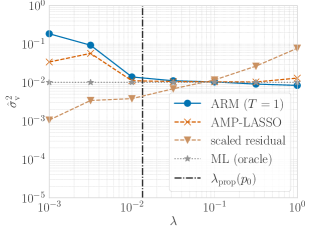
(a) $\sigma_{\text{v}}^{2}=0.01$

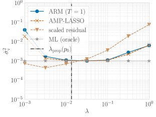
(b) $\sigma_{\text{v}}^{2}=0.001$

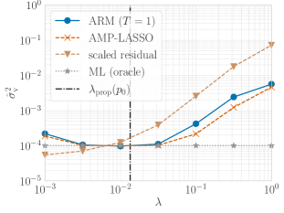
(c) $\sigma_{\text{v}}^{2}=0.0001$

Figure 3: Estimated $\hat{\sigma}_{\text{v}}^{2}$ versus $\lambda$ ($N=200,\Delta=0.7,p_{0}=0.9$, $p_{\text{X}}(x)$: Bernoulli-Gaussian distribution).

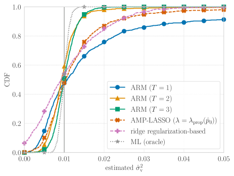
(a) $\sigma_{\text{v}}^{2}=0.01$

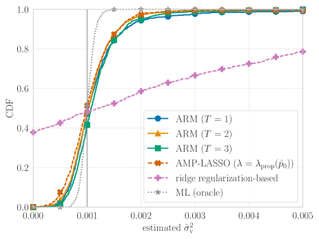
(b) $\sigma_{\text{v}}^{2}=0.001$

Figure 4: CDF of estimated $\hat{\sigma}_{\text{v}}^{2}$ ($N=200$, $\Delta=0.6$, $p_{0}=0.9$, $p_{\text{X}}(x)$: Bernoulli-Gaussian distribution).

The distribution of the unknown vector is the Bernoulli-Gaussian distribution in (9) with $p_{0}=0.9$. The true noise variance is set as $\sigma_{\text{v}}^{2}=0.01,0.001$, and $0.0001$ in Figs. 3, 3 and 3, respectively. To solve (2) in ARM, AMP-LASSO, and scaled residual, we use the LASSO solver of scikit-learn [57]. The estimated value is averaged over $100$ independent trials. In the figures, the black vertical line shows the value of the proposed regularization parameter $\lambda_{\mathrm{prop}}(p_{0})$ with the true probability $p_{0}$. Although the estimation performance depends on $\lambda$, the proposed regularization parameter can achieve good performance in both ARM and AMP-LASSO for $\sigma_{\text{v}}^{2}=0.01,0.001$, and $0.0001$. We can also see that the performance of the scaled residual is worse than the other methods.

Figure 4 shows the histogram of the empirical CDF of the estimated $\hat{\sigma}_{\text{v}}^{2}$, where $N=200$, $\Delta=0.6$, and $p_{0}=0.9$. The histogram is obtained from $1000$ independent trials. Since the true noise variance is set to $\sigma_{\text{v}}^{2}=0.01$ in Fig. 4, it is better that the CDF rapidly increases around $\sigma_{\text{v}}^{2}=0.01$. From the figure, we can see that the CDF of the proposed ARM with $T=3$ increases around $\sigma_{\text{v}}^{2}=0.01$ more rapidly than AMP-LASSO and the ridge regularization-based method. This means that the proposed method obtains the estimate near the true value with a higher probability. The figure also shows that the performance of the proposed ARM improves as the number of iterations $T$ increases. Figure 4 shows the performance for $\sigma_{\text{v}}^{2}=0.001$, where the proposed ARM and AMP-LASSO achieves similar performance. However, it should be noted that we use the proposed regularization parameter $\lambda_{\mathrm{prop}}(\hat{p}_{0})$ for AMP-LASSO. The performance of AMP-LASSO degrades if we use an inappropriate parameter value as shown in Fig. 3. We can see that the proposed ARM with $T=2,3$ achieves the similar performance for both $\sigma_{\text{v}}^{2}=0.01$ and $\sigma_{\text{v}}^{2}=0.001$, whereas the performance of AMP-LASSO and the ridge regularization-based method largely depends on the true value of $\sigma_{\text{v}}^{2}$.

We then evaluate the estimation performance for a wide range of the noise variance. In Fig. 5, we plot the estimate $\hat{\sigma}_{\text{v}}^{2}$ versus its true value $\sigma_{\text{v}}^{2}$ when $N=200$, $\Delta=0.6$, and $p_{0}=0.9$.

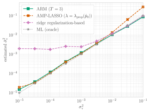
Figure 5: Estimated $\hat{\sigma}_{\text{v}}^{2}$ versus $\sigma_{\text{v}}^{2}$ ($N=200$, $\Delta=0.6$, $p_{0}=0.9$, $p_{\text{X}}(x)$: Bernoulli-Gaussian distribution).

The performance is obtained by averaging the result of $100$ independent trials. The figure shows that the proposed ARM with $T=3$ can achieve good estimation performance close to ‘ML (oracle)’ for the whole range of $\sigma_{\text{v}}^{2}$ in the figure. On the other hand, the performance of AMP-LASSO and the ridge regularization-based method degrades for the large $\sigma_{\text{v}}^{2}$ and small $\sigma_{\text{v}}^{2}$, respectively.

Next, we demonstrate the reconstruction performance of the optimization problem in (2) with the proposed noise variance estimation. Figure 6 shows the CDF of the MSE $\frac{1}{N}\left\lVert\hat{\bm{x}}-\bm{x}\right\rVert_{2}^{2}$ ($\hat{\bm{x}}$: estimate of $\bm{x}$) obteind with $1000$ independent trials, where $\Delta=0.7$, $p_{0}=0.8$, and $\sigma_{\text{v}}^{2}=0.001$.

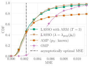
(a) $N=100$

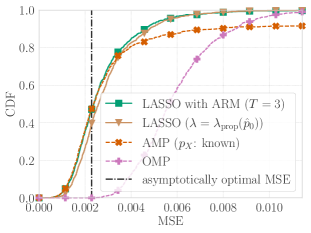
(b) $N=200$

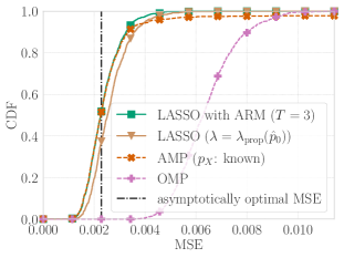
(c) $N=500$

Figure 6: CDF of MSE ($\Delta=0.7$, $p_{0}=0.8$, $\sigma_{\text{v}}^{2}=0.001$, $p_{\text{X}}(x)$: Bernoulli-Gaussian distribution).

The dimension of the unknown vector is set as $N=100$, $200$, and $500$ in Figs. 6, 6, and 6, respectively. In the figures, ‘LASSO with ARM’ shows the performance of the optimization problem (2) with the parameter tuning by the proposed ARM. Specifically, we firstly obtain the estimate of the noise variance $\hat{\sigma}_{\text{v}}^{2}$ with the proposed ARM, and then calculate the optimal value of $\lambda$ in terms of asymptotic MSE by using the estimated $\hat{\sigma}_{\text{v}}^{2}$ and $\hat{p}_{0}$ via the CGMT framework. For comparison, we also plot the performance of LASSO with the proposed initial regularization parameter $\lambda=\lambda_{\mathrm{prop}}(\hat{p}_{0})$ in (13) as ‘LASSO ($\lambda=\lambda_{\mathrm{prop}}(\hat{p}_{0})$)’. Moreover, we show the performance of the AMP algorithm with the optimal thresholding parameters [41] as ‘AMP’, for which the distribution of the unknown vector $p_{X}$ is assumed to be perfectly known. In addition, ‘OMP’ denotes the performance of the OMP algorithm with the tolerance of $10^{-3}$, which is implemented by using the solver of scikit-learn. In the figure, the vertical black line shows the asymptotically optimal MSE, which can be obtained by the CGMT or AMP framework. From the figure, we can see that LASSO outperforms the other methods especially when $N$ is small. On the other hand, the CDF of the AMP algorithm is far from one when $N=100$ and $N=200$, which means that the AMP algorithm results in a large MSE or even diverges. This is because the large system limit is usually assumed in the AMP framework to obtain the low-complexity algorithm and the insightful analysis. Since the AMP algorithm achieves a similar performance to LASSO when $N=500$, it would be a suitable candidate for large-scale problems. The performance of the OMP algorithm is worse than the other methods, and hence somehow we need to choose an appropriate tolerance parameter. These results show that the proposed noise variance estimation enables us to obtain good reconstruction performance even when the true noise variance is unknown and the problem size is relatively small.

Figure 7 shows the CDF of the MSE obteind with $1000$ independent trials, where $\Delta=0.7$, $p_{0}=0.8$, and $\sigma_{\text{v}}^{2}=0.005$.

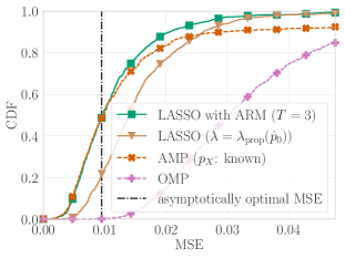
(a) $N=100$

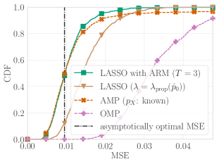
(b) $N=200$

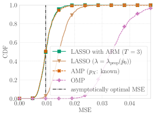
(c) $N=500$

Figure 7: CDF of MSE ($\Delta=0.7$, $p_{0}=0.8$, $\sigma_{\text{v}}^{2}=0.005$, $p_{\text{X}}(x)$: Bernoulli-Gaussian distribution).

We obsereve that the performance of LASSO with $\lambda=\lambda_{\mathrm{prop}}(\hat{p}_{0})$ degrades compared to the case with Fig. 6. On the other hand, LASSO with ARM can achieve good performance even in this case, which shows the effectiveness of the noise variance estimation for the parameter tuning.

VII-B Binary Vector Reconstruction

We then investigate the performance when the unknown vector is a binary vector with the distribution in (15). Figure 8 shows the histogram of the empirical CDF of the estimated $\hat{\sigma}_{\text{v}}^{2}$ when $N=200$, $\Delta=0.8$, and $\sigma_{\text{v}}^{2}=0.01$.

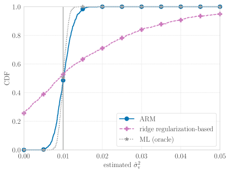
Figure 8: CDF of estimated $\hat{\sigma}_{\text{v}}^{2}$ ($N=200$, $\Delta=0.8$, $\sigma_{\text{v}}^{2}=0.01$, $p_{\text{X},\text{b}}(x)$: Binary distribution).

In the simulation, we use ADMM [25, 26, 27, 28] to solve the optimization problem (16). Since the estimate by AMP-LASSO in (4) cannot be directly applied to the binary vector reconstruction, we compare the performance of the proposed method with the ridge-regularization based method [47]. As is the case with the Bernoulli-Gaussian distribution in Fig. 4, the proposed ARM in Algorithm 2 achieves better performance than the ridge regularization-based method.

Finally, we evaluate the estimation performance versus the true noise variance $\sigma_{\text{v}}^{2}$. Figure 9 shows the performance when $N=200$ and $\Delta=0.7$.

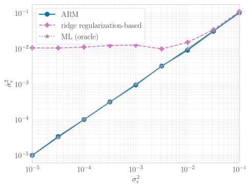
Figure 9: Estimated $\hat{\sigma}_{\text{v}}^{2}$ versus $\sigma_{\text{v}}^{2}$ ($N=200$, $\Delta=0.7$, $p_{\text{X},\text{b}}(x)$: Binary distribution).

The performance is obtained by averaging the result of $100$ independent trials. We observe that the proposed method achieves good estimation performance for a wide range of the noise variance as is the case with Fig. 5. We thus conclude that the proposed noise variance estimation is effective for the binary distribution $p_{\text{X},\text{b}}(x)$.

VIII Conclusion

In this paper, we have proposed the noise variance estimation algorithm for compressed sensing with the Gaussian measurement matrix. The proposed ARM algorithm utilizes the asymptotic property of the estimate obtained by the $\ell_{1}$ optimization problem. Specifically, we estimate the noise variance by choosing the value whose corresponding asymptotic residual matches the empirical residual obtained by the actual reconstruction. The main advantages of the proposed approach can be summarized as follows:

• The proposed method can estimate a wide range of the noise variance even in the underdetermined problems.

• We can design the choice of the regularization parameter $\lambda$ on the basis of the asymptotic results.

• The proposed idea using the asymptotic residual can be extended for the reconstruction of some structured vectors other than sparse ones as shown in Section VI.

• The proposed methods can achieve good performance even when the problem size is relatively small.

Simulation results demonstrate that the proposed method can achieve better estimation performance than some conventional methods. Moreover, by using the estimate of the noise variance, we can choose an appropriate regularization parameter even when the noise variance is unknown. We have shown that the LASSO with the proposed noise variance estimation can achieve better performance than the AMP algorithm for small-scale problems.

Compared to AMP-LASSO in (4) and the scaled residual method in (3), the procedure of the proposed ARM is slightly complicated. For example, we need to estimate the sparsity of the unknown vector and solve some scalar optimization problems in the estimation. It would be an interesting research direction to apply the proposed idea for the choice of the regularization parameter $\lambda$ to the AMP-based methods. Although we have focused on the compressed sensing problem from the perspective of signal processing in this paper, the application of the proposed approach to statistics would also be a fascinating topic.

It would be possible to apply the idea of the proposed approach to the case with other structured signals or other optimization problems because CGMT can be used for various optimization problems [67, 33, 59, 68]. Since CGMT has also been applied to an optimization problem in the complex-valued domain [69], the extension to the complex-valued case could also be an interesting research direction.

Appendix A Proof of Theorem IV.1

In this section, we give the proof of Theorem IV.1. Although the procedure of the proof partly follows some CGMT-based analyses (e.g., [33, 59, 60]), we here show the sketch of the proof to derive the explicit formula in Theorem IV.1.

A-A CGMT

We firstly summarize CGMT [42, 33] before the proof of Theorem IV.1. CGMT associates the following primary optimization (PO) and auxiliary optimization (AO).

$$(\text{PO}):\ \Phi(\bm{G})=\min_{\bm{w}\in\mathcal{S}_{\text{w}}}\max_{\bm{u}\in\mathcal{S}_{\text{u}}}\left\{\bm{u}^{\mathsf{T}}\bm{G}\bm{w}+\xi(\bm{w},\bm{u})\right\}$$ (22)

$$(\text{AO}):\ \phi(\bm{g},\bm{h})=\min_{\bm{w}\in\mathcal{S}_{\text{w}}}\max_{\bm{u}\in\mathcal{S}_{\text{u}}}\left\{\left\lVert\bm{w}\right\rVert_{2}\bm{g}^{\mathsf{T}}\bm{u}-\left\lVert\bm{u}\right\rVert_{2}\bm{h}^{\mathsf{T}}\bm{w}\right.$$

$$\hskip 142.26378pt\left.+\ \xi(\bm{w},\bm{u})\right\}$$ (23)

Here, $\bm{G}\in\mathbb{R}^{K\times L}$, $\bm{g}\in\mathbb{R}^{K}$, and $\bm{h}\in\mathbb{R}^{L}$ are composed of i.i.d. standard Gaussian variables. The constraint sets $\mathcal{S}_{\text{w}}\subset\mathbb{R}^{L}$ and $\mathcal{S}_{\text{u}}\subset\mathbb{R}^{K}$ are assumed to be closed compact. The function $\xi(\cdot,\cdot)$ is a continuous convex-concave function on $\mathcal{S}_{\text{w}}\times\mathcal{S}_{\text{u}}$.

As in the following theorem, we can relate the optimal costs $\Phi(\bm{G}),\phi(\bm{g},\bm{h})$ and the optimizer $\hat{\bm{w}}_{\Phi}(\bm{G})$ of (PO) (For more details, see [33, Theorem 3] and [59, Theorem IV.2]).

Theorem A.1 (CGMT).

1. For all $\mu\in\mathbb{R}$ and $c>0$, we have

   $$\Pr(\left\lvert\Phi(\bm{G})-\mu\right\rvert>c)\leq 2\Pr(\left\lvert\phi(\bm{g},\bm{h})-\mu\right\rvert\geq c).$$ (24)

2. Let $\mathcal{S}$ be a open set in $\mathcal{S}_{\text{w}}$ and $\mathcal{S}^{\text{c}}=\mathcal{S}_{\text{w}}\setminus\mathcal{S}$. Moreover, we denote the optimal cost of (AO) with the constraint $\bm{w}\in\mathcal{S}^{\text{c}}$ by $\phi_{\mathcal{S}^{\text{c}}}(\bm{g},\bm{h})$. If there exists constants $\bar{\phi}$ and $\eta$ ($>0$) such that $\phi(\bm{g},\bm{h})\leq\bar{\phi}+\eta$ and $\phi_{\mathcal{S}^{\text{c}}}(\bm{g},\bm{h})\geq\bar{\phi}+2\eta$ with probability approaching $1$ as $L\to\infty$, we then have

   $$\lim_{L\to\infty}\Pr(\hat{\bm{w}}_{\Phi}(\bm{G})\in\mathcal{S})=1,$$ (25)

   where $L\to\infty$ means that $K$ and $L$ go to infinity with a fixed ratio.

A-B (PO) Problem

To obtain the result of Theorem IV.1 by using CGMT, we rewrite the $\ell_{1}$ optimization problem (2) as (PO) problem. We firstly define the error vector $\bm{u}=\bm{s}-\bm{x}$ and rewrite (2) as

$$\Phi_{N}^{\ast}\coloneqq\min_{\bm{u}\in\mathbb{R}^{N}}\frac{1}{N}\left\{\frac{1}{2}\left\lVert\bm{A}\bm{u}-\bm{v}\right\rVert_{2}^{2}+\lambda f(\bm{x}+\bm{u})\right\},$$ (26)

where the objective function is normalized by $N$. From [33, Lemma 5], we can introduce a compact set $\mathcal{S}_{\text{u}}\coloneqq\left\{\bm{u}\mid\left\lVert\bm{u}\right\rVert_{2}\leq C_{\text{u}}\right\}$ with a constant $C_{\text{u}}$ ($>0$) as

$$\Phi_{N}^{\ast}=\min_{\bm{u}\in\mathcal{S}_{\text{u}}}\frac{1}{N}\left\{\frac{1}{2}\left\lVert\bm{A}\bm{u}-\bm{v}\right\rVert_{2}^{2}+\lambda f(\bm{x}+\bm{u})\right\}.$$ (27)

Since we have

$$\frac{1}{2}\left\lVert\bm{A}\bm{u}-\bm{v}\right\rVert_{2}^{2} =\max_{\bm{w}\in\mathbb{R}^{M}}\left\{\sqrt{N}\bm{w}^{\mathsf{T}}(\bm{A}\bm{u}-\bm{v})-\frac{N}{2}\left\lVert\bm{w}\right\rVert_{2}^{2}\right\},$$ (28)

the optimization problem can be represented as

$$\Phi_{N}^{\ast} =\min_{\bm{u}\in\mathcal{S}_{\text{u}}}\max_{\bm{w}\in\mathbb{R}^{M}}\Biggl{\{}\frac{1}{N}\bm{w}^{\mathsf{T}}\left(\sqrt{N}\bm{A}\right)\bm{u}-\frac{1}{\sqrt{N}}\bm{v}^{\mathsf{T}}\bm{w}$$

$$\hskip 85.35826pt-\frac{1}{2}\left\lVert\bm{w}\right\rVert_{2}^{2}+\frac{\lambda}{N}f(\bm{x}+\bm{u})\Biggr{\}}.$$ (29)

Moreover, by using [33, Lemma 6], we can introduce a sufficiently large constraint set $\mathcal{S}_{\text{w}}\coloneqq\left\{\bm{w}\mid\left\lVert\bm{w}\right\rVert_{2}\leq C_{\text{w}}\right\}\ (C_{\text{w}}>0)$ which will not affect the optimization problem with high probability as

$$\Phi_{N}^{\ast} =\min_{\bm{u}\in\mathcal{S}_{\text{u}}}\max_{\bm{w}\in\mathcal{S}_{\text{w}}}\Biggl{\{}\frac{1}{N}\bm{w}^{\mathsf{T}}\left(\sqrt{N}\bm{A}\right)\bm{u}-\frac{1}{\sqrt{N}}\bm{v}^{\mathsf{T}}\bm{w}$$

$$\hskip 85.35826pt-\frac{1}{2}\left\lVert\bm{w}\right\rVert_{2}^{2}+\frac{\lambda}{N}f(\bm{x}+\bm{u})\Biggr{\}}.$$ (30)

In the standard analysis based on CGMT, the minimization problem for the error vector $\bm{u}$ is analyzed. In our proof, however, we analyze the optimal value of $\bm{w}$ to obtain the result for the residual. We thus exchange the order of min-max from the minimax theorem and change the sign of the objective function to obtain

$$-\Phi_{N}^{\ast} =\min_{\bm{w}\in\mathcal{S}_{\text{w}}}\max_{\bm{u}\in\mathcal{S}_{\text{u}}}\Biggl{\{}\frac{1}{N}\bm{w}^{\mathsf{T}}\left(\sqrt{N}\bm{A}\right)\bm{u}+\frac{1}{\sqrt{N}}\bm{v}^{\mathsf{T}}\bm{w}$$

$$\hskip 85.35826pt+\frac{1}{2}\left\lVert\bm{w}\right\rVert_{2}^{2}-\frac{\lambda}{N}f(\bm{x}+\bm{u})\Biggr{\}},$$ (31)

where we can keep the sign of the first term $\frac{1}{N}\bm{w}^{\mathsf{T}}(\sqrt{N}\bm{A})\bm{u}$ because the distribution of the matrix $\bm{A}$ is zero mean Gaussian and sign independent. The optimization problem (31) is the form of (PO) normalized by $N$. Note that the optimal value of $\bm{w}$ can be written as

$$\hat{\bm{w}}_{N}^{(\text{PO})} =\frac{1}{\sqrt{N}}\left(\bm{A}\hat{\bm{u}}_{N}^{(\text{PO})}-\bm{v}\right)$$ (32)

$$=\frac{1}{\sqrt{N}}\left(\bm{A}\hat{\bm{x}}(\lambda)-\bm{y}\right)$$ (33)

from (28), where $\hat{\bm{u}}_{N}^{(\text{PO})}=\hat{\bm{x}}(\lambda)-\bm{x}$ is the optimal value of $\bm{u}$ in (PO).

A-C (AO) Problem

We then analyze the corresponding (AO) problem. Since the procedure is similar to [60], we omit some details in the analysis. The (AO) problem corresponding to (31) is given by

$$-\phi_{N}^{\ast} \coloneqq\min_{\bm{w}\in\mathcal{S}_{\text{w}}}\max_{\bm{u}\in\mathcal{S}_{\text{u}}}\Biggl{\{}\frac{1}{N}(\left\lVert\bm{w}\right\rVert_{2}\bm{g}^{\mathsf{T}}\bm{u}-\left\lVert\bm{u}\right\rVert_{2}\bm{h}^{\mathsf{T}}\bm{w})$$

$$\hskip 56.9055pt+\frac{1}{\sqrt{N}}\bm{v}^{\mathsf{T}}\bm{w}+\frac{1}{2}\left\lVert\bm{w}\right\rVert_{2}^{2}-\frac{\lambda}{N}f(\bm{x}+\bm{u})\Biggr{\}}.$$ (34)

Since the objective function in (34) is not convex-concave, the order of min-max cannot be exchanged in general. As described in [33, Appendix A], however, we can flip the order in the asymptotic setting because the corresponding (PO) satisfies the condition for the min-max theorem. Hence, we exchange the order of min-max without detailed explanations hereafter. By exchanging the order of min-max and changing the sign of the objective function, we obtain

$$\phi_{N}^{\ast} =\min_{\bm{u}\in\mathcal{S}_{\text{u}}}\max_{\bm{w}\in\mathcal{S}_{\text{w}}}\Biggl{\{}-\frac{1}{N}(\left\lVert\bm{w}\right\rVert_{2}\bm{g}^{\mathsf{T}}\bm{u}-\left\lVert\bm{u}\right\rVert_{2}\bm{h}^{\mathsf{T}}\bm{w})$$

$$\hskip 56.9055pt-\frac{1}{\sqrt{N}}\bm{v}^{\mathsf{T}}\bm{w}-\frac{1}{2}\left\lVert\bm{w}\right\rVert_{2}^{2}+\frac{\lambda}{N}f(\bm{x}+\bm{u})\Biggr{\}}.$$ (35)

Taking advantage of the fact that both $\bm{h}$ and $\bm{v}$ are Gaussian, we can rewrite $\frac{\left\lVert\bm{u}\right\rVert_{2}}{\sqrt{N}}\bm{h}-\bm{v}$ as $\sqrt{\frac{\left\lVert\bm{u}\right\rVert_{2}^{2}}{N}+\sigma_{\text{v}}^{2}}\ \bm{h}$, where we use the slight abuse of notation $\bm{h}$ as i.i.d. standard Gaussian variables. Using this technique, we can set $\left\lVert\bm{w}\right\rVert_{2}=\beta$ and obtain the equivalent optimization problem

$$\phi_{N}^{\ast} =\min_{\bm{u}\in\mathcal{S}_{\text{u}}}\max_{\beta\geq 0}\Biggl{\{}\sqrt{\frac{\left\lVert\bm{u}\right\rVert_{2}^{2}}{N}+\sigma_{\text{v}}^{2}}\frac{\beta\left\lVert\bm{h}\right\rVert_{2}}{\sqrt{N}}-\frac{1}{N}\beta\bm{g}^{\mathsf{T}}\bm{u}$$

$$\hskip 85.35826pt-\frac{1}{2}\beta^{2}+\frac{\lambda}{N}f(\bm{x}+\bm{u})\Biggr{\}}.$$ (36)

To further rewrite the optimization problem (36), we use the following identity

$$\chi =\min_{\alpha>0}\left(\frac{\alpha}{2}+\frac{\chi^{2}}{2\alpha}\right)$$ (37)

for $\chi=\sqrt{\frac{\left\lVert\bm{u}\right\rVert_{2}^{2}}{N}+\sigma_{\text{v}}^{2}}$ and obtain

$$\min_{\alpha>0}\max_{\beta\geq 0}\Biggl{\{}\frac{\alpha\beta}{2}\frac{\left\lVert\bm{h}\right\rVert_{2}}{\sqrt{N}}+\frac{\sigma_{\text{v}}^{2}\beta}{2\alpha}\frac{\left\lVert\bm{h}\right\rVert_{2}}{\sqrt{N}}-\frac{1}{2}\beta^{2}-\frac{1}{N}\frac{\alpha\beta\left\lVert\bm{g}\right\rVert_{2}^{2}}{2}\frac{\sqrt{N}}{\left\lVert\bm{h}\right\rVert_{2}}$$

$$\hskip 99.58464pt+\frac{\beta}{\alpha}\frac{\left\lVert\bm{h}\right\rVert_{2}}{\sqrt{N}}\frac{1}{N}\sum_{n=1}^{N}\min_{u_{n}\in\mathbb{R}}J_{n}(u_{n})\Biggr{\}},$$ (38)

where we define

$$J_{n}(u_{n}) =\frac{1}{2}\left(u_{n}-\frac{\sqrt{N}}{\left\lVert\bm{h}\right\rVert_{2}}\alpha g_{n}\right)^{2}+\frac{\alpha\lambda}{\beta}\frac{\sqrt{N}}{\left\lVert\bm{h}\right\rVert_{2}}f(x_{n}+u_{n}).$$ (39)

Here, $u_{n}$ and $g_{n}$ are the $n$-th element of $\bm{u}$ and $\bm{g}$, respectively. Since we have

$$\min_{u_{n}\in\mathbb{R}}J_{n}(u_{n}) =\mathrm{env}_{\frac{\alpha\lambda}{\beta}\frac{\sqrt{N}}{\left\lVert\bm{h}\right\rVert_{2}}f}\left(x_{n}+\frac{\sqrt{N}}{\left\lVert\bm{h}\right\rVert_{2}}\alpha g_{n}\right),$$ (40)

the (AO) problem can be written as

$$\phi_{N}^{\ast} =\min_{\alpha>0}\max_{\beta\geq 0}F_{N}(\alpha,\beta),$$ (41)

where

$$F_{N}(\alpha,\beta)$$

$$=\frac{\alpha\beta}{2}\frac{\left\lVert\bm{h}\right\rVert_{2}}{\sqrt{N}}+\frac{\sigma_{\text{v}}^{2}\beta}{2\alpha}\frac{\left\lVert\bm{h}\right\rVert_{2}}{\sqrt{N}}-\frac{1}{2}\beta^{2}-\frac{1}{N}\frac{\alpha\beta\left\lVert\bm{g}\right\rVert_{2}^{2}}{2}\frac{\sqrt{N}}{\left\lVert\bm{h}\right\rVert_{2}}$$

$$\hskip 11.38109pt+\frac{\beta}{\alpha}\frac{\left\lVert\bm{h}\right\rVert_{2}}{\sqrt{N}}\frac{1}{N}\sum_{n=1}^{N}\mathrm{env}_{\frac{\alpha\lambda}{\beta}\frac{\sqrt{N}}{\left\lVert\bm{h}\right\rVert_{2}}f}\left(x_{n}+\frac{\sqrt{N}}{\left\lVert\bm{h}\right\rVert_{2}}\alpha g_{n}\right).$$ (42)

We denote the optimal values of $\alpha$ and $\beta$ in the (AO) problem by $\alpha_{N}^{\ast}$ and $\beta_{N}^{\ast}$, respectively.

A-D Applying CGMT

By using the above analysis, we confirm (7) in Theorem IV.1. As $N\to\infty$, $F_{N}(\alpha,\beta)$ in (42) converges pointwise to $F(\alpha,\beta)$ in (6). Letting $\phi^{\ast}=F(\alpha^{\ast},\beta^{\ast})$ be the optimal value of $F(\alpha,\beta)$, we can obtain $-\phi_{N}^{\ast}\xrightarrow{\mathrm{P}}-\phi^{\ast}$ and $(\alpha_{N}^{\ast},\beta_{N}^{\ast})\xrightarrow{\mathrm{P}}(\alpha^{\ast},\beta^{\ast})$ as $N\to\infty$ by a similar approach to the proof of [59, Lemma IV. 1]. Hence, by setting $\mu=-\phi^{\ast}$ in (24) of Theorem A.1, we have $\lim_{N\to\infty}\Pr(\left\lvert-\Phi_{N}^{\ast}-(-\phi^{\ast})\right\rvert>c)=0$ for any $c>0$, which means (7).

We can also demonstrate the convergence of the residual in (8) from the second statement in Theorem A.1. We denote the optimal value of $\bm{w}$ in (34) by $\hat{\bm{w}}_{N}^{(\text{AO})}$ and define

$$\mathcal{S} =\left\{\bm{z}\in\mathbb{R}^{M}\Bigg{|}\left\lvert\left\lVert\bm{z}\right\rVert_{2}^{2}-\left(\beta^{\ast}\right)^{2}\right\rvert<\varepsilon\right\}.$$ (43)

We then have $\hat{\bm{w}}_{N}^{(\text{AO})}\in\mathcal{S}$ with probability approaching $1$ for any $\varepsilon$ ($>0$) because $\left\lVert\hat{\bm{w}}_{N}^{(\text{AO})}\right\rVert_{2}=\beta_{N}^{\ast}$ from the definition of $\beta$ and $\beta_{N}^{\ast}\xrightarrow{\mathrm{P}}\beta^{\ast}$. Considering the strong concavity of the objective function in (36) over $\beta$, we can see that there exists $\eta$ ($>0$) satisfying the condition in Theorem A.1 with $\bar{\phi}=-\phi^{\ast}$. We thus have $\lim_{N\to\infty}\Pr\left(\hat{\bm{w}}_{N}^{(\text{PO})}\in\mathcal{S}\right)=1$, i.e.,

$$\operatornamewithlimits{\mathrm{plim}}_{N\to\infty}\ \left\lVert\hat{\bm{w}}_{N}^{(\text{PO})}\right\rVert_{2}^{2}=(\beta^{\ast})^{2}.$$ (44)

Combining (33) and (44) concludes the proof.

Appendix B On Expectation in (6)

In this section, we derive the explicit formula of the expectation in (6) for the Bernoulli-Gaussian distribution in (9). The expectation in (6) can be written as

$$\mathrm{E}\left[\mathrm{env}_{\frac{\alpha\lambda}{\beta\sqrt{\Delta}}f}\left(X+\frac{\alpha}{\sqrt{\Delta}}G\right)\right]$$

$$=\frac{\alpha\lambda}{\beta\sqrt{\Delta}}\mathrm{E}\left[f\left(\mathrm{prox}_{\frac{\alpha\lambda}{\beta\sqrt{\Delta}}f}\left(X+\frac{\alpha}{\sqrt{\Delta}}G\right)\right)\right]$$

$$\hskip 11.38109pt+\frac{1}{2}\mathrm{E}\left[\left(\mathrm{prox}_{\frac{\alpha\lambda}{\beta\sqrt{\Delta}}f}\left(X+\frac{\alpha}{\sqrt{\Delta}}G\right)-\left(X+\frac{\alpha}{\sqrt{\Delta}}G\right)\right)^{2}\right].$$ (45)

Since the proximity operator of $\gamma f(\cdot)$ ($\gamma>0$) is given by

$$\mathrm{prox}_{\gamma f}(q) =\mathrm{sign}(q)\max(\left\lvert q\right\rvert-\gamma,0),$$ (46)

the expectation in the first term of (45) can be further rewritten as

$$\mathrm{E}\left[f\left(\mathrm{prox}_{\frac{\alpha\lambda}{\beta\sqrt{\Delta}}f}\left(X+\frac{\alpha}{\sqrt{\Delta}}G\right)\right)\right]$$

$$=p_{0}\int_{-\infty}^{\infty}\left\lvert\mathrm{prox}_{\frac{\alpha\lambda}{\beta\sqrt{\Delta}}f}\left(\frac{\alpha}{\sqrt{\Delta}}g\right)\right\rvert p_{\text{G}}(g)dg$$

$$\hskip 11.38109pt+(1-p_{0})\int_{-\infty}^{\infty}\left\lvert\mathrm{prox}_{\frac{\alpha\lambda}{\beta\sqrt{\Delta}}f}(z)\right\rvert p_{Z}(z)dz$$ (47)

$$=p_{0}\cdot\frac{2\alpha}{\sqrt{\Delta}}\int_{\frac{\lambda}{\beta}}^{\infty}\left(g-\frac{\lambda}{\beta}\right)p_{\text{G}}(g)dg$$

$$\hskip 11.38109pt+(1-p_{0})\cdot 2\int_{\frac{\alpha\lambda}{\beta\sqrt{\Delta}}}^{\infty}\left(z-\frac{\alpha\lambda}{\beta\sqrt{\Delta}}\right)p_{Z}(z)dz,$$ (48)

where $p_{Z}(z)$ is the PDF of the Gaussian distribution with zero mean and variance $1+\frac{\alpha^{2}}{\Delta}$. The expectation in the second term of (45) can also be rewritten as

$$\mathrm{E}\left[\left(\mathrm{prox}_{\frac{\alpha\lambda}{\beta\sqrt{\Delta}}f}\left(X+\frac{\alpha}{\sqrt{\Delta}}G\right)-\left(X+\frac{\alpha}{\sqrt{\Delta}}G\right)\right)^{2}\right]$$

$$=p_{0}\int_{-\infty}^{\infty}\left(\mathrm{prox}_{\frac{\alpha\lambda}{\beta\sqrt{\Delta}}f}\left(\frac{\alpha}{\sqrt{\Delta}}g\right)-\frac{\alpha}{\sqrt{\Delta}}g\right)^{2}p_{\text{G}}(g)dg$$

$$\hskip 11.38109pt+(1-p_{0})\int_{-\infty}^{\infty}\left(\mathrm{prox}_{\frac{\alpha\lambda}{\beta\sqrt{\Delta}}f}(z)-z\right)^{2}p_{Z}(z)dz$$ (49)

$$=p_{0}\left(\frac{2\alpha^{2}\lambda^{2}}{\beta^{2}\Delta}\int_{\frac{\lambda}{\beta}}^{\infty}p_{\text{G}}(g)dg+\frac{2\alpha^{2}}{\Delta}\int_{0}^{\frac{\lambda}{\beta}}g^{2}p_{\text{G}}(g)dg\right)$$

$$\hskip 11.38109pt+(1-p_{0})\left(\frac{2\alpha^{2}\lambda^{2}}{\beta^{2}\Delta}\int_{\frac{\alpha\lambda}{\beta\sqrt{\Delta}}}^{\infty}p_{Z}(z)dz+2\int_{0}^{\frac{\alpha\lambda}{\beta\sqrt{\Delta}}}z^{2}p_{Z}(z)dz\right)$$ (50)

We can compute the above integrals by using

$$\int_{a}^{b}p_{\text{R}}(r)dr =P_{\text{G}}\left(\frac{b}{\sigma_{\text{r}}}\right)-P_{\text{G}}\left(\frac{a}{\sigma_{\text{r}}}\right),$$ (51)

$$\int_{a}^{b}rp_{\text{R}}(r)dr =\sigma_{\text{r}}\left(-p_{\text{G}}\left(\frac{b}{\sigma_{\text{r}}}\right)+p_{\text{G}}\left(\frac{a}{\sigma_{\text{r}}}\right)\right),$$ (52)

$$\int_{a}^{b}r^{2}p_{\text{R}}(r)dr =\sigma_{\text{r}}^{2}\Biggl{(}-\frac{b}{\sigma_{\text{r}}}p_{\text{G}}\left(\frac{b}{\sigma_{\text{r}}}\right)+\frac{a}{\sigma_{\text{r}}}p_{\text{G}}\left(\frac{a}{\sigma_{\text{r}}}\right)$$

$$\hskip 34.1433pt+P_{\text{G}}\left(\frac{b}{\sigma_{\text{r}}}\right)-P_{\text{G}}\left(\frac{a}{\sigma_{\text{r}}}\right)\Biggr{)},$$ (53)

where $p_{\text{R}}(r)$ is the PDF of the Gaussian distribution with zero mean and variance $\sigma_{\text{r}}^{2}$.

Ryo Hayakawa received the bachelor’s degree in engineering, the master’s degree in informatics, and Ph.D. degree in informatics from Kyoto University, Kyoto, Japan, in 2015, 2017, and 2020, respectively. He is currently an Assistant Professor at Graduate School of Engineering Science, Osaka University. He was a Research Fellow (DC1) of the Japan Society for the Promotion of Science (JSPS) from 2017 to 2020. He received the 33rd Telecom System Technology Student Award, APSIPA ASC 2019 Best Special Session Paper Nomination Award, and the 16th IEEE Kansai Section Student Paper Award. His research interests include signal processing and mathematical optimization. He is a member of IEICE.

References

- [1] E. J. Candès and T. Tao, “Decoding by linear programming,” IEEE Trans. Inf. Theory, vol. 51, no. 12, pp. 4203–4215, Dec. 2005.
- [2] E. J. Candès, J. Romberg, and T. Tao, “Robust uncertainty principles: Exact signal reconstruction from highly incomplete frequency information,” IEEE Trans. Inf. Theory, vol. 52, no. 2, pp. 489–509, Feb. 2006.
- [3] D. L. Donoho, “Compressed sensing,” IEEE Trans. Inf. Theory, vol. 52, no. 4, pp. 1289–1306, Apr. 2006.
- [4] E. J. Candès and M. B. Wakin, “An introduction to compressive sampling,” IEEE Signal Process. Mag., vol. 25, no. 2, pp. 21–30, Mar. 2008.
- [5] M. Lustig, D. L. Donoho, and J. M. Pauly, “Sparse MRI: The application of compressed sensing for rapid MR imaging,” Magn. Reson. Med., vol. 58, no. 6, pp. 1182–1195, 2007.
- [6] M. Lustig, D. L. Donoho, J. M. Santos, and J. M. Pauly, “Compressed sensing MRI,” IEEE Signal Process. Mag., vol. 25, no. 2, pp. 72–82, Mar. 2008.
- [7] K. Hayashi, M. Nagahara, and T. Tanaka, “A user’s guide to compressed sensing for communications systems,” IEICE Trans. Commun., vol. E96-B, no. 3, pp. 685–712, Mar. 2013.
- [8] J. W. Choi, B. Shim, Y. Ding, B. Rao, and D. I. Kim, “Compressed sensing for wireless communications: Useful tips and tricks,” IEEE Commun. Surv. Tutor., vol. 19, no. 3, pp. 1527–1550, thirdquarter 2017.
- [9] A. Aïssa-El-Bey, D. Pastor, S. M. A. Sbaï, and Y. Fadlallah, “Sparsity-based recovery of finite alphabet solutions to underdetermined linear systems,” IEEE Trans. Inf. Theory, vol. 61, no. 4, pp. 2008–2018, Apr. 2015.
- [10] M. Nagahara, “Discrete signal reconstruction by sum of absolute values,” IEEE Signal Process. Lett., vol. 22, no. 10, pp. 1575–1579, Oct. 2015.
- [11] J. W. Choi and B. Shim, “Detection of large-scale wireless systems via sparse error recovery,” IEEE Trans. Signal Process., vol. 65, no. 22, pp. 6038–6052, Nov. 2017.
- [12] H. Sasahara, K. Hayashi, and M. Nagahara, “Multiuser detection based on MAP estimation with sum-of-absolute-values relaxation,” IEEE Trans. Signal Process., vol. 65, no. 21, pp. 5621–5634, Nov. 2017.
- [13] R. Hayakawa and K. Hayashi, “Convex optimization-based signal detection for massive overloaded MIMO systems,” IEEE Trans. Wirel. Commun., vol. 16, no. 11, pp. 7080–7091, Nov. 2017.
- [14] S. Mallat and Z. Zhang, “Matching pursuits with time-frequency dictionaries,” IEEE Trans. Signal Process., vol. 41, no. 12, pp. 3397–3415, Dec. 1993.
- [15] Y. Pati, R. Rezaiifar, and P. Krishnaprasad, “Orthogonal matching pursuit: Recursive function approximation with applications to wavelet decomposition,” in Proc. 27th Asilomar Conference on Signals, Systems and Computers, Nov. 1993, pp. 40–44.
- [16] J. A. Tropp and A. C. Gilbert, “Signal recovery from random measurements via orthogonal matching pursuit,” IEEE Trans. Inf. Theory, vol. 53, no. 12, pp. 4655–4666, Dec. 2007.
- [17] Y. Kabashima, “A CDMA multiuser detection algorithm on the basis of belief propagation,” J. Phys. A: Math. Gen., vol. 36, no. 43, pp. 11 111–11 121, Oct. 2003.
- [18] D. L. Donoho, A. Maleki, and A. Montanari, “Message-passing algorithms for compressed sensing,” PNAS, vol. 106, no. 45, pp. 18 914–18 919, Nov. 2009.
- [19] M. Bayati and A. Montanari, “The dynamics of message passing on dense graphs, with applications to compressed sensing,” IEEE Trans. Inf. Theory, vol. 57, no. 2, pp. 764–785, Feb. 2011.
- [20] R. Tibshirani, “Regression shrinkage and selection via the lasso,” J. R. Stat. Soc. Ser. B Methodol., vol. 58, no. 1, pp. 267–288, 1996.
- [21] I. Daubechies, M. Defrise, and C. D. Mol, “An iterative thresholding algorithm for linear inverse problems with a sparsity constraint,” Commun. Pure Appl. Math., vol. 57, no. 11, pp. 1413–1457, 2004.
- [22] P. L. Combettes and V. R. Wajs, “Signal recovery by proximal forward-backward splitting,” Multiscale Model. Simul., vol. 4, no. 4, pp. 1168–1200, Jan. 2005.
- [23] M. A. T. Figueiredo, R. D. Nowak, and S. J. Wright, “Gradient projection for sparse reconstruction: Application to compressed sensing and other inverse problems,” IEEE J. Sel. Top. Signal Process., vol. 1, no. 4, pp. 586–597, Dec. 2007.
- [24] A. Beck and M. Teboulle, “A fast iterative shrinkage-thresholding algorithm for linear inverse problems,” SIAM J. Imaging Sci., vol. 2, no. 1, pp. 183–202, Jan. 2009.
- [25] D. Gabay and B. Mercier, “A dual algorithm for the solution of nonlinear variational problems via finite element approximation,” Computers & Mathematics with Applications, vol. 2, no. 1, pp. 17–40, Jan. 1976.
- [26] J. Eckstein and D. P. Bertsekas, “On the Douglas-Rachford splitting method and the proximal point algorithm for maximal monotone operators,” Mathematical Programming, vol. 55, no. 1, pp. 293–318, Apr. 1992.
- [27] P. L. Combettes and J.-C. Pesquet, “Proximal splitting methods in signal processing,” in Fixed-Point Algorithms for Inverse Problems in Science and Engineering, ser. Springer Optimization and Its Applications. New York, NY: Springer New York, 2011, vol. 49, pp. 185–212.
- [28] S. Boyd, N. Parikh, E. Chu, B. Peleato, and J. Eckstein, “Distributed optimization and statistical learning via the alternating direction method of multipliers,” Found. Trends Mach. Learn., vol. 3, no. 1, pp. 1–122, Jan. 2011.
- [29] F. Bach, R. Jenatton, J. Mairal, and G. Obozinski, “Structured Sparsity through Convex Optimization,” Stat. Sci., vol. 27, no. 4, pp. 450–468, 2012.
- [30] R. Hayakawa and K. Hayashi, “Reconstruction of complex discrete-valued vector via convex optimization with sparse regularizers,” IEEE Access, vol. 6, pp. 66 499–66 512, 2018.
- [31] S. M. Fosson and M. Abuabiah, “Recovery of binary sparse signals from compressed linear measurements via polynomial optimization,” IEEE Signal Process. Lett., vol. 26, no. 7, pp. 1070–1074, Jul. 2019.
- [32] R. Hayakawa and K. Hayashi, “Discrete-valued vector reconstruction by optimization with sum of sparse regularizers,” in Proc. 27th European Signal Processing Conference (EUSIPCO), Sep. 2019, pp. 1–5.
- [33] C. Thrampoulidis, E. Abbasi, and B. Hassibi, “Precise error analysis of regularized -estimators in high dimensions,” IEEE Trans. Inf. Theory, vol. 64, no. 8, pp. 5592–5628, Aug. 2018.
- [34] S. Reid, R. Tibshirani, and J. Friedman, “A study of error variance estimation in LASSO regression,” Stat. Sin., vol. 26, no. 1, pp. 35–67, 2016.
- [35] L. H. Dicker and M. A. Erdogdu, “Maximum likelihood for variance estimation in high-dimensional linear models,” in Proc. Artificial Intelligence and Statistics. PMLR, May 2016, pp. 159–167.
- [36] X. Liu, S. Zheng, and X. Feng, “Estimation of error variance via ridge regression,” Biometrika, vol. 107, no. 2, pp. 481–488, Jun. 2020.
- [37] T. Sun and C.-H. Zhang, “Scaled sparse linear regression,” Biometrika, vol. 99, no. 4, pp. 879–898, 2012.
- [38] G. Yu and J. Bien, “Estimating the error variance in a high-dimensional linear model,” Biometrika, vol. 106, no. 3, pp. 533–546, Sep. 2019.
- [39] M. Bayati, M. A. Erdogdu, and A. Montanari, “Estimating LASSO risk and noise level,” in Proc. Advances in Neural Information Processing Systems, 2013, pp. 944–952.
- [40] A. Mousavi, A. Maleki, and R. G. Baraniuk, “Parameterless optimal approximate message passing,” arXiv:1311.0035, Oct. 2013.
- [41] ——, “Consistent parameter estimation for LASSO and approximate message passing,” Ann. Stat., vol. 46, no. 1, pp. 119–148, Feb. 2018.
- [42] C. Thrampoulidis, S. Oymak, and B. Hassibi, “Regularized linear regression: A precise analysis of the estimation error,” in Proc. Conference on Learning Theory, Jun. 2015, pp. 1683–1709.
- [43] A. Chockalingam and B. S. Rajan, Large MIMO Systems. Cambridge, U.K.: Cambridge University Press, 2014.
- [44] S. Yang and L. Hanzo, “Fifty years of MIMO detection: The road to large-scale MIMOs,” IEEE Commun. Surv. Tutor., vol. 17, no. 4, pp. 1941–1988, Fourthquarter 2015.
- [45] L. H. Dicker, “Variance estimation in high-dimensional linear models,” Biometrika, vol. 101, no. 2, pp. 269–284, Jun. 2014.
- [46] L. Janson, R. F. Barber, and E. Candès, “EigenPrism: Inference for high dimensional signal-to-noise ratios,” J R Stat Soc Series B Stat Methodol, vol. 79, no. 4, pp. 1037–1065, Sep. 2017.
- [47] M. A. Suliman, A. M. Alrashdi, T. Ballal, and T. Y. Al-Naffouri, “SNR estimation in linear systems with Gaussian matrices,” IEEE Signal Process. Lett., vol. 24, no. 12, pp. 1867–1871, Dec. 2017.
- [48] J. Fan, S. Guo, and N. Hao, “Variance estimation using refitted cross-validation in ultrahigh dimensional regression,” J. R. Stat. Soc. Ser. B Stat. Methodol., vol. 74, no. 1, pp. 37–65, 2012.
- [49] T. Obuchi and Y. Kabashima, “Cross validation in LASSO and its acceleration,” J. Stat. Mech., vol. 2016, no. 5, p. 053304, May 2016.
- [50] R. Giordano, W. Stephenson, R. Liu, M. Jordan, and T. Broderick, “A Swiss Army infinitesimal jackknife,” in Proc. International Conference on Artificial Intelligence and Statistics (AISTATS). PMLR, Apr. 2019, pp. 1139–1147.
- [51] K. R. Rad and A. Maleki, “A scalable estimate of the out-of-sample prediction error via approximate leave-one-out cross-validation,” J. R. Stat. Soc. Ser. B, vol. 82, no. 4, pp. 965–996, 2020.
- [52] W. Stephenson and T. Broderick, “Approximate cross-validation in high dimensions with guarantees,” in Proc. International Conference on Artificial Intelligence and Statistics (AISTATS). PMLR, Jun. 2020, pp. 2424–2434.
- [53] A. Panahi and B. Hassibi, “A universal analysis of large-scale regularized least squares solutions,” in Proc. Advances in Neural Information Processing Systems, 2017, pp. 3381–3390.
- [54] S. Oymak and J. A. Tropp, “Universality laws for randomized dimension reduction, with applications,” Inf Inference, vol. 7, no. 3, pp. 337–446, Sep. 2018.
- [55] I. B. Atitallah, C. Thrampoulidis, A. Kammoun, T. Y. Al-Naffouri, M. Alouini, and B. Hassibi, “The BOX-LASSO with application to GSSK modulation in massive MIMO systems,” in Proc. IEEE International Symposium on Information Theory (ISIT), Jun. 2017, pp. 1082–1086.
- [56] D. G. Luenberger and Y. Ye, “Basic Descent Methods,” in Linear and Nonlinear Programming, ser. International Series in Operations Research & Management Science. New York, NY: Springer US, 2008, pp. 215–262.
- [57] F. Pedregosa, G. Varoquaux, A. Gramfort, V. Michel, B. Thirion, O. Grisel, M. Blondel, P. Prettenhofer, R. Weiss, V. Dubourg et al., “Scikit-learn: Machine learning in python,” Journal of machine learning research, vol. 12, pp. 2825–2830, Oct. 2011.
- [58] M. E. Lopes, “Estimating unknown sparsity in compressed sensing,” in Proc. the 30th International Conference on International Conference on Machine Learning, Jun. 2013, pp. 217–225.
- [59] C. Thrampoulidis, W. Xu, and B. Hassibi, “Symbol error rate performance of box-relaxation decoders in massive MIMO,” IEEE Trans. Signal Process., vol. 66, no. 13, pp. 3377–3392, Jul. 2018.
- [60] R. Hayakawa and K. Hayashi, “Asymptotic performance of discrete-valued vector reconstruction via box-constrained optimization with sum of regularizers,” IEEE Trans. Signal Process., vol. 68, pp. 4320–4335, 2020.
- [61] S. Verdú, Multiuser Detection, 1st ed. New York, NY, USA: Cambridge University Press, 1998.
- [62] T. Datta, N. Srinidhi, A. Chockalingam, and B. S. Rajan, “Random-restart reactive tabu search algorithm for detection in large-MIMO systems,” IEEE Commun. Lett., vol. 14, no. 12, pp. 1107–1109, Dec. 2010.
- [63] ——, “Low-complexity near-optimal signal detection in underdetermined large-MIMO systems,” in Proc. National Conference on Communications (NCC), Feb. 2012, pp. 1–5.
- [64] P. H. Tan, L. K. Rasmussen, and T. J. Lim, “Constrained maximum-likelihood detection in CDMA,” IEEE Trans. Commun., vol. 49, no. 1, pp. 142–153, Jan. 2001.
- [65] A. Yener, R. D. Yates, and S. Ulukus, “CDMA multiuser detection: A nonlinear programming approach,” IEEE Trans. Commun., vol. 50, no. 6, pp. 1016–1024, Jun. 2002.
- [66] P. Virtanen, R. Gommers, T. E. Oliphant, M. Haberland, T. Reddy, D. Cournapeau, E. Burovski, P. Peterson, W. Weckesser, J. Bright, S. J. van der Walt, M. Brett, J. Wilson, K. J. Millman, N. Mayorov, A. R. J. Nelson, E. Jones, R. Kern, E. Larson, C. J. Carey, İ. Polat, Y. Feng, E. W. Moore, J. VanderPlas, D. Laxalde, J. Perktold, R. Cimrman, I. Henriksen, E. A. Quintero, C. R. Harris, A. M. Archibald, A. H. Ribeiro, F. Pedregosa, P. van Mulbregt, and SciPy 1.0 Contributors, “SciPy 1.0: Fundamental Algorithms for Scientific Computing in Python,” Nature Methods, vol. 17, pp. 261–272, 2020.
- [67] C. Thrampoulidis, E. Abbasi, and B. Hassibi, “LASSO with non-linear measurements is equivalent to one with linear measurements,” in Proc. the 28th International Conference on Neural Information Processing Systems, 2015, pp. 3420–3428.
- [68] C. Thrampoulidis and W. Xu, “The performance of box-relaxation decoding in massive MIMO with low-resolution ADCs,” in Proc. IEEE Statistical Signal Processing Workshop (SSP), Jun. 2018, pp. 821–825.
- [69] E. Abbasi, F. Salehi, and B. Hassibi, “Performance analysis of convex data detection in MIMO,” in Proc. IEEE International Conference on Acoustics, Speech and Signal Processing (ICASSP), May 2019, pp. 4554–4558.