New Computations of the Superbridge Index

Abstract

The knots $8_{1}$, $8_{2}$, $8_{3}$, $8_{5}$, $8_{6}$, $8_{7}$, $8_{8}$, $8_{10}$, $8_{11}$, $8_{12}$, $8_{13}$, $8_{14}$, $8_{15}$, $9_{7}$, $9_{16}$, $9_{20}$, $9_{26}$, $9_{28}$, $9_{32}$, and $9_{33}$ all have superbridge index equal to 4. This follows from new upper bounds on superbridge index not coming from the stick number and increases the number of knots from the Rolfsen table for which superbridge index is known from 29 to 49. Appendix A gives the current state of knowledge of superbridge index for prime knots through 10 crossings.

1 Introduction

For any tamely embedded closed curve $\gamma$ in $\mathbb{R}^{3}$, the superbridge number of $\gamma$, denoted $\operatorname{sb}(\gamma)$, is the maximum number of local maxima of the projection of $\gamma$ to any line. Compare to the bridge number $\operatorname{b}(\gamma)$, which is the minimum number of local maxima, and the total curvature, which is $2\pi$ times the average number of local maxima.

The superbridge number was introduced in Kuiper’s 1987 paper [23], where he defined the superbridge index to be the minimum of the superbridge number over all realizations of the knot; by construction this is a knot invariant, and the superbridge index of a knot $K$ is denoted $\operatorname{sb}[K]$. While Kuiper computed it for all torus knots, the superbridge index is generally quite difficult to determine: for example, whereas the bridge index is known for all knots through 12 crossings [8, 25, 30], the superbridge index is known for very few knots—as of September 1, 2020, the only knot invariant recorded by KnotInfo [25] which is known for fewer knots is the topological 4-dimensional crosscap number (a.k.a. nonorientable 4-ball genus) [29].

The superbridge index often appears in conjunction with the stick number—the minimum number of segments needed to construct a piecewise-linear realization of the knot—because of the bound ${\operatorname{sb}[K]\leq\frac{1}{2}\operatorname{stick}[K]}$ due to Jin [22]. Indeed, all determinations of superbridge indices of non-torus prime knots to date have come from showing this upper bound matches a lower bound on superbridge index.

However, this cannot be a winning strategy in general: as first observed by Furstenberg, Li, and Schneider [17], the difference between the two sides of Jin’s bound can be arbitrarily large.

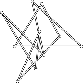
(a) $8_{10}$

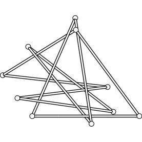
(b) $9_{7}$

Figure 1: Polygonal realizations of the $8_{10}$ and $9_{7}$ knots. These curves both have superbridge number equal to 4: each has 4 local maxima when projected to the $x$-axis, so the superbridge number is at least 4, and Corollary 9 will imply that superbridge number is $\leq 4$. Each knot is shown in orthographic perspective, viewed from the direction of the positive $z$-axis relative to the vertex coordinates given in Appendix C.

The main contribution of the present paper is a new approach to giving upper bounds on superbridge index. In some sense the approach is obvious: find a realization of a knot $K$ whose superbridge number is no bigger than some $m$, and conclude that $\operatorname{sb}[K]\leq m$. The challenge comes in showing that, for a given realization of $K$, there is no direction so that projecting to a line in that direction has more than $m$ local maxima. The strategy in this paper is to use polygonal realizations and to observe that the existence of a direction with $m+1$ local maxima is equivalent to the feasibility of a system of linear inequalities. In other words, ruling out the existence of such directions is equivalent to showing that the system has no solutions, which will be done using Gordan’s Theorem [18], a classical linear programming tool for certifying the non-existence of solutions.

See Figure 1 for two such polygonal realizations of the knots $8_{10}$ and $9_{7}$. Both will be shown to have superbridge number $\leq 4$, and hence it will follow that $\operatorname{sb}[8_{10}],\operatorname{sb}[9_{7}]\leq 4$. More generally, the main theorem of this paper is:

Theorem 1.

The knots $8_{1-15}$, $9_{7}$, $9_{16}$, $9_{20}$, $9_{26}$, $9_{28}$, $9_{32}$, and $9_{33}$ have superbridge index $\leq 4$, and $10_{76}$, $13n_{226}$, $13n_{328}$, $13n_{342}$, $13n_{343}$, $13n_{350}$, $13n_{512}$, $13n_{973}$, $13n_{2641}$, $13n_{5018}$, and $14n_{1753}$ have superbridge index $\leq 5$.

This implies that the knots $8_{1}$, $8_{2}$, $8_{3}$, $8_{5}$, $8_{6}$, $8_{7}$, $8_{8}$, $8_{10}$, $8_{11}$, $8_{12}$, $8_{13}$, $8_{14}$, $8_{15}$, $9_{7}$, $9_{16}$, $9_{20}$, $9_{26}$, $9_{28}$, $9_{32}$, and $9_{33}$ have superbridge index equal to 4, and that $13n_{226}$, $13n_{328}$, $13n_{342}$, $13n_{343}$, $13n_{350}$, $13n_{512}$, $13n_{973}$, $13n_{2641}$, $13n_{5018}$, and $14n_{1753}$ have superbridge index equal to 5.

The particular polygonal realizations providing these bounds were found by generating large ensembles of random equilateral polygons in tight confinement using the algorithm described in the paper [15] and implemented in the open-source stick-knot-gen project [14].

Section 2 below gives some background on superbridge index, including a survey of known bounds. The connection to Gordan’s theorem is explained in Section 3, which is where Theorem 1 is proved, and Section 4 provides some discussion and open questions. Appendix A consists of a table of values (or possible values, when the exact value is not known) of the superbridge index for all prime knots through 10 crossings, Appendix B gives all prime knots through 16 crossings for which the exact value of superbridge index is known, Appendix C gives the coordinates for each of the polygonal knots discussed in this paper (which can also be downloaded from the stick-knot-gen project [14]), and Appendix D gives diagrams for the 13- and 14-crossing knots and homomorphisms from each knot group to the symmetric group $S_{5}$ which will be used in the proof of Theorem 1.

2 Background on the Superbridge Index

The only infinite class of prime knots for which superbridge index is known is the class of torus knots:

Theorem 2 (Kuiper [23]).

For relatively prime $2\leq p<q$, the superbridge index of the $(p,q)$-torus knot is

$$\operatorname{sb}[T_{p,q}]=\min(2p,q).$$

Progress in determining the superbridge index of knots has been slow. Aside from torus knots, the superbridge index was known for only 41 prime knots prior to the present work. In particular, it was known for only 29 of the 249 nontrivial knots with 10 or fewer crossings. In virtually all cases, the strategy for computing superbridge index is to show that some upper bound matches a lower bound.

The most useful lower bounds on superbridge index are:

Theorem 3 (Kuiper [23]).

For any nontrivial knot $K$, the bridge index $\operatorname{b}[K]<\operatorname{sb}[K]$.

Theorem 4 (Jeon–Jin [20]).

Every knot except $3_{1}$ and $4_{1}$ and possibly $5_{2}$, $6_{1}$, $6_{2}$, $6_{3}$, $7_{2}$, $7_{3}$, $7_{4}$, $8_{4}$, and $8_{9}$ has superbridge index $\geq 4$.

This is slightly different than the statement in Jeon and Jin’s paper, which included $8_{7}$ in the list of possible 3-superbridge knots. However, $8_{7}$ cannot have superbridge index equal to 3:

Lemma 5.

$\operatorname{sb}[8_{7}]\geq 4$.

Proof.

This result was first proved by Adams et al. in an early version of their paper [2]; their proof, which is essentially the one given below, was also sketched in a talk given by Gyo Taek Jin in February, 2020 [21].

Jeon and Jin’s characterization of possible 3-superbridge knots begins by assuming that a given parametrization $\gamma:S^{1}\to\mathbb{R}^{3}$ of a nontrivial knot has superbridge number 3, projecting to the orthogonal complement of a quadrisecant—a line whose intersection with the image of $\gamma$ consists of at least 4 distinct components—and using the assumption $\operatorname{sb}(\gamma)=3$ to constrain the resulting planar curve, and hence the possible knot types of $\gamma$.

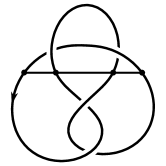
(a) Simple

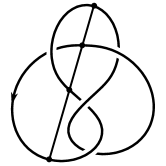
(b) Flipped

(c) Alternating

Figure 2: The three types of quadrisecant illustrated on the figure eight knot from KnotPlot [36]. Traversing the curve in the direction of the indicated orientation starting at point $a$ produces the word $acbd$ for the alternating quadrisecant, as opposed to $abcd$ for the simple quadrisecant and $abdc$ for the flipped quadrisecant.

The fact that $\gamma$ has a quadrisecant was proved by Kuperberg [24], building on work of Pannwitz [32] and Morton and Mond [28], but Denne has proved [12, 13] that every nontrivial knot has an alternating quadrisecant; see Figure 2. Therefore, Jeon and Jin’s argument can be modified to require the quadrisecant of $\gamma$ be alternating. However, all the $8_{7}$ knots in their catalog (one in their Table T and two in Table V) are associated with a non-alternating quadrisecant, contradicting this assumption and proving that $8_{7}$ cannot have superbridge index equal to 3. ∎

By far the most useful upper bound on superbridge index is given in terms of stick number.

Theorem 6 (Jin [22]).

For any knot $K$, $\operatorname{sb}[K]\leq\frac{1}{2}\operatorname{stick}[K]$.

This follows because the projection of a polygonal knot to a line cannot have more critical points than vertices. To date, all determinations of superbridge indices of non-torus knots have come from matching this upper bound with one of the lower bounds from Theorems 3 or 4. In particular, this accounts for all exact values of superbridge index in Appendix B aside from those for torus knots and those attributable to Theorem 1.

As mentioned in the introduction, this strategy cannot work in general: for any $n$ there are only finitely many knots with $\operatorname{stick}[K]\leq n$ [9, 31], but there are infinitely many 2-bridge knots and hence, by the next theorem, infinitely many knots with $\operatorname{sb}[K]\leq 5$.

Theorem 7 (Adams et al. [2]).

For any knot $K$, $\operatorname{sb}[K]\leq 3\operatorname{b}[K]-1$.

This bound is somewhat weaker than the one announced in [1], but it is still a significant improvement on the bound $\operatorname{sb}[K]\leq 5\operatorname{b}[K]-3$ proved by Furstenberg, Li, and Schneider [17]. Notice, in particular, that this theorem implies $\operatorname{sb}[10_{37}]\leq 5$, even though the best extant bound on stick number is $\operatorname{stick}[10_{37}]\leq 12$ [15].

Superbridge index is also bounded above by twice the braid index [23] and by the harmonic index [37, 38], though these are less useful: the only knots through 11 crossings for which either of these bounds is better than those from Theorems 6 and 7 are the 3-braid knots $11a_{240}$ and $11a_{338}$, both of which have bridge index 3 [30] and no known bound on stick number besides the general bound $\operatorname{stick}[K]\leq 18$ for all 11-crossing knots [19].

3 A New Approach

One of the major challenges in computing superbridge index is that the inequalities go the wrong way: if $\gamma$ is a closed curve in $\mathbb{R}^{3}$ and the projection of $\gamma$ to a line has $m$ local maxima, this shows that $\operatorname{sb}(\gamma)\geq m$. But this gives no information about $\operatorname{sb}[\gamma]$, since there could well be some other line on which the projection of $\gamma$ has $m+1$ local maxima (contrast with bridge index: in the hypothetical, it follows that $\operatorname{b}[\gamma]\leq\operatorname{b}(\gamma)\leq m$). This means it is not so easy to use particular realizations of a knot to give bounds on superbridge index.

Working with polygonal knots—that is, piecewise linear embeddings $\gamma:S^{1}\to\mathbb{R}^{3}$—discretizes the problem and will turn out to yield bounds coming from Gordan’s theorem. Rather than thinking in terms of the parametrization, it will be more convenient to represent polygonal knots by a list $\vec{e}_{1},\dots,\vec{e}_{n}$ of edge vectors.

In those terms,

$$\operatorname{b}_{\vec{v}}(\vec{e}_{1},\dots,\vec{e}_{n})=\#\{i\in[n]:\vec{e}_{i}\cdot\vec{v}>0\text{ and }\vec{e}_{i+1}\cdot\vec{v}<0\}$$

with the convention that $\vec{e}_{n+1}=\vec{e}_{1}$. Here $\cdot$ is the usual dot product on $\mathbb{R}^{3}$.

The proof of Theorem 6 implies that $\operatorname{sb}(\vec{e}_{1},\dots,\vec{e}_{n})\leq\frac{n}{2}$. Equality is achieved in this bound if and only if $n$ is even and the projection of each vertex to the line spanned by some $\vec{v}\in S^{2}$ is either a local minimum or a local maximum. In particular, this means that the list

$$\vec{v}\cdot\vec{e}_{1},\vec{v}\cdot\vec{e}_{2},\dots,\vec{v}\cdot\vec{e}_{n}$$

must alternate signs. By replacing $\vec{v}$ with $-\vec{v}$ if necessary, it is no restriction to assume that $\vec{v}\cdot\vec{e}_{1}>0$, so that the sign pattern is $+1,-1,\dots,-1$.

Equivalently, if $n$ is even and

$$E=\left[\vec{e}_{1}|-\vec{e}_{2}|\cdots|-\vec{e}_{n}\right]$$

is the $3\times n$ matrix with the $(-1)^{i+1}\vec{e}_{i}$ as its columns, $\operatorname{sb}(\vec{e}_{1},\dots,\vec{e}_{n})<\frac{n}{2}$ if and only if there is no $\vec{v}\in\mathbb{R}^{3}$ so that $\vec{v}^{T}E$ has all positive entries. Contrapositively, the linear system $\vec{v}^{T}E>0$ has a solution if and only if $\operatorname{sb}(\vec{e}_{1},\dots,\vec{e}_{n})=\frac{n}{2}$.

Gordan’s theorem is a key tool for determining whether such systems of linear inequalities have solutions:

Theorem 8 (Gordan [18]).

Suppose $A$ is a $k\times\ell$ real matrix. Then exactly one of the following is true:

1. There exists $\vec{v}\in\mathbb{R}^{k}$ so that $\vec{v}^{T}A$ has all positive entries.

2. $A\vec{u}=\vec{0}$ for some nonzero vector $\vec{u}\in\mathbb{R}^{\ell}$ with nonnegative entries.

Among the class of theorems called theorems of the alternative (see, e.g., [39] or [11, §2.4]), Gordan’s theorem was the first to appear, predating Farkas’ Lemma [16] by almost 30 years. Here is an intuitive explanation of why Gordan’s theorem is true: if (i) is true, then the angles between $\vec{v}$ and each of the columns of $A$ are all less than $90^{\circ}$. But in this case the columns of $A$ all lie in the interior of a half-space, and no (nontrivial) conical combination produces the origin. On the other hand, (ii) says exactly that the origin is a conical combination of the columns of $A$.

Gordan’s theorem, combined with the preceding discussion, yields the following immediate corollary:

Corollary 9.

If $n$ is even and $\vec{e}_{1},\dots,\vec{e}_{n}$ are the edge vectors of a closed polygonal curve in $\mathbb{R}^{3}$, then $\operatorname{sb}(\vec{e}_{1},\dots,\vec{e}_{n})<\frac{n}{2}$ if and only if there exists a nonzero vector $\vec{u}\in\mathbb{R}^{n}$ with nonnegative entries solving the matrix equation

$$\left[\vec{e}_{1}|-\vec{e}_{2}|\cdots|-\vec{e}_{n}\right]\vec{u}=\vec{0}.$$ (1)

The vector $\vec{u}$ solving (1) provides a certificate that there is no line onto which the polygonal curve can be projected with $\frac{n}{2}$ local maxima. This corollary is the essential result needed to prove Theorem 1.

Theorem 1.

The knots $8_{1-15}$, $9_{7}$, $9_{16}$, $9_{20}$, $9_{26}$, $9_{28}$, $9_{32}$, and $9_{33}$ have superbridge index $\leq 4$, and $10_{76}$, $13n_{226}$, $13n_{328}$, $13n_{342}$, $13n_{343}$, $13n_{350}$, $13n_{512}$, $13n_{973}$, $13n_{2641}$, $13n_{5018}$, and $14n_{1753}$ have superbridge index $\leq 5$.

This implies that the knots $8_{1}$, $8_{2}$, $8_{3}$, $8_{5}$, $8_{6}$, $8_{7}$, $8_{8}$, $8_{10}$, $8_{11}$, $8_{12}$, $8_{13}$, $8_{14}$, $8_{15}$, $9_{7}$, $9_{16}$, $9_{20}$, $9_{26}$, $9_{28}$, $9_{32}$, and $9_{33}$ have superbridge index equal to 4, and that $13n_{226}$, $13n_{328}$, $13n_{342}$, $13n_{343}$, $13n_{350}$, $13n_{512}$, $13n_{973}$, $13n_{2641}$, $13n_{5018}$, and $14n_{1753}$ have superbridge index equal to 5.

Proof.

Coordinates of the vertices of polygonal realizations of each of these knots are given in Appendix C along with visualizations. For example, the entry for the $8_{5}$ knot is repeated in Table 1. The polygons were originally generated with coordinates given as double-precision floating point numbers, but to make it easier to verify the existence of exact solutions to (1) these coordinates were rounded to three significant digits and converted to integers (while verifying that this did not change the knot type).

	$0$	$0$	$0$	$1$
	$1000$	$0$	$0$	$1$
	$155$	$535$	$0$	$8061667015$
	$57$	$-456$	$94$	$1$
	$572$	$183$	$-478$	$1$
	$842$	$108$	$482$	$1$
	$-104$	$233$	$181$	$496072961$
	$781$	$398$	$-254$	$2237736971$
	$482$	$-67$	$579$	$3514960071$
	$182$	$877$	$444$	$4046282755$

Table 1: Visualization of a 10-stick realization of the $8_{5}$ knot and the coordinates of its vertices. The rightmost column gives the entries of the vector $\vec{u}$ solving the equation in Corollary 9.

In each case, the superbridge index bound will follow from Corollary 9, so the goal is to find an appropriate $\vec{u}$. In the case of $8_{5}$, it suffices to find a nonzero vector $\vec{u}$ with nonnegative entries so that

$$\begin{bmatrix}1000&845&-98&-515&270&946&885&299&-300&182\\ 0&-535&-991&-639&-75&-125&165&465&944&877\\ 0&0&94&572&960&301&-435&-833&-135&444\end{bmatrix}\vec{u}=\begin{bmatrix}0\\ 0\\ 0\end{bmatrix}.$$ (2)

The columns in the $3\times 10$ matrix above are $(-1)^{i+1}\vec{e}_{i}$, where the $i$th edge vector $\vec{e}_{i}=\vec{v}_{i+1}-\vec{v}_{i}$, the vertices $\vec{v}_{j}$ have coordinates given in Table 1, and indices are computed cyclically so that $\vec{e}_{10}=\vec{v}_{1}-\vec{v}_{10}$.

It is straightforward to verify that

$$\vec{u}=(1,\,1,\,8061667015,\,1,\,1,\,1,\,496072961,\,2237736971,\,3514960071,\,4046282755)$$

is a vector with all positive entries solving (2), so this vector in conjunction with Corollary 9 certifies that the superbridge number of this realization of $8_{5}$ is less than 5, and hence that $\operatorname{sb}[8_{5}]\leq 4$. The entries in $\vec{u}$ are given in the rightmost column in Table 1.

A similar argument works for each of the knots in the statement of the theorem: particular vectors $\vec{u}$ solving the equation in Corollary 9 are given in the rightmost column of each table in Appendix C. The certificate vectors $\vec{u}$ were found using Mathematica’s FindInstance function.

The second sentence in the statement of the theorem follows from observing that the upper bounds just proved match lower bounds coming from Theorems 3 and 4. Specifically, the knots $8_{1}$, $8_{2}$, $8_{3}$, $8_{5}$, $8_{6}$, $8_{7}$, $8_{8}$, $8_{10}$, $8_{11}$, $8_{12}$, $8_{13}$, $8_{14}$, $8_{15}$, $9_{7}$, $9_{16}$, $9_{20}$, $9_{26}$, $9_{32}$, and $9_{33}$ all have superbridge index $\geq 4$ by Theorem 4, and hence their superbridge index must be exactly 4.

As for the higher-crossing knots, the result will follow if their bridge indices are bounded below by 4, since then Theorem 3 implies that their superbridge indices are at least 5. Using Lemma 10—stated below—in each case it suffices to find a surjective homomorphism $\pi_{1}(S^{3}\backslash K)\!\twoheadrightarrow S_{5}$ from the knot group $\pi_{1}(S^{3}\backslash K)$ to the symmetric group $S_{5}$ sending meridians to transpositions. Table 2 shows a diagram of $13n_{350}$ with strand labels defining such a homomorphism. Specifically, labeling the strand $(-7,-5)$ with the transposition $(1\,2)$, the strand $(-8,9,-10)$ with $(1\,3)$, the strand $(-6,7,11,-9)$ with $(1\,4)$, and the strand $(-2,3,-1)$ with $(2\,5)$ induces a complete labeling of strands when the labels are propagated to the other strands via the Wirtinger relations. This labeling satisfies the Wirtinger relations by construction and $\{(1\,2),(1\,3),(1\,4),(2\,5)\}$ is a generating set for $S_{5}$, so this induces the desired surjective homomorphism $\pi_{1}(S^{3}\backslash 13n_{350})\!\twoheadrightarrow S_{5}$.

Appendix D gives similar homomorphisms for each of 13- and 14-crossing knots in the statement of the theorem, completing the proof. All of these homomorphisms were found using a preliminary version of Wirt_Hm_Suite [27], which is being developed as part of forthcoming work by Blair, Kjuchukova, and Morrison [7]. ∎

The following lemma giving a lower bound in bridge index is well-known. It is a classical example of a more general strategy that gives lower bounds on bridge index by finding a surjective homomorphism from the knot group to a group with nice properties [4, 5].

Lemma 10.

Let $K$ be a knot and $S_{n}$ the symmetric group on $n$ elements. If the knot group $\pi_{1}\!\left(S^{3}\,\backslash K\right)\!$ admits a surjective homomorphism to $S_{n}$ such that every meridian is sent to a transposition, then $\operatorname{b}[K]\geq n-1$.

$13n_{350}$
	$(-7,-5)$	$\mapsto(1\,2)$
	$(-8,9,-10)$	$\mapsto(1\,3)$
	$(-6,7,11,-9)$	$\mapsto(1\,4)$
	$(-2,3,-1)$	$\mapsto(2\,5)$

Table 2: The SnapPy [10] diagram of $13n_{350}$ with crossings labeled $1,2,\dots,13$. A surjective homomorphism $\pi_{1}(S^{3}\backslash 13n_{350})\twoheadrightarrow S_{5}$ is defined by mapping Wirtinger generators to transpositions as indicated to the right. The strands in the diagram, which correspond to Wirtinger generators, are specified by indicating the under crossings at which each strand begins and ends, and the over crossings (if any) along the way. For example, $(-6,7,11,-9)$ starts at the under strand of crossing 6, passes over crossings 7 and 11, and then ends as the under strand at crossing 9. The images of the remaining Wirtinger generators are determined by applying the Wirtinger relations at each crossing. In this diagram (though not in the diagrams in Appendix D), all strands are labelled with their image in $S_{5}$; the generating labels are bolded.

4 Conclusion

The superbridge index remains frustratingly unknown for all the knots mentioned in Theorem 4 except $3_{1}$ and $4_{1}$. Theorem 1 eliminated the possibility that $\operatorname{sb}[8_{4}]$ or $\operatorname{sb}[8_{9}]$ is equal to 5, so each of the knots $5_{2}$, $6_{1}$, $6_{2}$, $6_{3}$, $7_{2}$, $7_{3}$, $7_{4}$, $8_{4}$, and $8_{9}$ has superbridge index equal to either 3 or 4.

Conjecture 11 (Jeon–Jin [20]).

The only knots with superbridge index equal to 3 are $3_{1}$ and $4_{1}$.

While the approach using Gordan’s theorem described in Section 3 above cannot help prove this conjecture, it might be useful in finding a counterexample if one exists.

The specific polygonal realizations of knots used in the proof of Theorem 1 were found by generating large ensembles of random equilateral polygons in tight confinement using the algorithm described in [15]. Between Theorem 1 and previous work [6, 15], upper bounds coming from random polygons generated in this way have increased the total number of prime, non-torus knots for which superbridge index is known from 23 to 71. While there are limits to this approach, especially in the absence of more refined lower bounds on superbridge index, its usefulness is probably not yet entirely exhausted. In the future, it might be helpful to explore algorithms for generating polygons with variable (rather than fixed) edgelengths in tight confinement.

Finally, there is a paucity of useful lower bounds on superbridge index beyond those given in Theorems 3 and 4 (Adams et al. [3] notwithstanding). Lower bounds coming from algebraic information—analogous to the bridge index bound from Lemma 10—would be particularly welcome and might dramatically expand our ability to compute superbridge indices of particular knots.

Acknowledgments

I am grateful to Jason Cantarella for introducing me to random polygons, to Tom Eddy for getting me serious about generating massive ensembles of them, and to Ryan Blair for sharing his knowledge about bridge index. As usual, thanks to Allison Moore and Chuck Livingston for maintaining KnotInfo [25], which is an invaluable resource. This work was partially supported by grants from the Simons Foundation (#354225 and #709150).

Appendix A Table of Superbridge Indices

Superbridge indices for prime knots through 10 crossings are given below, including references for where these results were proved. If the exact superbridge index is not known, the possible values, as determined by known upper and lower bounds, are given.

In all cases, the lower bound comes from either Kuiper’s result $\operatorname{b}[K]<\operatorname{sb}[K]$ [23, stated as Theorem 3 above] or Jeon and Jin’s characterization of 3-superbridge knots [20, stated as Theorem 4 above], so these references are not explicitly included in the table below. Most of the upper bounds come from Jin’s bound $\operatorname{sb}[K]\leq\frac{1}{2}\operatorname{stick}[K]$ [22, stated as Theorem 6 above], but not all (e.g., $8_{4}$, $10_{37}$, and $10_{76}$), so this reference is included when relevant, along with reference(s) to the best upper bound on stick number. An up-to-date table of stick number bounds is given in [15] or online at the stick-knot-gen project [14].

$K$	$\operatorname{sb}[K]$
$0_{1}$	1
$3_{1}$	3	[23]
$4_{1}$	3	[22, 33]
$5_{1}$	4	[23]
$5_{2}$	3 or 4	[22]
$6_{1}$	3 or 4	[22, 31, 26]
$6_{2}$	3 or 4	[22, 31, 26]
$6_{3}$	3 or 4	[22, 31, 26]
$7_{1}$	4	[23]
$7_{2}$	3 or 4	[22, 26]
$7_{3}$	3 or 4	[22, 26]
$7_{4}$	3 or 4	[22, 26]
$7_{5}$	4	[22, 26]
$7_{6}$	4	[22, 26]
$7_{7}$	4	[22, 26]
$8_{1}$	4	Theorem 1
$8_{2}$	4	Theorem 1
$8_{3}$	4	Theorem 1
$8_{4}$	3 or 4	Theorem 1
$8_{5}$	4	Theorem 1
$8_{6}$	4	Theorem 1
$8_{7}$	4	Theorem 1
$8_{8}$	4	Theorem 1
$8_{9}$	3 or 4	Theorem 1
$8_{10}$	4	Theorem 1
$8_{11}$	4	Theorem 1
$8_{12}$	4	Theorem 1
$8_{13}$	4	Theorem 1
$8_{14}$	4	Theorem 1
$8_{15}$	4	Theorem 1
$8_{16}$	4	[22, 34]
$8_{17}$	4	[22, 34]
$8_{18}$	4	[9, 22, 34]
$8_{19}$	4	[23]
$8_{20}$	4	[22, 31, 26]
$8_{21}$	4	[22, 26]
$9_{1}$	4	[23]
$9_{2}$	4 or 5	[15, 22]
$9_{3}$	4 or 5	[15, 22]
$9_{4}$	4 or 5	[22, 34]
$9_{5}$	4 or 5	[22, 34]
$9_{6}$	4 or 5	[22, 34]
$9_{7}$	4	Theorem 1
$9_{8}$	4 or 5	[22, 34]
$9_{9}$	4 or 5	[22, 34]
$9_{10}$	4 or 5	[22, 34]
$9_{11}$	4 or 5	[15, 22]
$9_{12}$	4 or 5	[22, 34]
$9_{13}$	4 or 5	[22, 34]
$9_{14}$	4 or 5	[22, 34]
$9_{15}$	4 or 5	[15, 22]
$9_{16}$	4	Theorem 1
$9_{17}$	4 or 5	[22, 34]
$9_{18}$	4 or 5	[22, 34]
$9_{19}$	4 or 5	[22, 34]
$9_{20}$	4	Theorem 1
$9_{21}$	4 or 5	[15, 22]
$9_{22}$	4 or 5	[22, 34]
$9_{23}$	4 or 5	[22, 34]
$9_{24}$	4 or 5	[22, 34]
$9_{25}$	4 or 5	[15, 22]
$9_{26}$	4	Theorem 1
$9_{27}$	4 or 5	[15, 22]
$9_{28}$	4	Theorem 1
$9_{29}$	4	[22, 35]
$9_{30}$	4 or 5	[22, 34]
$9_{31}$	4 or 5	[22, 34]
$9_{32}$	4	Theorem 1
$9_{33}$	4	Theorem 1
$9_{34}$	4	[22, 34]
$9_{35}$	4	[15, 22]
$9_{36}$	4 or 5	[22, 34]
$9_{37}$	4 or 5	[22, 34]
$9_{38}$	4 or 5	[22, 34]
$9_{39}$	4	[15, 22]
$9_{40}$	4	[22]
$9_{41}$	4	[22]
$9_{42}$	4	[22]
$9_{43}$	4	[15, 22]
$9_{44}$	4	[22, 34]
$9_{45}$	4	[15, 22]
$9_{46}$	4	[22]
$9_{47}$	4	[22, 34]
$9_{48}$	4	[15, 22]
$9_{49}$	4	[22, 34]
$10_{1}$	4 or 5	[22, 34]
$10_{2}$	4 or 5	[22, 34]
$10_{3}$	4 or 5	[15, 22]
$10_{4}$	4 or 5	[22, 34]
$10_{5}$	4 or 5	[22, 34]
$10_{6}$	4 or 5	[15, 22]
$10_{7}$	4 or 5	[15, 22]
$10_{8}$	4 or 5	[15, 22]
$10_{9}$	4 or 5	[22, 34]
$10_{10}$	4 or 5	[15, 22]
$10_{11}$	4 or 5	[22, 34]
$10_{12}$	4 or 5	[22, 34]
$10_{13}$	4 or 5	[22, 34]
$10_{14}$	4 or 5	[22, 34]
$10_{15}$	4 or 5	[15, 22]
$10_{16}$	4 or 5	[15, 22]
$10_{17}$	4 or 5	[15, 22]
$10_{18}$	4 or 5	[15, 22]
$10_{19}$	4 or 5	[22, 34]
$10_{20}$	4 or 5	[15, 22]
$10_{21}$	4 or 5	[15, 22]
$10_{22}$	4 or 5	[15, 22]
$10_{23}$	4 or 5	[15, 22]
$10_{24}$	4 or 5	[15, 22]
$10_{25}$	4 or 5	[22, 34]
$10_{26}$	4 or 5	[15, 22]
$10_{27}$	4 or 5	[22, 34]
$10_{28}$	4 or 5	[15, 22]
$10_{29}$	4 or 5	[22, 34]
$10_{30}$	4 or 5	[15, 22]
$10_{31}$	4 or 5	[15, 22]
$10_{32}$	4 or 5	[22, 34]
$10_{33}$	4 or 5	[22, 34]
$10_{34}$	4 or 5	[15, 22]
$10_{35}$	4 or 5	[15, 22]
$10_{36}$	4 or 5	[22, 34]
$10_{37}$	4 or 5	[2]
$10_{38}$	4 or 5	[15, 22]
$10_{39}$	4 or 5	[15, 22]
$10_{40}$	4 or 5	[22, 34]
$10_{41}$	4 or 5	[22, 34]
$10_{42}$	4 or 5	[22, 34]
$10_{43}$	4 or 5	[15, 22]
$10_{44}$	4 or 5	[15, 22]
$10_{45}$	4 or 5	[22, 34]
$10_{46}$	4 or 5	[15, 22]
$10_{47}$	4 or 5	[15, 22]
$10_{48}$	4 or 5	[22, 34]
$10_{49}$	4 or 5	[22, 34]
$10_{50}$	4 or 5	[15, 22]
$10_{51}$	4 or 5	[15, 22]
$10_{52}$	4 or 5	[22, 34]
$10_{53}$	4 or 5	[15, 22]
$10_{54}$	4 or 5	[15, 22]
$10_{55}$	4 or 5	[15, 22]
$10_{56}$	4 or 5	[15, 22]
$10_{57}$	4 or 5	[15, 22]
$10_{58}$	4, 5, or 6	[22, 34]
$10_{59}$	4 or 5	[22, 34]
$10_{60}$	4 or 5	[22, 34]
$10_{61}$	4 or 5	[22, 34]
$10_{62}$	4 or 5	[15, 22]
$10_{63}$	4 or 5	[22, 34]
$10_{64}$	4 or 5	[15, 22]
$10_{65}$	4 or 5	[15, 22]
$10_{66}$	4, 5, or 6	[22, 34]
$10_{67}$	4 or 5	[22, 34]
$10_{68}$	4 or 5	[15, 22]
$10_{69}$	4 or 5	[22, 34]
$10_{70}$	4 or 5	[15, 22]
$10_{71}$	4 or 5	[15, 22]
$10_{72}$	4 or 5	[15, 22]
$10_{73}$	4 or 5	[15, 22]
$10_{74}$	4 or 5	[15, 22]
$10_{75}$	4 or 5	[15, 22]
$10_{76}$	4 or 5	Theorem 1
$10_{77}$	4 or 5	[15, 22]
$10_{78}$	4 or 5	[15, 22]
$10_{79}$	4 or 5	[22, 35]
$10_{80}$	4, 5, or 6	[15, 22]
$10_{81}$	4 or 5	[22, 34]
$10_{82}$	4 or 5	[15, 22]
$10_{83}$	4 or 5	[15, 22]
$10_{84}$	4 or 5	[15, 22]
$10_{85}$	4 or 5	[15, 22]
$10_{86}$	4 or 5	[22, 34]
$10_{87}$	4 or 5	[22, 34]
$10_{88}$	4 or 5	[22, 34]
$10_{89}$	4 or 5	[22, 34]
$10_{90}$	4 or 5	[15, 22]
$10_{91}$	4 or 5	[15, 22]
$10_{92}$	4 or 5	[22, 34]
$10_{93}$	4 or 5	[22, 34]
$10_{94}$	4 or 5	[15, 22]
$10_{95}$	4 or 5	[15, 22]
$10_{96}$	4 or 5	[22, 34]
$10_{97}$	4 or 5	[15, 22]
$10_{98}$	4 or 5	[22, 34]
$10_{99}$	4 or 5	[22, 34]
$10_{100}$	4 or 5	[15, 22]
$10_{101}$	4 or 5	[15, 22]
$10_{102}$	4 or 5	[22, 34]
$10_{103}$	4 or 5	[15, 22]
$10_{104}$	4 or 5	[22, 34]
$10_{105}$	4 or 5	[15, 22]
$10_{106}$	4 or 5	[15, 22]
$10_{107}$	4 or 5	[15, 22, 35]
$10_{108}$	4 or 5	[22, 34]
$10_{109}$	4 or 5	[22, 34]
$10_{110}$	4 or 5	[15, 22]
$10_{111}$	4 or 5	[15, 22]
$10_{112}$	4 or 5	[15, 22]
$10_{113}$	4 or 5	[22, 34]
$10_{114}$	4 or 5	[22, 34]
$10_{115}$	4 or 5	[15, 22]
$10_{116}$	4 or 5	[22, 34]
$10_{117}$	4 or 5	[15, 22]
$10_{118}$	4 or 5	[15, 22]
$10_{119}$	4 or 5	[15, 22, 35]
$10_{120}$	4 or 5	[22, 34]
$10_{121}$	4 or 5	[22, 34]
$10_{122}$	4 or 5	[22, 34]
$10_{123}$	4 or 5	[22, 34]
$10_{124}$	5	[23]
$10_{125}$	4 or 5	[22, 34]
$10_{126}$	4 or 5	[15, 22]
$10_{127}$	4 or 5	[22, 34]
$10_{128}$	4 or 5	[22, 34]
$10_{129}$	4 or 5	[22, 34]
$10_{130}$	4 or 5	[22, 34]
$10_{131}$	4 or 5	[15, 22]
$10_{132}$	4 or 5	[22, 34]
$10_{133}$	4 or 5	[15, 22]
$10_{134}$	4 or 5	[22, 34]
$10_{135}$	4 or 5	[22, 34]
$10_{136}$	4 or 5	[22, 34]
$10_{137}$	4 or 5	[15, 22]
$10_{138}$	4 or 5	[15, 22]
$10_{139}$	4 or 5	[22, 34]
$10_{140}$	4 or 5	[22, 34]
$10_{141}$	4 or 5	[22, 34]
$10_{142}$	4 or 5	[15, 22]
$10_{143}$	4 or 5	[15, 22]
$10_{144}$	4 or 5	[22, 34]
$10_{145}$	4 or 5	[22, 34]
$10_{146}$	4 or 5	[22, 34]
$10_{147}$	4 or 5	[15, 22, 35]
$10_{148}$	4 or 5	[15, 22]
$10_{149}$	4 or 5	[15, 22]
$10_{150}$	4 or 5	[22, 34]
$10_{151}$	4 or 5	[22, 34]
$10_{152}$	4 or 5	[22, 34]
$10_{153}$	4 or 5	[15, 22]
$10_{154}$	4 or 5	[22, 34]
$10_{155}$	4 or 5	[22, 34]
$10_{156}$	4 or 5	[22, 34]
$10_{157}$	4 or 5	[22, 34]
$10_{158}$	4 or 5	[22, 34]
$10_{159}$	4 or 5	[22, 34]
$10_{160}$	4 or 5	[22, 34]
$10_{161}$	4 or 5	[22, 34]
$10_{162}$	4 or 5	[22, 34]
$10_{163}$	4 or 5	[22, 34]
$10_{164}$	4 or 5	[15, 22]
$10_{165}$	4 or 5	[22, 34]

Appendix B Exact Values of Superbridge Index

The prime knots through 16 crossings for which the exact value of superbridge index is known.

$K$	$\operatorname{sb}[K]$
$0_{1}$	1
$3_{1}$	3	[23]
$4_{1}$	3	[22, 33]
$5_{1}$	4	[23]
$7_{1}$	4	[23]
$7_{5}$	4	[22, 26]
$7_{6}$	4	[22, 26]
$7_{7}$	4	[22, 26]
$8_{1}$	4	Theorem 1
$8_{2}$	4	Theorem 1
$8_{3}$	4	Theorem 1
$8_{5}$	4	Theorem 1
$8_{6}$	4	Theorem 1
$8_{7}$	4	Theorem 1
$8_{8}$	4	Theorem 1
$8_{10}$	4	Theorem 1
$8_{11}$	4	Theorem 1
$8_{12}$	4	Theorem 1
$8_{13}$	4	Theorem 1
$8_{14}$	4	Theorem 1
$8_{15}$	4	Theorem 1
$8_{16}$	4	[22, 34]
$8_{17}$	4	[22, 34]
$8_{18}$	4	[9, 22, 34]
$8_{19}$	4	[23]
$8_{20}$	4	[22, 31, 26]
$8_{21}$	4	[22, 26]
$9_{1}$	4	[23]
$9_{7}$	4	Theorem 1
$9_{16}$	4	Theorem 1
$9_{20}$	4	Theorem 1
$9_{26}$	4	Theorem 1
$9_{28}$	4	Theorem 1
$9_{29}$	4	[22, 35]
$9_{32}$	4	Theorem 1
$9_{33}$	4	Theorem 1
$9_{34}$	4	[22, 34]
$9_{35}$	4	[15, 22]
$9_{39}$	4	[15, 22]
$9_{40}$	4	[22]
$9_{41}$	4	[22]
$9_{42}$	4	[22]
$9_{43}$	4	[15, 22]
$9_{44}$	4	[22, 34]
$9_{45}$	4	[15, 22]
$9_{46}$	4	[22]
$9_{47}$	4	[22, 34]
$9_{48}$	4	[15, 22]
$9_{49}$	4	[22, 34]
$10_{124}$	5	[23]
$11a_{367}$	4	[23]
$11n_{71}$	5	[15, 22]
$11n_{73}$	5	[15, 22]
$11n_{74}$	5	[15, 22]
$11n_{75}$	5	[15, 22]
$11n_{76}$	5	[15, 22]
$11n_{78}$	5	[15, 22]
$11n_{81}$	5	[15, 22]
$13a_{4878}$	4	[23]
$13n_{226}$	5	Theorem 1
$13n_{285}$	5	[6, 22]
$13n_{293}$	5	[6, 22]
$13n_{328}$	5	Theorem 1
$13n_{342}$	5	Theorem 1
$13n_{343}$	5	Theorem 1
$13n_{350}$	5	Theorem 1
$13n_{512}$	5	Theorem 1
$13n_{587}$	5	[6, 22]
$13n_{592}$	5	[6, 22]
$13n_{607}$	5	[6, 22]
$13n_{611}$	5	[6, 22]
$13n_{835}$	5	[6, 22]
$13n_{973}$	5	Theorem 1
$13n_{1177}$	5	[6, 22]
$13n_{1192}$	5	[6, 22]
$13n_{2641}$	5	Theorem 1
$13n_{5018}$	5	Theorem 1
$14n_{1753}$	5	Theorem 1
$14n_{21881}$	6	[23]
$15a_{85263}$	4	[23]
$15n_{41126}$	5	[6, 22]
$15n_{41127}$	5	[6, 22]
$15n_{41185}$	5	[23]
$16n_{783154}$	6	[23]

Appendix C Knot Images and Coordinates

Images of and vertex coordinates for each of the knots mentioned in Theorem 1. Each knot is shown in orthographic perspective from the direction of the positive $z$-axis. The first three columns to the right of the image are the coordinates of the vertices, which have been normalized so that the first vertex is at the origin, the second vertex is on the positive $x$-axis, and the third vertex lies in the $xy$-plane with positive $y$-coordinate. The last column gives the entries in the vector $\vec{u}$ satisfying the equation from Corollary 9.

The original floating-point coordinates can be downloaded from the stick-knot-gen project [14].

$8_{1}$
	$0$	$0$	$0$	$1$
	$1000$	$0$	$0$	$1$
	$392$	$794$	$0$	$1$
	$-369$	$229$	$319$	$2864186130$
	$423$	$839$	$330$	$1$
	$220$	$-113$	$101$	$5$
	$306$	$800$	$-299$	$48024948$
	$676$	$367$	$523$	$236163582$
	$-253$	$519$	$185$	$280265709$
	$709$	$705$	$-13$	$2484703250$

$8_{2}$
	$0$	$0$	$0$	$1$
	$1000$	$0$	$0$	$1$
	$401$	$801$	$0$	$27676293106$
	$71$	$170$	$702$	$2$
	$297$	$-357$	$-117$	$1$
	$-71$	$571$	$-174$	$29466942625$
	$194$	$-272$	$294$	$359004357$
	$763$	$473$	$-56$	$19211515592$
	$-90$	$862$	$293$	$494790273$
	$219$	$183$	$958$	$901050440$

$8_{3}$
	$0$	$0$	$0$	$11523814716$
	$1000$	$0$	$0$	$33922449104$
	$437$	$826$	$0$	$1$
	$82$	$89$	$-575$	$1$
	$-355$	$666$	$115$	$1$
	$513$	$601$	$-376$	$1$
	$248$	$-212$	$142$	$9680960$
	$-225$	$436$	$-454$	$41470509758$
	$513$	$-238$	$-456$	$26311260$
	$11$	$534$	$-846$	$79089567$

$8_{4}$
	$0$	$0$	$0$	$82224356775$
	$1000$	$0$	$0$	$1$
	$70$	$366$	$0$	$1$
	$673$	$-413$	$-168$	$1$
	$-49$	$-201$	$491$	$1$
	$186$	$-235$	$-481$	$1$
	$535$	$288$	$297$	$12935105$
	$-159$	$-286$	$-137$	$75530285415$
	$831$	$-349$	$-17$	$12222683491$
	$210$	$-697$	$685$	$713758069$

$8_{5}$
	$0$	$0$	$0$	$1$
	$1000$	$0$	$0$	$1$
	$155$	$535$	$0$	$8061667015$
	$57$	$-456$	$94$	$1$
	$572$	$183$	$-478$	$1$
	$842$	$108$	$482$	$1$
	$-104$	$233$	$181$	$496072961$
	$781$	$398$	$-254$	$2237736971$
	$482$	$-67$	$579$	$3514960071$
	$182$	$877$	$444$	$4046282755$

$8_{6}$
	$0$	$0$	$0$	$1$
	$1000$	$0$	$0$	$1$
	$468$	$847$	$0$	$13996103539$
	$783$	$-100$	$-68$	$1$
	$238$	$-712$	$-640$	$12357524765$
	$-141$	$183$	$-406$	$744803262$
	$519$	$-310$	$161$	$1157872283$
	$702$	$611$	$-183$	$1254460956$
	$395$	$-121$	$425$	$402371992$
	$764$	$-480$	$-432$	$27243476$

$8_{7}$
	$0$	$0$	$0$	$1$
	$1000$	$0$	$0$	$1$
	$26$	$228$	$0$	$993497797$
	$476$	$-198$	$785$	$1$
	$548$	$659$	$276$	$3$
	$-97$	$-18$	$-77$	$1004972499$
	$841$	$171$	$212$	$16597981$
	$356$	$358$	$-642$	$135013158$
	$89$	$68$	$277$	$601139748$
	$632$	$742$	$-224$	$223374715$

$8_{8}$
	$0$	$0$	$0$	$1261677133211$
	$10000$	$0$	$0$	$1$
	$3086$	$7225$	$0$	$130835438045$
	$3093$	$-2773$	$-206$	$1$
	$6857$	$5129$	$4632$	$1$
	$-2809$	$2567$	$4514$	$1$
	$5157$	$6374$	$-183$	$1430647762564$
	$-4789$	$6789$	$767$	$166227086780$
	$3281$	$2871$	$5184$	$3491957024$
	$9811$	$242$	$-1919$	$298663293981$

$8_{9}$
	$0$	$0$	$0$	$1$
	$1000$	$0$	$0$	$1$
	$302$	$716$	$0$	$1$
	$332$	$-284$	$19$	$1$
	$265$	$520$	$-573$	$12525679$
	$50$	$-143$	$144$	$129465454$
	$926$	$55$	$-295$	$7720205$
	$488$	$373$	$546$	$5545652$
	$-18$	$-175$	$-121$	$24812819$
	$815$	$169$	$-554$	$117804943$

$8_{10}$
	$0$	$0$	$0$	$1$
	$1000$	$0$	$0$	$1$
	$262$	$674$	$0$	$1$
	$433$	$-130$	$569$	$1$
	$-197$	$506$	$123$	$1$
	$316$	$-334$	$-54$	$5014949497$
	$374$	$225$	$773$	$250995749$
	$41$	$-525$	$203$	$370150061$
	$670$	$152$	$-179$	$2517248393$
	$405$	$640$	$653$	$3146528061$

$8_{11}$
	$0$	$0$	$0$	$1$
	$1000$	$0$	$0$	$1$
	$113$	$462$	$0$	$1$
	$636$	$-387$	$71$	$1$
	$194$	$203$	$-605$	$29374052043$
	$304$	$-194$	$307$	$9395661114$
	$830$	$447$	$-253$	$53279952$
	$330$	$-176$	$-855$	$793938322$
	$570$	$-354$	$99$	$35840609905$
	$622$	$136$	$-771$	$103610091$

$8_{12}$
	$0$	$0$	$0$	$1$
	$1000$	$0$	$0$	$1$
	$463$	$843$	$0$	$1$
	$749$	$-85$	$237$	$1$
	$-55$	$-97$	$-358$	$14648534110$
	$304$	$580$	$284$	$1$
	$-409$	$518$	$-414$	$272953947$
	$237$	$-206$	$-171$	$10328384040$
	$530$	$717$	$80$	$6335908245$
	$122$	$560$	$-819$	$1443566304$

$8_{13}$
	$0$	$0$	$0$	$1$
	$1000$	$0$	$0$	$1$
	$198$	$597$	$0$	$1$
	$404$	$-380$	$51$	$560401500$
	$490$	$249$	$823$	$1$
	$102$	$-666$	$715$	$7$
	$429$	$-118$	$-55$	$265466226$
	$266$	$847$	$147$	$283945161$
	$869$	$136$	$-214$	$11280336$
	$681$	$-260$	$685$	$388847518$

$8_{14}$
	$0$	$0$	$0$	$1$
	$1000$	$0$	$0$	$1$
	$164$	$549$	$0$	$22986044$
	$505$	$-391$	$-14$	$1$
	$495$	$435$	$-577$	$1$
	$169$	$256$	$351$	$112$
	$292$	$-306$	$-467$	$2101619$
	$-74$	$362$	$181$	$17826677$
	$616$	$-295$	$-123$	$3072051$
	$572$	$609$	$-549$	$9382065$

$8_{15}$
	$0$	$0$	$0$	$1$
	$1000$	$0$	$0$	$1197682194$
	$375$	$781$	$0$	$1$
	$-31$	$220$	$722$	$1$
	$53$	$-46$	$-239$	$2$
	$146$	$626$	$496$	$3$
	$837$	$-97$	$517$	$647898942$
	$21$	$311$	$109$	$373521904$
	$835$	$-174$	$-208$	$345796927$
	$650$	$749$	$129$	$227928351$

$9_{7}$
	$0$	$0$	$0$	$1$
	$1000$	$0$	$0$	$1422508933$
	$407$	$805$	$0$	$1$
	$-275$	$382$	$-597$	$1$
	$703$	$272$	$-420$	$60828916$
	$-138$	$168$	$111$	$60828918$
	$756$	$41$	$-318$	$928107766$
	$-38$	$648$	$-346$	$10477918$
	$553$	$-72$	$20$	$420725157$
	$401$	$915$	$-34$	$172196045$

$9_{16}$
	$0$	$0$	$0$	$1$
	$1000$	$0$	$0$	$1326961294$
	$291$	$706$	$0$	$1$
	$1046$	$460$	$609$	$1$
	$804$	$450$	$-361$	$1338798152$
	$114$	$519$	$359$	$1$
	$1097$	$475$	$180$	$47421860$
	$223$	$261$	$-257$	$618252967$
	$867$	$-122$	$405$	$442800719$
	$771$	$539$	$-339$	$603197992$

$9_{20}$
	$0$	$0$	$0$	$1$
	$1000$	$0$	$0$	$1$
	$259$	$671$	$0$	$380655073$
	$588$	$-242$	$241$	$1$
	$-54$	$149$	$-419$	$3$
	$534$	$66$	$386$	$485280290$
	$718$	$9$	$-596$	$15474847$
	$350$	$695$	$32$	$23424346$
	$-23$	$-222$	$-111$	$298844208$
	$-70$	$338$	$-938$	$356297277$

$9_{26}$
	$0$	$0$	$0$	$1$
	$1000$	$0$	$0$	$1$
	$151$	$528$	$0$	$3396197047$
	$434$	$-373$	$-330$	$1$
	$471$	$626$	$-366$	$1$
	$-39$	$-115$	$70$	$2906507747$
	$950$	$-40$	$-60$	$8905548$
	$132$	$464$	$216$	$293002848$
	$410$	$301$	$-731$	$99723212$
	$529$	$843$	$101$	$3762353240$

$9_{28}$
	$0$	$0$	$0$	$1245264519$
	$1000$	$0$	$0$	$1$
	$3$	$80$	$0$	$2262566461$
	$179$	$-836$	$-361$	$1$
	$236$	$76$	$45$	$1$
	$-531$	$-103$	$-570$	$1$
	$460$	$-235$	$-600$	$2609807812$
	$-169$	$430$	$-197$	$282221245$
	$168$	$-506$	$-89$	$132784622$
	$471$	$23$	$-882$	$112457999$

$9_{32}$
	$0$	$0$	$0$	$1$
	$1000$	$0$	$0$	$126894982$
	$240$	$649$	$0$	$1$
	$474$	$-230$	$415$	$1$
	$489$	$631$	$-94$	$1$
	$43$	$-248$	$76$	$2020047830$
	$791$	$346$	$373$	$163099052$
	$112$	$-134$	$929$	$275776694$
	$127$	$-110$	$-71$	$231257739$
	$754$	$649$	$105$	$1836124528$

$9_{33}$
	$0$	$0$	$0$	$1$
	$1000$	$0$	$0$	$1669432578$
	$193$	$591$	$0$	$1723299318$
	$106$	$-404$	$29$	$1$
	$632$	$212$	$-556$	$1$
	$386$	$300$	$409$	$1$
	$820$	$-157$	$-367$	$747563966$
	$273$	$628$	$-658$	$2156250645$
	$684$	$-284$	$-630$	$275261458$
	$955$	$233$	$182$	$24330471$

$10_{76}$
	$0$	$0$	$0$	$117631072$
	$1000$	$0$	$0$	$1$
	$269$	$683$	$0$	$1$
	$681$	$-157$	$-354$	$1$
	$446$	$175$	$560$	$225822505$
	$285$	$332$	$-415$	$1$
	$918$	$-371$	$-89$	$248306906$
	$439$	$54$	$679$	$11$
	$484$	$320$	$-284$	$1236977$
	$-198$	$-392$	$-118$	$22138732$
	$413$	$326$	$215$	$106439303$
	$666$	$-621$	$413$	$37697596$

$13n_{226}$
	$0$	$0$	$0$	$1$
	$1000$	$0$	$0$	$1$
	$43$	$288$	$0$	$1$
	$246$	$-251$	$-817$	$5248415052$
	$615$	$79$	$52$	$3055101237$
	$-86$	$230$	$749$	$1$
	$44$	$200$	$-242$	$1$
	$583$	$55$	$588$	$1$
	$208$	$625$	$-144$	$319244810$
	$107$	$-330$	$136$	$1047123048$
	$363$	$251$	$-637$	$727918502$
	$873$	$445$	$201$	$4590332083$

$13n_{328}$
	$0$	$0$	$0$	$1$
	$1000$	$0$	$0$	$50328991$
	$147$	$522$	$0$	$104647397$
	$-384$	$-229$	$-391$	$1$
	$363$	$407$	$-197$	$1$
	$202$	$-344$	$444$	$1$
	$164$	$287$	$-331$	$1$
	$423$	$327$	$634$	$57317843$
	$515$	$-171$	$-228$	$2800943$
	$101$	$720$	$-45$	$32278655$
	$393$	$-234$	$18$	$21899391$
	$694$	$709$	$-123$	$31561413$

$13n_{342}$
	$0$	$0$	$0$	$1$
	$1000$	$0$	$0$	$1$
	$333$	$745$	$0$	$1$
	$235$	$-249$	$44$	$1$
	$226$	$661$	$-370$	$1$
	$419$	$159$	$472$	$1$
	$829$	$-149$	$-386$	$2538632228$
	$-16$	$325$	$-139$	$1$
	$656$	$61$	$553$	$1239769501$
	$305$	$36$	$-384$	$1697104582$
	$112$	$920$	$43$	$715303757$
	$821$	$347$	$454$	$2126201923$

$13n_{343}$
	$0$	$0$	$0$	$1$
	$1000$	$0$	$0$	$1$
	$295$	$709$	$0$	$2817234095$
	$693$	$61$	$-649$	$1$
	$-27$	$88$	$44$	$1$
	$968$	$187$	$67$	$1$
	$40$	$146$	$-302$	$1$
	$218$	$-276$	$586$	$1$
	$611$	$189$	$-207$	$1681541385$
	$-104$	$107$	$487$	$1751742527$
	$610$	$-458$	$73$	$240644281$
	$863$	$504$	$-27$	$1472658259$

$13n_{350}$
	$0$	$0$	$0$	$1$
	$1000$	$0$	$0$	$1$
	$202$	$603$	$0$	$1$
	$-53$	$-294$	$-361$	$48569447566$
	$227$	$225$	$446$	$1$
	$712$	$576$	$-354$	$1$
	$95$	$111$	$281$	$1$
	$645$	$-570$	$-203$	$1$
	$158$	$267$	$46$	$236541501$
	$319$	$-192$	$920$	$31084597980$
	$280$	$-170$	$-79$	$28872747294$
	$683$	$705$	$189$	$1044429945$

$13n_{512}$
	$0$	$0$	$0$	$1$
	$1000$	$0$	$0$	$22492829556$
	$254$	$665$	$0$	$1$
	$187$	$-244$	$-410$	$1$
	$951$	$120$	$123$	$1$
	$343$	$548$	$-545$	$1$
	$563$	$-97$	$187$	$1388685548$
	$153$	$318$	$-626$	$1$
	$818$	$-68$	$14$	$20355556367$
	$38$	$558$	$52$	$109085245$
	$497$	$-76$	$-572$	$1552749788$
	$297$	$882$	$-365$	$93145719$

$13n_{973}$
	$0$	$0$	$0$	$1$
	$1000$	$0$	$0$	$1$
	$78$	$387$	$0$	$1$
	$324$	$-567$	$-169$	$1$
	$727$	$312$	$84$	$1$
	$-145$	$96$	$-356$	$1$
	$611$	$-159$	$248$	$45081917$
	$584$	$531$	$-476$	$1$
	$295$	$80$	$369$	$484870544$
	$218$	$-408$	$-501$	$99346155$
	$652$	$339$	$3$	$16026827$
	$157$	$486$	$860$	$570711808$

$13n_{2641}$
	$0$	$0$	$0$	$1$
	$1000$	$0$	$0$	$1$
	$80$	$392$	$0$	$4672994362$
	$76$	$-248$	$769$	$1$
	$351$	$73$	$-138$	$1$
	$-161$	$789$	$336$	$1$
	$-199$	$-210$	$344$	$1$
	$448$	$321$	$-203$	$1$
	$357$	$399$	$790$	$1665288265$
	$166$	$182$	$-167$	$2358435584$
	$894$	$-381$	$224$	$884270540$
	$831$	$493$	$-257$	$2538402146$

$13n_{5018}$
	$0$	$0$	$0$	$1$
	$1000$	$0$	$0$	$1$
	$96$	$427$	$0$	$1145198373$
	$435$	$-512$	$68$	$1$
	$10$	$-118$	$-747$	$1$
	$200$	$704$	$-210$	$1$
	$253$	$-191$	$233$	$3$
	$118$	$560$	$-413$	$1183487783$
	$807$	$-140$	$-228$	$2020126$
	$113$	$259$	$371$	$77920660$
	$328$	$-39$	$-560$	$17170427$
	$891$	$439$	$114$	$488988542$

$14n_{1753}$
	$0$	$0$	$0$	$1$
	$1000$	$0$	$0$	$1$
	$43$	$289$	$0$	$1320037255$
	$111$	$-521$	$-582$	$1$
	$931$	$-67$	$-234$	$659509317$
	$55$	$116$	$212$	$1319018634$
	$585$	$-237$	$-558$	$1$
	$550$	$392$	$219$	$1$
	$558$	$-370$	$-429$	$65751782$
	$39$	$484$	$-393$	$442092810$
	$128$	$-103$	$411$	$315221136$
	$994$	$103$	$-45$	$993498425$

Appendix D Homomorphisms to the Symmetric Group

SnapPy [10] diagrams of each of the knots with $\geq 13$ crossings mentioned in Theorem 1, together with surjective homomorphisms $\pi_{1}(S^{3}\!\backslash K)\twoheadrightarrow S_{5}$. The homomorphisms are specified by indicating the images of certain Wirtinger generators; the images of the remaining Wirtinger generators are determined by applying the Wirtinger relations at each crossing. These homomorphisms were found using a preliminary version of Wirt_Hm_Suite [27].

The Wirtinger generators are described in terms of the corresponding strand in the diagram, which is specified by indicating the under crossings at which the strand begins and ends, and the over crossings (if any) along the way. For example, $(-11,12,10,-9)$ in the diagram for $13n_{226}$ below starts at the under strand of crossing 11, passes over crossings 12 and 10, and then ends as the under strand at crossing 9.

$13n_{226}$
	$(-3,-6)$	$\mapsto(1\,2)$
	$(-2,3,-1)$	$\mapsto(1\,3)$
	$(-10,-7)$	$\mapsto(1\,4)$
	$(-11,12,10,-9)$	$\mapsto(2\,5)$

$13n_{328}$
	$(-7,-5)$	$\mapsto(1\,2)$
	$(-2,3,-1)$	$\mapsto(1\,3)$
	$(-8,9,-10)$	$\mapsto(1\,4)$
	$(-6,7,11,-12)$	$\mapsto(2\,5)$

$13n_{342}$
	$(-7,-11)$	$\mapsto(1\,2)$
	$(-5,4,8,-9)$	$\mapsto(1\,3)$
	$(-2,3,-1)$	$\mapsto(1\,4)$
	$(-8,11,-12)$	$\mapsto(1\,5)$

$13n_{343}$
	$(-7,-5)$	$\mapsto(1\,2)$
	$(-2,3,-1)$	$\mapsto(1\,3)$
	$(-8,9,-10)$	$\mapsto(1\,4)$
	$(-6,7,11,-12)$	$\mapsto(2\,5)$

$13n_{350}$
	$(-7,-5)$	$\mapsto(1\,2)$
	$(-8,9,-10)$	$\mapsto(1\,3)$
	$(-6,7,11,-9)$	$\mapsto(1\,4)$
	$(-2,3,-1)$	$\mapsto(2\,5)$

$13n_{512}$
	$(-7,-5)$	$\mapsto(1\,2)$
	$(-6,7,12,-9)$	$\mapsto(1\,3)$
	$(-2,3,-1)$	$\mapsto(2\,4)$
	$(-12,8,-13)$	$\mapsto(3\,5)$

$13n_{973}$
	$(-13,6,-12)$	$\mapsto(1\,2)$
	$(-7,13,1,-2)$	$\mapsto(1\,3)$
	$(-2,3,-1)$	$\mapsto(1\,4)$
	$(-5,4,10,-8)$	$\mapsto(2\,5)$

$13n_{2641}$
	$(-6,7,2,-3)$	$\mapsto(1\,2)$
	$(-12,4,-10)$	$\mapsto(1\,3)$
	$(-2,3,-1)$	$\mapsto(1\,4)$
	$(-8,9,-7)$	$\mapsto(2\,5)$

$13n_{5018}$
	$(-6,7,2,-5)$	$\mapsto(1\,2)$
	$(-2,-3)$	$\mapsto(1\,3)$
	$(-8,9,-10)$	$\mapsto(2\,4)$
	$(-13,11,6,-7)$	$\mapsto(3\,5)$

$14n_{1753}$
	$(-5,4,8,-9)$	$\mapsto(1\,2)$
	$(-2,3,-1)$	$\mapsto(1\,3)$
	$(-3,-6)$	$\mapsto(1\,4)$
	$(-8,14,12,-11)$	$\mapsto(1\,5)$

References

- [1] Colin Adams. A brief introduction to knot theory from the physical point of view. In Dorothy Buck and Erica Flapan, editors, Applications of Knot Theory, volume 66 of Proceedings of Symposia in Applied Mathematics, pages 1–20. American Mathematical Society, Providence, RI, 2009.
- [2] Colin Adams, Nikhil Agarwal, Rachel Allen, Tirasan Khandhawit, Alex Simons, Rebecca Winarski, and Mary Wootters. Superbridge and bridge indices for knots. Preprint, arXiv:2008.06483 [math.GT], 2020.
- [3] Colin Adams, Rachel Hudson, Ralph Morrison, William George, Laura Starkston, Samuel Taylor, and Olga Turanova. The spiral index of knots. Mathematical Proceedings of the Cambridge Philosophical Society, 149(2):297--315, 2010.
- [4] Sebastian Baader, Ryan Blair, and Alexandra Kjuchukova. Coxeter groups and meridional rank of links. Preprint, arXiv:1907.02982 [math.GT], 2019.
- [5] Sebastian Baader and Alexandra Kjuchukova. Symmetric quotients of knot groups and a filtration of the Gordian graph. Mathematical Proceedings of the Cambridge Philosophical Society, 169(1):141--148, 2020.
- [6] Ryan Blair, Thomas D Eddy, Nathaniel Morrison, and Clayton Shonkwiler. Knots with exactly 10 sticks. Journal of Knot Theory and Its Ramifications, 29:2050011, 2020.
- [7] Ryan Blair, Alexandra Kjuchukova, and Nathaniel Morrison. Coxeter quotients of knot groups through 16 crossings. In preparation, 2020.
- [8] Ryan Blair, Alexandra Kjuchukova, Roman Velazquez, and Paul Villanueva. Wirtinger systems of generators of knot groups. Communications in Analysis and Geometry, 28(2):243--262, 2020.
- [9] Jorge Alberto Calvo. Geometric knot spaces and polygonal isotopy. Journal of Knot Theory and Its Ramifications, 10(2):245--267, 2001.
- [10] Marc Culler, Nathan M Dunfield, Matthias Goerner, and Jeffrey R Weeks. SnapPy, a computer program for studying the geometry and topology of -manifolds. https://snappy.computop.org.
- [11] George B Dantzig and Mukund N Thapa. Linear Programming 2: Theory and Extensions. Springer Series in Operations Research. Springer-Verlag, New York, 2003.
- [12] Elizabeth Denne. Alternating Quadrisecants of Knots. PhD thesis, University of Illinois, 2004.
- [13] Elizabeth Denne. Alternating quadrisecants of knots. Preprint, arXiv:math/0510561 [math.GT], 2005.
- [14] Thomas D Eddy. stick-knot-gen, efficiently generate and classify random stick knots in confinement. https://github.com/thomaseddy/stick-knot-gen.
- [15] Thomas D Eddy and Clayton Shonkwiler. New stick number bounds from random sampling of confined polygons. Experimental Mathematics, 2020. To appear. arXiv:1909.00917 [math.GT].
- [16] Julius Farkas. Theorie der einfachen Ungleichungen. Journal für die reine und angewandte Mathematik, 124(124):1--27, 1902.
- [17] Eric Furstenberg, Jie Li, and Jodi Schneider. Stick knots. Chaos, Solitons & Fractals, 9(4--5):561--568, 1998.
- [18] Paul Gordan. Über die Auflösung linearer Gleichungen mit reellen Coefficienten. Mathematische Annalen, 6(1):23--28, 1873.
- [19] Youngsik Huh and Seungsang Oh. An upper bound on stick number of knots. Journal of Knot Theory and Its Ramifications, 20(5):741--747, 2011.
- [20] Choon Bae Jeon and Gyo Taek Jin. A computation of superbridge index of knots. Journal of Knot Theory and Its Ramifications, 11(3):461--473, 2002.
- [21] Gyo Taek Jin. Jeon’s Work on Superbridge Index. Talk at Knots and Spatial Graphs 2020 (Daejeon, Korea), February 17, 2020. Slides available at https://mathsci.kaist.ac.kr/~jin/meetings/2020/3-sup.pdf.
- [22] Gyo Taek Jin. Polygon indices and superbridge indices of torus knots and links. Journal of Knot Theory and Its Ramifications, 6(2):281--289, 1997.
- [23] Nicolaas H Kuiper. A new knot invariant. Mathematische Annalen, 278(1--4):193--209, 1987.
- [24] Greg Kuperberg. Quadrisecants of knots and links. Journal of Knot Theory and Its Ramifications, 3(1):41--50, 1994.
- [25] Charles Livingston and Allison H Moore. KnotInfo: Table of Knot Invariants. https://knotinfo.math.indiana.edu.
- [26] Monica Meissen. Edge number results for piecewise-linear knots. In Vaughan F R Jones, Joanna Kania-Bartoszyńska, Józef H Przytycki, Paweł Traczyk, and Vladimir G Turaev, editors, Knot Theory: Papers from the Mini-Semester Held in Warsaw, July 13--August 17, 1995, volume 42 of Banach Center Publications, pages 235--242. Polish Academy of Sciences, Institute of Mathematics, Warsaw, 1998.
- [27] Nathaniel Morrison and Paul Villanueva. Wirt_Hm_Suite. http://nmorrison.org/wirt_hm_suite-distribution.html, 2018--2020.
- [28] Hugh R Morton and David M Q Mond. Closed curves with no quadrisecants. Topology, 21(3):235--243, 1982.
- [29] Hitoshi Murakami and Akira Yasuhara. Four-genus and four-dimensional clasp number of a knot. Proceedings of the American Mathematical Society, 128(12):3693--3699, 2000.
- [30] Chad Musick. Minimal bridge projections for 11-crossing prime knots. Preprint, arXiv:1208.4233 [math.GT], 2012.
- [31] Seiya Negami. Ramsey theorems for knots, links and spatial graphs. Transactions of the American Mathematical Society, 324(2):527--541, 1991.
- [32] Erika Pannwitz. Eine elementargeometrische Eigenschaft von Verschlingungen und Knoten. Mathematische Annalen, 108(1):629--672, 1933.
- [33] Richard Randell. An elementary invariant of knots. Journal of Knot Theory and Its Ramifications, 3(3):279--286, 1994.
- [34] Eric J Rawdon and Robert G Scharein. Upper bounds for equilateral stick numbers. In Jorge Alberto Calvo, Kenneth C Millett, and Eric J Rawdon, editors, Physical Knots: Knotting, Linking, and Folding Geometric Objects in , volume 304 of Contemporary Mathematics, pages 55--75. American Mathematical Society, Providence, RI, 2002.
- [35] Robert G Scharein. Interactive Topological Drawing. PhD thesis, University of British Columbia, 1998.
- [36] Robert G Scharein. KnotPlot. https://knotplot.com, 1998--2020.
- [37] Aaron Keith Trautwein. Harmonic Knots. PhD thesis, University of Iowa, 1995.
- [38] Aaron Keith Trautwein. An introduction to harmonic knots. In Andrzej Stasiak, Vsevolod Katritch, and Louis H Kauffman, editors, Ideal Knots, volume 19 of Series on Knots and Everything, pages 353--363. World Scientific Publishing, Singapore, 1998.
- [39] Albert W Tucker. Dual systems of homogeneous linear relations. In Harold W Kuhn and Albert W Tucker, editors, Linear Inequalities and Related Systems, volume 38 of Annals of Mathematics Studies, pages 3--18. Princeton University Press, 1956.