Tempura: A General Cost-Based Optimizer Framework for Incremental Data Processing (Extended Version)

Abstract

Incremental processing is widely-adopted in many applications, ranging from incremental view maintenance, stream computing, to recently emerging progressive data warehouse and intermittent query processing. Despite many algorithms developed on this topic, none of them can produce an incremental plan that always achieves the best performance, since the optimal plan is data dependent. In this paper, we develop a novel cost-based optimizer framework, called Tempura, for optimizing incremental data processing. We propose an incremental query planning model called TIP based on the concept of time-varying relations, which can formally model incremental processing in its most general form. We give a full specification of Tempura, which can not only unify various existing techniques to generate an optimal incremental plan, but also allow the developer to add their rewrite rules. We study how to explore the plan space and search for an optimal incremental plan. We conduct a thorough experimental evaluation of Tempura in various incremental processing scenarios to show its effectiveness and efficiency.

1 Introduction

Incremental processing is widely used in data computation, where the input data to a query is available gradually, and the query computation is triggered multiple times each processing a delta of the input data. Incremental processing is central to database views with incremental view maintenance (IVM) [21, 27, 33, 9] and stream processing [11, 7, 22, 37, 46]. It has been adopted in various application domains such as active databases [10], resumable query execution [18], approximate query processing [19, 52, 29], etc. New advancements in big data systems make data ingestion more real-time and analysis increasingly time sensitive, which further boost the adoption of the incremental processing model. Here are a few examples of emerging applications.

Progressive Data Warehouse [48]. Enterprise data warehouses usually have a large amount of automated routine analysis jobs, which usually have a stringent schedule and deadline determined by various business logic. For example, at Alibaba, there is a need to schedule a daily report query after 12 am when the previous day’s data has been fully collected and deliver the results by 6 am sharp before the bill-settlement time. Till now, its automated routine analysis jobs are still predominately handled using batch processing, causing dreadful “rush hour” scheduling patterns. This approach puts pressure on resources during traffic hours, and leaves the resources over-provisioned and wasted during the off-traffic hours. Incremental processing can answer routine analysis queries progressively as data gets ingested, resulting in a more flexible resource usage pattern, which can effectively smoothen the resource skew.

Intermittent Query Processing [44]. Many modern applications require querying an incomplete dataset with the remaining data arriving in an intermittent yet predictable way. Intermittent query processing can leverage incremental processing to balance latency for maintaining standing queries and resource consumption by exploiting knowledge of data-arrival patterns. For instance, when querying dirty data, the data is usually first cleaned and then fed into a database. The data cleaning step can quickly spill the clean part of the data but needs to conduct a time-consuming cleaning processing on the dirty part. Intermittent query processing can use incremental processing to quickly deliver informative but partial results on the clean data to the user, before delivering the full results after processing all the cleaned data.

A key problem behind these applications is that given a query, how to generate an efficient incremental-computation plan. Previous studies focused on various aspects of the problem, e.g., incremental computation algorithms for a specific setting such as [21, 9, 33], or algorithms to determine which intermediate states to materialize given an incremental plan [39, 53, 44]. The following example based on two commonly used algorithms shows that none of them can generate an incremental-computation plan that is always optimal, since the optimal plan is data dependent.

Example 1 (Reporting consolidated revenue)

Tablesummary =
  with Tablesales_Tablestatus as (
    SELECT Tablesales.o˙id, category, price, cost
    FROM Tablesales LEFT OUTER JOIN Tablereturns
      ON Tablesales.o˙id = Tablereturns.o˙id )
  SELECT category,
    SUM(IF(cost IS NULL, price, -cost)) AS gross
  FROM Tablesales_Tablestatus
  GROUP BY category

In the aforementioned progressive data warehouse scenario, consider a routine analysis job in Example 1 that reports the gross revenue after consolidating the sales orders with the returned ones. We want to incrementally compute the job as data gets ingested, to utilize the cheaper free resources occasionally available in the cluster. Thus, we want to find an incremental plan with the optimal resource usage pattern, i.e., carrying out as much early computation as possible using cheaper free resources to keep the overall resource bill low. This query can be incrementally computed in different ways as the data in tables Tablesales and Tablereturns becomes available gradually. For instance, consider two basic methods used in IVM and stream computing. (1) A typical view maintenance approach (denoted as IM-1) treats Tablesummary as views [21, 26, 27, 52]. It always maintains Tablesummary as if it is directly computed from the data of Tablesales and Tablereturns seen so far. Therefore, even if a Tablesales order will be returned in the future, its revenue is counted into the gross revenue temporarily. (2) A typical stream-computing method (denoted as IM-2) avoids such retraction [5, 34, 36, 45]. It holds back Tablesales orders that do not join with any Tablereturns orders until all data is available. Clearly, if returned orders are rare, IM-1 can maximize the amount of early computation and thus deliver better resource-usage plans. Otherwise, if returned orders are often, IM-2 can avoid unnecessary re-computation caused by retraction and thus be better. (See §2.2 for a detailed discussion.) This analysis shows that different data statistics can lead to different preferred methods.

Since the optimal plan for a query given a user-specified optimization goal is data dependent, a natural question is how to develop a principled cost-based optimization framework to support efficient incremental processing. To our best knowledge and also to our surprise, there is no such a framework in the literature. In particular, existing solutions still rely on users to empirically choose from individual incremental techniques, and it is not easy to combine the advantages of different techniques and find the plan that is truly cost optimal. When developing this framework, we face more challenges compared to traditional query optimization [25, 43] (See §2.2): (1) Incremental query planning needs to do tradeoff analysis on more dimensions than traditional query planning, such as different incremental computation methods, data arrival patterns, which states to materialize, etc. (2) The plans for different incremental runs are correlated and may affect each other’s optimal choices. Incremental query planning needs to jointly consider the runs across the entire timeline.

In this paper we propose a unified cost-based query optimization framework, which allows users to express and integrate various incremental computation techniques and provides a turn-key solution to decide optimal incremental execution plans subject to various objectives. We make the following contributions.

• We propose a new theory called the TIP model on top of time-varying relation (TVR) that formulates incremental processing using TVR, and defines a formal algebra for TVRs (§3). In the TIP model, we also provide a rewrite-rule framework to describe different incremental computation techniques, and unify them to explore in a single search space for an optimal incremental plan (§4). This framework allows these techniques to work cooperatively, and enables cost-based search among possible plans.

• We build a Cascade-style optimizer named Tempura. It supports cost-based optimization for incremental query planning based on the TIP model. We discuss how to explore the plan space (§5) and search for an optimal incremental plan in Tempura (§6).

• We conduct a thorough experimental evaluation of the Tempura optimizer in various application scenarios. The results show the effectiveness and efficiency of Tempura (§8).

2 Problem Formulation

In this section we formally define the problem of cost-based optimization for incremental computation. We elaborate on the running example to show that execution plans generated by different algorithms have different costs. We then illustrate the challenges to solve the problem.

2.1 Incremental Query Planning

Despite the different requirements in various applications, a key problem of cost-based incremental query planning (IQP) can be modeled uniformly as a quadruple $(\vec{T},\vec{D},\vec{Q},\tilde{\mathfrak{c}}),$ where:

• $\vec{T}=[t_{1},\ldots,t_{k}]$ is a vector of time points when we can carry out incremental computation. Each $t_{i}$ can be either a concrete physical time, or a discretized logical time.

• $\vec{D}=[D_{1},\cdots,D_{k}]$ is a vector of data, where $D_{i}$ represents the input data available at time $t_{i}$, e.g., the delta data newly available at $t_{i}$, and/or all the data accumulated up to $t_{i}$. For a future time point $t_{i}$, $D_{i}$ can be expected data to be available at that time.

• $\vec{Q}=[Q_{1},\ldots,Q_{k}]$ is a vector of queries. $Q_{i}$ defines the expected results that are supposed to be delivered by the incremental computation carried out at $t_{i}$. If there is no required output at $t_{i}$, then $Q_{i}$ is a special empty query $\emptyset$.

• $\tilde{\mathfrak{c}}$ is a cost function that we want to minimize.

The goal is to generate an incremental plan $\mathbb{P}=[P_{1},\ldots,P_{k}]$ where $P_{i}$ defines the task (a physical plan) to execute at time $t_{i}$, such that (1) $\forall 1\leq i\leq k$, $P_{i}$ can deliver the results defined by $Q_{i}$, and (2) the cost $\tilde{\mathfrak{c}}(\mathbb{P})$ is minimized. Next we use a few example IQP scenarios to demonstrate how they can be modeled using the above definition.

Incremental View Maintenance (IVM-PD). Consider the problem of incrementally maintaining a view defined by query $Q$. Instead of using any concrete physical time, we can use two logical time points $\vec{T}=[t_{i},t_{i+1}]$ to represent a general incremental update at $t_{i+1}$ of the result computed at $t_{i}$. We assume that the data available at $t_{i}$ is the data accumulated up to $t_{i}$, whereas at $t_{i+1}$ the new delta data (insertions/deletions/updates) between $t_{i}$ and $t_{i+1}$ is available, denoted by $\vec{D}=[D,\Delta D]$. At both $t_{i}$ and $t_{i+1}$ we want to keep the view up to date, i.e., $\vec{Q}$ is defined as $Q_{i}=Q(D),Q_{i+1}=Q(D+\Delta D)$. As the main goal is to find the most efficient incremental plan, we set $\tilde{\mathfrak{c}}$ to be the cost of $P_{i+1}$, i.e., the execution cost at $t_{i+1}$. (For a formal definition see $\tilde{c}_{v}$ in §6.2.) Note that if $Q$ involves multiple tables and we want to use different incremental plans for updates on different tables, we can optimize multiple IQP problems by setting $\Delta D$ to the delta data on only one of the tables at a time.

Progressive Data Warehouse (PDW-PD). We model this scenario by choosing $\vec{T}$ as physical time points of the planned incremental runs. Note that we only require the incremental plan to deliver the results defined by the original analysis job $Q$ at the last run, that is, at the scheduled deadline of the job, without requiring output during the early runs. Thus, $\vec{Q}=[\emptyset,\cdots,\emptyset,Q]$. We set $\tilde{\mathfrak{c}}$ as a weighted sum of the costs of all plans in $\mathbb{P}{}$ (see $\tilde{c}_{w}(O)$ in §6.2).

A detailed discussion, such as how $\vec{D}$ is decided for logical times or physical times in the future, and what if the chosen $\vec{T}$ is subject to change, will be presented in §7.

2.2 Plan Space and Search Challenges

Tablesales
o_id	cat	price
$o_{1}$	$c_{1}$	$100$	$t_{1}$
$o_{2}$	$c_{2}$	$150$	$t_{1}$
$o_{3}$	$c_{1}$	$120$	$t_{1}$
$o_{4}$	$c_{1}$	$170$	$t_{1}$
$o_{5}$	$c_{2}$	$300$	$t_{2}$
$o_{6}$	$c_{1}$	$150$	$t_{2}$
$o_{7}$	$c_{2}$	$220$	$t_{2}$
Tablereturns
o_id	cost
$o_{1}$	$10$	$t_{1}$
$o_{2}$	$20$	$t_{2}$
$o_{6}$	$15$	$t_{2}$

Tablesales_status
o_id	cat	price	cost
$o_{1}$	$c_{1}$	$100$	$10$
$o_{2}$	$c_{2}$	$150$	$20$
$o_{3}$	$c_{1}$	$120$	null
$o_{4}$	$c_{1}$	$170$	null
$o_{5}$	$c_{2}$	$300$	null
$o_{6}$	$c_{1}$	$150$	$15$
$o_{7}$	$c_{2}$	$220$	null
Tablesummary
cat	gross
$c_{1}$	$265$
$c_{2}$	$500$

Tablesale_status at $t_{1}$
o_id	cat	price	cost
$o_{1}$	$c_{1}$	$100$	$10$
$o_{2}$	$c_{2}$	$150$	null
$o_{3}$	$c_{1}$	$120$	null
$o_{4}$	$c_{1}$	$170$	null
Changes to Tablesale_status at $t_{2}$
o_id	cat	price	cost	#
$o_{2}$	$c_{2}$	$150$	null	$-1$
$o_{2}$	$c_{2}$	$150$	$20$	$+1$
$o_{5}$	$c_{2}$	$300$	null	$+1$
$o_{6}$	$c_{1}$	$150$	$15$	$+1$
$o_{7}$	$c_{2}$	$220$	null	$+1$

Tablesale_status at $t_{1}$
o_id	cat	price	cost
$o_{1}$	$c_{1}$	$100$	$10$
Changes to Tablesale_status at $t_{2}$
o_id	cat	price	cost	#
$o_{2}$	$c_{2}$	$150$	$20$	$+1$
$o_{3}$	$c_{1}$	$120$	null	$+1$
$o_{4}$	$c_{1}$	$170$	null	$+1$
$o_{5}$	$c_{2}$	$300$	null	$+1$
$o_{6}$	$c_{1}$	$150$	$15$	$+1$
$o_{7}$	$c_{2}$	$220$	null	$+1$

Figure 1: (a) Data arrival patterns of Tablesales and Tablereturns, (b) results of query Tablesales_status and Tablesummary at $t_{2}$, (c) incremental results of Tablesales_status produced by view maintenance at $t_{1}$ and $t_{2}$, and (d) incremental results of Tablesales_status produced by stream computing at $t_{1},t_{2}$.

We elaborate different plans to answer the query in Example 1 using the PDW-PD definition above. Suppose the query Tablesummary is originally scheduled at $t_{2}$, but the progressive data warehouse decides to schedule an early execution at $t_{1}$ on partial inputs. Assume the records visible at $t_{1}$ and $t_{2}$ in Tablesales and Tablereturns are those in Fig. 1. In this IQP problem, we have $\vec{T}=[t_{1},t_{2}]$ and $\vec{Q}=[\emptyset,q]$, where $q$ is the Tablesummary query, $\vec{D}$ is shown in Fig. 1, and $\tilde{\mathfrak{c}}$ is the cost function that takes the weighted sum of the resources used at $t_{1}$ and $t_{2}$. Many existing incremental techniques (e.g., view maintenance, stream computing, mini-batch execution, and so on [21, 27, 9, 11]) can be applied to generate a plan. Consider two commonly used methods IM-1 and IM-2.

Method IM-1 treats Tablesales_status and Tablesummary as views, and uses incremental computation to keep the views always up to date with respect to the data seen so far. The incremental computation is done on the delta input. For example, the delta input to Tablesales at $t_{2}$ includes tuples $\{o_{5},o_{6},o_{7}\}$. Fig. 1 depicts Tablesales_status’s incremental outputs at $t_{1}$ and $t_{2}$, respectively, where $\#=+/-1$ denote insertion or deletion respectively. Note that a Tablereturns record (e.g., $o_{2}$ at $t_{2}$) can arrive much later than its corresponding Tablesales record (e.g., the shaded $o_{2}$ at $t_{1}$). Therefore, a Tablesales record may be output early as it cannot join with a Tablereturns record at $t_{1}$, but retracted later at $t_{2}$ when the Tablereturns record arrives, such as the shaded tuple $o_{2}$ in Fig. 1.

Method IM-2 can avoid such retraction during incremental computation. Specifically, in the outer join of Tablesales_status, tuples in Tablesales that do not join with tuples from Tablereturns for now (e.g., $o_{2}$, $o_{3}$, and $o_{4}$) may join in the future, and thus will be held back at $t_{1}$. Essentially the outer join is computed as an inner join at $t_{1}$. The incremental outputs of Tablesales_status are shown in Fig. 1.

In addition to these two, there are many other methods as well. Generating one plan with a high performance is non-trivial due to the following reasons. (1) The optimal incremental plan is data dependent, and should be determined in a cost-based way. In the running example, IM-1 computes $9$ tuples ($5$ tuples in the outer join and $4$ tuples in the aggregate) at $t_{1}$, and $10$ tuples at $t_{2}$. Suppose the cost per unit at $t_{1}$ is 0.2 (due to fewer queries at that time), and the cost per unit at $t_{2}$ is 1. Then its total cost is $9\times 0.2+10\times 1=11.8$. IM-2 computes $6$ tuples at $t_{1}$, and $11$ tuples at $t_{2}$, with a total cost of $6\times 0.2+11\times 1=12.2$. IM-1 is more efficient, since it can do more early computation in the outer join, and more early outputs further enable Tablesummary to do more early computation. On the contrary, if retraction is often, say, with one more tuple $o_{4}$ at $t_{2}$, then IM-2 will become more efficient, as it costs $12.2$ versus the cost $13.8$ of IM-1. The reason is that retraction wastes early computation and causes more re-computation overhead. Notice that the performance difference of these two approaches can be arbitrarily large.

(2) The entire space of possible plan alternatives is very large. Different parts within a query can choose different incremental methods. Even if early computing the entire query does not pay off, we can still incrementally execute a subpart of the query. For instance, for the left outer join in Tablesales_status, we can incrementally shuffle the input data once it is ingested without waiting for the last time. IQP needs to search the entire plan space ranging from the traditional batch plan at one end to a fully-incrementalized plan at the other.

(3) Complex temporal dependencies between different incremental runs can also impact the plan decision. For instance, during the continuous ingestion of data, query Tablesales_status may prefer a broadcast join at $t_{1}$ when the Tablereturns table is small, but a shuffled hash join at $t_{2}$ when the Tablereturns table gets bigger. But such a decision may not be optimal, as shuffled hash join needs data to be distributed according to the join key, which broadcast join does not provide. Thus, different join implementations between $t_{1}$ and $t_{2}$ incur reshuffling overhead. IQP needs to jointly consider all incremental runs across the entire timeline.

Such complex reasoning is challenging, if not impossible, even for very experienced experts. To solve this problem, we offer a cost-based solution to systematically search the entire plan space to generate an optimal plan. Our solution can unify different incremental computation techniques in a single plan.

3 The TIP Model

The core of incremental computation is to deal with relations changing over time, and understand how the computation on these relations can be expanded along the time dimension. In this section, we introduce a formal theory based on the concept of time-varying relation (TVR) [11, 14, 41], called the TVR-based Incremental query Planning (TIP) Model. The model naturally extends the relational model by considering the temporal aspect to formally describe incremental execution. It also includes various data-manipulation operations on TVR’s, as well as rewrite rules of TVR’s in order for a query optimizer to define and explore a search space to generate an efficient incremental query plan. To the best of our knowledge, the proposed TIP model is the first one that not only unifies different incremental computation methods, but also can be used to develop a principled cost-based optimization framework for incremental execution. We focus on definitions and algebra of TVR’s in this section, and dwell on TVR rewrite rules in §4.

3.1 Time-Varying Relations

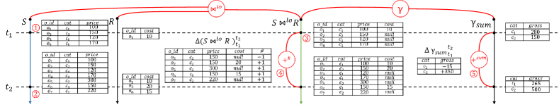
Figure 2: Example TVR’s and their relationships.

Definition 2

A time-varying relation (TVR) $R$ is a mapping from a time domain $\mathcal{T}$ to a bag of tuples belonging to a schema.

A snapshot of $R$ at a time $t$, denoted ${{R}_{t}}$, is the instance of $R$ at time $t$. For example, due to continuous ingestion, table Tablesales ($S$) in Example 1 is a TVR, depicted as the blue line in Fig. 2. On the line, tables ① and ② show the snapshots of $S$ at $t_{1}$ and $t_{2}$, i.e., ${{S}_{t_{1}}}$ and ${{S}_{t_{2}}}$, respectively. Traditional data warehouses run queries on relations at a specific time, while incremental execution runs queries on TVR’s.

Definition 3 (Querying TVR)

Given a TVR $R$ on time domain $\mathcal{T}$, applying a query $Q$ on $R$ defines another TVR $Q(R)$ on $\mathcal{T}$, where ${{[Q(R)]}_{t}}=Q({{R}_{t}}),\forall t\in\mathcal{T}$.

In other words, the snapshot of $Q(R)$ at $t$ is the same as applying $Q$ as a query on the snapshot of $R$ at $t$. For instance, in Fig. 2, joining two TVR’s Tablesales ($S$) and Tablereturns ($R$) yields a TVR $(S\bowtie^{lo}R)$, depicted as the green line. Snapshot ${{(S\bowtie^{lo}R)}_{t_{1}}}$ is shown as table ③, which is equal to joining ${{S}_{t_{1}}}$ and ${{R}_{t_{1}}}$. We denote left outer-join as $\bowtie^{lo}$, left anti-join as $\bowtie^{la}$, left semi-join as $\bowtie^{ls}$, and aggregate as $\gamma$. For brevity, we use “$Q$” to refer to the TVR “$Q(R)$” when there is no ambiguity.

3.2 Basic Operations on TVR’s

Besides as a sequence of snapshots, a TVR can be encoded from a delta perspective using the changes between two snapshots. We denote the difference between two snapshots of TVR $R$ at $t,t^{\prime}\in T$ ($t<t^{\prime}$) as the delta of $R$ from $t$ to $t^{\prime}$, denoted ${\Delta{R}_{t}^{t^{\prime}}}$, which defines a second-order TVR.

Definition 4 (TVR difference)

${\Delta{R}_{t}^{t^{\prime}}}$ defines a mapping from a time interval to a bag of tuples belonging to the same schema, such that there is a merge operator “$+$” satisfying ${{R}_{t}}+{\Delta{R}_{t}^{t^{\prime}}}={{R}_{t^{\prime}}}.$

Table ④ in Fig. 2 shows ${\Delta{(S\bowtie^{lo}R)}_{t_{1}}^{t_{2}}}$, which is the delta of snapshots ${{(S\bowtie^{lo}R)}_{t_{1}}}$ and ${{(S\bowtie^{lo}R)}_{t_{2}}}$. Here multiplicities $\#=+1/-1$ represent insertion and deletion of the corresponding tuple, respectively. The merge operator $+$ is defined as additive union on relations with bag semantics, which adds up the multiplicities of tuples in bags.

Interestingly, a TVR can have different snapshot/delta views. For instance, the delta ${\Delta{\gamma(S\bowtie^{lo}R)}_{t_{1}}^{t_{2}}}$ can be defined differently as Table ⑤ in Fig. 2. Here the merge operator $+$ directly sums up the partial SUM values (the gross attribute) per category. For category $c_{1}$, summing up the partial SUM’s in ${{\gamma(S\bowtie^{lo}R)}_{t_{1}}}$ and ${\Delta{\gamma(S\bowtie^{lo}R)}_{t_{1}}^{t_{2}}}$ yields the value in ${{\gamma(S\bowtie^{lo}R)}_{t_{2}}}$, i.e., $280+(-15)=265$. To differentiate these two merge operators, we denote the merge operator for $S\bowtie^{lo}R$ as $+^{\#}$, and the merge operator for $\gamma(S\bowtie^{lo}R)$ as $+^{sum}$.

This observation shows that the way to define TVR deltas and the merge operator $+$ is not unique. In general, as studied in previous research [32, 52], the difference between two snapshots ${{R}_{t}}$ and ${{R}_{t^{\prime}}}$ can have two types:

(1) Multiplicity Perspective. ${{R}_{t}}$ and ${{R}_{t^{\prime}}}$ may have different multiplicities of tuples. ${{R}_{t}}$ may have less or more tuples than ${{R}_{t^{\prime}}}$. In this case, the merge operator (e.g., $+^{\#}$) combines the same tuples by adding up their multiplicities.

(2) Attribute Perspective. ${{R}_{t}}$ may have different attribute values in some tuples compared to ${{R}_{t^{\prime}}}$. In this case, the merge operator (e.g., $+^{sum}$) groups tuples with the same primary key, and combines the delta updates on the changed attributes into one value. Aggregation operators usually produce this type of snapshots and deltas. Formally, distributed aggregation in data-parallel computing platforms is often modeled using four methods [51]:

1. Initialize: It is called once before any data is supplied with a given key to initialize the aggregate state.

2. Iterate: It is called every time a tuple is provided with a matching key to combine the tuple into the aggregate state.

3. Merge: It is called every time when combining two aggregate states with the same key into a single aggregate state.

4. Final: It is called at the end on the final aggregate state to produce a result.

For an aggregate function $\gamma$, the snapshots/deltas are the aggregate states computed using Initialize and Iterate on partial data; the merge operator $+^{\gamma}$ is defined using Merge; and at this end, the attribute-perspective snapshot is converted by Final to produce the multiplicity-perspective snapshot, i.e., the final result. For instance, for the aggregate function AVG, its snapshot/delta is an aggregate state consisting of a running SUM and COUNT on the partial data; the merge operator $+^{\texttt{AVG}}$ sums up the running SUM and COUNT, and at the end, the running SUM is divided by the running COUNT to get the final average. Note that for aggregates such as MEDIAN whose state needs to be the full set of tuples, Iterate and Merge degenerate to no-op.

Furthermore, for some merge operator $+$, there is an inverse operator $-$, such that ${{R}_{t^{\prime}}}-{{R}_{t}}={\Delta{R}_{t}^{t^{\prime}}}$. For instance, the inverse operator $-^{sum}$ for $+^{sum}$ is defined as taking the difference of SUM values per category between two snapshots.

4 TVR Rewrite Rules

Rewrite rules expressing relational algebra equivalence are the key mechanism that enables traditional query optimizers to explore the entire plan space. As TVR snapshots and deltas are simply static relations, traditional rewrite rules still hold within a single snapshot/delta. However, these rewrite rules are not enough for incremental query planning, due to their inability to express algebra equivalence between TVR concepts.

To capture this more general form of equivalence, in this section, we introduce TVR rewrite rules in the TIP model, focusing on logical plans. We propose a trichotomy of TVR rewrite rules, namely TVR-generating rules, intra-TVR rules, and inter-TVR rules, and show how to model existing incremental techniques using these three types of rules. This modeling enables us to unify existing incremental techniques and leverage them uniformly when exploring the plan space; it also allows IQP to evolve by adding new TVR rewrite rules.

4.1 TVR-Generating and Intra-TVR Rules

Most existing work on incremental computation revolves around the notion of delta query that can be described as Eq. 1 below.

$$Q({{R}_{t^{\prime}}})=Q({{R}_{t}}+{\Delta{R}_{t}^{t^{\prime}}})=Q({{R}_{t}})+\mathfrak{d}Q({{R}_{t}},{\Delta{R}_{t}^{t^{\prime}}}).$$ (1)

The idea is intuitive: when an input delta ${\Delta{R}_{t}^{t^{\prime}}}$ arrives, instead of recomputing the query on the new input snapshot ${{R}_{t^{\prime}}}$, one can directly compute a delta update to the previous query result $Q({{R}_{t}})$ using a new delta query $\mathfrak{d}Q$. Essentially, Eq. 1 contains two key parts—the delta query $\mathfrak{d}Q$ and the merge operator $+$, which correspond to the first two types of TVR rewrite rules, namely TVR-generating rules and intra-TVR rules, respectively.

TVR-Generating Rules. Formally, TVR-generating rules define for each relational operator on a TVR, how to compute its deltas from the snapshots and deltas of its input TVRs. In other words, TVR-generating rules define $\mathfrak{d}Q$ for each relational operator $Q$ such that ${\Delta{Q}_{t}^{t^{\prime}}}=\mathfrak{d}Q({{R}_{t}},{\Delta{R}_{t}^{t^{\prime}}})$. Many previous studies on deriving delta queries under different semantics [16, 17, 21, 26, 27] fall into this category. As an example, Fig. 3 shows the TVR-generating rules used by IM-1 in Example 1. The rules for left outer-join (Rule $(1)$) and aggregate (Rule $(2)$) are from [26] and [27], respectively. For simplicity, we separate the inserted/deleted part in a TVR delta, and denote them by superscripting $\Delta$ with $+/-$. The blue lines in Fig. 3 demonstrate these TVR-generating rules in a plan space.

Intra-TVR Rules. Intra-TVR rules define the conversion between the snapshots and deltas of a single TVR. As in Eq. 1, the merge operator $+$ defines how to merge $Q$’s snapshot ${{Q}_{t}}$ and delta ${\Delta{Q}_{t}^{t^{\prime}}}$ into a new snapshot ${{Q}_{t^{\prime}}}$. Other examples of intra-TVR rules include rules that merge deltas into a new delta, e.g., for a TVR $R$, ${\Delta{R}_{t}^{t^{\prime}}}+{\Delta{R}_{t^{\prime}}^{t^{\prime\prime}}}={\Delta{R}_{t}^{t^{\prime\prime}}}$, or rules that take the difference between snapshots/deltas if the merge operator $+$ has an inverse operator $-$, e.g., ${{R}_{t^{\prime}}}-{{R}_{t}}={\Delta{R}_{t}^{t^{\prime}}}$. The red lines in Fig. 3 demonstrate the intra-TVR rules used by IM-1 in Example 1. Note that when merging the snapshot/delta of $S\bowtie^{lo}R$ (subquery Tablesales_status), we use $+^{\#}$ (Rule $(3)$), whereas when merging the snapshot/delta of $\gamma(S\bowtie^{lo}R)$ (query Tablesummary), we use $+^{sum}$ ((Rule $(4)$).

4.2 Inter-TVR Rules

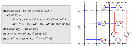
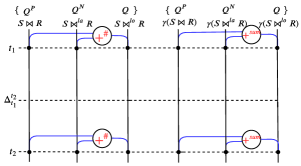
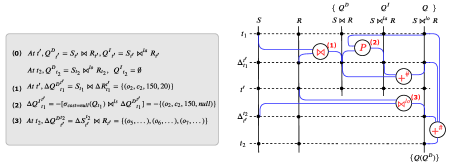
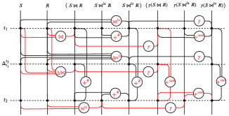
Figure 3: (a) Examples of TVR-generating and intra-TVR rules, (b) examples of inter-TVR equivalence rules in stream computing, (c) examples of inter-TVR equivalence rules in outer-join view maintenance, and (d) the incremental plan space of Example 1.

There are incremental techniques that cannot be modeled using the two aforementioned types rules alone. The IM-2 approach in Example 1 is such an example. Different from IM-1, approach IM-2 does not directly deliver the snapshot of $S\bowtie^{lo}R$ at $t_{1}$. Instead, it delivers only the subset of $S\bowtie^{lo}R$ that is guaranteed not to be retracted in the future, essentially the results of $S\bowtie R$. At $t_{2}$ when the data is known to be complete, IM-2 computes the rest part of $S\bowtie^{lo}R$, essentially $S\bowtie^{la}R$, then pads with nulls to match the output schema.

This observation shows another family of incremental techniques: without computing $Q$ directly, one can incrementally compute a set of different queries $\{Q^{\prime}_{1},\cdots,Q^{\prime}_{k}\}$, and then apply another query $P$ on their results to get that of $Q$, formally described as Eq. 2. The intuition is that $\{Q^{\prime}_{1},\cdots,Q^{\prime}_{k}\}$ may be more amenable to incremental computation and thus may be more efficient than directly incrementally computing $Q$:

$$Q(R)=P(Q^{\prime}_{1}(R),\cdots,Q^{\prime}_{k}(R)).$$ (2)

The family of techniques that Eq. 2 can describe are very general. They all rely on certain rewrite rules describing the equivalence between snapshots/deltas of multiple TVRs. We summarize this family of techniques into a third type of rules namely inter-TVR rules. Below we demonstrate using a couple of existing incremental techniques how they can be modeled by inter-TVR rules.

(1) The IM-2 approach: Let us revisit IM-2 using the terminology of inter-TVR rules. Formally, IM-2 decomposes $Q=S\bowtie^{lo}R$ into two parts, $Q^{P}$ and $Q^{N}$, defined below:

$${{Q^{P}}_{t}}={{S}_{t}}\bowtie{{R}_{t}} {{Q^{N}}_{t}}={{S}_{t}}\bowtie^{la}{{R}_{t}} {{Q}_{t}}={{Q^{P}}_{t}}+^{\#}{{Q^{N}}_{t}}$$ , , (3)

where $Q^{P}$ is a positive part that will not retract any tuple if both $S$ and $R$ are append-only, whereas $Q^{N}$ represents a part that could cause retractions at insertions to $S$ and $R$. The inter-TVR rule in Eq. 3 states that any snapshot of $Q$ can be decomposed into snapshots of $Q^{P}$ and $Q^{N}$ at the same time. Similar decomposition holds for the aggregate $\gamma$ in summary too, just with a different merge operator $+^{sum}$. Fig. 3 depicts these rules in a plan space. As it is much easier to incrementally compute inner join than left outer join, $Q^{P}$ can be incrementally computed using the TVR rewrite rules in §4.1 in a more efficient manner than $Q$, whereas $Q^{N}$ cannot be easily incrementalized, and is not computed until the completion time.

(2) Outer-join view maintenance: [33] proposed a method to incrementally maintain outer-join views. Its main idea can be summarized using two types of inter-TVR rules:

$${{Q}_{t}}={{Q^{D}}_{t}}+^{\#}{{Q^{I}}_{t}}+^{\#}{{Q^{U}}_{t}}$$ (4a) (4b)

The first type of rules described by Eq. 4a decompose a query into three parts given an update to a single input table: a directly affected part $Q^{D}$, an indirectly affected part $Q^{I}$, and an unaffected part $Q^{U}$, where $Q^{D}$, $Q^{I}$, and $Q^{U}$ are defined formally using the join-disjunctive normal form of $Q$. Due to space limitation we refer the readers to [33] for formal details. Intuitively, an insertion (deletion) into the input table will cause insertions (deletions) to $Q^{D}$ and deletions (insertions) to $Q^{I}$, but leave $Q^{U}$ unaffected. Eq. 4b describes the second type of rules that give a way to directly compute the deltas of $Q^{I}$ from the delta of $Q^{D}$ and the previous snapshot of $Q$. At updates, one can use the TVR-generating rules to compute the delta of $Q^{D}$, and the inter-TVR rules in Eq. 4b to get delta of $Q^{I}$, and these two deltas can be merged to incrementally compute $Q$, i.e., ${\Delta{Q}_{t}^{t^{\prime}}}={\Delta{Q^{D}}_{t}^{t^{\prime}}}+^{\#}{\Delta{Q^{I}}_{t}^{t^{\prime}}}$.

Take query Tablesales_status as an example. Fig. 3 shows the corresponding inter-TVR rules. As the algorithm in [33] considers updating one input table at a time, we insert a virtual time point $t^{\prime}$ between $t_{1}$ and $t_{2}$, assuming $R$ and $S$ are updated separately at $t^{\prime}$ and $t_{2}$. Rule $(0)$ shows the decomposition of Tablesales_status at $t^{\prime}$ and $t_{2}$ following the inter-TVR rule in Eq. 4a. By applying the TVR-generating rules, $Q^{D}$ can be incrementally computed as rules $(1)$ and $(3)$; whereas $Q^{I}$ can be incrementally computed following the inter-TVR rule in Eq. 4b, as shown in rule $(2)$. Combining them yields the delta of $Q$ as in Table ④ in Fig. 2.

(3) Higher-order view maintenance: [9, 38] proposed a higher-order view-maintenance algorithm, which can also be expressed by inter-TVR rules. The main idea is to treat the deltas of a query $Q$ as another TVR, and continue applying TVR rewrite rules to incrementally compute it. Formally, considering a query $Q$ and updates to one of its inputs $R$, the algorithm can be summarized as the following inter-TVR rule.

$${\Delta{Q}_{t}^{t^{\prime}}}=\mathfrak{d}Q({{R}_{t}},{\Delta{R}_{t}^{t^{\prime}}})=P({{M}_{t}},{\Delta{R}_{t}^{t^{\prime}}})$$ (5)

The rule decomposes the delta query into two parts: the delta update ${\Delta{R}_{t}^{t^{\prime}}}$, and an update-independent subquery $M$ that does not involve ${\Delta{R}_{t}^{t^{\prime}}}$. The two parts are combined using a query $P$ to get the delta of $Q$. If $M$ is a query involving input relations other than $R$, it can be further decomposed again with respect to updates to each of its input relations according to Eq. 5, until it becomes a constant. We refer the readers to [9] for a detailed algorithm. Take the Tablesummary query and updates to Tablesales ($S$) as an example (we denote Tablereturns as R). Applying Eq. 5, we can decompose it as

$${\Delta{Q}_{t}^{t^{\prime}}} =\gamma_{\textit{category};\texttt{SUM}(r)}({\Delta{S}_{t}^{t^{\prime}}}\bowtie^{lo}{{M}_{t}}),$$

$$\text{where~{}~{}~{}~{}}M_{t} =\gamma_{\textit{o\_id};\textit{total}=\texttt{SUM}(\textit{cost})}(\textit{R}_{t}),$$

$$r =\texttt{IF}(\textit{total}\texttt{ IS NULL},\textit{price},-\textit{total}).$$

$M$ essentially preprocesses Tablereturns by computing the total cost per o_id, and $P$ computes the gross revenue per category by summing up the precomputed total cost in $M$ or the prices of the new orders added to $S$. Then $M$ is materialized as a higher-order view and can be further incrementally maintained with respect to updates to Tablereturns by repeatedly applying the inter-TVR rule to generate higher-order views.

4.3 Putting Everything Together

The above concepts and observations lay a theoretical foundation for our IQP framework. Different TVR rules can be extended individually and can work with each other automatically. For example, TVR-generating rules can be applied on any TVR created by inter-TVR rules. By jointly applying TVR rewrite rules and traditional rewrite rules, we can explore a plan space much larger than that of any individual existing incremental method. For instance, if we overlay Fig. 3 and 3, we can achieve the plan space as shown in Fig. 3. Any tree rooted at ${{\gamma(S\bowtie^{lo}R)}_{t_{2}}}$ is a valid incremental plan for Example 1, e.g., the red lines indicate the plan used by IM-2.

In the next two sections, we discuss how to build an optimizer framework based on the TIP model, including plan-space exploration (§5) and selecting an optimal incremental plan (§6).

5 Plan-Space Exploration

In this section we study how Tempura explores the space of incremental plans. Existing query optimizers do the exploration only for a specific time. To support query optimization in incremental processing, we need to explore a much bigger plan space by considering not only relations at different times, but also transformations between them. We study how to extend existing query optimizers to support cost-based optimization for incremental processing based on the TIP model. As an example, we consider one of the state-of-the-art solutions, the Cascades-style cost-based optimizer [23, 25]. We illustrate how to incorporate the TIP model into such an optimization framework to develop the corresponding optimizer framework called Tempura.

Tempura consists of two main modules. (1) Memo: it keeps track of the explored plan space, i.e., all plan alternatives generated, in a succinct data structure, typically represented as an AND/OR tree, for detecting redundant derivations and fast retrieval. (2) Rule engine: it manages all the transformation rules, which specify algebraic equivalence laws and suitable physical implementations of logical operators, and monitors new plan alternatives generated in the memo. Whenever there are changes, the rule engine fires applicable transformation rules on the newly-generated plans to add more plan alternatives to the memo. The memo and rule engine of a traditional Cascades optimizer lack the capability to support IQP. We will focus on the key adaptations we made on the two modules to incorporate the TIP model.

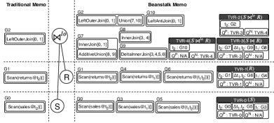
(a) An example memo of subquery Tablesales_status

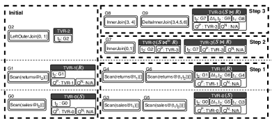
(b) A step-wise illustration of the growth of the memo

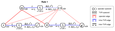
(c) A TVR-generating rule pattern

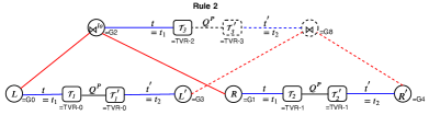
(d) An inter-TVR rule pattern

Figure 4: Examples of the memo and TVR rewrite-rule patterns in Tempura.

5.1 Memo: Capturing TVR Relationships

The memo in the traditional Cascades-style optimizer only captures two levels of equivalence relationship: logical equivalence and physical equivalence. A logical equivalence class groups operators that generate the same result set; within each logical equivalence class, operators are further grouped into physical equivalence classes by their physical properties such as sort order, distribution, etc. The “Traditional Memo” part in Fig. 4(a) depicts the traditional memo of the Tablesales_status query. For brevity, we omit the physical equivalence classes. For instance, LeftOuterJoin[0,1] has Groups G0 and G1 as children, and it corresponds to the plan tree rooted at $\bowtie^{lo}$. G2 represents all plans logically equivalent to LeftOuterJoin[0,1].

However, the above two equivalences are not enough to capture the rich relationships along the time dimension and between different incremental computation methods in the TIP model. For example, the relationship between snapshots and deltas of a TVR cannot be modeled using the logical equivalence due to the following reasons. Two snapshots at different times produce different relations, and the snapshots and deltas do not even have the same schema (deltas have an extra $\#$ column). To solve this problem, on top of logical/physical equivalence classes, we explicitly introduce TVR nodes into the memo, and keep track of the following relationships, shown as the “Tempura Memo” part in Fig. 4(a).

• Intra-TVR relationship specifies the snapshot/delta relationship between logical equivalence classes of operators and the corresponding TVR’s. For example, the traditional memo only models scanning the full content of $S$, i.e., ${{S}_{t_{2}}}$, represented by G0, while the Tempura memo models two more scans: scanning the partial content of $S$ available at $t_{1}$ (${{S}_{t_{1}}}$), and scanning the delta input of $S$ newly available at $t_{2}$ (${\Delta{S}_{t_{1}}^{t_{2}}}$). These two new scans are represented by G3 and G5, and the memo uses an explicit TVR-0 to keep track of these intra-TVR relationships.

• Inter-TVR relationship specifies the user-defined relationship between TVR’s introduced by inter-TVR equivalence rules. For example, the IM-2 approach decomposes TVR-2 ($S\bowtie^{lo}R$) into two parts $Q^{P}$ and $Q^{N}$ as discussed in §3, represented by TVR-3 and TVR-4, respectively. It is worth noting that the above relationships are transitive. For instance, as G7 is the snapshot at $t_{2}$ of TVR-3 and TVR-3 is the $Q^{P}$ part of TVR-2, it is the snapshot at $t_{2}$ of the $Q^{P}$ part of TVR-2.

5.2 Rule Engine: Enabling TVR Rewritings

As the memo of Tempura strictly subsumes a traditional Cascades memo, traditional rewrite rules can be adopted and work without modifications. Besides, the rule engine of Tempura supports TVR rewrite rules. Tempura allows optimizer developers to define TVR rewrite rules by specifying a graph pattern on both relational operators and TVR nodes in the memo. A TVR rewrite rule pattern consists of two types of nodes and three types of edges: (1) operator operands that match relational operators; (2) TVR operands that match TVR nodes; (3) operator edges between operator operands that specify traditional parent-child relationship of operators; (4) intra-TVR edges between operator operands and TVR operands that specify intra-TVR relationships; and (5) inter-TVR edges between TVR operands that specify inter-TVR relationships. All nodes and intra/inter-TVR edges can have predicates. Once fired, TVR rewrite rules can register new TVR nodes and intra/inter-TVR relationships.

Fig. 4(c)-4(d) depict two TVR rewrite rules, where solid nodes and edges specify the patterns to match, and dotted ones are newly registered by the rules. In the figures, we also show an example match of these rules when applied on the memo in Fig. 4(a):

• Rule 1 is the TVR-generating rule for computing the delta of an inner join. It matches a snapshot of an InnerJoin, whose children $L$ ($R$) have a delta sibling $L^{\prime}$ ($R^{\prime}$) respectively. The rule will generate a DeltaInnerJoin taking $L$, $R$, $L^{\prime}$, and $R^{\prime}$ as inputs, and register it as a delta sibling of the original InnerJoin.

• Rule 2 is an inter-TVR rule of IM-2. The rule matches a snapshot of a LeftOuterJoin, whose children $L$, $R$ each have a $Q^{P}$ snapshot sibling $L^{\prime}$, $R^{\prime}$. The rule will generate an InnerJoin of $L^{\prime}$ and $R^{\prime}$, and register it as the $Q^{P}$ snapshot sibling of the original LeftOuterJoin.

Fig. 4(b) demonstrates the growth of a memo in Tempura. For each step, we only draw the updated part due to space limitation. The memo starts with G0 to G2 and their corresponding TVR-0 to TVR-2. In step 1, we first populate the snapshots and deltas of the scan operators, e.g., G3 to G6, and register the intra-TVR relationship in TVR-0 and TVR-1. We also populate their $Q^{P}$ and $Q^{N}$ inter-TVR relationships as in IM-2 (for base tables these relationships are trivial). In step 2, rule 2 fires on the tree rooted at LeftOuterJoin[0,1] in G2 as in Fig. 4(d). In step 3, rule 1 fires on the tree rooted at InnerJoin[0,1] in G7 as in Fig. 4(c). Similarly by applying other TVR rewrite rules, we can eventually populate the memo in Fig. 4(a).

5.3 Implementation

Next we explain the implementation details of Tempura, based on the terminology of Apache Calcite 1.17.0 [3].

Apache Calcite uses RelSet and RelSubset to represent the logical and physical equivalence classes, respectively, and Trait to represent the physical properties of a physical equivalence class. On top of that, Tempura introduces TvrMetaSet to represent the TVRs, as well as IntraTvrTrait and InterTvrTrait to represent the intra-TVR and inter-TVR relationship respectively. Each intra-TVR/inter-TVR relationship is recorded in the involved TVRs and operators. E.g., an intra-TVR relationship is modeled as a triple $\langle\texttt{TvrMetaSet},\texttt{IntraTvrTrait},\texttt{RelSet}\rangle$ and stored in the corresponding TvrMetaSet and RelSet. We allow users to define their own IntraTvrTrait’s and InterTvrTrait’s, and also implement several commonly-used ones as in §3. For instance, the attribute-perspective IntraTvrTrait for the group-by aggregate operator consists of the group-by keys (the primary keys of the aggregate results), and the merge operator $+^{\gamma}$ for each aggregate column $\gamma$. The InterTvrTrait for the IM-2 approach comprises of an indicator whether it is the $Q^{P}$ or $Q^{N}$ part.

To facilitate fast rule triggering, Tempura indexes the rule patterns by their containing operator operands and intra/inter-TVR edges. Similar to Calcite, Tempura monitors new structural changes in the memo. Whenever new operators or intra/inter-TVR relationships are registered in the memo, Tempura only fires the rule patterns that contain operator operands or intra/inter-TVR edges that match the changes. Note that we do not index the TVR operands and the operator edges, as they do not have predicates to facilitate filtering.

Initially, the rule engine starts with registering the original logical plan, and associates each RelSet to a TvrMetaSet with a default IntraTvrTrait. When a traditional rule is fired on a set of operators, if the RelSet of every matched operator is already connected to a TvrMetaSet via the default IntraTvrTrait, then besides registering the new operators generated by the rule, Tempura also creates a new TvrMetaSet for each new operator and connects them with the default IntraTvrTrait. In general, all structural changes in the memo will cause rules to match and fire, and further generate new nodes and edges. Tempura does not distinguish TVR rules from traditional rules in terms of rule firing. All rule matches are stored in the same queue, and the firing order is determined by the customizable scoring function. We used the default Calcite scoring function, which takes into consideration the rule importance and the location of the matched relation operators in the memo. We adjusted the scoring function for TVR rules by giving them a boosting factor, because TVR rules are transformations on logical plans and we want them to be fired with higher priorities. Similar to Calcite, Tempura deduplicates the TVRs besides the operators when registering them in the memo. Two TVRs are considered equivalent if they are both connected to a RelSet with the same default IntraTvrTrait.

5.4 Speeding Up Exploration Process

In this section, we discuss optimizations to speed up the exploration process, which is needed since IQP explores a much bigger plan space than traditional query planning.

Translational symmetry of TVR’s. The structures in the Tempura memo usually have translation symmetry along the timeline, because the same rule generates similar patterns when applied on snapshots or deltas of the same set of TVR’s. For instance, in Fig. 4(d), if we let $t^{\prime}=t_{1}$ instead, $L^{\prime}$ ($R^{\prime}$) will match G0 (G1) instead of G3 (G4), and we will generate the InnerJoin in G7 instead of G8. In other words, InnerJoin[0,1] in G7 and InnerJoin[3,4] are translation symmetric, modulo the fact that G0, G1, and G7 (G3, G4, and G8) are all snapshot $t_{1}$ ($t_{2}$) of the corresponding TVR’s respectively.

By leveraging this symmetry, instead of repeatedly firing TVR rewrite rules on snapshots/deltas of the same set of TVR’s, we can apply the rules on just one snapshot/delta, and copy the structures to other snapshots/deltas. This helps eliminate the expensive repetitive matching process of the same rule patterns on the memo. The improved process is as follows:

1. We seed the TVR’s of the leaf operators (usually Scan) with only one snapshot plus a consecutive delta, and fire all the rewrite rules to populate the memo.

2. We seed the TVR’s leaf operators with all snapshots and deltas, and copy the memo from step 1 by substituting its leaf operators with their snapshot/delta siblings in the corresponding TVR’s.

3. We continue optimizing the copied memo, as we can further apply time-specific optimization, e.g., pruning empty relations if a delta at a specific time is empty.

Pruning non-promising alternatives. There are multiple ways to compute a TVR’s snapshot or delta, within which certain ways are usually more costly than others. We can prune the non-promising alternatives. For instance, to compute a delta, one can take the difference of two snapshots, or use TVR-generating rules to directly compute from deltas of the inputs. Based on the experience of previous research on incremental computation [31], we know that the plans generated by TVR-generating rules are usually more efficient. Therefore, for operators that are known to be easily incrementally maintained, such as filter and project, we assign a lower importance to intra-TVR rules for generating deltas to defer their firing. Once we find a delta that can be generated through TVR-generating rules, we skip the corresponding intra-TVR rules altogether. To implement this optimization, we can give this subset of intra-TVR rules a lower priority than all other rules, and thus other TVR rewrite rules and traditional rewrite rules will always be ranked higher. Each intra-TVR rule also has an extra skipping condition, which is tested to see whether the target delta is already generated before firing the rule. If so, the rule is skipped.

Guided exploration. Inside a TVR, snapshots and deltas consecutive in time can be merged together, leading to combinatorial explosion of rule applications. However, the merge order of these snapshots and deltas usually do not affect the cost of the final plan. Thus, we limit the exploration to a left-deep merge order. Specifically, we disable merging of consecutive deltas, but instead only let rules match patterns that merge a snapshot with its immediately consecutive delta. In this way, we always use a left-deep merge order.

6 Selecting an Optimal Plan

In this section we discuss how Tempura selects an optimal incremental plan in the explored space. The problem has two distinctions from existing query optimization: (1) costing the plan space and searching through the space need to consider the temporal execution of a plan; and (2) the optimal plan needs to decide which states to materialize to maximize the sharing opportunities between different time points within a query.

6.1 Time-Point Annotations of Operators

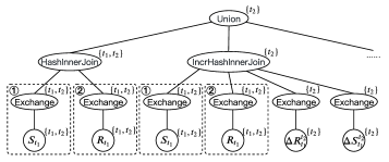
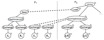
Figure 5: Examples of (a) the temporal plan space, and (b) an temporal assignment of the physical plan for subquery Tablesales_status.

Costing the plan alternatives properly is crucial for correct optimization. However, as the temporal dimension is involved in query planning, costing is not trivial. Fig. 5 depicts one physical plan alternative derived from the plan rooted at ${{(S\bowtie^{lo}R)}_{t_{2}}}$ shown in red in Fig. 3. This plan only specifies the concrete physical operations taken on the data, but does not specify when these physical operations are executed. Actually, each operator in the plan usually has multiple choices of execution time. In Fig. 5, the time points annotated alongside each operator shows the possible temporal domain in which each operator can be executed. For instance, snapshots ${{S}_{t_{1}}}$ and ${{R}_{t_{1}}}$ are available at $t_{1}$, and thus can execute at any time after that, i.e., $t_{1}$ or $t_{2}$. Deltas ${\Delta{R}_{t_{1}}^{t_{2}}}$ and ${\Delta{S}_{t_{1}}^{t_{2}}}$ are not available until $t_{2}$, and thus any operators taking it as input, including the IncrHashInnerJoin, can only be executed at $t_{2}$. The temporal domain of each operator $O$, denoted $\text{t-dom}(O)$, can be defined inductively:

• For a base relation $R$, $\text{t-dom}(R)$ is the set of execution times that are no earlier than the time point when $R$ is available.

• For an operator $O$ with inputs $I_{1},\ldots,I_{k}$, $\text{t-dom}(R)$ is the intersection of its inputs’ temporal domains: $\text{t-dom}(R)$ $=$ $\cap_{1\leq j\leq k}{\text{t-dom}(I_{j})}$.

To fully describe a physical plan, one has to assign each operator in the plan an execution time from the corresponding temporal domain. We denote a specific execution time of an operator $O$ as $\tau(O)$. We have the following definition of a valid temporal assignment.

Definition 5 (Valid Temporal Assignment)

An assignment of execution times to a physical plan is valid if and only if for each operator $O$, its execution time $\tau(O)$ satisfies $\tau(O)\in\text{t-dom}(O)$ and $\tau(O)\geq\tau(O^{\prime})$ for all operators $O^{\prime}$ in the subtree rooted at $O$.

Fig. 5 demonstrates a valid temporal assignment of the physical plan in Fig. 5. As ${{S}_{t_{1}}}$ and ${{R}_{t_{1}}}$ are already available at $t_{1}$, the plan chooses to compute HashInnerJoin of ${{S}_{t_{1}}}$ and ${{R}_{t_{1}}}$ at $t_{1}$, as well as shuffling ${{S}_{t_{1}}}$ and ${{R}_{t_{1}}}$ in order to prepare for IncrHashInnerJoin. At $t_{2}$, the plan shuffles the new deltas ${\Delta{S}_{t_{1}}^{t_{2}}}$ and ${\Delta{R}_{t_{1}}^{t_{2}}}$, finishes IncrHashInnerJoin, and unions the results with that of HashInnerJoin computed at $t_{1}$. Note that if an operator $O$ and its input $I$ have different execution times, then the output of $I$ needs to be saved first at $\tau(I)$, and later loaded and fed into $O$ at $\tau(O)$, e.g., Union at $t_{2}$ and HashInnerJoin at $t_{1}$. The cost of Save and Load needs to be properly included in the plan cost. It is worth noting that some operators save and load the output as a by-product, for which we can spare Save and Load, e.g., Exchange of ${{S}_{t_{1}}},{{R}_{t_{1}}}$ at $t_{1}$ for IncrHashInnerJoin.

6.2 Time-Point-Based Cost Functions

The cost of an incremental plan is defined under a specific assignment of execution times. Therefore, the optimization problem of searching for the optimal incremental plan is formulated as: given a plan space, find a physical plan and temporal assignment that achieve the lowest cost. In this section, we discuss the cost model and optimization algorithm for this problem without considering sharing common sub-plans. We will discuss the problem of how to decide the optimal sharable sub-plans to materialize in §6.3.

As an incremental plan can span across multiple time points, the cost function $\tilde{\mathfrak{c}}$ in an IQP problem (as in §2.1) is extended to a function taking into consideration of costs at different times. For the cost at each time point, we inherit the general cost model used in traditional query optimizers, i.e., the cost of a plan is the sum of the costs of all its operators. Below we give two examples of $\tilde{\mathfrak{c}}$. We denote traditional cost functions as $c$, and $c_{i}$ is the cost at time $t_{i}$. As before, $c$ can be a number, e.g., estimated monetized resource cost, or a structure, e.g., a vector of CPU time and I/O.

1. $\tilde{c}_{w}(O)=\sum_{i=1..T}{w_{i}\cdot c_{i}(O)}$. That is, the extended cost of an operator is a weighted sum of its cost at each time $t_{i}$. For the example setting in §2.2, $w_{1}=0.2$ for $t_{1}$ and $w_{2}=1$ for $t_{2}$.

2. $\tilde{c}_{v}(O)=[c_{1}(O),\ldots,c_{T}(O)]$. That is, the extended cost is a vector combining costs at different times. $\tilde{c}_{v}$ can be compared entry-wise in a reverse lexical order. Formally, $\tilde{c}_{v}(O_{1})>\tilde{c}_{v}(O_{2})$ iff $\exists j$ s.t. $c_{j}(O_{1})>c_{j}(O_{2})$ and $c_{i}(O_{1})=c_{i}(O_{2})$ for all $i,j<i\leq T$.

Consider the plan in Fig. 5 as an example. To get the result of HashInnerJoin at $t_{2}$, we have two options: (i) compute the join at $t_{2}$; or (ii) as in Fig. 5, compute the join at $t_{1}$, save the result, and load it back at $t_{2}$. Assume the cost of computing HashInnerJoin, saving the result, and loading it are $10$, $5$, $4$, respectively. Then for option (i) $(c_{1},c_{2})=(0,10)$, for option (ii) $(c_{1},c_{2})=(15,4)$. Say that we use $\tilde{c}_{w}$ as the cost function. If $w_{1}=0.6$ and $w_{2}=1$ then option (i) is better, whereas if $w_{1}=0.2$ and $w_{2}=1$, option (ii) becomes better.

Dynamic programming used predominantly in existing query optimizers [42, 35, 25] also need to be adapted to handle the cost model extensions. In these existing query optimizers, the state space of the dynamic programming is the set of all operators in the plan space, represented as $\{O\}$. Each operator $O$ records the best cost of all the subtrees rooted at $O$. We extend the state space by considering all combinations of operators and their execution times, i.e., $\{O\}\times\text{t-dom}(\{O\})$. Also instead of recording a single optimum, each operator $O$ records multiple optimums, one for each execution time $\tau(O)$, which represents the best cost of all the subtrees rooted at $O$ if $O$ is generated at $\tau$. During optimization, the state-transition function is as Eq. 6. That is, the best cost of $O$ if executed at $\tau$ is the best cost of all possible plans of computing $O$ with all possible valid temporal assignments compatible with $\tau$.

$$\tilde{\mathfrak{c}}[O,\tau]=min_{\forall\text{ valid }\tau_{j}}\bigl{(}\sum_{j}\tilde{\mathfrak{c}}[I_{j},\tau_{j}]+c_{\tau}(O)\bigr{)}.$$ (6)

In general, we can apply dynamic programming to the optimization problem for any cost function satisfying the property of optimal substructure. We have the following correctness result of the above dynamic programming algorithm.

Theorem 6

The optimization problem under cost functions $\tilde{c}_{w}$ and $\tilde{c}_{v}$ without sharing common sub-plans satisfies the property of optimal substructure, and dynamic programming is applicable.

6.3 Deciding States to Materialize

The problem of deciding the states to materialize can be modeled as finding the sharing opportunities in the plan space. In other words, a shared sub-plan between $P_{i}$ and $P_{j}$ in an incremental plan is essentially an intermediate state that can be saved by $P_{i}$ and reused by $P_{j}$. For example, in Fig. 5, since both HashInnerJoin and IncrHashInnerJoin require shuffling ${{S}_{t_{1}}}$ and ${{R}_{t_{1}}}$, the two relations can be shuffled only once and reused for both joins. The parts ① and② circled in dashed lines depict the sharable sub-plans.

Finding the optimal common sub-plans to share is a multi-query optimization (MQO) problem, which has been extensively studied [40, 54, 30]. In this paper, we extend the MQO algorithm in [30], which proposes a greedy framework on top of Cascade-style optimizers for MQO. For the sake of completeness, we list the algorithm in Algo. 1, by highlighting the extensions for progressive planning. The algorithm runs in an iterative fashion. In each iteration, it picks one more candidate from all possible shareable candidates, which if materialized can minimize the plan cost (line 4), where $bestPlan(\mathbb{S})$ means the best plan with $\mathbb{S}$ materialized and shared. The algorithm terminates when all candidates are considered or adding candidates can no longer improve the plan cost. As IQP needs to consider the temporal dimension, the shareable candidates are no longer solely the set of shareable sub-plans, but pairs of a shareable sub-plan $s$ and a choice of its execution time $\tau(s)$. Pair $\langle s,\tau(s)\rangle$ means computing and materializing the sub-plan $s$ at time $\tau(s)$, which can only benefit the computation that happens after $\tau(s)$. For instance, considering the physical plan space in Fig. 5, the sharable candidates are $\{\langle\text{①},t_{1}\rangle,\langle\text{①},t_{2}\rangle,\langle\text{②},t_{1}\rangle,\langle\text{②},t_{2}\rangle\}$. The optimizations in [30] are still applicable to Algo. 1.

1:  $\mathbb{S}=\emptyset$

2:  $\mathbb{C}=$ shareable candidate set consiting of all shareable nodes and their potential execution times $\{\langle s,\tau(s)\rangle\}$

3:  while $\mathbb{C}\neq\emptyset$ do

4:      Pick $\langle s,\tau(s)\rangle\in\mathbb{C}$ that minimizes $\tilde{\mathfrak{c}}(bestPlan(\mathbb{S}^{\prime}))$ where $\mathbb{S}^{\prime}=\{\langle s,\tau(s)\rangle\}\cup\mathbb{S}$

5:      if $\tilde{\mathfrak{c}}(bestPlan(\mathbb{S}^{\prime}))<\tilde{\mathfrak{c}}(bestPlan(\mathbb{S}^{\prime}))$ then

6:           $\mathbb{C}=\mathbb{C}-\{\langle s,\tau(s)\rangle\}$

7:           $\mathbb{S}=\mathbb{S}^{\prime}$

8:      else

9:           $\mathbb{C}=\emptyset$

10:  return  $\mathbb{S}$

Algorithm 1 Greedy Algorithm for MQO

As expanded with execution time options, the enumeration space of the shareable candidate set becomes much larger than the original algorithm in [30]. Interestingly, we find that under certain cost models we can reduce the enumeration space down to a size comparable to the original algorithm, formally summarized in Theorem 7. This theorem relies on the fact that materializing a shareable sub-plan at its earliest possible time subsumes other materialization choices. Due to space limit, we omit the proof.

Theorem 7

For a cost function $\tilde{c}_{w}$ satisfying $w_{i}<w_{j}$ if $i<j$, or a cost function $\tilde{c}_{v}$ satisfying the property that an entry $i$ has a lower priority than an entry $j$ if $i<j$ in the lexical order, we only need to consider the earliest valid execution time for each shareable sub-plan. That is, for each shareable sub-plan $s$, we only need to consider the shareable candidate $\langle s,min(\text{t-dom}(s))\rangle$ in Algorithm 1.

7 Beanstalk in Action

In this section, we discuss a few important considerations when applying Tempura in practice.

Dynamic Re-optimization of incremental plans. We have studied the IQP problem assuming a static setting, i.e., in $(\vec{T},\vec{D},\vec{Q},\tilde{\mathfrak{c}})$ where $\vec{T}$ and $\vec{D}$ are given and fixed. In many cases, the setting can be much more dynamic where $\vec{T}$ and $\vec{D}$ are subject to change. Fortunately, Tempura can be adapted to a dynamic setting using re-optimization. Generally, an incremental plan $\mathbb{P}{}=[P_{1},\cdots,P_{i-1},P_{i},$ $\cdots,P_{k}]$ for $\vec{T}=[t_{1},\cdots,t_{i-1},t_{i},\cdots,t_{k}]$ is only executed up to $t_{i-1}$, after which $\vec{T}$ and $\vec{D}$ change to $\vec{T^{\prime}}=[t_{i^{\prime}},\cdots,t_{k^{\prime}}]$ and $\vec{D^{\prime}}=[D_{i^{\prime}},\cdots,D_{k^{\prime}}]$. Tempura can adapt to this change by re-optimizing the plan under $\vec{T^{\prime}}$ and $\vec{D^{\prime}}$. We want to remark that during re-optimization, Tempura can incorporate the materialized states generated by $P_{1},\cdots,P_{i-1}$ as materialized views. In this way Tempura can choose to reuse the materialized states instead of blindly recomputing everything.

Take the progressive data warehouse scenario as an example. Since we may not know the exact schedule and data statistics in the future, we do not optimize for a large number of time points at once. Instead, one can plan adaptively using re-optimization. Consider a query originally scheduled at $t^{*}$. Say, initially at $t_{1}$ we decide to have one incremental run. At this planning stage, we only need to consider a simple schedule $[t_{1},t^{*}]$. In the resulting plan $[P_{1},P^{*}]$, only $P_{1}$ is executed, but co-planing $P_{1},P^{*}$ makes $P_{1}$ robust for future runs. At a future time $t_{i}$, if we decide to have another run, we can always re-optimize for $[t_{i},t^{*}]$ with accurate statistics for $t_{i}$ (as data is already available). We can also take into consideration the materialized states from previous runs before $t_{i}$. Note that at each planning, we only optimize a small IQP problem with a limited number of time points. This way, we avoid planning many time points with uncertain schedule and statistics. The above methods are used in [48].

Data statistics estimation. Incremental processing scenarios usually involve planning for logical times or physical times in the future, for which estimating the data statistics becomes very challenging. IQP scenarios, including both planning for logical times (e.g., IVM-PD) and physical times (e.g., PWD-PD) as described in §2.1, usually involve recurring queries. Thus, we can use historical data’s arrival patterns to estimate the statistics of available data at logical time points or physical time points in the future. Having inaccurate statistics is not a new problem to query optimization, and many techniques have been proposed [50] to tackle this issue. Note that we can always re-optimize the plan when we find that the previously estimated statistics is not accurate. Also, techniques such as robust planning [13, 24, 49] and parametric planning [28] can be adopted to IQP too. It is out of the scope of this paper.

8 Experiments

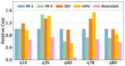
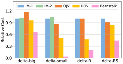
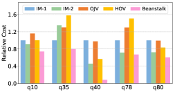
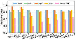
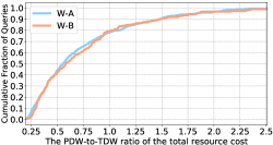
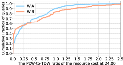
Figure 6: (a)(b) The optimal estimated costs of different incremental plans in IVM-PD for different queries and data-arrival patterns. (c)(d) The optimal estimated costs of different incremental plans in PDW-PD for different queries, data-arrival patterns and cost weights. (e)(f) The PDW-to-TDW ratio of the real total CPU cost and CPU cost at $24$:$00$ for the data warehouse workloads respectively.

In this section, we report our experimental study on the effectiveness and efficiency of Tempura in IQP.

8.1 Settings

We used the query optimizer of Alibaba Cloud MaxCompute [1], which was built on Apache Calcite 1.17.0 [3], as a traditional optimizer baseline. We implemented Tempura on the optimizer of MaxCompute. We integrated four commonly used incremental methods into Tempura by expressing them as TVR-rewrite rules: (1) IM-1: as described in §2.2. (2) IM-2: as described in §2.2 and §4.2. (3) OJV: the outer-join view maintenance algorithm in §4.2. (4) HOV: the higher-order view maintenance algorithm in §4.2. By default, Tempura jointly considered all four methods to generate an optimal plan. In the experiments, we used Tempura to simulate each method by turning off the inter-TVR rules of the other methods.

Incremental Processing Scenarios. We used two incremental processing scenarios to demonstrate Tempura. Below are the incremental planning problem definitions for these two scenarios.

• Progressive data warehouse. We use the PDW-PD definition as in §2.2. Specifically, We used $\tilde{c}_{w}(O)$ (in §6.2) as the cost function, where the cost at each time $c_{i}$ was a linear combination of the estimated usage of CPU, IO, memory, and network transfer, and the weight $w_{i}\in[0.25,0.3]$ for early runs and $w_{i}=1$ for the last run. Note that it helped us achieve a balance between re-computation and the size of materialized states by jointly considering CPU and memory in the cost function. We chose $w_{i}\leq 0.3$ for early runs to simulate the tiered rates of resources on Amazon AWS [2], where spot instances usually cost less than $30\%$ of on-demand instances.

• Incremental view Maintenance. We use the IVM-PD definition as defined in §2.1.

Query Workloads. We used the TPC-DS benchmark [6] ($1TB$) to study the effectiveness (§8.2) and performance (§8.4) of Tempura. To further demonstrate the effectiveness of the incremental plans produced by Tempura, in §8.3, we used two real-world analysis workloads consisting of recurrent daily jobs from Alibaba’s enterprise progressive data warehouse, denoted as W-A and W-B. Table 1 shows statistics of the two workloads.

Table 1: Statistics of two workloads at Alibaba

	# Queries	Avg. # Joins	# with $\geq 1$ join	# with $\geq 2$ joins
W-A	$274$	$1.14$	$167$	$83$
W-B	$554$	$1.18$	$357$	$144$

Running Environment. In the experiments, query optimization was carried out single-threaded on a machine with an Intel Xeon Platinum $8163$ CPU @ $2.50$GHz and $512$GB memory, whereas the generated query was executed on a cluster of thousands of machines shared with other production workloads.

8.2 Effectiveness of IQP

We first evaluated the effectiveness of IQP by comparing Tempura with four individual incremental methods IM-1, IM-2, OJV, and HOV, in both the PDW-PD and IVM-PD scenarios. We controlled and varied two factors in the experiments: (1) Queries. We chose five representative queries covering complex joins (inner-, left-outer-, and left-semi-joins) and aggregates. (2) Data-arrival patterns. We controlled the amount of input data available in the 1st and 2nd incremental runs ($D_{1},D_{2}$) and whether there are retractions in the input data. Correspondingly, we chose the following four data-arrival patterns, namely delta-big ($|D_{1}|/|D_{2}|=1:1$), delta-small ($|D_{1}|/|D_{2}|=4:1$), delta-R ($|D_{1}|/|D_{2}|=2:1$ with retractions in the Tablesales tables), and delta-RS ($|D_{1}|/|D_{2}|=2:1$ with retractions in both Tablesales and Tablereturns tables). As the accuracy of cost estimation is orthogonal to Tempura, to isolate its interference, we mainly compared the estimated costs of plans produced by the optimizer, and reported them in relative scale (dividing them by the corresponding costs of IM-1) for easy comparison. We reported the real execution costs as a reference later. Due to space limit, we only report the most significant entries in the cost vector of $\tilde{c}_{v}$ for IVM-PD.

IVM-PD. We first fixed the data-arrival pattern to delta-big and varied the queries. The optimal-plan costs are reported in Fig. 6. As shown, different queries prefer different incremental methods. For example, IM-1 outperformed both OJV and HOV for complex queries such as q35. This is because OJV computed $Q^{I}$ by left-semi joining the delta of $Q^{D}$ with the previous snapshot (§4.2), and a bigger delta incurred a higher cost of computing $Q^{I}$. Whereas for simpler queries such as q80, OJV degenerated to a similar plan as IM-1, and thus had similar costs. Note that HOV cost much less than both OJV and IM-1. This is because HOV maintained extra higher-order views (e.g., Tablecatalog_sales inner joining with Tablewarehouse, Tableitem and Tabledate_dim) and thus avoided repeated recomputation of these views as in OJV and IM-1. Tempura outperformed the individual incremental methods on all queries. The reason is that Tempura was able to combine the benefits of different incremental methods.

Next we chose query q10 as a complex query with multiple left outer joins, and varied the data-arrival patterns. The results are plotted in Fig. 6. Again, the data-arrival patterns affected the preference of incremental methods. For example, IM-2 could not handle input data with retractions. Compared to delta-big, HOV started to outperform IM-1 by a large margin in delta-small, as both of them could use different join orders when applying updates to different input relations, and a smaller delta help significantly reduce the cost of incrementally computing $M$ in HOV and $Q^{D},Q^{I}$ in OJV.

For both experiments, Tempura consistently delivered the best plans among all the methods. For example, for q40 in Fig. 6 and the delta-small case in Fig. 6, Tempura delivered a plan $5$-$10$X better than others. Tempura leveraged all three of HOV, IM-2 and IM-1 to generate a mixed optimal plan: Tempura chose different join orders when applying updates to different input relations, which was similar to HOV. It leveraged the fact that joining the smaller delta earlier can quickly reduce the output sizes. Interestingly, when it came to combining higher-order views $M$ and $\Delta R$ as required by HOV, Tempura used the IM-2 approach, and applied IM-1 to incrementally compute the $Q^{N}$ part in IM-2.

PDW-PD. For the PDW-PD scenario, we conducted the same experiments by varying the queries and the data-arrival patterns as in IVM-PD, and in addition tried different weights used in the cost functions ($w_{1}=0.3$ vs. $w_{1}=0.7$). We reported the results in Figures 6 and 6. We have similar conclusions as in IVM-PD. We make two remarks. (1) Since the PDW-PD setting did not require any outputs at earlier runs, Tempura automatically avoided unnecessary computation, e.g., computing the $Q^{N}$ part in an IM-2 approach, which usually cannot be efficiently incrementally maintained. This result is also shown in the figures, as the IM-2 approach was more preferred uniformly in PDW-PD than in IVM-PD. (2) The weights in the cost function can also affect the choice of the optimizer. For instance, in Fig. 6, q10 preferred HOV to OJV when $w_{1}=0.3$, but the other way when $w_{1}=0.7$. This result was because as the cost of early execution became higher, it was less preferable to store many intermediate states as in HOV. Tempura automatically exploited this fact and adjusted the amount of computation in each incremental run. When $w_{1}$ increased from $0.3$ to $0.7$, Tempura moved some early computation from the first incremental run to the second.

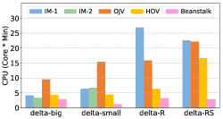
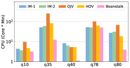
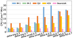
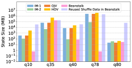
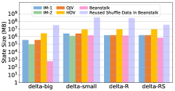
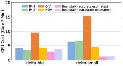
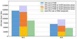
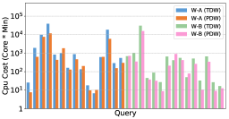
Figure 7: (a)(b) The optimal real CPU costs of different incremental plans in IVM-PD for different queries and data-arrival patterns. (c)(d) The optimal real CPU costs of different incremental plans in PDW-PD for different queries, data-arrival patterns and cost weights. (e)(f) The state sizes of different incremental plans in IVM-PD for different queries and data-arrival patterns. (g) The plan quality of Tempura under inaccurate cardinality estimation. (h) The comparison between TDW and PDW on the CPU cost breakdowns of all queries in W-A and W-B, and (i) a detailed comparison of $30$ randomly sampled queries in W-A and W-B.

Real CPU Costs. We reported the real CPU costs (in the unit of CPU$\cdot$minute) in Fig. 7-7 for the experiments in Fig. 6-6. In the PDW-PD experiments (Fig. 7 and 7), the CPU costs were weighted according to the cost function in PWD-PD. Note that Fig. 7 and 7 are plotted in log scale due to the huge differences in CPU costs for different queries. As we can see, the real CPU costs were agreed with the planner’s estimation (Fig. 6-6) pretty well. Some of the real costs were different from the estimated ones because of the inaccuracy of the cost model. But note that Tempura consistently delivered the best plans with the lowest CPU consumption across all experiments.

State Sizes. In this set of experiments, we study the storage costs of materialized states between Tempura and each individual incremental methods. We first fixed the data-arrival pattern to delta-big and tested different queries under IVM-PD settings respectively. The results are reported in Fig. 7. As shown, for most queries, the sizes of states materialized by Tempura were smaller than or comparable to each individual incremental algorithms. This is due to the fact that Tempura is able to reuse the shuffled data as the states without incurring additional storage overheads (see §6.1). Thus, we further reported the sizes of the shuffled data reused by Tempura in the figures. Next we chose query q10 and varied the data-arrival patterns. The results are reported in Fig. 7. Again, the storage costs of Tempura were lower than or comparable to that of each individual incremental algorithms.

Sensitivity to Inaccurate Estimates. Next, we evaluated the sensitivity of Tempura to inaccurate cardinality estimation. To set up the experiment, we used q10 in the IVM-PD scenario. We gave Tempura the estimation of delta-small when running q10 with input delta-big, and gave the estimation of delta-big when running q10 with input delta-small. Fig. 7 reported the real CPU costs. For delta-big, Tempura with the inaccurate estimation ran slower compared to Tempura with accurate estimation. This is expected because Tempura chose a plan that is optimal to the inaccurate cost model. Nevertheless, Tempura was still faster than IM-1, OJV, HOV, and comparable to IM-2. For delta-small, inaccurate estimation had a small impact on execution time, and Tempura was still faster than each individual incremental method.

Remarks. In conclusion, the optimal incremental plan is affected by different factors and does need to be searched in a principled cost-based way, and Tempura can consistently find better plans than each incremental method alone.

8.3 Case Study: Progressive Data Warehouse

To validate the effectiveness of Tempura in a real application, we conducted a case study of the PDW-PD scenario using two real-world analysis workloads W-A and W-B at Alibaba. We compared the resource usage of executing these workloads in a traditional data warehouse and a progressive one: (1) Traditional (TDW), where we ran the analysis workloads at $24$:$00$ according to a schedule using the plans generated by a traditional optimizer; and (2) Progressive (PDW), where besides $24$:$00$, we also early executed the analysis workloads at $14$:$00$ and $19$:$00$ with only partial data using the incremental plans generated by Tempura. The two early-execution time points were chosen to simulate the observed cluster usage pattern (the cluster was often under-utilized at these times), for which we set the weights of resource cost to $0.25$ and $0.3$, respectively.

Fig. 6 shows the real CPU cost of executing the workloads (scored using the cost function in the PDW-PD setting), where we plotted the cumulative distribution of the ratio between the CPU cost in PDW versus that in TDW. We can see that PDW delivered better CPU cost for $80\%$ of the queries. For about $60\%$ of the queries, PDW was able to cut the CPU cost by more than $35\%$. Remarkably, PDW delivered a total cost reduction of $56.2\%$ and $55.5\%$ for W-A and W-B, respectively. Note that Tempura searched plans based on the estimated costs which could be different from the real execution cost. As a consequence, for some of the queries (less than $10\%$) we see more than $50\%$ cost increase. Accuracy of cost estimation is not within the scope of the paper. We further reported the PDW-to-TDW ratio of the CPU cost at $24$:$00$ in Fig. 6, as this ratio indicated the resource reduction during the “rush hours.” As shown, for both workloads, PDW reduced the resource usage at peak hours for over $85\%$ of the queries, and for over $70\%$ of the queries we can see significant reduction of more than $25\%$.

We also reported the absolute values of CPU costs of W-A and W-B. However, as W-A and W-B have $274$ and $554$ queries each, it is not realistic to show all of them. Instead we reported the total CPU cost breakdowns for TDW and PDW in Fig. 7. Specifically for PDW, we reported the absolute values of CPU costs at each time, and the total CPU costs weighted according to the cost function in PDW-PD. As we can see, Tempura indeed picked better plans with less resource consumption: PDW saved $38.7\%$ and $32.6\%$ CPU costs compared to TDW for W-A and W-B respectively. On the other hand, with incremental computation, PDW brought relatively low overheads compared to TDW, $19.6\%$ and $37.6\%$ for W-A and W-B respectively. The PDW overheads are computed by summing up the absolute values of CPU costs at each time, minus the CPU costs of TDW. We further randomly selected $15$ queries from W-A and W-B respectively, and reported their CPU costs in TDW and PDW in Fig. 7. Again, for most queries PDW reduced the CPU costs by a significant amount.

8.4 Performance of IQP

Next, we evaluated the time performance of Tempura in IQP. Compared to traditional query planning, IQP has two salient characteristics: (1) In plan-space exploration, IQP explores a larger plan space. (2) Besides, IQP needs to decide the intermediate states to share, which are not considered by traditional query planning. We will present performance results on these two phases: Plan-Space Exploration (PSE) and State Materialization Optimization (SMO).

We used PDW-PD as the IQP problem definition. Unless otherwise specified, in the problem definition we set $|\vec{T}|=3$. To help readers better understand how Tempura performs on different types of queries, we use the TPC-DS queries, and present the optimization time of Tempura on them. Besides the overall performance study, we also present a detailed study on four aspects of Tempura’s optimization performance:

Table 2: Statistics of selected representative queries

Query	Q22	Q20	Q43	Q67	Q27	Q99	Q85	Q91	Q5	Q33
# Joins	2	2	2	3	4	4	6	6	7	9
# Agg-
regates	1	1	1	1	1	1	1	1	4	4
# Sub-
Queries	0	0	0	2	0	0	0	0	7	7

1. Query complexity: How does Tempura perform when queries become increasingly complex, e.g., with more joins or subqueries?

2. Size of IQP: How does Tempura perform when the number of incremental runs (i.e., $|\vec{T}|$) in the IQP problem definition changes?

3. Number of incremental methods: How does Tempura perform when users integrate more incremental methods into it?

4. Optimization breakdown: How effective are the speed-up optimizations discussed in §5.4?

To study the above four aspects, we further selected ten representative TPC-DS queries with different numbers of joins, aggregates, and subqueries. The selected queries are shown in Table 2.

Overall Planning Performance. We first studied the overall query planning performance by comparing IQP with traditional planning. Fig. 8 shows the end-to-end planning time on all TPC-DS queries. As shown, although IQP planned a much bigger plan space than traditional planning, Tempura still delivered high planning performance: IQP finished within $3$ seconds for $80\%$ queries, and for all queries finished within $14$ seconds. For over $80\%$ queries, the IQP optimization time was less than $24$X of the traditional planning time. Even though slower than traditional planning at optimization time on a single machine, IQP generated much better incremental plans that brought significant benefit in resource usage and query latency on a cluster. We can further reduce the planning time by adopting a parallel optimizer [43]. As a reference, we also reported the real CPU cost used by TDW, the CPU costs saved by PDW compared to TDW, and the planning time in Fig. 9. We can see that for most queries, the CPU time on planning was $2$-$3$ orders of magnitude smaller than the saved CPU costs. This shows that the planning cost is negligible compared to the execution cost. Thus the benefit of a better plan outweighs the extra time spent on planning.

Query Complexity. To study the impact of query complexity on performance, we tested on the selected TPC-DS queriesin Table 2, and reported the broken-down optimization times in Fig. 8. As one can see, the planning time increased slowly when the query complexity increased, because the plan space grew larger for complex queries. The time spent on PSE was less than that spent on SMO in general, and also grew with a slower pace. This result shows that query complexity has a smaller impact on PSE.

Size of IQP. To study the impact of the size of the planning problem on the planning time, we gradually increased the number of incremental runs planned from $3$ to $9$, and reported the time on PSE and SMO in Fig. 8 and 8. As depicted, the time on PSE stayed almost constant as the size of IQP changed. E.g., when the number of incremental runs grew $3$X, the time for q$33$ only slightly increased by $20\%$. This was mainly due to the effective speed-up optimization techniques introduced in §5.4. In comparison, the SMO time increased superlinearly with increasing number of incremental runs, due to the time complexity of the MQO algorithm we chose [30].

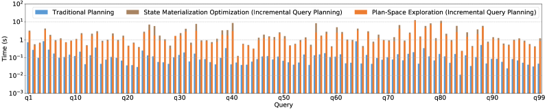
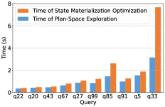
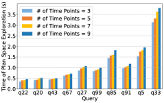
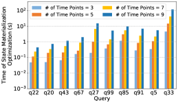
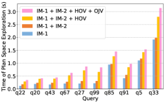
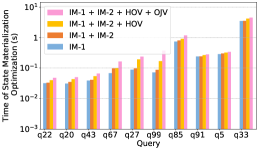
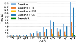
Figure 8: (a) Overall planning performance comparison on the TPC-DS benchmark between traditional and incremental query planning. (b) Impact of the query complexity on the planning performance. (c) (d) Impact of the planning problem size on the planning performance. (e)(f) Impact of the number of incremental methods on the planning performance. (g) Effectiveness of the speed-up optimization techniques. Note that the selected queries are ordered by their query complexity(as listed in Table 2).

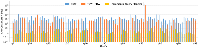
Figure 9: Real resource consumption of Tempura’s plan as in Fig. 8 on 1T TPC-DS benchmark.

Number of Incremental Methods. Next, we evaluated how the performance scales when more incremental methods are added into the optimizer by gradually adding methods IM-1, IM-2, HOV and OJV into Tempura. Fig. 8 and 8 show the time on PSE and SMO, respectively. As illustrated, the time on both PSE and SMO increased when more incremental methods were added, because more incremental methods increased the plan space. There are two interesting findings. (1) The PSE time did not grow linearly with the number of incremental methods, but rather the size of the plan space that each method newly introduces. For example, the difference of PSE time introduced by adding HOV was bigger than that introduced by adding OJV. This was because HOV and OJV use similar methods that update a single relation at a time, which are very different from IM-1 and IM-2 that update all relations each time. (2) The number of incremental methods had less impact on the planning time than the size of the IQP problem, which can be observed on the SMO time. This is mainly because the plan space explored by different incremental methods often have overlaps, e.g., most incremental methods fundamentally share similar delta update rules as IM-1, whereas the plan spaces of different incremental runs do not have overlaps.

Optimization Breakdown. In the end, we evaluated the effectiveness of the speed-up optimizations by breaking down the optimization techniques discussed in §5.4, i.e., translational symmetry (TS), pruning non-promising alternatives (PNA), and guided exploration (GE). Fig. 8 reports the PSE times of different combinations of the speed-up optimizations. We compared the implementations with no optimization (Baseline), with each individual optimization (Baseline+TS, Baseline+PNA, Baseline+GE), and with all three optimizations (Tempura). As shown, the optimizations together brought an order of magnitude performance improvements. The most effective optimizations were PNA and TS. PNA generally improved the PSE time by $5$-$12$X, while TS improved the PSE time by $1.5$-$2.5$X.

9 Related Work

Incremental Processing. There is a rich body of research on various forms of incremental processing, ranging from incremental view maintenance, stream computing, to approximate query answering and so on. Incremental view maintenance has been intensively studied before. It has been considered under both the set [16, 17] and bag [21, 27] semantics, for queries with outer joins [26, 33], and using higher-order maintenance methods [9]. Previous studies mainly focused on delta propagation rules for relational operators. Stream computing [7, 22, 37, 46] adopts incremental processing and sublinear-space algorithms to process updates and deltas. Many approximate query answering studies [8, 12, 20] focused on constructing optimal samples to improve query accuracy. Proactive or trigger-based incremental computation techniques [52, 19] were used to achieve low query latency. Zeng et al. [52] proposed a probability-based pruning technique for incrementally computing complex queries including those with nested queries. These studies proposed incremental computation techniques in isolation, and do not have a general cost-based optimization framework, which is the focus of this paper. In addition, they can be integrated into Tempura, and contribute to a unified plan space for searching the optimal incremental plan.

Query Planning for Incremental Processing. Previous work studied some optimization problems in incremental computation. Viglas et al. [47] proposed a rate-based cost model for stream processing. The cost model is orthogonal to Tempura and can be integrated. DBToaster [9] discussed a cost-based approach to deciding the views to materialize under a higher-order view maintenance algorithm. Tang et al. [44] focused on selecting optimal states to materialize for scenarios with intermittent data arrival. They proposed a dynamic programming algorithm for selecting intermediate states to materialize given a fixed physical incremental plan and a memory budget, by considering future data-arrival patterns. These optimization techniques all focus on the optimal materialization problem for a specific incremental plan or incremental method, and thus are not general IQP solutions.

Flink [4] uses Calcite [15] as the optimizer and support stream queries, which only provides traditional optimizations on the logical plan generated by a fixed incremental method, but cannot explore the plan space of multiple incremental methods, nor consider correlations between incremental runs. On the contrary, Tempura provides a general framework for users to integrate various incremental methods, and searches the plan space in a cost-based approach.

Semantic Models for Incremental Processing. CQL[11] exploited the relational model to provide strong query semantics for stream processing. Sax et al. [41] introduced the Dual Streaming Model to reason about ordering in stream processing. The key idea behind [11, 41] is the duality of relations and streams, i.e., time-varying relations can be modeled as a sequence of static relations, or a sequence of change logs consisting of INSERT and DELETE operations. The recent work [14] proposed to integrate streaming into the SQL standard, and briefly mentioned that TVR’s can serve as a unified basis of both relations and streams. However, their models do not include a formal algebra and rewrite rules on TVR’s, and thus cannot fully model incremental computation. To the best of our knowledge, our TIP model for the first time formally defines an algebra on TVR’s, especially it provides a principled way to model different types of snapshot/deltas in multiplicity/attribute perspectives and $+/-$ operators between them. Furthermore, the TIP model provides a trichotomy of all TVR rewrite rules and shows that the three types of rewrite rules can subsume many existing incremental algorithms, which provides a theoretical foundation for Tempura, so that Tempura can implement all incremental algorithms that can be described using the three types of TVR rewrite rules.

10 Conclusion

In this paper, we developed a novel, principled cost-based optimizer framework, called Tempura, for optimizing incremental data processing. We first proposed a theory called TIP model as its foundation, which can formally model incremental processing in its most general form. We gave a full specification of Tempura, which can not only unify various existing techniques to generate an optimal incremental plan, but also allow the developer to add their rewrite rules. We studied how to explore the plan space and search for an optimal incremental plan. We conducted thorough experimental evaluation of Tempura in various incremental-query scenarios to show its effectiveness and efficiency.

References

- [1] Alibaba Cloud MaxCompute. https://www.alibabacloud.com/product/maxcompute.
- [2] Amazon spot instance pricing history. https://docs.aws.amazon.com/AWSEC2/latest/UserGuide/using-spot-instances-history.html.
- [3] Apache Calcite. https://calcite.apache.org.
- [4] Apache Flink. https://flink.apache.org.
- [5] Introducing Stream-Stream Joins in Apache Spark 2.3. https://databricks.com/blog/2018/03/13/introducing-stream-stream-joins-in-apache-spark-2-3.html.
- [6] The TPC-DS Benchmark. http://www.tpc.org/tpcds/.
- [7] D. J. Abadi, Y. Ahmad, M. Balazinska, U. Cetintemel, M. Cherniack, J.-H. Hwang, W. Lindner, A. Maskey, A. Rasin, E. Ryvkina, et al. The design of the borealis stream processing engine. In Cidr, volume 5, pages 277–289, 2005.
- [8] S. Acharya, P. B. Gibbons, V. Poosala, and S. Ramaswamy. The aqua approximate query answering system. In ACM Sigmod Record, volume 28, pages 574–576. ACM, 1999.
- [9] Y. Ahmad, O. Kennedy, C. Koch, and M. Nikolic. Dbtoaster: Higher-order delta processing for dynamic, frequently fresh views. PVLDB, 5(10):968–979, 2012.
- [10] A. Aiken, J. M. Hellerstein, and J. Widom. Static analysis techniques for predicting the behavior of active database rules. ACM Transactions on Database Systems (TODS), 20(1):3–41, 1995.
- [11] A. Arasu, S. Babu, and J. Widom. The cql continuous query language: semantic foundations and query execution. The VLDB Journal, 15(2):121–142, 2006.
- [12] B. Babcock, S. Chaudhuri, and G. Das. Dynamic sample selection for approximate query processing. In Proceedings of the 2003 ACM SIGMOD international conference on Management of data, pages 539–550. ACM, 2003.
- [13] S. Babu, P. Bizarro, and D. DeWitt. Proactive re-optimization. In Proceedings of the 2005 ACM SIGMOD international conference on Management of data, pages 107–118, 2005.
- [14] E. Begoli, T. Akidau, F. Hueske, J. Hyde, K. Knight, and K. Knowles. One SQL to rule them all. CoRR, abs/1905.12133, 2019.
- [15] E. Begoli, J. Camacho-Rodríguez, J. Hyde, M. J. Mior, and D. Lemire. Apache calcite: A foundational framework for optimized query processing over heterogeneous data sources. In Proceedings of the 2018 International Conference on Management of Data, SIGMOD ’18, pages 221–230, New York, NY, USA, 2018. ACM.
- [16] J. A. Blakeley, P.-A. Larson, and F. W. Tompa. Efficiently updating materialized views. In Proceedings of the 1986 ACM SIGMOD International Conference on Management of Data, SIGMOD ’86, pages 61–71, New York, NY, USA, 1986. ACM.
- [17] O. P. Buneman and E. K. Clemons. Efficiently monitoring relational databases. ACM Trans. Database Syst., 4(3):368–382, Sept. 1979.
- [18] B. Chandramouli, C. N. Bond, S. Babu, and J. Yang. Query suspend and resume. In Proceedings of the 2007 ACM SIGMOD international conference on Management of data, pages 557–568, 2007.
- [19] B. Chandramouli, J. Goldstein, and A. Quamar. Scalable progressive analytics on big data in the cloud. Proc. VLDB Endow., 6(14):1726–1737, Sept. 2013.
- [20] S. Chaudhuri, G. Das, and V. Narasayya. Optimized stratified sampling for approximate query processing. ACM Transactions on Database Systems (TODS), 32(2):9, 2007.
- [21] S. Chaudhuri, R. Krishnamurthy, S. Potamianos, and K. Shim. Optimizing queries with materialized views. In Proceedings of the Eleventh International Conference on Data Engineering, ICDE ’95, pages 190–200, Washington, DC, USA, 1995. IEEE Computer Society.
- [22] T. M. Ghanem, A. K. Elmagarmid, P.-Å. Larson, and W. G. Aref. Supporting views in data stream management systems. ACM Transactions on Database Systems (TODS), 35(1):1, 2010.
- [23] G. Graefe. The cascades framework for query optimization. Data Engineering Bulletin, 18, 1995.
- [24] G. Graefe, W. Guy, H. A. Kuno, and G. Paullley. Robust query processing (dagstuhl seminar 12321). In Dagstuhl Reports, volume 2. Schloss Dagstuhl-Leibniz-Zentrum fuer Informatik, 2012.
- [25] G. Graefe and W. J. McKenna. The volcano optimizer generator: Extensibility and efficient search. In Proceedings of IEEE 9th International Conference on Data Engineering, pages 209–218. IEEE.
- [26] T. Griffin and B. Kumar. Algebraic change propagation for semijoin and outerjoin queries. SIGMOD Rec., 27(3):22–27, Sept. 1998.
- [27] T. Griffin and L. Libkin. Incremental maintenance of views with duplicates. In Proceedings of the 1995 ACM SIGMOD International Conference on Management of Data, SIGMOD ’95, pages 328–339, New York, NY, USA, 1995. ACM.
- [28] Y. E. Ioannidis, R. T. Ng, K. Shim, and T. K. Sellis. Parametric query optimization. The VLDB Journal, 6(2):132–151, 1997.
- [29] J. Jia, C. Li, and M. J. Carey. Drum: A rhythmic approach to interactive analytics on large data. In 2017 IEEE International Conference on Big Data (Big Data), pages 636–645. IEEE, 2017.
- [30] T. Kathuria and S. Sudarshan. Efficient and provable multi-query optimization. In Proceedings of the 36th ACM SIGMOD-SIGACT-SIGAI Symposium on Principles of Database Systems, PODS ’17, pages 53–67, New York, NY, USA, 2017. ACM.
- [31] C. Koch. Incremental query evaluation in a ring of databases. In Proceedings of the twenty-ninth ACM SIGMOD-SIGACT-SIGART symposium on Principles of database systems, pages 87–98, 2010.
- [32] W. Lang, R. V. Nehme, E. Robinson, and J. F. Naughton. Partial results in database systems. In Proceedings of the 2014 ACM SIGMOD International Conference on Management of Data, SIGMOD ’14, pages 1275–1286, New York, NY, USA, 2014. ACM.
- [33] P. Larson and J. Zhou. Efficient maintenance of materialized outer-join views. In Proceedings of the 23rd International Conference on Data Engineering, ICDE 2007, The Marmara Hotel, Istanbul, Turkey, April 15-20, 2007, pages 56–65, 2007.
- [34] Y.-N. Law, H. Wang, and C. Zaniolo. Query languages and data models for database sequences and data streams. In Proceedings of the Thirtieth International Conference on Very Large Data Bases - Volume 30, VLDB ’04, page 492–503. VLDB Endowment, 2004.
- [35] M. K. Lee. Implementing an interpreter for functional rules in a query optimizer. 1988.
- [36] D. Maier, J. Li, P. Tucker, K. Tufte, and V. Papadimos. Semantics of data streams and operators. In T. Eiter and L. Libkin, editors, Database Theory - ICDT 2005, pages 37–52, Berlin, Heidelberg, 2005. Springer Berlin Heidelberg.
- [37] R. Motwani, J. Widom, A. Arasu, B. Babcock, S. Babu, M. Datar, G. Manku, C. Olston, J. Rosenstein, and R. Varma. Query processing, resource management, and approximation in a data stream management system. CIDR, 2003.
- [38] M. Nikolic, M. Dashti, and C. Koch. How to win a hot dog eating contest: Distributed incremental view maintenance with batch updates. In Proceedings of the 2016 International Conference on Management of Data, SIGMOD ’16, pages 511–526, New York, NY, USA, 2016. ACM.
- [39] V. Raman and J. M. Hellerstein. Partial results for online query processing. In Proceedings of the 2002 ACM SIGMOD international conference on Management of data, pages 275–286, 2002.
- [40] P. Roy, S. Seshadri, S. Sudarshan, and S. Bhobe. Efficient and extensible algorithms for multi query optimization. In Proceedings of the 2000 ACM SIGMOD International Conference on Management of Data, SIGMOD ’00, pages 249–260, New York, NY, USA, 2000. ACM.
- [41] M. J. Sax, G. Wang, M. Weidlich, and J.-C. Freytag. Streams and tables: Two sides of the same coin. In Proceedings of the International Workshop on Real-Time Business Intelligence and Analytics, BIRTE ’18, New York, NY, USA, 2018. Association for Computing Machinery.
- [42] P. G. Selinger, M. M. Astrahan, D. D. Chamberlin, R. A. Lorie, and T. G. Price. Access path selection in a relational database management system. In Proceedings of the 1979 ACM SIGMOD international conference on Management of data, pages 23–34, 1979.
- [43] M. A. Soliman, L. Antova, V. Raghavan, A. El-Helw, Z. Gu, E. Shen, G. C. Caragea, C. Garcia-Alvarado, F. Rahman, M. Petropoulos, F. Waas, S. Narayanan, K. Krikellas, and R. Baldwin. Orca: A modular query optimizer architecture for big data. In Proceedings of the 2014 ACM SIGMOD International Conference on Management of Data, SIGMOD ’14, pages 337–348, New York, NY, USA, 2014. ACM.
- [44] D. Tang, Z. Shang, A. J. Elmore, S. Krishnan, and M. J. Franklin. Intermittent query processing. Proc. VLDB Endow., 12(11):1427–1441, July 2019.
- [45] D. Terry, D. Goldberg, D. Nichols, and B. Oki. Continuous queries over append-only databases. In Proceedings of the 1992 ACM SIGMOD International Conference on Management of Data, SIGMOD ’92, page 321–330, New York, NY, USA, 1992. Association for Computing Machinery.
- [46] H. Thakkar, N. Laptev, H. Mousavi, B. Mozafari, V. Russo, and C. Zaniolo. Smm: A data stream management system for knowledge discovery. In 2011 IEEE 27th International Conference on Data Engineering, pages 757–768. IEEE, 2011.
- [47] S. D. Viglas and J. F. Naughton. Rate-based query optimization for streaming information sources. In Proceedings of the 2002 ACM SIGMOD international conference on Management of data, pages 37–48, 2002.
- [48] Z. Wang, K. Zeng, B. Huang, W. Chen, X. Cui, B. Wang, J. Liu, L. Fan, D. Qu, Z. Ho, T. Guan, C. Li, and J. Zhou. Grosbeak: A data warehouse supporting resource-aware incremental computing. In Proceedings of the 2020 ACM SIGMOD International Conference on Management of Data, SIGMOD ’20, Portland, Oregon, USA, 2020. ACM.
- [49] F. Wolf, N. May, P. R. Willems, and K.-U. Sattler. On the calculation of optimality ranges for relational query execution plans. In Proceedings of the 2018 International Conference on Management of Data, SIGMOD ’18, page 663–675, New York, NY, USA, 2018. Association for Computing Machinery.
- [50] S. Yin, A. Hameurlain, and F. Morvan. Robust query optimization methods with respect to estimation errors: A survey. ACM Sigmod Record, 44(3):25–36, 2015.
- [51] Y. Yu, P. K. Gunda, and M. Isard. Distributed aggregation for data-parallel computing: interfaces and implementations. In Proceedings of the ACM SIGOPS 22nd symposium on Operating systems principles, pages 247–260, 2009.
- [52] K. Zeng, S. Agarwal, and I. Stoica. iolap: Managing uncertainty for efficient incremental olap. In Proceedings of the 2016 International Conference on Management of Data, SIGMOD ’16, pages 1347–1361, New York, NY, USA, 2016. ACM.
- [53] Y. Zhang, B. Hull, H. Balakrishnan, and S. Madden. Icedb: Intermittently-connected continuous query processing. In 2007 IEEE 23rd International Conference on Data Engineering, pages 166–175. IEEE, 2007.
- [54] J. Zhou, P.-A. Larson, P.-A. Larson, J.-C. Freytag, and W. Lehner. Efficient exploitation of similar subexpressions for query processing. In Proceedings of the 2007 ACM SIGMOD International Conference on Management of Data, SIGMOD ’07, pages 533–544, New York, NY, USA, 2007. ACM.