Recursive CSI Quantization of Time-Correlated MIMO Channels by Deep Learning Classification

Abstract

In frequency division duplex (FDD) multiple-input multiple-output (MIMO) wireless communications, limited channel state information (CSI) feedback is a central tool to support advanced single- and multi-user MIMO beamforming/precoding. To achieve a given CSI quality, the CSI quantization codebook size has to grow exponentially with the number of antennas, leading to quantization complexity, as well as, feedback overhead issues for larger MIMO systems. We have recently proposed a multi-stage recursive Grassmannian quantizer that enables a significant complexity reduction of CSI quantization. In this paper, we show that this recursive quantizer can effectively be combined with deep learning classification to further reduce the complexity, and that it can exploit temporal channel correlations to reduce the CSI feedback overhead.

I Introduction

Limited CSI feedback is a well-established technique for supporting efficient MIMO transmissions in FDD systems [1, 2, 3, 4]. Often, the framework of Grassmannian CSI quantization is adopted, since subspace information is required for many popular transmit precoding schemes. A large number of different ways for constructing Grassmannian quantization codebooks exists; e.g., [5, 6, 7, 8] to mention just a few of the more recent constructions.

Generally, in case of memoryless quantization of isotropic channels, such as, independent and identically distributed (i.i.d.) Rayleigh fading channels, it is known that maximally spaced subspace packings achieve optimal quantization performance in terms of subspace chordal distance; however, such packings are difficult to construct for larger MIMO systems and codebook sizes [9, 10, 11]. When adopting Grassmannian quantization in larger-scale MIMO systems and/or for high resolution quantization, one faces two main challenges: 1) quantization complexity and 2) feedback overhead. The former issue can effectively be tackled, if the channel exhibits structure that can be exploited for quantization; e.g., in the millimeter wave band, the channel is often assumed to be sparse, which allows for efficient parametric CSI quantization by sparse decomposition [12, 13, 14]. Such techniques, however, are not applicable in i.i.d. Rayleigh fading situations. Also, recently, a number of approaches that utilize deep neural networks have been proposed to enable efficient CSI quantization [15, 16, 17]; yet, these publications mostly consider relatively low resolution quantization, as neural networks are hard to train for large quantization codebooks. When the channel exhibits temporal correlation, quantizers with memory, such as, differential quantizers or techniques based on recurrent neural networks, can provide significantly better performance than memoryless approaches [18, 19, 20, 21, 22, 23, 24, 25]. Yet, they mostly require adaptation of the quantization codebook on the fly or online neural network learning, which can be prohibitive in terms of complexity.

Contribution: In [26], we have proposed a recursive multi-stage quantization approach that can reduce the complexity of high resolution Grassmannian quantization in moderate to large-scale MIMO systems by orders of magnitude. In this paper, we show that this approach can effectively be enhanced by DNN classification to further reduce the implementation complexity and, thus, support high resolution Grassmannian quantization with low complexity. Hence, rather than adopting an end-to-end DNN approach, we propose to enhance well-known model-based CSI quantizers by neural network features. We furthermore propose a simple approach to exploit temporal channel correlation in recursive multi-stage quantization, by selectively updating the individual stages of the quantizer.

Notation: The Grassmann manifold of $m$-dimensional subspaces of the $n$-dimensional Euclidean space is $\mathcal{G}\left(n,m\right)$. The trace of matrix $\mathbf{A}$ is $\mathrm{tr}\left(\mathbf{A}\right)$, the conjugate-transpose is $\mathbf{A}^{\mathsf{H}}$, the Frobenius norm is $\left\|\mathbf{A}\right\|$ and vectorization is $\mathrm{vec}\left(\mathbf{A}\right)$. The $m$-dimensional subspace spanned by the columns of $\mathbf{A}\in\mathbb{C}^{n\times m}$, $m\leq n$ is $\mathrm{span}\left(\mathbf{A}\right)$. The expected value of random variable $x$ is $\mathbb{E}\left(x\right)$. The operation $a_{\text{min}}=\operatornamewithlimits{arg\,min}_{a\in\mathcal{A}}f(a)$ determines the minimizer $a_{\text{min}}$ of the function $f(a)$ over the set $\mathcal{A}$. The size of set $\mathcal{A}$ is $\left|\mathcal{A}\right|$. The vector-valued complex Gaussian distribution with mean $\bm{\mu}$ and covariance $\mathbf{C}$ is $\mathcal{CN}\left(\bm{\mu},\mathbf{C}\right)$. The zeroth-order Bessel function of the first kind is $J_{0}(\cdot)$.

II Channel Model

We consider a MIMO wireless communication system with $n$ transmit- and $m$ receive-antennas, where $n>m$. We denote the frequency-flat baseband MIMO channel matrix at time instant $k$ as $\mathbf{H}[k]\in\mathbb{C}^{n\times m}$. We consider a spatially uncorrelated Rayleigh fading channel, i.e., $\mathrm{vec}\left(\mathbf{H}[k]\right)\sim\mathcal{CN}\left(\mathbf{0},\mathbf{I}_{nm}\right)$, as caused by a strong scattering environment.

We assume that the MIMO channel follows a stationary Gaussian stochastic process with temporal auto-correlation function parametrized by the time-lag $\Delta k$ according to

$$\bm{\Gamma}[\Delta k]=\mathbb{E}\left(\mathrm{vec}\left(\mathbf{H}[k]\right)\left(\mathrm{vec}\left(\mathbf{H}[k+\Delta k]\right)\right)^{\mathsf{H}}\right).$$ (1)

Considering, for example, Clarke’s Doppler spectrum [27], the auto-correlation function is $\bm{\Gamma}[\Delta k]=J_{0}\left(2\pi\nu_{d}\Delta k\right)\mathbf{I}_{nm}$, where $\nu_{d}=f_{d}T_{s}$ is the normalized Doppler shift, $f_{d}$ is the maximal absolute Doppler shift and $T_{s}$ is the symbol time interval.

III Grassmannian Quantization

In this paper, we focus on Grassmannian CSI quantization at the receiver, in order to provide CSI feedback to the transmitter. For this purpose, we apply a compact size singular value decomposition (SVD) to the channel

$$\mathbf{H}[k]=\mathbf{U}[k]\bm{\Sigma}[k]\mathbf{V}[k]^{\mathsf{H}},$$ (2)

and utilize the orthogonal basis $\mathbf{U}[k]\in\mathbb{C}^{n\times m}$, consisting of the left singular vectors corresponding to the non-zero singular values, as relevant CSI to represent the $m$-dimensional subspace spanned by the channel $\mathrm{span}\left(\mathbf{H}[k]\right)=\mathrm{span}\left(\mathbf{U}[k]\right)$.

III-A Single-Stage Quantization

In single-stage quantization, matrix $\mathbf{U}[k]$ is quantized by applying a quantization codebook $\mathcal{Q}_{m}^{n}[k]$ consisting of semi-unitary matrices $\mathbf{Q}\in\mathbb{C}^{n\times m}$, $\mathbf{Q}^{\mathsf{H}}\mathbf{Q}=\mathbf{I}_{m}$. For $b$ bits of CSI feedback per time instant, the codebook is of size $\left|\mathcal{Q}_{m}^{n}[k]\right|=2^{b}$.

As quantization metric, we consider the subspace chordal distance, as it is relevant for many subspace-based precoding techniques, such as, block-diagonalization and interference alignment [28, 29, 30, 31]. The CSI quantization problem thus is

$$\hat{\mathbf{U}}[k]=\operatornamewithlimits{arg\,min}_{\mathbf{Q}\in\mathcal{Q}_{m}^{n}[k]}\,\mathrm{d_{c}^{2}}\left(\mathbf{U}[k],\mathbf{Q}\right),$$ (3)

$$\mathrm{d_{c}^{2}}\left(\mathbf{U}[k],\mathbf{Q}\right)=1-\frac{1}{m}\mathrm{tr}\left(\mathbf{Q}^{\mathsf{H}}\mathbf{U}[k]\mathbf{U}[k]^{\mathsf{H}}\mathbf{Q}\right),$$ (4)

where (4) denotes the chordal distance normalized by the subspace dimension $m$. Solving this non-convex Grassmannian quantization problem usually implies an exhaustive search over all codebook entries, which can easily become intractable in case of large codebooks.

III-A1 Quantization Distortion

In case of memoryless random vector quantization (RVQ), the average normalized single-stage quantization distortion is

$$\mathrm{\bar{d}_{c}^{2}}=\mathbb{E}\left(\mathrm{d_{c}^{2}}\left(\mathbf{U}[k],\hat{\mathbf{U}}[k]\right)\right)=\frac{1}{m}k_{n,m}2^{-\frac{b}{m(n-m)}},$$ (5)

with dimension-dependent constant $k_{n,m}$ as specified in [32].

III-A2 Selective CSI Update

In a temporally correlated channel, it may not be necessary to update the quantized CSI every time instant, as the channel may not have changed sufficiently. To exploit this, we consider a simple selective CSI update based on the quantization error w.r.t. the previously quantized CSI

$$\hat{\mathbf{U}}[k]=\begin{cases}\hat{\mathbf{U}}[k-1],\text{ if }\mathrm{d_{c}^{2}}\left(\mathbf{U}[k],\hat{\mathbf{U}}[k-1]\right)\leq c_{u}\,\mathrm{\bar{d}_{c}^{2}},\\ \operatornamewithlimits{arg\,min}_{\mathbf{Q}\in\mathcal{Q}_{m}^{n}[k]}\,\mathrm{d_{c}^{2}}\left(\mathbf{U}[k],\mathbf{Q}\right),\text{ else.}\end{cases}$$ (6)

Here, the tuning parameter $c_{u}\geq 1$ determines the trade-off between the frequency of CSI updates and the achieved average quantization distortion.

III-B Recursive Multi-Stage Quantization

We have proposed recursive multi-stage quantization in [26] as a means to reduce the quantization complexity in case a large quantization codebook is employed. In this approach, the CSI is recursively quantized in $R$ stages according to

$$\bm{\hat{}}{\mathbf{U}}[k]=\prod_{i=1}^{R}\mathbf{W}_{i}[k],\ \mathbf{W}_{i}[k]=\hskip-5.0pt\operatornamewithlimits{arg\,min}_{\mathbf{Q}\in\mathcal{Q}_{d_{i}}^{d_{i-1}}[k]}\hskip-5.0pt\mathrm{d_{c}^{2}}\left(\mathbf{B}_{i-1}[k],\mathbf{Q}\right),$$ (7)

$$\mathbf{W}_{i}[k]\in\mathbb{C}^{d_{i-1}\times d_{i}},\ d_{i-1}>d_{i},$$ (8)

$$\mathbf{B}_{i}[k]\hskip-2.0pt=\hskip-2.0pt\mathbf{W}_{i}[k]^{\mathsf{H}}\mathbf{B}_{i-1}[k]\hskip-2.0pt\left(\mathbf{B}_{i-1}[k]^{\mathsf{H}}\mathbf{W}_{i}[k]\mathbf{W}_{i}[k]^{\mathsf{H}}\mathbf{B}_{i-1}[k]\right)^{\hskip-2.0pt-\frac{1}{2}}\hskip-2.0pt,$$ (9)

where $d_{0}=n$, $d_{R}=m$ and $\mathbf{B}_{0}=\mathbf{U}[k]$. Matrix $\mathbf{B}_{i}[k]\in\mathbb{C}^{d_{i}\times m}$ is known as subspace quantization based combining (SQBC) matrix and has been derived in [33]. This recursive multi-stage quantizer successively reduces the dimensions of the intermediate quantizer input $\mathbf{B}_{i}[k]$ until the intended subspace dimension $d_{R}=m$ is reached.

In each of the $R$ stages of this approach, a Grassmannian quantization problem is solved. Each stage uses a quantization codebook $\mathcal{Q}_{d_{i}}^{d_{i-1}}[k]$ with codebook entries of dimension $d_{i-1}\times d_{i}$; the difference $\Delta_{i}=d_{i-1}-d_{i}$ is known as dimension step-size. Compared to single-stage quantization, however, each stage uses a much smaller codebook, since the total number of $b$ quantization bits is distributed amongst the stages, such that $\sum_{i=1}^{R}b_{i}=b$. In this paper, we apply equal bit allocation $b_{i}=b/R$ amongst stages, even though this is suboptimal in terms of quantization distortion; yet, this choice leads to the smallest total number of codebook entries of the $R$ stages: $\sum_{i=1}^{R}2^{b_{i}}=\sum_{i=1}^{R}2^{b/R}=2^{b/R}\,R\ll 2^{b}$.

Furthermore, we apply a dimension step-size $\Delta_{i}=1$, as this achieves the lowest quantization complexity via one-dimensional Grassmannian quantization in the orthogonal complement. Specifically, this means that instead of the minimum chordal distance quantization problem in (7), we actually employ a quantization codebook for the one-dimensional orthogonal complements of the elements of $\mathcal{Q}_{d_{i}}^{d_{i-1}}[k]$, and find the codebook entry that maximizes the chordal distance. The details of this equivalent, yet less complex quantization problem formulation are explained in [26].

III-B1 Quantization Distortion

The average normalized chordal distance distortion of the recursive multi-stage quantizer utilizing RVQ in each stage, a dimension step-size of $\Delta_{i}=1$ and equal bit allocation is

$$\mathrm{\bar{d}_{c}^{2}}=1-\prod_{i=1}^{R}\left(1-\mathrm{\bar{d}_{c,i}^{2}}\right),$$ (10)

$$\mathrm{\bar{d}_{c,i}^{2}}=\frac{1}{m}k_{d_{i-1},m,d_{i}}2^{-\frac{b}{mR}}.$$ (11)

Here, $\mathrm{\bar{d}_{c,i}^{2}}=\mathbb{E}\left(\mathrm{d_{c}^{2}}\left(\mathbf{B}_{i-1}[k],\mathbf{W}_{i}[k]\right)\right)$ denotes the average normalized chordal distance of the $i$-th stage, which quantizes the $m$-dimensional subspace $\mathrm{span}\left(\mathbf{B}_{i-1}[k]\right)$ by the $d_{i}$-dimensional subspace $\mathrm{span}\left(\mathbf{W}_{i}[k]\right)$. The dimension-dependent constant $k_{d_{i-1},m,d_{i}}$ is provided in [32].

III-B2 Selective Stage Update

Similarly to single-stage quantization, we can also adopt a selective CSI update in multi-stage quantization. Yet, here we have the additional degree of freedom to only update a subset of the stages of the quantizer, based on the currently achieved CSI quality. Specifically, fixing the first $r$ stages of the quantizer to the previously quantized matrices $\mathbf{W}_{i}[k-1],i\leq r$, the quantizer input matrix $\mathbf{B}_{r}[k]$ of the $r+1$-th stage can be calculated recursively by replacing $\mathbf{W}_{i}[k]$ with $\mathbf{W}_{i}[k-1]$ in Eq. 9, and then the quantizer proceeds as usual to update the remaining stages.

TABLE I: Adopted neural network structure for CSI classification of the $i$-th stage.

Input	1st Layer	2nd Layer	Output
$\left[\begin{array}[]{c}\mathrm{real}\left(\mathrm{vec}\left(\mathbf{B}_{i-1}[k]\right)\right)\\ \mathrm{imag}\left(\mathrm{vec}\left(\mathbf{B}_{i-1}[k]\right)\right)\end{array}\right]$	$15\cdot 2d_{i-1}m$ fully connected	$2^{b_{i}}$ fully connected	class output
	ReLu with dropout	soft-max	cross-entropy loss

To decide how many stages the quantizer should update, we propose an approach similar to (6). If $\mathrm{d_{c}^{2}}\left(\mathbf{U}[k],\hat{\mathbf{U}}[k-1]\right)\leq c_{u}\,\mathrm{\bar{d}_{c}^{2}}$ we do not update any stage. Otherwise, we calculate the expected distortion $\mathrm{d_{c}^{2}}[r^{\prime}]$ under the assumption that the first $r^{\prime}$ stages are not updated, and determine the largest $r$ (smallest number of CSI updates) that achieves an acceptable distortion

$$r=\operatornamewithlimits{arg\,max}_{r^{\prime}\in\{1,\ldots,R\}}r^{\prime},\ \text{ subject to: }\mathrm{d_{c}^{2}}[r^{\prime}]\leq c_{\ell}\,\mathrm{\bar{d}_{c}^{2}},$$ (12)

$$\mathrm{d_{c}^{2}}[r^{\prime}]=1-\ldots$$

$$\prod_{i=1}^{r^{\prime}}\left(1-\mathrm{d_{c}^{2}}\left(\mathbf{B}_{i-1}[k],\mathbf{W}_{i}[k-1]\right)\right)\prod_{i=r^{\prime}+1}^{R}\left(1-\mathrm{\bar{d}_{c,i}^{2}}\right).$$ (13)

The two tuning parameters $1\leq c_{\ell}\leq c_{u}$ effectively define a hysteresis for the acceptable CSI quality and thereby determine the frequency of the stage updates.

III-C Deep Learning Classification

The chordal distance quantization problem (3) is essentially a classification problem and can as such, in principle, be handled by neural network structures. The problem is that the number of classes is often too large, such that a DNN does not achieve sufficient classification accuracy.

Consider, for example, a system with $n\times m=8\times 2$ antennas. If we intend to achieve an average normalized chordal distance distortion of $\mathrm{\bar{d}_{c}^{2}}=0.1$, we have to employ a single-stage quantization codebook of 34 bits, which gives an intractable number of quantization classes. In contrast, for the multi-stage quantizer, we achieve the same accuracy with 7 bits per stage, i.e., a codebook size of 128 entries per stage, which is a number that a neural network can handle. However, the total feedback overhead is increased to 7 bits per stage times 6 stages equals 42 bits. Hence, for the single-stage approach (3), the quantization problem is essentially intractable, whereas with multi-stage quantization (7) the number of classes per stage is in fact so small that we can even adopt DNN classification.

As we consider Grassmannian quantization, the DNN classification outcome should be unaffected by right-multiplication of $\mathbf{B}_{i}[k]$ by an arbitrary unitary matrix. To exploit this invariance, we apply a phase-rotation to the individual columns of $\mathbf{B}_{i}[k]$, such that the first row contains only real numbers, and vectorize the result before feeding into the neural network.

We summarize the adopted DNN structure in Table I. We have investigated DNN structures of varying width and depth. As can be seen from Table I, we employ a relatively shallow neural network with a wider first layer. Going deeper did not achieve more accurate classification. The adopted structure provides a good trade-off between complexity and achieved classification accuracy.

Training of the DNNs is achieved by generating training-sets consisting of random isotropically distributed semi-unitary matrices $\mathbf{U}$, resp. $\mathbf{B}_{i}$, and corresponding labels, obtained by solving problems (3), (7) through exhaustive search.

Utilizing these DNNs, the computational complexity of the quantizer is basically off-loaded to the offline training-phase of the DNNs. The online quantization complexity is determined by the calculation of the quantizer input matrices $\mathbf{B}_{i}[k]$ (9).

IV Simulations

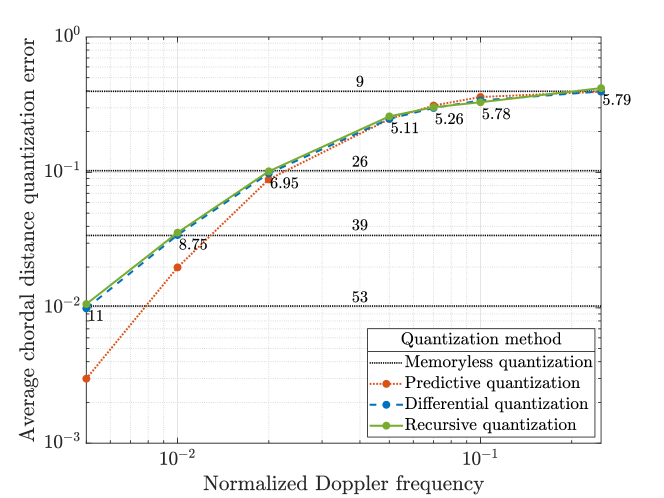
Figure 1: Average quantization distortion on $\mathcal{G}\left(6,2\right)$ versus normalized Doppler frequency. The differential and predictive quantizers provide 6 bits of feedback per time instant; the average number of feedback bits of the recursive multi-stage quantizer is written next to the data points.

In our first simulation, we compare recursive multi-stage quantization to differential and predictive Grassmannian quantization, utilizing the same simulation setup and quantizers as in [22]. Specifically, the channel matrices $\mathbf{H}[k]$ of dimension $n\times m=6\times 2$ are from a Rayleigh fading distribution and are temporally correlated according to Clarke’s Doppler spectrum [27] by employing the sum-of-sinusoids approach of [34]. The predictive and differential quantizers, as proposed in [21], provide 6 bits of feedback per time instant. For comparison, we also show the performance of memoryless single-stage quantization (without selective CSI update) for 9, 26, 39 and 53 bits of feedback, respectively. For the recursive multi-stage quantizer, we have selected the number of quantization bits per stage to achieve the same average performance as the differential quantizer. The average feedback overhead of the recursive quantizer with selective stage update is written next to the simulated data points in Fig. 1.

We observe in Fig. 1 that at low Doppler frequencies the differential and predictive quantizers are more effective in exploiting temporal correlation than the recursive quantizer with selective stage update, as they require only 6 bits of feedback. However, they involve on-the-fly adaptation of the entire quantization codebook at each time instant, which is hard to realize in practice. At moderate to higher Doppler frequencies all three approaches achieve very similar performance. In terms of complexity, though, the recursive quantizer is a lot more tractable, as it does not require any codebook adaptations.

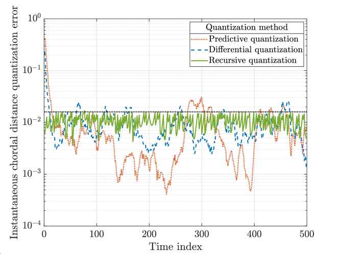
Figure 2: Trace of the quantization error on $\mathcal{G}\left(6,2\right)$ over time for the differential, predictive and recursive quantizers and a normalized Doppler of $\nu_{d}=0.005$.

TABLE II: Classification and average distortion performance of the individual stages of the recursive multi-stage quantizer realized by the neural network structure of section III-C for a codebook size of 6 bits per stage.

Stage	1	3	5	7	9	11	13	15	17	19	21	23	25	27	29	31
Dimension	32$\times$1	30$\times$1	28$\times$1	26$\times$1	24$\times$1	22$\times$1	20$\times$1	18$\times$1	16$\times$1	14$\times$1	12$\times$1	10$\times$1	8$\times$1	6$\times$1	4$\times$1	2$\times$1
Distortion	5.2 e-4	5.6 e-4	5.9 e-4	6.4 e-4	7.0 e-4	7.6 e-4	8.4 e-4	9.4 e-4	1.1 e-3	1.2 e-3	1.4 e-3	1.8 e-3	2.3 e-3	3.2 e-3	5.4 e-3	13.2 e-3
Exhaustive	5.0 e-4	5.4 e-4	5.8 e-4	6.2 e-4	6.8 e-4	7.4 e-4	8.2 e-4	9.2 e-4	1.0 e-3	1.1 e-3	1.3 e-3	1.7 e-3	2.2 e-3	3.1 e-3	5.1 e-3	13.1 e-3

In Fig. 2, we show an exemplary trace of the instantaneous chordal distance quantization error of recursive, differential and predictive quantization for a normalized Doppler frequency of $\nu_{d}=0.005$. We observe that the recursive quantizer, in contrast to the other two, has no convergence phase and exhibits relatively predictable quantization performance, which is basically dictated by the hysteresis parameters of the selective stage update. In this example, we have selected $c_{u}=2$ and $c_{\ell}=1.5$. The black-dotted line in the figure corresponds to the maximally acceptable distortion $c_{u}\,\mathrm{\bar{d}_{c}^{2}}$, which determines when a stage update takes place. For predictive and differential quantization, the performance shows larger variations over time, with increasing distortion whenever the quantizer cannot keep up with the temporal subspace variation of the channel.

In our second simulation, we consider quantization on $\mathcal{G}\left(32,1\right)$ and employ a Gauss-Markov channel model to generate the temporally correlated channel vectors according to $\mathbf{h}[k]=\alpha\mathbf{h}[k-1]+\sqrt{1-\alpha^{2}}\mathbf{g}[k]$, with i.i.d. $\mathbf{g}[k]\sim\mathcal{CN}\left(\bm{0},\mathbf{I}_{n}\right)$ and $\alpha=J_{0}\left(2\pi\nu_{d}\right)$. We select the codebook sizes to achieve an average chordal distance quantization distortion of $\mathrm{\bar{d}_{c}^{2}}=0.06$. For single-stage quantization this requires a codebook size of 125 bits. Obviously, we cannot implement a codebook that is this large; the results of single-stage quantization are therefore based on the theoretic performance investigations of RVQ provided in [32]. For recursive quantization, we employ 31 stages and use a codebook size of 6 bits per stage, i.e., a total feedback overhead of 186 bits when all stages are updated. The individual stages of the recursive quantizer are realized by the classification neural network explained in Section III-C. We summarize the normalized chordal distance distortion of the network in Table II. The classification accuracy of the individual stages of the quantizer lies at approximately 90%; however, the incurred average chordal distance distortion penalty compared to an exhaustive search is negligible.

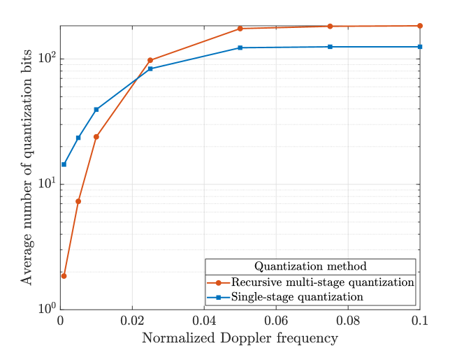
Figure 3: Average number of quantization bits on $\mathcal{G}\left(32,1\right)$ versus normalized Doppler frequency for recursive multi-stage and single-stage quantization.

In Fig. 3, we show the average number of quantization bits of single- and multi-stage quantization with selective CSI/stage update to achieve an average distortion of $\mathrm{\bar{d}_{c}^{2}}=0.06$ as a function of the normalized Doppler frequency. We observe that at low Doppler frequencies the recursive multi-stage quantizer requires less feedback overhead than the single-stage quantizer, as it can selectively update just a subset of the stages of the quantizer. This behavior is investigated in more detail in Fig. 4, where we plot the relative frequency of the number of updated stages of the quantizer. We can see that for small Doppler frequencies in most cases no or just few of the later stages of the quantizer are updated, whereas for high Doppler frequencies almost all stages have to be updated every time.

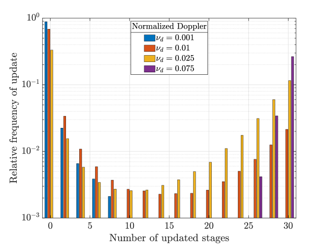
Figure 4: Relative frequency of the number of updated stages of the recursive multi-stage quantizer for different normalized Doppler frequencies.

V Conclusion

In this paper, we have extended recursive Grassmannian multi-stage quantization to exploit temporal channel correlations by selectively updating the individual stages of the quantizer, depending on the achieved distortion. We have shown that this approach performs similar to differential/predictive Grassmannian quantization at moderate to high Doppler frequencies, yet without requiring complicated quantization codebook adaptations. We have furthermore shown that multi-stage quantization can effectively be combined with neural network structures, as the number of classes per stage is sufficiently small to enable accurate DNN classification.

References

- [1] D. Love, R. Heath, Jr., V. Lau, D. Gesbert, B. Rao, and M. Andrews, “An overview of limited feedback in wireless communication systems,” IEEE Journal on Selected Areas in Communications, vol. 26, no. 8, Oct. 2008.
- [2] J. Choi, Z. Chance, D. Love, and U. Madhow, “Noncoherent trellis coded quantization: A practical limited feedback technique for massive MIMO systems,” IEEE Transactions on Communications, vol. 61, no. 12, pp. 5016–5029, December 2013.
- [3] J. Park and R. W. Heath, “Multiple-antenna transmission with limited feedback in device-to-device networks,” IEEE Wireless Communications Letters, vol. 5, no. 2, pp. 200–203, 2016.
- [4] G. Kwon and H. Park, “Limited feedback hybrid beamforming for multi-mode transmission in wideband millimeter wave channel,” IEEE Transactions on Wireless Communications, vol. 19, no. 6, pp. 4008–4022, 2020.
- [5] A. Medra and T. N. Davidson, “Incremental Grassmannian feedback schemes for multi-user MIMO systems,” IEEE Transactions on Signal Processing, vol. 63, no. 5, pp. 1130–1143, 2015.
- [6] A. Decurninge and M. Guillaud, “Cube-split: Structured quantizers on the grassmannian of lines,” in IEEE Wireless Communications and Networking Conference, pp. 1–6, March 2017.
- [7] V. V. Ratnam, A. F. Molisch, O. Y. Bursalioglu, and H. C. Papadopoulos, “Hybrid beamforming with selection for multiuser massive MIMO systems,” IEEE Transactions on Signal Processing, vol. 66, no. 15, pp. 4105–4120, 2018.
- [8] S. Schwarz, M. Rupp, and S. Wesemann, “Grassmannian product codebooks for limited feedback massive MIMO with two-tier precoding,” IEEE Journal of Selected Topics in Signal Processing, vol. 13, no. 5, pp. 1119–1135, Sep. 2019.
- [9] I. S. Dhillon, R. Heath, Jr., T. Strohmer, and J. A. Tropp, “Constructing packings in Grassmannian manifolds via alternating projection,” ArXiv e-prints, Sept. 2007.
- [10] H. E. A. Laue and W. P. du Plessis, “A coherence-based algorithm for optimizing rank-1 Grassmannian codebooks,” IEEE Signal Processing Letters, vol. 24, no. 6, pp. 823–827, 2017.
- [11] B. Tahir, S. Schwarz, and M. Rupp, “Constructing Grassmannian frames by an iterative collision-based packing,” IEEE Signal Processing Letters, vol. 26, no. 7, pp. 1056–1060, July 2019.
- [12] X. Luo, P. Cai, X. Zhang, D. Hu, and C. Shen, “A scalable framework for CSI feedback in FDD massive MIMO via DL path aligning,” IEEE Trans. on Signal Processing, vol. 65, no. 18, pp. 4702–4716, Sep. 2017.
- [13] H. Xie, F. Gao, S. Zhang, and S. Jin, “A unified transmission strategy for TDD/FDD massive MIMO systems with spatial basis expansion model,” IEEE Transactions on Vehicular Technology, vol. 66, no. 4, pp. 3170–3184, April 2017.
- [14] S. Schwarz, “Robust full-dimension MIMO transmission based on limited feedback angular-domain CSIT,” EURASIP Journal on Wireless Communications and Networking, vol. 2018, no. 1, pp. 1–20, Mar 2018.
- [15] T. Wang, C. Wen, S. Jin, and G. Y. Li, “Deep learning-based CSI feedback approach for time-varying massive MIMO channels,” IEEE Wireless Communications Letters, vol. 8, no. 2, pp. 416–419, April 2019.
- [16] Z. Liu, L. Zhang, and Z. Ding, “Exploiting bi-directional channel reciprocity in deep learning for low rate massive MIMO CSI feedback,” IEEE Wireless Communications Letters, vol. 8, no. 3, pp. 889–892, 2019.
- [17] J. Jang, H. Lee, S. Hwang, H. Ren, and I. Lee, “Deep learning-based limited feedback designs for MIMO systems,” IEEE Wireless Communications Letters, vol. 9, no. 4, pp. 558–561, 2020.
- [18] T. Inoue and R. Heath, Jr., “Grassmannian predictive coding for delayed limited feedback MIMO systems,” in 47th Annual Allerton Conference on Communication, Control, and Computing, Oct. 2009.
- [19] D. Sacristan-Murga and A. Pascual-Iserte, “Differential feedback of MIMO channel Gram matrices based on geodesic curves,” IEEE Trans. on Wireless Communications, vol. 9, no. 12, pp. 3714–3727, Dec. 2010.
- [20] O. El Ayach and R. Heath, Jr., “Grassmannian differential limited feedback for interference alignment,” IEEE Transactions on Signal Processing, vol. 60, no. 12, pp. 6481–6494, Dec 2012.
- [21] S. Schwarz, R. Heath, Jr., and M. Rupp, “Adaptive quantization on the Grassmann-manifold for limited feedback multi-user MIMO systems,” in 38th International Conference on Acoustics, Speech and Signal Processing, pp. 5021 – 5025, Vancouver, Canada, May 2013.
- [22] S. Schwarz and M. Rupp, “Predictive quantization on the Stiefel manifold,” IEEE Signal Processing Letters, vol. 22, no. 2, pp. 234–238, 2015.
- [23] Y. Ge, Z. Zeng, T. Zhang, and Y. Liu, “Spatio-temporal correlated channel feedback for massive MIMO systems,” in IEEE/CIC International Conference on Communications in China, pp. 1–5, 2018.
- [24] C. Lu, W. Xu, H. Shen, J. Zhu, and K. Wang, “Mimo channel information feedback using deep recurrent network,” IEEE Communications Letters, vol. 23, no. 1, pp. 188–191, 2019.
- [25] X. Li and H. Wu, “Spatio-temporal representation with deep neural recurrent network in mimo csi feedback,” IEEE Wireless Communications Letters, vol. 9, no. 5, pp. 653–657, 2020.
- [26] S. Schwarz and M. Rupp, “Reduced complexity recursive grassmannian quantization,” IEEE Signal Processing Letters, vol. 27, pp. 321–325, 2020.
- [27] R. H. Clarke, “A statistical theory of mobile radio reception,” Bell Systems Technical Journal, vol. 47, pp. 957–1000, 1968.
- [28] N. Jindal, “MIMO broadcast channels with finite-rate feedback,” IEEE Transactions on Information Theory, vol. 52, no. 11, p. 5, Nov. 2006.
- [29] N. Ravindran and N. Jindal, “Limited feedback-based block diagonalization for the MIMO broadcast channel,” IEEE Journal on Selected Areas in Communications, vol. 26, no. 8, pp. 1473 –1482, Oct. 2008.
- [30] M. Rezaee and M. Guillaud, “Limited feedback for interference alignment in the K-user MIMO interference channel,” in Proc. Information Theory Workshop, pp. 1–5, Lausanne, Suisse, September 2012.
- [31] R. Krishnamachari and M. Varanasi, “Interference alignment under limited feedback for MIMO interference channels,” IEEE Transactions on Signal Processing, vol. 61, no. 15, pp. 3908–3917, Aug 2013.
- [32] W. Dai, Y. Liu, and B. Rider, “Quantization bounds on Grassmann manifolds and applications to MIMO communications,” IEEE Trans. on Information Theory, vol. 54, no. 3, pp. 1108 –1123, March 2008.
- [33] S. Schwarz and M. Rupp, “Subspace quantization based combining for limited feedback block-diagonalization,” IEEE Transactions on Wireless Communications, vol. 12, no. 11, pp. 5868–5879, 2013.
- [34] Y. R. Zheng and C. Xiao, “Simulation models with correct statistical properties for Rayleigh fading channels,” IEEE Transactions on Communications, vol. 51, no. 6, pp. 920 – 928, June 2003.