Resummed predictions for hadronic Higgs boson decays

Abstract

We present the NNLL^′ resummed $2$-jettiness distribution for decays of the Standard Model Higgs boson to a $b\bar{b}$-quark pair and to gluons. The calculation exploits a factorisation formula derived using Soft-Collinear Effective Theory, in which large logarithms of the $2$-jettiness are resummed by renormalisation group evolution of the hard, soft and jet contributions to the differential decay rate. We match the resummed predictions to the fixed-order NNLO result using the Geneva framework, extending the validity of the results to all values of the resolution variable and providing a fully exclusive NNLO event generator matched to the Pythia8 parton shower.

1 Introduction

The lack of any definitive signal of New Physics at the Large Hadron Collider (LHC) suggests that the high-energy physics community must be open to alternative ways to probe Beyond the Standard Model (BSM) effects at collider experiments. In particular, precision measurements of the Standard Model (SM) Higgs sector may be a way to indirectly constrain BSM theories which live at scales beyond our reach, both at the LHC and at future lepton colliders or ‘Higgs factories’. It is therefore crucial that theoretical predictions for processes involving the production or decay of the Higgs boson have a precision which matches that of experiment.

In this work we consider the hadronic decays of a Higgs boson to a $b\bar{b}$-quark pair and to gluons. Although these modes are difficult to observe at a hadron collider due to the large QCD background, they may well prove to be useful probes of Higgs physics at a future lepton collider since they contribute significantly to the total width of the Higgs boson.

The dominant decay mode of the Higgs boson is to a $b\bar{b}$-quark pair, with a branching ratio of about 58% deFlorian:2016spz . An accurate measurement of this channel would allow an extraction of the Yukawa coupling $y_{b}$, which is an important input to Higgs studies. The hadronic environment at the LHC makes this a challenging prospect – nevertheless, the decay has been observed recently by both ATLAS and CMS in the $VH$, or Higgsstrahlung, production channel Sirunyan:2018kst ; Aaboud:2018zhk . QCD corrections to the partial width are known up to N⁴LO Baikov:2005rw ; Gorishnii:1983cu ; Gorishnii:1990zu ; Gorishnii:1991zr ; Becchi:1980vz ; Sakai:1980fa ; Chetyrkin:1996sr ; Chetyrkin:1997vj , and fully differential NNLO calculations have also been available for quite some time Anastasiou:2011qx ; DelDuca:2015zqa . Recently, the fully differential N³LO calculation has also been completed Mondini:2019gid .

The decay channel to gluons, on the other hand, proceeds via a top-quark loop and contributes around 8% to the total width. Since QCD corrections to this channel are indistinguishable from the $b\bar{b}$-quark case at higher orders in perturbation theory, one should consider the classes of processes together to obtain a total hadronic width, as performed in Ref. Davies:2017xsp . Nevertheless, at NNLO and in the case of kinematically massless $b$-quarks the processes can be fully separated, since interference terms between the diagrams vanish. Related complications which arise at N³LO have been studied in Ref. Mondini:2020uyy . In the case of massive $b$-quarks, these interference terms can no longer be neglected – their impact has been studied in Ref. Primo:2018zby and a full NNLO calculation in the massive case has been carried out in Refs. Bernreuther:2018ynm ; Behring:2020uzq .

In the limit that $M_{H}\ll 2m_{t}$, the top-quark loop which couples the Higgs boson to gluons can be integrated out to obtain an effective theory with five light active flavours in which the interaction is local. This simplifies the inclusion of QCD corrections and has allowed calculations to be performed at NNLO Chetyrkin:1997iv ; Caola:2019pfz and, for the total width, at N³LO Baikov:2006ch and N⁴LO Herzog:2017dtz . The effect of including a finite top-quark mass on the total width has also been studied in Ref. Schreck:2007um .

In light of the importance of Higgs physics, several other predictions at various accuracies and using different approximations are available beyond those listed here. A complete review of the state of the theoretical calculations for Higgs boson production and decay processes, including the calculation of electroweak corrections, can be found in Ref. Spira:2016ztx .

In a recent publication Gao:2019mlt , the distributions of the thrust variable in these decay processes were considered and fixed-order computations up to approximate NNLO (which contribute at $\mathcal{O}(\alpha_{\rm s}^{3})$ relative to a Born $H\rightarrow b\bar{b}/gg$ process) were performed. In that work, the authors noted the poor convergence of the perturbative series for both processes and were able to show that the approximate NNLO corrections obtained from the singular terms of a SCET-derived factorisation formula could ameliorate the scale dependence of the calculations. They also acknowledged several shortcomings of their calculation, one of which related to the size of the logarithms $\log^{n}\tau/\tau$ which are not resummed in a purely fixed-order computation and spoil predictivity in the small $\tau$ region. Here, we provide resummed predictions at NNLL^′ accuracy which complement the results of Ref. Gao:2019mlt . Compared to NNLL, the resummation at NNLL^′ accuracy incorporates the complete $\mathcal{O}(\alpha_{\rm s}^{2})$ singular structure for $\mathcal{T}_{2}\to 0$, i.e. all 2-loop virtual and corresponding real corrections, allowing us to consistently match to NNLO.

Using the Geneva formalism developed in Refs. Alioli:2012fc ; Alioli:2013hqa ; Alioli:2015toa , we are also able to construct IR-finite events which combine the advantages of the resummed and fixed-order calculations and are matched to a parton shower.

Having a Geneva implementation of the $H\rightarrow b\bar{b}$ process will also allow us to produce an NNLOPS generator for the signal process $pp\rightarrow V(H\to b\bar{b})$. This can be achieved by combining the Higgs boson decay presented here with our previous calculation of the $VH$ production process Alioli:2019qzz in the narrow width approximation. Fixed-order calculations for the full $pp\rightarrow Vb\bar{b}$ process were performed in Ref. Ferrera:2017zex ; Caola:2017xuq ; Gauld:2019yng in the massless approximation – more recently, a calculation with massive $b$-quarks also appeared Behring:2020uzq . An NNLOPS generator for $W(H\to b\bar{b})$ production via the MiNLO method Hamilton:2012rf ; Hamilton:2013fea ; Monni:2019whf ; Monni:2020nks was presented in Astill:2018ivh , while a separate NNLOPS $H\rightarrow b\bar{b}$ generator was also made available in Ref. Bizon:2019tfo . Nonetheless, we believe an independent implementation of the combined corrections to both production and decay in the Geneva framework will provide a useful cross-check of previous results. We leave this development to a future publication.

This paper is organised as follows. In sec. 2, we briefly explain how resummed predictions are obtained from a factorisation formula derived in soft-collinear effective theory and provide numerical results for the resummed $\mathcal{T}_{2}$ distribution in $H\rightarrow b\bar{b}$ and $H\rightarrow gg$. In sec. 3, we briefly recap the main features of the Geneva method relevant for the processes at hand. In particular, we discuss various implementation details, as well as how the matching to the parton shower is achieved. We present our Geneva results in sec. 4. Finally, we report our conclusions and directions for future work in sec. 5, while we detail the construction of the phase space mappings used and the analytical NNLO decay rates in Apps. A and B respectively.

2 Resummation from Soft-Collinear Effective Theory

In this section we present, for the first time, the NNLL^′ resummation of the $2$-jettiness observable, $\mathcal{T}_{2}$, for the decay of a Higgs boson into a pair of $b$-quarks. We also provide results at the same accuracy for the Higgs boson decay into gluons, which were first presented in Ref. Mo:2017gzp . We present numerical results for the dimensionless $\tau\equiv\mathcal{T}_{2}/(2\,M_{H})$ distribution, where $M_{H}$ is the mass of the Higgs boson.

2.1 Formulation

Our basic resolution parameter for the hadronic decays of the Higgs boson is the $2$-jettiness, defined as

$$\mathcal{T}_{2}=2\min_{\vec{n}}\sum_{k}\left(E_{k}-\lvert\vec{n}\cdot\vec{p_{k}}\rvert\right)\,,$$ (1)

where $k$ runs over all final state particles with momenta $p_{k}=(E_{k},\vec{p}_{k})$ and $\vec{n}$ is the unit $3$-vector resulting from the minimisation procedure. In the case where all final-state particles are massless, it is related to the more familiar thrust $T$, which was widely studied for $e^{+}e^{-}$ collisions Catani:1991kz ; Catani:1992ua and extended to hadronic collisions in Ref. Banfi:2004nk , by the relation $\mathcal{T}_{2}=2E_{\mathrm{cm}}(1-T)$. For the decays that we consider, we work in the rest frame of the Higgs boson and always have that $E_{\mathrm{cm}}=M_{H}$. Exactly like the thrust variable, the $2$-jettiness is constrained kinematically $(0\leq\mathcal{T}_{2}\leq M_{H})$ and its value is related to the spatial distribution of the radiation: in the limit $\mathcal{T}_{2}\rightarrow 0$ the final state consists of two pencil-like jets, while for $\mathcal{T}_{2}\sim M_{H}$ there are three or more jets distributed in a more spherical configuration.

We consider the decay rate differential in $\mathcal{T}_{2}$ of a Higgs boson to either a $b\bar{b}$-quark pair or to a pair of gluons. We consider massless $b$-quarks with a finite Yukawa coupling to the Higgs $y_{b}$. In the gluon case, we work in an effective theory in which the top-quark loop that couples the Higgs boson to gluons has been integrated out, leaving an effective local operator $Hgg$.

The Born level decay rates for the two processes considered are given by

$$\Gamma_{\mathrm{B}}^{b}(\mu)=\frac{y_{b}^{2}(\mu)\,N_{c}\,M_{H}}{8\pi},\qquad\Gamma_{\mathrm{B}}^{g}(\mu)=\frac{\alpha_{\rm s}^{2}(\mu)\,G_{F}\,M_{H}^{3}}{36\pi^{3}\,\sqrt{2}}\,.$$ (2)

It has been shown, both in QCD and SCET, that the differential decay rate factorises in the small $\mathcal{T}_{2}$ limit Korchemsky:1999kt ; Catani:1992ua ; Fleming:2007qr ; Schwartz:2007ib as

$$\frac{\mathrm{d}\Gamma^{i}}{\mathrm{d}\mathcal{T}_{2}}=\Gamma_{\mathrm{B}}^{i}(\mu)\ H^{i}(M_{H},\mu)\int\mathrm{d}p_{n}^{2}\mathrm{d}p_{\bar{n}}^{2}\mathrm{d}k\,\delta\left(\mathcal{T}_{2}-\frac{2(p_{n}^{2}+p_{\bar{n}}^{2})}{M_{H}}-k\right)J_{n}^{i}(p_{n}^{2},\mu)J_{\bar{n}}^{i}(p_{\bar{n}}^{2},\mu)S^{i}(k,\mu)\,$$ (3)

where the index $i=b,g$ indicates the process in question.

The decay rate has been factorised into a hard contribution $H^{i}(M_{H},\mu)$, a soft function $S^{i}(k,\mu)$ and two jet functions $J_{n}^{i}(p_{n}^{2},\mu)$ and $J_{\bar{n}}^{i}(p_{\bar{n}}^{2},\mu)$. The hard function is defined as the square of the Wilson coefficients which match the full theory (the SM) onto SCET. In the gluon case, an additional matching is required from the heavy-top limit effective theory we are working in onto the SM – thus, the hard functions can be written as

$$H^{b}(M_{H},\mu) =|C^{b}_{\mathrm{SCET}}(M_{H},\mu)|^{2}$$

$$H^{g}(M_{H},\mu) =|C^{g}_{\mathrm{SCET}}(M_{H},\mu)|^{2}\,|C_{t}(m_{t},\mu)|^{2}\,.$$ (4)

The jet functions describe collinear radiation from the Born-level partons along the jet directions $n$ and $\bar{n}$, which can be chosen without loss of generality to be orientated along $\hat{z}$, viz. $n=(1,0,0,1)$ and $\bar{n}=(1,0,0,-1)$. The soft function accounts for all soft radiation.

Each component in the factorisation theorem must be evaluated at its own characteristic scale in order to prevent the appearance of large logarithms, viz. $\mu_{H}\sim M_{H}$, $\mu_{J}\sim\sqrt{\phantom{\big{(}}\!\!\!\mathcal{T}_{2}M_{H}}$, $\mu_{S}\sim\mathcal{T}_{2}$. However, since the decay rate must be evaluated at a single scale, we evolve the separate functions to a common scale $\mu$ via renormalisation group (RG) evolution and in so doing resum the large logarithms of ratios of scales which appear.

The resummed spectrum, differential in the Born kinematics, can then be written as

$$\frac{\mathrm{d}\Gamma^{i,\rm resum}}{\mathrm{d}\Phi_{2}\mathrm{d}\mathcal{T}_{2}} =\frac{\mathrm{d}\Gamma_{\mathrm{B}}^{i}(\mu)}{\mathrm{d}\Phi_{2}}H^{i}(M_{H},\mu_{H})\,U^{i}_{H}(\mu_{H},\mu)\otimes\bigl{[}S^{i}(\mu_{S})\otimes U^{i}_{S}(\mu_{S},\mu)\bigr{]}$$

$$\qquad\otimes\bigl{[}J^{i}_{n}(\mu_{J})\otimes U^{i}_{J}(\mu_{J},\mu)\bigr{]}\otimes\bigl{[}J^{i}_{\bar{n}}(\mu_{J})\otimes U^{i}_{J}(\mu_{J},\mu)\bigr{]}\,$$ (5)

where $\mathrm{d}\Gamma_{\mathrm{B}}^{i}(\mu)/\mathrm{d}\Phi_{2}$ indicates the Born decay rate differential in the two-body phase space and we have used $\otimes$ to denote the convolutions, dropping the explicit dependence on the convolution variables. The ingredients necessary for NNLL^′ accuracy are all available in the literature and many have been compiled in Ref. Gao:2019mlt . For the $H\rightarrow b\bar{b}$ case, we take the hard function from Ref. Gao:2019mlt . Since we are considering only massless $b$-quarks, we can use the soft and jet functions as implemented in Ref. Alioli:2012fc (and first calculated at NNLO in Refs. Kelley:2011ng ; Monni:2011gb ; Becher:2006qw ) for $e^{+}e^{-}\to jj$, also recycling the evolution kernels from that work. For the $H\rightarrow gg$ case, the fully expanded hard function, including contributions to the $Hgg$ effective vertex from both SCET and the effective theory where the top-quark is integrated out, appears in Ref. Mo:2017gzp . The NNLO jet function Becher:2010pd and the evolution kernels are also given therein, while we obtain the soft function via a Casimir rescaling of the $H\to b\bar{b}$ case.

2.2 Numerical results

We have implemented the resummed calculation, eq. (2.1), in the Geneva framework (see sec. 3) up to NNLL^′ order, for which we now present results. Throughout the calculation we choose a Higgs boson mass $M_{H}=125.09~{}\,\mathrm{GeV}$ and set $\alpha_{\rm s}(M_{Z})=0.118$, $G_{F}=1.16639\times 10^{-5}$. We set the renormalisation scale to be $\mu_{R}=M_{H}$ and run the $b$-quark Yukawa $y_{b}$ at two-loop order, setting $m_{b}=4.92\,\mathrm{GeV}$.

The normalised distributions in $\tau\equiv\mathcal{T}_{2}/(2M_{H})$ are shown in fig. 1 for both the $H\to b\bar{b}$ and the $H\to gg$ decay channels.

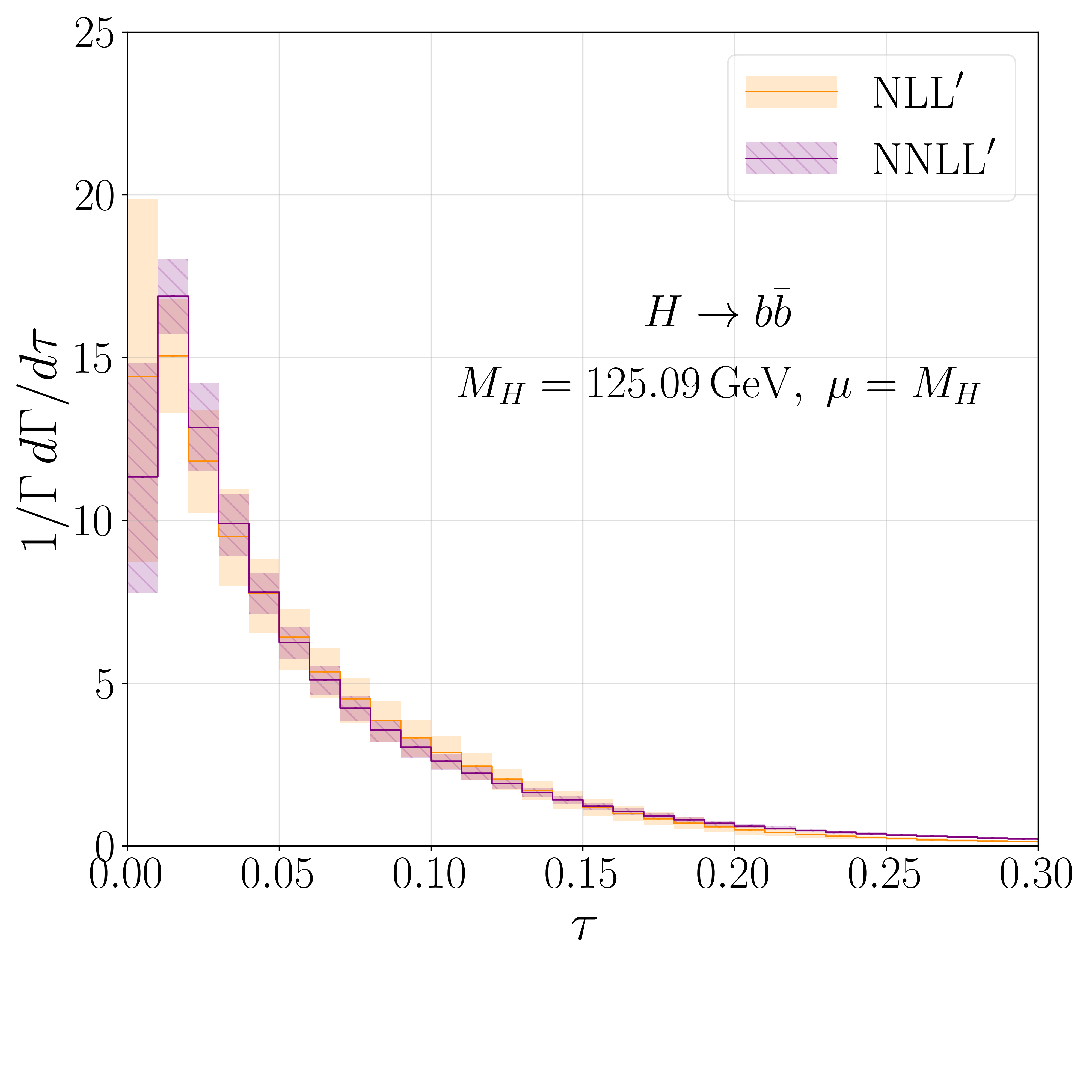
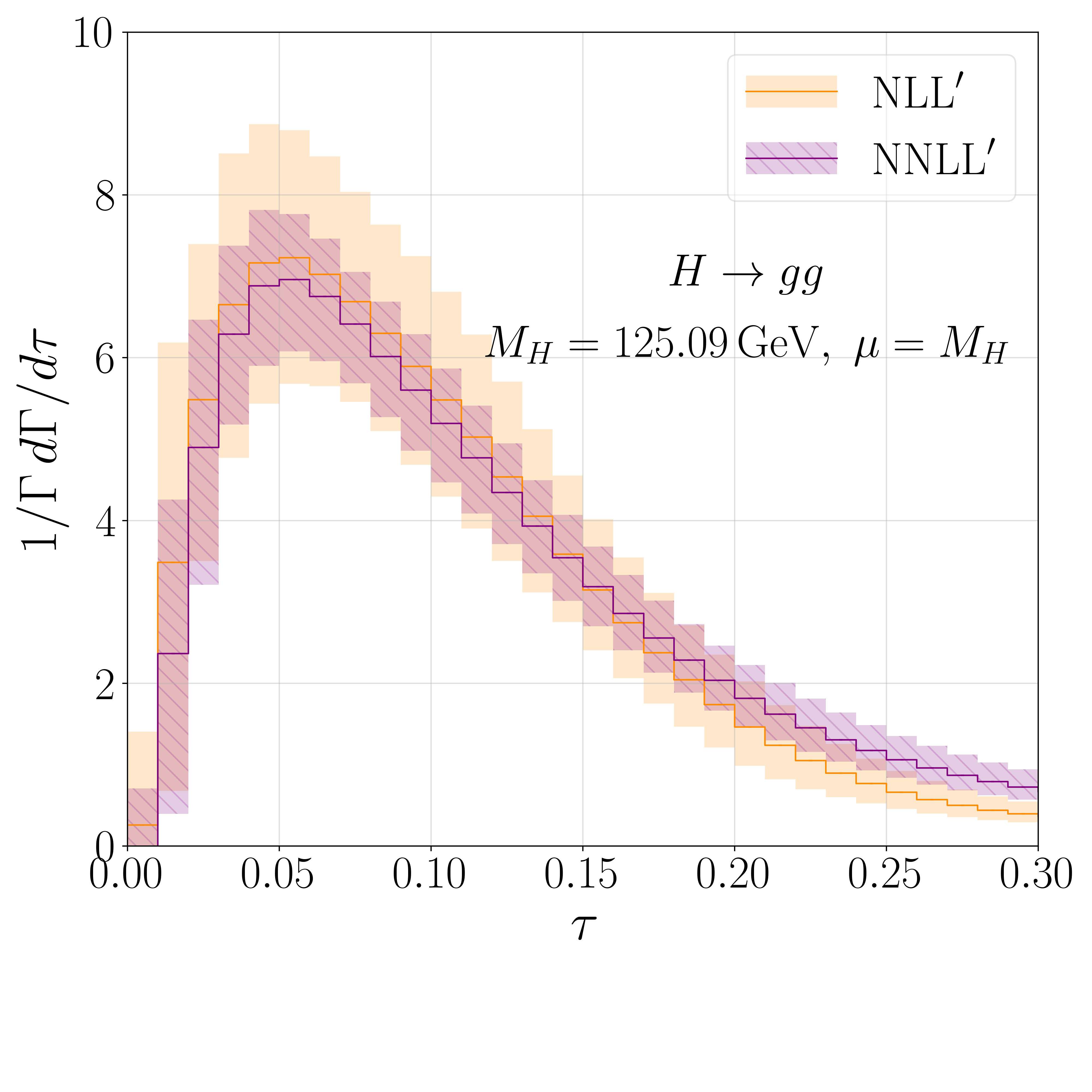
Figure 1: The normalised, resummed spectrum in $\tau\equiv\mathcal{T}_{2}/(2M_{H})$, corresponding to eq. (2.1), at NLL^′ and NNLL^′. The left panel shows the process $H\rightarrow b\bar{b}$, the right shows $H\rightarrow gg$.

These predictions have been obtained with the scale choices detailed in sec. 3.2.1 and the uncertainties calculated as explained there.

Because of the resummation of large logarithms of $\tau$, our results provide a physical description at small $\tau$, as can be seen in fig. 1, improving on the resummed-expanded results presented in Ref. Gao:2019mlt . However, the range of validity of the resummed calculation is still limited to low $\tau$ values, since the factorisation formula we rely on (eq. (3)) is only valid there. Comparing the two decay channels, we see that the $H\to b\bar{b}$ process presents a higher peak, located at a lower value of $\tau$, with a narrower width. The peak of the $\tau$ distribution in the $H\to gg$ case is instead lower and shifted to larger values of $\tau$, with a broader width. This behaviour is in line with expectations based on a naive analysis of the Casimir scaling of the two processes.

In order to extend the validity of the calculation to all values of $\tau$, one needs to match the resummed result to the fixed-order calculation, which provides the physical behaviour at large $\tau$. Indeed, in this region, the nonsingular contribution becomes sizeable and exponentiating the singular contribution is no longer the correct approach. The matching of fixed-order calculations to resummation has long been established at the level of the resummed observable: the most straightforward approach simply adds the results for the resummed and fixed-order distributions in the $\tau$ variable and then subtracts the expansion of the resummed result up to the same order included in the fixed-order result. In this way the calculation is free from doubly counted contributions up to the given perturbative order and includes all the higher-order terms properly resummed.

While the approach just outlined works flawlessly for the $\tau$ distribution we are resumming, it is not directly applicable to the construction of a fully exclusive event generator. In the next section, sec. 3, we show how this can be achieved by means of the Geneva method, allowing us to perform the matching at the fully differential level.

3 Implementation in the Geneva framework

3.1 Geneva in a nutshell

The Geneva framework allows the matching of a resummed to a fixed-order calculation and thence to parton shower programs such as Pythia Sjostrand:2014zea . In so doing, it provides theoretical predictions which are accurate over the whole phase space and which describe realistic events of high multiplicity. These can then be hadronised and fed into the analysis routines used by the experimental collaborations. The method for separating events into different multiplicity bins and for performing the matching has already been described thoroughly in Refs. Alioli:2012fc ; Alioli:2015toa and related references. Therefore, in this context, we limit ourselves to restating the primary outcomes as applicable to the case of Higgs boson hadronic decays up to NNLL${}^{\prime}_{\mathcal{T}}$+NNLO₂ accuracy. We remind the reader that in order to achieve a sensible separation between the exclusive $3$-jet and the inclusive $4$-jet decay rates, we must also perform the resummation of $\mathcal{T}_{3}^{\mathrm{cut}}$ at least at leading-log order, as we do in the following.

Dropping the process label $i$ for ease of notation, the Geneva Monte Carlo expressions for the exclusive $2$-jet, $3$-jet and the inclusive $4$-jet rates are given by

$$\frac{\mathrm{d}\Gamma^{\textsc{mc}}_{2}}{\mathrm{d}\Phi_{2}}(\mathcal{T}_{2}^{\mathrm{cut}}) =\frac{\mathrm{d}\Gamma^{\rm NNLL^{\prime}}}{\mathrm{d}\Phi_{2}}(\mathcal{T}_{2}^{\mathrm{cut}})-\biggl{[}\frac{\mathrm{d}\Gamma^{\rm NNLL^{\prime}}}{\mathrm{d}\Phi_{2}}(\mathcal{T}_{2}^{\mathrm{cut}})\biggr{]}_{\rm NNLO_{2}}+(B_{2}+V_{2}+W_{2})(\Phi_{2})$$

$$\quad+\int\!\frac{\mathrm{d}\Phi_{3}}{\mathrm{d}\Phi_{2}}\,(B_{3}+V_{3})(\Phi_{3})\,\theta[\mathcal{T}_{2}(\Phi_{3})<\mathcal{T}_{2}^{\mathrm{cut}}]$$

$$\quad+\int\!\frac{\mathrm{d}\Phi_{4}}{\mathrm{d}\Phi_{2}}\,B_{4}(\Phi_{4})\,\theta[\mathcal{T}_{2}(\Phi_{4})<\mathcal{T}_{2}^{\mathrm{cut}}]\,,$$ (6)

$$\frac{\mathrm{d}\Gamma^{\textsc{mc}}_{3}}{\mathrm{d}\Phi_{3}}(\mathcal{T}_{2}>\mathcal{T}_{2}^{\mathrm{cut}};\mathcal{T}_{3}^{\mathrm{cut}}) =\Bigg{\{}\frac{\mathrm{d}\Gamma^{\rm NNLL^{\prime}}}{\mathrm{d}\Phi_{2}\mathrm{d}\mathcal{T}_{2}}\mathcal{P}(\Phi_{3})+(B_{3}+V_{3}^{C})(\Phi_{3})-\biggl{[}\frac{\mathrm{d}\Gamma^{\rm NNLL^{\prime}}}{\mathrm{d}\Phi_{2}\mathrm{d}\mathcal{T}_{2}}\mathcal{P}(\Phi_{3})\,\biggr{]}_{\mathrm{NLO}_{3}}\Bigg{\}}$$

$$\quad\times U_{3}(\Phi_{3},\mathcal{T}_{3}^{\mathrm{cut}})\,\theta(\mathcal{T}_{2}>\mathcal{T}_{2}^{\mathrm{cut}})$$

$$\quad+\int\!\biggl{[}\frac{\mathrm{d}\Phi_{4}}{\mathrm{d}\Phi_{3}^{\mathcal{T}}}\,B_{4}(\Phi_{4})\,\theta[\mathcal{T}_{2}(\Phi_{4})>\mathcal{T}_{2}^{\mathrm{cut}}]\,\theta(\mathcal{T}_{3}<\mathcal{T}_{3}^{\mathrm{cut}})$$

$$\quad\quad\quad\quad-\frac{\mathrm{d}\Phi_{4}}{\mathrm{d}\Phi_{3}^{C}}\,C_{4}(\Phi_{4})\,\theta(\mathcal{T}_{2}>\mathcal{T}_{2}^{\mathrm{cut}})\biggr{]}$$

$$\quad-B_{3}(\Phi_{3})\,U_{3}^{(1)}(\Phi_{3},\mathcal{T}_{3}^{\mathrm{cut}})\,\theta(\mathcal{T}_{2}>\mathcal{T}_{2}^{\mathrm{cut}})\,,$$ (7)

$$\frac{\mathrm{d}\Gamma^{\textsc{mc}}_{3}}{\mathrm{d}\Phi_{3}}(\mathcal{T}_{2}\leq\mathcal{T}_{2}^{\mathrm{cut}}) =\bar{\Theta}^{\mathrm{FKS}}_{\mathrm{map}}(\Phi_{3})\,(B_{3}+V_{3})\,(\Phi_{3})\,\theta(\mathcal{T}_{2}<\mathcal{T}^{\mathrm{cut}}_{2})\,,$$ (8)

$$\frac{\mathrm{d}\Gamma^{\textsc{mc}}_{\geq 4}}{\mathrm{d}\Phi_{4}}(\mathcal{T}_{2}>\mathcal{T}_{2}^{\mathrm{cut}},\mathcal{T}_{3}>\mathcal{T}_{3}^{\mathrm{cut}})=$$

$$\qquad\Bigg{\{}\frac{\mathrm{d}\Gamma^{\rm NNLL^{\prime}}}{\mathrm{d}\Phi_{2}\mathrm{d}\mathcal{T}_{2}}\mathcal{P}(\Phi_{3})+(B_{3}+V_{3}^{C})(\Phi_{3})-\biggl{[}\frac{\mathrm{d}\Gamma^{\rm NNLL^{\prime}}}{\mathrm{d}\Phi_{2}\mathrm{d}\mathcal{T}_{2}}\mathcal{P}(\Phi_{3})\,\biggr{]}_{\mathrm{NLO}_{3}}\Bigg{\}}$$

$$\qquad\times U_{3}^{\prime}(\Phi_{3},\mathcal{T}_{3})\,\theta(\mathcal{T}_{2}>\mathcal{T}_{2}^{\mathrm{cut}})\Big{|}_{\Phi_{3}=\Phi_{3}^{\mathcal{T}}(\Phi_{4})}\!\!\mathcal{P}(\Phi_{4})\,\theta(\mathcal{T}_{3}>\mathcal{T}_{3}^{\mathrm{cut}})$$

$$\qquad+\bigl{\{}B_{4}(\Phi_{4})\,[1-\Theta^{\mathcal{T}}(\Phi_{4})\,\theta(\mathcal{T}_{3}<\mathcal{T}_{3}^{\mathrm{cut}})]$$

$$\qquad-B_{3}(\Phi_{3}^{\mathcal{T}})\,U_{3}^{{(1)}\prime}(\Phi_{3}^{\mathcal{T}},\mathcal{T}_{3})\,\mathcal{P}(\Phi_{4})\,\theta(\mathcal{T}_{3}>\mathcal{T}_{3}^{\mathrm{cut}})\bigr{\}}\,\theta[\mathcal{T}_{2}(\Phi_{4})>\mathcal{T}_{2}^{\mathrm{cut}}]\,,$$ (9)

$$\frac{\mathrm{d}\Gamma^{\textsc{mc}}_{\geq 4}}{\mathrm{d}\Phi_{4}}(\mathcal{T}_{2}>\mathcal{T}_{2}^{\mathrm{cut}},\mathcal{T}_{3}\leq\mathcal{T}_{3}^{\mathrm{cut}})\,=\, B_{4}(\Phi_{4})\,\bar{\Theta}^{\mathcal{T}}(\Phi_{4})\,\theta(\mathcal{T}_{3}<\mathcal{T}_{3}^{\mathrm{cut}})\,\theta\left(\mathcal{T}_{2}(\Phi_{4})>\mathcal{T}_{2}^{\mathrm{cut}}\right)\,,$$ (10)

where the $B_{j}$, $V_{j}$ and $W_{j}$ are the $0$-, $1$- and $2$-loop matrix elements for $j$ partons in the final state.

In the equations above, we have introduced the shorthand notation

$$\frac{\mathrm{d}\Phi_{M}}{\mathrm{d}\Phi_{N}^{\cal O}}=\mathrm{d}\Phi_{M}\,\delta[\Phi_{N}-\Phi^{\cal O}_{N}(\Phi_{M})]\,\Theta^{\cal O}(\Phi_{N})\,,$$ (11)

to indicate that the integration over a region of the $M$-body phase space is done keeping the $N$-body phase space and the value of some specific observable $\cal O$ fixed, with $N\leq M$. The $\Theta^{\cal O}(\Phi_{N})$ term in the previous equation limits the integration to the phase space points included in the singular contribution for the given observable $\cal O$. For example, when generating $3$-body events we use

$$\frac{\mathrm{d}\Phi_{4}}{\mathrm{d}\Phi_{3}^{\mathcal{T}}}\equiv\mathrm{d}\Phi_{4}\,\delta[\Phi_{3}-\Phi^{\mathcal{T}}_{3}(\Phi_{4})]\,\Theta^{\mathcal{T}}(\Phi_{4})\,,$$ (12)

where the map used by the $3\to 4$ splitting has been constructed to preserve $\mathcal{T}_{2}$, i.e.

$$\mathcal{T}_{2}(\Phi_{3}^{\mathcal{T}}(\Phi_{4}))=\mathcal{T}_{2}(\Phi_{4})\,$$ (13)

and $\Theta^{\mathcal{T}}(\Phi_{4})$ defines the projectable region of $\Phi_{4}$ which can be reached starting from a point in $\Phi_{3}$ with a specific value of $\mathcal{T}_{2}$. The usage of a $\mathcal{T}_{2}$-preserving mapping is necessary to ensure that the pointwise singular $\mathcal{T}_{2}$ dependence is alike among all terms in eqs. (3.1) and (3.1) and that the cancellation of said singular terms is guaranteed on an event-by-event basis.

The expressions in eqs. (8) and (10) encode the nonsingular contributions to the $3$- and $4$-jet rates which arise from non-projectable configurations below the corresponding cut. This is highlighted by the appearance of the complementary $\Theta$ functions, $\bar{\Theta}^{\cal O}$, which account for any configuration which is not projectable either because it would result in an invalid underlying-Born flavour structure or because it does not satisfy the $\mathcal{T}_{2}$-preserving mapping (see also Ref. Alioli:2019qzz ).

The term $V_{3}^{C}$ denotes the soft-virtual contribution of a standard NLO local subtraction (in our implementation, we follow the FKS subtraction as detailed in Ref. Frixione:2007vw ). We have that

$$V_{3}^{C}(\Phi_{3})=V_{3}(\Phi_{3})+\int\frac{\mathrm{d}\Phi_{4}}{\mathrm{d}\Phi_{3}^{C}}C_{4}(\Phi_{4})\,,$$ (14)

with $C_{4}$ a singular approximation of $B_{4}$: in practice we use the subtraction counterterms which we integrate over the radiation variables $\mathrm{d}\Phi_{4}/\mathrm{d}\Phi_{3}^{C}$ using the singular limit $C$ of the phase space mapping. $U_{3}$ is a LL Sudakov which resums large logarithms of $\mathcal{T}_{3}$ and $U_{3}^{\prime}$ its derivative with respect to $\mathcal{T}_{3}$. Its exact form is given by

$$U_{3}(\mathcal{T}_{3}^{\mathrm{cut}},\mathcal{T}_{3}^{\mathrm{max}})=\exp\left[-\frac{\alpha_{\rm s}}{2\pi}C_{k}\log^{2}\left(\frac{\mathcal{T}_{3}^{\mathrm{max}}}{\mathcal{T}_{3}^{\mathrm{cut}}}\right)\right]$$ (15)

where the Casimir factor $C_{k}$ depends on the flavour content of the $3$-jet event,
$C_{q\bar{q}g}=2C_{F}+C_{A}$ or $C_{ggg}=3C_{A}$, and we run the coupling at NNLL order.

The term $\mathcal{P}(\Phi_{N+1})$ represents a normalised splitting probability which serves to extend the differential dependence of the resummed terms from the $N$-jet to the $(N\!+\!1)$-jet phase space. For example, in eq. (3.1), the term $\mathcal{P}(\Phi_{3})$ makes the resummed spectrum in the first term (which is naturally differential in the $\Phi_{2}$ variables and $\mathcal{T}_{2}$) differential also in the additional two variables needed to cover the full $\Phi_{3}$ phase space. These splitting probabilities are normalised, i.e. they satisfy

$$\int\!\frac{\mathrm{d}\Phi_{N+1}}{\mathrm{d}\Phi_{N}\mathrm{d}\mathcal{T}_{N}}\,\mathcal{P}(\Phi_{N+1})=1\,.$$ (16)

The two extra variables are chosen to be an energy ratio $z$ and an azimuthal angle $\phi$. In the soft and collinear limit, $z=E_{\mathrm{sister}}/(E_{\mathrm{sister}}+E_{\mathrm{daughter}})$ where the daughter and the sister are assigned to be the pair of particles that are closest according to the $N$-jettiness metric and which therefore set the value of $\mathcal{T}_{N}$, i.e. which minimise the quantity

$$\rho_{ij}=|\vec{p}_{i}|+|\vec{p}_{j}|-|\vec{p}_{i}+\vec{p}_{j}|.$$ (17)

The daughter particle is defined to be the gluon for $q\rightarrow qg$ splittings, the quark for $g\rightarrow q\bar{q}$ and the softer gluon for $g\rightarrow gg$. These definitions in hand, the normalised splitting probability is given by

$$\mathcal{P}(\Phi_{N+1})=\frac{\mathrm{AP}_{\mathrm{sp}}(z,\phi)}{\sum_{\mathrm{sp}}\int^{z_{\mathrm{max}}(\mathcal{T}_{N})}_{z_{\mathrm{min}}(\mathcal{T}_{N})}\mathrm{d}z\mathrm{d}\phi\mathrm{AP}_{\mathrm{sp}}(z,\phi)}\frac{\mathrm{d}\Phi_{N}\mathrm{d}\mathcal{T}_{N}\mathrm{d}z\mathrm{d}\phi}{\mathrm{d}\Phi_{N+1}}\,,$$ (18)

where $\mathrm{AP}_{\mathrm{sp}}(z,\phi)$ is the unregularised Altarelli-Parisi splitting function.

The implementation of the splitting probability requires us to construct the full $\Phi_{N+1}$ phase space from $\Phi_{N}$ and a value of $\mathcal{T}_{N}$. Similarly, we mentioned above that the real integration in the fixed-order part of the calculation requires us to project from $\Phi_{N+1}$ configurations onto $\Phi_{N}$ while preserving the value of $\mathcal{T}_{2}$. Both of these tasks demand a map that satisfies eq. (13) – the construction of such a map is detailed in App. A.

3.2 Implementation details

In this section we discuss the particulars of the implementation of the Higgs boson decay processes in Geneva. Throughout this section we use the same settings and values for SM parameters as in sec. 2.2. In the $H\rightarrow b\bar{b}$ case, we implement the analytic matrix elements found in Ref. DelDuca:2015zqa , while in the $H\rightarrow gg$ case we interface to the OpenLoops package Cascioli:2011va ; Buccioni:2017yxi ; Buccioni:2019sur .

3.2.1 Profile scales

The resummation provided by the RGE of the functions in eq. (3) correctly accounts for logarithms of the form $\log(\mathcal{T}_{2}/2M_{H})$ which become large in size for small values of $\mathcal{T}_{2}$. In the fixed-order region, however, where $\mathcal{T}_{2}$ is larger, such logarithms are more modest in size and continuing to resum them would introduce undesirable higher-order contributions.

We must therefore switch off the resummation before this happens. This can be achieved by setting all scales to a common nonsingular scale in the fixed-order region, $\mu_{\mathrm{NS}}=\mu_{S}=\mu_{J}=\mu_{H}$, which stops the evolution ensuring that the resummed contribution is cancelled out exactly by the resummed-expanded. In order to achieve a smooth transition between the resummation and the fixed-order (FO) regimes, we make use of profile scales $\mu_{J}(\mathcal{T}_{2})$ and $\mu_{S}(\mathcal{T}_{2})$ which interpolate between the characteristic scales and $\mu_{\mathrm{NS}}$ Abbate:2010xh ; Berger:2010xi . Specifically, we have that

$$\mu_{H} =\mu_{\mathrm{NS}}$$

$$\mu_{S}(\mathcal{T}_{2}) =\mu_{\mathrm{NS}}f_{\mathrm{run}}(\mathcal{T}_{2}/2M_{H})$$

$$\mu_{J}(\mathcal{T}_{2}) =\mu_{\mathrm{NS}}\sqrt{f_{\mathrm{run}}(\mathcal{T}_{2}/2M_{H})}\,,$$ (19)

where the common profile function $f_{\mathrm{run}}(x)$ is given by

$$f_{\rm run}(x) =\begin{cases}\vspace{1mm}\displaystyle ax_{0}\left[1+\left(\frac{x}{2x_{0}}\right)^{2}\right]&x\leq 2x_{0}\,,\\ \vspace{1mm}ax&2x_{0}\leq x\leq x_{1}\,,\\ \vspace{1mm}\displaystyle ax+\frac{(2-ax_{2}-ax_{3})(x-x_{1})^{2}}{2(x_{2}-x_{1})(x_{3}-x_{1})}&x_{1}\leq x\leq x_{2}\,,\\ \vspace{1mm}\displaystyle 1-\frac{(2-ax_{1}-ax_{2})(x-x_{3})^{2}}{2(x_{3}-x_{1})(x_{3}-x_{2})}&x_{2}\leq x\leq x_{3}\,,\\ 1&x_{3}\leq x\,.\end{cases}\,.$$ (20)

This form has strict canonical scaling below $x_{1}$ and switches off the resummation above $x_{3}$; for $a=1$ it matches the form of the profiles used in e.g. Ref. Stewart:2013faa .

In order to determine the choice of parameters $a,\,x_{i}$ it is instructive to examine the relative sizes of the singular and nonsingular contributions as a function of $\mathcal{T}_{2}$ to determine where the resummation should be switched off. This is done for the two decay channels as shown in fig. 2. We see that the singular and nonsingular pieces become similar in size at around $\tau\equiv\mathcal{T}_{2}/(2M_{H})\approx 0.3$, and therefore set for both processes

$$\mu_{\mathrm{FO}}\equiv\mu_{\mathrm{NS}} =M_{H}\,, \{x_{1},x_{2},x_{3}\} =\{0.1,0.2,0.3\}\,.$$ (21)

We notice that in the limit $\tau\rightarrow 0$ the singular contribution becomes an increasingly good approximation to the fixed-order result, reflecting the proper cancellation of the singular terms between the fixed-order and resummed-expanded parts of the calculation. We set the remaining parameters $a=1,\,ax_{0}=3\,\,\mathrm{GeV}/M_{H}$ for the $gg$ channel following Ref. Mo:2017gzp , while for the $b\bar{b}$ channel we set $a=1/2,\,ax_{0}=2.5\,\,\mathrm{GeV}/M_{H}$.

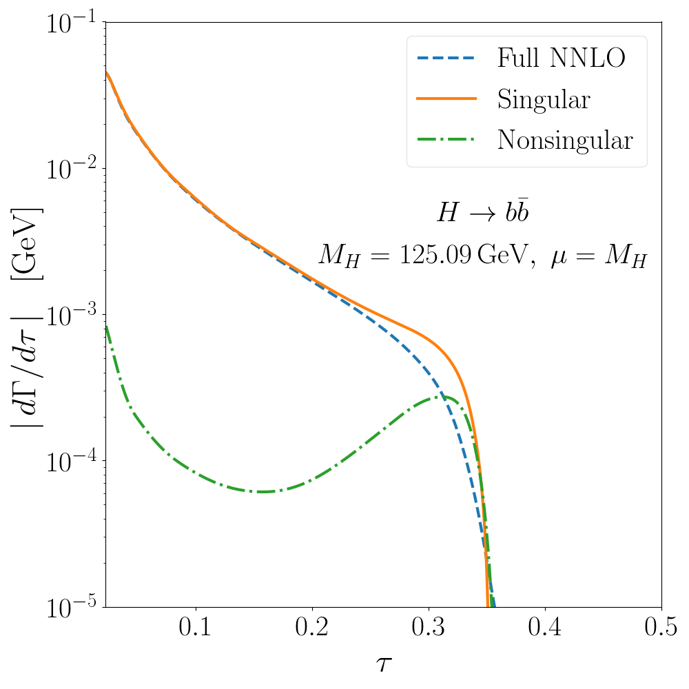
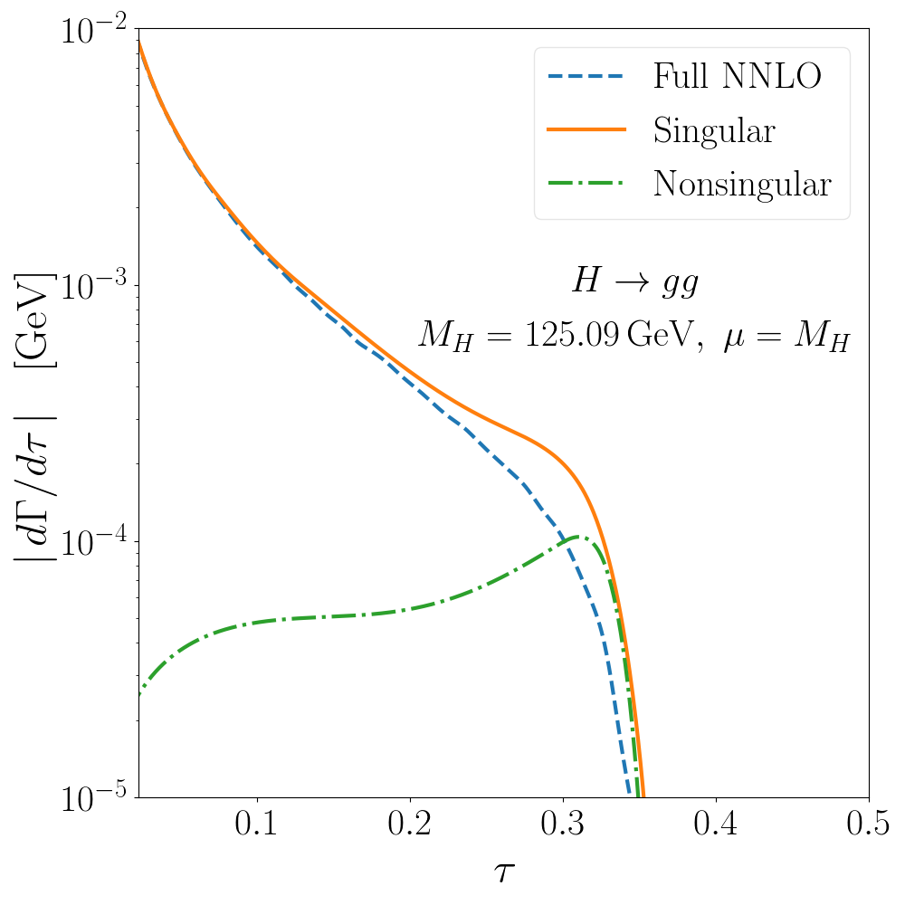
Figure 2: The full, singular and nonsingular contributions to the Higgs boson decay rate as a function of $\tau\equiv\mathcal{T}_{2}/(2M_{H})$. The left panel shows the process $H\rightarrow b\bar{b}$, the right shows $H\rightarrow gg$.

The uncertainties associated with the resummed and fixed-order calculations are estimated by varying the profile scales. For the uncertainty arising from the FO part, we adopt the usual prescription of varying $\mu_{\mathrm{FO}}$ up and down by a factor of 2 and taking the maximal absolute deviation from the central value as a measure of the uncertainty. This preserves everywhere the ratios between the various scales $\mu_{H}$, $\mu_{J}$ and $\mu_{S}$ and so the arguments of the logarithms which are resummed by the RGE factors are unaffected. In the resummed case, we vary the profile scales for $\mu_{J}$ and $\mu_{S}$ about their central profiles while keeping $\mu_{H}=\mu_{\mathrm{FO}}$ fixed. Specifically, defining a variation function (see e.g. Ref. Gangal:2014qda )

$$f_{\mathrm{vary}}(x)=\begin{cases}2(1-x^{2}/x_{3}^{2})&0\leq x\leq x_{3}/2\\ 1+2(1-x/x_{3})^{2}&x_{3}/2\leq x\leq x_{3}\\ 1&x_{3}\leq x\end{cases}\,,$$ (22)

we vary the soft- and jet-function scales such that

$$\mu_{S}^{\uparrow}(x) =f_{\mathrm{vary}}(x)\mu_{S}(x)\,,$$

$$\mu_{S}^{\downarrow}(x) =f_{\mathrm{vary}}(x)^{-1}\mu_{S}(x)\,,$$

$$\mu_{J}^{\uparrow}(x) =\mu_{S}(x)^{1/2-\eta}\mu_{\mathrm{FO}}^{1/2+\eta}\,,$$

$$\mu_{J}^{\downarrow}(x) =\mu_{S}(x)^{1/2+\eta}\mu_{\mathrm{FO}}^{1/2-\eta}\,,$$ (23)

where $\eta=1/6$. In this way the arguments of the resummed logarithms are varied in order to estimate the size of higher-order corrections in the resummed series while maintaining the scale hierarchy $\mu_{\mathrm{FO}}\sim\mu_{H}\gg\mu_{J}\sim\sqrt{\mu_{H}\mu_{S}}\gg\mu_{S}$. More details on the specifics of this prescription may be found in Ref. Gangal:2014qda . In addition, we include two more profiles where we vary all $x_{i}$ transition points by $\pm 0.025$ simultaneously. We thus obtain 6 profile variations in total and take the maximal absolute deviation in the result from the central value as the resummation uncertainty. The total uncertainty is then obtained as the quadrature sum of the resummation and fixed-order uncertainties. The profiles and their variations are shown in fig. 3 for both the $b\bar{b}$ and $gg$ cases.

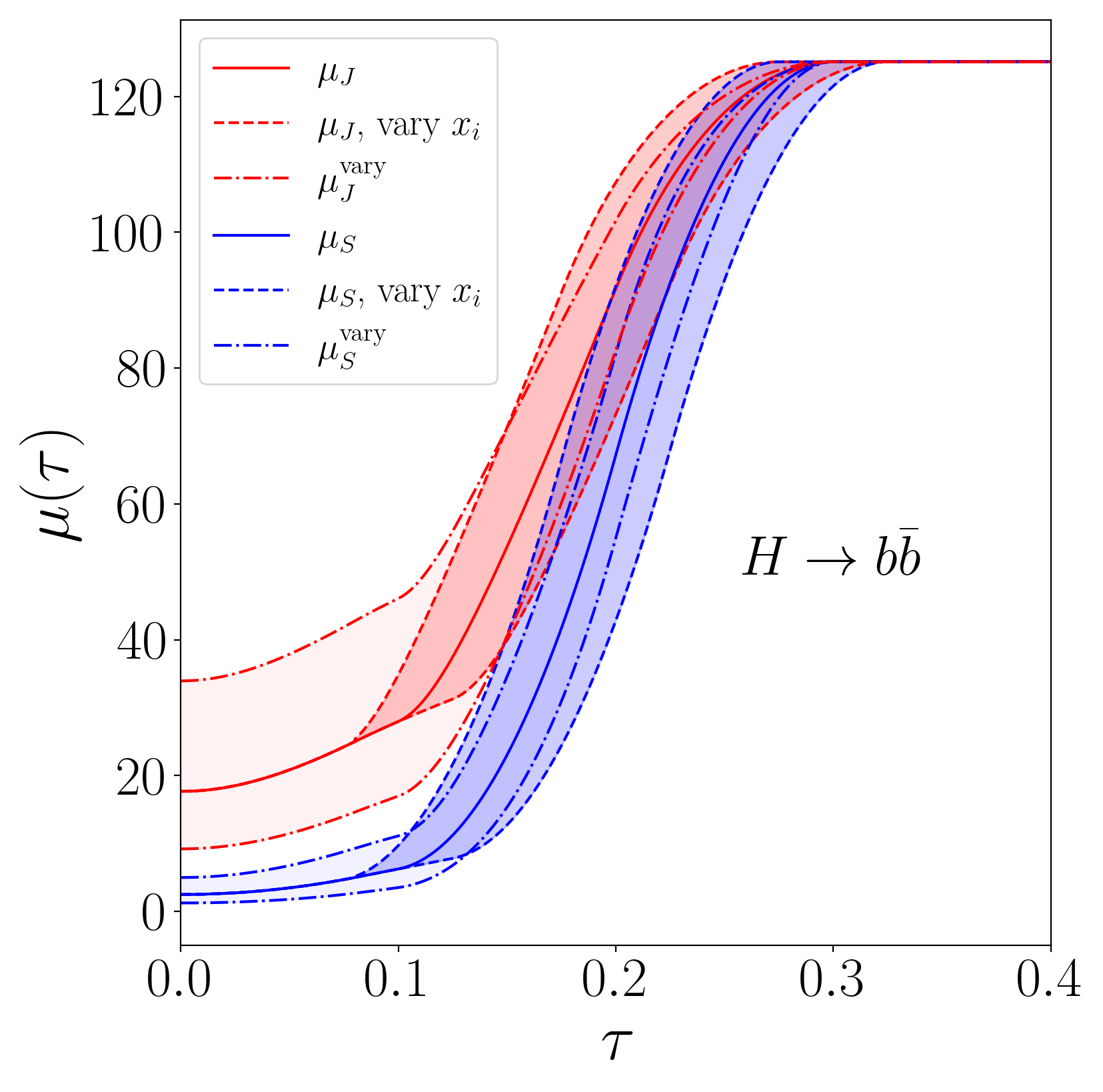
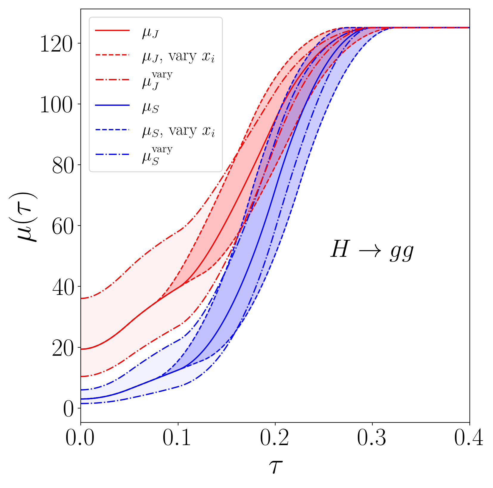
Figure 3: The profile scales from eq. (19) for the $b\bar{b}$ case (left) and $gg$ case (right). The red (blue) curves show the jet (soft) scale $\mu_{J}$ ($\mu_{S}$) and its variations. Variations due to shifts in the transition points $x_{i}$ are shown as dashed lines, while the variations in eq. (23) are shown as dashed-dotted lines. Variations of $\mu_{H}$ result in an overall rescaling of these curves and hence are not shown.

3.2.2 Comparing the spectrum and the derivative of the cumulant

Since the profile scales which we just discussed have themselves a functional dependence on $\mathcal{T}_{2}$, the integral of the spectrum that one obtains from eq. (2.1) is not exactly equal to the cumulant in eq. (3.1) evaluated at the highest scale.

Choosing canonical scaling, i.e. $\mu\propto\mathcal{T}_{2}^{\rm cut}$, we have

$$\int_{0}^{\mathcal{T}_{2}^{\max}}\frac{\mathrm{d}\Gamma^{\mathrm{NNLL}^{\prime}}}{\mathrm{d}\Phi_{2}\mathrm{d}\mathcal{T}_{2}}(\mu(\mathcal{T}_{2}))\mathrm{d}\mathcal{T}_{2}=\frac{\mathrm{d}\Gamma^{\mathrm{NNLL}^{\prime}}}{\mathrm{d}\Phi_{2}}(\mathcal{T}_{2}^{\max},\mu(\mathcal{T}_{2}^{\max}))+\mathcal{O}(\rm N^{3}LL)\,,$$ (24)

where ${\mathcal{T}_{2}^{\max}}$ is the upper kinematical limit. By integrating the spectrum we therefore obtain not only the cumulant but also unwanted additional terms of higher order. Depending on the convergence properties of the perturbative series, these additional terms can be numerically relevant and cause a sizeable difference between the inclusive decay rate obtained from the resummed calculation and the FO result. To obviate this problem, we supplement the spectrum in eqs. (3.1) and (3.1) with an additional higher order term. The contribution of this term is restricted to the region of $\mathcal{T}_{2}$ where the spurious $\rm N^{3}LL$ terms are sizeable, and vanishes in the FO region; crucially, upon integration it ensures that the FO rate is recovered. It takes the form:

$$\kappa(\mathcal{T}_{2})\left[\frac{\mathrm{d}}{\mathrm{d}\mathcal{T}_{2}}\frac{\mathrm{d}\Gamma^{\rm NNLL^{\prime}}}{\mathrm{d}\Phi_{2}}(\mathcal{T}_{2},\mu_{h}(\mathcal{T}_{2}))-\frac{\mathrm{d}\Gamma^{\rm NNLL^{\prime}}}{\mathrm{d}\Phi_{2}\mathrm{d}\mathcal{T}_{2}}(\mu_{h}(\mathcal{T}_{2}))\right],$$ (25)

where $\kappa(\mathcal{T}_{2})$ and $\mu_{h}(\mathcal{T}_{2})$ are smooth functions. It is clear that this vanishes in the FO region where $\mu_{h}(\mathcal{T}_{2})\sim M_{H}$ as required – in order to restrict its contribution further, we also choose $\kappa(\mathcal{T}_{2})$ to tend to zero in this region to minimise its size before exact cancellation is reached and choose the profile scale $\mu_{h}(\mathcal{T}_{2})$ to reach $M_{H}$ at a lower value of $\mathcal{T}_{2}$ than the rest of the calculation. This prevents the accuracy of the tail of the spectrum from being spoiled, while keeping the resulting changes in the peak region contained within its scale uncertainty band. We tune $\kappa(\mathcal{T}_{2})$ to recover the correct inclusive rate, both for the central FO scale and also for its variations such that the result of integration is identical to a FO calculation for inclusive quantities.

3.2.3 Power-suppressed corrections to the nonsingular cumulant

The integration of the differential decay rate in eq. (3.1) over the $\Phi_{2}$ phase space produces an NNLO accurate total width. For differential quantities, however, the $\mathcal{O}(\alpha_{\rm s}^{2})$ terms in eq. (3.1) are guaranteed to be NNLO accurate only up to power corrections in $\mathcal{T}_{2}^{\mathrm{cut}}$ since any projective map one could devise could not preserve all $\Phi_{2}$ quantities simultaneously. This fundamental limit on the accuracy of event generators actually allows us to sidestep the problem of implementing a full NNLO subtraction – since the total width is the only quantity that is certain to be NNLO accurate, we can drop all the $\mathcal{O}(\alpha_{\rm s}^{2})$ terms in the cumulant and achieve the correct NNLO width by reweighting. That is, rather than implementing the full form of eq. (3.1), we instead use

$$\frac{\widetilde{\mathrm{d}\Gamma^{\textsc{mc}}_{2}}}{\mathrm{d}\Phi_{2}}(\mathcal{T}_{2}^{\mathrm{cut}}) =\frac{\mathrm{d}\Gamma^{\rm NNLL^{\prime}}}{\mathrm{d}\Phi_{2}}(\mathcal{T}_{2}^{\mathrm{cut}})-\biggl{[}\frac{\mathrm{d}\Gamma^{\rm NNLL^{\prime}}}{\mathrm{d}\Phi_{2}}(\mathcal{T}_{2}^{\mathrm{cut}})\biggr{]}_{\rm NLO_{2}}+B_{2}(\Phi_{2})+V_{2}(\Phi_{2})$$

$$\quad+\int\!\frac{\mathrm{d}\Phi_{3}}{\mathrm{d}\Phi_{2}}\,B_{3}(\Phi_{3})\,\theta\left(\mathcal{T}_{2}(\Phi_{3})<\mathcal{T}_{2}^{\mathrm{cut}}\right)\,,$$ (26)

which requires only a local NLO subtraction. The remaining nonsingular terms take the form

$$\frac{\mathrm{d}\Gamma_{2}^{\mathrm{nons}}}{\mathrm{d}\Phi_{2}}(\mathcal{T}_{2}^{\mathrm{cut}}) =\bigl{[}\alpha_{\rm s}f_{1}(\mathcal{T}_{2}^{\mathrm{cut}},\Phi_{2})+\alpha_{\rm s}^{2}f_{2}(\mathcal{T}_{2}^{\mathrm{cut}},\Phi_{2})\bigr{]}\mathcal{T}_{2}^{\mathrm{cut}}$$ (27)

where the functions $f_{i}(\mathcal{T}_{2}^{\rm cut},\Phi_{2})$ are at worst logarithmically divergent in the small $\mathcal{T}_{2}^{\mathrm{cut}}$ limit. We include the NLO term proportional to $f_{1}(\mathcal{T}_{2}^{\mathrm{cut}},\Phi_{2})$ in eq. (26) via an on-the-fly $\mathrm{NLO}_{2}$ calculation, but neglect the $f_{2}(\mathcal{T}_{2}^{\mathrm{cut}},\Phi_{2})$ piece. The size of this neglected term as a function of the cut is shown in fig. 4 for both processes. We see that at our default value of $\mathcal{T}_{2}^{\mathrm{cut}}=1\,\mathrm{GeV}$ the missing $\mathcal{O}(\alpha_{\rm s}^{2})$ terms are of a size $\sim 10^{-5}~{}\,\mathrm{GeV}$ in both cases. This amounts to a relative correction of $\mathcal{O}(0.4\%)$ for the $b\bar{b}$ channel and of $\mathcal{O}(1\%)$ for the $gg$. Smaller power corrections could naturally also be obtained by modifying the factorisation formula eq. (3) to include subleading power contributions Moult:2019mog ; Moult:2018jjd or by lowering further the value of $\mathcal{T}_{2}^{\mathrm{cut}}$. In this limit, however, the calculation suffers from numerical problems originating from the stability of the matrix elements and of the NLO subtraction procedure close to extreme soft or collinear configurations, which motivates our default choice.

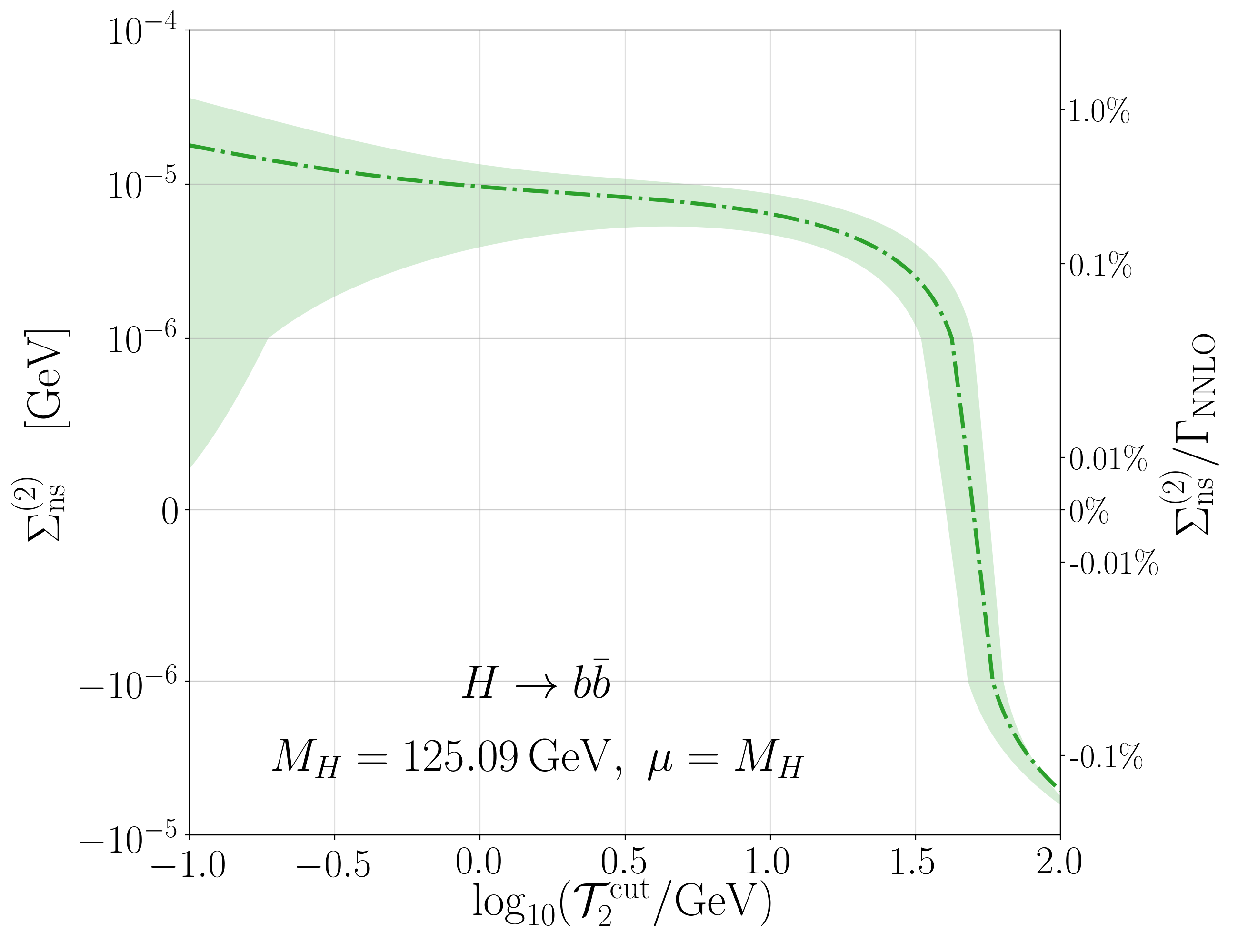
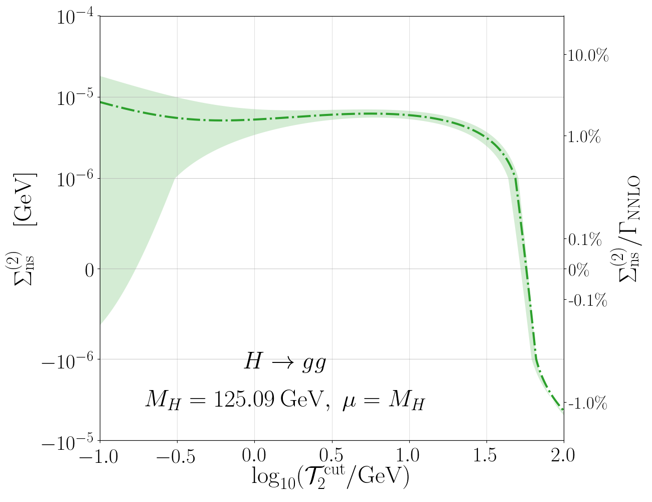
Figure 4: The missing $\mathcal{O}(\alpha_{\rm s}^{2})$ nonsingular contribution to the cumulant as a function of $\mathcal{T}_{2}^{\mathrm{cut}}$ for the $H\to b\bar{b}$ process (left) and the $H\to gg$ (right). The shaded band denotes the statistical error on the spectrum rather than the cumulant, which we include to help gauge the size of the uncertainty on the power corrections as a function of $\mathcal{T}_{2}^{\mathrm{cut}}$.

In order to correct for this discrepancy and obtain the correct NNLO inclusive decay width, we may simply rescale the weights of the $\Phi_{2}$ events in such a way that we match the known analytic result at NNLO. We are thus able to include the effects of the $f_{2}$ term in eq. (27) on the total cross section that would have been present had we implemented eq. (3.1) literally. Since neither eq. (3.1) nor our approach in eq. (26) achieves the exact $\mathcal{O}(\alpha_{\rm s}^{2})$ $\Phi_{2}$ dependence of all observables, our approximation does not inherently limit the accuracy of our predictions.

3.2.4 Interface to the parton shower

We briefly recap the main features of the parton shower interface in Geneva here and refer the interested reader to section 3 of Ref. Alioli:2015toa for a more detailed discussion.

The partonic jet decay rates $\mathrm{d}\Gamma^{\textsc{mc}}_{2}$, $\mathrm{d}\Gamma^{\textsc{mc}}_{3}$ and $\mathrm{d}\Gamma^{\textsc{mc}}_{\geq 4}$ each include contributions from higher multiplicity phase space points, but only in those cases where $\mathcal{T}_{N}(\Phi_{M})<\mathcal{T}_{N}^{\mathrm{cut}}$. In order to make the calculation fully differential in the higher multiplicities, a parton shower is interfaced which adds radiation to each jet decay rate in a unitary and recursive manner. Ideally, the shower should leave the values of the jet rates and their accuracy unaffected, restoring the emissions in $\mathrm{d}\Gamma^{\textsc{mc}}_{2}$ and $\mathrm{d}\Gamma^{\textsc{mc}}_{3}$ which were integrated over when the jet rates were constructed and also adding extra final-state partons to the inclusive $\mathrm{d}\Gamma^{\textsc{mc}}_{\geq 4}$.

For illustrative purposes, we consider a shower strongly ordered in $\mathcal{T}_{N}$, such that $\mathcal{T}_{2}(\Phi_{3})\gg\mathcal{T}_{3}(\Phi_{4})\gg\dots$ A shower history of this kind could be constructed by taking the output of a shower ordered in a more conventional variable and reclustering the partons using the $N$-jettiness metric $\mathcal{T}_{N}$.

In general, the requirement of the preservation of the accuracy of the jet rates after applying the shower on a phase space point $\Phi_{N}$ sets constraints on the point $\Phi_{M}$ reached after the shower. For the cases in which the showered events originate from $\Phi_{2}$ events, the main constraint is that the integral of the decay rate below the $\mathcal{T}_{2}^{\mathrm{cut}}$ (which is NNLL^′+NNLO accurate) must not be modified. The emissions generated by the shower must in this case satisfy $\mathcal{T}_{2}(\Phi_{N})<\mathcal{T}_{2}^{\mathrm{cut}}$, so that they recover the events which were integrated over in the construction of the 2-jet exclusive decay rate and add events with more emissions below the cut. In case of a single shower emission we require also that the resulting $\Phi_{3}$ point is projectable onto $\Phi_{2}$, as these are the only configurations at this order which are included in eq. (26). Both of these conditions can be implemented with a careful choice of the starting scale of the shower. The preservation of the decay rate below the cut is then ensured by the unitarity of the shower evolution. In practice, we allow for a tiny spillover up to $5\%$ above $\mathcal{T}_{2}^{\mathrm{cut}}$ in order to smoothen the transition.

The showering of $\Phi_{3}$ and $\Phi_{4}$ events must be treated more carefully in order to preserve the NNLL^′+NNLO accuracy of the $\mathcal{T}_{2}$ spectrum. Crucially, we must ensure that the $\Phi_{4}$ points produced after the first emission are projectable onto $\Phi_{3}$ using the $\mathcal{T}_{2}$-preserving map discussed in App. A. Since the shower cannot guarantee this, we instead perform the first emission in Geneva (using the analytic form of the LL Sudakov factor and phase space maps) and only thereafter allow the shower to act as usual, subject to the restriction $\mathcal{T}_{4}(\Phi_{N})\leq\mathcal{T}_{3}(\Phi_{4})$. We apply this procedure only to the $\Phi_{3}$ events and find that

$$\frac{\mathrm{d}\Gamma_{3}^{\mathrm{MC}}}{\mathrm{d}\Phi_{3}}(\mathcal{T}_{2}>\mathcal{T}_{2}^{\mathrm{cut}},\mathcal{T}_{3}^{\mathrm{cut}},\Lambda_{3}) =\frac{\mathrm{d}\Gamma^{\textsc{mc}}_{3}}{\mathrm{d}\Phi_{3}}(\mathcal{T}_{2}>\mathcal{T}_{2}^{\mathrm{cut}},\mathcal{T}_{3}^{\mathrm{cut}})\,U_{3}(\mathcal{T}_{3}^{\mathrm{cut}},\Lambda_{3})$$ (28)

$$\frac{\mathrm{d}\Gamma_{\geq 4}^{\mathrm{MC}}}{\mathrm{d}\Phi_{4}}(\mathcal{T}_{2}>\mathcal{T}_{2}^{\mathrm{cut}},\mathcal{T}_{3}^{\mathrm{cut}},\mathcal{T}_{3}>\Lambda_{3})=\frac{\mathrm{d}\Gamma^{\textsc{mc}}_{\geq 4}}{\mathrm{d}\Phi_{4}}(\mathcal{T}_{2}>\mathcal{T}_{2}^{\mathrm{cut}},\mathcal{T}_{3}>\mathcal{T}_{3}^{\mathrm{cut}})$$ (29)

$$\quad+\frac{\mathrm{d}}{\mathrm{d}\mathcal{T}_{3}}\,\frac{\mathrm{d}\Gamma^{\mathrm{MC}}_{3}}{\mathrm{d}\Phi_{3}}(\mathcal{T}_{2}>\mathcal{T}_{2}^{\mathrm{cut}},\mathcal{T}_{3}^{\mathrm{cut}},\mathcal{T}_{3})\times\mathcal{P}(\Phi_{4})\,\theta(\Lambda_{3}<\mathcal{T}_{3}<\mathcal{T}_{3}^{\max})\,.$$

By choosing $\Lambda_{3}\sim\Lambda_{\mathrm{QCD}}$, the Sudakov factor $U_{3}(\mathcal{T}_{3}^{\mathrm{cut}},\Lambda_{3})$ becomes vanishingly small and we can relax the shower conditions on the $3$-jet contributions. The showered events therefore originate almost exclusively from either $\mathrm{d}\Gamma^{\textsc{mc}}_{2}$ or $\mathrm{d}\Gamma^{\textsc{mc}}_{\geq 4}$.

We choose starting scales of $\mathcal{T}_{2}^{\mathrm{cut}}$ and $\mathcal{T}_{3}^{\mathrm{cut}}$ for the $\Phi_{2}$ and $\Phi_{3}$ events respectively. For the $\Phi_{4}$ events, the starting scale $t$ needs to be a measure of the hardness of the splitting, for example the $3$-jettiness value $\mathcal{T}_{3}$. Here we follow the choice made in Ref. Bizon:2019tfo and set

$$t=2p_{\mathrm{daughter}}\cdot p_{\mathrm{sister}}\frac{E_{\mathrm{daughter}}}{E_{\mathrm{sister}}}\,,$$ (30)

where the energies are defined in the Higgs boson rest frame. After interfacing to the Pythia8 parton shower, we expect the accuracy for observables other than $\mathcal{T}_{2}$ to be no worse than that of the standalone Pythia8 shower.

3.2.5 Nonperturbative power corrections and hadronisation

The approach described up to now does not take into account nonperturbative power corrections, which can significantly affect the partonic predictions. The framework of SCET allows these nonperturbative effects to be systematically included via the introduction of a shape function $f(k,\mu)$ modifying the soft component as Korchemsky:1999kt ; Hoang:2007vb ; Ligeti:2008ac

$$S_{2}(\mathcal{T}_{2},\mu)=\int\mathrm{d}k\,S_{2}^{\rm pert}(\mathcal{T}_{2}-k,\mu)\,f(k,\mu),$$ (31)

where $S_{2}^{\rm pert}$ is the perturbative soft function. At small $\mathcal{T}_{2}\sim\Lambda_{\mathrm{QCD}}$ the shape function gives an $\mathcal{O}(1)$ contribution to the cross section, while for larger $\mathcal{T}_{2}$ values one can show that the dominant contribution is of $\mathcal{O}(\Lambda_{\mathrm{QCD}}/\mathcal{T}_{2})$ and results in a overall shift of the $\mathcal{T}_{2}$ spectrum Abbate:2010xh . The same conclusions can be reached using a dispersive model and an effective value for the strong coupling constant in the nonperturbative regime Dokshitzer:1995zt ; Dokshitzer:1995qm ; Dokshitzer:1998kz ; Gehrmann:2012sc .

The resummed predictions obtained by Geneva at the partonic level only include the perturbative soft function, and we delegate the provision of nonperturbative ingredients to the hadronisation models used in Pythia8. Therefore, after the showering stage, the events are interfaced to the phenomenological hadronisation model in Pythia8 without further constraints on the kinematics of the hadronised event. This means that the hadronisation can potentially cause significant shifts of the $\mathcal{T}_{2}$ spectrum.

It is known that the $2$-jettiness and the thrust observables receive different hadronisation corrections, due to the different treatment of the hadron masses in their definitions Salam:2001bd ; Mateu:2012nk . Since there are currently no experimental data with which we can compare for these decay channels, in this work we consistently use the definition of $\mathcal{T}_{2}$ in eq. (1) even for hadronised events, despite the larger power corrections compared to schemes with a different mass treatment. This is different from the approach taken for the $e^{+}e^{-}\to$ jets study in Ref. Alioli:2012fc , where the definition based on thrust was used to compare to LEP data.

It is important to notice that we do not include uncertainties from these nonperturbative contributions in the results presented in the next section. In our approach, a crude estimate of their size could in principle be obtained by varying the tune parameters of the Pythia8 hadronisation model, but a more detailed study of this goes beyond the scope of this work. It is worth noting, however, that in any calculation obtained by matching higher-order calculations with parton shower one has to carefully evaluate which parameters are truly encoding nonperturbative effects and should therefore be tuned.

4 Results

In this section we present the full Geneva results obtained by matching the resummed calculation to the fixed order. We adopt the same values of SM parameters as in sec. 2.2 and set $\mathcal{T}_{2}^{\mathrm{cut}}=\mathcal{T}_{3}^{\mathrm{cut}}=1\,\mathrm{GeV}$. We interface to the Pythia8 generator which showers our events and use the $e^{+}e^{-}$ tune 3, turn off QED effects and prevent the decay of $b$-hadrons. We set the strong coupling used by Pythia8 to $\alpha_{\rm s}=0.118$, although ideally, one should perform a dedicated tune to accommodate for this change.

With the setup as described, we verified that we obtain the correct NNLO decay rate up to the power corrections shown in fig. 4. The partonic results are presented for each channel in Tab. 1, where the analytic values have been obtained using the formulae appearing in App. B.

$\Gamma^{i}_{\mathrm{NNLO}}(\mu)/\,\mathrm{GeV}$	Analytic	Geneva, $\mathcal{T}_{2}^{\mathrm{cut}}=1\,\mathrm{GeV}$
$i=b,\,\mu=M_{H}$	$3.053\text{\times}{10}^{-3}$	$3.042\text{\times}{10}^{-3}$$\pm$$0.2\text{\times}{10}^{-5}$
$i=b,\,\mu=2M_{H}$	$3.104\text{\times}{10}^{-3}$	$3.094\text{\times}{10}^{-3}$$\pm$$0.2\text{\times}{10}^{-5}$
$i=b,\,\mu=M_{H}/2$	$2.973\text{\times}{10}^{-3}$	$2.961\text{\times}{10}^{-3}$$\pm$$0.2\text{\times}{10}^{-5}$
$i=g,\,\mu=M_{H}$	$3.374\text{\times}{10}^{-4}$	$3.338\text{\times}{10}^{-4}$$\pm$$1.2\text{\times}{10}^{-6}$
$i=g,\,\mu=2M_{H}$	$3.189\text{\times}{10}^{-4}$	$3.178\text{\times}{10}^{-4}$$\pm$$0.8\text{\times}{10}^{-6}$
$i=g,\,\mu=M_{H}/2$	$3.491\text{\times}{10}^{-4}$	$3.407\text{\times}{10}^{-4}$$\pm$$1.8\text{\times}{10}^{-6}$

Table 1: Comparison of Higgs boson partial widths obtained from NNLO analytic expressions and at the partonic level from Geneva. Note that, due to the presence of the power corrections displayed in fig. 4, the values do not agree exactly within the statistical error and therefore a reweighting must be performed.

In general, the Geneva method also guarantees NNLO accuracy for distributions differential in the Born variables of the process (see for example Ref. Alioli:2019qzz ). In the case of a spin-0 boson decaying into two particles, however, the Born phase space is parameterised by only two angles and is flat in both – there is therefore no non-trivial shape information which can be compared to a fixed-order calculation. We have, however, validated our NLO calculations of $H\rightarrow b\bar{b}g$ and $H\rightarrow ggg$/$H\rightarrow q\bar{q}g$ against aMC@NLO Alwall:2014hca and found perfect agreement. We checked that by increasing the $\mathcal{T}_{2}^{\mathrm{cut}}$ to $\sim 5$ GeV we obtain smaller power corrections (see fig. 4) – however, since this would limit our higher-order resummed predictions for the shape of the spectrum to $\mathcal{T}_{2}>5\,\mathrm{GeV}$, in the following we continue to use $\mathcal{T}_{2}^{\mathrm{cut}}=1\,\mathrm{GeV}$ and accordingly reweight our events in order to obtain the correct total decay width.

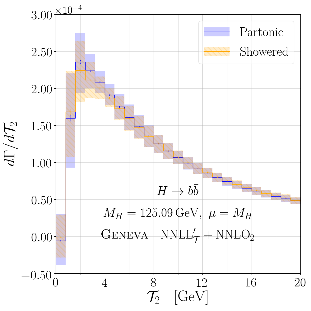
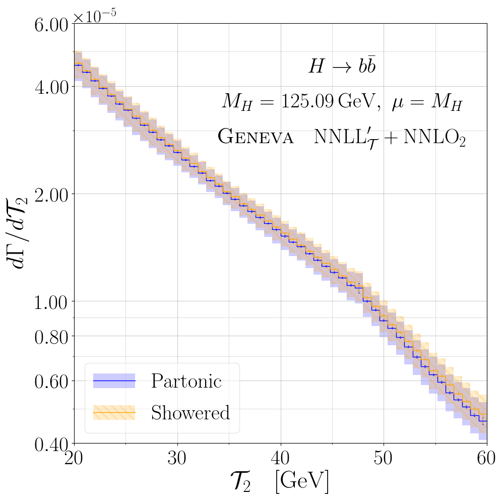
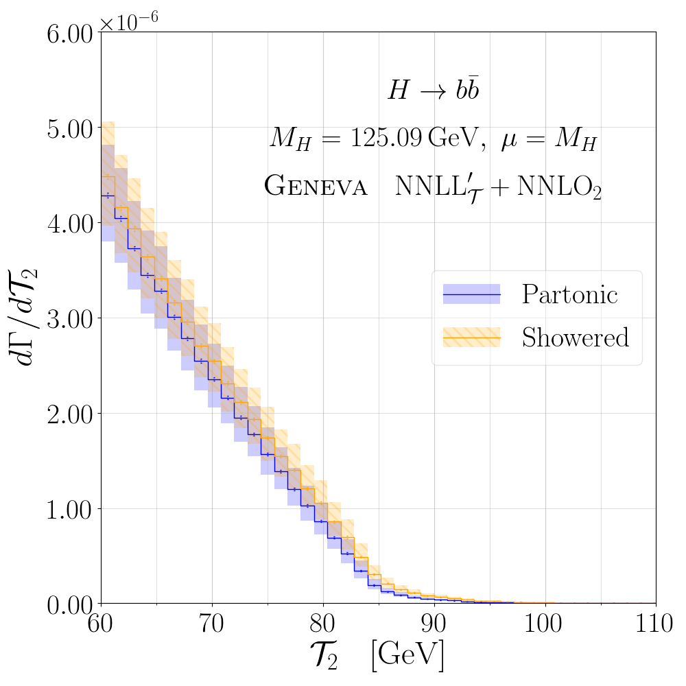
Figure 5: Validation of the $\mathcal{T}_{2}$ spectrum in Geneva for $H\rightarrow b\bar{b}$. The partonic NNLL^′+NNLO $\mathcal{T}_{2}$ resummation is compared to the showered results, before the addition of nonperturbative effects.

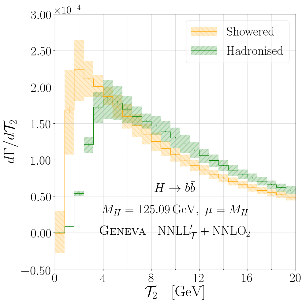
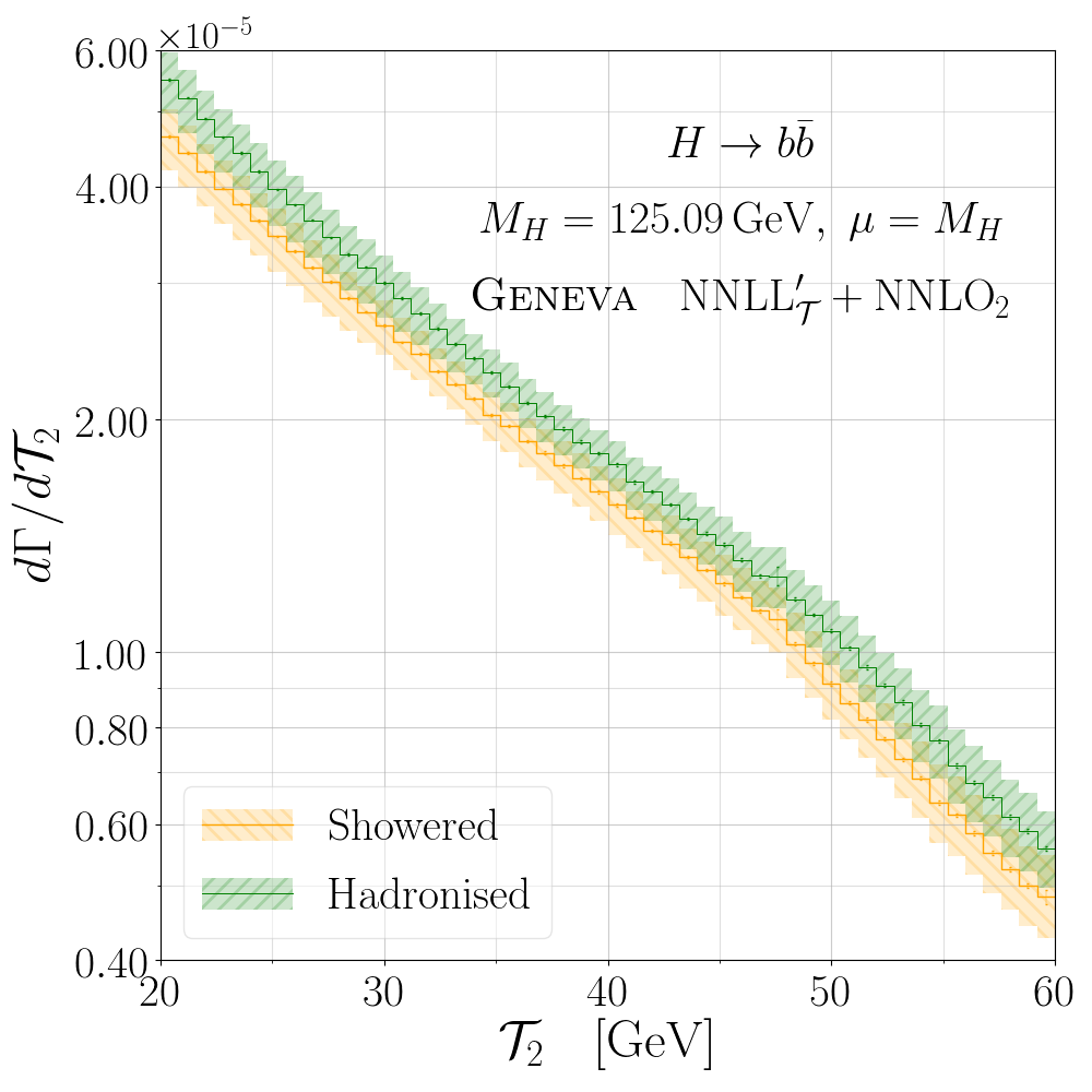
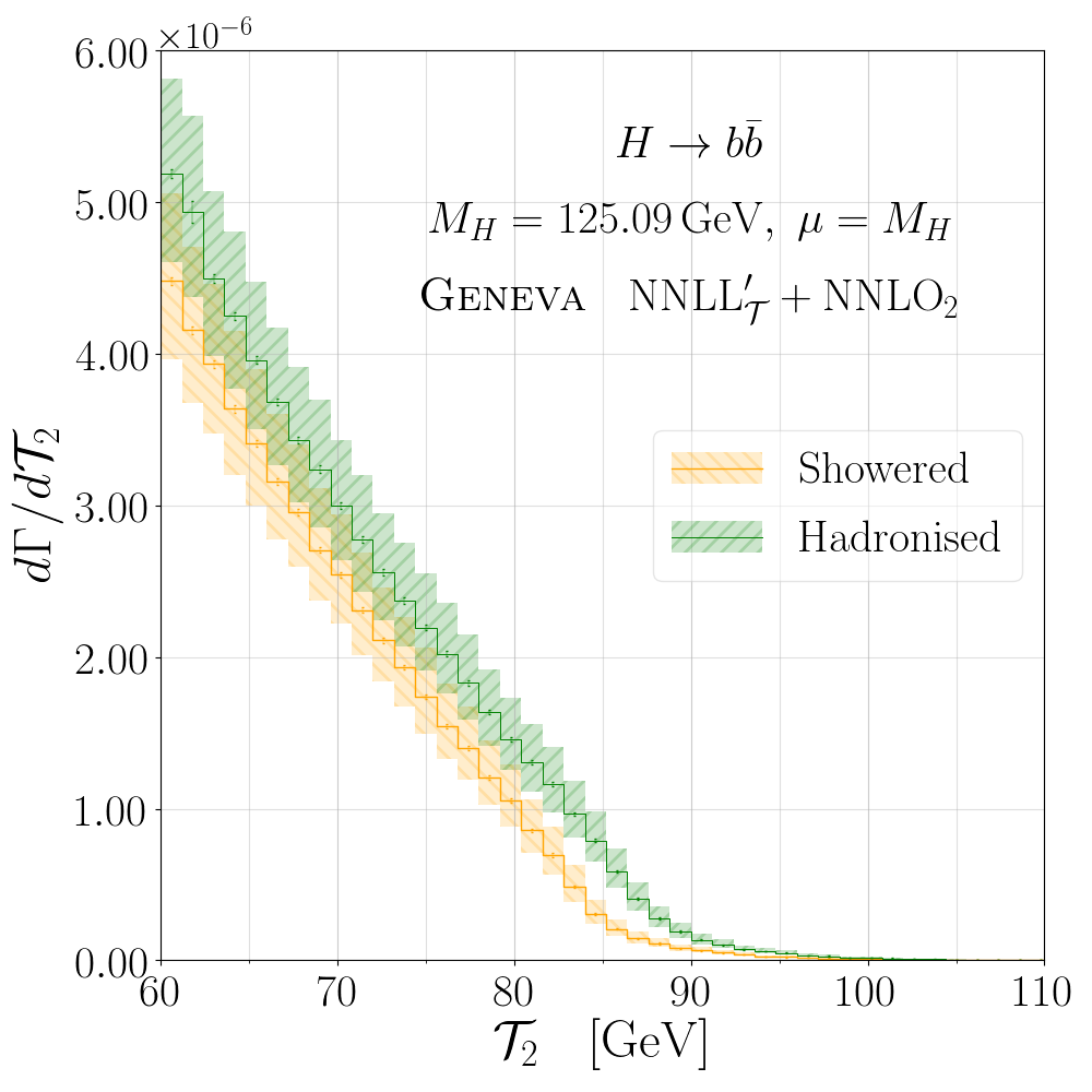
Figure 6: Comparison of the showered and hadronised $\mathcal{T}_{2}$ spectra in Geneva for $H\rightarrow b\bar{b}$.

A comparison of the NNLO+NNLL^′ results at the partonic and showered levels is presented in fig. 6 for the $H\rightarrow b\bar{b}$ process and in fig. 8 for the $H\rightarrow gg$ process, while the corresponding comparisons of the showered and hadronised events are shown in figs. 6 and 8. The panels in the plots show three different regions of the $2$-jettiness spectrum: the peak (leftmost panels), where resummation effects are expected to be dominant; the transition (centre panels), where the resummed and fixed-order calculations compete for importance; and the tail (rightmost panels), where the resummation is switched off and the fixed-order calculation provides the correct physical description. We observe that in the $b\bar{b}$ channel the $\mathcal{T}_{2}$ is well preserved by the shower, while hadronisation effects shift the distribution to higher values of $\mathcal{T}_{2}$ across all regions. This can be compared to the results obtained in Ref. Alioli:2012fc , keeping in mind the aforementioned difference between the $2$-jettiness definitions used at hadron level and the different energy scale which result in competing contributions to the shift.

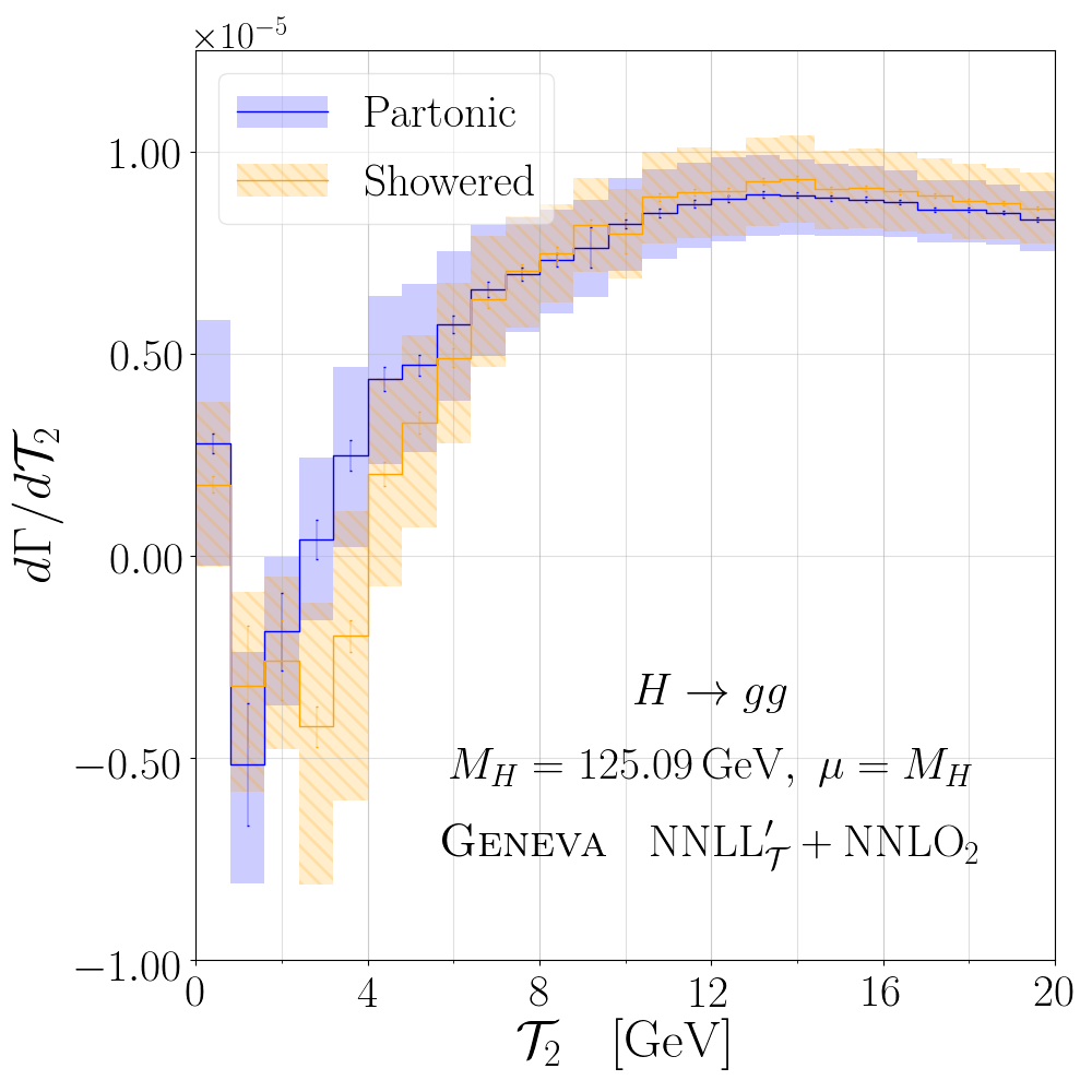
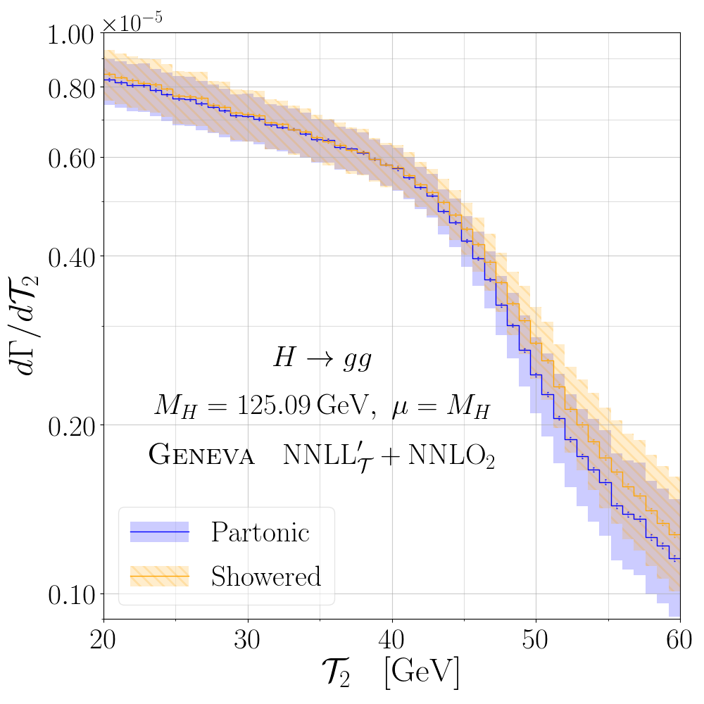
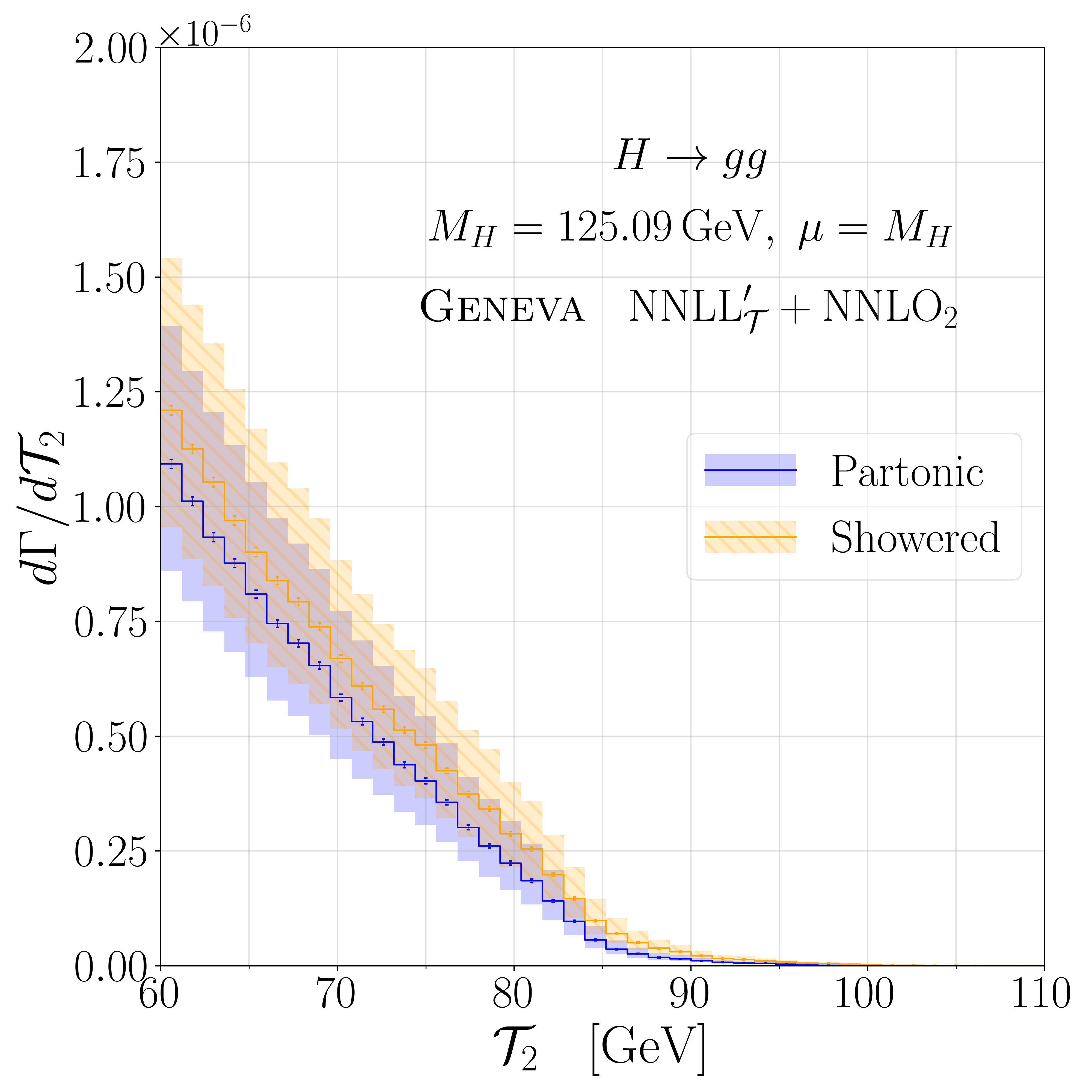
Figure 7: Validation of the $\mathcal{T}_{2}$ spectrum in Geneva for $H\rightarrow gg$. The partonic NNLL^′+NNLO $\mathcal{T}_{2}$ resummation is compared to the showered results, before the addition of nonperturbative effects.

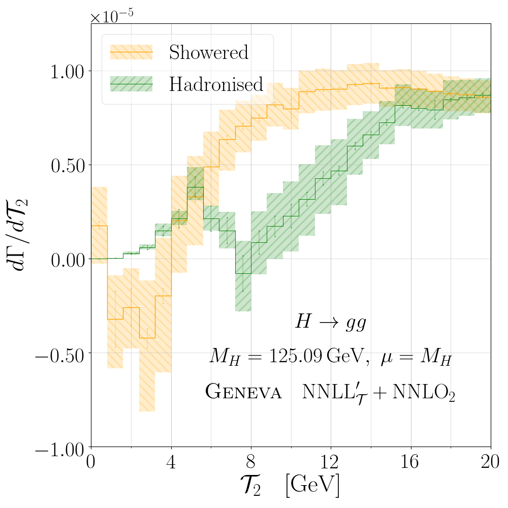
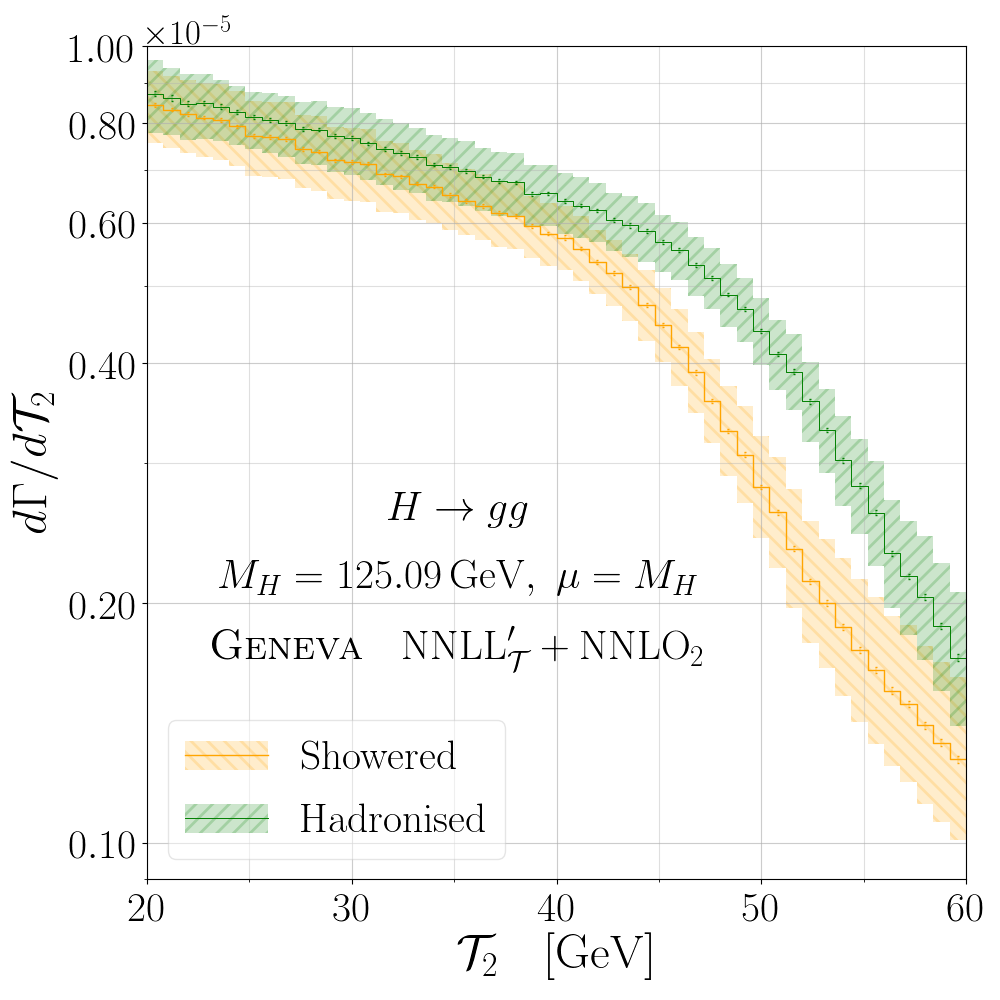
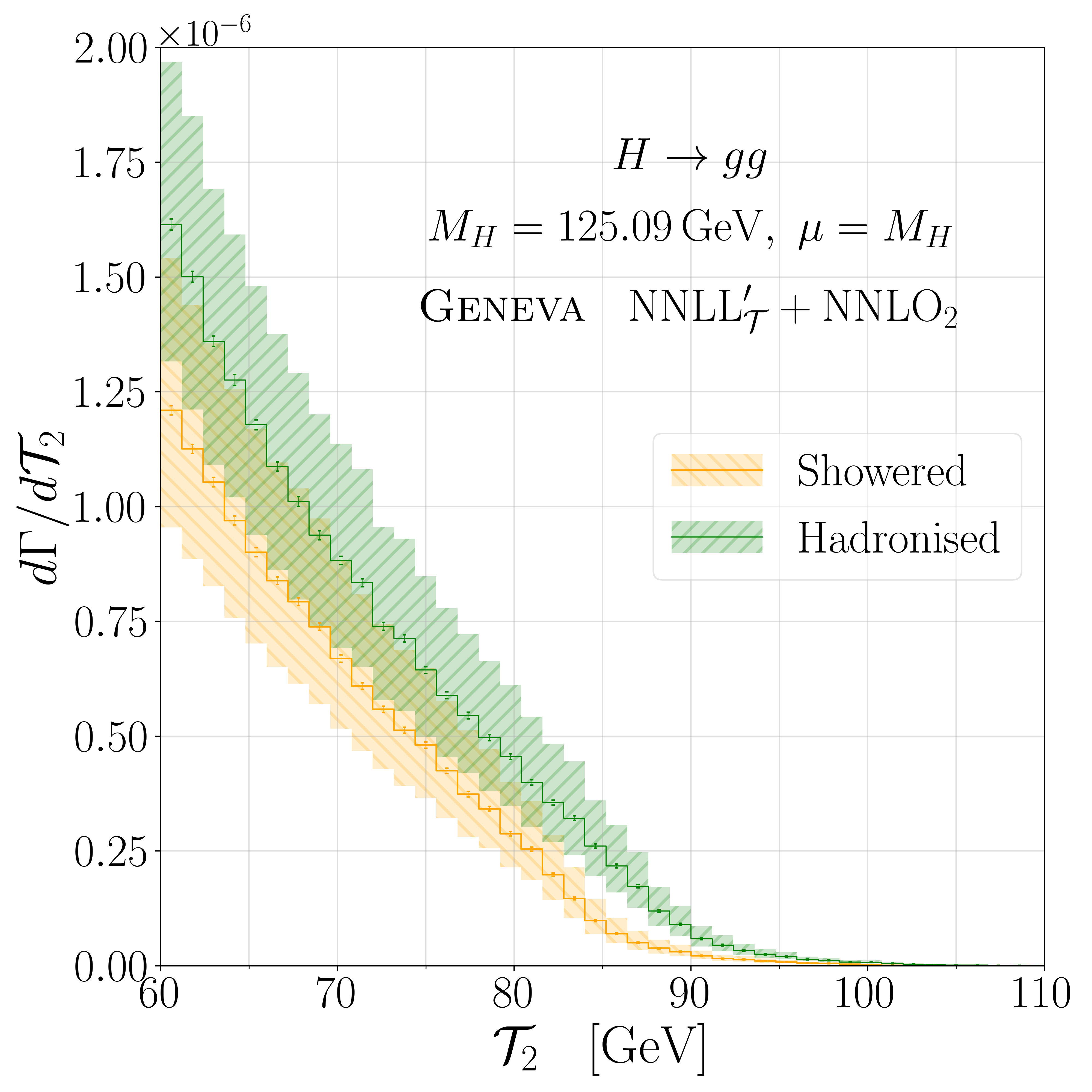
Figure 8: Comparison of the showered and hadronised $\mathcal{T}_{2}$ spectra in Geneva for $H\rightarrow gg$.

In the $gg$ channel, the effect of the shower on the $\mathcal{T}_{2}$ spectrum is greater, especially at the lowest values of $\mathcal{T}_{2}$, but it preserves the shape of the distribution to within the scale variation bands closer to the peak and in the transition region. We also notice that the partonic and showered predictions give a negative cross section for very small values of $\mathcal{T}_{2}$, below the nonperturbative freeze-out of the profile scales. This behaviour should not be concerning as it happens in a region where the perturbative resummed results are already questionable and, as mentioned before, we do not include any nonperturbative uncertainty. We have verified that the size of the negative value is augmented by the nonsingular corrections which we include via an additive approach. Indeed, when examining the resummed $\mathcal{T}_{2}$ distribution alone, the behaviour at small $\mathcal{T}_{2}$ remains negative but is compatible with a value of zero to within the quoted uncertainties.

A peculiar feature is observed in the first bin of fig. 8, which contains the cross section below $\mathcal{T}_{2}^{\rm cut}$ and is positive. This is again a consequence of the missing nonsingular corrections in eq. (26), which are included by the reweighting procedure. Since these are particularly large for this process, see fig. 4, their effect is to change the sign of the cumulant below $\mathcal{T}_{2}^{\rm cut}$.

We also observe somewhat larger effects on the spectrum due to hadronisation compared to the $b\bar{b}$ case, particularly in the peak region. The seemingly unusual behaviour at small $\mathcal{T}_{2}$ is a consequence of the already discussed shift of the spectrum after hadronisation resulting in a smearing of the first bin. We stress again that the small error bands reported are due to the lack of nonperturbative uncertainties.

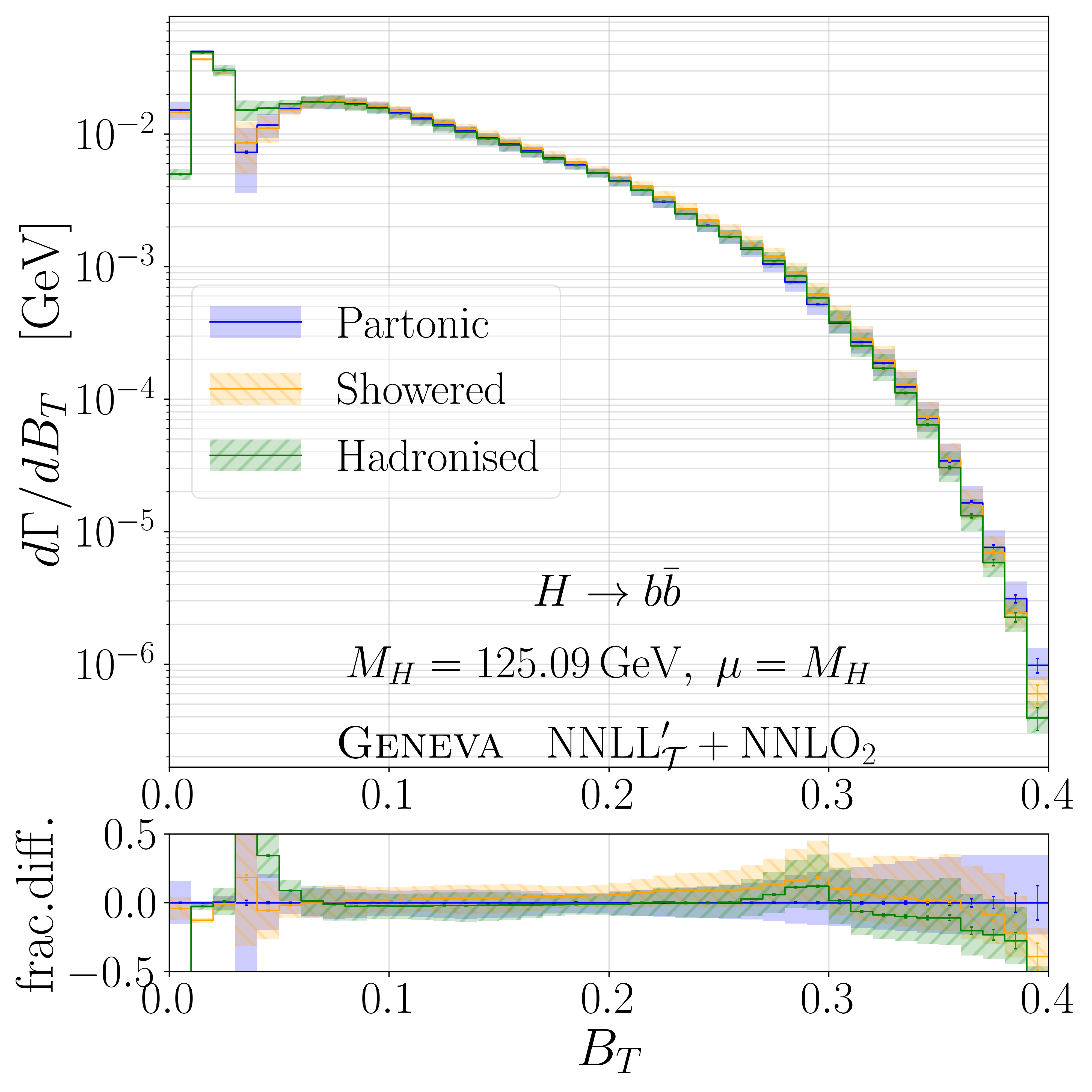
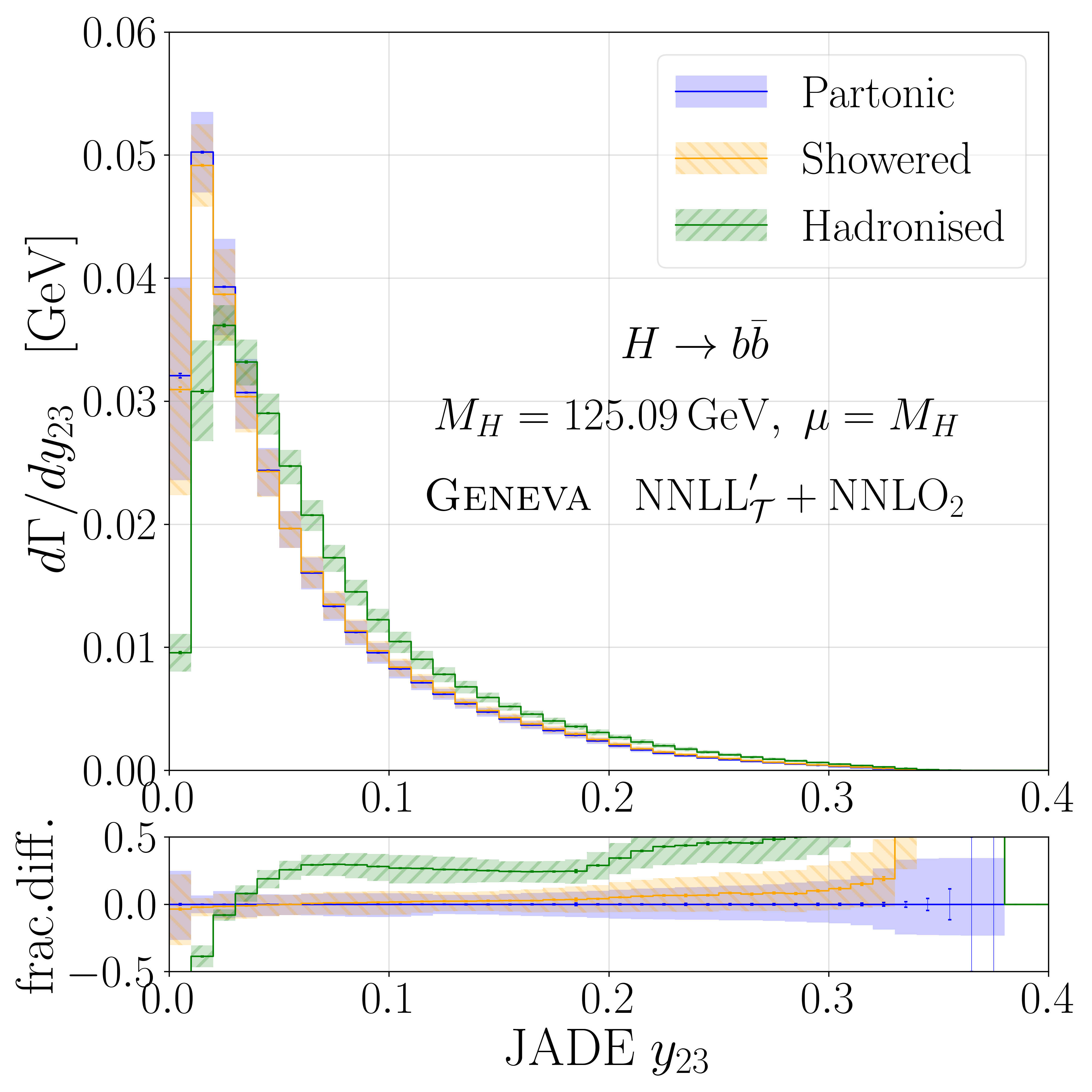
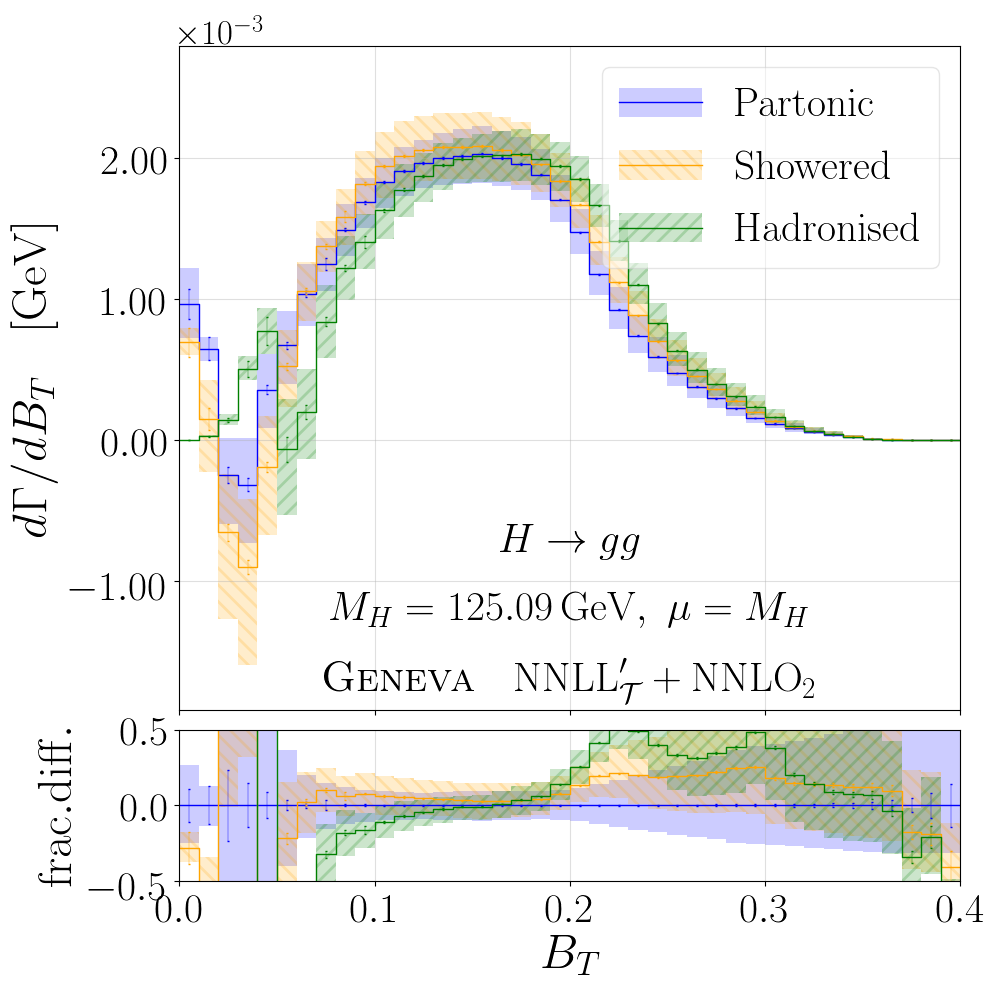
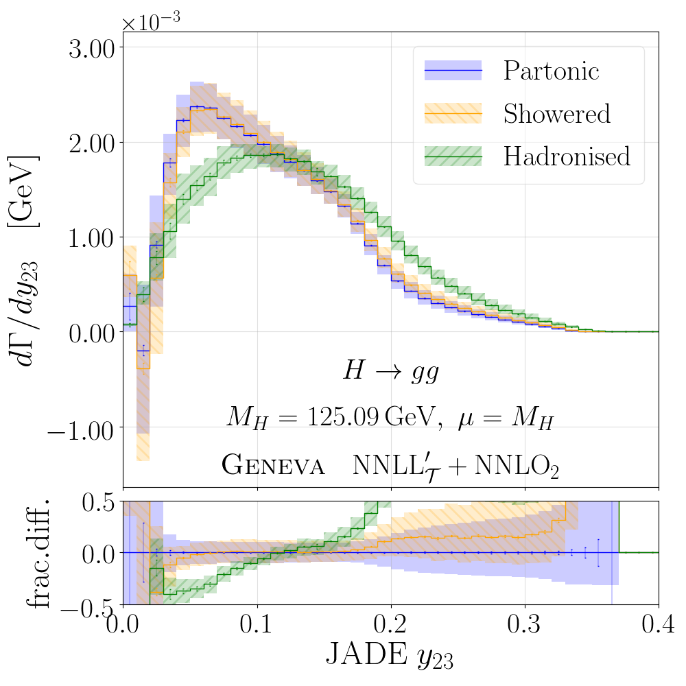
Figure 9: Jet broadening and the JADE two-to-three differential jet rate at the partonic, showered and hadronised levels for $H\to b\bar{b}$.

Figure 10: Jet broadening and the JADE two-to-three differential jet rate at the partonic, showered and hadronised levels for $H\to gg$.

Finally, in figs. 10 and 10 we show the results for distributions other than the $2$-jettiness that we use as input to our Geneva implementation, for the $b\bar{b}$ and $gg$ cases respectively. We consider the JADE clustering metric $y_{23}$ for separating two exclusive jets from three or more Bartel:1982ub ; Bartel:1986ua and the jet broadening ($B_{T}$) Rakow:1981qn ; Catani:1992jc event shape defined as follows

$$B_{T} =\frac{1}{2\sum_{k}\lvert\vec{p}_{k}\rvert}\sum_{i}\lvert\vec{p}_{i}\times\hat{n}_{T}\rvert\,,$$ (32)

where the sum runs over all final state particles and $\hat{n}_{T}$ is the thrust axis.

It is important to remark that we do not expect the Geneva method to provide a higher formal accuracy for these observables, but it is nonetheless interesting to observe the effects of our predictions at the various stages. In general the $b\bar{b}$ decay channel is better behaved after showering, providing results that are compatible with the predictions at the partonic level over the majority of the phase space.

We notice that, at small values of the jet broadening, some unappealing artefacts appear. We have verified that these features are a consequence of the additive matching to the fixed-order calculation, used to include the nonsingular corrections. They are not present, for example, when examining the jet broadening distribution of events obtained from the $\mathcal{T}_{2}$ resummed calculation alone. We therefore conclude that the secondary peak which appears constitutes an effect beyond the perturbative accuracy of our formulae, despite being numerically large. In the future, one could explore whether by exploiting the freedom in the handling of the recoil by the $3\to 4$ mapping one could ameliorate this undesirable effect – however, we do not pursue this further here. We also see deviations for particular values of the observables after hadronisation and hadron decays are included. In particular we notice a significant shift in the JADE $y_{23}$ observable for both decay channels, which is not unexpected for this specific jet-clustering measure.

5 Conclusions

In this work we have resummed the $2$-jettiness at NNLL^′ for hadronic Higgs boson decays in the $b\bar{b}$ and $gg$ channels via a SCET approach. Compared to previous fixed-order results, we observe the expected improved behaviour in the small $\mathcal{T}_{2}$ region, where the physical Sudakov peak is now described correctly. We have also implemented these processes in the Geneva framework, which has allowed us to match the resummed calculations with NNLO fixed-order predictions and to a parton shower. This has required an examination of the interplay of the singular and nonsingular contributions, in order to determine the region in which resummation effects are dominant and hence design profile scales which provide a smooth transition between the resummed and fixed-order regimes. As a result we have produced NNLO accurate event generators interfaced to the Pythia8 parton shower for the two processes, which provide accurate predictions in all regions of phase space.

We compared predictions at the partonic, showered and hadronised levels, finding the expected good agreement for the total decay rates and for the $\mathcal{T}_{2}$ distribution up to the showered level. We observed larger differences due to the hadronisation, especially in the $gg$ channel.

The completion of this work will eventually allow us to combine our $H\rightarrow b\bar{b}$ result with the Geneva $VH$ production generator in the narrow width approximation, yielding a full NNLOPS generator for the signal channel of the $l^{+}l^{-}b\bar{b}$ final state. Given the recent observation of the Higgsstrahlung process by the ATLAS & CMS experiments at the LHC Sirunyan:2018kst ; Aaboud:2018zhk , this will constitute an important phenomenological result. It will also allow a direct comparison with the only other existing NNLOPS generator for this process Bizon:2019tfo . In light of the findings in Ref. Gao:2019mlt regarding the convergence of the perturbative series and the N³LO results at fixed order which are also available for this decay channel, it might also be interesting to consider building an event generator at N³LOPS level. Another avenue for development might be the inclusion of a finite $b$-quark mass in the generator, given recent work on fixed-order calculations Behring:2020uzq . We leave this to future consideration.

Appendix A Constructing a $2$-jettiness-preserving map

The map used for $3\to 4$-body splittings and $4\to 3$-body projections presented in this section was first developed and applied to the process $e^{+}e^{-}\rightarrow jj$ in Ref. Alioli:2012fc . Here, we detail the construction of the map as used in that work and in addition provide the translation to the splitting variables $\mathcal{T}_{2},\,z$ and $\phi$ needed for the Higgs boson decay case.

We start by considering the case of a splitting, which takes as input $N$-body phase space points $\Phi_{N}$ and generates from them $(N\!+\!1)$-body phase-space points $\Phi_{N+1}$. Since we wish to calculate the NLO distribution in $2$-jettiness, $\mathcal{T}_{2}$, while still generating exclusive $\Phi_{3}$ points, we must use a map that produces $\Phi_{4}$ points with the same value of $\mathcal{T}_{2}$ as the $\Phi_{3}$ points with which we started. Unfortunately, the construction of such a map is challenging since $\mathcal{T}_{2}$ is a global variable. A more manageable approach is to seek a map which preserves not the exact $2$-jettiness, $\mathcal{T}_{2}$, but instead a related quantity, the fully recursive $2$-jettiness, $\mathcal{T}_{2}^{\mathrm{FR}}$, defined by the following procedure:

1. Recursively cluster the starting phase space point $\Phi_{M}$ down to a $\Phi_{3}$ point using the $N$-jettiness metric for final state particles

   $$\rho_{ij}=|\vec{p}_{i}|+|\vec{p}_{j}|-|\vec{p}_{i}+\vec{p}_{j}|.$$ (33)

2. Measure $\mathcal{T}_{2}$ on the resulting $\Phi_{3}$ point.

The quantity we obtain through this procedure has the same singular structure as the exact $\mathcal{T}_{2}$, with any differences being captured by the nonsingular contributions.

Starting from the $3$-parton phase space point $\Phi_{3}$, which is the input of the splitting map, we label its momenta as

$$p_{1},\,p_{2},\,p_{3}\quad\mathrm{with}\quad p_{1}^{0}>p_{2}^{0}>p_{3}^{0}\,.$$ (34)

The thrust axis will lie along the direction of the hardest parton (i.e. along $\vec{p}_{1}$), and we have that

$$\mathcal{T}_{2}^{\mathrm{FR}}=\mathcal{T}_{2}=2E_{\mathrm{cm}}-4|\vec{p}_{1}|\,.$$ (35)

When we split to a $4$-parton event and then cluster back to a massive $3$-parton event, the thrust axis is still determined by the most energetic of the three partons and we have that

$$\mathcal{T}_{2}^{\mathrm{FR}}=2E_{\mathrm{cm}}-4|\vec{p}_{\mathrm{max}}|\,.$$ (36)

If we are to preserve $\mathcal{T}_{2}^{\mathrm{FR}}$, clearly eqs. (35) and (36) must be equal and so the hardest parton in the massive $3$-parton event obtained after reclustering must be parton 1. We can then split the massive leg to produce a $4$-parton point. The emitter may or may not be the hardest parton – these two cases must be treated separately.

We will now detail how the $\Phi_{4}$ point is obtained from the $\Phi_{3}$ point in the two separate cases while preserving $\mathcal{T}_{2}^{\mathrm{FR}}$. In addition, we will show in each case that taking the singular limits of the Jacobian of the transformation reproduces the limits of the FKS Jacobian and that our fixed-order subtractions in eq. (14) therefore survive unaltered.

A.1 Case 1: the emitter as hardest parton

We deal first with the case in which the emitter is the hardest parton, which we call the FR primary (FRp) map. In this case the emitter is $p_{1}$ and, denoting the sum of the momenta of the split pair by $k$, we must have that $\vec{k}\parallel\vec{p}_{1}$ in order to keep the thrust axis in the same direction. We must also have $|\vec{k}|=|\vec{p}_{1}|$. These conditions therefore fix the sum of the three-momenta of the split pair.

In order to proceed with the actual construction of the split configuration we use the same choice of variables as in the FKS approach, and therefore adopt a similar notation: we label the momenta in $\Phi_{3}$ by $\bar{k}_{1},\bar{k}_{2},\bar{k}_{3}$, with the emitter chosen as $\bar{k}_{3}$. For the $\Phi_{4}$ momenta we use $k_{1},\dots,k_{4}$ with the split pair $k_{3},k_{4}$ and $k=k_{3}+k_{4}$. The recoil momenta are defined as

$$\bar{k}_{\mathrm{rec}} =\bar{k}_{1}+\bar{k}_{2}\,, k_{\mathrm{rec}} =k_{1}+k_{2}\,.$$ (37)

As discussed above, the splitting preserves the three-momentum of the emitter which constrains the momentum of the split pair and the recoil:

$$\bar{k}_{3} =(\bar{k}_{3}^{0},\vec{\bar{k}}_{3}), \bar{k}_{\mathrm{rec}} =(\bar{k}^{0}_{\mathrm{rec}},-\vec{\bar{k}}_{3})=(E_{\mathrm{cm}}-\bar{k}^{0}_{3},-\vec{\bar{k}}_{3})\,,$$ (38)

$$k =(k^{0},\vec{\bar{k}}_{3}), k_{\mathrm{rec}} =(k^{0}_{\mathrm{rec}},-\vec{\bar{k}}_{3})=(E_{\mathrm{cm}}-k^{0},-\vec{\bar{k}}_{3})\,.$$ (39)

We must now determine $k^{0}$ and define the recoil constituents such that they remain massless and sum to $k_{\mathrm{rec}}$. Since we have that $|\vec{k}|=|\vec{\bar{k}}_{3}|=\bar{k}_{3}^{0}$, we may obtain an expression for $k^{0}$:

$$k^{2}=(k^{0})^{2}-|\vec{k}|^{2}=(k^{0})^{2}-(\bar{k}^{0}_{3})^{2}\,.$$ (40)

Recalling the definitions of the FKS variables $\Phi_{\mathrm{rad}}^{\mathrm{FKS}}\equiv\{\xi,y,\phi\}$

$$k_{4}^{0} =\frac{1}{2}E_{\mathrm{cm}}\xi, k^{2}=2k_{3}^{0}k_{4}^{0}(1-y)\,,$$ (41)

we may substitute in and solve the quadratic equation; one obtains

$$k^{0} =\frac{1}{2}E_{\mathrm{cm}}\xi(1-y)\pm\left((\bar{k}^{0}_{3})^{2}-\left(\frac{1}{2}E_{\mathrm{cm}}\xi\right)^{2}(1-y^{2})\right)^{1/2}\,,$$ (42)

$$k^{0}_{3} =-\frac{1}{2}E_{\mathrm{cm}}\xi y\pm\left((\bar{k}^{0}_{3})^{2}-\left(\frac{1}{2}E_{\mathrm{cm}}\xi\right)^{2}(1-y^{2})\right)^{1/2}\,.$$ (43)

Having determined $k^{0}$ in terms of $\xi$ and $y$, we must carefully examine which solutions are kinematically allowed. The specific $\Phi_{\mathrm{rad}}^{\mathrm{FKS}}$ variables determine which (if either) of these roots are permitted. In addition to ensuring that the solutions are real, we must also have that $k^{0}>\bar{k}^{0}_{3}$ and that $k_{3}^{0}>0$. The reality constraint gives

$$\bar{k}^{0}_{3}>\frac{1}{2}E_{\mathrm{cm}}\xi\sqrt{1-y^{2}}\qquad\Rightarrow\qquad\xi<\frac{2\bar{k}^{0}_{3}}{E_{\mathrm{cm}}}\frac{1}{\sqrt{1-y^{2}}}\,.$$ (44)

The effect of the remaining two constraints is determined by the sign of $y$. For $y>0$, only the positive root is a valid solution (since $k_{3}^{0}<0$ for the negative root), and we have a stronger constraint on $\xi$:

$$y>0:\mbox{positive root for }\xi<\frac{2\bar{k}^{0}_{3}}{E_{\mathrm{cm}}}\,.$$ (45)

For $y<0$, the positive root is valid over the range in $\xi$ set by the real constraint, and the negative root is valid for $\xi>2\bar{k}^{0}_{3}/E_{\mathrm{cm}}$:

$$y<0:\, \mbox{positive root for }\xi<\frac{2\bar{k}^{0}_{3}}{E_{\mathrm{cm}}}\frac{1}{\sqrt{1-y^{2}}}$$ (46)

$$\mbox{negative root for }\frac{2\bar{k}^{0}_{3}}{E_{\mathrm{cm}}}<\xi<\frac{2\bar{k}^{0}_{3}}{E_{\mathrm{cm}}}\frac{1}{\sqrt{1-y^{2}}}\,.$$ (47)

It remains for us to construct the four momenta of the $\Phi_{4}$ event. We define

$$\delta=\frac{k^{0}}{\bar{k}^{0}_{3}}-1\,,$$ (48)

and the parameter

$$\beta_{\mathrm{rec}}=\frac{|\vec{\bar{k}}_{\mathrm{rec}}|}{\bar{k}^{0}_{\mathrm{rec}}}=\frac{\bar{k}^{0}_{3}}{E_{\mathrm{cm}}-\bar{k}^{0}_{3}}\,.$$ (49)

We assign the recoil by defining a boost $\mathcal{B}_{t}$ along $\vec{\bar{k}}_{\mathrm{rec}}$ with magnitude $\beta_{t}$ and a constant scaling of momenta $\alpha$, so that

$$k_{i} =\alpha(\mathcal{B}_{t}\bar{k}_{i})\,, i =1,2\,.$$ (50)

Boosting along the recoil direction and then rescaling momenta allows us to keep the recoil three-momentum fixed. We can solve for the parameters $\alpha$ and $\beta_{t}$ using

$$k_{\mathrm{rec}}=\alpha(\mathcal{B}_{t}\bar{k}_{\mathrm{rec}})\,,$$ (51)

which gives two constraints:

$$k^{0}_{\mathrm{rec}} =\alpha\gamma_{t}\bar{k}^{0}_{\mathrm{rec}}(1+\beta_{t}\beta_{\mathrm{rec}})\,,$$ (52)

$$|\vec{k}_{\mathrm{rec}}| =\alpha\gamma_{t}\bar{k}^{0}_{\mathrm{rec}}(\beta_{t}+\beta_{\mathrm{rec}})\,.$$ (53)

These can be solved in terms of $\delta$ and $\bar{k}^{0}_{3}$ to obtain

$$\beta_{t} =\frac{\beta_{\mathrm{rec}}^{2}\delta}{1-\beta_{\mathrm{rec}}^{2}-\beta_{\mathrm{rec}}\delta}\,, \alpha =\sqrt{1-\beta_{t}^{2}}\left(1+\frac{\beta_{t}}{\beta_{\mathrm{rec}}}\right)^{-1}\,.$$ (54)

For the splitting to exist, we must also ensure that $0<\beta_{t}<1$. Rewriting $\beta_{t}$ as

$$\beta_{t} =\frac{\bar{k}_{3}^{0}(k^{0}-\bar{k}_{3}^{0})}{\bar{k}^{0}_{3}(k^{0}-\bar{k}^{0}_{3})+E_{\mathrm{cm}}(k^{0}_{\mathrm{rec}}-\bar{k}^{0}_{3})}$$ (55)

$$=1-\frac{E_{\mathrm{cm}}(k^{0}_{\mathrm{rec}}-\bar{k}^{0}_{3})}{\bar{k}^{0}_{3}(k^{0}-\bar{k}^{0}_{3})+E_{\mathrm{cm}}(k^{0}_{\mathrm{rec}}-\bar{k}^{0}_{3})}\,,$$ (56)

we see that for $k^{0},k^{0}_{\mathrm{rec}}>\bar{k}^{0}_{3}$ (i.e. for timelike $k,k_{\mathrm{rec}}$), the condition on $\beta_{t}$ is satisfied. Specifically, we require

$$\bar{k}^{0}_{3}<k^{0}<E_{\mathrm{cm}}-\bar{k}^{0}_{3}\,.$$ (57)

The upper bound on $k^{0}$ implies the additional constraint

$$x<1-\frac{2\bar{k}_{3}^{0}}{E_{\mathrm{cm}}}$$ (58)

where $x=k^{2}/E_{\mathrm{cm}}^{2}$. This can be translated into a constraint on $\xi$ and $y$. We may then split $k$ into $k_{3}$ and $k_{4}$ using the FKS variables in the same way as for the FKS splitting.

We can also invert the procedure and construct the projective map from $\Phi_{4}$ to $\Phi_{3}$. Again we must preserve the three-momentum of the split pair, so that

$$\Phi_{4}:\ k=(k^{0},\vec{k})\,, k_{\mathrm{rec}}=(E_{\mathrm{cm}}-k^{0},-\vec{k})\,,$$ (59)

$$\Phi_{3}:\ \bar{k}_{3}=(|\vec{k}|,\vec{k})\,, \bar{k}_{\mathrm{rec}}=(E_{\mathrm{cm}}-|\vec{k}|,-\vec{k})\,.$$ (60)

We need only now define the individual partons in the recoil, which we achieve by using the same boost technique as before. Defining

$$\bar{k}_{i}=\mathcal{B}_{t}^{-1}\left(\frac{1}{\alpha}k_{i}\right)$$ (61)

where the inverse boost is now along $-\vec{k}_{\mathrm{rec}}$, as before we can obtain two constraints:

$$E_{\mathrm{cm}}-|\vec{k}| =\frac{\gamma_{t}}{\alpha}(k^{0}_{\mathrm{rec}}-\beta_{t}|\vec{k}|)\,,$$ (62)

$$|\vec{k}| =\frac{\gamma_{t}}{\alpha}(|\vec{k}|-\beta_{t}k^{0}_{\mathrm{rec}})\,.$$ (63)

Solving, we naturally recover the same $\alpha$ and $\beta_{t}$ as in eq. (54). In this case, however, the constraints $0<\beta_{t}<1$ and $0<\alpha<1$ are automatically satisfied so that the projection from any $\Phi_{4}$ point onto a $\Phi_{3}$ point is well-defined.

Finally, we must show that the limits of the splitting Jacobian are indeed equivalent to those in the FKS case. After manipulation of the above expressions, we find that

$$\mathrm{d}\Phi_{4}(q;k1,\dots,k_{4})=J_{\mathrm{FRp}}\mathrm{d}\Phi_{3}(q;\bar{k}_{1},\dots,\bar{k}_{3})\mathrm{d}\Phi_{\mathrm{rad}}^{\mathrm{FKS}}(\xi,y,\phi)\,,$$ (64)

where

$$\mathrm{d}\Phi^{\mathrm{FKS}}_{\mathrm{rad}}=\frac{1}{(4\pi)^{3}}\mathrm{d}\xi\mathrm{d}y\mathrm{d}\phi$$ (65)

and

$$J_{\mathrm{FRp}}=E_{\mathrm{cm}}^{2}\xi\left(\frac{2k^{0}-E_{\mathrm{cm}}\xi}{2k^{0}+E_{\mathrm{cm}}\xi(y-1)}\right)\,.$$ (66)

Substituting eq. (42) into eq. (66), one can verify that taking the limit $\alpha\rightarrow 1$ and expanding about $\xi=0$ or $y=1$ one obtains the soft or collinear limits of the FKS Jacobian, see e.g. section 5 of Frixione:2007vw . This means that one can use the same counterterms as those of the FKS subtraction to obtain a local cancellation of the infrared divergences.

A.2 Case 2: the emitter as a softer parton

In the case where the emitter is not the most energetic particle, the FRp map is no longer appropriate because we no longer need to keep the thrust-axis aligned with the emitter. In this case, we can use instead the Catani-Seymour (CS) map Catani:1996jh . For example, if we assume the emitter is $p_{2}$ and perform the splitting considering $p_{3}$ as the spectator parton, the hardest parton $p_{1}$ is then unchanged by the splitting and the quantity $(p_{2}+p_{3})^{2}$ is preserved. This means that the thrust axis remains along $\vec{p}_{1}$ and that the value of $\mathcal{T}_{2}^{\mathrm{FR}}$ is also unchanged. It is left for us to show that the singular limit of the Jacobian when using the CS map with FKS variables is the same as in the FKS case up to an overall rescaling.

To describe the splitting in this case we adopt the CS notation, where $\tilde{p}_{ij}$ is the emitter and $\tilde{p}_{k}$ is the recoil in the $\Phi_{3}$ phase space. The daughters of the splitting are labelled $p_{i}$ and $p_{j}$, while $p_{k}$ is the recoil in the $\Phi_{4}$ phase space:

$$\tilde{p}_{ij}+\tilde{p_{k}}\rightarrow p_{i}+p_{j}+p_{k}=p_{ij}+p_{k}.$$ (67)

For the case at hand, we begin by factorising $\Phi_{4}$ into the $4$-parton CS phase space and a radiation part

$$\mathrm{d}\Phi_{4}=\mathrm{d}\Phi_{3}^{\mathrm{CS}}(1-y_{ij,k})E_{\mathrm{cm}}^{2}\mathrm{d}\Phi_{\mathrm{rad}}(x,\Omega_{2})$$ (68)

where

$$y_{ij,k}=\frac{p_{i}\cdot p_{j}}{p_{i}\cdot p_{j}+p_{i}\cdot p_{k}+p_{j}\cdot p_{k}}=\frac{(p_{i}+p_{j})^{2}}{(p_{i}+p_{j}+p_{k})^{2}}$$ (69)

and $x,\Omega_{2}$ are a set of variables which parameterise the splitting $p_{ij}\rightarrow p_{i}+p_{j}$. We now wish to express the $\{x,\cos\theta\}$ in terms of the FKS variables $\{\xi,y\}$ which we do using the defining relations of the CS and FKS variables:

$$p_{ij} =\tilde{p}_{ij}+\frac{p_{ij}^{2}}{2\tilde{p}_{ij}\cdot\tilde{p}_{k}}\tilde{p}_{k},$$ (70)

$$p_{ij}^{2} =xE_{\mathrm{cm}}^{2}=2p_{i}^{0}p_{j}^{0}(1-y),$$ (71)

$$p_{i}^{0} =\frac{1}{2}E_{\mathrm{cm}}\xi,$$ (72)

$$\xi =\frac{1}{E_{\mathrm{cm}}}(p_{ij}^{0}+|\vec{p}_{ij}|\cos\theta).$$ (73)

Solving, we find that

$$E_{\mathrm{cm}}\xi =\left(\tilde{p}^{0}_{ij}+\frac{xE_{\mathrm{cm}}^{2}}{2\tilde{p}_{ij}\cdot\tilde{p}_{k}}\tilde{p}^{0}_{k}\right)+\sqrt{\left(\tilde{p}^{0}_{ij}+\frac{xE_{\mathrm{cm}}^{2}}{2\tilde{p}_{ij}\cdot\tilde{p}_{k}}\tilde{p}^{0}_{k}\right)^{2}-xE_{\mathrm{cm}}^{2}}\cos\theta,$$ (74)

$$y =1-xE_{\mathrm{cm}}^{2}\left[E_{\mathrm{cm}}\xi\left(\tilde{p}^{0}_{ij}+\frac{xE_{\mathrm{cm}}^{2}}{2\tilde{p}_{ij}\cdot\tilde{p}_{k}}\tilde{p}^{0}_{k}-\frac{1}{2}E_{\mathrm{cm}}\xi\right)\right]^{-1}.$$ (75)

The Jacobian of this transformation is given by

$$\frac{\mathrm{d}x\,\mathrm{d}\cos\theta}{\mathrm{d}\xi\mathrm{d}y}\equiv J(x,\cos\theta;\xi,y)=\xi\left(\frac{2p^{0}_{ij}}{E_{\mathrm{cm}}}-\xi\right)^{2}\left(\frac{2\tilde{p}^{0}_{ij}}{E_{\mathrm{cm}}}-\xi\right)^{-1}\left(\frac{2|\vec{p}_{ij}|}{E_{\mathrm{cm}}}\right)^{-1}$$ (76)

so that we have

$$\mathrm{d}\Phi_{4} =\mathrm{d}\Phi_{3}^{\mathrm{CS}}(1-y_{ij,k})\frac{2\tilde{p}_{ij}\cdot\tilde{p}_{k}}{(4\pi)^{2}2\pi}J(x,\cos\theta;\xi,y)\mathrm{d}\xi\mathrm{d}y\mathrm{d}\phi$$ (77)

$$\equiv\mathrm{d}\Phi^{\mathrm{CS}}_{N}J^{\mathrm{CS}}_{\mathrm{FKS}}(\xi,y)\mathrm{d}\Phi^{\mathrm{FKS}}_{\mathrm{rad}},$$ (78)

and the total Jacobian is

$$J^{\mathrm{CS}}_{\mathrm{FKS}}(\xi,y)=\left(1-\frac{p_{ij}^{2}}{2\tilde{p}_{ij}\cdot\tilde{p}_{k}}\right)E_{\mathrm{cm}}^{2}\xi\left(\frac{2p_{ij}^{0}}{E_{\mathrm{cm}}}-\xi\right)^{2}\left(\frac{2\tilde{p}^{0}_{ij}}{E_{\mathrm{cm}}}-\xi\right)^{-1}\left(\frac{2|\vec{p}_{ij}|}{E_{\mathrm{cm}}}\right)^{-1}.$$ (79)

The soft and collinear limits of this expression are

$$J^{\mathrm{CS}}_{\mathrm{FKS}}(\xi\rightarrow 0,y) =E_{\mathrm{cm}}^{2}\xi,$$ (80)

$$J^{\mathrm{CS}}_{\mathrm{FKS}}(\xi,y\rightarrow 1) =E_{\mathrm{cm}}^{2}\xi\left(1-\frac{\xi}{\xi_{\mathrm{max}}}\right),$$ (81)

which are exactly the soft and collinear limits of the Jacobian in the usual FKS map. Once again, the consequence is that the subtractions are precisely the same as in the FKS case and we are therefore able to use the CS mapping consistently with the FKS subtractions.

A.3 Recasting the mapping for use in the splitting functions

The mapping which we have constructed in this appendix is used not only in the fixed-order pieces of eqs. (3.1) and (3.1) but also to make the resummed spectrum fully differential in $\Phi_{4}$ via the splitting function defined in eq. (18). We must therefore be able to construct a $\Phi_{4}$ phase space point using the mapping given a $\Phi_{3}$ point and values of three splitting variables. This can be achieved à la FKS, but in order to do so we must express our splitting variables in eq. (18) in terms of the FKS variables.

We consider four momenta $p^{\prime}_{12},\,p^{\prime}_{3},\,p^{\prime}_{4}$ before the splitting producing a configuration $p_{1},\,p_{2},\,p_{3},\,p_{4}$ afterwards and assume the hierarchy $E_{1}<E_{2}<E_{3}<E_{4}$. Our splitting variables are defined to be the azimuthal angle $\phi$, the $3$-jettiness $\mathcal{T}_{3}$ and an energy ratio $z$:

$$\mathcal{T}_{3} =2\left(E_{1}+E_{2}-\lvert\vec{p}_{12}\rvert\right),$$ (82)

$$z =\frac{E_{1}}{E_{1}+E_{2}},$$ (83)

where $\lvert\vec{p}_{12}\rvert=\lvert\vec{p}_{1}+\vec{p}_{2}\rvert$. Rewriting, we have that

$$E_{1} =z\left(\frac{1}{2}\mathcal{T}_{3}+\lvert\vec{p}_{12}\rvert\right),$$

$$E_{2} =(1-z)\left(\frac{1}{2}\mathcal{T}_{3}+\lvert\vec{p}_{12}\rvert\right),$$

$$E_{34} =M_{H}-\frac{1}{2}\mathcal{T}_{3}-\lvert\vec{p}_{12}\rvert,$$ (84)

while the energy hierarchy which we have assumed limits $z$ to the range

$$2-\frac{M_{H}}{\frac{1}{2}\mathcal{T}_{3}+\lvert\vec{p}_{12}\rvert}<z<\frac{1}{2}.$$ (85)

From the definitions of the FKS variables, we have that

$$\xi =\frac{2z}{M_{H}}\left(\frac{1}{2}\mathcal{T}_{3}+\lvert\vec{p}_{12}\rvert\right),$$ (86)

$$y =1-\frac{\mathcal{T}_{3}^{2}+4\mathcal{T}_{3}\lvert\vec{p}_{12}\rvert}{8z(1-z)\left(\frac{1}{2}\mathcal{T}_{3}+\lvert\vec{p}_{12}\rvert\right)^{2}},$$ (87)

and the Jacobian of the transformation is given by

$$J_{\mathrm{split}}=\Biggr{\lvert}\frac{(1+2\lvert\vec{p}_{12}\rvert)\left[\frac{1}{2}z\mathcal{T}_{3}-(1-z)\lvert\vec{p}_{12}\rvert\right]+\mathcal{T}_{3}\left[1-\mathcal{T}_{3}(1-z)+2z\lvert\vec{p}_{12}\rvert\right]\frac{\partial\lvert\vec{p}_{12}\rvert}{\partial\mathcal{T}_{3}}}{M_{H}z(1-z)^{2}\left(\frac{1}{2}\mathcal{T}_{3}+\lvert\vec{p}_{12}\rvert\right)^{2}}\Biggr{\rvert}.$$ (88)

It remains for us to determine the quantity $\lvert\vec{p}_{12}\rvert$ in terms of the $\Phi_{3}$ momenta. This depends on whether the FRp or CS map is being used. In the FRp case, this is rather straightforward – the FRp map preserves the value of $\lvert\vec{p}_{12}\rvert$ by construction and so we have that $\lvert\vec{p}_{12}\rvert=\lvert\vec{p}\,^{\prime}_{12}\rvert$. Thus, the last term in the numerator of eq. (88) disappears and the expression simplifies. In the CS case, matters are slightly more complicated. The map preserves the four-momentum of the most energetic particle $p_{4}^{\prime}$ while $p_{3}^{\prime}$ is the spectator; from the definition of the CS variables, we have that

$$p_{4} =p_{4}^{\prime},$$

$$p_{3} =(1-y_{12,3})p_{3}^{\prime}.$$ (89)

Using the definition of $y_{ij,k}$ in eq. (69), we find that

$$\lvert\vec{p}_{12}\rvert=\frac{\frac{1}{2}\mathcal{T}_{3}-M_{H}+E^{\prime}_{4}+\left(1-\frac{\mathcal{T}_{3}^{2}}{4(p^{\prime}_{12}+p^{\prime}_{3})^{2}}\right)E^{\prime}_{3}}{\frac{E^{\prime}_{3}\mathcal{T}_{3}}{(p^{\prime}_{12}+p^{\prime}_{3})^{2}}-1},$$ (90)

where the right hand side is expressed solely in terms of primed quantities and splitting variables. We may then substitute into eq. (88) which provides us with all the information we require.

Appendix B NNLO decay rates

For convenience, we list here the NNLO decay rates of the Higgs boson to $b$-quarks and to gluons, taken from Chetyrkin:1996sr ; Schreck:2007um . In the following, $L_{H}\equiv\log(\mu^{2}/M_{H}^{2})$ and $L_{t}\equiv\log(\mu^{2}/m_{t}^{2})$, we have set $N_{c}=3$ and $n_{\ell}$ is the number of light active flavours.

$$\Gamma^{b}_{\mathrm{NNLO}}(\mu)=\Gamma_{\mathrm{B}}^{b}(\mu)\Bigg{\{}1 +\left(\frac{\alpha_{\rm s}(\mu)}{4\pi}\right)\left[\frac{68}{3}+8L_{H}\right]$$

$$+\left(\frac{\alpha_{\rm s}(\mu)}{4\pi}\right)^{2}\bigg{[}\frac{10801}{9}-\frac{76\pi^{2}}{3}-312\zeta(3)+\frac{1696}{3}L_{H}+76L_{H}^{2}$$

$$+n_{\ell}\left(-\frac{130}{3}+\frac{8\pi^{2}}{9}+\frac{32}{3}\zeta(3)-\frac{176}{9}L_{H}-\frac{8}{3}L_{H}^{2}\right)\bigg{]}\Bigg{\}}$$ (91)

$$\Gamma^{g}_{\mathrm{NNLO}}(\mu)=\Gamma_{\mathrm{B}}^{g}(\mu)\Bigg{\{}1 +\left(\frac{\alpha_{\rm s}(\mu)}{4\pi}\right)\bigg{[}95+22L_{H}+n_{\ell}\left(-\frac{14}{3}-\frac{4}{3}L_{H}\right)\bigg{]}$$

$$+\left(\frac{\alpha_{\rm s}(\mu)}{4\pi}\right)^{2}\bigg{[}\frac{149533}{18}-121\pi^{2}-990\zeta(3)+3301L_{H}+363L_{H}^{2}+38L_{t}$$

$$+n_{\ell}\left(-\frac{8314}{9}+\frac{44\pi^{2}}{3}+20\zeta(3)-380L_{H}-44L_{H}^{2}+\frac{32}{3}L_{t}\right)$$

$$+n_{\ell}^{2}\left(\frac{508}{27}-\frac{4\pi^{2}}{9}+\frac{28}{3}L_{H}+\frac{4}{3}L_{H}^{2}\right)\bigg{]}\Bigg{\}}$$ (92)

References

- (1) J. Davies, M. Steinhauser and D. Wellmann, Completing the hadronic Higgs boson decay at order , Nucl. Phys. B 920 (2017) 20–31, [1703.02988].
- (2) LHC Higgs Cross Section Working Group collaboration, D. de Florian et al., Handbook of LHC Higgs Cross Sections: 4. Deciphering the Nature of the Higgs Sector, 1610.07922.
- (3) CMS collaboration, A. M. Sirunyan et al., Observation of Higgs boson decay to bottom quarks, Phys. Rev. Lett. 121 (2018) 121801, [1808.08242].
- (4) ATLAS collaboration, M. Aaboud et al., Observation of decays and production with the ATLAS detector, Phys. Lett. B 786 (2018) 59–86, [1808.08238].
- (5) P. Baikov, K. Chetyrkin and J. H. Kühn, Scalar correlator at , Higgs decay into b-quarks and bounds on the light quark masses, Phys. Rev. Lett. 96 (2006) 012003, [hep-ph/0511063].
- (6) S. Gorishnii, A. Kataev and S. Larin, The Width of Higgs Boson Decay Into Hadrons: Three Loop Corrections of Strong Interactions, Sov. J. Nucl. Phys. 40 (1984) 329–334.
- (7) S. Gorishnii, A. Kataev, S. Larin and L. Surguladze, Corrected Three Loop QCD Correction to the Correlator of the Quark Scalar Currents and ( Hadrons), Mod. Phys. Lett. A 5 (1990) 2703–2712.
- (8) S. Gorishnii, A. Kataev, S. Larin and L. Surguladze, Scheme dependence of the next to next-to-leading QCD corrections to ( hadrons) and the spurious QCD infrared fixed point, Phys. Rev. D 43 (1991) 1633–1640.
- (9) C. Becchi, S. Narison, E. de Rafael and F. Yndurain, Light Quark Masses in Quantum Chromodynamics and Chiral Symmetry Breaking, Z. Phys. C 8 (1981) 335.
- (10) N. Sakai, Perturbative QCD Corrections to the Hadronic Decay Width of the Higgs Boson, Phys. Rev. D 22 (1980) 2220.
- (11) K. Chetyrkin, Correlator of the quark scalar currents and ( hadrons) at in pQCD, Phys. Lett. B 390 (1997) 309–317, [hep-ph/9608318].
- (12) K. Chetyrkin and M. Steinhauser, Complete QCD corrections of order to the hadronic Higgs decay, Phys. Lett. B 408 (1997) 320–324, [hep-ph/9706462].
- (13) C. Anastasiou, F. Herzog and A. Lazopoulos, The fully differential decay rate of a Higgs boson to bottom-quarks at NNLO in QCD, JHEP 03 (2012) 035, [1110.2368].
- (14) V. Del Duca, C. Duhr, G. Somogyi, F. Tramontano and Z. Trócsányi, Higgs boson decay into b-quarks at NNLO accuracy, JHEP 04 (2015) 036, [1501.07226].
- (15) R. Mondini, M. Schiavi and C. Williams, N3LO predictions for the decay of the Higgs boson to bottom quarks, JHEP 06 (2019) 079, [1904.08960].
- (16) R. Mondini, U. Schubert and C. Williams, Top-induced contributions to and at , 2006.03563.
- (17) A. Primo, G. Sasso, G. Somogyi and F. Tramontano, Exact Top Yukawa corrections to Higgs boson decay into bottom quarks, Phys. Rev. D 99 (2019) 054013, [1812.07811].
- (18) W. Bernreuther, L. Chen and Z.-G. Si, Differential decay rates of CP-even and CP-odd Higgs bosons to top and bottom quarks at NNLO QCD, JHEP 07 (2018) 159, [1805.06658].
- (19) A. Behring, W. Bizoń, F. Caola, K. Melnikov and R. Röntsch, Bottom quark mass effects in associated production with the decay through NNLO QCD, Phys. Rev. D 101 (2020) 114012, [2003.08321].
- (20) K. Chetyrkin, B. A. Kniehl and M. Steinhauser, Hadronic Higgs decay to order , Phys. Rev. Lett. 79 (1997) 353–356, [hep-ph/9705240].
- (21) F. Caola, K. Melnikov and R. Röntsch, Analytic results for decays of color singlets to and final states at NNLO QCD with the nested soft-collinear subtraction scheme, Eur. Phys. J. C 79 (2019) 1013, [1907.05398].
- (22) P. Baikov and K. Chetyrkin, Top Quark Mediated Higgs Boson Decay into Hadrons to Order , Phys. Rev. Lett. 97 (2006) 061803, [hep-ph/0604194].
- (23) F. Herzog, B. Ruijl, T. Ueda, J. Vermaseren and A. Vogt, On Higgs decays to hadrons and the R-ratio at N4LO, JHEP 08 (2017) 113, [1707.01044].
- (24) M. Schreck and M. Steinhauser, Higgs Decay to Gluons at NNLO, Phys. Lett. B 655 (2007) 148–155, [0708.0916].
- (25) M. Spira, Higgs Boson Production and Decay at Hadron Colliders, Prog. Part. Nucl. Phys. 95 (2017) 98–159, [1612.07651].
- (26) J. Gao, Y. Gong, W.-L. Ju and L. L. Yang, Thrust distribution in Higgs decays at the next-to-leading order and beyond, JHEP 03 (2019) 030, [1901.02253].
- (27) S. Alioli, C. W. Bauer, C. Berggren, A. Hornig, F. J. Tackmann et al., Combining Higher-Order Resummation with Multiple NLO Calculations and Parton Showers in GENEVA, JHEP 1309 (2013) 120, [1211.7049].
- (28) S. Alioli, C. W. Bauer, C. Berggren, F. J. Tackmann, J. R. Walsh et al., Matching Fully Differential NNLO Calculations and Parton Showers, JHEP 1406 (2014) 089, [1311.0286].
- (29) S. Alioli, C. W. Bauer, C. Berggren, F. J. Tackmann and J. R. Walsh, Drell-Yan production at NNLL’+NNLO matched to parton showers, Phys. Rev. D92 (2015) 094020, [1508.01475].
- (30) J. Mo, F. J. Tackmann and W. J. Waalewijn, A case study of quark-gluon discrimination at NNLL’ in comparison to parton showers, Eur. Phys. J. C 77 (2017) 770, [1708.00867].
- (31) S. Alioli, A. Broggio, S. Kallweit, M. A. Lim and L. Rottoli, Higgsstrahlung at NNLL’NNLO matched to parton showers in GENEVA, Phys. Rev. D 100 (2019) 096016, [1909.02026].
- (32) G. Ferrera, G. Somogyi and F. Tramontano, Associated production of a Higgs boson decaying into bottom quarks at the LHC in full NNLO QCD, Phys. Lett. B780 (2018) 346–351, [1705.10304].
- (33) F. Caola, G. Luisoni, K. Melnikov and R. Röntsch, NNLO QCD corrections to associated production and decay, Phys. Rev. D97 (2018) 074022, [1712.06954].
- (34) R. Gauld, A. Gehrmann-De Ridder, E. Glover, A. Huss and I. Majer, Associated production of a Higgs boson decaying into bottom quarks and a weak vector boson decaying leptonically at NNLO in QCD, JHEP 10 (2019) 002, [1907.05836].
- (35) K. Hamilton, P. Nason, C. Oleari and G. Zanderighi, Merging H/W/Z + 0 and 1 jet at NLO with no merging scale: a path to parton shower + NNLO matching, JHEP 1305 (2013) 082, [1212.4504].
- (36) K. Hamilton, P. Nason, E. Re and G. Zanderighi, NNLOPS simulation of Higgs boson production, JHEP 1310 (2013) 222, [1309.0017].
- (37) P. F. Monni, P. Nason, E. Re, M. Wiesemann and G. Zanderighi, MiNNLOPS: a new method to match NNLO QCD to parton showers, JHEP 05 (2020) 143, [1908.06987].
- (38) P. F. Monni, E. Re and M. Wiesemann, MiNNLOPS: Optimizing hadronic processes, 2006.04133.
- (39) W. Astill, W. Bizoń, E. Re and G. Zanderighi, NNLOPS accurate associated HZ production with decay at NLO, JHEP 11 (2018) 157, [1804.08141].
- (40) W. Bizoń, E. Re and G. Zanderighi, NNLOPS description of the decay with MiNLO, JHEP 06 (2020) 006, [1912.09982].
- (41) S. Catani, G. Turnock, B. Webber and L. Trentadue, Thrust distribution in e+ e- annihilation, Phys. Lett. B 263 (1991) 491–497.
- (42) S. Catani, L. Trentadue, G. Turnock and B. Webber, Resummation of large logarithms in e+ e- event shape distributions, Nucl. Phys. B 407 (1993) 3–42.
- (43) A. Banfi, G. P. Salam and G. Zanderighi, Resummed event shapes at hadron - hadron colliders, JHEP 08 (2004) 062, [hep-ph/0407287].
- (44) G. P. Korchemsky and G. F. Sterman, Power corrections to event shapes and factorization, Nucl.Phys. B555 (1999) 335–351, [hep-ph/9902341].
- (45) S. Fleming, A. H. Hoang, S. Mantry and I. W. Stewart, Jets from massive unstable particles: Top-mass determination, Phys.Rev. D77 (2008) 074010, [hep-ph/0703207].
- (46) M. D. Schwartz, Resummation and NLO matching of event shapes with effective field theory, Phys.Rev. D77 (2008) 014026, [0709.2709].
- (47) R. Kelley, M. D. Schwartz, R. M. Schabinger and H. X. Zhu, The two-loop hemisphere soft function, Phys. Rev. D84 (2011) 045022, [1105.3676].
- (48) P. F. Monni, T. Gehrmann and G. Luisoni, Two-Loop Soft Corrections and Resummation of the Thrust Distribution in the Dijet Region, JHEP 08 (2011) 010, [1105.4560].
- (49) T. Becher and M. Neubert, Toward a NNLO calculation of the anti-B X(s) gamma decay rate with a cut on photon energy. II. Two-loop result for the jet function, Phys. Lett. B637 (2006) 251–259, [hep-ph/0603140].
- (50) T. Becher and G. Bell, The gluon jet function at two-loop order, Phys. Lett. B 695 (2011) 252–258, [1008.1936].
- (51) T. Sjöstrand, S. Ask, J. R. Christiansen, R. Corke, N. Desai, P. Ilten et al., An Introduction to PYTHIA 8.2, Comput. Phys. Commun. 191 (2015) 159–177, [1410.3012].
- (52) S. Frixione, P. Nason and C. Oleari, Matching NLO QCD computations with Parton Shower simulations: the POWHEG method, JHEP 11 (2007) 070, [0709.2092].
- (53) F. Cascioli, P. Maierhöfer and S. Pozzorini, Scattering Amplitudes with Open Loops, Phys. Rev. Lett. 108 (2012) 111601, [1111.5206].
- (54) F. Buccioni, S. Pozzorini and M. Zoller, On-the-fly reduction of open loops, Eur. Phys. J. C 78 (2018) 70, [1710.11452].
- (55) F. Buccioni, J.-N. Lang, J. M. Lindert, P. Maierhöfer, S. Pozzorini, H. Zhang et al., OpenLoops 2, Eur. Phys. J. C 79 (2019) 866, [1907.13071].
- (56) R. Abbate, M. Fickinger, A. H. Hoang, V. Mateu and I. W. Stewart, Thrust at N3LL with Power Corrections and a Precision Global Fit for , Phys. Rev. D 83 (2011) 074021, [1006.3080].
- (57) C. F. Berger, C. Marcantonini, I. W. Stewart, F. J. Tackmann and W. J. Waalewijn, Higgs Production with a Central Jet Veto at NNLL+NNLO, JHEP 1104 (2011) 092, [1012.4480].
- (58) I. W. Stewart, F. J. Tackmann, J. R. Walsh and S. Zuberi, Jet resummation in Higgs production at , Phys. Rev. D 89 (2014) 054001, [1307.1808].
- (59) S. Gangal, M. Stahlhofen and F. J. Tackmann, Rapidity-Dependent Jet Vetoes, Phys. Rev. D 91 (2015) 054023, [1412.4792].
- (60) I. Moult, I. W. Stewart and G. Vita, Subleading Power Factorization with Radiative Functions, JHEP 11 (2019) 153, [1905.07411].
- (61) I. Moult, I. W. Stewart, G. Vita and H. X. Zhu, First Subleading Power Resummation for Event Shapes, JHEP 08 (2018) 013, [1804.04665].
- (62) A. H. Hoang and I. W. Stewart, Designing gapped soft functions for jet production, Phys. Lett. B 660 (2008) 483–493, [0709.3519].
- (63) Z. Ligeti, I. W. Stewart and F. J. Tackmann, Treating the b quark distribution function with reliable uncertainties, Phys. Rev. D 78 (2008) 114014, [0807.1926].
- (64) Y. L. Dokshitzer and B. Webber, Calculation of power corrections to hadronic event shapes, Phys. Lett. B 352 (1995) 451–455, [hep-ph/9504219].
- (65) Y. L. Dokshitzer, G. Marchesini and B. Webber, Dispersive approach to power behaved contributions in QCD hard processes, Nucl. Phys. B 469 (1996) 93–142, [hep-ph/9512336].
- (66) Y. L. Dokshitzer, A. Lucenti, G. Marchesini and G. Salam, On the QCD analysis of jet broadening, JHEP 9801 (1998) 011, [hep-ph/9801324].
- (67) T. Gehrmann, G. Luisoni and P. F. Monni, Power corrections in the dispersive model for a determination of the strong coupling constant from the thrust distribution, Eur. Phys. J. C 73 (2013) 2265, [1210.6945].
- (68) G. Salam and D. Wicke, Hadron masses and power corrections to event shapes, JHEP 05 (2001) 061, [hep-ph/0102343].
- (69) V. Mateu, I. W. Stewart and J. Thaler, Power Corrections to Event Shapes with Mass-Dependent Operators, Phys. Rev. D 87 (2013) 014025, [1209.3781].
- (70) J. Alwall, R. Frederix, S. Frixione, V. Hirschi, F. Maltoni, O. Mattelaer et al., The automated computation of tree-level and next-to-leading order differential cross sections, and their matching to parton shower simulations, JHEP 07 (2014) 079, [1405.0301].
- (71) JADE collaboration, W. Bartel et al., Experimental Evidence for Differences in Between Quark Jets and Gluon Jets, Phys. Lett. B 123 (1983) 460–466.
- (72) JADE collaboration, W. Bartel et al., Experimental Studies on Multi-Jet Production in e+ e- Annihilation at PETRA Energies, Z. Phys. C 33 (1986) 23–31.
- (73) P. E. Rakow and B. Webber, Transverse momentum moments of hadron distributions in QCD jets, Nucl. Phys. B 191 (1981) 63.
- (74) S. Catani, G. Turnock and B. Webber, Jet broadening measures in annihilation, Phys. Lett. B 295 (1992) 269–276.
- (75) S. Catani and M. H. Seymour, The Dipole Formalism for the Calculation of QCD Jet Cross Sections at Next-to-Leading Order, Phys. Lett. B 378 (1996) 287–301, [hep-ph/9602277].