Extended Poisson-Kac theory:
A unifying framework for stochastic processes with finite propagation velocity

Abstract

Stochastic processes play a key role for modeling a huge variety of transport problems out of equilibrium, with manifold applications throughout the natural and social sciences. To formulate models of stochastic dynamics the conventional approach consists in superimposing random fluctuations on a suitable deterministic evolution. These fluctuations are sampled from probability distributions that are prescribed a priori, most commonly as Gaussian or Lévy. While these distributions are motivated by (generalised) central limit theorems they are nevertheless unbounded, meaning that arbitrarily large fluctuations can be obtained with finite probability. This property implies the violation of fundamental physical principles such as special relativity and may yield divergencies for basic physical quantities like energy. Here we solve the fundamental problem of unbounded random fluctuations by constructing a comprehensive theoretical framework of stochastic processes possessing physically realistic finite propagation velocity. Our approach is motivated by the theory of Lévy walks, which we embed into an extension of conventional Poisson-Kac processes. The resulting extended theory employs generalised transition rates to model subtle microscopic dynamics, which reproduces non-trivial spatio-temporal correlations on macroscopic scales. It thus enables the modelling of many different kinds of dynamical features, as we demonstrate by three physically and biologically motivated examples. The corresponding stochastic models capture the whole spectrum of diffusive dynamics from normal to anomalous diffusion, including the striking “Brownian yet non Gaussian” diffusion, and more sophisticated phenomena such as senescence. Extended Poisson-Kac theory can therefore be used to model a wide range of finite velocity dynamical phenomena that are observed experimentally.

I Introduction

I.1 From infinite to finite velocity stochastic processes

Stochastic processes are used extensively as theoretical models in the natural and social sciences Bunde et al. (2018). They enable powerful coarse-grained mathematical descriptions of generic dynamical phenomena over a wide range of time and length scales van Kampen (1992); Risken (1996); Gardiner (2009), where all the underlying microscopic physical processes are effectively integrated out. To illustrate this concept, we consider the famous example of a tracer particle immersed in a fluid. The motion of this tracer can be determined, in principle, by specifying its own deterministic Newtonian equation of motion and those of all fluid particles, as well as a suitable potential describing their mutual interactions. Solving these equations equipped with initial conditions for all particle velocities and positions yields the exact temporal evolution of the tracer kinematic variables Zwanzig (2001). Nevertheless, this approach is often analytically intractable and numerically extremely demanding. Alternatively, the tracer motion can be modelled by a much simpler equation where a stochastic noise term with prescribed statistical properties is introduced, which describes effectively the force on the tracer resulting from its microscopic interactions with the fluid particles. This approach has the advantage that we do not need to resolve the motion of the fluid particles. In particular, by assuming their velocities to be Gaussian distributed, the noise term can be shown to yield a Wiener process Langevin (1908); Coffey et al. (2004). In the absence of additional external forces the tracer position distribution is also Gaussian, which is expected as a result of the averaging of independent and identically distributed random displacements with finite variances that are induced by the microscopic interactions between the tracer and the fluid particles. This is a manifestation of the celebrated central limit theorem Gardiner (2009). When these displacements follow instead distributions with infinite variances, the generalised central limit theorem prescribes that the statistics of the position process is modelled by a Lévy stable distribution Gnedenko and Kolmogorov (1954). A wide spectrum of stochastic processes is thus modelled by drawing random variables from one of these special probability density functions (PDFs), depending on the underlying physical properties of the system under investigation. All these distributions share the property of being unbounded, i.e., of non compact support, which means that arbitrarily large random variables can potentially be sampled with finite probability.

However, this property is never satisfied in physical reality. For instance, in the previous example it is clear that the velocities of the fluid particles cannot be arbitrarily large. Indeed, by sampling the propagation velocities from the unbounded tails of a Gaussian PDF one may generate rare random realisations of the particle velocity that exceed the speed of light, thus violating fundamental principles of physics, most notably the theory of special relativity Cattaneo (1948), even though the probability of such events is small enough that they are never realised in practice. While the relativistic constraint of a finite propagation velocity is most prominent on large astrophysical scales Dunkel and Hänggi (2009); Rezzolla and Zanotti (2013) there are also major consequences on small scales. Examples are the ballistic motion of a tracer in a rarified gas observed at very small time scales Blum et al. (2006), the deviations from the diffusion approximation for photon scattering in random media Yoo et al. (1990), the breakdown of Fourier’s law in nanosystems Chang et al. (2008); Sellitto et al. (2016) and the propagation of heat waves in superfluidic helium Joseph and Preziosi (1989).

These violations become particularly prominent for all stochastic processes generating anomalous diffusion Metzler and Klafter (2000); Klages et al. (2008), where deviations from the normal diffusive behaviour characteristic of Brownian motion are often modelled by sampling random variables from power law tailed PDFs Shlesinger et al. (1993); Klafter et al. (1996); Klages et al. (2008); Metzler et al. (2014); Zaburdaev et al. (2015). When these distributions particularly describe fluctuations in the position of a random walker, the second moment of the resulting position distribution may grow faster in the long-time limit than for conventional Brownian motion, $\langle|{\bf r}|^{2}\rangle\sim t^{a}$ with $a>1$ instead of $a=1$. This “superdiffusive” spreading has been observed experimentally for a huge variety of natural phenomena in physical, chemical and biological systems (see Refs. Zaburdaev et al. (2015); Metzler and Klafter (2004); Viswanathan et al. (2011) for reviews). Historically, such striking anomalous dynamics was first modelled by Lévy flights Mandelbrot (1982); Klafter et al. (1996). These are Markovian random walks with instantaneous jumps, whose lengths are sampled from a stable Lévy distribution Shlesinger et al. (1993); Klafter et al. (1996); Klages (2016). However, because of the power law tails of this distribution, the second and all higher order moments of the walker position statistics are mathematically not well defined Zaburdaev et al. (2015). Consequently, all corresponding physical quantities like energy would diverge.

To cure this deficiency Lévy walks (LWs) were introduced. In this model, the random walker is required to spend an amount of time for each jump that is proportional to the sampled jump length Shlesinger et al. (1982); Geisel et al. (1985); Shlesinger and Klafter (1985); Klafter et al. (1987); Shlesinger et al. (1987); Geisel et al. (1988). From a different perspective, this is equivalent to require the random walker to move with constant velocity (the proportionality constant above) and change its direction after a random time sampled from a prescribed power law tailed distribution (this is then the counterpart of the jump length distribution in the Lévy flight model). These processes are most conveniently modelled as a special case of the broad class of continuous time random walks (CTRWs) with the additional constraint that the velocity is constant Shlesinger and Klafter (1985); Zumofen and Klafter (1993); Metzler and Klafter (2000); Zaburdaev et al. (2015). An extension of CTRWs to include persistent (or anti-persistent) motion as a memory effect was also developed Shlesinger (1979). LWs thus provide a paradigmatic example of a stochastic process exhibiting finite propagation velocities, a crucial requirement to give this mathematical formalism physical meaning. Owing to the intrinsic spatio-temporal coupling, these processes exhibit intricate mathematical properties in terms of the shape of the corresponding position PDFs as well as the generalised (fractional) diffusion equations governing them Becker-Kern et al. (2004); Rebenshtok et al. (2014); Fedotov (2016); Magdziarz and Zorawik (2016); Palyulin et al. (2019). Over the past two decades LWs have been used widely to understand a wealth of phenomena particularly in the physical and biological sciences, many of them being observed experimentally (see Refs. Viswanathan et al. (2011); Zaburdaev et al. (2015); Reynolds (2018) and further references therein).

A second fundamental class of stochastic dynamics possessing finite propagation velocities, which has been developed in parallel to LWs, is represented by Poisson-Kac (PK) processes. These models were originally formulated by Taylor in the context of turbulent diffusion Taylor (1921). But their first mathematical characterisation was given by Goldstein, who referred to them as persistent random walks. He showed that their statistics satisfy the telegrapher’s equation Goldstein (1951). These processes became later established in the formulation proposed by Kac in a famous lecture from 1956 (reprinted in 1974 Kac (1974)). A PK process is defined therein as a one-dimensional random walk, where the direction of the walker’s velocity is flipped at random instances of time. The switching of the velocity direction is assumed to be governed by a Poisson counting process, which thus induces an exponential PDF of the times between successive direction changes, or transitions. Kac then showed that in one dimension the Cattaneo equation (here identical to the telegrapher’s equation) can be derived for the walker position distribution, thus providing a stochastic interpretation of this equation . In contrast to the classical parabolic diffusion equation, the Cattaneo equation is a hyperbolic generalised diffusion equation stipulating a finite propagation velocity by satisfying special relativity Cattaneo (1948, 1958).

Starting from this basic analysis PK processes were exploited in different ways. Perhaps their most prominent application is as a model to generate dichotomous noise, which is bounded and coloured (in contrast to the classical Wiener-induced white noise) , as represented by its exponentially decaying two-point correlation function (see Refs. Bena (2006); Weiss (2007) for comprehensive reviews). Two-dimensional generalisations of PK processes have been studied in mathematical works by Kolesnik and collaborators Kolesnik (2008); Kolesnik and Pinsky (2011). On more physical grounds these processes were used to derive the one-dimensional Dirac equation for a free electron Gaveau et al. (1984) and for generalising conventional hydrodynamic theories Rosenau (1993). Furthermore, by means of the Cattaneo equation an interesting relation between PK processes and the theory of extended thermodynamics has been proposed Müller and Ruggeri (1993). This connection motivated, among others, the formulation of generalised PK processes. These processes extend the conventional theory formalised by Kac to general $n$ spatial dimensions, while accounting for a $d$-dimensional set ($d\leq n$; either discrete or continuous) of different velocity states parametrised by a stochastic parameter whose dynamical evolution is modelled by a Poisson field, i.e., a continuous Markov chain process. As such, each state transition of this Poisson field corresponds to a transition of the generalised PK process to a different velocity state. These processes have been defined with the long-term goal to provide a micro/mesoscopic stochastic dynamical basis for extended thermodynamics by clarifying the consequences of a finite propagation velocity Giona et al. (2017a); Giona (2017); Giona et al. (2017b). Along these lines the modelling of atomic processes in the presence of quantum fluctuations related to transitions amongst the energy levels and to the second quantisation of the electromagnetic field could also be investigated Einstein (1917); H.-P. Breuer (2002). For a more detailed review of generalised PK processes and their applications we refer to Ref. Giona et al. (2017a).

I.2 Towards a unifying theory of finite-velocity stochastic processes

So far these two basic classes of stochastic models, LWs and generalised PK processes, have co-existed independently, without exploring any cross-links between them. However, both share the same fundamental feature that the propagation velocity is finite, which crucially distinguishes them from other, more common coarse-grained models of stochastic dynamics that instead can exhibit potentially infinite propagation speed. We may furthermore remark that even the classical simple lattice random walk (respectively all lattice models Weiss (1994)) can be formulated in terms of finite propagation velocity processes Giona (2018). The main purpose of our article is therefore to first formally establish the connection between LWs and PK processes. On this basis we formulate a comprehensive theory of stochastic processes with finite propagation velocity and finite transition rates. We then explore the mathematical and physical consequences of such a theoretical framework.

We address the first problem in two different ways: We start by enquiring to which extent PK processes can be understood within the framework of LWs. A full answer to this question is obtained through the statistical description of LWs in terms of partial probability density waves (PPDWs) developed by Fedotov and collaborators Fedotov et al. (2015); Fedotov (2016). Within this formalism, it can be demonstrated that, by assuming an exponential distribution of transition times, a one-dimensional LW is equal to the classical one-dimensional PK model with two states and equal-in-modulo and opposite-in-direction velocities Kac (1974). From this argument, it follows that the one-dimensional PK process can be viewed as a special case of a LW; and Cattaneo-like fractional differential equations (i.e., Cattaneo in time and fractional regarding spatial operators) can be derived for LWs possessing power law statistics of the transition times Becker-Kern et al. (2004); Fedotov (2016). Clarifying this relation between LWs and PK processes yields our first main result.

However, this represents only an application of the PPDW formalism already established in Refs. Fedotov et al. (2015); Fedotov (2016). Much more inspiring is the other direction of embedding LWs into a suitably amended theory of generalised PK processes. The formulation of such a theoretical framework is our second main result. We show that LWs can be viewed as a ‘non-autonomous’ extension of PK processes, reflecting the explicit dependence of the transition rates on the time elapsed after the latest velocity transition. Upon a lift of the transition time coordinate LWs in ${\mathbb{R}}^{n}$ can then be obtained from a new form of generalised PK processes in ${\mathbb{R}}^{n+1}$. Here the additional variable both behaves as a state variable and modulates the stochastic Poisson field governing the randomisation dynamics of the generalised PK process. In practice, this transitional age variable can perform discontinuous transitions at each transition instant of the prescribed Poisson field. To emphasise the complementary nature of the lifted variable, we will refer to this class of models as overlapping PK processes. Within this formalism, the age-theory of LWs follows as a particular case Giona et al. (2019a).

By using this generalised theory of overlapping PK processes, we are able to explore entirely new classes of stochastic processes possessing finite propagation velocity, which we will denote collectively as extended PK processes (EPK). These are determined by spatio-temporal inhomogeneities, transitional asynchronies among the state variables, and correlations of the microscopic transition rates. The latter are quantities that can be measured experimentally Chen et al. (2015); Song et al. (2018); Korabel et al. (2018) and thus can be specified ad hoc for the particular system under study. Our third main result is thus to illustrate the power of this new theoretical framework by presenting three relevant examples of EPK processes, each characterised by different settings in their transitional structure. First, we employ our formalism to model random walks where the age of the walker after any velocity transition (i.e., the time elapsed) increases as a function of the number of transition events occurred (a feature that we call senescence). Second, we show that the transitional structure characterising an EPK model naturally allows to account for a hierarchical (multi-level) structure of the fluctuations that can capture Brownian yet not Gaussian diffusion (at short time scales) Wang et al. (2012a); Chechkin et al. (2017). Third, we discuss how an EPK process possessing a continuous distribution of transition rates, which undergo uncorrelated Markov chain dynamics, also reproduces the long-term diffusive properties of a standard LW. Even more intriguingly, by introducing correlations in the transition dynamics of the rates, we demonstrate that the EPK model generates a subdiffusive LW dynamics.

I.3 Outline of the article

The presentation of our results is organised as follows. In Sec. II.1-II.3 we review PK processes and LWs. We then show that the former ones can be regarded as a special case of the latter ones. In Sec. II.4 we formalise this connection by explicitly defining the concepts of state variables and transitional parameters. We discuss how the structure of PK processes (and consequently also of LWs) can be understood by identifying in the model what are the state variables and what are instead the transitional parameters. In Secs. III.1-III.2 we generalise conventional PK processes by defining overlapping state variables, a necessary conceptual equipment in order to formally embed LWs into a generalised PK formalism. Section III.3 further clarifies the concept of overlap in comparison to models where the dynamics of the relevant variables (i.e., those previously overlapping) are fully transitional independent. By modulating the transitional asynchrony between these and the other main state variables of the model, we define the most general form of EPK processes. In Sec. IV we discuss in detail the three case studies of EPK processes mentioned previously and investigate their novel statistical features. These examples demonstrate the modelling power of our theoretical framework, which is sufficiently flexible to accommodate many unique features and thus encompasses a wide variety of stochastic models. We conclude with Sec. V, where we summarise our results and outline a spectrum of further applications of our theoretical framework to transport and collective phenomena in biology, as well as to classical and fundamental problems in statistical physics.

For any reader who wants to learn only about the physical essence of the new theory that we propose, we recommend to read through Secs. II.1-II.3 explaining the connection between LWs and PK processes. Section III.1 then gives the basic idea of how to generalise ordinary PK processes leading to our extended theory. The main message of our work is summarised in Fig. 1.

II Poisson-Kac processes as a special case of Lévy walks

In this section, we review the PPDW approach first introduced by Fedotov and collaborators as a model to describe the stochastic dynamic of a conventional LW Fedotov et al. (2015); Fedotov (2016). We then employ it to establish a connection between LWs and PK processes. We demonstrate this relation by showing that the Cattaneo equation, which describes the temporal evolution of the PDF of a PK process, can be obtained as a special case in this framework. Without loss of generality, we only discuss the one-dimensional setting. Higher-dimensional extensions of both these processes have been considered elsewhere Pinsky (1991); Kolesnik (2008); Kolesnik and Pinsky (2011); Magdziarz and Zorawik (2016); Zaburdaev et al. (2016a); Albers and Radons (2018a); Giona et al. (2017a), and our considerations extend straightforwardly to these settings. As a preparatory step for the derivation of EPK processes in Sec. III, we also discuss here how to identify (and formalise) the mathematical structure of PK processes (and likewise LWs). This discussion, although trivial when applied to such simple models, will be valuable for constructing more complex stochastic dynamics with finite propagation speed.

II.1 Poisson-Kac processes in a nutshell

A classical one-dimensional PK process is defined by the stochastic differential equation Kac (1974); Bena (2006); Weiss (2007); Giona et al. (2017a)

$$\mathop{}\!\mathrm{d}x(t)=b(-1)^{\chi(t,\lambda)}\,\mathop{}\!\mathrm{d}t\>,$$ (1)

where $x$ denotes the position of the random walker on the line at time $t$, $b$ is a positive constant that represents its propagation speed and $\chi(t,\lambda)$ is a Poisson process characterised by the transition rate $\lambda$. For Eq. (1) to specify a temporal dynamic, at the initial time $t=0$ we must equip the Poisson process $\chi$ with a suitable initial condition, which is specified by choosing the probabilities for which $\chi(0,\lambda)$ is equal to either zero or one. It is illustrative to compare the dynamic modeled by Eq. (1) with the one generated by a standard Wiener process. In the physics literature this is described by the overdamped Langevin equation

$$\mathop{}\!\mathrm{d}x(t)=\sqrt{2D}\,\zeta(t)\,\mathop{}\!\mathrm{d}t\>,$$ (2)

where $\zeta(t)$ is a Gaussian white noise with null ensemble average, $\langle\zeta(t)\rangle=0$, and two-point correlation function $\langle\zeta(t)\zeta(t^{\prime})\rangle=\delta(t-t^{\prime})$. Hence a Wiener walker moves over constant time intervals $\mathop{}\!\mathrm{d}t$ with Gaussian distributed random velocities possessing zero mean and variance equal to $2D\mathop{}\!\mathrm{d}t$. By construction, therefore, the propagation speed of the Wiener walker is unbounded, but the probabilities of sampling large velocities decay exponentially. In contrast, the PK walker moves with constant propagation speed and switches the direction of its velocity after random time intervals, whose duration is determined by the change of parity governed by the Poisson counting process $\chi$. By taking $b,\lambda\to\infty$ while keeping the ratio $D=b^{2}/(2\lambda)$ fixed, the so called Kac limit, one can show that the Wiener process can be recovered as a limiting case of the PK process Kac (1974); Giona et al. (2017a). In that sense the PK process Eq. (1) can be considered as a generalisation of the Wiener process Eq. (2).

The PK process is characterised by an exponential distribution of interevent times and an exponential correlation function decay. Its position PDF, $P(x,t)\equiv\prec\delta(x-X(t))\succ$, where $\prec\cdot\succ$ denotes averaging over independent realisations of the Poisson process $\chi$, obeys the Cattaneo equation Kac (1974)

$$\frac{1}{2\,\lambda}\frac{\partial^{2}P(x,t)}{\partial t^{2}}+\frac{\partial P(x,t)}{\partial t}=D\frac{\partial^{2}P(x,t)}{\partial x^{2}}\>.$$ (3)

The second moment $\langle x^{2}\rangle=\int x^{2}P(x,t)\,\mathop{}\!\mathrm{d}t$ of this PDF grows linearly in the long time limit; thus, it describes normal diffusive dynamics. Note that in the limit of $\lambda\to\infty$ the ordinary diffusion equation is recovered from Eq. (3).

II.2 Lévy walks as specific continuous time random walks

A one-dimensional LW is a continuous stochastic processes possessing a bounded, constant propagation speed $b$; thus, the walker velocity attains values $\pm b$. With speed $b$ a Lévy walker moves in one direction for a “running” time $\tau$ after which it either definitely, or randomly, changes its direction of motion, called velocity model, or two-state model, respectively Zumofen and Klafter (1993). Accordingly, $\tau$ may also be called the transition time. In full generality, we assume this variable to be sampled from a prescribed probability distribution $T(\tau)$, where $\tau\in[0,\infty)$. Crucially, for a LW, $T(\tau)$ is chosen to possess power law tails Geisel et al. (1985); Shlesinger and Klafter (1985); Geisel et al. (1988); Zumofen and Klafter (1993); Metzler and Klafter (2000); Zaburdaev et al. (2015). These fat tails enhance the probability of long directed jumps, in contrast to the Wiener process Eq. (2) where the probability of such jumps decays exponentially.

To characterise the statistics of this process, the main object to calculate is the position PDF $P(x,t)$. Here the underlying ensemble averaging is made over all random realisations of velocity transitions. Historically, for LWs the former has been achieved first within the framework of CTRWs. As is shown in Appendix A, the CTRW description of a two-state LW is specified by the equations for the walker position, $x_{n}$, and the total elapsed time at each transition, $t_{n}$,

$$x_{n+1} =x_{n}+b\,s_{0}\,(-1)^{n}\,\tau_{n}\>, t_{n+1}=t_{n}+\tau_{n}$$ (4)

where $s_{0}$ is a random variable attaining values $\pm 1$ with equal probability that specifies the initial direction of motion of the random walker, with a power law tailed transition time PDF such as, e.g.,

$$T(\tau)=\frac{\xi}{(1+\tau)^{\xi+1}}\>,\>\xi>0\>.$$ (5)

Clearly, we can choose many different functions for $T(\tau)$, but we remark that the qualitative statistical behaviour of the resulting stochastic dynamic is solely determined by the power law scaling of $T(\tau)$ for $\tau\to\infty$.

On the level of the position PDF, $P(x,t)$, a master equation for $P(x,t)$ can be derived and solved spatially in Fourier and temporally in Laplace transform. By using this analytical result, one can calculate straightforwardly the second moment of the process, $\langle x^{2}(t)\rangle=\int_{0}^{\infty}x^{2}\,P(x,t)\,\mathop{}\!\mathrm{d}x$, and derive its characteristic scaling in the long time limit Zumofen and Klafter (1993); Metzler and Klafter (2000); Zaburdaev et al. (2015). For $T(\tau)$ specified as in Eq. (5) the second moment, $\langle\tau^{2}\rangle=\int_{0}^{\infty}\tau^{2}\,T(\tau)\,d\tau$, diverges if $\xi\leq 2$. In this case the fundamental condition underlying the central limit theorem is violated; consequently, LWs are characterised by the superdiffusive scaling $\langle x^{2}(t)\rangle\sim t^{\gamma}$, where $\gamma=2$ for $0<\xi<1$ and $\gamma=3-\xi$ for $1<\xi<2$ Geisel et al. (1985); Shlesinger and Klafter (1985); Klafter et al. (1987); Shlesinger et al. (1987); Geisel et al. (1988); Zumofen and Klafter (1993); Zaburdaev et al. (2015).

Although the traditional formalisms defining PK processes and LWs are thus quite different, compare Eqs. (1) and (4), our qualitative descriptions in this and the previous subsection should make intuitively clear that PK processes are nothing else but LWs, where one chooses for the transition time PDF $T(\tau)$ an exponential distribution. This particular model has already been introduced as a “Brownian creeper” in Ref. Campos et al. (2015), but there the authors did not elucidate further the connection with the mathematical formalism of PK processes.

II.3 Establishing the connection between Poisson-Kac processes and Lévy walks through the partial probability density wave functions representation.

The starting point of the statistical analysis formulated by Fedotov and collaborators Fedotov et al. (2015); Fedotov (2016) is the following, more general, expression for the transition time probability distribution $T(\tau)$,

$$T(\tau)=\lambda(\tau)\,\exp\left[-\int_{0}^{\tau}\lambda(\theta)\,d\theta\right]\>,$$ (6)

where $\lambda(\tau)$ denotes a generalised transition rate. By setting $\lambda(\tau)=\lambda=\mbox{const.}$, Eq. (6) identifies the transition probability $T(\tau)$ with the familiar Poissonian exponential distribution. In contrast, by setting

$$\lambda(\tau)=\frac{\xi}{1+\tau}\>,$$ (7)

we obtain the power law tailed transition time probability distribution Eq. (5). This equation has a very neat physical interpretation: It models a peculiar type of persistence, where the probability of a transition decreases the longer the random walker moves in one specific direction Fedotov et al. (2015). We further highlight that $\lambda(\tau)$ can alternatively be defined by the equation $\lambda(\tau)=T(\tau)/\Lambda(\tau)$ Cox and Miller (1965), where $\Lambda(\tau)=\exp\left[-\int_{0}^{\tau}\lambda(\theta)\,d\theta\right]$ denotes the survival probability of the process. Even if at first glance this is just a rewriting of Eq. (6), this definition is very advantageous in practice, because it enables us to employ a huge toolbox of statistical methods that have been developed in other branches of the sciences for the estimation of the survival function $\Lambda$ from empirical data Lee and Wang (2003).

Considering time dependent transition rates one can write down balance equations for the two PPDW functions $p_{\pm}(x,\tau,t)$ (in Refs. Fedotov et al. (2015); Fedotov (2016) these quantities are called structural probability density functions, denoted by $n_{\pm}(x,t,\tau)$). These represent the probability distributions of finding a random walker at the position $x$ at time $t$ with positive/negative ($\pm$) orientation of the velocity and transitional age $\tau$, with which we denote the time interval after the latest transition in the velocity direction. The evolution equations for $p_{\pm}(x,\tau,t)$ follow directly from their definition and are given by Fedotov et al. (2015); Fedotov (2016)

$$\frac{\partial p_{\pm}(x,\tau,t)}{\partial t} = -\frac{\partial p_{\pm}(x,\tau,t)}{\partial\tau}\mp b\,\frac{\partial p_{\pm}(x,\tau,t)}{\partial x}-\lambda(\tau)\,p_{\pm}(x,\tau,t)\>.$$ (8)

In order to solve these PDEs, we need to equip them with suitable initial and boundary conditions. As regards the former, we need to specify the initial spatial probability distribution of the random walker, $p_{0}(x)$, the probabilities for each velocity direction, $\pi^{0}_{\pm}$, and the corresponding initial distributions of transitional ages, $\phi_{\pm}^{0}(\tau)$. This yields

$$p_{\pm}(x,\tau,0)=\pi^{0}_{\pm}\,p_{0}(x)\,\phi_{\pm}^{0}(\tau)\>.$$ (9)

In the original refs. Fedotov et al. (2015); Fedotov (2016), it is assumed that the walker, at the initial time, possesses a transitional age $\tau=0$ and uniformly distributed velocity directions. This means that, in Eq. (9), $\pi^{0}_{\pm}=1/2$ and $\phi_{\pm}^{0}(\tau)=\delta(\tau)$, i.e.,

$$p_{\pm}(x,\tau,0)=\frac{1}{2}\,p_{0}(x)\,\delta(\tau)\>.$$ (10)

We remark that our general initial conditions enable the investigation of more subtle aspects of these stochastic dynamics, such as ageing Giona et al. (2019a). As regards the latter, boundary conditions for the PPDW functions $p_{\pm}(x,t,\tau)$ are related to the details of the transition dynamics. As an example, let us assume that at any transition time $\tau$ all walkers reverse the velocity direction. In this case the boundary conditions at $\tau=0$ are given by

$$p_{\pm}(x,0,t)=\int_{0}^{\infty}\lambda(\tau^{\prime})\,p_{\mp}(x,\tau^{\prime},t)\,\mathop{}\!\mathrm{d}\tau^{\prime}\>.$$ (11)

Under these assumptions, the resulting process is called a “two-state model”, as it consists of an alternating switching between two states Zumofen and Klafter (1993). Other cases, like the “velocity model”, where particles choose their new direction randomly at any transition time, can also be modelled within this framework by generalising Eq. (11).

Having well defined the model , we can now establish the connection between PK processes and LWs. For this purpose we define the auxiliary PPDW functions $P_{\pm}(x,t)$, i.e., the marginals of $p_{\pm}(x,\tau,t)$ with respect to the transitional age $\tau$,

$$P_{\pm}(x,t)=\int_{0}^{\infty}p_{\pm}(x,\tau^{\prime},t)\,\mathop{}\!\mathrm{d}\tau^{\prime}\>.$$ (13)

Integrating Eq. (8) with respect to $\tau$ while enforcing the boundary conditions Eq. (11), we obtain the following evolution equations for $P_{\pm}(x,t)$, i.e.,

$$\frac{\partial P_{\pm}(x,t)}{\partial t}=\mp b\,\frac{\partial P_{\pm}(x,t)}{\partial x}\mp\int_{0}^{\infty}\lambda(\tau^{\prime})\,\left[p_{+}(x,\tau^{\prime},t)-p_{-}(x,\tau^{\prime},t)\right]\,\mathop{}\!\mathrm{d}\tau^{\prime}\>.$$ (14)

In Refs. Fedotov et al. (2015); Fedotov (2016), Eqs. (14) with the initial condition Eq. (10) are shown to generate LW dynamic. Interestingly, the authors also derive a closed fractional integro-differential evolution equation for the position statistics, $P(x,t)=P_{+}(x,t)+P_{-}(x,t)$. However, this derivation cannot easily be extended to account for the more general initial conditions Eq. (9). The structural stiffness of this equation suggests that the spatial density $P(x,t)$ is not the most natural and complete statistical description of this process. In contrast, only the PPDW functions $p_{\pm}(x,\tau,t)$ provide the primitive statistical description of finite velocity processes, as evidenced by the fact that, by including explicitly the transition time $\tau$ as an additional independent coordinate, the corresponding evolution equations (8) are Markovian and local in time. This formulation therefore provides a big advantage for mathematical analyses.

We consider now the particular case of $\lambda(\tau)=\lambda=\mbox{const}$; remarkably, this reproduces the simplest two-state PK process first considered by Kac Kac (1974)

$$\frac{\partial P_{\pm}(x,t)}{\partial t}=\mp b\,\frac{\partial P_{\pm}(x,t)}{\partial x}\mp\lambda\left[P_{+}(x,t)-P_{-}(x,t)\right]\>.$$ (15)

It is straightforward to derive from Eq. (15) the Cattaneo equation (3) for the distribution $P(x,t)=P_{+}(x,t)+P_{-}(x,t)$. This argument demonstrates that classical one-dimensional PK processes form a subset of LWs Fedotov (2016).

The relation between Wiener processes, PK processes and LWs as discussed above is our first main result, which is schematically summarised in Fig. 1. Conversely, one may now raise the question whether we can exploit this connection in order to embed LWs into a suitably generalised PK formalism and, correspondingly, what novel diffusive features can be described within such a generalised theory. This problem is addressed in the following Section III yielding the new fourth outer layer depicted in Fig. 1.

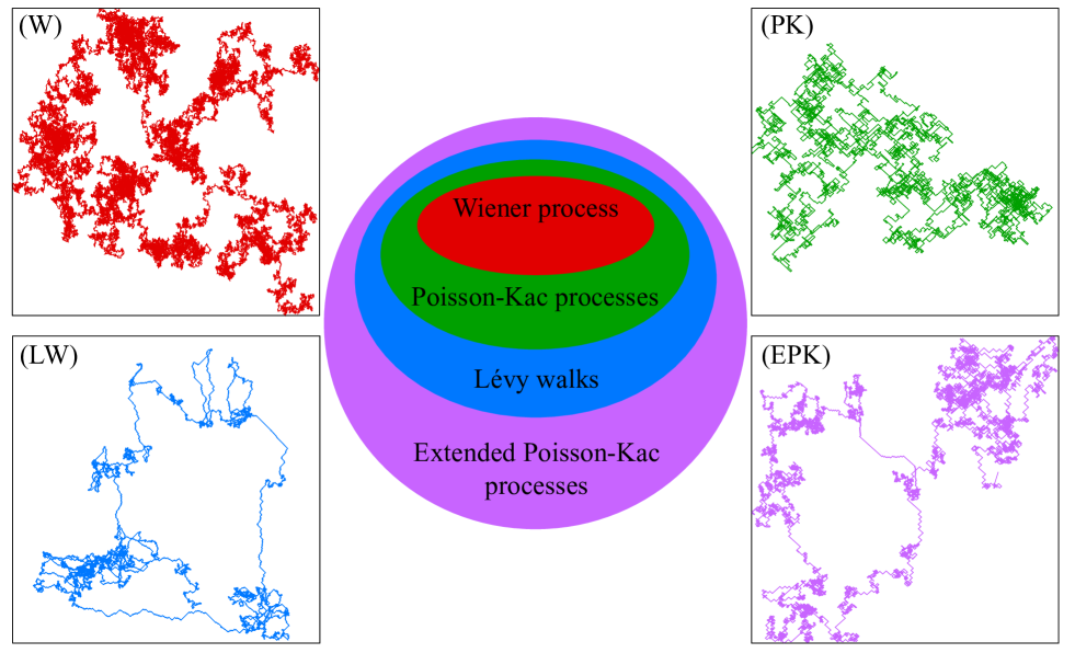
Figure 1: Schematic representation of the increasing level of generalisation in stochastic kinematics with finite propagation speed, from Wiener processes (W), to Poisson-Kac processes (PK), to Lévy walks (LW), and finally to extended Poisson-Kac processes (EPK). The latter define the new class of stochastic models introduced in Section III. Overlapping Poisson-Kac processes, which are discussed specifically in Subsec. III.2, are one particular instance of these processes. Example orbits of realisations of these processes in two spatial dimensions are shown correspondingly. For two-dimensional LWs, we simulate the two-state model (see Subsec. II.3) with the transition rate Eq. (7) where $\xi=1.5$. For the class of EPK processes we choose a senescent LW (see Subsec. IV.1) with $\xi=1$ and $\tau^{0}=1$.

II.4 Dissecting the structure of Poisson-Kac processes

Let us reconsider the process defined by Eq. (1). In fully general terms, this involves a set of state variables $\Sigma_{X}$, which in our specific case only contains the process $X(t)$ itself (note that upper case letters refer to the stochastic processes, while lower case to their realisation). These state variables are defined in some prescribed domain ${\mathcal{D}}_{X}\subseteq{\mathbb{R}}^{n}$, with $n$ being the total number of such variables. In the case considered here, ${\mathcal{D}}_{X}={\mathbb{R}}$. The dynamics of these state variables is controlled by a set of driving stochastic processes, also called transitional parameters, $\Sigma_{T}$, which can assume values in the set $D_{T}\subseteq{\mathbb{R}}^{m}$, with $m$ being the total number of such values. The transitional parameters are chosen such that their joint process with the state variables is Markovian, while instead the state variables alone are non-Markovian. For Eq. (1), in particular, the only transitional parameter is the process $S(t)=(-1)^{\chi(t,\lambda)}$, which attains values in $D_{T}=\{-1,1\}$. In agreement with the condition above, we have shown previously that, while $X(t)$ alone is non-Markovian, the couple $(X(t),S(t))$ is Markovian instead. The dynamics of the state variables may also depend on a set of physical parameters $\Sigma_{P}$, such as $b$ and $\lambda$ for the PK process Eq. (1), generically defined in the domain ${\mathcal{D}}_{P}\in{\mathbb{R}}^{p}$, with $p$ being the dimensionality of these parameters. Finally, the stochastic dynamic is given as a vector field $f:{\mathcal{D}}_{X}\times{\mathcal{D}}_{T}\times{\mathcal{D}}_{P}\rightarrow{\mathcal{D}}_{X}$, expressing the temporal evolution of the state variables and depending on the elements of the set $\Sigma_{X}\cup\Sigma_{T}\cup\Sigma_{P}$. Within this framework, it becomes clear how we can formulate correctly the primitive statistical description of this dynamic. This is achieved in terms of the PPDW functions of the state variables, which are additionally parametrised by the attainable values of the transitional parameters, owing to the Markovian recombination mechanism that they provide.

According to this framework, in its essence the structure of a PK process is constituted by the system $(\Sigma_{X},\Sigma_{T},\Sigma_{P},f)$, where $\Sigma_{X}=\{X\}$, $\Sigma_{T}=\{S\}$, $\Sigma_{P}=\{b,\lambda\}$ and $f$ is specified by Eq. (1). The transitional parameter $S$ parametrises the statistical description of the process, thus determining the system of PPDW functions $p(x,t;s)$, $s\in D_{T}=\{-1,1\}$. In our previous discussion, to simplify the notation, we have identified $p(x,t;1)=P_{+}(x,t)$ and $p(x,t,-1)=P_{-}(x,t)$. The statistics of the process is then fully determined by the Markovian evolution equations (15) for the PPDW functions.

III From Lévy walks to extended Poisson-Kac processes

Motivated by the connection between LWs and PK processes just established through the PPDW approach, in this section we formalise the family of EPK processes, the new class of stochastic processes with finite propagation speed that constitute the fourth layer of generalisation in Fig. 1. All the other processes discussed so far can thus be recovered from them as special cases. We choose this terminology to distinguish them from the generalised PK processes previously discussed in the literature Giona et al. (2017a); Giona (2017); Giona et al. (2017b). In fact, these processes can be obtained within our formalism.

First, we define the concept of overlap. This consists in introducing an additional coordinate to the classical description of PK processes. This coordinate is a state variable that can be interpreted as an internal time representing the transitional age of the process, i.e., the time elapsed from the last velocity transition. Simultaneously, this coordinate also plays the role of a transitional parameter, as it directly controls the stochastic machinery of the random velocity switches. We call this coordinate overlapping, as it belongs to both sets $\Sigma_{X}$ and $\Sigma_{T}$. The overlapping variable undergoes deterministic dynamics between different transitions and discontinuous Markovian jumps at each transition instants. Remarkably, we demonstrate that this formalism can capture a generic functional form for the transition time PDF, such as the power law tailed Eq. (5) characteristic of LW processes. This coupling between the state variables and the driving stochastic processes is therefore the key ingredient in order to embed LWs within a generalised theory of PK processes. We then derive the statistical description of general overlapping PK processes in terms of partial differential equations for their PPDW functions. These processes are however not the most general form of stochastic processes with finite propagation velocities and transition rates. For overlapping PK processes, in fact, the Markovian jump dynamics of the overlapping and state variables is assumed to be fully synchronised by definition. Clearly, different processes can be obtained if we relax this condition, e.g., by fully desynchronising the transitional dynamics of overlapping and state variables. In fact, we provide a recipe for how the transitional synchronisation between these processes can be modelled explicitly. We denote as EPK processes the stochastic models generated within this framework.

III.1 Formulating a stochastic equation for generalised Poisson-Kac processes

With the knowledge of the PPDW approach (see Sec. II.3) it is worthwhile to return to the basic stochastic equation of motion (1) defining the classical one-dimensional PK process. This equation yields PK dynamics by using a constant transition rate $\lambda$ for the corresponding Poisson counting process $\chi(t,\lambda)$. In contrast to this, Eq. (6), which was used to define the transition time PDF $T(\tau)$ more generally, involves a generalised transition rate $\lambda(\tau)$ that depends on the transition time $\tau$. This simple observation of having intrinsically different transition rates for PK processes and LWs suggests that LWs can be expressed in the form of the suitably amended PK process

$$\mathop{}\!\mathrm{d}x(t) = b\,(-1)^{\chi(t,\lambda(\tau(t)))}\,\mathop{}\!\mathrm{d}t\>,$$ (16)

$$\mathop{}\!\mathrm{d}\tau(t) = \mathop{}\!\mathrm{d}t\>.$$ (17)

Here $\chi(t,\lambda(\tau))$ represents a generalised Poisson process whose transition rate $\lambda$ depends generically on the value attained by the additional coordinate $\tau$, the transitional age, which stands for the time elapsed after the last velocity transition. In turn, $\tau$ is coupled to the physical time $t$ by Eq. (17). For example, using the time-dependent transition rate Eq. (7) yields a generalised Poisson process characterised by the power law transition time PDF Eq. (5) .

Equations (16) and (17) are only valid in the time interval between two velocity transitions. In order to extend them over the entire history of the process, we need to supplement them with boundary conditions at the transition times. Intuitively, these boundary conditions must involve the auxiliary variable $\tau$ and be discontinuous. In fact, whenever a transition in $\chi(t,\lambda(\tau(t)))$ occurs, the transitional age $\tau$ is reset to zero. In contrast, because the transition only changes the velocity direction, the stochastic process $x(t)$ is continuous at the transition time. In mathematical terms, assuming that a transition occurs at the time instant $t^{*}$, we then set

$$x(t^{*}_{+})=x(t_{-}^{*})\>\quad\mbox{and}\quad\>\tau(t^{*}_{+})=0\>,$$ (18)

with the shorthand notation $f(t^{*}_{\pm})=\lim_{\epsilon\to 0}f(t^{*}\pm\epsilon)$ and $f$ any smooth or continuous function. For the transition rate Eq. (7) the PK process defined by Eqs. (16) and (17) equipped with the boundary conditions Eq. (18) generates a LW dynamics. This is demonstrated formally by calculating the evolution equations for the PPDW functions of the process $x$, which can be shown to be equal to Eqs. (8) (see Subsec. C). Within this setting, a LW can therefore be interpreted as a form of non-autonomous PK process depending explicitly on the internal time coordinate $\tau$.

The observations above further suggest that LWs can be reformulated within the theory of PK processes by defining the new state variable

$${\bf y}=\left(\begin{array}[]{c}x\\ \tau\end{array}\right)\>.$$ (19)

This formulation is analogous to the lift of the time coordinate that is employed to transform a non-autonomous one-dimensional dynamical system into an autonomous one in two dimensions Strogatz (2018). It thus trivially leads to studying these processes in a space of dimension higher than one, for which we will adapt the generalisation of the theory of PK processes to higher dimensional state spaces described in Refs. Giona et al. (2017a, c, d). We note that this reformulated process belongs to the well-known class of renewal processes Cox (1962), which presents a big advantage. Since our process $x$ only admits two states with velocities $\pm b$, for the lifted state variable ${\bf y}$ we define the two generalised velocity vectors

$${\bf b}(1)=\left(\begin{array}[]{c}b\\ 1\end{array}\right)\;,\qquad{\bf b}(-1)=\left(\begin{array}[]{c}-b\\ 1\end{array}\right)\>.$$ (20)

Using the setting Eqs. (19) and (20), and assuming $\lambda$ to only depend on the transitional age variable $\tau$, the equations of motion (16) and (17) can be compactly expressed as

$$\mathop{}\!\mathrm{d}{\bf y}(t)={\bf b}\left((-1)^{\chi(t,\lambda(\tau(t)))}\right)\,\mathop{}\!\mathrm{d}t\>,$$ (21)

equipped with the boundary conditions Eqs. (18) at each time instant when a state transition occurs. More general choices are also possible. For example, if we assume the dynamics of the transitional age ${\mathcal{T}}(t)$ to be a stochastic process possessing a Markovian transitional structure, the boundary condition for $\tau(t^{*}_{+})$ becomes

$$\tau(t^{*}_{+}) = \tau^{\prime}\qquad\mbox{with probability }\;k(\tau^{\prime},\tau(t^{*}_{-}))\;\>.$$ (22)

Evidently, we need to assume the following conditions on the transition probability $k(\tau^{\prime},\tau)$, i.e,

$$k(\tau^{\prime},\tau)\geq 0\qquad\mbox{and}\qquad\int_{-\infty}^{\infty}k(\tau^{\prime},\tau)\,d\tau^{\prime}=1\>.$$ (23)

The particular case of Eq. (18) corresponds to setting $k(\tau^{\prime},\tau)=\delta(\tau^{\prime})$.

The formulation provided by Eqs. (19), (20) and (21) elucidates the following characteristic features of the multivariate process ${\bf Y}(t)$: On the one hand, it possesses an evident skew product structure, because we can formally write ${\bf Y}(t)=(X(t;{\mathcal{T}}(t)),{\mathcal{T}}(t))$. In fact, while the transitional age process ${\mathcal{T}}(t)$ does not incorporate the position process $X(t)$, the latter, in contrast, depends explicitly on time $t$ and is simultaneously a nonlinear functional of ${\mathcal{T}}(t)$ through the Poissonian transition rate $\lambda$. On the other hand, in Eq. (21) the noise is manifestly governed by the state variable $\tau$. This coupling thus modulates the very fundamental stochastic structure of the fluctuations, as is made evident by the fact that the transition rate $\lambda(\tau)$ controls the correlation properties of the resulting dynamics . These properties reveal a striking change of paradigm with respect to conventional PK processes, which is determined by the overlap between the state variable ${\bf y}$ and the transitional parameters controlling the randomisation dynamics as just described. This peculiar feature defines a new class of stochastic processes with finite propagation velocity, called overlapping PK processes (OPK), that includes LWs as a special case.

III.2 Overlapping Poisson-Kac processes

We now formalise the concept of overlap introduced previously by specifying the formal structure of the multivariate stochastic process Y(t) (see Subsec. II.4). In fully general terms, we define a PK process to be overlapping if the following conditions hold true: (i) The sets of state variables, $\Sigma_{X}$, and of transitional parameters, $\Sigma_{T}$, possess a non-empty intersection,

$$\Sigma_{O}=\Sigma_{X}\cap\Sigma_{T}\neq\emptyset\>.$$ (24)

(ii) The transition dynamics of the variables in $\Sigma_{T}$ depend exclusively on the dynamics of those in its set complementary to $\Sigma_{O}$, i.e., the set $\Sigma_{T}/\Sigma_{O}$, which contains all variables belonging to $\Sigma_{T}$ but not to $\Sigma_{O}$. Furthermore, we assume the dynamics of these variables to be Markovian. We acknowledge that non-Markovian dynamics for these variables can also be considered but will not be discussed in this context. These two properties imply that the transitional mechanism of an OPK process is essentially controlled by the Markovian transition dynamics of the variables in $\Sigma_{T}/\Sigma_{O}$, while those in $\Sigma_{O}$ are characterised by a smooth evolution equation unless when a transition occurs, at which time instant they perform discontinuous jumps. In this overlapped transition process, all the physical parameters characterising the Markovian dynamics of the variables in $\Sigma_{T}/\Sigma_{O}$ can be potentially modulated not only by the local state of the variables in $\Sigma_{O}$, but also by that of the state variables belonging to $\Sigma_{X}$.

This is the basic mechanism characterising the evolution of a LW process, as defined by Eqs. (16) and (17) with the boundary conditions Eq. (18). For this stochastic model we have $\Sigma_{X}=\{{\bf Y}\}=\{X,\mathcal{T}\}$ and $\Sigma_{T}=\{S,\mathcal{T}\}$, with the generalised Poisson process $S(t)=(-1)^{\chi(t,\lambda(\tau(t)))}$. Consequently, we identify $\Sigma_{O}=\{\mathcal{T}\}$ and $\Sigma_{T}/\Sigma_{O}=\{S\}$. In agreement with our previous argument, in a LW therefore the transitional age process $\mathcal{T}$ exhibits a smooth temporal dynamic (a linear growth in this specific case) except for randomly distanced discontinuities occurring at all times when the transitional parameter $S$ performs a transition (here specifically a sign flip).

With these definitions at our disposal, we can now derive the statistical characterisation of a general OPK process. To keep our formalism general, we assume $n$ spatial dimensions for the position process, ${\bf X}(t)$, with domain ${\mathcal{D}}_{X}\subseteq{\mathbb{R}}^{n}$, and $m\leq n$ dimensions for the overlapped variables, $\boldsymbol{\mathcal{T}}(t)$, with domain ${\mathcal{D}}_{\tau}\subseteq{\mathbb{R}}^{m}$. Correspondingly, we set $\Sigma_{X}=\{{\bf Y}\}=\{{\bf X},\boldsymbol{\mathcal{T}}\}$. Stochasticity is generated in the model by defining a set of $n$-dimensional velocity vectors ${\bf b}(\boldsymbol{\alpha})$, which depend on a stochastic parameter $\boldsymbol{\alpha}\in{\mathcal{D}}_{\alpha}\subseteq{\mathbb{R}}^{d}$ ($d=1,2,\dots,n$). The set ${\mathcal{D}}_{\alpha}$ can be either discrete or continuous, thus providing us with several modelling opportunities for the underlying stochastic dynamics of the overlapping PK process. The stochastic temporal evolution of these variables is specified by introducing a Poisson field $\boldsymbol{\Xi}(t;\lambda,A)$ in ${\mathbb{R}}^{d}$, such that

$$\boldsymbol{\alpha}(t)=\boldsymbol{\Xi}(t;\lambda,A)\>,$$ (25)

where $\boldsymbol{\Xi}(0;\lambda,A)=\boldsymbol{\alpha}_{0}\in{\mathcal{D}}_{\alpha}$. The Poisson field is a continuous stochastic process attaining values in ${\mathcal{D}}_{\alpha}$ whose statistical description satisfies a continuous Markov chain dynamics defined by the transition rate function $\lambda\geq 0$ and by the transition probability kernel $A$. We specify the functional dependence of these parameters below; further details on Poisson fields are given in Appendix B. In this setting, we therefore define $\Sigma_{T}=\{\boldsymbol{\Xi},\boldsymbol{\mathcal{T}}\}$, $\Sigma_{O}=\{\boldsymbol{\mathcal{T}}\}$ and $\Sigma_{T}/\Sigma_{O}=\{\boldsymbol{\Xi}\}$.

Finally, we assume for the lifted process ${\bf Y}(t)$ the following stochastic differential equation,

$$\mathop{}\!\mathrm{d}{\bf y}(t)=\widetilde{\bf v}({\bf y}(t))\,\mathop{}\!\mathrm{d}t+\widetilde{\bf b}(\boldsymbol{\Xi}(t),{\bf y}(t))\,\mathop{}\!\mathrm{d}t\>,$$ (26)

where we introduced a deterministic biasing velocity field and a stochastic perturbation defined as, respectively,

$$\widetilde{\bf v}({\bf y})=\left(\begin{array}[]{c}{\bf v}({\bf x},\boldsymbol{\tau})\\ {\bf w}({\bf x},\boldsymbol{\tau})\end{array}\right)\,,\qquad\widetilde{\bf b}(\boldsymbol{\alpha},{\bf y})=\left(\begin{array}[]{c}{\bf b}(\boldsymbol{\alpha},{\bf x},\boldsymbol{\tau})\\ 0\end{array}\right)\>.$$ (27)

The stochastic velocity vectors ${\bf b}:{\mathcal{D}}_{\alpha}\times{\mathcal{D}}_{X}\times{\mathcal{D}}_{\tau}\mapsto{\mathbb{R}}^{n}$, parametrised with respect to the states $\boldsymbol{\alpha}$ of the Poisson field $\boldsymbol{\Xi}(t)$, are also further modulated by an explicit dependence on the model state variables. If we neglect this dependence of the stochastic perturbation on the state variables and the deterministic field $\widetilde{\bf v}$, and we identify the Poisson field $\boldsymbol{\Xi}(t)$ with $S(t)$, Eq. (27) is fully analogous to Eq. (21). In addition, even the constitutive properties of the Poisson field $\boldsymbol{\Xi}(t)$, i.e., the transition rate $\lambda$ and the probability kernel $A$, can be specified more generally as depending on the variables belonging to the set $\Sigma_{X}\cup\Sigma_{T}$, i.e.,

$$\lambda = \lambda({\bf x},\boldsymbol{\tau},\boldsymbol{\alpha})\>,$$ (28)

$$A = A({\bf x},\boldsymbol{\alpha},\boldsymbol{\tau},\boldsymbol{\alpha}^{\prime},\boldsymbol{\tau}^{\prime})\>.$$ (29)

The local functional dependence of the kernel $A$ on the state variables ${\bf x}$ preserves the validity of a locality principle for the stochastic process ${\bf X}(t)$, i.e., non-local action at distance is not allowed in our model. This would not be preserved if $A$ also depended on ${\bf x}^{\prime}$; if such a dependence existed, it would in fact imply the possible occurrence of discontinuous spatial jumps ${\bf x}^{\prime}\mapsto{\bf x}$. At each transition time $t^{*}$ of the Poisson field $\boldsymbol{\Xi}$, we equip Eq. (26) with the boundary condition

$$\boldsymbol{\tau}(t^{*}_{+}) = \boldsymbol{\tau}^{\prime}\qquad\mbox{with probability }\;A({\bf x}(t^{*}_{-}),\boldsymbol{\alpha},\boldsymbol{\tau}(t^{*}_{-}),\boldsymbol{\alpha}^{\prime},\boldsymbol{\tau}^{\prime})\;\>.$$ (30)

Eqs. (26) and (27) explictly state that in any time interval in which no transitions in the Poisson field $\boldsymbol{\Xi}(t)$ occur, the dynamics of the overlapped variable $\boldsymbol{\mathcal{T}}(t)$ follows a strictly deterministic kinematics. In agreement with our previous arguments, the overlapped variables thus do not depend explicitly on the main transitional parameter, here $\boldsymbol{\Xi}(t)$, but only implicitly through its transition dynamics. Moreover, we remark that if $A({\bf x},\boldsymbol{\alpha},\boldsymbol{\tau},\boldsymbol{\alpha}^{\prime},\boldsymbol{\tau}^{\prime})$ is different from zero for $\boldsymbol{\tau}\neq\boldsymbol{\tau}^{\prime}$, at any transition instant of the stochastic process $\boldsymbol{\Xi}(t)$ the overlapped variables $\boldsymbol{\mathcal{T}}(t)$ may perform a discontinuous jump $\boldsymbol{\tau}^{\prime}\mapsto\boldsymbol{\tau}$. Consequently, $\boldsymbol{\mathcal{T}}(t)$ can display nonlocal dynamics, which is fully consistent with the locality principle of space-time interactions, provided that the ${\boldsymbol{\tau}}$ variables do not correspond to any space-time coordinate or physical field (otherwise the principle of bounded propagation velocity would be violated) but solely internal non-geometrical variables of the system (such as the transitional age).

The statistical characterisation of Eq. (26) is formally identical to that of conventional generalised PK processes that has been derived in Refs. Giona et al. (2017a, c, d). In our case this is obtained in terms of the PPDW functions $p({\bf y},t,\boldsymbol{\alpha})=p({\bf x},\boldsymbol{\tau},t,\boldsymbol{\alpha})$. Introducing the notation ${\bf x}=(x_{1},\dots,x_{n})$, $\boldsymbol{\tau}=(\tau_{1},\dots,\tau_{m})$, $\nabla_{\bf x}=(\partial_{x_{1}},\dots,\partial_{x_{n}})$ and $\nabla_{\boldsymbol{\tau}}=(\partial_{\tau_{1}},\dots,\partial_{\tau_{m}})$, and assuming the domains $\mathcal{D}_{\tau}$ and $\mathcal{D}_{\alpha}$ to be continuous, we obtain the evolution equation

$$\frac{\partial p({\bf x},\boldsymbol{\tau},t,\boldsymbol{\alpha})}{\partial t} =-\nabla_{\bf x}\cdot\left[{\bf v}({\bf x},\boldsymbol{\tau})\,p({\bf x},\boldsymbol{\tau},t,\boldsymbol{\alpha})\right]-\nabla_{\bf x}\cdot\left[{\bf b}({\bf x},\boldsymbol{\tau},\boldsymbol{\alpha})\,p({\bf x},\boldsymbol{\tau},t,\boldsymbol{\alpha})\right]-\nabla_{\boldsymbol{\tau}}\cdot\left[{\bf w}({\bf x},\boldsymbol{\tau})\,p({\bf x},\boldsymbol{\tau},t,\boldsymbol{\alpha})\right]$$

$$\quad-\lambda({\bf x},\boldsymbol{\tau},\boldsymbol{\alpha})\,p({\bf x},\boldsymbol{\tau},t,\boldsymbol{\alpha})+\int_{{\mathcal{D}}_{\tau}}\left[\int_{{\mathcal{D}}_{\alpha}}\lambda({\bf x},\boldsymbol{\tau}^{\prime},\boldsymbol{\alpha}^{\prime})A({\bf x},\boldsymbol{\alpha},\boldsymbol{\tau},\boldsymbol{\alpha}^{\prime},\boldsymbol{\tau}^{\prime})\,p({\bf x},\boldsymbol{\tau}^{\prime},t,\boldsymbol{\alpha}^{\prime})\,\mathop{}\!\mathrm{d}\boldsymbol{\alpha}^{\prime}\right]\mathop{}\!\mathrm{d}\boldsymbol{\tau}^{\prime}\>,$$ (31)

where

$$\int_{{\mathcal{D}}_{\tau}}\left[\int_{{\mathcal{D}}_{\alpha}}A({\bf x},\boldsymbol{\alpha},\boldsymbol{\tau},\boldsymbol{\alpha}^{\prime},\boldsymbol{\tau}^{\prime})\,\mathop{}\!\mathrm{d}\boldsymbol{\alpha}\right]\mathop{}\!\mathrm{d}\boldsymbol{\tau}=1$$ (32)

for any $\boldsymbol{\tau}^{\prime}\in{\mathcal{D}}_{\tau}$ and $\boldsymbol{\alpha}^{\prime}\in{\mathcal{D}}_{\alpha}$. Likewise, if the set $\mathcal{D}_{\alpha}$ is discrete, Eqs. (31) and (32) still hold with the corresponding integral terms suitably substituted by summations. We note that, in this case, the function $p({\bf x},\boldsymbol{\tau},t,\boldsymbol{\alpha})$ is to be interpreted as a probability (not a density) with respect to the stochastic variables $\boldsymbol{\alpha}$. It is straightforward to show that this general framework can generate LW dynamic as a special case, see Appendix C for the derivation.

III.3 Transitional asynchrony lines the route to extended Poisson-Kac processes

We now develop our EPK theory in its most general form by introducing the concept of transitional asynchrony. Let us illustrate this concept by reconsidering the dynamics of the variable $\boldsymbol{\tau}$, which we have introduced for LWs to denote the transitional age. We now assume that $\boldsymbol{\tau}$ follows a Markovian transition dynamics with rate $\mu({\bf x},\boldsymbol{\tau})$ and transition probability kernel $M({\bf x},\boldsymbol{\tau},\boldsymbol{\tau}^{\prime})$ (see Appendix B). By construction, this is a left stochastic kernel, i.e., $M({\bf x},\boldsymbol{\tau},\boldsymbol{\tau}^{\prime})\geq 0$, $\int_{{\mathcal{D}}_{\tau}}M({\bf x},\boldsymbol{\tau},\boldsymbol{\tau}^{\prime})\,\mathop{}\!\mathrm{d}\boldsymbol{\tau}=1$ for all $\boldsymbol{\tau}^{\prime}\in{\mathcal{D}}_{\tau}$. Potentially, a further deterministic evolution can be superimposed to this Markovian transitional dynamics. Here for simplicity we keep the same one as in Eqs. (26) and (27). The stochastic equation of motion for the state variable ${\bf x}(t)$ is equal to that encapsulated in Eq. (26). Its statistical description involves the PPDW functions $p({\bf x},t,\boldsymbol{\alpha},\boldsymbol{\tau})$, where now both $\boldsymbol{\alpha}$ and $\boldsymbol{\tau}$ are to be interpreted as stochastic parameters, which are solutions of the hyperbolic equations (as expressed in the form of first order equations with respect to time $t$, position ${\bf x}$ and $\boldsymbol{\tau})$

$$\frac{\partial p({\bf x},\boldsymbol{\tau},t,\boldsymbol{\alpha})}{\partial t} =-\nabla_{\bf x}\cdot\left[{\bf v}({\bf x},\boldsymbol{\tau})\,p({\bf x},\boldsymbol{\tau},t,\boldsymbol{\alpha})\right]-\nabla_{\bf x}\cdot\left[{\bf b}({\bf x},\boldsymbol{\tau},\boldsymbol{\alpha})\,p({\bf x},\boldsymbol{\tau},t,\boldsymbol{\alpha})\right]-\nabla_{\boldsymbol{\tau}}\cdot\left[{\bf w}({\bf x},\boldsymbol{\tau})\,p({\bf x},\boldsymbol{\tau},t,\boldsymbol{\alpha})\right]$$

$$\quad-\lambda({\bf x},\boldsymbol{\tau},\boldsymbol{\alpha})\,p({\bf x},\boldsymbol{\tau},t,\boldsymbol{\alpha})+\int_{{\mathcal{D}}_{\alpha}}\lambda({\bf x},\boldsymbol{\tau},\boldsymbol{\alpha}^{\prime})A({\bf x},\boldsymbol{\alpha},\boldsymbol{\tau},\boldsymbol{\alpha}^{\prime},\boldsymbol{\tau})\,p({\bf x},\boldsymbol{\tau},t,\boldsymbol{\alpha}^{\prime})\,\mathop{}\!\mathrm{d}\boldsymbol{\alpha}^{\prime}$$

$$\quad-\mu({\bf x},\boldsymbol{\tau})\,p({\bf x},\boldsymbol{\tau},t,\boldsymbol{\alpha})+\int_{{\mathcal{D}}_{\tau}}\mu({\bf x},\boldsymbol{\tau}^{\prime})M({\bf x},\boldsymbol{\tau},\boldsymbol{\tau}^{\prime})\,p({\bf x},\boldsymbol{\tau}^{\prime},t,\boldsymbol{\alpha})\,\mathop{}\!\mathrm{d}\boldsymbol{\tau}^{\prime}\>,$$ (33)

In formal terms, this generalised PK process is specified by the sets of state and transitional variables $\Sigma_{X}=\{{\bf X}\}$ and $\Sigma_{T}=\{\boldsymbol{\Xi},\boldsymbol{\mathcal{T}}\}$, respectively. In contrast, the overlapping PK process Eq. (26) is defined by the sets $\Sigma_{X}=\{{\bf X},\boldsymbol{\mathcal{T}}\}$ and $\Sigma_{T}=\{\boldsymbol{\Xi},\boldsymbol{\mathcal{T}}\}$. Interestingly, these two different formal structures (in particular, characterised by different transitional mechanisms) lead to different statistical properties (compare Eqs. (31) and (33)). Both are characterised by the interplay of the main transitional parameters $\boldsymbol{\Xi}(t)$ and $\boldsymbol{\mathcal{T}}(t)$ to determine the stochastic dynamic of the position process ${\bf X}(t)$. The difference between the two formulations is a consequence of the different synchronisation between the processes $\boldsymbol{\Xi}$ and $\boldsymbol{\mathcal{T}}$. This concept is made evident by defining for each of the two transitional parameters the marginal transition time density, $T_{\boldsymbol{\Xi}}(t_{1})$ and $T_{\boldsymbol{\mathcal{T}}}(t_{2})$, respectively. Likewise, for the joint process $(\boldsymbol{\Xi}(t),\boldsymbol{\mathcal{T}}(t))$ we can specify the corresponding bivariate transition time density function $T_{\boldsymbol{\Xi},\boldsymbol{\mathcal{T}}}(t_{1},t_{2})$. Correspondingly, we can define the conditional transitional time density, $T_{\boldsymbol{\mathcal{T}}|\boldsymbol{\Xi}}(t_{2}\,|\,t_{1})$, by the relation

$$T_{\boldsymbol{\Xi},\boldsymbol{\mathcal{T}}}(t_{1},t_{2})=T_{\boldsymbol{\mathcal{T}}|\boldsymbol{\Xi}}(t_{2}\,|\,t_{1})\,T_{\boldsymbol{\Xi}}(t_{1})\>.$$ (34)

This quantity elucidates the different physics underlying the generalised PK process defined by Eqs. (33) and the OPK process Eq. (31). For the former

$$T_{\boldsymbol{\mathcal{T}}|\boldsymbol{\Xi}}(t_{2}\,|\,t_{1})=T_{\boldsymbol{\mathcal{T}}}(t_{2})\>,$$ (35)

meaning that the processes $\boldsymbol{\Xi}(t)$ and $\boldsymbol{\mathcal{T}}(t)$ are transitionally independent. Clearly, in this case the variable $\boldsymbol{\tau}$ loses its physical meaning of an elapsed time from the previous transition. For the latter

$$T_{\boldsymbol{\mathcal{T}}|\boldsymbol{\Xi}}(t_{2}\,|\,t_{1})=\delta(t_{2}-t_{1})\>,$$ (36)

i.e., the two processes are transitionally synchronised. In this case, $\boldsymbol{\tau}$ is indeed an elapsed time, or transitional age.

Remarkably, all the previous considerations can be applied as well to any model parameters. For simplicity, let us consider a one-dimensional PK process (extending these arguments to the three-dimensional setting is straightforward), which is specified formally by the sets of state variables, transitional parameters and model parameters $\Sigma_{X}=\{X\}$, $\Sigma_{T}=\{S\}$ and $\Sigma_{P}=\{b,\lambda\}$, respectively. We then assume $b=b_{0}\beta(t)$ and $\lambda=\lambda_{0}\lambda(t)$. A new family of EPK processes can then be obtained by considering a subset of the model parameters as transitional variables, i.e., $\Sigma_{X}=\{X\}$, $\Sigma_{T}=\{S,\Lambda,B\}$, $\Sigma_{P}=\{b_{0},\lambda_{0}\}$. Similarly, a new family of OPK processes can be obtained by considering them as both state and transitional variables, i.e., $\Sigma_{X}=\{X,B,\Lambda\}$, $\Sigma_{T}=\{S,B,\Lambda\}$, $\Sigma_{P}=\{b_{0},\lambda_{0}\}$. Each of these classes of finite propagation velocity processes are characterised by different transitional structures, thus leading to different statistical properties. However, the argument above highlights that these two processes are particular cases of a wider class of models, where transitional asynchronies between the state variables and the main generator of microscopic stochasticity are encapsulated in the transitional time conditional density, for the example considered $T_{\{\beta,\Lambda\}|S}$.

We denote these general models of stochastic dynamics with finite propagation velocity as EPK processes. The formulation of EPK theory that includes OPK processes (and LWs among them) as special cases is our second main result. Figure 1 pictorially describes the inclusive relationship between the main classes of stochastic kinematics formulated so far. The common denominator between all these stochastic models, except for Wiener processes (which are in this sense a singular limit), is the assumption of a finite propagation speed and finite transition rates. The main difference resides in the statistics of the transition times, which is exponential for PK processes, power law tailed for LWs and fully generic for EPK processes; and in the existence (or absence) of transitional asynchronies among the state variables and the microscopic stochastic generator.

This analysis elucidates the physical meaning and the broad range of applications of our extension of conventional PK theory. Transitionally independent PK models generically yield microscopic processes subjected to external (environmental) fluctuations that influence their local dynamics, but they can be considered independent of the fluctuations in the local microscopic motion. Conversely, OPK models capture complex microscopic fluctuations, the statistical description of which requires the introduction of inner transitionally synchronised degrees of freedom. This is for example the case of the transitional age $\tau$ for LW processes. In between these two limiting cases, a spectrum of intermediate situations can be defined ad hoc, by specifying the transitional time conditional density between the state variables and the main transitional process.

IV Extended Poisson-Kac processes: case studies

We now discuss three specific examples of one-dimensional EPK processes. First, we introduce a transitional senescent random walk, where the transitional dynamic depends explicitly on the number of total transitions already occurred. We specifically study an EPK model where the age to which the walker is reset following a velocity transition is parametrised as an increasing function of the total number of transitions. Second, we discuss an EPK model that can reproduce “Brownian yet non Gaussian” diffusion Wang et al. (2012a). This behaviour can be obtained by considering an EPK process where the walker velocity follows a Markovian jump dynamic transitionally independent from the corresponding dynamic of the Poisson field. Differently from other phenomenological approaches Chechkin et al. (2017), our model provides a clear microscopic interpretation of this dynamics. Finally, we formulate an EPK process with correlated transitional dynamic. If these correlations are neglected, the model generates LW dynamic. If the correlations lead to increasing transition rates over time, the model yields a dynamic characterised by a sub- to superdiffusive crossover in the mean square displacement. The variety of diffusive dynamics that can be captured by EPK processes highlights the modelling power of our theory. We remark that in this work we only discuss examples of OPK and transitionally independent EPK processes. The analysis of further EPK processes, requiring the occurrence of more non-trivial multivariate distributions of joint transition times (which is an intricate problem even for finite Markov chains Bielecki et al. (2012, 2017) and associated counting processes Karlis and Xekalaki (2005)) will be developed in future communications.

IV.1 Transitional Senescent Random Walks

In 1961 Hayflick and Moorhead reported that cultured proliferating human diploid cells stop cellular division after a limited number of mytotic events Hayflick and Moorhead (1961); Hayflick (1965) showing that this phenomenon is related to senescence, i.e. to aging process occurring at a cellular level Harley et al. (1990); Krtolica et al. (2001). Apart from its biological and biochemical relevance, senescence is remarkable from a statistical mechanical perspective, where it translates to the formulation of random walk processes whose dynamic and transitional properties can decay as the number of transitions increases. In analogy with the terminology established in the biological context, we call this feature transitional senescence. Correspondingly, we refer to transitionally senescent random walk processes implementing this feature. A particular example has been discussed in the context of LWs in Ref. Giona et al. (2019a), where a progressive decrease of the walker velocity $b$ with the number of transitions has been shown to yield qualitative effects for the statistics of motion. Here we show how this feature can be easily accommodated within our general theory of EPK processes.

Transitional senescence can be represented by the fact that either the transition rate $\lambda$ and/or the walker velocity $b$ can become functions of the underlying stochastic counting process $N(t)$, associated with the Markovian transitional structure of the process. The process $N(t)$ enumerates the transitions occurred up to the time interval $[0,t)$. As a pedagogical example, we consider first the case of a general transitionally senescent PK process. The system of transitional parameters for this process is $\Sigma_{T}=\{S,N\}$. Moreover, the system of state variables is $\Sigma_{X}=\{X,N\}$, albeit the dynamics of $N(t)$ is elementary. In fact, $\mathop{}\!\mathrm{d}N(t)/\mathop{}\!\mathrm{d}t=0$ in any time interval between two transitions, and $N(t)\mapsto N(t)+1$ at any transition instant. Because counting process $N(t)$ is transitionally synchronised with $S(t)$, this is for all intents and purposes an OPK process. Its statistical description involves the family of PPDW functions $p_{s}^{(n)}(x,t)\equiv p(x,n,t,s)$ with $s=\pm$ and $n\in{\mathbb{Z}}^{\geq 0}$. To model in full generality the transitional senescence, we assume both the transition rate $\lambda_{n}$ and the velocity $b_{n}$ to be functions of the counting state $n$. The evolution equations for the associated OPK process are thus expressed by

$$\frac{\partial p_{\pm}^{(0)}(x,t)}{\partial t} = \mp b_{0}\,\frac{\partial p_{\pm}^{(0)}(x,t)}{\partial x}-\lambda_{0}\,p_{\pm}^{(0)}(x,t)\>,$$ (37)

$$\frac{\partial p_{\pm}^{(n)}(x,t)}{\partial t} = \mp b_{n}\,\frac{\partial p_{\pm}^{(n)}(x,t)}{\partial x}-\lambda_{n}\,p_{\pm}^{(n)}(x,t)+\lambda_{n-1}\,p_{\mp}^{(n-1)}(x,t)\>.$$

The generalisation to a senescent LW is now straightforward, as we just need to include the transitional age among the overlapping variables. Therefore, $\Sigma_{X}=\{X,{\mathcal{T}},N\}$, $\Sigma_{T}=\{S,{\mathcal{T}},N\}$, and thus $\Sigma_{O}=\{{\mathcal{T}},N\}$. The PPDW functions for this process are $p_{s}^{(n)}(x,\tau,t)\equiv p(x,\tau,n,t,s)$, which, similar to Eq. (37), now read

$$\frac{\partial p_{\pm}^{(0)}(x,\tau,t)}{\partial t} = \mp b_{0}\,\frac{\partial p_{\pm}^{(0)}(x,\tau,t)}{\partial x}-\frac{\partial p_{\pm}^{(0)}(x,\tau,t)}{\partial\tau}-\lambda_{0}(\tau)\,p_{\pm}^{(0)}(x,\tau,t)\>,$$ (38)

$$\frac{\partial p_{\pm}^{(n)}(x,\tau,t)}{\partial t} = \mp b_{n}\,\frac{\partial p_{\pm}^{(n)}(x,\tau,t)}{\partial x}-\frac{\partial p_{\pm}^{(n)}(x,\tau,t)}{\partial\tau}-\lambda_{n}(\tau)\,p_{\pm}^{(n)}(x,\tau,t)+\int_{0}^{\infty}k_{n}(\tau,\tau^{\prime})\,\lambda_{n-1}(\tau^{\prime})\,p_{\mp}^{(n-1)}(x,\tau^{\prime},t)\,d\tau^{\prime}\>.$$

Here the transitional senescence of the process is expressed by the Markovian transition kernels $k_{n}(\tau,\tau^{\prime})$, which are assumed to depend on the counting state $n$. The kernel $k_{n}(\tau,\tau^{\prime})$ may be an impulse Dirac delta function in $\tau$ or may admit a non-atomic support in $\tau$, consisting in an interval of values of $\tau$ for which $k_{n}(\tau,\tau^{\prime})>0$.

Equations (38) represent the statistical characterisation of a general transitionally senescent LW. To illustrate how these processes can reveal novel dynamical features, we specify the senescing process such that, after any transition, the walker transitional age is not reset to zero but to a prescribed larger value. In this respect, we introduce a diverging sequence of non-negative numbers $\{\tau_{n}^{0}\}_{n=0}^{\infty}$ with $\tau_{0}^{0}=0$ and $\tau_{n}^{0}<\tau_{n+1}^{0}$, such that

$$k_{n}(\tau,\tau^{\prime})=\delta(\tau-\tau_{n}^{0})\>,\qquad\lambda_{n}(\tau)=\lambda(\tau)\>,$$ (39)

where $\lambda(\tau)$ is specified by Eq. (7). Clearly, each $\lambda_{n}(\tau)$ is defined in the age interval $(\tau_{n}^{0},\infty)$, which implies that the corresponding transition time densities also depend on $n$. According to Eqs. (39), the age boundary conditions are

$$p_{\pm}^{(n)}(x,\tau_{n}^{0},t)=\int_{\tau_{n-1}^{0}}^{\infty}\lambda(\tau^{\prime})\,p_{\mp}^{(n-1)}(x,\tau^{\prime},t)\,\mathop{}\!\mathrm{d}\tau^{\prime}\>.$$ (40)

We simulate numerically the stochastic process associated with Eqs. (38) by further assuming constant velocities $b_{n}=b$ and $\tau_{n}^{0}=(n-1)\,\tau^{0}$ (for $n>0$), where $\tau^{0}$ is a constant positive parameter. In Fig. 2(a) we present the temporal evolution of the mean square displacement of this dynamic, $\sigma_{x}^{2}(t)=\int_{-\infty}^{\infty}x^{2}\,P(x,t)\,\mathop{}\!\mathrm{d}x$, obtained from stochastic simulations. Here we have defined the walker position distribution as $P(x,t)=\sum_{n=0}^{\infty}\sum_{s=\pm}P_{s}^{(n)}(x,t)$ with the marginal PPDW functions $P^{(n)}_{s}(x,t)=\int_{\tau_{n}^{0}}^{\infty}p_{s}^{(n)}(x,\tau^{\prime},t)\mathop{}\!\mathrm{d}\tau^{\prime}$. We simulated $10^{7}$ trajectories, all initialised at the origin, with $b=1$ and $\xi=1.5$ for different values of the parameter $\tau^{0}$. For $\tau^{0}=0$ we recover the conventional LW, in which case $\sigma_{x}^{2}(t)\sim t^{\gamma}$ with $\gamma=(3-\xi)$. In contrast, for $\tau^{0}\neq 0$ we find the different long-term scaling $\sigma_{x}^{2}(t)\sim t^{\gamma_{\rm eff}}$, characterised by the effective exponent $\gamma_{\rm eff}>\gamma$. This result is physically intuitive, because the transitional senescence induces a slowing-down in the transitional mechanism, which determines a more pronounced superdiffusive behaviour. In Fig. 2(b) we present results for $\gamma_{\rm eff}$ for different values of the parameter $\xi$ predicted by the stochastic simulations. Remarkably, we observe that $\gamma_{\rm eff}>1$ even for values $\xi>2$ for which the corresponding LW ($\tau^{0}=0$) displays an Einsteinian scaling, $\gamma=1$. For $0<\xi<1$ the senescent LW exhibits ballistic diffusion, $\gamma_{\rm eff}=2$, similar to its non-senescing counterpart. To analytically predict how $\gamma_{\text{eff}}$ depends on $\xi$ is an open problem left to further studies.

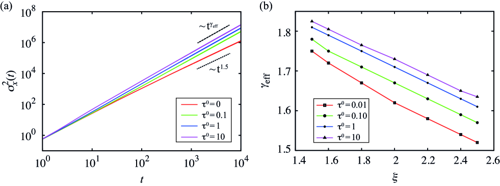
Figure 2: Superdiffusion for the model of a transitionally senescent LW, see Eq. (IV.1) and further specifications in the text. Here $\tau^{0}$ defines the senescence time. The special case $\tau^{0}=0$ corresponds to the conventional LW model without senescence. $\xi$ is the exponent of the power law distributed transition times, see Eqs. (5), respectively (7). For the speed of the walker we choose $b=1$. (a) Temporal evolution of the mean square displacement $\sigma_{x}^{2}(t)$ for $\xi=1.5$. We see that senescence enhances superdiffusion beyond the conventional LW solution. (b) The scaling exponent $\gamma_{\rm eff}$ as a function of $\xi$ increases by increasing the senescence time $\tau^{0}=0$.

IV.2 Brownian yet non-Gaussian diffusive extended Poisson-Kac processes

Brownian yet non-Gaussian diffusion is the hallmark of a specific class of transport phenomena in out-of-equilibrium systems Wang et al. (2009, 2012b). It has recently been observed, among others, for beads diffusing on lipid tubes and networks Wang et al. (2009); Toyota et al. (2011); Valentine et al. (2001); e Silva et al. (2014); Samanta and Chakrabarti (2016), for passive tracers immersed in active suspensions Leptos et al. (2009), for heterogenous populations of moving nematodes Hapca et al. (2009), and in the context of intracellular transport Witzel et al. (2009). The terminology refers generically to dynamics where the position mean square displacement scales linearly for long times, while the position statistics exhibits non-Gaussian tails. Clearly, this stochastic dynamic cannot be modelled by standard Brownian motion. Hence, the formulation of suitable stochastic processes that can capture this peculiar diffusive feature was subject to numerous theoretical investigations in recent years. According to the observation that a Laplace distribution with linearly scaling second moment can be derived from a superstatistical approach Beck and Cohen (2003), where Gaussian distributions are averaged over Laplace distributed diffusion coefficients Hapca et al. (2009), a family of “diffusing diffusivity” models has been proposed Chubynsky and Slater (2014); Chechkin et al. (2017). For these models the position process is described by standard Brownian motion with a diffusion coefficient performing a prescribed stochastic dynamic. We note that microscopic derivations of this dynamic have recently been considered in the context of active matter Kanazawa et al. (2020). Here we show that EPK processes can naturally account for the hierarchical level of fluctuations generating Brownian yet non-Gaussian diffusion by allowing the walker speed to change over time according to a given Markov chain dynamics.

For simplicity, we consider a PK process and assume $b(t)=b_{0}\,\beta(t)$, where $b_{0}>0$ is a constant parameter and $\beta(t)$ is a stochastic process attaining values in $\mathcal{D}_{\beta}=[0,b_{max}]$, which is characterised by a Markovian transition dynamics with a constant transition rate $\mu$ and the transition probability kernel $A(\beta,\beta^{\prime})$ (see Appendix B). If we denote as $P_{b}(\beta,t)$ the probability density at time $t$ associated to this dynamic, we assume the process to admit the stationary distribution $P^{\,\star}_{b}(\beta)=\lim_{t\rightarrow\infty}P(\beta,t)$. This requires the condition $A(\beta,\beta^{\prime})=P^{\,\star}_{b}(\beta)$. Consequently, we define the EPK process

$$\frac{dx(t)}{dt}=b_{0}\,\beta(t)\,(-1)^{\chi(t,\lambda)}\>.$$ (41)

Under these assumptions, $\Sigma_{X}=\{X\}$, $\Sigma_{T}=\{S,\beta\}$ and $\Sigma_{P}=\{b_{0},\lambda\}$.

The statistical description of the EPK process Eq. (41) involves the PPDW functions $p_{s}(x,t,\beta)\equiv p(x,t,\beta,s)$. They are parametrised with respect to $s=\pm$, corresponding to the “microstochasticity” in the local particle movements associated with the Poissonian parity switching process, and with respect to $\beta\in\mathcal{D}_{\beta}$, corresponding to the “superstatistical structure” superimposed to the microscopic randomness Beck and Cohen (2003). Given the transitional independence of the parameters $S$ and $\beta$, the evolution equations for $p_{\pm}(x,t,\beta)$ can be derived similarly to Eq. (33), i.e.,

$$\frac{\partial p_{\pm}(x,t,\beta)}{\partial t} =\mp b_{0}\,\beta\,\frac{\partial p_{\pm}(x,t,\beta)}{\partial x}\mp\lambda[p_{+}(x,t,\beta)-p_{-}(x,t,\beta)]-\mu\,p_{\pm}(x,t,\beta)+\mu\,P^{\,\star}_{b}(\beta)\,\int_{\mathcal{D}_{\beta}}p_{\pm}(x,t,\beta^{\prime})\,d\beta^{\prime}\>.$$ (42)

We now assume initial equilibrium conditions with respect to the transitional parameters $(s,\beta)$, and that all the particles are initially located at $x=0$. This implies the initial condition $p_{\pm}(x,0,\beta)=P^{\,\star}_{b}(\beta)\,\delta(x)/2$. The solution of Eq. (42) with the above initial conditions admits a characteristic (and non trivial) short-term behaviour, provided that $\lambda\gg\mu$, i.e., that a separation of time scales exists between the two stochastic contributions modulating the walker dynamic Eq. (41). For short time scales, $t\ll 1/\mu$, the recombination among the velocities is negligible, and consequently the short time solution is simply the propagation of the initial condition via the PK mechanism. Thus,

$$p_{\pm}(x,t,\beta)=\frac{P^{\,\star}_{b}(\beta)}{2}\left[{\mathcal{G}}_{\pm,+}(x,t;b_{0}\,\beta,\lambda)+{\mathcal{G}}_{\pm,-}(x,t;b_{0}\,\beta,\lambda)\right]$$ (43)

where ${\mathcal{G}}_{s_{1},s_{2}}(x,t;b_{0}\,\beta,\lambda)$ ($s_{1},s_{2}=\pm$) are the entries of the tensorial Green functions for the PPDW equations of the PK process with velocity equal to $b_{0}\,\beta$ and transition rate $\lambda$ Giona and Pucci (2019). If $\lambda$ is large enough, keeping fixed the ratio $b_{0}^{2}/2\lambda=D_{0}$, the PK process approaches its Kac limit, which is the parabolic diffusion equation. For each $\beta$, $[{\mathcal{G}}_{\pm,+}(x,t;b_{0}\,\beta,\lambda)+{\mathcal{G}}_{\pm,-}(x,t;b_{0}\,\beta),\lambda]\rightarrow G_{D(\beta)}(x,t)$ , where $G_{D(\beta)}(x,t)$ is the parabolic heat kernel for the value $D(\beta)=D_{0}\,\beta^{2}$ of the diffusivity. Thus, the overall marginal density $P(x,t)=\int_{\mathcal{D}_{\beta}}[p_{+}(x,t,\beta^{\prime})+p_{-}(x,t,\beta^{\prime})]\mathop{}\!\mathrm{d}\beta^{\prime}$ approaches, in the Kac limit, the expression

$$P(x,t)=\int_{\mathcal{D}_{\beta}}\frac{P^{\,\star}_{b}(\beta)}{\sqrt{4\,\pi\,D_{0}\,\beta^{2}\,t}}\exp\left[-\frac{x^{2}}{4\,D_{0}\,\beta^{2}\,t}\right]\,\mathop{}\!\mathrm{d}\beta^{\prime}\>.$$ (44)

Remarkably, if we assume $P^{\,\star}_{b}(\beta)$ to be a generalised Gamma distribution, i.e., $P^{\,\star}_{b}(\beta)=2\,\kappa\,A\,\beta\,e^{-\kappa\beta^{2}}$ with $\kappa=D_{0}/D_{*}$ and the normalisation constant $A=(1-e^{-\kappa\,\beta_{\rm max}^{2}})^{-1}$, we recover at short time scales the Laplace distribution

$$P(x,t)=\frac{1}{\sqrt{4\,D^{*}\,t}}\exp\left(-\frac{|x|}{\sqrt{D^{*}\,t}}\right)\>,$$ (45)

which has been object of extensive investigations using a variety of phenomenological diffusing diffusivity models Wang et al. (2012a); Hapca et al. (2009); Chechkin et al. (2017); Chubynsky and Slater (2014). Our argument demonstrates that the process Eq. (41) can be regarded as the archetype of such models, with the advantage that the superstatistical effect has a clear-cut physical interpretation in terms of the Markovian recombination of the microscopic velocities of the random walker.

In Fig. 3 we validate our theoretical predictions on the short time behaviour of our model through stochastic simulations of Eq. (41). We set $D_{0}=1$, $D^{*}=1$, $\mu=1/2$ and $b_{max}=\infty$. We use two different values of the transition rate, $\lambda=\{10,\,10^{2}\}$. We run $10^{7}$ independent trajectories, each initially located at $x=0$. In agreement with our theoretical considerations, we observe an excellent agreement between the simulation data and the Laplace distribution Eq. (45) for $\lambda=10^{2}$ (panel (a)) up to $t\leq 2=1/\mu$. For longer times, the approach towards the long-term asymptotics starts to appear, driven by the recombination dynamics associated with the transition mechanism of the stochastic process $\beta(t)$. For $\lambda=10$ (panel (b)), the early short-time behaviour, specifically the data at $t=0.2$, shows a significant deviation from Eq. (45). For this $\lambda$ and at this time scale, the recombination mechanism of the velocity switching process $S(t)$ is not fast enough to allow the PK dynamics to be accurately approximated by its parabolic Kac limit.

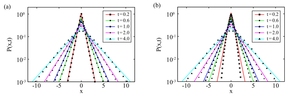
Figure 3: Short time diffusive properties of the EPK model Eq. (41). All model and simulation parameters are given in the text. Shown is the position probability density function $P(x,t)$ for the transition rates $\lambda=\{10,10^{2}\}$ (panels (b) and (a) respectively). Symbols correspond to the results of stochastic simulations at increasing values of time $t$ as given in the legends. Lines represent the Laplace distribution Eq. (45).

The asymptotic (long-term) behaviour of Eq. (41) corresponds to the Kac limit of Eq. (42). In this limit, $p_{\pm}(x,t,\beta)\simeq P(x,t)\,P^{\,\star}_{b}(\beta)/2$ and, following identical calculations developed in Giona et al. (2017a, c, d), one recovers the parabolic diffusion equation $\partial_{t}P(x,t)=D_{\rm eff}\,\partial_{x}^{2}P(x,t)$, with an effective diffusivity $D_{\rm eff}=D_{0}\,\langle\beta^{2}\rangle/(1-e^{-\kappa\,\beta_{\rm max}^{2}})$ where $\langle\beta^{2}\rangle=\int_{\mathcal{D}_{\beta}}\beta^{\prime\,2}\,P^{\,\star}_{b}(\beta^{\prime})\,\mathop{}\!\mathrm{d}\beta^{\prime}$. Correspondingly, the long-time asymptotics of Eq. (42) is expressed by the Gaussian heat kernel

$$P(x,t)=\frac{1}{\sqrt{4\,\pi\,D_{\rm eff}\,t}}\,\exp\left(-\frac{x^{2}}{4\,D_{\rm eff}\,t}\right)\>.$$ (46)

Figure 4 confirms these predictions numerically. The simulation protocol and model parameters used are the same as for Fig. 3. We only present the case $\lambda=10$, since the long-term asymptotic behaviour is the same for any value of $\lambda$. In this case, $D_{0}=1$, $\langle\beta^{2}\rangle=1$, so that $D_{\rm eff}=1$. In panel (a) the agreement between our prediction Eq. (46) and the simulation data is excellent. In panel (b) we show that the scaling of the mean square displacement $\sigma_{x}^{2}(t)$ is linear in time over all the time scales considered. We note that for finite $b_{max}$ a ballistic scaling for the mean square displacement $\sigma_{x}^{2}(t)\sim t^{2}$ for times $t\leq 1/\lambda$ is also observed due to the bounded propagation speed. This demonstrates that our model Eq. (41) can successfully reproduce Brownian yet non-Gaussian diffusive behaviour.

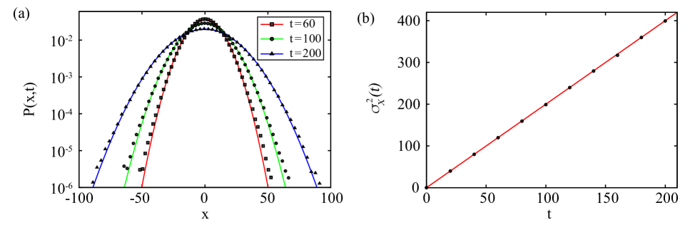
Figure 4: Long time diffusive properties of the EPK model Eq. (41). Here we consider only the transition rate $\lambda=10$, all the other model and simulation parameters are the same as in Fig. 3, see also the text. Symbols correspond to the results of stochastic simulations. (a) Position probability density function $P(x,t)$ at different times $t$ as given in the legend. Lines represent the Gaussian long time limit Eq. (46). (b) Mean square displacement $\sigma_{x}^{2}(t)$. The solid line corresponds to the Einsteinian scaling $\sigma_{x}^{2}(t)=2D_{\rm eff}\,t$, with $D_{\rm eff}=1$.

IV.3 Subdiffusive Lévy Walks

In their original formulation based on CTRWs, LWs have been shown to capture ballistic, normal and superdiffusive behaviour, according to the scaling properties of their transition time density distribution Zaburdaev et al. (2015). Other diffusional features, such as particularly subdiffusion, could only be achieved in a generalised version of LW dynamics, where a power-law kinematic relation between the displacement of the walker and the transition time was imposed Albers and Radons (2018a). We remark that the occurrence of long-term subdiffusive scaling in stochastic processes possessing finite propagation velocity has also already been obtained for symmetric random walks on fractals Ben-Avraham and Havlin (2000) or generalised PK processes in pre-fractal media Giona et al. (2016). Motivated by these results, in this section we show that we can formulate an EPK process that can capture short-term subdiffusion solely as the result of microscopic correlations among its transition rates.

We consider an EPK process where the transition rate of the Poissonian switching process $S$ is described by the stochastic process $\Lambda(t)$ attaining values in the bounded interval $\mathcal{D}_{\lambda}=[0,\lambda_{\rm max}]$. Specifically, we assume $\Lambda$ to generate a Markov chain dynamics, with transition rate $\mu(\lambda)$ and probability transition kernel $\mathcal{M}(\lambda,\lambda^{\prime})$ (see Appendix B). The corresponding extended PK process can then be defined as

$$\frac{dx(t)}{dt}=b\,(-1)^{\chi(t,\lambda(t))}\>.$$ (47)

The PPDW functions for this process, $p_{s}(x,t,\lambda)\equiv p(x,t,\lambda,s)$, are parametrised with respect to all the transitional parameters, here $s=\pm$ and $\lambda\in\mathcal{D}_{\lambda}$. The transitional parameters are transitionally independent as in the previous example. The temporal evolution equations can then be obtained similarly to Eq. (33), i.e.,

$$\frac{\partial p_{\pm}(x,t,\lambda)}{\partial t} =\mp b\,\frac{\partial p_{\pm}(x,t,\lambda)}{\partial x}\mp\lambda\,[p_{+}(x,t,\lambda)-p_{-}(x,t,\lambda)]-\mu(\lambda)\,p_{\pm}(x,t,\lambda)$$

$$\quad+\int_{0}^{\lambda_{\rm max}}\mu(\lambda^{\prime})\,\mathcal{M}(\lambda,\lambda^{\prime})\,p_{\pm}(x,t,\lambda^{\prime})\,\mathop{}\!\mathrm{d}\lambda^{\prime}\>.$$ (48)

Solutions of these equations are uniquely determined by the initial condition $p_{\pm}(x,\lambda,0)=p_{\pm}^{0}(x,\lambda)$.

First, we demonstrate that the process Eq. (47) generates a dynamic that shares the long-time statistical characteristics of the conventional LW. Let us assume $\mathcal{M}(\lambda,\lambda^{\prime})=\pi^{*}(\lambda)$, where $\pi^{*}(\lambda)$ is the equilibrium density function of the transition rate process. Under these assumptions, the transition time density for this process is given by

$$T(\tau)=\int_{\mathcal{D}_{\lambda}}\lambda\,e^{-\lambda\,\tau}\,\pi^{*}(\lambda)\,\mathop{}\!\mathrm{d}\lambda\>.$$ (49)

This equation follows by recalling that, once we fix $\lambda$, the time $\tau$ elapsed before the next transition is a random variable sampled from an exponential distribution with mean $\lambda$. We now specify the equilibrium density as

$$\pi^{*}(\lambda)=(1+\alpha)\,\lambda^{\alpha}$$ (50)

with $\alpha>-1$ and $\lambda_{max}=1$. In this case, $T(\tau)\sim\tau^{-(\alpha+2)}$ for large $\tau$. Therefore, this process reproduces qualitatively all the characteristic long-term diffusive features of the conventional LW as defined in Section II, provided we set $\xi=\alpha+1$. In particular, we can show that (i) for $-1<\alpha<0$ the process is ballistic, i.e., $\sigma_{x}^{2}(t)\sim t^{2}$; (ii) for $0<\alpha<1$ the process is superdiffusive, $\sigma_{x}^{2}(t)\sim t^{2-\alpha}$; and (iii) for $\alpha>1$, the process exhibits a linear Einsteinian scaling, $\sigma_{x}^{2}(t)\sim t$. Furthermore, we can show that (iv) the invariant function $p^{*}(z)=\sigma_{x}(t)\,P(x,t)|_{x=z\,\sigma_{x}(t)}$, with the probability density function for the process $P(x,t)=\int_{0}^{1}\left[p_{+}(x,t,\lambda)+p_{-}(x,t,\lambda)\right]\,\mathop{}\!\mathrm{d}\lambda$, is the same as that of the conventional LW. We verified all these results in numerical simulations; see Figs. 5(a) and (b) for some representative examples. We note that the different transition time densities for the process Eq. (47) and the LW Eq. (17) only affect their short-time statistical properties.

Remarkably, the formulation Eq. (47) of LW dynamics enables the explicit modelling of highly non-trivial transitional correlations through the full transition kernel $\mathcal{M}(\lambda,\lambda^{\prime})$. In particular, we assume that the transition rate process $\Lambda$ does not possess an invariant density. This is ensured by the condition

$$\int_{\mathcal{D}_{\lambda}}\lambda\,\mathcal{M}(\lambda,\lambda^{\prime})\,\mathop{}\!\mathrm{d}\lambda>\lambda^{\prime}\>.$$ (51)

In physical terms, this condition induces a progressive shift over time towards higher and higher values of the transition rate. As a specific example, we assume $\mathcal{M}(\lambda,\lambda^{\prime})=(\lambda^{\prime})^{\nu}/(a_{2}+a_{1})$ for $\lambda\in[\lambda^{\prime}-a_{1}/(\lambda^{\prime})^{\nu},\lambda^{\prime}+a_{2}/(\lambda^{\prime})^{\nu}]$ and zero otherwise, where $a_{1},\,a_{2}>0$ ($a_{2}>a_{1}$) and $\nu>0$ are constant. The shift is clearly determined by the fact that $\lambda$ at each transition is sampled uniformly from an asymmetric interval $[\lambda^{\prime}-c(\lambda^{\prime})a_{1},\lambda^{\prime}+c(\lambda^{\prime})a_{2}]$, where $c(\lambda^{\prime})=(\lambda^{\prime})^{-\nu}$ decreases progressively. This function is introduced to slow down the shift that would, otherwise, rapidly stop the motion. This shift towards higher values of $\lambda$ determines a progressive decrease of the local diffusivity, leading potentially to subdiffusive behaviour. This is verified in Fig. 5(c), where we plot $\sigma_{x}^{2}$ for this process obtained from numerical simulations. We run $10^{5}$ independent trajectories. Starting from a ballistic scaling for short times, as typical of all processes possessing finite propagation velocity, the mean square displacement for $t>10^{2}$ exhibits an anomalous long-time scaling with subdiffusive exponent $\gamma=0.8$. We note that this scaling is observed over more than four decades, $t\in[10^{2},10^{6}]$.

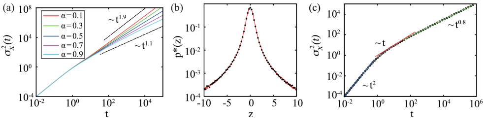
Figure 5: Statistical characterisation of the EPK model Eq. (48) for equilibrated transition rate dynamics (panels (a) and (b)) and for the general non-equilibrated case (panel (c)) (see main text for details). (a) Mean square displacement $\sigma_{x}^{2}(t)$ for $\alpha=\{0.1,\,0.3,\,0.5,\,0.7,\,0.9\}$, where $\alpha$ is the exponent of the power law determining the equilibrium density of the transition rates, see Eq. (50). Lines are generated by numerical simulations of the stochastic dynamic. Dashed lines indicate the scaling predictions for the extremal values of $\alpha$ in the range considered. (b) Invariant long time density $p^{*}(z)$ ($z=x/\sigma_{x}(t)$) at $\alpha=0.5$ (symbols), compared with the distribution of its corresponding LW (solid lines). (c) Mean square displacement $\sigma_{x}^{2}(t)$ for the same EPK model in non-equilibrated conditions. Three different diffusive regimes are indicated by straight lines. Markers represent the results of numerical simulations. Solid lines indicate the different scaling regimes exhibited by this dynamic.

V Conclusions and perspectives

Stochastic processes form a cornerstone of our mathematical description of physical reality. They enable the modelling of a wide variety of transport phenomena in the natural and social sciences, such as the random movements of cells, bacteria and viruses, the fluctuations of climate and the volatility of financial markets Bunde et al. (2018); Klages et al. (2008); Metzler and Klafter (2004). Typical stochastic models considered, however, fail to ensure finite velocities thus violating Einstein’s theory of special relativity. While these models still capture the correct statistics of motion on sufficiently long time scales, their representation of the real world is thus intrinsically defective. Partially they also lead to mathematical problems like diverging moments for the probability distributions of a random walker, with direct implications for physical observables obtained from such models. To solve this deep conceptual problem, stochastic processes with finite propagation speed have been introduced. Paradigmatic examples are PK processes Taylor (1921); Goldstein (1951); Kac (1974) and LWs Shlesinger et al. (1982); Geisel et al. (1985); Shlesinger and Klafter (1985); Klafter et al. (1987); Shlesinger et al. (1987); Geisel et al. (1988) yielding normal and anomalous diffusion, respectively. Despite their joint feature of finite propagation speeds, however, these two fundamental classes of stochastic processes have so far coexisted without exploring any cross-links between them.

Inspired by the novel formulation of LW dynamics proposed by Fedotov and collaborators Fedotov et al. (2015); Fedotov (2016), in this article we explored the connection between LWs and PK processes by showing that the latter models can be understood as a particular case of the former ones. Clarifying the relation between these two dynamics, by including Wiener processes as a special case, yielded our first main result. This is represented in Fig. 1 by the first three inner circles. In turn, this observation suggested the most natural stochastic differential equations describing LW path dynamics, Eqs. (16) and (17), which are obtained from suitably generalising the formalism of PK processes. This formulation neatly results from the definition of a LW process and, in this sense, greatly differs from other phenomenological models published in the literature that rely on subordination techniques Eule et al. (2012); Wang et al. (2019) or fractional derivatives Magdziarz et al. (2012), as the statistical characterization involves first-order evolution equations in time and space, whose mathematical structure resembles the linear Boltzmann equation Cercignani (1988). Owing to this analogy and to the analogy between the evolution equations for the partial densities and the mathematics of radiative transfer Chandrasekhar (1960), the mathematical approaches developed in these two fields can be consistently transferred to the study of EPK processes Cercignani (1988); Chandrasekhar (1960). With a reverse-engineering approach, we then used the cross-link between these processes to formulate a very general theoretical framework for stochastic models with finite propagation speed, which we called EPK theory. This theory contains LWs as a special case, as is depicted again in Fig. 1 by the fourth most outer circle. This is our second main result.

Motivated by experimental applications we then demonstrated by three explicit, practical examples the potential and the modelling power offered by our novel theory. We showed that EPK processes can capture senescing phenomena, where the mechanism for velocity changes depends explicitly on on the number of transitions occurred. From EPK theory we also obtained a microscopic interpretation of the intriguing and very actively explored transport phenomenon associated with Brownian yet non-Gaussian diffusion Wang et al. (2012a); Chechkin et al. (2017). Finally, we demonstrated that LWs may not only be superdiffusive but also subdiffusive, depending on more subtle microscopic details of the LW dynamic as captured by EPK theory. These novel diffusional features (anomalies) are ultimately obtained by exploiting the internal coupling between state variables and transitional parameters characteristic of EPK processes.

In this paper, we outlined the general framework of EPK theory in unbounded domains and in the absence of biasing fields (potential and/or pressure-driven velocity fields). The extension of our theory to transport problems in bounded settings can be achieved straightforwardly by applying the boundary conditions (absorbing, reflecting, or of mixed nature) already developed for hyperbolic transport problems involving PK processes and LWs Giona et al. (2016); Adrover et al. (2021); Giona et al. (2019a). The effects of external biasing fields can be included in two ways: The first one is to consider the EPK counterparts of the classical Ornstein-Uhlenbeck model, as discussed in Giona et al. (2017d) for simple PK processes. The second one is to consider the effect of the external potential on the transitional properties of the EPK model, by allowing for a dependence of the transition rates on the positional state variables. A number of important open problems and consequences still remain to be addressed, especially concerning the mathematical features of EPK models and their experimental applications.

From the perspective of stochastic theory, the first intriguing open problem is the formulation of a spectral theory of finite propagation speed processes (most notably LWs among them). We have preliminary evidence that the constraint imposed by the finite velocity may manifest itself as a lower bound in the real part of the spectrum. If confirmed, it would be interesting to investigate whether this is a universal property of all stochastic processes possessing finite propagation velocity. In this direction, a second top-priority problem is to develop a homogenisation theory for EPK processes. This is fundamental, as it could enable to calculate the hierarchy of moments and correlation functions associated with these stochastic processes. These are essential quantities to explore theoretically the ergodic and aging properties of a given class of stochastic processes. In addition, these results are also relevant from the perspective of experimental applications. Indeed, both moments and correlations are observables that can often be measured with great accuracy in experiments. Therefore, by comparing experimental data with model predictions of these observables, they could be employed to discern the most suitable finite propagation speed stochastic model for a given empirical diffusion dynamics. To complement this argument, our considerations further suggest that experimentalists should make an effort to measure the probability distribution of diffusive observables (such as position and/or velocity) with sufficiently large statistics to assess reliably the tails of these distributions. While stochastic processes with or without finite propagation speed might exhibit the same long-term asymptotic scaling of moments and/or correlations, the presence of ballistic peaks in the tails of these distributions is a hallmark that the diffusion observed empirically possesses finite velocities. Finally, while in this work we have focused on the single-particle case, another relevant research direction is the study of the emerging collective behaviour in ensembles of EPK particles potentially interacting among themselves. Along these lines, and by introducing persistence in terms of correlations, one may crosslink finite velocity stochastic theory with the very recent field of active matter Toner et al. (2005); Schweitzer (2007); Ramaswamy (2010); Vicsek and Zafeiris (2012); Marchetti et al. (2013). Given the additional biologically-motivated features that can be included in EPK theory, it will be interesting to systematically investigate what EPK models can further reproduce in terms of biologically significant dynamics.

We conclude by highlighting that EPK processes are not only of fundamental importance as models of transport phenomena, but also that they can be applied to basic and fundamental problems of statistical physics, providing a novel view of the latter. The boundedness of the transition rates characteristic of EPK processes allows to describe the dynamics of processes controlled by elementary events occurring at random transition times. This is the case of the quantum phenomenology associated with the interaction between molecules and photons. In this case, the elementary processes involve emission and absorption of energy quanta Einstein (1917). In this class falls also the stochastic representation of quantum systems interacting with an external environment H.-P. Breuer (2002). At sufficiently high (ambient) temperatures these processes can be described by a Poissonian statistics of the transition times Einstein (1917); H.-P. Breuer (2002). In the limit of very low temperatures, reachable e.g. by means of laser cooling techniques, the transitional statistics becomes more complex and correlated Bardou (2002) providing a natural application for EPK processes.

Another important field of application is the hydrodynamics of colloidal systems whenever particle/fluid interactions are accounted for in detail. Physically, this implies the transition from the Einstein-Langevin picture of Brownian motion (Stokes regime), to the realm where fluid inertia is no longer negligible (time-dependent Stokes regime) Stokes (1851); Landau (1959). These effects, originally discovered by Stokes in 1851 Stokes (1851), determine the occurrence of long-term power-law tails in the velocity autocorrelation functions, recently observed experimentally Jannasch et al. (2011); Franosch et al. (2011); Huang et al. (2011) for Brownian particles in a liquid. Preliminary results on a velocity-based representation of fluctuation-dissipation theorem indicates that EPK processes possessing a continuous velocity distribution, can be amongst the simplest candidate for representing the thermal/hydrodynamic fluctuations controlling Brownian and colloidal particle motion in inertial fluids both in the free space and in confined geometries.

Acknowledgements: RK thanks the TU Berlin and particularly his host, Prof. S.H.L.Klapp, for funding in the form of a Mercator Visiting Professorship, financed by the Deutsche Forschungsgemeinschaft (DFG, German Research Foundation) — Projektnummer 163436311 — SFB 910. He also acknowledges an External Fellowship from the London Mathematical Laboratory.

Appendix A Continuous-time random walks and their relation to Lévy walks

A one-dimensional continuous-time random walk is a stochastic process that describes the dynamic of a random walker on the real line that can wait for a random time $\tau$ at its current position before jumping over a random distance $\Delta$ either to the left or to the right. The pair of jump length and waiting time, $(\Delta,\tau)$, is sampled from a prescribed joint PDF $\phi(\Delta,\tau)$. The jump length distribution is $w(\Delta)=\int_{0}^{+\infty}\phi(\Delta,\tau)\mathop{}\!\mathrm{d}\tau$, where $\Delta\in\mathbb{R}$; likewise, the waiting time distribution is $T(\tau)=\int_{-\infty}^{+\infty}\phi(\Delta,\tau)\mathop{}\!\mathrm{d}\Delta$. Hence, a CTRW dynamic can be more naturally defined with respect to an operational time $n\in{\mathbb{N}}$, which simply counts the jump events occurred. The particle position $x_{n}$ at the physical time $t_{n}$ is then given by the equations of motion

$$x_{n+1} =x_{n}+\Delta_{n}\>, t_{n+1}=t_{n}+\tau_{n}\>,$$ (52)

with the pairs $(\Delta_{h},\tau_{h})$ and $(\Delta_{k},\tau_{k})$ being independent of each other for $h\neq k$. Traditionally, jump lengths and waiting times are further assumed to be independent, meaning that we can factorise the joint distribution as $\phi(\Delta,\tau)=w(\Delta)\,T(\tau)$. Under this assumption, the CTRW dynamic resembles that of the Wiener process Eq. (2) (which can be recovered in fact by assuming $w(\Delta)$ and $T(\tau)$ to be Gaussians Metzler and Klafter (2000)), in the sense that the walker can perform potentially unbounded random displacements depending on the prescribed jump length distribution $w(\Delta)$. This is manifest particularly in the Lévy flight model Mandelbrot (1982); Hughes et al. (1981); Shlesinger et al. (1995), where the probabilities of sampling very large displacements are enhanced by assuming a power law tailed jump length distribution.

In order to model a LW, we impose on Eqs. (52) the constraint of a finite and constant propagation speed $b$ Shlesinger et al. (1982); Geisel et al. (1985); Shlesinger and Klafter (1985); Klafter et al. (1987); Shlesinger et al. (1987); Geisel et al. (1988); Zumofen and Klafter (1993). This implies introducing a relation between $\Delta_{n}$ and $\tau_{n}$ in the form of

$$\Delta_{n}=s_{n}\,b\,\tau_{n},$$ (53)

where $s_{n}$ are random variables attaining values $\pm 1$ with equal probability. We highlight that this is not just a technicality, but it implies a complete change of perspective. Within this different interpretation, the waiting time $\tau$ in the original CTRW formulation becomes in the LW the transition time for a velocity change in one direction. In the special case of a two-state model the direction of motion is inverted at each transition event Zumofen and Klafter (1993), $\Delta_{n}=b\,s_{0}\,(-1)^{n}\,\tau_{n}$, where $s_{0}=\pm 1$ with equal probability determines the initial direction of motion.

Appendix B Poisson fields: definition and evolution equation

A $d$-dimensional Poisson field is a continuous stochastic process attaining values in a set, ${\mathcal{D}}_{\alpha}$, whose statistical description satisfies a continuous Markov chain dynamic defined by the transition rate function $\lambda(\boldsymbol{\alpha})\geq 0$, and by the transition probability kernel $A(\boldsymbol{\alpha},\boldsymbol{\alpha}^{\prime})$. The symbols $\boldsymbol{\alpha},\boldsymbol{\alpha}^{\prime}$ denote $d$-dimensional vectors in ${\mathcal{D}}_{\alpha}$. Let us now assume ${\mathcal{D}}_{\alpha}$ to be continuous. Thus, the probability $\mbox{Prob}[\{\boldsymbol{\Xi}(t)\in(\boldsymbol{\alpha},\boldsymbol{\alpha}+\mathop{}\!\mathrm{d}\boldsymbol{\alpha})\}]=\widehat{P}(\boldsymbol{\alpha},t)\,\mathop{}\!\mathrm{d}\boldsymbol{\alpha}$ ($\mathop{}\!\mathrm{d}\boldsymbol{\alpha}$ denotes a $d$-dimensional infinitesimal volume in $\mathcal{D}_{\alpha}$) is determined by the density function $\widehat{P}(\boldsymbol{\alpha},t)$ that satisfies the linear evolution equation

$$\frac{\partial\widehat{P}(\boldsymbol{\alpha},t)}{\partial t}=-\lambda(\boldsymbol{\alpha})\,\widehat{P}(\boldsymbol{\alpha},t)+\int_{{\mathcal{D}}_{\alpha}}\lambda(\boldsymbol{\alpha}^{\prime})\,A(\boldsymbol{\alpha},\boldsymbol{\alpha}^{\prime})\,\widehat{P}(\boldsymbol{\alpha}^{\prime},t)\,\mathop{}\!\mathrm{d}\boldsymbol{\alpha}^{\prime}\>.$$ (54)

The transition probability kernel $A(\boldsymbol{\alpha},\boldsymbol{\alpha}^{\prime})$ is a left stochastic kernel, i.e., $A(\boldsymbol{\alpha},\boldsymbol{\alpha}^{\prime})\geq 0$, $\int_{{\mathcal{D}}_{\alpha}}A(\boldsymbol{\alpha},\boldsymbol{\alpha}^{\prime})\,\mathop{}\!\mathrm{d}\boldsymbol{\alpha}=1$ for all $\boldsymbol{\alpha}^{\prime}\in{\mathcal{D}}_{\alpha}$. If ${\mathcal{D}}_{\alpha}$ is discrete instead, the statistical description of the Poisson field $\boldsymbol{\Xi}(t)$ is obtained directly in terms of the probability $\mathcal{P}(\boldsymbol{\alpha},t)=\mbox{Prob}[\{\boldsymbol{\Xi}(t)=\boldsymbol{\alpha}\in{\mathcal{D}}_{\alpha}\}]$, which satisfies an equation similar to Eq. (54) with the integral term substituted by the summation $\sum_{\boldsymbol{\alpha^{\prime}}\in{\mathcal{D}}_{\alpha}}\lambda(\boldsymbol{\alpha}^{\prime})\,A(\boldsymbol{\alpha},\boldsymbol{\alpha}^{\prime})\,\mathcal{P}(\boldsymbol{\alpha}^{\prime},t)$. Naturally, the condition on the transition kernel becomes $\sum_{\boldsymbol{\alpha}\in{\mathcal{D}}_{\alpha}}A(\boldsymbol{\alpha},\boldsymbol{\alpha}^{\prime})=1$ for every $\boldsymbol{\alpha}^{\prime}\in{\mathcal{D}}_{\alpha}$. We remark that any continuous Markov chain transition dynamic satisfies an equation similar to Eq. (54) with given rate and kernel functions.

Appendix C Lévy walks as specific overlapping Poisson-Kac processes

For a one-dimensional LW (see Subsec. II.3) our general framework boils down to $n=m=1$, ${\bf x}=x$, $\boldsymbol{\tau}=\tau$, and $\boldsymbol{\alpha}=\alpha$, which attains only the discrete values ${\mathcal{D}}_{\alpha}=\{\pm\}$. Moreover, ${\bf v}(x,\tau)=0$, $\lambda=\lambda(\tau)$, ${\bf w}(x,\tau)=1$ and ${\bf b}(x,\tau,\alpha)=\text{b}(\alpha)$, with $\text{b}(\pm)=\pm b$. Given the atomic nature of the transitional parameter $S(t)$, we can define

$$p(x,\tau,t,\alpha) = \sum_{s=\pm}p_{s}(x,\tau,t)\,\delta(\alpha-s)\>,$$ (55)

$$A(x,\tau,\alpha,\tau^{\prime},\alpha^{\prime}) = \sum_{s,q=\pm}\widehat{A}_{sq}(\tau,\tau^{\prime})\,\delta(\alpha-s)\,\delta(\alpha^{\prime}-q)\>,$$ (56)

in which the $2\times 2$ transition kernel $A$ does not depend on the state variable $x$. In order to recover a LW it is sufficient to consider the factorisation

$$\widehat{A}_{sq}(\tau,\tau^{\prime})=A_{sq}\,k(\tau,\tau^{\prime})\>,$$ (57)

where ${\bf A}=(A_{sq})_{s,q=\pm}$ is a left stochastic matrix and $k(\tau,\tau^{\prime})=\delta(\tau)$ (see Subsec. II.3). For the matrix ${\bf A}$, we consider the simplest form defining a two-state process, i.e.,

$${\bf A}=\left(\begin{array}[]{cc}0&1\\ 1&0\end{array}\right)\>.$$ (58)

Implementing all these simplifications in Eq. (31), we obtain the equations for the PPDW functions $p_{s}(x,\tau,t)$,

$$\frac{\partial p_{s}(x,\tau,t)}{\partial t}=-s\,b\,\frac{\partial p_{s}(x,\tau,t)}{\partial x}-\frac{\partial p_{s}(x,\tau,t)}{\partial\tau}-\lambda(\tau)\,p_{s}(x,\tau,t)+\delta(\tau)\,\int_{0}^{\infty}\lambda(\tau^{\prime})\,p_{\pi(s)}(x,\tau^{\prime},t)\,\mathop{}\!\mathrm{d}\tau^{\prime}\>,$$ (59)

where $\pi(s)$ represents the index flipping operation $\pi(\pm)=\mp$, which accounts for the structure of the Markovian transition matrix ${\bf A}$. For any $\tau>0$, the term $\propto\delta(\tau)$ is null, such that Eq. (59) reduces to the Eq. (8) previously derived for LW processes (see Subsec. II.3). The impulsive forcing term $\propto\delta(\tau)$ in Eq. (59) only affects the behaviour of $p_{s}(x,\tau,t)$ near $\tau=0$. The resolution of this impulsive discontinuity can be achieved by integrating Eq. (59) in the transitional age $\tau$ over an interval $[-\varepsilon,\varepsilon]$, with arbitrary $\varepsilon\rightarrow 0$. This interval contains $\tau=0$ as its internal point. In doing this, we are implicitly extending the domain of the PPDW functions $p_{s}(x,\tau,t)$ to negative $\tau$. Performing the integration, the $O(1)$-contributions stem solely from the convective term along the age-abscissa, $\partial p_{s}/\partial\tau$, and from the last impulsive recombination term $\propto\delta(\tau)$, while all other remaining terms are $O(\varepsilon)$. Thus, they are negligible in the limit $\epsilon\to 0$. In this way, Eq. (59) yields

$$-\int_{-\varepsilon}^{\varepsilon}\frac{\partial p_{s}(x,\tau,t)}{\partial\tau}\,\mathop{}\!\mathrm{d}\tau+\int_{0}^{\infty}\lambda(\tau^{\prime})\,p_{\pi(s)}(x,\tau^{\prime},t)\,\mathop{}\!\mathrm{d}\tau^{\prime}=0\>.$$ (60)

Since $\lim_{\varepsilon\rightarrow 0}p_{s}(x,\varepsilon,t)=p_{s}(x,0,t)$ and $\lim_{\varepsilon\rightarrow 0^{+}}p_{s}(x,-\varepsilon,t)=0$, Eq. (60) reduces to the boundary condition Eq. (11). In point of fact, Eq. (59) represents in a compact form both the evolution equations (8) and the age boundary condition (11). This equation possesses the typical integro-differential structure of a generalised PK process in the presence of an impulsive recombination in $\tau$, in which the dynamics for $\tau\in(0,\infty)$ gives rise to Eqs. (8), whereas the impulsive discontinuity at $\tau=0$ can be resolved by the boundary condition Eq. (11).

We highlight that within our generalised theory LWs can be defined straightforwardly in higher spatial dimensions. In contrast, only few models in two spatial dimensions with ad hoc assumptions on the transitional dynamics have been obtained by using the conventional formalism of CTRWs Zaburdaev et al. (2016a). As a matter of fact, all these models can be naturally recovered as special cases of our Eq. (31), as follows: First, in the product model, we assume that the random walker performs completely independent one-dimensional LWs in both the $x$- and $y$-direction. Therefore, within our formalism, the PPDW functions can be factorised as $p(\textbf{x},\boldsymbol{\tau},t,\boldsymbol{\alpha})=p(x,\tau_{x},t,\alpha_{x})p(y,\tau_{y},t,\alpha_{y})$, where we introduced transitional age variables $\tau_{x}$ and $\tau_{y}$, and independent stochastic parametrisations $\alpha_{x}$ and $\alpha_{y}$ in each direction. If we assume that all other characteristic parameters of these processes are the same as those of the one-dimensional LW discussed above, each PPDW functions then satisfy the same Eq. (59) in its corresponding spatial direction. Second, in the XY model, we assume that the random walker can only move along the x- or y-axis in either direction. In this case, we therefore set $\boldsymbol{\tau}=\tau$, $\boldsymbol{\alpha}=\alpha$ with $\mathcal{D}_{\alpha}=\{0,1,2,3\}$, and $\textbf{b}(\textbf{x},\tau,\alpha)=\textbf{b}(\alpha)=b(\cos{(\alpha\pi/2)},\sin{(\alpha\pi/2)})$. As the stochastic parameter can only attain discrete values, we can make assumptions similar to Eq. (56) and (57) with the only difference being in the definition of the Markovian transitional matrix; in this case, this is defined as

$${\bf A}=\frac{1}{3}\left(\begin{array}[]{cccc}0&1&1&1\\ 1&0&1&1\\ 1&1&0&1\\ 1&1&1&0\end{array}\right)\>.$$ (61)

Finally, in the uniform model, we assume that the random walker at each transition can choose any random new direction. We therefore set $\boldsymbol{\tau}=\tau$, $\boldsymbol{\alpha}=\alpha$ with $\mathcal{D}_{\alpha}=[0,2\pi)$, and $\textbf{b}(\textbf{x},\tau,\alpha)=\textbf{b}(\alpha)=b(\cos{(\alpha)},\sin{(\alpha)})$. As the stochastic parameter here attains values in a continuous set, Eq. (31) applies directly with the transitional matrix

$$A(\textbf{x},\alpha,\tau,\alpha^{\prime},\tau^{\prime})=\frac{\delta(\tau)}{2\pi}.$$ (62)

References

- Bunde et al. (2018) A. Bunde, J. Caro, J. Kaerger, and G. Vogl, eds., Diffusive Spreading in Nature, Technology and Society (Springer, Berlin, 2018).
- van Kampen (1992) N. van Kampen, Stochastic processes in physics and chemistry (North Holland, Amsterdam, 1992).
- Risken (1996) H. Risken, The Fokker-Planck Equation, 2nd ed. (Springer, Berlin, 1996).
- Gardiner (2009) C. Gardiner, Stochastic Methods: A Handbook for the Natural and Social Sciences, 4th ed. (Springer, Berlin, 2009).
- Zwanzig (2001) R. Zwanzig, Nonequilibrium statistical mechanics (Oxford University Press, Oxford, 2001).
- Langevin (1908) P. Langevin, “Sur la théorie du mouvement Brownien,” C.R. Acad. Sci. (Paris) 146, 530–533 (1908), see also the English translation in Am. J. Phys. 65, 1079 (1997).
- Coffey et al. (2004) W. Coffey, Y. P. Kalmykov, and J. T. Waldron, The Langevin Equation (World Scientific, Singapore, 2004).
- Gnedenko and Kolmogorov (1954) B. V. Gnedenko and A. N. Kolmogorov, Limit distributions for sums of independent random variables (Addison-Wesley, Cambridge, United States, 1954).
- Cattaneo (1948) C. Cattaneo, “Sulla conduzione del calore,” Atti Semin. Mat. Fis. Univ. Modena 3, 83–101 (1948).
- Dunkel and Hänggi (2009) J. Dunkel and P. Hänggi, “Relativistic Brownian motion,” Phys. Rep. 471, 1 – 73 (2009).
- Rezzolla and Zanotti (2013) L. Rezzolla and O. Zanotti, Relativistic Hydrodynamics (Oxford University Press, Oxford, 2013).
- Blum et al. (2006) J. Blum, S. Bruns, D. Rademacher, A. Voss, B. Willenberg, and M. Krause, “Measurement of the translational and rotational Brownian motion of individual particles in a rarefied gas,” Phys. Rev. Lett. 97, 230601 (2006).
- Yoo et al. (1990) K. M. Yoo, Feng Liu, and R. R. Alfano, “When does the diffusion approximation fail to describe photon transport in random media?” Phys. Rev. Lett. 64, 2647–2650 (1990).
- Chang et al. (2008) C. W. Chang, D. Okawa, H. Garcia, A. Majumdar, and A. Zettl, “Breakdown of Fourier’s law in nanotube thermal conductors,” Phys. Rev. Lett. 101, 075903 (2008).
- Sellitto et al. (2016) A. Sellitto, V. A. Cimmelli, and D. Jou, Mesoscopic Theories of Heat Transport in Nanosystems (Springer, Berlin, 2016).
- Joseph and Preziosi (1989) D. D. Joseph and L. Preziosi, “Heat waves,” Rev. Mod. Phys. 61, 41–73 (1989).
- Metzler and Klafter (2000) R. Metzler and J. Klafter, “The random walk’s guide to anomalous diffusion: A fractional dynamics approach,” Phys. Rep. 339, 1–77 (2000).
- Klages et al. (2008) R. Klages, G. Radons, and I. M. Sokolov, eds., Anomalous transport: Foundations and Applications (Wiley-VCH, Berlin, 2008).
- Shlesinger et al. (1993) M. F. Shlesinger, G. M. Zaslavsky, and J. Klafter, “Strange kinetics,” Nature 363, 31–37 (1993).
- Klafter et al. (1996) J. Klafter, M. F. Shlesinger, and G. Zumofen, “Beyond Brownian motion,” Phys. Today 49, 33–39 (1996).
- Metzler et al. (2014) R. Metzler, J.-H. J., A. G. Cherstvy, and E. Barkai, “Anomalous diffusion models and their properties: non-stationarity, non-ergodicity, and ageing at the centenary of single particle tracking,” Phys. Chem. Chem. Phys. 16, 24128–24164 (2014).
- Zaburdaev et al. (2015) V. Zaburdaev, S. Denisov, and J. Klafter, “Lévy walks,” Rev. Mod. Phys. 87, 483–529 (2015).
- Metzler and Klafter (2004) R. Metzler and J. Klafter, “The restaurant at the end of the random walk: Recent developments in the description of anomalous transport by fractional dynamics,” J. Phys. A: Math. Gen. 37, R161–R208 (2004).
- Viswanathan et al. (2011) G. M Viswanathan, M. G. E. da Luz, E. P. Raposo, and H. E. Stanley, The physics of foraging (Cambridge University Press, Cambridge, 2011).
- Mandelbrot (1982) B. B. Mandelbrot, The fractal geometry of nature (W.H. Freeman and Company, San Francisco, 1982).
- Klages (2016) R. Klages, “Search for food of birds, fish and insects,” (2016), book chapter in: A.Bunde, J.Caro, J.Kaerger, G.Vogl (Eds.), Diffusive Spreading in Nature, Technology and Society. (Springer, Berlin).
- Shlesinger et al. (1982) M. F. Shlesinger, J. Klafter, and Y. M. Wong, “Random walks with infinite spatial and temporal moments,” J. Stat. Phys. 27, 499–512 (1982).
- Geisel et al. (1985) T. Geisel, J. Nierwetberg, and A. Zacherl, “Accelerated diffusion in Josephson junctions and related chaotic systems,” Phys. Rev. Lett. 54, 616–619 (1985).
- Shlesinger and Klafter (1985) M. F. Shlesinger and J. Klafter, “Accelerated diffusion in Josephson-junctions and related chaotic systems - comment,” Phys. Rev. Lett. 54, 2551 (1985).
- Klafter et al. (1987) J. Klafter, A. Blumen, and M. F. Shlesinger, “Stochastic pathway to anomalous diffusion,” Phys. Rev. A 35, 3081–3085 (1987).
- Shlesinger et al. (1987) M. F. Shlesinger, B. J. West, and J. Klafter, “Lévy dynamics of enhanced diffusion: Application to turbulence,” Phys. Rev. Lett. 58, 1100–1103 (1987).
- Geisel et al. (1988) T. Geisel, A. Zacherl, and G. Radons, “Chaotic diffusion and 1/f-noise of particles in two-dimensional solids,” Z. Phys. B 71, 117–127 (1988).
- Zumofen and Klafter (1993) G. Zumofen and J. Klafter, “Scale-invariant motion in intermittent chaotic systems,” Phys. Rev. E 47, 851–863 (1993).
- Shlesinger (1979) M. F. Shlesinger, “Correlation effects on frequency dependent conductivity: application to superionic conductors,” Solid State Commun. 32, 1207–1210 (1979).
- Becker-Kern et al. (2004) P. Becker-Kern, M. M. Meerschaert, and H. -P. Scheffler, “Limit theorems for coupled continuous time random walks,” Ann. Prob. 32, 730–756 (2004).
- Rebenshtok et al. (2014) A. Rebenshtok, S. Denisov, P. Hänggi, and E. Barkai, “Non-normalizable densities in strong anomalous diffusion: Beyond the central limit theorem,” Phys. Rev. Lett. 112, 110601 (2014).
- Fedotov (2016) S. Fedotov, “Single integrodifferential wave equation for a Lévy walk,” Phys. Rev. E 93, 020101 (2016).
- Magdziarz and Zorawik (2016) M. Magdziarz and T. Zorawik, “Explicit densities of multidimensional ballistic Lévy walks,” Phys. Rev. E 94, 022130 (2016).
- Palyulin et al. (2019) V. V. Palyulin, G. Blackburn, M. A. Lomholt, N. W. Watkins, R. Metzler, R. Klages, and A. V. Chechkin, “First passage and first hitting times of Lévy flights and Lévy walks,” New J. Phys. 21, 103028 (2019).
- Reynolds (2018) A. M. Reynolds, “Current status and future directions of Lévy walk research,” Biol. Open 7, 03016 (2018).
- Taylor (1921) G. I. Taylor, “Diffusion by continuous movements,” Proc. London Math Soc. 20, 196–212 (1921).
- Goldstein (1951) S. Goldstein, “On diffusion by discontinuous movements, and on the telegraph equation,” Q. J. Mech. Appl. Math. 4, 129–156 (1951).
- Kac (1974) M. Kac, “A stochastic model related to the telegrapher’s equation,” Rocky Mount. J. Math. 4, 497–509 (1974).
- Note (1) We note that any attempt to extend this equation to higher spatial dimensions fails to ensure the positivity of the corresponding PDF Körner and Bergmann (1998); Giona et al. (2017a).
- Cattaneo (1958) C. Cattaneo, “Sur une forme de l’equation de la chaleur eliminant le paradoxe d’une propagation instantanee,” C. R. Acad. Sc. Paris 247, 431–433 (1958).
- Bena (2006) I. Bena, “Dichotomous Markov noise: exact results for out-of-equilibrium systems,” Int. J. Mod. Phys. B 20, 2825–2888 (2006).
- Weiss (2007) G. H. Weiss, “Some applications of persistent random walks and the telegrapher ’ s equation,” Physica A 311, 381–410 (2007).
- Kolesnik (2008) A. D. Kolesnik, “Random motions at finite speed in higher dimensions,” J. Stat. Phys. 131, 1039–1065 (2008).
- Kolesnik and Pinsky (2011) A. D. Kolesnik and M. A. Pinsky, “Random evolutions are driven by the hyperparabolic operators,” J. Stat. Phys. 142, 828–846 (2011).
- Gaveau et al. (1984) B. Gaveau, T. Jacobson, M. Kac, and L. S. Schulman, “Relativistic extension of the analogy between quantum mechanics and Brownian motion,” Phys. Rev. Lett. 53, 419–422 (1984).
- Rosenau (1993) P. Rosenau, “Random walker and the telegrapher’s equation: A paradigm of a generalized hydrodynamics,” Phys. Rev. E 48, R655–R657 (1993).
- Müller and Ruggeri (1993) I. Müller and T. Ruggeri, Extended Thermodynamics (Springer, New York, 1993).
- Giona et al. (2017a) M. Giona, A. Brasiello, and S. Crescitelli, “Stochastic foundations of undulatory transport phenomena: generalized Poisson-Kac processes — part i basic theory,” J. Phys. A: Math. Theor. 50, 335002/1–43 (2017a).
- Giona (2017) M. Giona, “Variational principles and Lagrangian functions for stochastic processes and their dissipative statistical descriptions,” Physica A 473, 561–577 (2017).
- Giona et al. (2017b) M. Giona, A. Brasiello, and S. Crescitelli, “Kac limit and thermodynamic characterization of stochastic dynamics driven by Poisson-Kac fluctuations,” Eur. Phys. J. Spec. Top. 226, 2299–2310 (2017b).
- Einstein (1917) A. Einstein, “Zur Quantentheorie der Strahlung,” Phys. Zeitschrift 18, 121–128 (1917).
- H.-P. Breuer (2002) H. -P. Breuer, and F. Petruccione, The theory of open quantum systems (Clarendon Press, Oxford, 2002).
- Weiss (1994) G. H. Weiss, Aspects and applications of the random walk (North-Holland, Amsterdam, 1994).
- Giona (2018) M. Giona, “Lattice random walk: an old problem with a future ahead,” Phys. Scr. 93, 095201 (2018).
- Fedotov et al. (2015) S. Fedotov, A. Tan, and A. Zubarev, “Persistent random walk of cells involving anomalous effects and random death,” Phys. Rev. E 91, 1–10 (2015).
- Giona et al. (2019a) M. Giona, M. D’Ovidio, Davide Cocco, A. Cairoli, and R. Klages, “Age representation of Lévy walks: partial density waves, relaxation and first passage time statistics,” J. Phys. A 52, 384001 (2019a).
- Chen et al. (2015) K. Chen, B. Wang, and S. Granick, “Memoryless self-reinforcing directionality in endosomal active transport within living cells,” Nat. Mater. 14, 589–593 (2015).
- Song et al. (2018) M. S. Song, H. C. Moon, J. H. Jeon, and H. Y. Park, “Neuronal messenger ribonucleoprotein transport follows an aging Lévy walk,” Nat. Commun. 9, 1–8 (2018).
- Korabel et al. (2018) N. Korabel, T. A. Waigh, S. Fedotov, and V. J. Allan, “Non-Markovian intracellular transport with sub-diffusion and run-length dependent detachment rate,” PLoS ONE 13, e0207436/1–23 (2018).
- Wang et al. (2012a) B. Wang, J. Kuo, S. C. Bae, and S. Granick, “When Brownian diffusion is not Gaussian,” Nature Mater. 11, 481–485 (2012a).
- Chechkin et al. (2017) A. V. Chechkin, F. Seno, R. Metzler, and I. M. Sokolov, “Brownian yet non-Gaussian diffusion: From superstatistics to subordination of diffusing diffusivities,” Phys. Rev. X 7, 021002 (2017).
- Pinsky (1991) M. A Pinsky, Lectures on Random Evolution (World Scientific, Singapore, 1991).
- Zaburdaev et al. (2016a) V. Zaburdaev, I. Fouxon, S. Denisov, and E. Barkai, “Superdiffusive dispersals impart the geometry of underlying random walks,” Phys. Rev. Lett. 117, 270601 (2016a).
- Albers and Radons (2018a) T. Albers and G. Radons, “Exact results for the nonergodicity of -dimensional generalized Lévy walks,” Phys. Rev. Lett. 120, 104501 (2018a).
- Note (2) Without loss of generality, we restrict ourselves here and in the following to two-state LWs. We remark, however, that the velocity LW model could easily be embedded into our general theory that we develop here by appropriately adjusting the transition matrix Eq. (58) in Appendix C.
- Hughes et al. (1981) B. D. Hughes, M. F. Shlesinger, and E. W. Montroll, “Random walks with self-similar clusters,” Proc. Natl. Acad. Sci. 78, 3287–3291 (1981).
- Shlesinger et al. (1995) M. F. Shlesinger, G. M. Zaslavsky, and U. Frisch, Lévy flights and related topics in Physics, Lecture notes in Physics, Vol. 450 (Springer-Verlag, 1995).
- Sokolov and Metzler (2003) I. M. Sokolov and R. Metzler, “Towards deterministic equations for Lévy walks: The fractional material derivative,” Phys. Rev. E 67, 010101 (2003).
- Friedrich et al. (2006) R. Friedrich, F. Jenko, A. Baule, and S. Eule, “Anomalous Diffusion of Inertial, Weakly Damped Particles,” Phys. Rev. Lett. 96, 230601 (2006).
- Cairoli and Baule (2015) A. Cairoli and A. Baule, “Anomalous Processes with General Waiting Times: Functionals and Multipoint Structure,” Phys. Rev. Lett. 115, 110601 (2015).
- Campos et al. (2015) D. Campos, E. Abad, V. Méndez, S. B. Yuste, and K. Lindenberg, “Optimal search strategies of space-time coupled random walkers with finite lifetimes,” Phys. Rev. E 91, 052115 (2015).
- Cox and Miller (1965) D. R. Cox and H. D. Miller, The theory of stochastic processes (Methuen, London, 1965).
- Lee and Wang (2003) E. T. Lee and J. Wang, Statistical methods for survival data analysis, Vol. 476 (John Wiley & Sons, 2003).
-
Note (3)
To be complete, we need also to supplement the model with
regularity conditions at infinity with respect to both and .
Specifically, we assume that ,