Learning Thermodynamically Stable and Galilean Invariant Partial Differential Equations for Non-equilibrium Flows
Juntao Huang 111Department of Mathematics, Michigan State University, East Lansing, MI 48824, USA. Zhiting Ma 222Department of Mathematical Sciences, Tsinghua University, Beijing, China. Yizhou Zhou 22footnotemark: 2 Wen-An Yong 22footnotemark: 2, ‡‡‡E-mail: wayong@tsinghua.edu.cn. Corresponding author
Abstract
In this work, we develop a method for learning interpretable, thermodynamically stable and Galilean invariant partial differential equations (PDEs) based on the Conservation-dissipation Formalism of irreversible thermodynamics. As governing equations for non-equilibrium flows in one dimension, the learned PDEs are parameterized by fully-connected neural networks and satisfy the conservation-dissipation principle automatically. In particular, they are hyperbolic balance laws and Galilean invariant. The training data are generated from a kinetic model with smooth initial data. Numerical results indicate that the learned PDEs can achieve good accuracy in a wide range of Knudsen numbers. Remarkably, the learned dynamics can give satisfactory results with randomly sampled discontinuous initial data and Sod’s shock tube problem although it is trained only with smooth initial data.
Key Words: Machine learning; Non-equilibrium thermodynamics; Conservation-dissipation formalism; Hyperbolic balance laws; Kinetic equation; Galilean invariance.
1 Introduction
Emergence of machine learning and data science has brought new vitality to the development of various scientific disciplines. Mostly, such disciplines are based on certain fundamental principles which can be described with mathematical frameworks. The frameworks usually contain problem-dependent freedoms. Besides the traditional approaches like experiments, machine learning is a promising alternative in fixing the freedoms. In this sense, the booming data-based technique can display its power by a proper combination with reliable scientific theories.
Thermodynamics is a classical theory studying relationships among various apparently unrelated variables or parameters characterizing a thermodynamic system. For non-equilibrium systems, it was explained in [41] that the most natural form of the expected relations are evolution partial differential equations (PDEs). Thus, the core task of irreversible thermodynamics is choosing suitable variables and determining their evolution equations. However, no well-accepted rules have been given so far and consequently there are many different schools, such as Classical Irreversible Thermodynamics [10], Rational Extended Thermodynamics [27], Extended Irreversible Thermodynamics [20, 22], General Equation for Non-equilibrium Reversible–irreversible Coupling [29, 30], Conservation-dissipation Formalism (CDF) [47], Energetic Variational Approach [17], and so on. An exposition of different versions of thermodynamics can be found in [28] and references cited therein.
This project focuses on a combination of machine learning with the CDF theory mentioned above. CDF is based on the first and second laws of thermodynamics. It assumes that certain conservation laws are known a priori. By postulating the existence of an entropy function and a dissipative matrix, we follow a Conservation-dissipation Principle distilled in [40] to choose the non-equilibrium variables and derive the corresponding evolution equations. The PDEs thus obtained are hyperbolic balance laws (first-order PDEs) which naturally meet four fundamental physical requirements proposed in [41]: the observability of physical phenomena, time-irreversibility, long-time tendency to equilibrium, and compatibility with existing classical theories. The importance of these requirements were expounded in [41]. In CDF, the entropy function and dissipative matrix are problem-dependent and constitute its freedoms. These freedoms can be fixed by resorting to machine learning. Once the freedoms are determined, we obtain interpretable and thermodynamically stable PDEs governing the thermodynamic system under consideration.
As a start of this project, the present paper is devoted to finding the governing macroscopic equations for one-dimensional non-equilibrium flows. To be specific, we assume that the flow obeys the mesoscopic BGK (Bhatnagar-Gross-Krook) equation in kinetic theory. Thus, the classical conservation laws of mass, momentum and energy are known a priori. By adding one more (non-equilibrium) variable, we obtain a hyperbolic system of first-order PDEs with four unknown variables, which is Galilean invariant. Then we use fully connected neural networks to represent the entropy function and dissipation matrix. The training data are generated by numerically solving the BGK model with smooth initial data. The neural network representations for the hidden dynamics are trained by minimizing a loss function based on a discrete version of the CDF-based PDEs acting on the training data.
Numerical results show that our CDF-based machine learning model indeed satisfies the conservation-dissipation principle. This particularly implies that the learned PDEs are symmetrizable hyperbolic. Moreover, the model can achieve good accuracy in a wide range of Knudsen numbers for both randomly sampled smooth and discontinuous initial data. In particular, its performance on Sod’s shock tube problem [35] is better than the Euler equations in both hydrodynamic and kinetic regimes. Remarkably, the learned dynamics can give satisfactory results with discontinuous initial data although it is trained only with smooth initial data.
The macroscopic governing equations obtained above can also be understood as a moment closure system of the BGK model. However, it is important to point out that the CDF does not necessarily rely on the kinetic theory. Here we use the kinetic model just because we have no other means to obtain the training data. We are expecting to have such data from experiments or other means so that the CDF framework can exhibit its potential in a wide range of problems. In addition, note that the CDF theory itself allows more non-equilibrium variables. Here we choose only one non-equilibrium variable merely for the sake of simplicity. It is possible to achieve better results by adding more non-equilibrium variables.
As to the moment closure system, we mention the recent work [14], where the authors introduced a framework to construct interpretable moment closure models for kinetic problems. They firstly learned a set of generalized moments using the auto-encoder to optimally represent the underlying velocity distribution, and then learned the moment closure model for the generalized moments using neural networks with the aim of best capturing the associated dynamics of the kinetic equation. In this way, some novel moment closure systems are obtained and give good prediction results. Nevertheless, it is not clear whether the moment closure systems obtained in [14] are hyperbolic or preserve the dissipation property of the kinetic equation characterized by the H-theorem. In contrast, the hyperbolicity and dissipation property are enforced in our CDF-based PDEs automatically.
Other recent works on learning PDEs have the following. In [24], the authors designed a neural network with Galilean invariance to discover the Reynolds stress anisotropy tensor in turbulence models from high-fidelity simulation data. In [23], a neural network which preserves the rotational symmetry was constructed to approximate the constitutive laws in non-Newtonian fluid models. In [31, 32], by resorting to the Gaussian process regression or neural networks named Physics-Informed Neural Networks, some classical PDEs with unknown parameters or functions are explored. This was further applied in many realistic problems [8, 43, 39]. In [4, 34], a data-based method called SINDy (Sparse Identification of Nonlinear Dynamics) was developed to discover dynamical systems from the perspective of sparse regression and compressed sensing. In [26, 25], the authors used a symbolic neural network called PDE-Net to uncover the analytic form of PDEs.
There are more works about learning ordinary differential equations (ODEs). For Hamiltonian systems in classical mechanics, different neural networks such as SympNets and HénonNet have been designed in [19, 5]. More works on learning Hamiltonian systems can be found in [13, 37, 46] and references cited therein. In [21], ODEs with dissipation structure are considered and the dissipation structure was built into the neural network by jointly learning the dynamic model and a Lyapunov function. In a very recent work [42], a generalized Onsager principle was proposed and a so-called OnsagerNet was designed. In a series of works [15, 44, 38, 45], deep neural networks with symmetry-preserving property are explored to present the potential energy surface (PES) that describes the interaction between all the nuclei in the system in the molecular dynamics. For more details of the development of the physics-based modeling with machine learning, we refer readers to the review paper [16].
The paper is organized as follows. The general CDF theory is briefly reviewed in Section 2. In Section 3, we construct a simple CDF-based model for non-equilibrium flows. Section 4 is devoted to a detailed procedure to learn the freedoms in the model. The effectiveness of the procedure is demonstrated through numerical results in Section 5. Some concluding remarks are given in Section 6.
2 Preliminaries
In this section, we briefly review the CDF theory [47]. It is concerned with an irreversible process which obeys some conservation laws of the form
| (2.1) |
Here represents conserved variables depending on the time and spatial coordinates , with the dimension of space, and is the corresponding flux along the -direction. If each is given in terms of the conserved variables, the system (2.1) becomes closed. In this case, the system is considered to be in local equilibrium and is also referred to as equilibrium variables. However, very often depends on some extra variables in addition to the conserved ones. The extra variables characterize non-equilibrium features of the system under consideration, called non-equilibrium or dissipative variables, and their choice is not unique.
Motivated by the Extended Thermodynamics [27, 20], in CDF we choose a set of dissipative variables so that the flux in (2.1) can be expressed as and seek evolution equations of in the form
| (2.2) |
This is our constitutive equation. Here is the corresponding flux and is the source vanishing at equilibrium. Together with the conservation laws (2.1), the evolution of the non-equilibrium system is governed by first-order PDEs
| (2.3) |
where
It was observed in [40] that many classical PDEs of the form (2.3) respect the following so-called Conservation-dissipation Principle:
-
(i)
There is a strictly concave smooth function , called entropy (density), such that the matrix product is symmetric for each and for all under consideration.
-
(ii)
There is a positive definite matrix , called dissipation matrix, such that the non-zero source can be written as .
Here the subscript stands for the corresponding partial derivative, for instance and , and should be understood as a column vector. Note that the dissipation matrix is not assumed to be symmetric, and its positive definiteness means that of the symmetric part .
Inspired by the above observation, we try to determine the constitutive relation (2.2) so that the resultant balance laws (2.3) also respect the conservation-dissipation principle (see an example in the next section). This is our Conservation-dissipation Formalism (CDF) proposed in [47].
This formalism has two freedoms: the entropy function and the dissipation matrix . They are both functions of the state variable . The former is strictly concave and the latter is positive definite. Except these, no further restriction is imposed on the freedoms. Specific expressions of and should be problem-dependent. With these freedoms, CDF provides a tailored platform for machine learning to display its power.
On the conservation-dissipation principle, we make the following simple comments. Condition (i) is the well-known entropy condition for hyperbolic conservation laws [11, 12]. It ensures that the first-order system (2.3) is globally symmetrizable hyperbolic and thereby well-posed [9]. Condition (ii) is a nonlinearization of the celebrated Onsager reciprocal relation for scalar irreversible processes [10]. Together with the first condition, it can be regarded as a stability criterion for non-equilibrium thermodynamics. As shown in [41], this criterion guarantees that the CDF-based PDEs reflect the observability of physical phenomena, time-irreversibility, long-time tendency to equilibrium, and compatibility with existing classical theories. Further comments can be founded in [41].
3 A CDF-based model
Consider an electrically neutral fluid without external forces. Its motion obeys the conservation laws of mass, momentum and energy [20]:
| (3.1) | ||||
Here is the fluid density, is the velocity, is the total energy with the specific internal energy, is the pressure tensor, and represents the heat flux. This system gives the evolution of variables . It is closed only if and are specified. In [47], the CDF was used to obtain a set of evolution equations for these variables with the two freedoms— the corresponding entropy function and the dissipation matrix.
The goal of this paper is to fix the freedoms with machine learning. For simplicity, we only consider the one-dimensional problem. Moreover, in order to have reasonable training data, we turn to the one-dimensional BGK model
| (3.2) |
meaning that the fluid flow is governed by this kinetic model. Here is a distribution function with the particle velocity, is the dimensionless Knudsen number, and is the Maxwellian
with
| (3.3) |
It is well-known that the one-dimensional BGK model implies the conservation laws (3.1) with the pressure tensor becoming a scalar , ,
| (3.4) |
In fact, multiplying (3.2) with and integrating the resultant equations over will immediately lead to the conservation laws (3.1) (see e.g. [36]). Notice that for the one-dimensional kinetic model, we have the following equation of state . Thus, only the heat flux in (3.1) is an extra variable.
To close (3.1) with CDF, we firstly recall that the system in equilibrium has a specific entropy [36]
where is the Boltzmann constant, is the specific volume, and is a constant. Clearly, this entropy function is concave with respect to . In what follows, we take for simplicity.
Furthermore, we introduce a new dissipative variable and postulate that a specific entropy of the form
exists for the non-equilibrium system under consideration. Here for simplicity we have assumed that there is no cross-terms between and . According to the conservation-dissipation principle, the undetermined and non-equilibrium part should be a concave function of with the Knudsen number as a parameter. For such a concave function , it is well-known that the function defined as
can act as the entropy in the conservation-dissipation principle. Namely, it is strictly concave with respect to .
Next we follow [47] and introduce the differential operator acting on a function as . Using the conservation laws (3.1), we calculate
with . Here we have used and . This calculation suggests that is the entropy flux and is the entropy production.
According to the calculation above, we choose the heat flux
and the evolution equation for as
with a positive function. Here is independent of the velocity such that the model is Galilean invariant. By such a choice, we have the entropy production
Moreover, we notice that the non-equilibrium variable can be globally expressed in terms of and due to the strict concavity of with respect to .
Consequently, we arrive at the following balance laws
| (3.5) | ||||
with the freedoms and . Here we notice that the temperature for the one-dimensional kinetic model. This system satisfies the conservation-dissipation principle and thereby is globally symmetrizable hyperbolic. Moreover, it is Galilean invariant.
4 Learning the freedoms
In this section, we present a procedure to learn the two undetermined functions and in (3.5). Note that an unlimited amount of training data can be obtained by numerically solving the BGK model and then by computing the moments in (3.3)-(3.4). The details are given in Section 5.
Although the training data are available, the values of cannot be obtained directly since has not been fixed yet. Therefore, we use the variables with and rewrite the balance laws (3.5) as
| (4.1) | ||||
with
For smooth solutions, the system (4.1) is equivalent to the balance laws (3.5). Recall that the non-equilibrium variable can be globally expressed in terms of and due to the strict concavity of with respect to . Then can be viewed as a function of . Therefore, our task becomes to learn the negative and the positive .
Because the training data are known only at discrete space-time points, it is a common practice to replace or approximate the PDEs with their discrete versions [14]. Here we discretize the last equation in (4.1) as
where the indices and together denote the space-time point . By writing the last equation in the abstract form
| (4.2) |
with , we define our loss function as the mean squared error (MSE):
| (4.3) |
Note that the first three equations in (4.1) do not involve and and thereby they are irrelevant at this point. In addition, the equation (4.2) is just a discrete version of the fourth equation in (4.1). It should not be understood as a numerical scheme thereof.
With the loss function defined in (4.3), we use fully-connected neural networks to approximate and in (4.1). To ensure the positivity of and , the softplus function is added in the output layer. Moreover, only smooth solutions are taken as training data since it is not clear how to define weak solutions for the non-conservative system (4.1) [9].
After having and , we need another neural network to get the balance laws (3.5) where is to be determined. To do this, we recall from that can be solved as a function satisfying
From this we have the relation
Namely, has been trained.
Then we design a fully-connected neural network to approximate which should be strictly decreasing. With the automatic differentiation technique [3] to compute the derivative with respect to , we define the loss function as
| (4.4) |
Here the summation is over some discrete in a reasonable interval. Having , the function can be uniquely determined by solving the nonlinear algebraic equation with the bisection method. In this way, the balance laws (3.5) are fixed.
We conclude this section with the following remarks.
Remark 4.1.
Remark 4.2.
Instead of resorting to the non-conservative form (4.1), we have also explored the possibility in learning the balance laws (3.5) directly. However, the computational cost is much larger. The reason is that the algebraic equation has to be solved to obtain whenever the neural network defining the equation is updated.
Remark 4.3.
In learning the function , we have also tried to use the convex neural network [1] to enforce its monotonicity with respect to . But the performance does not seem to be better.
5 Numerical results
This section contains three subsections, where we present some results of the learning procedure given in the previous section. The domain of the balance laws (3.5) is taken to be with periodic boundary conditions.
5.1 Generating Data
In this part, we show how to generate the training data. To do this, we solve the BGK model (3.2) in the domain with periodic boundary conditions and initial data constructed below. Once the distribution is solved, the training data can be obtained by using (3.3) and (3.4).
For the purpose of computation, the velocity space is truncated into a sufficiently large interval , which is discretized into grid points with . The spatial interval is discretized into grid points with . To ensure that the numerical error is sufficiently small, we use high-order numerical methods: the fifth-order WENO method [18] in the space variable and the third-order implicit-explicit (IMEX) method [2] in time.
The time step is taken to be . We fix the parameters and such that the discretization error in velocity is much smaller than that in space and time. The number of grid points in space is taken to be . Our numerical experience shows that the numerical error is generally less than with these parameters for initial data below.
Following [14], we consider two types of initial conditions. The first one is the smooth function . It is a convex combination of two Maxwellians and :
with sampled from . Here the macroscopic variables for are taken to be the sine waves
| (5.1) |
In (5.1), the parameters and are sampled from , and are from , and are from , and and from . Note that with such parameters, and are always positive.
The second type of initial conditions are of the form
with sampled from . Here is taken to be or above, and
| (5.2) |
In (5.2), and are two constants sampled from ; and from ; and and are the discontinuity locations sampled from and , respectively.
5.2 Training
To train the functions and in (4.1), we design two fully-connected neural networks based on the loss function (4.3). Each of them has three hidden layers with 30 nodes in each layer. As the activation function, the softplus function is used in the output layer to ensure the positivity of and , while the function is used in other layers. The networks are trained by using back propagation with the stochastic gradient descent (SGD) algorithm [33]. The learning rate is taken to be 0.05, the momentum is 0.9, and the batch size is 50.
In our training, we only use different initial values of the first type (5.1) with . The training data are the solutions, initiated at these initial values, evaluated at the space-time points with and . Here and in the loss function (4.3) and . Note that only the smooth initial data (the first type) are used.
To train the inverse function of in (3.5), we use the loss function (4.4) and design another fully-connected neural network of three hidden layers with 20 nodes in each layer. For computing the derivative in (4.4), the automatic differentiation technique [3] is employed. In addition, we approximate with , which ensures and thereby the uniqueness.
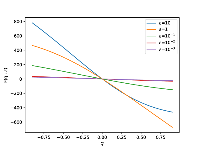
The learned is illustrated in Figure 5.1. Clearly, it is a strictly decreasing function of for each Knudsen number . This monotonicity guarantees the strictly concavity of the entropy function and thereby the conservation-dissipation principle.
5.3 Prediction
To show the performance of the CDF-based machine learning model (3.5), we solve it numerically and compare the numerical solutions with those computed from the kinetic equation (3.2). To compute the solutions, we discretize the learned balance laws (3.5) by using the Lax-Friedrichs scheme with a relatively fine mesh. The scheme is first-order, monotone and can produce entropy solutions in the presence of shocks.
Let be the solution computed by the scheme and be the solution generated by the BGK model (3.2) with the same initial data. We define their relative and errors as
and
where and are the values of and at the -th spatial grid point and the final time . We note that the prediction solution is computed by the Lax-Friedrich scheme with a refined mesh grid .
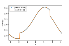
The relative errors for smooth and discontinuous solutions are given in Table 5.1 and Table 5.2, respectively. The mean and the standard derivation (std) are taken from 10 randomly different runs. From Table 5.1 and Table 5.2, we see that the magnitude of relative errors is less than 3% for smooth solutions and 6% for discontinuous solutions. Moreover, the errors become larger for larger Knudsen number , which is reasonable because it is more difficult to model non-equilibrium flows.
It is remarkable that although only the smooth training data are used to learn the balance laws (3.5), the learned model performs well also with the discontinuous initial data.
| relative error | relative error \bigstrut | |||
| Knudsen number | mean | std | mean | std \bigstrut |
| 2.46e-03 | 4.13e-04 | 2.62e-03 | 4.32e-04 \bigstrut[t] | |
| 1.72e-03 | 1.57e-04 | 1.89e-03 | 1.35e-04 | |
| 7.83e-03 | 2.62e-03 | 8.39e-03 | 2.71e-03 | |
| 2.17e-02 | 6.68e-03 | 2.33e-02 | 7.14e-03 | |
| 2.18e-02 | 5.37e-03 | 2.35e-02 | 5.73e-03 \bigstrut[b] | |
| relative error | relative error \bigstrut | |||
| Knudsen number | mean | std | mean | std \bigstrut |
| 1.03e-02 | 1.12e-03 | 1.49e-02 | 2.24e-03 \bigstrut[t] | |
| 6.30e-03 | 1.06e-03 | 8.60e-03 | 1.81e-03 | |
| 2.25e-02 | 2.65e-03 | 2.66e-02 | 3.02e-03 | |
| 4.54e-02 | 6.32e-03 | 5.16e-02 | 6.62e-03 | |
| 5.37e-02 | 1.06e-02 | 6.05e-02 | 1.20e-02 \bigstrut[b] | |
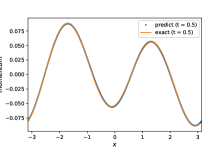
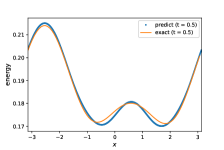
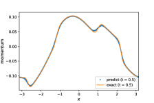
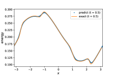
Furthermore, we plot the solution profiles of density, momentum, and energy obtained from the kinetic equation and the learned model at and . Figure 5.2 is for smooth initial data with in (5.1), which are not used in the training data, and with Knudsen number . Here and below, the ‘exact’ means that obtained from the kinetic equation while ‘predict’ is for the learned model. It is observed that the solution profiles of our model agree well with those of the BGK model. The performances with other Knudsen numbers are similar and are omitted here.
[5pt]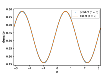 (i) density at
\stackunder[5pt]
 (ii) momentum at
\stackunder[5pt]
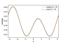 (iii) energy at
\stackunder[5pt]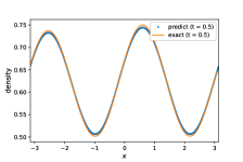 (i’) density at
\stackunder[5pt]
 (ii’)
momentum at
\stackunder[5pt]
 (iii’)
energy at
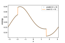
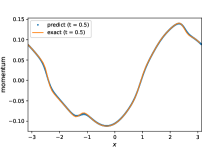
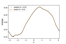
Below is the solution profiles with discontinuous initial data. Figures 5.3-5.7 are for different Knudsen numbers and . For small Knudsen numbers (), our learned model agrees quite well with the BGK model, see Figures 5.3-5.5. However, the deviation becomes large for and 10, see Figures 5.6 and 5.7.
[5pt]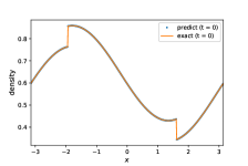 (i) density at
\stackunder[5pt]
 (ii) momentum at
\stackunder[5pt]
 (iii) energy at
\stackunder[5pt]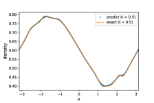 (i’) density at
\stackunder[5pt]
 (ii’)
momentum at
\stackunder[5pt]
 (iii’)
energy at
[5pt]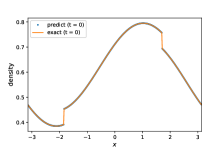 (i) density at
\stackunder[5pt]
 (ii) momentum at
\stackunder[5pt]
 (iii) energy at
\stackunder[5pt]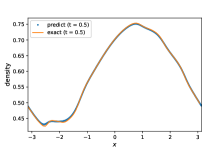 (i’) density at
\stackunder[5pt]
 (ii’)
momentum at
\stackunder[5pt]
 (iii’)
energy at
[5pt]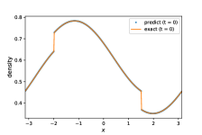 (i) density at
\stackunder[5pt]
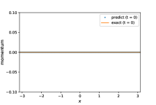 (ii) momentum at
\stackunder[5pt]
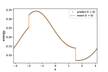 (iii) energy at
\stackunder[5pt]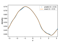 (i’) density at
\stackunder[5pt]
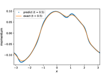 (ii’)
momentum at
\stackunder[5pt]
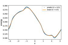 (iii’)
energy at
[5pt]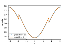 (i) density at
\stackunder[5pt]
 (ii) momentum at
\stackunder[5pt]
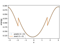 (iii) energy at
\stackunder[5pt]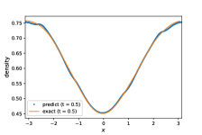 (i’) density at
\stackunder[5pt]
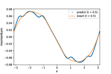 (ii’)
momentum at
\stackunder[5pt]
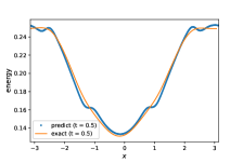 (iii’)
energy at
[5pt]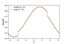 (i) density at
\stackunder[5pt]
 (ii) momentum at
\stackunder[5pt]
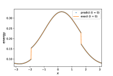 (iii) energy at
\stackunder[5pt]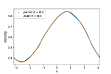 (i’) density at
\stackunder[5pt]
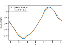 (ii’)
momentum at
\stackunder[5pt]
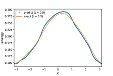 (iii’)
energy at
We further examine our model on Sod’s shock tube problem [35] with initial data
| (5.3) |
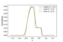
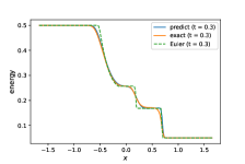
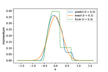
With these initial data, we numerically solve our model, the Euler equations and the kinetic equation up to . In the computations of our learned equations and the Euler equations, we use the Lax-Friedrich scheme with . The solution profiles of density, momentum, and energy obtained from the three models are shown in Figure 5.8 and Figure 5.9 with Knudsen number and .
From Figure 5.8 with , it is observed that the solution profiles of our model agree quite well with those of the BGK model. In contrast, the Euler equations generate sharp discontinuity, which deviates from the BGK model. On the other hand, Figure 5.9 is for larger Knudsen number . In this case, it is far away from equilibrium and difficult to build a good macroscopic model. We observe that the solutions of the Euler equations are quite different from those of the kinetic model, while our learned model also has a slight discrepancy but can well capture the tendency of the solution. The discrepancy may be due to the fact that only one non-equilibrium variable is introduced in our model. The poor behavior was also observed for the moment closure systems with few number of moments and improved with larger number of moments [6, 7]. Thus, we expect that the discrepancy could be reduced by adding more non-equilibrium variables under the CDF framework and this is left for future work.
[5pt]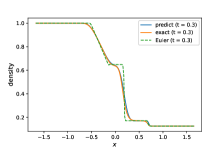 (i) density at
\stackunder[5pt]
 (ii)
momentum at
\stackunder[5pt]
 (iii)
energy at
[5pt]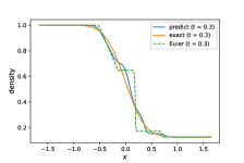 (i) density at
\stackunder[5pt]
 (ii)
momentum at
\stackunder[5pt]
 (iii)
energy at
6 Concluding remarks
In this work, we advocate combining machine learning with non-equilibrium thermodynamics. Precisely, we develop a method for learning interpretable, thermodynamically stable and Galilean invariant PDEs based on CDF. As governing equations for one-dimensional non-equilibrium flows, the learned PDEs are parameterized by fully-connected neural networks and satisfy the conservation-dissipation principle automatically. In particular, they are hyperbolic balance laws.
The training data are generated from the BGK model with smooth initial data. Numerical results indicate that our CDF-based machine learning model achieves good accuracy in a wide range of Knudsen numbers. It is remarkable that the learned dynamics can give satisfactory results with randomly sampled discontinuous initial data although it is trained only with smooth initial data. Particularly, for the classical Sod’s shock tube problem, our model behaves much better than the Euler equations.
This work could be improved in the following aspects: (1) Our model has only one non-equilibrium variable which may not be the best. Better numerical results are expected by introducing more non-equilibrium variables. (2) Only one-dimensional problems are considered here. It is more challenging to generalize our method to problems in multi-dimension.
Acknowledgment
JH would like to thank Qi Tang in Los Alamos National Laboratory for helpful discussions in training of the neural networks.
References
- [1] B. Amos, L. Xu, and J. Z. Kolter. Input convex neural networks. In International Conference on Machine Learning, pages 146–155, 2017.
- [2] U. M. Ascher, S. J. Ruuth, and R. J. Spiteri. Implicit-explicit Runge-Kutta methods for time-dependent partial differential equations. Applied Numerical Mathematics, 25(2-3):151–167, 1997.
- [3] A. G. Baydin, B. A. Pearlmutter, A. A. Radul, and J. M. Siskind. Automatic differentiation in machine learning: a survey. The Journal of Machine Learning Research, 18(1):5595–5637, 2017.
- [4] S. L. Brunton, J. L. Proctor, and J. N. Kutz. Discovering governing equations from data by sparse identification of nonlinear dynamical systems. Proceedings of the national academy of sciences, 113(15):3932–3937, 2016.
- [5] J. W. Burby, Q. Tang, and R. Maulik. Fast neural Poincaré maps for toroidal magnetic fields. arXiv preprint arXiv:2007.04496, 2020.
- [6] Z. Cai, Y. Fan, R. Li, and Z. Qiao. Dimension-reduced hyperbolic moment method for the Boltzmann equation with BGK-type collision. Communications in Computational Physics, 15(5):1368–1406, 2014.
- [7] Z. Cai and R. Li. Numerical regularized moment method of arbitrary order for Boltzmann-BGK equation. SIAM Journal on Scientific Computing, 32(5):2875–2907, 2010.
- [8] X. Chen, L. Yang, J. Duan, and G. E. Karniadakis. Solving inverse stochastic problems from discrete particle observations using the fokker-planck equation and physics-informed neural networks. arXiv preprint arXiv:2008.10653, 2020.
- [9] C. M. Dafermos. Hyperbolic Conservation Laws in Continuum Physics, volume 3. Springer, 2005.
- [10] S. R. De Groot and P. Mazur. Non-equilibrium Thermodynamics. Courier Corporation, 2013.
- [11] K. O. Friedrichs and P. D. Lax. Systems of conservation equations with a convex extension. Proceedings of the National Academy of Sciences, 68(8):1686–1688, 1971.
- [12] S. K. Godunov. An interesting class of quasilinear systems. In Dokl. Acad. Nauk SSSR, volume 139, pages 521–523, 1961.
- [13] S. Greydanus, M. Dzamba, and J. Yosinski. Hamiltonian neural networks. In Advances in Neural Information Processing Systems, pages 15379–15389, 2019.
- [14] J. Han, C. Ma, Z. Ma, and W. E. Uniformly accurate machine learning-based hydrodynamic models for kinetic equations. Proceedings of the National Academy of Sciences, 116(44):21983–21991, 2019.
- [15] J. Han, L. Zhang, R. Car, and W. E. Deep potential: A general representation of a many-body potential energy surface. arXiv preprint arXiv:1707.01478, 2017.
- [16] J. Han, L. Zhang, and W. E. Integrating machine learning with physics-based modeling. arXiv preprint arXiv:2006.02619, 2020.
- [17] Y. Hyon, D. Y. Kwak, and C. Liu. Energetic variational approach in complex fluids: maximum dissipation principle. Discrete & Continuous Dynamical Systems-A, 26(4):1291, 2010.
- [18] G.-S. Jiang and C.-W. Shu. Efficient implementation of weighted ENO schemes. Journal of Computational Physics, 126(1):202–228, 1996.
- [19] P. Jin, A. Zhu, G. E. Karniadakis, and Y. Tang. Symplectic networks: Intrinsic structure-preserving networks for identifying Hamiltonian systems. arXiv preprint arXiv:2001.03750, 2020.
- [20] D. Jou, J. Casas-Vázquez, and G. Lebon. Extended Irreversible Thermodynamics. In Extended Irreversible Thermodynamics, pages 41–74. Springer, 1996.
- [21] J. Z. Kolter and G. Manek. Learning stable deep dynamics models. In Advances in Neural Information Processing Systems, pages 11128–11136, 2019.
- [22] G. Lebon, D. Jou, and J. Casas-Vázquez. Understanding Non-equilibrium Thermodynamics, volume 295. Springer, 2008.
- [23] H. Lei, L. Wu, and W. E. Machine learning based non-Newtonian fluid model with molecular fidelity. arXiv preprint arXiv:2003.03672, 2020.
- [24] J. Ling, A. Kurzawski, and J. Templeton. Reynolds averaged turbulence modelling using deep neural networks with embedded invariance. Journal of Fluid Mechanics, 807:155–166, 2016.
- [25] Z. Long, Y. Lu, and B. Dong. PDE-Net 2.0: Learning PDEs from data with a numeric-symbolic hybrid deep network. Journal of Computational Physics, 399:108925, 2019.
- [26] Z. Long, Y. Lu, X. Ma, and B. Dong. PDE-Net: Learning PDEs from data. In International Conference on Machine Learning, pages 3208–3216, 2018.
- [27] I. Müller and T. Ruggeri. Rational Extended Thermodynamics. 1998.
- [28] W. Muschik. Contact temperature and internal variables: A glance back, 20 years later. Journal of Non-Equilibrium Thermodynamics, 39(3):113–121, 2014.
- [29] H. C. Öttinger. Beyond equilibrium thermodynamics. John Wiley & Sons, 2005.
- [30] M. Pavelka, V. Klika, and M. Grmela. Multiscale Thermo-dynamics: Introduction to GENERIC. Walter de Gruyter GmbH & Co KG, 2018.
- [31] M. Raissi and G. E. Karniadakis. Hidden physics models: Machine learning of nonlinear partial differential equations. Journal of Computational Physics, 357:125–141, 2018.
- [32] M. Raissi, P. Perdikaris, and G. E. Karniadakis. Physics-informed neural networks: A deep learning framework for solving forward and inverse problems involving nonlinear partial differential equations. Journal of Computational Physics, 378:686–707, 2019.
- [33] S. Ruder. An overview of gradient descent optimization algorithms. arXiv preprint arXiv:1609.04747, 2016.
- [34] S. Rudy, A. Alla, S. L. Brunton, and J. N. Kutz. Data-driven identification of parametric partial differential equations. SIAM Journal on Applied Dynamical Systems, 18(2):643–660, 2019.
- [35] G. A. Sod. A survey of several finite difference methods for systems of nonlinear hyperbolic conservation laws. Journal of Computational Physics, 27(1):1–31, 1978.
- [36] H. Struchtrup. Macroscopic transport equations for rarefied gas flows. In Macroscopic Transport Equations for Rarefied Gas Flows, pages 145–160. Springer, 2005.
- [37] P. Toth, D. J. Rezende, A. Jaegle, S. Racanière, A. Botev, and I. Higgins. Hamiltonian generative networks. arXiv preprint arXiv:1909.13789, 2019.
- [38] H. Wang, L. Zhang, J. Han, and W. E. Deepmd-kit: A deep learning package for many-body potential energy representation and molecular dynamics. Computer Physics Communications, 228:178–184, 2018.
- [39] M. Yin, X. Zheng, J. D. Humphrey, and G. E. Karniadakis. Non-invasive inference of thrombus material properties with physics-informed neural networks. arXiv preprint arXiv:2005.11380, 2020.
- [40] W.-A. Yong. An interesting class of partial differential equations. Journal of Mathematical Physics, 49(3):033503, 2008.
- [41] W.-A. Yong. Intrinsic properties of conservation-dissipation formalism of irreversible thermodynamics. Philosophical Transactions of the Royal Society A, 378(2170):20190177, 2020.
- [42] H. Yu, X. Tian, W. E, and Q. Li. OnsagerNet: Learning stable and interpretable dynamics using a generalized Onsager principle. arXiv preprint arXiv:2009.02327, 2020.
- [43] E. Zhang, M. Yin, and G. E. Karniadakis. Physics-informed neural networks for nonhomogeneous material identification in elasticity imaging. arXiv preprint arXiv:2009.04525, 2020.
- [44] L. Zhang, J. Han, H. Wang, R. Car, and W. E. Deep potential molecular dynamics: a scalable model with the accuracy of quantum mechanics. Physical Review Letters, 120(14):143001, 2018.
- [45] L. Zhang, J. Han, H. Wang, W. Saidi, R. Car, and W. E. End-to-end symmetry preserving inter-atomic potential energy model for finite and extended systems. In Advances in Neural Information Processing Systems, pages 4436–4446, 2018.
- [46] Y. D. Zhong, B. Dey, and A. Chakraborty. Symplectic ODE-net: Learning Hamiltonian dynamics with control. arXiv preprint arXiv:1909.12077, 2019.
- [47] Y. Zhu, L. Hong, Z. Yang, and W.-A. Yong. Conservation-dissipation formalism of irreversible thermodynamics. Journal of Non-Equilibrium Thermodynamics, 40(2):67–74, 2015.