The Probabilistic Description Logic
Abstract
Description logics (DLs) are well-known knowledge representation formalisms focused on the representation of terminological knowledge. Due to their first-order semantics, these languages (in their classical form) are not suitable for representing and handling uncertainty. A probabilistic extension of a light-weight DL was recently proposed for dealing with certain knowledge occurring in uncertain contexts. In this paper, we continue that line of research by introducing the Bayesian extension of the propositionally closed DL . We present a tableau-based procedure for deciding consistency, and adapt it to solve other probabilistic, contextual, and general inferences in this logic. We also show that all these problems remain ExpTime-complete, the same as reasoning in the underlying classical . Under consideration in Theory and Practice of Logic Programming (TPLP).
1 Introduction
Description logics (DLs) [Baader et al. (2007)] are a family of logic-based knowledge representation formalisms designed to describe the terminological knowledge of an application domain. Description Logics have been successfully applied to model several domains, with some particularly successful applications coming from the biomedical sciences. This is due to their clear syntax, formal semantics, the existence of efficient reasoners, and their expressivity. However, in their classical form, these logics are not capable of dealing with uncertainty, which is an unavoidable staple in real-world knowledge. To overcome this limitation, several probabilistic extensions of DLs have been suggested in the literature. The landscape of probabilistic extensions of DLs is too large to be covered in detail in this work. These logics differentiate themselves according to their underlying logical formalism, their interpretation of probabilities, and the kind of uncertainty that they are able to express. For a relevant survey, where all these differences are showcased, we refer the interested reader to [Lukasiewicz and Straccia (2008)]. More recent work where probabilistic DLs are discussed can be found in [Ceylan and Lukasiewicz (2018), Gutiérrez-Basulto et al. (2017)].
A related probabilistic DL, called [Ceylan and Peñaloza (2017)], is the Bayesian extension of the light-weight [Baader et al. (2005)]. This logic focuses on modelling certain knowledge that holds only in some contexts, together with uncertainty about the current context. is based on a subjective interpretation of probabilities or, in Halpern’s terminology, it corresponds to a Type II probabilistic logic [Halpern (1990)]. One advantage of the formalism underlying is that it separates the contextual knowledge, which is de facto a classical ontology, from the likelihood of observing this context, which can be influenced by external factors. We present a simple example of the importance of contextual knowledge. Consider the knowledge of construction techniques and materials that vary through time. In the context of a modern house asbestos and lead pipes are not observable, while in some classes of houses, built during the 1970s, we observe both. However, in all contexts we know that asbestos and lead in drinking water have grave health effects. When confronted with a random house, one might not know to which of these contexts it belongs, and by extension whether it is safe to live in, or drink the water that flows through its pipes. Still, construction data may be used to derive the probabilities of these contexts.
To allow for complex probabilistic relationships between the contexts without needing to result to incompatible independence assumptions, their joint probability distribution is encoded via a Bayesian network (BN) [Pearl (1985)]. This logic is closely related to the probabilistic extension of DL-Lite [Artale et al. (2009)] proposed previously in [d’Amato et al. (2008)], but uses a less restrictive semantics which resembles more the open-world assumption from DLs (for a discussion on the differences between the semantics of these logics, see [Ceylan and Peñaloza (2017)]). Another similar proposal is Probabilistic Datalog± [Gottlob et al. (2013)], with the difference that uncertainty is represented via a Markov Logic Network, instead of a BN. Since the introduction of , the main notions behind it have been generalised to arbitrary ontology languages [Ceylan (2018)]. However, it has also been shown that efficient and complexity-optimal reasoning methods can only be achieved by studying the properties of each underlying ontology language [Ceylan and Peñaloza (2017)]. Finally, another family of probabilistic DLs using Type II semantics was proposed in [Gutiérrez-Basulto et al. (2017)], which we refer to as Prob-DLs. The biggest difference between Bayesian DLs and Prob-DLs is that the latter models uncertain concepts, while the former models uncertain knowledge. For example, Prob-DLs can refer to the class of all individuals having a high probability of a disease infection, but cannot express that an entailment holds with a given probability.
In this paper, we continue with that line of research and study the Bayesian extension of the propositionally closed DL . As our main result, we present an algorithm, based on a glass-box modification of the classical tableaux method for reasoning in . Our algorithm is able to derive those contexts which are needed to determine the (in)consistency of a knowledge base. Using this algorithm, we then describe an effective method for deciding consistency of a knowledge base. We also provide a tight ExpTime complexity bound for this problem.
This is followed by a study of several crisp and probabilistic variants of the standard DL decision problems; namely, concept satisfiability, subsumption, and instance checking. Interestingly, our work shows that all our problems can be reduced to some basic computations over a context describing inconsistency, and hence are ExpTime-complete as well. These complexity bounds are not completely surprising, given the high complexity of the classical . However, our tableaux-based algorithm has the potential to behave better in practical scenarios. This work details and deepens results that have previously been presented in [Botha (2018), Botha et al. (2018), Botha et al. (2019)]
2 Preliminaries
We start by providing a brief introduction to Bayesian networks and the description logic (DL) , which form the basis for the probabilistic DL . For a more detailed presentation of these topics, we refer the interested reader to [Darwiche (2009), Baader et al. (2017)]
2.1 Bayesian Networks
Bayesian networks (BNs) are graphical models, which are used for representing the joint probability distribution (JPD) of several discrete random variables in a compact manner [Pearl (1985)]. Before introducing these models formally, we need a few definitions.
Given a random variable , let denote the set of values that can take. For the scope of this paper, we consider only random variables such that is finite. For , denotes the valuation of taking the value . This notation is extended to sets of variables in the obvious way. Given a set of random variables , a world is a set of valuations containing exactly one valuation for every random variable . In other words, a world specifies an exact instantiation of all the variables in .
A -literal is an ordered pair of the form , where and . -literals are similar to valuations, but the syntactic difference is introduced to emphasise their difference in use, as will become clear later. -literals are a generalisation of Boolean literals, which are typically denoted as or for the Boolean random variable . For simplicity, and following this connection, in this paper we will often use the notation for and for . A -context is any set of -literals. A -context is consistent if it contains at most one literal for each random variable. We will often also call -contexts primitive contexts.
A Bayesian network is defined as a pair where is a directed acyclic graph (DAG) and is a set of conditional probability distributions for every variable given its parents on the DAG ; more precisely, this set has the form
The BN specifies a full JPD for the variables in by considering independence assumptions depicted in the graph ; namely, every variable is (conditionally) independent of all its non-descendants given its parents. Under this assumption, it is easy to see that the JPD of can be computed through the chain rule
that is, the probability of a world is obtained by multiplying the conditional probabilities of the valuations found in the tables. We let denote the JPD defined by the BN .
Example 1
Figure 1 depicts a BN with four random variables denoting the likelihood of different characteristics of a construction: stands for a post-1986 building, for a renovated building, for the presence of lead pipes, and for the safety of drinking water.
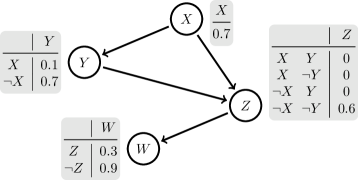
The tables attached to each node are the conditional probability distribution of that node given its parents. Hence, the BN expresses that a post-1986 building has only probability of being renovated.
The DAG expresses the conditional independence of and given . That is, once that we observe the value of (if we know whether a house has lead pipes or not) then the probability of is not affected by the knowledge of the renovation status of a house.
Through the chain rule, we can derive e.g.,
| and | ||||
That is, it is very unlikely to find an old, non-renovated house, with lead pipes, and unsafe water; and renovated post-1986 houses with safe water cannot have lead pipes. Note that to express the full JPD of these four variables directly, we would need a table with 16 rows.
2.2 The Description Logic
is the smallest propositionally closed DL [Baader et al. (2007), Schmidt-Schauß and Smolka (1991)]. As with all DLs, its fundamental notions are those of concepts which correspond to unary predicates of first-order logic, and roles corresponding to binary predicates. Formally, given the mutually disjoint sets , and of individual, concept, and role names, respectively, the class of concepts is built through the grammar rule
where and .
The knowledge from an application domain is represented through a set of axioms, which restrict the possible interpretations of concepts and roles. In , axioms are either general concept inclusions (GCIs) of the form , concept assertions , or role assertions where , and are concepts. An ontology is a finite set of axioms. As customary in DLs, we sometimes partition an ontology into the TBox composed exclusively of GCIs, and the ABox containing all concept and role assertions, when it is relevant which kind of axiom is being used.
The semantics of is defined by interpretations akin to the first-order semantics. An interpretation is a pair of the form where is a non-empty set called the domain and is the interpretation function that maps every to an element , every to a set and every to a binary relation . This interpretation function is inductively extended to arbitrary concepts by defining for any two concepts :
-
•
,
-
•
,
-
•
,
-
•
, and
-
•
.
The interpretation satisfies the GCI iff ; the concept assertion iff ; and the role assertion iff . We denote as if satisfies the axiom . is a model of the ontology (denoted by ) iff it satisfies all axioms in .
An important abbreviation in is the bottom concept , where is any concept name. Clearly, this concept stands for a contradiction and, for any interpretation , . Similarly, the top concept stands for a tautology and holds for every interpretation .
The basic reasoning task in consists in deciding whether a given ontology is consistent; that is, whether there exists a model of . This problem is known to be ExpTime-complete [Schild (1991), Donini and Massacci (2000)]. Other reasoning problems, such as subsumption and instance checking, can be polynomially reduced to this one and hence preserve the same complexity.
Example 2
In it is possible to express the notion that water pipes do not contain lead through the GCI . In addition, we can express that the object is a water pipe (); that contains by the assertion ; and that is in fact lead (). Note that the ontology containing all four axioms is inconsistent.
3
We now introduce the probabilistic DL , which combines BNs, to compactly express joint probability distributions, and to express background knowledge. In addition, can express logical (as opposed to probabilistic) dependencies between axioms. More precisely, axioms are required to hold only in some (possibly uncertain) contexts, which are expressed through annotations. The uncertainty of these contexts is expressed by the BN. These ideas are formalised next.
Definition 3 (KB)
Let be a finite set of discrete random variables. A -restricted axiom (-axiom) is an expression of the form , where is an axiom and is a -context. A -ontology is a finite set of -axioms. A knowledge base (KB) over is a pair where is a BN over , and is a -ontology.
Note that the contexts labelling the axioms, and the variables of the BN from a KB both come from the same set of discrete random variables .
To define the semantics of , we extend the notion of an interpretation from to also take contexts into account. The probabilities expressed by the BN are associated to the axioms following the multiple-world approach.
Definition 4 (-interpretation)
Let be a finite set of discrete random variables. A -interpretation is a tuple of the form where is an interpretation and is a valuation function which maps every to some .
Given a valuation function , a Bayesian world , and a context we use the notation to express that assigns to each random variable the same value as it has in ; to state that for all ; and when there is such that .
Definition 5 (Model)
The -interpretation is a model of the -axiom (denoted as ) iff (i) , or (ii) satisfies . is a model of the ontology iff it is a model of all axioms in . In this case, we denote it by .
It is important to notice at this point that is a generalisation of the classical DL . Recall that a -context is a set of -literals; that is, of pairs . In particular, the empty set of literals is also a -context. By definition, every valuation function is such that . This means that the axiom is equivalent to the -axiom . As a whole every ontology can be seen as a -ontology by simply associating the empty context to all its axioms. The original ontology and the -ontology constructed this way have the same class of models, except that the latter allows for any arbitrary valuation function in its third component. For brevity, and the reasons just described, for the rest of this paper we will abbreviate axioms of the form simply as . When it is clear from the context, we will also omit the prefix and refer only to e.g. contexts, GCIs, or ontologies.
A -interpretation—more precisely, its valuation function—refers to only one possible world of the random variables in . KBs, on the other hand, have information about the uncertainty of being in one world or another. In the multiple-world semantics, probabilistic interpretations combine multiple -interpretations and the probability distribution described by the BN to give information about the uncertainty of the axioms, and their consequences.
Definition 6 (Probabilistic model)
A probabilistic interpretation is a pair of the form , where is a finite set of -interpretations and is a probability distribution over such that for all . The probabilistic interpretation is a model of the axiom (denoted by ) iff every is a model of . is a model of the ontology iff every is a model of .
We say that the probability distribution is consistent with the BN if for every possible world of the variables in it holds that
Recall that denotes the joint probability distribution defined by the BN . The probabilistic interpretation is a model of the KB iff it is a (probabilistic) model of , and is consistent with .
In other words, a probabilistic interpretation describes a class of possible worlds, in which the knowledge of is interpreted, and each world is associated with a probability. For this interpretation to be a model of the KB, it has to satisfy the constraints it requires; that is, the ontological knowledge must be satisfied in each world, and the probabilities should be coherent with the distribution from the BN.
Example 7
Consider the KB where is the BN depicted in Figure 1, and is the ontology
The first axiom provides a partial definition, stating that every pipe which contains lead is a lead pipe. Note that it is labelled with the empty context, which means that it always holds. The two axioms in the second row express that pipes in post-1986 (that is, within the context ) and in renovated buildings (in context ) do not contain lead.
The axioms in the third row refer exclusively to the context of lead pipes (). In this case, our knowledge is that pipes do contain lead, and that water with low alkalinity is not drinkable, as it absorbs the lead from the pipes it travels on. Notice that the axioms in the second row contradict appearing in the third row. This is not a problem because they are required to hold in different contexts. Indeed, we can observe from Figure 1 that any context which makes , and either or true must have probability 0. This means that no probabilistic model can contain a world that satisfies these conditions.
Finally, the last two axioms state that water at a building is drinkable iff we are in the context of drinkable water (). Note that it is important to provide both axioms in order to guarantee an equivalence. Suppose that we had not included the last axiom (i.e., ). Then, by our semantics, we could still produce a -interpretation whose valuation satisfies but such that . This can only be avoided by the introduction of the last axiom.
It is a simple exercise to verify that this ontology has a model. The smallest probabilistic model of the KB contains 10 -interpretations; one for each world with positive probability.
Recall that -contexts are also called primitive contexts. This is to emphasise the difference with what we will, from now on, call complex contexts. Formally, a complex context is a finite non-empty set of primitive contexts. Note that primitive contexts can be seen as complex ones; e.g., the primitive context corresponds to the complex context , and we will use them interchangeably when there is no risk of ambiguity.
Given a valuation function and a complex context we say that satisfies (written as ) iff satisfies at least one ; in particular, iff . Thus, for the rest of the paper we assume that all contexts are in complex form unless explicitly stated otherwise. We emphasise here that for a valuation function to satisfy a complex context, it suffices that it satisfies one of the simple contexts in it. Intuitively, a simple context is a conjunction of valuations, while a complex context is a disjunction of simple contexts. However, one should not forget that the variables appearing in these contexts can potentially take more than two different values.
Definition 8
Given complex contexts and we define the operations
| and | ||||
These operations generalise propositional disjunction () and propositional conjunction (), where disjunction has the property that either one of the two contexts holds and conjunction requires that both hold.
Given two complex contexts and , we say that entails (denoted by ) iff for all such that it follows that . Alternatively holds iff for all Bayesian worlds such that it follows that . It is easy to see that for all worlds and complex contexts it holds that (i) iff or , and (ii) iff and . Two important special complex contexts are top () and bottom (), which are satisfied by all or no world, respectively. If there are consistent primitive contexts and is an inconsistent context, these are defined as and .
This concludes the definition of the relevant components of the logic . In the next section, we study the problem of consistency of a KB, and its relation to other reasoning problems.
4 Consistency
As for , the most basic decision problem one can consider in is consistency. Formally this problem consists of deciding whether a given KB has a probabilistic model or not. To deal with this problem it is convenient to consider the classical ontologies that should hold at each specific world, which we call the restriction.
Definition 9 (restriction)
Given the KB and the world , the restriction of to is the ontology defined by
Recall that a probabilistic model of is a class of classical interpretations associated to worlds , where each is a model of the -ontology . For such an interpretation to be a model of , it must hold that, for each axiom such that , (see Definition 5). This condition is equivalent to stating that is a classical model of .
Example 10
Consider the KB from Example 7, and the two worlds and . We then have
| and | ||||
Note that both ontologies are consistent, but can only be satisfied by interpretations such that .
In addition to satisfying the restrictions, the probability distribution of a model must be consistent with the BN . This means that the probabilities of the interpretations associated with the world must add to . Using this insight, we obtain the following result.
Theorem 11
The KB is consistent iff for every world with it holds that is consistent.
Proof 4.12.
Suppose first that for every world such that the ontology is consistent. We build a probabilistic model of as follows. Given a world with , let be an arbitrary (classical) model of . We construct the -interpretation ; that is, the same interpretation , but associated to the world . We claim that . Indeed, take an arbitrary . If , then trivially. Otherwise, and hence (since ) . Let now be the set of all worlds such that . We define the set of -interpretations , and the probability distribution that sets for every . The probabilistic interpretation is a model of .
Conversely, suppose that is consistent, and let be a model of . Given a world such that , we know that . In particular this means that there must exist some such that . means that and hence . Thus, is consistent.
Based on this result, we can derive a process for deciding consistency that provides a tight complexity bound for this problem.
Corollary 4.13.
KB consistency is ExpTime-complete.
Proof 4.14.
Recall that consistency checking in is ExpTime-complete, and that is a generalisation of . This yields ExpTime-hardness for consistency. To obtain the upper bound, note that there are exponentially many worlds . For each of them, we can check (classical) consistency of (in exponential time) and that , which is linear in the size of by the chain rule.
The algorithm described in the proof of this corollary is optimal in terms of worst-case complexity, but it also runs in exponential time in the best case. Indeed, it enumerates all the (exponentially many) Bayesian worlds, before being able to make any decision. In practice, it is infeasible to use an algorithm that requires exponential time on every instance. For that reason, we present a new algorithm based on the tableau method originally developed for . To describe this algorithm, we need to introduce some additional notation.
We denote the context that describes all worlds such that is inconsistent as . That is, the context is such that iff is inconsistent. Moreover, is a context such that iff . Theorem 11 states that is inconsistent whenever there is a world that models both and . This is formalized in the following result.
Theorem 4.15.
Given the KB , let and be the contexts described above. Then is inconsistent iff is satisfiable.
Proof 4.16.
is inconsistent iff there is a world such that and is inconsistent (Theorem 11) iff and iff iff is satisfiable.
Example 4.17.
Consider once again the KB from Example 7, and notice that is consistent for all worlds . Hence . In particular, this means that is unsatisfiable, and hence is consistent.
Let now , where . We can see that for any world which entails any of the contexts or , is inconsistent. Hence we have that . Looking at the probability tables from , we also see that ; that is, any world that satisfies or must have probability 0. Thus, and is consistent as well.
To decide consistency, it then suffices to find a method which is capable of deriving the contexts and . For the former, we present a variant of the glass-box approach for so-called axiom pinpointing [Lee et al. (2006), Meyer et al. (2006), Baader and Peñaloza (2010)], which is originally based on the ideas from [Baader and Hollunder (1995)]. This approach modifies the standard tableaux algorithm for —which tries to construct a model by decomposing complex constraints into simpler ones—to additionally keep track of the contexts in which the derived elements from the tableau hold. In a nutshell, tableau algorithms apply different decomposition rules to make implicit constraints explicit. For axiom pinpointing, whenever a rule application requires the use of an axiom from the ontology, this fact is registered as part of a propositional formula. In our case, we need a context, rather than a propositional formula, to take care of the multiple values that the random variables take. Although the underlying idea remains essentially unchanged, the handling of these multiple values requires additional technicalities. Before we look at this algorithm in detail, it is important to keep in mind that the goal is to detect all the worlds whose restriction is an inconsistent ontology; hence, we are interested in detecting and highlighting contradictions.
For this algorithm, it will be important to distinguish the terminological portion of the ontology (the TBox) from the assertional knowledge (the ABox). From a very high-level view, the algorithm starts by creating a partial model that satisfies all the constraints from the ABox, and then uses rules to decompose complex concepts until an actual valuation (based exclusively on concept names and role names) is reached. Throughout the process, rules are also used to guarantee that all the constraints from the TBox are satisfied by the individuals in this model.
The algorithm starts with the ABox from . If contains no assertions, we assume implicitly that the ABox is for an arbitrary individual name . Recall that all the axioms in are labeled with a context, and we preserve the context at this initialisation step. From this point, the algorithm deals with a set of ABoxes , which are created and modified following the rules from Figure 2.
| -rule | if | , and either or is -insertable |
| then | ||
| -rule | if | , and both and are -insertable |
| then | , | |
| -rule | if | , there is no such that neither nor is -insertable, and is not blocked |
| then | , where is a new individual name | |
| -rule | if | , and is -insertable |
| then | ||
| -rule | if | , appears in , and is -insertable |
| then |
Throughout the execution of the algorithm, each assertion in the ABoxes is labelled with a context which, as usual, is a propositional formula over the context variables; the algorithm modifies these labels accordingly to store all the relevant information. As a pre-requisite for the execution of the algorithm, we assume that all concepts appearing in the ontology are in negation normal form (NNF); that is, only concept names can appear in the scope of a negation operator. This assumption is made w.l.o.g. because every concept can be transformed into NNF in linear time by applying the De Morgan laws, the duality of the quantifiers, and eliminating double negations. Each rule application chooses an ABox and replaces it by one or two new ABoxes that expand with new assertions. We explain the details of these rule applications next.
An assertion is -insertable iff for all such that , . In the expansion rules, the symbol is used as shorthand for the operation
The main idea of this operator is to update the contexts in which an assertion is required to hold. Either the assertion is not already present in the ABox, and hence it is included with the context obtained by conjoining all the contexts triggering the rule application or, if the assertion is already present, there are multiple ways to derive the same assertion, whose contextual causes are all disjoint. Rather than keeping two different assertions in the ABox, we simply update its label.
Within an ABox , we say that the individual is an ancestor of if there is a chain of role assertions connecting to ; more formally, if there exist role names and individuals with such that , , and . The node blocks iff is an ancestor of and for every , there is a such that and ; is blocked if there is a node that blocks it.
The algorithm applies the expansion rules from Figure 2 until is saturated; i.e., until no rule is applicable to any . We say that the ABox contains a clash if for some individual and concept name . Informally, a clash means that the ABox has an obvious contradiction, as it requires to interpret the element to belong to the concept and its negation. We define the context
which intuitively describes the contexts of all the clashes that appear in . When is saturated, we return the context expressing the need of having clashes in every ABox for inconsistency to follow. This is because each ABox in is a potential model, where the multiplicity arises from the non-deterministic choice when decomposing disjunctions . If all potential choices are obviously contradictory, then no model can exist. It is important for the correctness of the algorithm to notice that the definition of a clash does not impose any constraints on the contexts and labelling the assertions and , respectively. Indeed, and could hold in contradictory contexts. In that case, the conjunction appearing in would not be affected; i.e., this clash will not provide any new information about inconsistency. For example, if , then the context is . This context cannot be satisfied by any world, meaning that is not inconsistent.
Informally, the context corresponds to the clash formula (also called pinpointing formula) for explaining inconsistency of an ontology [Lee et al. (2006), Baader and Peñaloza (2010)]. The main differences are that the variables appearing in a context are not necessarily Boolean, but multi-valued, and that the axioms in are not labelled with unique variables, but rather with contexts. The correctness of the approach follows from the fact that each assertion is labelled with a formula representing the contexts in which is necessarily true. Thus, every inconsistent context will be represented in . Conversely, saturation of the expansion rules guarantees that no other derivations of inconsistency as possible; otherwise, some rule would still be applicable.
Notice that the expansion rules in Figure 2 generalise the expansion rules for , but may require new rule applications to guarantee that all possible derivations of a clash are detected. Indeed, while the classical algorithm never applies a rule where the derived assertion already exists in the ABox, our modified algorithm may apply the rule if the label associated to the assertion does not already imply that which will be included. As observed in [Baader and Peñaloza (2007), Baader and Peñaloza (2010)], one has to be careful with claims of termination of the modified method, since the additional rule applications may in fact lead to an infinite execution. Specifically, the modified algorithm obtained from a terminating tableau is not guaranteed to terminate. However, [Baader and Peñaloza (2010), Peñaloza (2009)] devised some general conditions, which are sufficient to guarantee termination of a method modified in this way. Importantly, those conditions are met whenever the original algorithm deals only with unary and binary assertions, as is the case of the algorithm presented here. Hence, our approach is also guaranteed to terminate. This yields the following result.
Theorem 4.18.
The modified tableau algorithm terminates, and the context is such that for every world , iff is inconsistent.
The proof of this theorem is analogous to the proofs of correctness and termination of pinpointing extensions for tableau algorithms from [Baader and Peñaloza (2010)] only taking the differences between propositional formulas and contexts into account.
We now turn our attention to the computation of the formula . Recall that in a BN, the joint probability distribution is the product of the conditional probabilities of each variable given its parents. Hence a world can only have probability 0 if it evaluates some variable in and its parents to values and , respectively, such that . Thus, to compute it suffices to find out the cells in the conditional probability tables in with value .
Theorem 4.19.
Let be a BN, and define
Then for every world , iff .
Proof 4.20.
If then there is a variable such that and . By the chain rule it follows that . Conversely, if it must be the case that at least one factor in the product is 0; but then that factor satisfies a disjunct in .
Notice that, in general, the context can be computed faster than simply enumerating all possible worlds. In particular, if the conditional probability tables in contain no 0-valued cell, then ; i.e., it is satisfied by no world.
To summarise, in this section we have shown that deciding inconsistency of a KB can be reduced to checking satisfiability of the context , where is the context representing all the worlds where is inconsistent, and is the context representing all worlds with . We then provided a tableaux-like method for computing , and an enumeration approach for finding . We note that, just like in classical , the tableau algorithm is not optimal in terms of computational complexity. In fact, although consistency of ontologies is in ExpTime [Donini and Massacci (2000)], the tableau algorithm we use as the basis of our approach runs in double exponential time; the main reason for this is the -rule which may duplicate the number of ABoxes under consideration. We conjecture that it can be implemented in a goal-directed manner which behaves well in practice, but leave this for future work.
Although consistency is a very important problem to be studied, we are interested also in other reasoning tasks, which can arise through the use of probabilistic ontologies. In particular, we should also take into account the contexts and the probabilities provided by the BN beyond the question of whether they are positive or not. In the next section we study variants of satisfiability and subsumption problems, before turning our attention to instance checking.
5 Satisfiability and Subsumption
In this section, we focus on two problems—satisfiability and subsumption—which depend only on the TBox part of an ontology, and hence assume for the sake of simplicity that the ABox is empty. Thus, we will often write a KB as a pair where is a TBox and is a BN. We are in general interested in understanding the properties and relationships of concepts.
Definition 5.21.
Given two concepts and a KB , we say that is satisfiable w.r.t. iff there exists a probabilistic model of s.t. for all . We say that is subsumed by w.r.t. iff for all models of and all .
It is possible to adapt the well known reductions from the classical case to show that these two problems are ExpTime-complete.
Theorem 5.22.
Satisfiability and subsumption w.r.t. KBs are ExpTime-complete.
Proof 5.23.
Let and be concepts. It is easy to see that is subsumed by w.r.t. iff the KB is inconsistent, where is an arbitrary individual name. Similarly, is satisfiable iff is consistent.
In the following, we study variants of these problems which take contexts and probabilities into account. For a more concise presentation, we will present only the cases for subsumption. Analogous results hold for satisfiability based on the fact that for every interpretation , it holds that iff ; hence, an approach that is similar to the one used to solve subsumption can be used to solve satisfiability. First we consider additional information about contexts; afterwards we compute the probability of an entailment, and finally the combination of both kinds of information.
Definition 5.24 (contextual subsumption).
Let be a KB, concepts, and a context. is subsumed by in context w.r.t. , denoted as , if every probabilistic model of is also a model of .
This definition introduces the natural extension of subsumption that considers also the contexts. Note that in our setting, contexts provide a means to express and reason with probabilities.
Definition 5.25 (subsumption probability).
Let be a probabilistic model of the KB , a context, and two concepts. The probability of w.r.t. is
The probability of w.r.t. is
We say that is positively subsumed by in iff ; it is -subsumed iff ; it is exactly -subsumed iff ; and it is almost certainly subsumed iff .
The definition above allows us to consider the problem of probabilistic reasoning. That is, the probability of a subsumption in a specific model is the sum of the probabilities of the worlds in which is subsumed by in context ; notice that this trivially includes all worlds where does not hold, by construction (see Definition 5). In the case where is inconsistent we define the probability of all subsumptions as to ensure our definition is consistent with general probability theory (recall that in general).
When we speak about the probability of a subsumption w.r.t. a KB, we consider the infimum over the probabilities provided by all possible models of . The reason for this is that we want to find the tightest constraint, taking into account the open world semantics. The infimum is, to a degree, the natural interpretation of the information that holds in all possible models. When reasoning about probabilities it is not always important to compute a precise value, but rather find some relevant bounds. Thus, -subsumption considers a lower bound, while positive subsumption only cares about the probability being zero or not (dually, almost-certainty refers to the probability being one or not). All these decision problems have different applications and properties.
Contextual subsumption is related to subsumption probability in the obvious way. Namely, a KB entails a contextual subsumption iff the probability of the subsumption in is 1.
Theorem 5.26.
Given a KB , concepts and , and a context , it holds that:
Proof 5.27.
iff for every probabilistic interpretation , if , then iff for every probabilistic model of and every , iff for every model of iff .
This is convenient as it provides a method of reusing our results from Section 4, which finds a context describing inconsistency, to compute subsumption probabilities.
Theorem 5.28.
Let be a consistent KB, two concepts, and a context. For the KB it holds that
Proof 5.29.
Let , so . For an arbitrary but fixed model of , we have that
Hence . For the lower bound, it suffices to build a minimal model of , where for each world we have an interpretation such that iff as in the proof of Theorem 11.
Example 5.30.
Returning to our running example with the KB from Example 7, suppose that we are interested in finding the probability of water being drinkable. That is, we want to compute . Since , Theorem 5.28 states that it suffices to find the probabilities of all worlds such that the restriction of to is inconsistent. We note that the only such worlds are those which satisfy . Hence,
Those worlds, and their probabilities, are shown in Table 1.
| world | ||||
|---|---|---|---|---|
| 0 | ||||
| 0.063 | ||||
| 0 | ||||
| 0.567 | ||||
| 0 | ||||
| 0.189 | ||||
| 0.0162 | ||||
| 0.0108 | ||||
Adding all these values we get that the probability is . In other words, according to our model, the probability of a building having drinkable water (in the absence of any other information) is very high.
Notice that the formula requires at most exponential space on the size of to be encoded. For each of the exponentially many worlds, computing requires polynomial time due to the chain rule. Hence, overall, the computation of the subsumption probabilities requires exponential time. Importantly, this bound does not depend on how was computed; it could have e.g. been computed through the process described in Corollary 4.13. This provides an exponential upper bound for computing the probability of a subsumption.
Corollary 5.31.
The probability of a subsumption w.r.t. a KB can be computed in exponential time on the size of the KB.
Obviously, an exponential-time upper bound for computing the exact probability of a subsumption relation immediately yields an ExpTime upper bound for deciding the other problems introduced in Definition 5.25 as well. All these problems are also generalisations of the subsumption problem in . More precisely, given an TBox , we can create the KB where contains all the axioms in labelled with the context and contains only one Boolean node that holds with probability 1. Given two concepts iff is almost certainly subsumed by in context . Since subsumption in is already ExpTime-hard, we get that all these problems are ExpTime-complete.
In practice, however, it may be too expensive to compute the exact probability when we are only interested in determining lower bounds, or the possibility of observing an entailment; for instance, when considering positive subsumption. Recall once again that, according to our semantics, a contextual GCI will hold in any world such that . Thus, if the probability of this world is positive (), we can immediately guarantee that . Thus, positive subsumption can be decided without any ontological reasoning for any context that is not almost certain. In all other cases, the problem can still be reduced to inconsistency.
Theorem 5.32.
Let be a consistent KB. The concept is positively subsumed by in context w.r.t. iff is inconsistent or .
Proof 5.33.
Assuming that is consistent, if , the result is an immediate consequence of Theorem 5.28. Otherwise, , and since is consistent, inconsistency of can only arise from the two new assertions, which means that and in particular .
This theorem requires the context to be specified to decide positive subsumption. If is not known before hand, it is also possible to leverage the inconsistency decision process, which is the most expensive part of this method; recall that otherwise we only need , which can be easily computed from . Let . That is, extends with assertions negating the subsumption relation, which should hold in all contexts. From Theorem 4.18 we conclude that encodes all the contexts in which must hold. Notice that the computation of does not depend on the context but can be used to decide positive subsumption for any context.
Corollary 5.34.
The concept is positively subsumed by in context w.r.t. iff entails or .
Considering the probabilities of contextual subsumption relations may lead to unexpected or unintuitive results arising from the contextual semantics. Indeed, it always holds (see Theorem 5.32) that . In other words, the probability of a subsumption in a very unlikely context will always be very high, regardless of the KB and concepts used. In essence, this is caused because the semantics of contextual subsumption impose a variation of a material implication—if holds, then the subsumption holds—which is vacuously true if the premise (if holds) is false. In some cases, it may be more meaningful to consider a conditional probability under the assumption that the context holds, as defined next.
Definition 5.35 (conditional subsumption).
Let be a probabilistic model of the KB , two contexts with , and two concepts. The conditional probability of given w.r.t. is
The conditional probability of given w.r.t. is
This definition follows the same principles of conditioning in probability theory, but extended to the open world interpretation provided by our model-based semantics. Notice that, in addition to the scaling factor in the denominator, the nominator is also differentiated from Definition 5.25 by considering only the worlds that satisfy the context already.
Notice that the conditional probabilities in Definition 5.35 are pretty similar to those in Definition 5.25, except that the sum restricts to only the worlds that satisfy the context . Thus, the numerator can be obtained from the contextual probability in the context excluding the worlds that violate . More formally, we have that
Thus we get the following result.
Theorem 5.36.
.
In particular, this means that also conditional probabilities can be computed through contextual probabilities, with a small overhead of computing the probability (on the BN ) of the conditioning context .
As in the contextual case, if one is only interested in knowing that the subsumption is possible (that is, that it has a positive probability), then one can exploit the complex context describing the inconsistent contexts which, as mentioned before, can be precompiled to obtain the contexts in which a subsumption relation must be satisfied. However, in this case, entailment between contexts is not sufficient; one must still compute the probability of the contextual subsumption.
Corollary 5.37.
Let be a consistent KB, concepts, and contexts s.t. . iff .
In other words, iff is -subsumed by in with .
Example 5.38.
Continuing Example 5.30, suppose that we know that the context holds; that is, the house was built before 1986. Following Theorem 5.36 we can compute
The denominator can be read directly from the probability distribution in Figure 1; that is, . From Theorem 5.28, the numerator becomes the sum of the probabilities of all worlds that become inconsistent with the addition of the assertions . These are the same appearing in the last four rows of Table 1. Hence,
As expected, knowing that the house is pre-1986 increases the probability of having lead tubing, which means a decrease in the probability of drinkable water.
Analogously to Definitions 5.24, 5.25, and 5.35, it is possible to define the notions of consistency of a concept to hold in only some contexts, and based on it, the (potentially conditional) probability of such a contextual consistency problem. As mentioned already, it is well known that for every interpretation it holds that iff . Hence, all these problems can be solved through a direct reduction to their related subsumption problem.
We now turn our attention to the problem of instance checking. In this problem, the ABox also plays a role. Hence, we consider once again ontologies that can have in addition to GCIs, concept and role assertions.
6 Instance Checking
We consider a probabilistic extension to the classical instance checking problem. In we call this problem probabilistic instance checking and we define both a decision problem and probability calculation for it next, following the same pattern as in the previous section.
Definition 6.39 (Instance).
Given a KB and a context , the individual name is an instance of the concept in w.r.t. , written , iff for all probabilistic models of and for all it holds that .
That is, is an instance of in if every interpretation in each model satisfies the assertion .
Note that as before, instance checking in is a special case of this definition, that can be obtained by considering a BN with only one variable that is true with probability . Notice that, contrary to the case of satisfiability studied at the end of the previous section, it is not possible to reduce instance checking to subsumption since an instance may be—and in fact usually is—caused by ABox assertions, which are ignored for subsumption tests. The latter observation is not of great consequence though, since both instance checking and subsumption can be reduced to consistency checking.
Theorem 6.40.
Given an individual name , a concept , a context , and a KB , iff the KB is inconsistent.
In particular, this means that instance checking is at most as hard as deciding consistency of a KB. As mentioned already, it is also at least as hard as instance checking in the classical . Hence we get the following result.
Corollary 6.41.
Instance checking w.r.t. KBs is ExpTime-complete.
Let us now consider the probabilistic entailments related to instance checking.
Definition 6.42 (instance probability).
The probability of an instance in a probabilistic model of the KB is
The instance probability w.r.t. a KB is
The conditional probability of an instance in a particular probabilistic model , where , is
The probability of the conditional instance in is:
The probability of all instance checks for an inconsistent KB is always to keep our definitions consistent with probability theory, just as we did for the probability of subsumption over an inconsistent KB in the previous section.
As we did for subsumption, we can exploit the reasoning techniques that were developed for deciding inconsistency of a KB to find out also the contextual and conditional probabilities of an instance. Moreover, the method can be further optimised in the cases where we are only interested in probabilistic bounds. In particular, we can adapt Theorem 5.36 to this case, yielding the following result.
Theorem 6.43.
Example 6.44.
Suppose that we extend the ontology from Example 7 with the assertions , , and . To compute we must find out what is. Following the chain rule from the BN, this is computed as . That is, even though we have (probabilistic) information about a pipe , which may contain a material which may be lead, the probability that is a lead pipe is very low.
With Theorem 6.43, we conclude the technical analysis of contextual and probabilistic reasoning tasks over KBs. As it can be readily seen, the general approach is based on being able to detect the contexts in which the conditions imposed by the ontology are inconsistent. The probabilistic computations rely on cross-checking those contexts with the distribution described by the BN.
7 Conclusions
We have presented a new probabilistic extension of the DL , which is based on the ideas of Bayesian ontology languages. In this setting, knowledge bases contain certain knowledge, which is dependent on the uncertain context where it holds. Our work extends the results on [Ceylan and Peñaloza (2014), Ceylan and Peñaloza (2014)] to a propositionally closed ontology language. The main notions follow the basic ideas of general Bayesian ontology languages as presented in [Ceylan and Peñaloza (2017)]; however, by focusing on a specific logic—rather than on a general notion of ontology language—we are able to produce a tableaux-based decision algorithm for KB consistency, in contrast to the generic black-box algorithms which exist in the literature. Our algorithm extends the classical tableau algorithm for with techniques originally developed for axiom pinpointing. The main differences in our approach are the use of multi-valued variables in the definition of the contexts, and the possibility of having complex contexts (instead of only unique variables) labelling individual axioms. In general, we have shown that adding context-based uncertainty to an ontology does not increase the complexity of reasoning in this logic: all (probabilistic) reasoning problems can still be solved in exponential time. Of course, this tight complexity bound is not extremely surprising given the ExpTime-hardness of the underlying classical DL.
Theorems 4.15–4.19 yield an effective decision method for KB consistency, through the computation and handling of two complex contexts, which describe the logical and probabilistic properties of the worlds and the restricted ontologies they define. Notice that can be computed in linear time on the size of , and satisfiability of the context can be checked in non-deterministic polynomial time in the size of this context, following techniques akin to those from propositional satisfiability [Biere et al. (2009)]. However, the tableau algorithm for computing is not optimal w.r.t. worst-case complexity. In fact, this algorithm requires double exponential time in the worst case, although the context it computes is only of exponential size. The benefit of this method, as in the classical case, is that it provides a better behaviour in the average case; indeed, depending on the input ontology, it may not need to verify all the possible contexts, but simply construct a model. As a simple example, if the TBox is empty, the process stops in exponential time. To further improve the efficiency of our approach, one can think of adapting the methods from [Zese et al. (2018)] to construct a compact representation of the context—akin to a binary decision diagram (BDD) [Lee (1959), Brace et al. (1990)] for multi-valued variables—allowing for efficient weighted model counting. A task for future work is to exploit these data structures for practical development of our methods.
Recall that the most expensive part of our approach is the computation of the context . By slightly modifying the KB, we have shown that one computation of this context suffices to solve different problems of interest; in particular, contextual and conditional entailments—being subsumption, satisfiability, or instance checking—can be solved using , for an adequately constructed , regardless of the contexts under consideration.
An important next step will be to implement the methods described here, and compare the efficiency of our system to other probabilistic DL reasoners based on similar semantics. In particular, we would like to compare against the tools from [Zese et al. (2018)]. Even though this latter system is also based on an extension of the tableaux algorithm for DLs, and use multiple-world semantics closely related to ours, a direct comparison would be unfair. Indeed, [Zese et al. (2018)] makes use of stronger independence assumptions than ours. However, a well-designed experiment can shed light on the advantages and disadvantages of each method.
Another interesting problem for future work is to extend the query language beyond instance queries. To maintain some efficiency, this may require some additional restrictions on the language or the probabilistic structure. A more detailed study of this issue is needed.
References
- Artale et al. (2009) Artale, A., Calvanese, D., Kontchakov, R., and Zakharyaschev, M. 2009. The dl-lite family and relations. J. Artif. Intell. Res. 36, 1–69.
- Baader et al. (2005) Baader, F., Brandt, S., and Lutz, C. 2005. Pushing the EL envelope. In Proceedings of the Nineteenth International Joint Conference on Artificial Intelligence (IJCAI 2005), L. P. Kaelbling and A. Saffiotti, Eds. Professional Book Center, 364–369.
- Baader et al. (2007) Baader, F., Calvanese, D., McGuinness, D., Nardi, D., and Patel-Schneider, P., Eds. 2007. The Description Logic Handbook: Theory, Implementation, and Applications, Second ed. Cambridge University Press.
- Baader and Hollunder (1995) Baader, F. and Hollunder, B. 1995. Embedding defaults into terminological knowledge representation formalisms. J. Autom. Reasoning 14, 1, 149–180.
- Baader et al. (2017) Baader, F., Horrocks, I., Lutz, C., and Sattler, U. 2017. An Introduction to Description Logic. Cambridge University Press.
- Baader and Peñaloza (2007) Baader, F. and Peñaloza, R. 2007. Axiom pinpointing in general tableaux. In Proceedings of the 16th International Conference on Analytic Tableaux and Related Methods (TABLEAUX 2007), N. Olivetti, Ed. Lecture Notes in Artificial Intelligence, vol. 4548. Springer-Verlag, Aix-en-Provence, France, 11–27.
- Baader and Peñaloza (2010) Baader, F. and Peñaloza, R. 2010. Axiom pinpointing in general tableaux. Journal of Logic and Computation 20, 1 (February), 5–34. Special Issue: Tableaux and Analytic Proof Methods.
- Biere et al. (2009) Biere, A., Heule, M., van Maaren, H., and Walsh, T. 2009. Handbook of Satisfiability: Volume 185 Frontiers in Artificial Intelligence and Applications. IOS Press, Amsterdam, The Netherlands, The Netherlands.
- Botha (2018) Botha, L. 2018. The Bayesian description logic ALC. M.S. thesis, University of Cape Town, South Africa.
- Botha et al. (2018) Botha, L., Meyer, T., and Peñaloza, R. 2018. The Bayesian description logic BALC. In Proceedings of the 31st International Workshop on Description Logics (DL 2018), M. Ortiz and T. Schneider, Eds. CEUR Workshop Proceedings, vol. 2211. CEUR-WS.org.
- Botha et al. (2019) Botha, L., Meyer, T., and Peñaloza, R. 2019. A bayesian extension of the description logic ALC. In Proceedings of the 16th European Conference on Logics in Artificial Intelligence (JELIA 2019), F. Calimeri, N. Leone, and M. Manna, Eds. Lecture Notes in Computer Science, vol. 11468. Springer, 339–354.
- Brace et al. (1990) Brace, K. S., Rudell, R. L., and Bryant, R. E. 1990. Efficient implementation of a bdd package. In Proceedings of the 27th ACM/IEEE Design Automation Conference. DAC ’90. ACM, New York, NY, USA, 40–45.
- Ceylan (2018) Ceylan, İ. İ. 2018. Query answering in probabilistic data and knowledge bases. Ph.D. thesis, Dresden University of Technology, Germany.
- Ceylan and Lukasiewicz (2018) Ceylan, İ. İ. and Lukasiewicz, T. 2018. A tutorial on query answering and reasoning over probabilistic knowledge bases. In 14th International Summer School on Reasoning Web, C. d’Amato and M. Theobald, Eds. Lecture Notes in Computer Science, vol. 11078. Springer, 35–77.
- Ceylan and Peñaloza (2014) Ceylan, İ. İ. and Peñaloza, R. 2014. The Bayesian description logic BEL. In Proceedings of the 7th International Joint Conference on Automated Reasoning (IJCAR 2014), S. Demri, D. Kapur, and C. Weidenbach, Eds. Lecture Notes in Computer Science, vol. 8562. Springer, 480–494.
- Ceylan and Peñaloza (2014) Ceylan, İ. İ. and Peñaloza, R. 2014. Tight complexity bounds for reasoning in the description logic bel. In Proceedings of the 14th European Conference on Logics in Artificial Intelligence (JELIA 2014), E. Fermé and J. Leite, Eds. Lecture Notes in Computer Science, vol. 8761. Springer, 77–91.
- Ceylan and Peñaloza (2017) Ceylan, İ. İ. and Peñaloza, R. 2017. The Bayesian ontology language BEL. Journal of Automated Reasoning 58, 1, 67–95.
- d’Amato et al. (2008) d’Amato, C., Fanizzi, N., and Lukasiewicz, T. 2008. Tractable reasoning with bayesian description logics. In Proceedings of the Second International Conference on Scalable Uncertainty Management, S. Greco and T. Lukasiewicz, Eds. Lecture Notes in Computer Science, vol. 5291. Springer, 146–159.
- Darwiche (2009) Darwiche, A. 2009. Modeling and Reasoning with Bayesian Networks. Cambridge University Press.
- Donini and Massacci (2000) Donini, F. M. and Massacci, F. 2000. Exptime tableaux for . Artificial Intelligence 124, 1, 87–138.
- Gottlob et al. (2013) Gottlob, G., Lukasiewicz, T., Martinez, M. V., and Simari, G. I. 2013. Query answering under probabilistic uncertainty in datalog+/- ontologies. Annals of Mathematics and Artificial Intelligence 69, 1, 37–72.
- Gutiérrez-Basulto et al. (2017) Gutiérrez-Basulto, V., Jung, J. C., Lutz, C., and Schröder, L. 2017. Probabilistic description logics for subjective uncertainty. J. Artif. Intell. Res. 58, 1–66.
- Halpern (1990) Halpern, J. Y. 1990. An analysis of first-order logics of probability. 46, 3, 311–350.
- Lee (1959) Lee, C. Y. 1959. Representation of switching circuits by binary-decision programs. The Bell System Technical Journal 38, 985–999.
- Lee et al. (2006) Lee, K., Meyer, T. A., Pan, J. Z., and Booth, R. 2006. Computing maximally satisfiable terminologies for the description logic ALC with cyclic definitions. In Proceedings of the 2006 International Workshop on Description Logics (DL2006), B. Parsia, U. Sattler, and D. Toman, Eds. CEUR Workshop Proceedings, vol. 189. CEUR-WS.org.
- Lukasiewicz and Straccia (2008) Lukasiewicz, T. and Straccia, U. 2008. Managing uncertainty and vagueness in description logics for the semantic web. Journal of Web Semantics 6, 4, 291–308.
- Meyer et al. (2006) Meyer, T. A., Lee, K., Booth, R., and Pan, J. Z. 2006. Finding maximally satisfiable terminologies for the description logic ALC. In Proceedings of the Twenty-First National Conference on Artificial Intelligence and the Eighteenth Innovative Applications of Artificial Intelligence Conference. AAAI Press, 269–274.
- Pearl (1985) Pearl, J. 1985. Bayesian networks: A model of self-activated memory for evidential reasoning. In Proc. of Cognitive Science Society (CSS-7). 329–334.
- Peñaloza (2009) Peñaloza, R. 2009. Axiom-pinpointing in description logics and beyond. Ph.D. thesis, Dresden University of Technology, Germany.
- Schild (1991) Schild, K. 1991. A correspondence theory for terminological logics: Preliminary report. In Proceedings of the 12th International Joint Conference on Artificial Intelligence (IJCAI 1991), J. Mylopoulos and R. Reiter, Eds. Morgan Kaufmann, 466–471.
- Schmidt-Schauß and Smolka (1991) Schmidt-Schauß, M. and Smolka, G. 1991. Attributive concept descriptions with complements. Artificial Intelligence 48, 1, 1–26.
- Zese et al. (2018) Zese, R., Bellodi, E., Riguzzi, F., Cota, G., and Lamma, E. 2018. Tableau reasoning for description logics and its extension to probabilities. Ann. Math. Artif. Intell. 82, 1-3, 101–130.