Difference-in-Differences for Ordinal Outcomes:
Application to the Effect of Mass Shootings on Attitudes toward Gun Control111I
am grateful to Matt Blackwell, Gary King, Kosuke Imai, Molly Offer-Westort, Ikuma Ogura, Shun Yamaya, members of Imai research group at Harvard
(Soubhik Barari, Jake Brown, Naoki Egami, Shusei Eshima, Max Goplerud, June Hwang, Connor Jerzak,
Shiro Kuriwaki, Santiago Olivella, Sun Young Park, Casey Petroff, Avery Schmidt, Sooahn Shin,
Tyler Simko and Diana M. Stanescu) and participants of G3 Mini-Conference
for comments and suggestions.
The R package orddid is available for implementing the proposed methodology at https://github.com/soichiroy/orddid.
First draft: October 29, 2019)
Abstract
The difference-in-differences (DID) design is widely used in observational studies to estimate the causal effect of a treatment when repeated observations over time are available.
Yet, almost all existing methods assume linearity in the potential outcome (parallel trends assumption) and target the additive effect.
In social science research, however, many outcomes of interest are measured on an ordinal scale.
This makes the linearity assumption inappropriate because the difference between two ordinal potential outcomes is not well defined.
In this paper, I propose a method to draw causal inferences for ordinal outcomes under the DID design.
Unlike existing methods,
the proposed method utilizes the latent variable framework to handle the non-numeric nature of the outcome,
enabling identification and estimation of causal effects
based on the assumption on the quantile of the latent continuous variable.
The paper also proposes an equivalence-based test to assess the plausibility of the key identification assumption when additional pre-treatment periods are available.
The proposed method is applied to a study estimating the causal effect
of mass shootings on the public’s support for gun control.
I find little evidence for a uniform shift toward pro-gun control policies as found in the previous study, but find that the effect is concentrated on left-leaning respondents who experienced the shooting for the first time in more than a decade.
Keywords: Difference-in-differences, gun control, ordinal outcome, panel data
1 Introduction
The difference-in-differences (DID) design is widely used in observational studies with repeated observations over time (Card and Krueger, 1994; Angrist and Pischke, 2008; Lechner et al., 2011). It allows scholars to identify the causal effect accounting for time-invariant unobserved confounders. Although significant progress has been made to improve the original DID design in recent years (e.g., Abadie, 2005; Athey and Imbens, 2006; Qin and Zhang, 2008; Lee, 2016; Arkhangelsky et al., 2018; Callaway and Sant’Anna, 2018; Li, 2019; Lu, Nie and Wager, 2019), most of the existing methods attempt to identify and estimate the treatment effect under the linearity assumption (Abadie, 2005). This parallel-trends assumption imposes a restriction on the potential outcomes such that the mean of the treatment and the control group has identical trends in the absence of the treatment. Therefore, the assumption is meaningful only when the difference between two potential outcomes is well defined (e.g., continous outcomes).
In social science research, however, many outcomes of interest are measured on an ordinal scale. For example, in political science, scholars measure voter’s ideology on a scale from “very liberal” to “very conservative” (e.g., Gay, 2002; Jessee, 2016; Mason, 2015) or ask an attitude toward a policy item from “strongly disagree” to “strongly agree” (e.g., Grose, Malhotra and Van Houweling, 2015; Frymer and Grumbach, 2020; Likert, 1932). In fact, due to the limitation of space and other administrative reasons, most of the questions asked in major social science surveys are ordinal. When the outcome is measured on such a scale, it is difficult to define the “mean” of non-numeric variables and further impose a restriction on their “differences.” In addition, the usual definition of the treatment effect as the difference between two potential outcomes is not well defined (e.g., Volfovsky, Airoldi and Rubin, 2015; Lu, Ding and Dasgupta, 2018), unless strong assumptions about the scale are imposed. This implies that the standard DID cannot be directly used for ordinal outcomes.
With a dearth of methods tailored for analyzing ordinal outcomes in the DID setting, scholars often treat them as continuous, dichotomize them with some threshold, or employ the ordered logistic (probit) regression. Each of the three approaches has its own shortcomings. By treating the ordinal outcome as continuous, scholars implicitly assume that categories are equally spaced. This assumption is not testable nor appropriate in many applications. Although dichotomizing the outcome appears to enable scholars to adopt the standard DID method to estimate casual effects, this strategy is not robust to different transformations (i.e., different choices of the dichotomization threshold). Specifically, due to the non-linear nature of the ordinal outcome, the validity of the parallel trends assumption under one transformation does not guarantee the validity of the assumption under another transformation. This is problematic because oftentimes scholars do not have substantive justification on which transformation should be employed.
In this paper, I develop a methodology for estimating causal effects for ordinal outcomes with repeated observations. Instead of assuming linearity on the actual outcome, I utilize the latent variable formation often used in the discrete choice models. Because the assumptions are imposed on the entire distribution of the latent variables, the proposed method does not require a transformation of the outcome variable. Furthermore, the method enables researchers to estimate interpretable causal effects, defined as a difference between two probabilities, under a single set of assumptions. I also propose a diagnostic tool when scholars have data from more than one pre-treatment period. As in the standard DID for continuous outcomes, where scholars can check if the pre-treatment trends are parallel, this diagnostic test allows researchers to formally confirm whether the assumption holds at least during the pre-treatment periods.
The method of this paper is closely connected to the literature on non-linear DID (e.g., Athey and Imbens, 2006; Sofer et al., 2016; Callaway, Li and Oka, 2018; Glynn and Ichino, 2019). In particular, Athey and Imbens (2006) consider an extension of their method to binary and count outcomes, but they do not consider the case of ordinal outcomes. Most importantly, because they impose minimal restrictions on the potential outcome, their method does not provide point identification even for an additive effect and the bound can be uninformative. Instead, I impose a stronger assumption for the sake of identifying the non-additive causal effect, which enables researches to estimate informative causal effects.
The proposed methodology is used to revisit a recent debate on the effect of mass shootings on attitudes towards gun control regulations (Barney and Schaffner, 2019; Hartman and Newman, 2019; Newman and Hartman, 2019). In their original and follow-up studies, Hartman and Newman argue that a mass shooting increases people’s support for stricter gun control policies regardless of their partisanship. They also argue that the effect is conditional on geographical context, such as the safety of their neighborhood. On the other hand, Barney and Schaffner argue that there is no strong evidence to support the claim of Hartman and Newman. They also find a polarizing effect of mass shootings where Democrats become more supportive of gun control while Republicans become less supportive of gun control.
In Section 4, I re-analyze the data from the motivating empirical study using the proposed method. Using two-wave panel data, I find that mass shootings have an effect on those who experience mass shootings for the first time in a decade: they form a stronger opinion that supports gun control regulations, while the result suggests little evidence for a uniform shift toward pro-gun control policies. I also find that the effect is concentrated among Democrats including those who weakly identify themselves as Democrat. However, the effects among Republicans are not statistically distinguishable from zero. Thus, I find little evidence to support the polarizing effect of mass shootings. Using three-wave panel data, which provides an additional pre-treatment time period, I assess the plausibility of the identification assumption. The proposed testing procedure finds a supportive evidence for the validity of the assumption. Reanalysis of the three-wave panel, however, finds little evidence to support the claim that mass shootings have any effect on the support for gun control.
The rest of the paper is organized as follows. Section 2 introduces the motivating application of the method. In Section 3, the methodology is introduced where I discuss identification assumptions and estimation strategy. In Section 4, I apply the proposed method to the data described in Section 2. Finally, I offer concluding remarks in Section 5.
2 The Effect of Mass Shootings on Public Support for Gun Control
2.1 The debate on the effect of mass shootings
This section describes the design of observational studies that investigate the effects of an event on an ordinal outcome measured over time. Newman and Hartman (2019) and the follow-up studies (Barney and Schaffner, 2019; Hartman and Newman, 2019) study the relationship between experiencing mass shootings and the attitude to gun control. These studies use survey data with a two-wave and three-wave panel to investigate whether living in close proximity to mass public shootings has a causal impact on people’s attitude to gun control. Respondents to the survey are considered as “treated” if at least one mass shooting occurs within 100 miles from their residential zip code. To measure the attitude toward gun control, the authors used a response to the following survey question in the Cooperative Congressional Election Study (CCES) (Kuriwaki, 2018; Schaffner and Ansolabehere, 2015):
In general, do you feel that laws covering the sale of firearms should be made more strict, less strict, or kept as they are?
(0) Less Strict; (1) Kept As They Are; (2) More Strict.
The original studies utilize variations in treatment assignment over time to isolate the effect of mass shootings from the time trends and location effects. Based on the analysis, Hartman and Newman find that living in near proximity to mass public shootings moves people to support stricter regulations on gun sales (Newman and Hartman, 2019; Hartman and Newman, 2019). They also report that the effect does not vary by respondents’ party affiliation. In a follow-up study, Barney and Schaffner (2019) correct data and conduct additional analyses. They conclude that the effect varies by which party people affiliate with and that there is a polarizing effect of mass shootings. Democrats become more supportive of stricter gun control, while Republican become less supportive of regulations.
Throughout the debate, the authors utilize a variety of methodologies, such as a ordered probit model with random effects and a linear fixed effect model, to estimate the impact of mass shootings on the attitude (see Table 1 in Appendix E). Although “difference-in-differences” is mentioned in these studies, discussions about the quantities of interest and assumptions required for the identification of those quantities are missing from the debate. Without assessing the assumptions explicitly, it is challenging to conclude whether mass shootings have any effect on people’s attitude. This paper fills this gap by proposing a methodology that enables researches to assess assumptions and reliably estimate causal effects.
2.2 The methodological challenge
For a causal effect to be reliably estimated, assumptions must be imposed and evaluated. In the following, I demonstrate that even if researchers are aware of identification assumptions, the current practice is not well suited for the ordinal outcome. Suppose that, following common practice, researchers dichotomize an ordinal outcome into a binary outcome by specifying some threshold. The standard DID analysis is then applied on this transformed outcome. In our running example, there are two possible ways to transform the original outcome into a binary variable. One way is to code more-strict category as one and kept-as-they-are and less-strict as zero; the other way is to treat more-strict and kept-as-they-are as one and less-strict as zero.
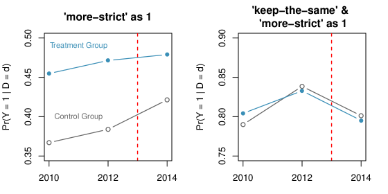
After transforming the outcome, scholars can check if the pre-treatment trends are parallel for this new binary variable. Inspecting pre-treatment trends is a routine often used in empirical studies to justify the use of the DID design (Angrist and Pischke, 2008). Figure 1 shows trends for each transformed outcome using the three-wave panel of the survey where I subset respondents who are not treated until 2012. The panel on the left shows the first type of transformation where only more-strict category is coded as (denoted by on the y-axis). We can see that the pre-treatment trends between the treatment group (blue) and the control group (gray) appears to be parallel (denoted by on the y-axis.). Thus if a researcher transforms the original variable in this way, she might conclude that the DID design is suitable for analyzing the data. The panel on the right shows the pre-treatment trends for the second type of transformation. In this case, however, the pre-treatment trends do not seem to be parallel: the trends cross during the pre-treatment period.
Note that this observation is not specific to this application. In Appendix C, I demonstrate that it is trivial to construct an example that satisfying parallel trends in one transformation does not imply the parallel trends in another transformation.
It is often unclear ex ante which threshold should be chosen from a substantive point of view. Therefore, it is unfortunate that the validity of the design appearently depends on how the variable is transformed. Although the running example only has three categories, the problem exacerbates when scholars need to analyze an outcome that has a larger number of categories.
3 The Proposed Methodology
3.1 The setup
Let denote the observed outcome measured on an ordinal scale with categories () for unit and time . The binary treatment, denoted by , is assigned after is observed but before time . We use the potential outcome notation to denote the counterfactual outcome, for . For example, is an attitude toward gun control regulations that would realize in the post-period if a respondent did not experience a mass shooting (i.e., the control condition).
In many applications, scholars are interested in estimating the distributional treatment effect. In this paper, I focus on the treatment effect on the treated. Specifically, the effect is defined as the difference in probabilities of choosing category under two conditions,
| (3.1) |
for . In our application, is the difference in probabilities that those treated prefer more strict gun control between the treated and the control conditions. Thus, observing implies that the mass shootings make people prefer stricter policies on gun control. Similarly, is the effect of the treatment on less-strict category and implies that incidents turn people to prefer less strict regulations.
When the number of categories is large, it is sometimes useful to estimate the cumulative effect , which is defined as a difference in probabilities of choosing or larger categories under the two conditions,
| (3.2) |
for . Note that by construction, and thus it is sufficient to consider the identification of .
The cumulative effect is also useful to connect the approach that dichotomizes ordinal outcomes to the proposed method. From the above definition, we can see that the standard DID based on the dichotomized outcome at threshold identifies . This is because where is the dichotomized potential outcome with threshold . This means that the standard DID applied to the dichotomized outcome can estimate only one of possible quantities of interest. Furthermore, if one wishes to estimate all possible ’s by changing the threshold, it requires distinct identification assumptions. As we saw in our motivating example, however, satisfying the parallel trends assumption for does not necessarily imply that the assumption for is satisfied.
3.2 Identification
Typically, we do not have a good sense of which estimand is best suited for answering the substantive question. Therefore, it is natural that we attempt to identify and estimate for all from the observed data. The goal of this section is to establish the identification of with a single set of assumptions.
To compute the quantity defined in Equation (3.1), we need the marginal distribution of and for the treated. While we observe for because , we need to impose additional assumptions to identify the distribution of for . Following Athey and Imbens (2006), I omit the subscript for units and denote where indicates and are equivalent in distribution. denotes the potential outcome under the control condition at time for group defined by . While we observe , and , the counterfactual outcome is what we do not observe in the data. In our example, is the potential attitude to gun control that we would have observed if those respondents who have experienced mass shootings would have not been exposed to the event.
I first impose a structure on the potential outcome. Specifically, I assume that the observed categorical outcome follows the index model, which means that there is a latent variable behind and that the categorical outcome is defined by a simple thresholding rule on the latent variable.
Assumption 1 (Index model).
Assume that the potential outcomes follow the index model such that there exists a latent variable and
| (3.3) |
where are a set of cutoffs with and .
Assumption 1 says that the potential outcome defined on an ordinal scale is a function of another potential outcome defined on a continuous space . In the application, can be considered as the underlying intensity of one’s attitude toward gun control policies where larger value of corresponds to a support for stricter gun control. The assumption allows us to handle the outcome on a continuous space through instead of directly working on a discrete space. Note that ’s are constants assumed to be fixed and they do not depend on group () nor time ().
Different from the additive effect, the distributional treatment effect requires that the entire marginal distribution of the potential outcome is identified. For that, I further impose a distributional assumption on in Assumption 2.
Assumption 2 (Location-scale family assumption).
Let denote a continuously distributed random variable with mean and variance that belongs to a parametric family. We assume that belongs to the location-scale family, that is, it can be written as
| (3.4) |
where is the location and is the scale parameter.
Assumption 2 specifies the distribution of the latent utilities. It assumes that each marginal distribution belongs to the location-scale family distribution with time and group specific location and scale parameter. This implies that the distribution of the potential outcomes are different up to mean and the scale. Note that the joint distribution of the latent utilities are left unspecified, so units can have correlated latent utilities over time. Although this is a parametric assumption (i.e., the distribution of should be known), the location-scale family encompasses a large class of parametric distributions (e.g., the normal distribution, the logistic distribution or the t-distribution, etc).
Finally, I impose a structure on the relationship between latent variables . This allows us to map what we observe in the control group over time to what would have happened to the treated group if it was not treated. I first start with a restrictive assumption that is similar to the standard DID design. It is possible to assume that the parallel trends hold on the latent outcome, that is,
| (3.5) |
Then, the mean of the counterfactual latent outcome is uniquely identified as
However, this approach is restrictive, because it requires an additional assumption that the variance is constant across time and groups, that is, for all and ; otherwise we cannot identify the entire distribution of the latent outcome . This constant variance assumption is strong because it only allows the unidirectional change of choice probabilities.
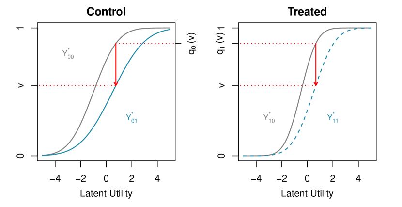
Therefore, I impose a different assumption from the standard parallel trends assumption. Instead assuming the mean shift, the assumption is imposed on the entire distributions, which is originally introduced by Athey and Imbens (2006) (also see Sofer et al., 2016). Specifically, I assume that the shift in the distribution across time are constant between the treatment and the control groups. Figure 2 graphically illustrates the assumption. The key part of this assumption is that the vertical arrows in the two graphs should be the same length. In other words, captures the trend in the distribution (i.e., how much “shifts” between and ) and the assumption says that the “shift” is identical across two groups. This means that for each choice of , the corresponding value of (“shift”) should be the same for .
Assumption 3 formally states the assumption.
Assumption 3 (Distributional parallel trends (Athey and Imbens, 2006)).
Let be the cumulative distribution function (CDF) of and define . Then, we assume that for all ,
| (3.6) |
Assumption 3 imposes a restriction on the relationship between the pre-treatment latent outcome and the counterfactual latent outcome , based on the relationship between two latent variables in the control group. Note that by construction for because CDFs should agree at the end of the support, .
Assumption 1, 2 and 3 identify the distribution of the counterfactual outcome. Proposition 1 presents the formal result.
Proposition 1 (Identification of the Counterfactual Distribution).
A proof is in Appendix A. Proposition 1 says that the location and the scale of the counterfactual latent outcome are uniquely determined by parameters of observed outcomes. This implies that we can recover the distribution of the counterfactual outcome (i.e., the potential outcome under the control condition for the treated unit at time ) using parameters estimated from the observed data, , and . For example, if we assume that follows the standard normal distribution, we have that follows the normal distribution with mean and variance .
3.3 Estimation
The identification result in the previous section provides a guidance on how we can estimate the causal effect from the observed data. Let denote a vector of parameters that characterize the distribution of the latent utility . I take a two-step approach to estimate causal quantity defined in Equation 3.1 for all . In the first step, I estimate parameters for observed outcomes, that is, , and . Based on the estimate of these parameters, causal effects are estimated in the second step.
In this and the following section, I focus on a case where follows the normal distribution, that is . Then, by Assumption 2, the observed outcomes , and follow the ordered probit model. Thus, parameters can be estimated via the maximum likelihood.
where is an indicator function that takes if the argument is true and takes otherwise, and is the cumulative distribution function of the standard normal distribution. Different from the standard ordered probit specification, I fix two cutoffs and (recall that and ). This allows us to estimate the variance component in addition to means (Lemma 1 in Appendix A; also see for example Jackman, 2009, Chapter 8). Note that the choice of is not consequential in that, the causal effect estimate is invariant to the choice of the cutoffs (Lemma 3 in Appendix A). This is because the identification assumption imposes a structure on the quantile scale, which is invariant to the scale of the latent variables, while different choices of cutoffs only affect the location and the scale (i.e., and ) of the latent variables.
We then estimate the parameter for the counterfactual distribution by the plug-in estimator based on the first stage,
| (3.8) |
Since the causal effect is a function of , the estimator for the causal effect is therefore given by
| (3.9) |
where , and then . Note that the first term of the right-hand side is a nonparametric estimator of because this quantity is identified from the data without any assumptions. The second term on the right-hand side is the counterfactual distribution identified by the assumptions (Proposition 1).
Lemma 4 in Appendix A establishes the consistency of the estimator , whose sampling variance can be derived using the delta method under the independence assumption. In practice, however, the block bootstrap can be used to estimate the variance when outcomes are correlated across time or due to clustering.
3.4 Assessing the distributional parallel trends assumption
In the standard DID design, additional pre-treatment periods provide an opportunity to assess the parallel trends assumption by checking the pre-treatment trends (Angrist and Pischke, 2008; Egami and Yamauchi, 2019). Although it is not a direct test of the assumption, observing the parallel trends in the pre-treatment periods suggests that the assumption is more likely to be plausible. With a similar logic, we can assess the validity of distributional parallel trends assumption (Assumption 3). Specifically, we would expect that if the distributional parallel trends holds for the pre-treatment periods, it is more reasonable to claim that the assumption holds in the post-period. Thus, we assess the validity of Assumption 3 by testing if the similar condition holds for the pre-treatment periods.
The proposed testing procedure
Suppose that we now observe the outcome for three time periods, , and where is the post-treatment outcome and and are the pre-treatment outcomes. The treatment is administered after time in this setup, and thus we have for regardless of the treatment status. This means that observed outcome before the treatment assignment is the same as the potential outcome under the control condition for both treatment and control groups.
Let denote the pre-treatment along of defined in Assumption 3, where I assume that . Recall that captures shift of distributions over time evaluated at quantile . The assumption requires that two functions are identical on the unit interval, that is, for all . Therefore, we wish to statistically test if holds for all using the data from the pre-treatment periods.
Intuitively, we can check the equivalence of two functions and by assessing the maximum deviation between two functions, . If this metric is “small”, we may conclude that . Formally, with some threshold , we wish to test the following hypotheses:
where says that two functions are not equivalent (i.e., large deviation). Rejecting the null implies that the data supports of equivalence which is what we want to demonstrate. For now, I assume that researchers know how to choose an appropriate value of based on substantive knowledge. I will discuss how to calibrate this equivalence threshold in the below. We can see that the null hypothesis can be written as a union of two hypotheses without absolute values, where
This decomposition implies that we can conduct two one-sided tests to determine if we reject the original null or not. In other words, we conclude that is false if we reject both and .
Now, suppose that we construct a % point-wise confidence interval for at each . The detail of how to construct the confidence interval is presented in Lemma 6 and 7 in Appendix A. Then, by the one-to-one relationship between the test and the confidence set, we reject if and only if the upper confidence interval is less than , that is
By the similar argument, we reject at level if and only if .
Proposition 2 shows that the proposed procedure is in fact asymptotically level test, that is, it rejects the null of non-equivalence with probability less than when the null is true.
Proposition 2 (Validity of the Testing Procedure).
For a given choice of the equivalence threshold and the level of a test , the testing procedure asymptotically controls the type I error, that is, under the null ,
as .
The above proposition shows that when the equivalence threshold is chosen such that the null is true (i.e., ), then the probably to falsely reject the null (type I error) is less than , for any value of that is consistent with the null. In other word, the proposed testing procedure is statistically valid for any choice of the equivalence threshold under the null.
The above result suggests that we can also compute the -value for this test by solving the rejection rule with respect to ,
where
Intuitively, the p-value for the test is the maximum of all point-wise -values because we are testing the maximum deviation of .
Choosing an equivalence threshold
So far, we have assumed that researchers have a clear idea what value should be used to assess the equivalence. When researcher have substantive knowledge about the appropriate value of given an application, it is reasonable to choose according to the knowledge. Oftentimes, this approach might not be feasible since it is not straightforward to form an idea of what value of should be deemed appropriate, especially when the value of is not directly tied to interpretable quantities such as causal effects. Although, any choice of is a valid choice because type I error is controlled for the corresponding null hypothesis, it seems useful to suggest a reasonable default value of to facilitate the practical use of the method.
I suggest the following value of as a reasonable starting point,
where with and when . This is a threshold used in the conventional KS test which is a nonparametric test on the difference between two distribution functions. The test is based on the maximum difference between two cumulative distribution functions. In KS test, the value of by the level of a test, but it is fixed here. The key feature of this threshold is that depends on the sample size. The equivalence threshold that depends on the sample size is discussed in Romano (2005). Intuitively, this selection of implies that we raise the standard of what the equivalence means as the sample size increases. Therefore, rejecting the null with larger will be a stronger evidence for the identification assumption.
4 Empirical Findings
In this section, I revisit the empirical application introduced in Section 2. We first reanalyze the two-wave panel of CCES (2010–2012). This two-wave panel is the data used for main analyses in the original studies. We then analyze the three-wave panel of CCES (2010–2012–2014) which allows us to assess the identification assumption using the pre-treatment periods.
In the following, we focus on estimating the following causal quantities:
for . Recall that less-strict is coded as 0, and more-strict category is coded as 2.
4.1 Result from the two-wave panel
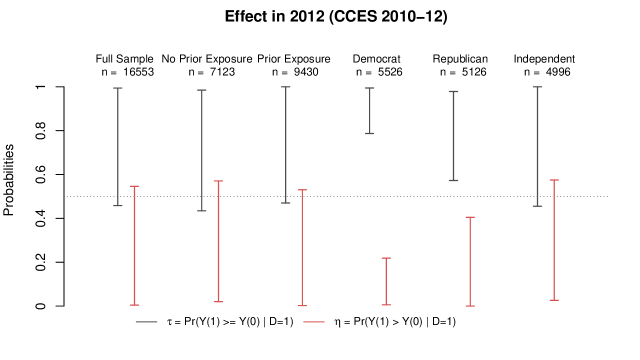
This section presents a result of the analysis on the two-wave sample from CCES (). The outcome is measured in 2010 and 2012 and I treat a response in 2012 as the post-treatment outcome. Respondents living in a neighborhood where mass shootings happened within 100 miles between 2010 and 2012 are considered as treated . In total, there were 16 mass shooting incidents recorded in the dataset between the two waves of CCES (Newman and Hartman, 2019, Appendix C). In addition to the analysis with the full sample, I also investigate effect heterogeneity by pre-treatment covariates. First, I investigate if the baseline safety of the neighborhood affects how people respond to mass shootings. Respondents are classified into either “prior exposure” group or “no prior exposure” group. A respondent is in the “no prior exposure” group if she is living in a neighborhood that did not have mass shootings within 100 miles of the area for the last ten years (as of 2010). We would expect that people react differently to mass shootings depending on how frequent these events are in their life. Second, following the original papers, I investigate if effects vary across respondents’ party affiliations. Since issues related to gun control are debated along the party line in the US, we might expect that people react differently depending on which party they affiliate with.
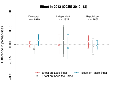
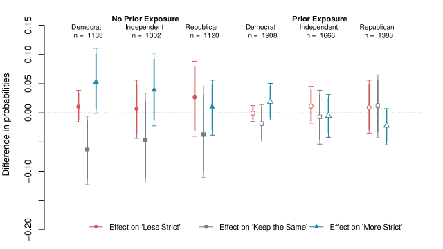
Figure 3 shows the results. In the figure, circles represent point estimates for which can be interpreted as the causal effect on preferring less strict gun regulations, while triangles shows estimates for which captures the effect on preferring more strict control of firearm sales; squares are estimate for the middle category (), which can be interpreted as a preference to the status quo.
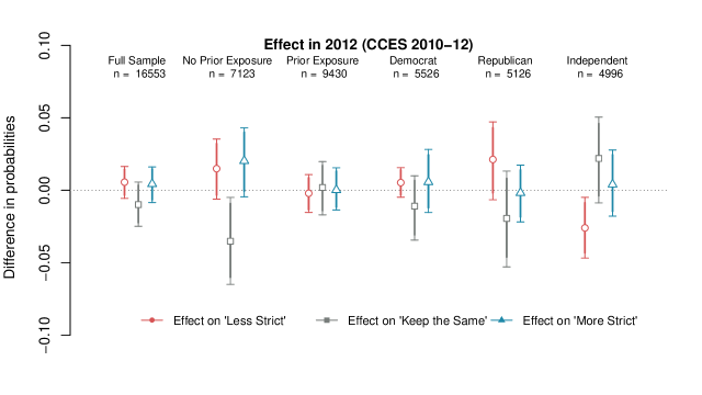
Along with point estimates, I also show the uncertain estimates. Thick (thin) vertical lines show 90% (95%) confidence intervals calculated via block bootstraps. To account for the fact that the treatment assignment is at the zip code level, the bootstrap is conducted blocking at the zip code level. There are unique zip codes in the two-wave sample. I sample zip codes with replacement and create bootstrap samples. Confidence intervals are based on bootstrap iterations. Text labels shown above estimates indicate the subsamples and their sample sizes used for the analysis.
We can see that causal effect estimates are not statistically significant at the 10% level for all categories in the full sample. Estimates are precisely estimated and they are all close to zero, indicating that there is little evidence to suggest that mass shootings have, on average, any effect on the attitude towards gun control regulations among those who live in their vicinity of public shootings.
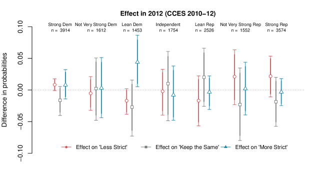
Following the original authors, I conduct two sets of subgroup analysis by “prior exposure” status and by the partisanship. The analysis reveals a similar pattern that most of the estimates are not statistically distinguishable from zero at the conventional level. However, we can also see that heterogeneity exists: the “no prior exposure” group has negative effect for the middle category (, ) which is statistically significant at the 5% level. This result implies that those living in the safer neighborhood (i.e., “no prior exposure”) move away from the status quo. Although not statistically significant at the 10% level, we can also see that the effect on the less strict category is positively estimated for this “no prior exposure” group, indicating that the shift away from the status quo was probably not uni-directional. We can also see the negative effect on less-strict category among the independents (, ), which is statistically distinguishable from zero at the 5% level. In Appendix D, I present a result using a more granular measure of partisanship used in the survey, which asks respondents to categorize themselves on a 7-point scale from “strong Democrat” to “Strong Republican.” The result in Figure D.1 shows that the effect is concentrated among lean Democrats, 91% of them categorized themselves as “independent” on the 3-point partisanship scale.
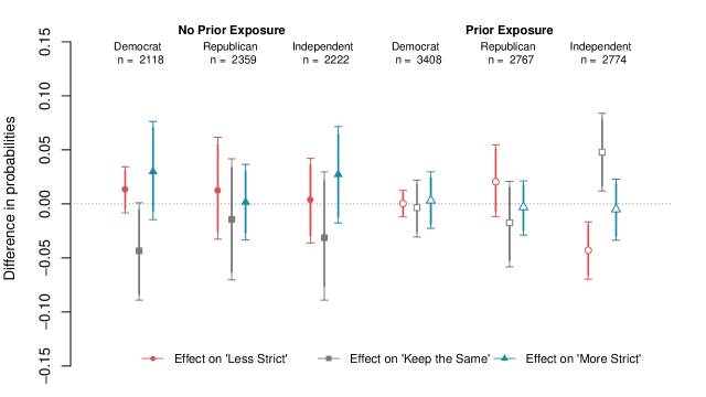
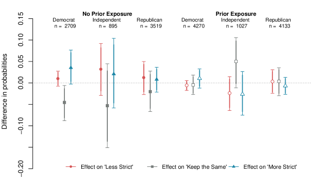
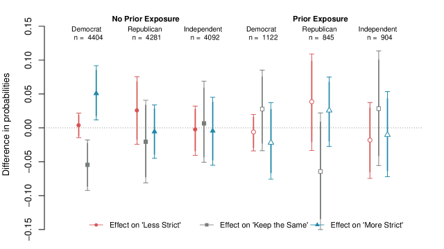
To further investigate the interactive effects between the the partisanship and prior exposure status, I considered interactions between the two variables. Figure 4 shows the results of the analysis. As we can see the effect is concentrated among Democrats who are in the “no prior exposure” group, while none of the effects are statistically significant for other partisans. The figure also shows that partisanship does not play a role in the “prior exposure” group where estimates are indistinguishable from zero.
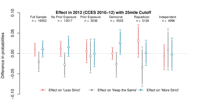
Finally, Barney and Schaffner (2019) consider different thresholds to determine who are “exposed” to the mass shootings. In addition to the above 100 mile threshold, I also estimate effects for the 25 mile threshold. The result is shown in Figure D.4 in Appendix D. We observe similar patterns with the previous results, while there are two notable differences. First, is now statistically significant at the 10% level (, ). Second, effects are clearer for Democrats without prior exposure: and and both of the estimates are statistically significant at the 5% level.
4.2 Diagnostics using three-wave panel
Next, I analyze the three-wave panel from CCES (2010-12-14) to assess if the identification assumption made in Assumption 3 is plausible or not. I subset the dataset so that I include only two types of respondents: those who experienced the mass shootings only after 2012 (treated group) and those who never experience the mass shootings throughout the sample periods (control group). This allows us to treat 2010 and 2012 as the pre-treatment periods, because no one in this subsample is affected by the treatment happened before 2012. To avoid the possibility that the past exposure might affect the baseline attitudes, I further condition on the prior-exposure variable, including only respondents who are in the “no prior exposure” group. This subset consists of respondents among which respondents are eventually treated between 2012 and 2014. In total, there were 28 incidents of mass shootings recorded in the dataset that happened between 2012 and 2014 waves.
I apply the diagnostic test proposed in Section 3.4 to the pre-treatment outcome. The goal here is to statistically test if the condition of the distributional parallel trend holds, namely, where is the pre-treatment analog of the quantile-quantile relationship defined on group (i.e., in Assumption 3). Specifically, I test the null hypothesis of non-equivalence, for all against the equivalence.
I compute the test statistic , where , and corresponding confidence intervals at the 5% level. Each is computed by evaluating and on the finite number of grid points between and where the distance between points is set to . The equivalence threshold is chosen based on the heuristic criterion discussed in Section 3.4, where and .
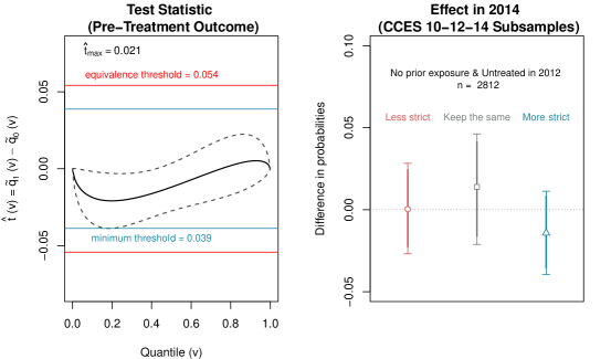
The left panel of Figure 5 shows the difference between the two functions, , evaluated at a value on the unit interval (solid line). Dashed lines show the point-wise 95% confidence intervals. The test statistic (the estimated largest deviation) is with the largest upper bound and the smallest lower bound . Since the confidence range is strictly contained in the equivalence range , we can reject the null of non-equivalence at the 5% level (). In other words, for any choice of that is greater than , we reject the null at the 5% level. The result suggests that during the pre-treatment periods the data supports the analogous condition of Assumption 3.
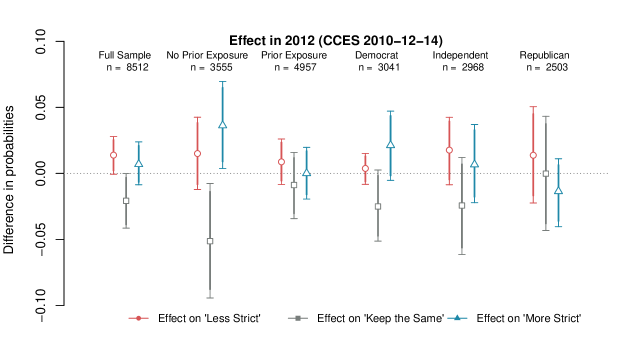
After confirming the plausibility of the key identification assumption, we now analyze the outcome measured in 2012 (pre-treatment) and 2014 (post-treatment) to estimate the causal effect for the three-wave subsample. The right panel of Figure 5 shows the result of the analysis. We can see that none of the estimates are statistically distinguishable from zero at the 10% level (, ; , ; and , ). This result somewhat contradicts findings in the previous section, where I found a negative effect on among the “no prior exposure” group. There are many possible reasons why effects could vary over time. One possibility is simply the size of the dataset. The subset of the three-wave panel has smaller respondents than the two-wave samples analyzed in the previous section. This difference obviously translates into differences in uncertainty estimates. Another possibility is due to the contextual differences. On December 14th, after the 2012 wave of the CCES, the Sandy Hook Elementary School shooting occured. This was one of the deadliest mass shootings in the US history, which possibly raised the salience of the issue affecting gun control regulations nationally.
5 Concluding Remarks
In spite of the recent developments in the literature on the DID design, less attention has been paid for when the outcome is measured on an ordinal scale. In this paper, I proposed a method that allows scholars to leverage ordinal outcomes without making the linearity assumption as in the the standard DID analysis. I also proposed a procedure that assesses if the key identification assumption is plausible when additional pre-treatment periods are available. This enable scholars to inspect the data and to discuss if the assumption is reasonable given a particular dataset they analyze, which is a crucial step for any research that attempts to establish a causal relationship.
Several extensions of the proposed methods are possible. In Appendix B, I demonstrate that the proposed method can be useful to estimate other types of causal estimands such as the proportion of who benefits from the treatment (e.g. Lu, Ding and Dasgupta, 2018). Recent years, it has been argued that such estimands are preferable because the distributional treatment effects considered in the main text are not necessarily easy to interpret. Because the proposed method identifies the entire distributions of the potential outcomes, it is possible to compute any causal estimand that is a function of marginal distributions of the potential outcome. In the appendix, I also discuss how to incorporate time-varying covariates, which requires a further modeling assumption.
In Appendix F, I present a simulation study where I assess the finite sample property of the proposed estimator and the testing procedure. I find that under the correct model specification, the proposed method outperforms the two competing methods: the standard difference-in-differences on the dichotomized outcome and the ordered probit model. I also find that the type-I error is properly controlled for the proposed testing procedure, while the power depends on the choice of the equivalence threshold.
Finally, future research should consider an extension to a complex design. Specifically, the staggered adoption design where the treatment is assigned over time is a popular data structure in applied studies. Although the development of such methods is beyond the scope of this paper, the same framework should improve the analysis of ordinal outcome beyond the standard DID setting.
References
- (1)
- Abadie (2005) Abadie, Alberto. 2005. “Semiparametric difference-in-differences estimators.” The Review of Economic Studies 72(1):1–19.
- Angrist and Pischke (2008) Angrist, Joshua D and Jörn-Steffen Pischke. 2008. Mostly harmless econometrics: An empiricist’s companion. Princeton University Press.
- Arkhangelsky et al. (2018) Arkhangelsky, Dmitry, Susan Athey, David A Hirshberg, Guido W Imbens and Stefan Wager. 2018. “Synthetic Difference in Differences.” arXiv preprint arXiv:1812.09970 .
- Athey and Imbens (2006) Athey, Susan and Guido W Imbens. 2006. “Identification and inference in nonlinear difference-in-differences models.” Econometrica 74(2):431–497.
- Barney and Schaffner (2019) Barney, David J and Brian F Schaffner. 2019. “Reexamining the Effect of Mass Shootings on Public Support for Gun Control.” British Journal of Political Science 49(4):1555–1565.
- Callaway and Sant’Anna (2018) Callaway, Brantly and Pedro HC Sant’Anna. 2018. “Difference-in-differences with multiple time periods and an application on the minimum wage and employment.” arXiv preprint arXiv:1803.09015 .
- Callaway, Li and Oka (2018) Callaway, Brantly, Tong Li and Tatsushi Oka. 2018. “Quantile treatment effects in difference in differences models under dependence restrictions and with only two time periods.” Journal of Econometrics 206(2):395–413.
- Card and Krueger (1994) Card, D and AB Krueger. 1994. “Minimum wages and employment: a case study of the fast-food industry in New Jersey and Pennsylvania.” American Economic Review 84(4):772–793.
- Chiba (2017) Chiba, Yasutaka. 2017. “Sharp nonparametric bounds and randomization inference for treatment effects on an ordinal outcome.” Statistics in Medicine 36(25):3966–3975.
-
Egami and Yamauchi (2019)
Egami, Naoki and Soichiro Yamauchi. 2019.
“How to improve the difference-in-differences design with multiple
pre-treatment periods.” Working Paper .
https://soichiroy.github.io/files/papers/double_did.pdf - Frymer and Grumbach (2020) Frymer, Paul and Jacob M Grumbach. 2020. “Labor unions and white racial politics.” American Journal of Political Science .
- Gay (2002) Gay, Claudine. 2002. “Spirals of trust? The effect of descriptive representation on the relationship between citizens and their government.” American Journal of Political Science pp. 717–732.
- Glynn and Ichino (2019) Glynn, Adam and Nahomi Ichino. 2019. “Generalized Nonlinear Difference-in-Difference-in-Differences.” Working Paper .
- Grose, Malhotra and Van Houweling (2015) Grose, Christian R, Neil Malhotra and Robert Parks Van Houweling. 2015. “Explaining explanations: How legislators explain their policy positions and how citizens react.” American Journal of Political Science 59(3):724–743.
- Hartman and Newman (2019) Hartman, Todd K and Benjamin J Newman. 2019. “Accounting for Pre-Treatment Exposure in Panel Data: Re-Estimating the Effect of Mass Public Shootings.” British Journal of Political Science 49(4):1567–1576.
- Jackman (2009) Jackman, Simon. 2009. Bayesian analysis for the social sciences. John Wiley & Sons.
- Jessee (2016) Jessee, Stephen. 2016. “(How) can we estimate the ideology of citizens and political elites on the same scale?” American Journal of Political Science 60(4):1108–1124.
-
Kuriwaki (2018)
Kuriwaki, Shiro. 2018.
“Cumulative CCES Common Content (2006-2018).”.
https://doi.org/10.7910/DVN/II2DB6 - Lechner et al. (2011) Lechner, Michael et al. 2011. “The estimation of causal effects by difference-in-difference methods.” Foundations and Trends® in Econometrics 4(3):165–224.
- Lee (2016) Lee, Myoung-jae. 2016. “Generalized difference in differences with panel data and least squares estimator.” Sociological Methods & Research 45(1):134–157.
- Li (2019) Li, Fan. 2019. “Double-Robust Estimation in Difference-in-Differences with an Application to Traffic Safety Evaluation.” arXiv preprint arXiv:1901.02152 .
- Likert (1932) Likert, Rensis. 1932. “A technique for the measurement of attitudes.” Archives of Psychology pp. 44–53.
- Liu et al. (2009) Liu, W, F Bretz, AJ Hayter and HP Wynn. 2009. “Assessing nonsuperiority, noninferiority, or equivalence when comparing two regression models over a restricted covariate region.” Biometrics 65(4):1279–1287.
- Lu, Nie and Wager (2019) Lu, Chen, Xinkun Nie and Stefan Wager. 2019. “Robust Nonparametric Difference-in-Differences Estimation.” arXiv preprint arXiv:1905.11622 .
- Lu (2018) Lu, Jiannan. 2018. “On the partial identification of a new causal measure for ordinal outcomes.” Statistics & Probability Letters 137:1–7.
- Lu, Ding and Dasgupta (2018) Lu, Jiannan, Peng Ding and Tirthankar Dasgupta. 2018. “Treatment effects on ordinal outcomes: Causal estimands and sharp bounds.” Journal of Educational and Behavioral Statistics 43(5):540–567.
- Mason (2015) Mason, Lilliana. 2015. ““I disrespectfully agree”: The differential effects of partisan sorting on social and issue polarization.” American Journal of Political Science 59(1):128–145.
- Newey and McFadden (1994) Newey, Whitney K and Daniel McFadden. 1994. “Large sample estimation and hypothesis testing.” Handbook of Econometrics 4:2111–2245.
- Newman and Hartman (2019) Newman, Benjamin J and Todd K Hartman. 2019. “Mass shootings and public support for gun control.” British Journal of Political Science 49(4):1527–1553.
- Qin and Zhang (2008) Qin, Jing and Biao Zhang. 2008. “Empirical-likelihood-based difference-in-differences estimators.” Journal of the Royal Statistical Society: Series B (Statistical Methodology) 70(2):329–349.
- Romano (2005) Romano, Joseph P. 2005. “Optimal testing of equivalence hypotheses.” The Annals of Statistics 33(3):1036–1047.
-
Schaffner and Ansolabehere (2015)
Schaffner, Brian and Stephen Ansolabehere. 2015.
“2010-2014 Cooperative Congressional Election Study Panel
Survey.”.
https://doi.org/10.7910/DVN/TOE8I1 - Sofer et al. (2016) Sofer, Tamar, David B Richardson, Elena Colicino, Joel Schwartz and Eric J Tchetgen Tchetgen. 2016. “On negative outcome control of unobserved confounding as a generalization of difference-in-differences.” Statistical Science 31(3):348.
- Volfovsky, Airoldi and Rubin (2015) Volfovsky, Alexander, Edoardo M Airoldi and Donald B Rubin. 2015. “Causal inference for ordinal outcomes.” arXiv preprint arXiv:1501.01234 .
Appendix
Appendix A Proofs of Propositions
A.1 Lemmas
Before proving propositions, we present useful lemmas.
Lemma 1 (Identification of mean and variance of the latent variables.).
Suppose that the cutoffs are fixed at and for . Then, and in are uniquely identified from the observed probability distribution.
Proof of Lemma 1.
Suppose that has the density . Then, we can form a non-linear system of equations
which are sufficient for estimating and . ∎
Lemma 2 (Alternative formula for identification).
Proof of Lemma 2.
Under the distributional parallel trends assumption, we have for all . Then,
where the first equality is due to the definition of and the last equality follows by Assumption 2. Pick and as in the statement. Drawing on a similar to the argument in Lemma 1, we obtain the identification.
∎
Lemma 3 (Invariance of under different cutoffs).
Suppose we have two sets of cutoffs and () for . Then, .
Proof of Lemma 3.
Let denote the cumulative distribution function of the latent variable under the cutoff . Similarly, let denote the CDF under . To show the causal effect estimates are invariant to the choice of cutoffs, it is sufficient to show that , that is, the invariance of the identified counterfactual latent distribution.
We first show that for and . Now, note that we have because
where is the observed outcome. Thus,
which proves that .
Next, by the similar argument, we have that , because
Repeating the above two steps for and , we obtain that
and
where and .
Applying the result of Lemma 2, we can see that and are uniquely identified under different sets of cutoffs, that is, .
Finally, replacing all quantities with their sample analog, we conclude that . ∎
Lemma 4 (Asymptotic Normality of Causal Estimates).
Under some regularity conditions, as with , we have that
| (A.1) |
Proof of Lemma 4.
We prove the statement by showing the following two statements:
-
1.
is -consistent estimator for .
-
2.
is -consistent estimator for .
We then use the continuous mapping theorem for the convergence in distribution to obtain the final result.
To be clear, we (sometime implicitly) condition on throughout the proof, which assumes that there is a super population of units with . Now let and . Under the assumption that for any combination of and , it follows that as with by the law of large numbers. This proves the consistency. By the central limit theorem, it also follows that
as with .
Next, recall that is given as a transformation of , and , all of which are MLE of the problem described in Section 3.3. Therefore, under the assumption of correct model specification, we obtain that , and are jontly asymptotically normal centered around , and . By the continuous mapping theorem, it follows that is also asymptotically normally distributed.
Finally, using the continuous mapping theorem again, we have that is a consistent estimator for where the variance is obtained by the delta method (See Lemma 6).
∎
Lemma 5 (Asymptotic Normality of for Pre-treatment Parameters).
Let , all of which are estimated using the data from the pre-treatment periods. Then, under regularity conditions in Newey and McFadden (1994), the maximum likelihood estimator is asymptotically normal with covariance ,
| (A.2) |
where is a block-diagonal matrix under independence assumption.
Proof of Lemma 5.
The result is a direct application of the standard result of the maximum likelihood estimation. Therefore, proof is omitted. ∎
Lemma 6 (Asymptotic Distribution of the Test Statistic).
Assume that . Let and . Then, we have that
| (A.3) |
for each with
| (A.4) |
where is evaluated at the truth, is the asymptotic variance covariance matrix of given in Lemma 5, and the gradient takes the form of
with
Proof of Lemma 6.
Recall that the derivative of the error function is given by
| (A.5) |
which is differentiable with respect to .
Now, I compute the derivative of with respect to ,
where
Given that Lemma 5 establishes the asymptotic normality of , the result immediately follows by the application of the Delta method. Then, we get
| (A.6) |
From here, we obtain the variance formula as
where . ∎
Lemma 7 (Validity of ) level sets (Liu et al., 2009)).
Let . Suppose and are point-wise upper and lower level confidence intervals, respectively such that and . Then,
| (A.7) | ||||
| (A.8) |
Proof of Lemma 7.
Recall that is a point-wise % level confidence interval. This implies that
for any . Now, let . Then, we have that
which proves that .
∎
A.2 Proofs
Proof of Proposition 1.
Let denote a random variable with mean and variance and denote its cumulative distribution function by . For , we have
The equality in the above expression holds because follows the location-scale family, which implies
Combined with the fact that is a continuous and parametric distribution, we recovers the distribution of .
∎
Proof of Proposition 2.
Case 1: . In this case, the test makes a “mistake” because the upper bound does not cover . Thus, we can focus on an event . Since , we can bound as
| (A.9) |
Now, consider a particular value of . Then, we have that
where the last inequality uses the fact that asymptotically is a level confidence interval (Lemma 7).
Case 2: . In this case, we focus on the other event . Since , we have that
where the last inequality is a direct application of Lemma 7. ∎
Appendix B Extensions
B.1 Other estimands
This section provides an extension of the proposed methodology. Following the recent developments in the literature on causal inference with ordinal outcome, where more interpretable estimands have been proposed, I show how to apply the proposed method to those new estimands.
In the above section, we have focused on particular causal estimands, and , which is a difference in probabilities defined for a specific reference category . One issue of this quantity is that depending on the choice of reference category , the sign of the estimate might flip. This means that interpretation becomes tricky because it is completely possible to observe and for with the same data. From this, we cannot even conclude that the treatment had “positive” effect or not.
To circumvent this problem associated with , recent papers turn to different kinds of estimands for ordinal outcome (e.g., Volfovsky, Airoldi and Rubin, 2015; Chiba, 2017; Lu, Ding and Dasgupta, 2018; Lu, 2018). For example, Lu, Ding and Dasgupta (2018) considers the following estimand:
| (B.1) |
This is a proportion units of who benefit from (or at least not harmed by) the treatment. In our example, captures the proportion of treated respondents who change their opinion toward gun control (regardless of their baseline attitudes) after experiencing the mass shooting in their neighborhood. This quantity is easy to interpret because it does not depend on the baseline attitude and smaller value of indicates that there are few respondents who change their opinion towards gun controls. However, since depends on the joint distribution of potential outcomes, , it cannot be point identified. Lu, Ding and Dasgupta (2018) provides a closed form bound for this estimand using only the marginal distribution of and .
The benefit of the proposed method over the dichotomizing-the-outcome approach is that it identifies the entire distribution of , whereas the information about the entire distribution is lost when we use the coarsened outcome. This implies that we can estimate the bound based on given in Equation (3.8). Following the result of Lu, Ding and Dasgupta (2018), we can estimate the bound as
where is the estimate of the distributional effect, and by construction. We can see from the formula that the upper bound is informative as long as there is at least one reference category such that for . Otherwise, will be the minimum and thus we get the non-informative upper bound .
B.2 Time-varying covariates
Researchers might want to incorporate time-varying covariates into the analysis to further gain efficiency. I discuss that the parametric specification of the proposed method allows the use of such covariates for analysis. Although sometimes appealing, I emphasize that parametric specification introduces additional assumptions for the analysis.
Let denote a dimensional vector of time varying covariates. We can model the mean and the variance of the latent utilities as
where . Then, we can express the observed choice probability as
We estimate parameters by the maximum likelihood.
Finally, the quantities of interest is estimated by taking the sample average of predicted probabilities.
Note that the marginalization of covariates is with respect to the distribution for the treated, because our estimand is defined for the treated units.
Appendix C Dichotomizing the Outcome: An Example
Coarsening the ordinal outcome into a binary variable is a common practice often employed in applied works. Although this procedure allows scholars to utilize the standard linear DID, I will demonstrate in this section that this operation leads to an inconsistent result depending on how the new variable is created.
To see this, let’s consider a simple example with three categories, . There are two possible ways to transform this variable into a binary outcome, or . Under this setup, we require two separate parallel trends assumptions for identification,
PT1 identifies and PT2 identifies . Also let be the conditional probability for the potential outcome under the control.
Now consider the following data generating process which specifies the marginal distributions for the potential outcome:
Under this DGP, PT1 holds since
However, PT2 does not hold because
Thus, this example demonstrate that with the same data, can be consistently estimated with but cannot be estimated without bias, even though we have the same data generating process behind the two transformations. Obviously, it is also trivial to construct an example where PT2 holds but PT1 does not.
Appendix D Additional Empirical Results
D.1 Different coding of partisanship
Given the partisan nature of the gun control policies, it is important to understand if the effect of mass shootings could differ by respondents’ party identification. The coding of partisanship, however, slightly different across studies. In the main text, I relied on the 3-point scale party identification question (pid3), which asks respondents the following question,
Generally speaking, do you think of yourself as a ...?
(1) Democrat; (2) Republican; (3) Independent;
(4) Other; (5) Not sure; (8) Skipped.
In the analysis, I exclude respondents who do not select option (1), (2) or (3).
In the survey, respondents are also asked to place themselves on a granular scale of partisanship (pid7):
Would you call yourself a strong Democrat or a not very strong Democrat? Would you call yourself a strong Republican or a not very strong Republican? Do you think of yourself as closer to the Democratic or the Republican Party?
(1) Strong Democrat; (2) Not very strong Democrat; (3) Lean Democrat;
(4) Independent; (5) Lean Republican; (6) Not very strong Republican;
(7) Strong Republican; (8) Not sure; (98) Skipped.
Figure D.1 shows the result of the analyses that use pid7 to construct partisan subgroups. We can see that the effect is concentrated among “Lean Democrats.”
On the other hand, Barney and Schaffner (2019) constructs the partisanship variable based on pid7 but collapses it into a 3-point scale, “Democrat”, “Independent” and “Republican”. The major difference from the self-reported pid3 is that “leaners” are classified as partisans (i.e., not independents).
D.2 Different estimands
Figure D.3 shows estimated bounds on (gray lines) and (red lines). The explicit formula of the bound for each estimand is given in Section B.1.
I find that bounds for the two estimands diverge suggesting there are many observations that have in the population. For example, among Democrats, the bound for is between around 0.8 and 1.0 which might suggest that proportion of Democrats who supports gun control when treated is extremely high. However, the bound for is between around 0.2 and 0 which might suggest that proportion of Democrats who have strictly prefer a more strict gun control is very small. This is a problem discussed in Lu, Ding and Dasgupta (2018) where and cannot be informative when there are many units who does not change attitudes by the treatment. Therefore, it appears that we need to turn to other estimators that avoid this problem (e.g., Chiba, 2017; Lu, 2018).
D.3 Different treatment cutoff
Although Newman and Hartman (2019) define the exposure by the 100-mile cutoff, Barney and Schaffner (2019) consider different threshold to assess the robustness of the results. Following their analysis, I consider an alternative threshold of 25 miles. Figure D.4 shows the result. Note that the “prior exposure” is also defined by the 25-mile cutoff.
D.4 Two year subset of three-wave panel
In this section, I present two additional results based on the two-wave panel from CCES. Figure D.5 shows estimated effects based on the sub-group analysis taking interactions between the prior exposure variable and partisan identification. In the figure, circles (triangles) show estimates of () and thin (thick) line indicate 90% (95%) confidence intervals. Confidence intervals are computed based on block bootstraps (blocked at the zip code level).
I find that among no-prior-exposure group, the effect is concentrated among Democrats ( for Democrats is estimated positive and statistically different from zero at the 10% level, while is not statistically significant). On the other hand, effects for Independents and Republicans are both indistinguishable from zero at the 10% level (neither nor ). I also find that effects are almost zero in the prior-exposure groups regardless of partisanship.
Appendix E Details of the Application
A list of method used in the original studies
Table 1 summarizes the methods used in the original papers.
Coding of mass shootings
Newman and Hartman (2019) uses the following criteria to determine if an incident constitutes a mass public shooting: “(1) firearms as the primary weapon used, (2) attacks on non-family members of the general public and (3) attacks in which at least three or more individuals were injured or killed.” (Newman and Hartman, 2019, p.8). See the original studies for the detail of why these criteria are selected. Note that the definition of the “treatment” is slightly different between Newman and Hartman (2019) and Barney and Schaffner (2019). I follow the definition used by Barney and Schaffner (2019); Please see Barney and Schaffner (2019) for the discussion on this point.
Survey outcome
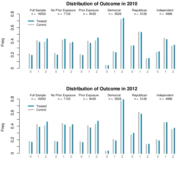
The ordering of the response categories is not exactly the same as the original question in CCES 2010–2012 panel. Originally in the survey, the choices are given as (1) More Strict; (2) Less Strict; (3) Kept As They Are (please see CC10_320 and CC12_320 in “Guide to the 2010-12 CCES Panel Study” available at https://doi.org/10.7910/DVN/24416/79YKV2). In the main text, I follow the coding of Newman and Hartman (2019) and Barney and Schaffner (2019) and treat “Kept As They Are” as the middle category.
Figure E.1 shows the distribution of the outcome in 2010 (top) and 2012 (bottom) where the blue bars correspond to the treatment group and the gray bars correspond to the control group.
Appendix F Simulation Studies
In this section, I present two Monte Carlo studies to investigate finite sample performances of the proposed method. The first simulation assesses performance of the proposed estimator for the causal effect where I compare the proposed estimator against the standard difference-in-differences with dichotomized outcome and the ordered probit regression. The result shows that the proposed estimator is unbiased to the causal effects and the confidence interval has nominal coverage, while the other two method are biased and thus the confidence intervals fail to maintain the coverage. The second simulation studies the finite sample performance of the proposed procedure for the diagnostic in Section 3.4. I demonstrate that the type I error is controlled under the range of equivalence threshold that is compatible with the null and that the power converges to one when the equivalence threshold is chosen reasonably.
F.1 Estimating causal effects
In this first simulation study, I investigate the finite sample performance of the proposed estimator under the correct model specification. The potential outcome is generated by first drawing the latent utilities from the normal distribution. For the potential outcome under the control, the following set of parameters are used to generate the data: , and . The parameters for the counterfactual outcome is set according to the identification formula in Proposition 1. The parameters for generating the potential outcome under the treatment, , are set as and .
After generating the latent utilizes, they are transformed into categorical outcome with categories based on the set of cutoffs. In this simulation, I consider and also I vary the number of units .
Since there are possible treatment effects to consider, that is, , estimators are evaluated on averaging the loss over treatment effect estimates. Specifically, I consider the following metrics:
where is the estimate of under th Monte Carlo iteration and is the % confidence interval for .
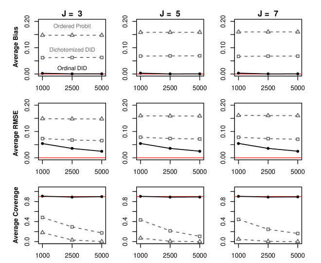
Figure F.1 shows the result. Left panel shows the absolute bias of the estimate. We see that the bias is larger when the sample is relatively small for as the number of observations in each category tend to be smaller. However, in general, estimates are unbiased. Middle panel shows the RMSE. It shows that RMSE decreases as the sample size increases and the variance is smaller when the number of categories are smaller. Finally, the right panel shows the coverage of 90% confidence intervals. We can see that for both cases, confidence intervals have nominal coverage regardless of sample size.
F.2 Testing procedure
In this section, I investigate a finite sample performance of the proposed testing procedure. Specifically, I conduct a Monte Carlo simulation with a scenario that Assumption 3 is violated in the pre-treatment periods. Outcomes are generated first by simulating the latent utilities. The latent utilities are simulated according to the normal distribution with mean and variance ,
| (F.1) |
I set , , and . This parameter specification leads to the true maximum deviation . Clearly, this does not satisfy Assumption 3 which requires .
After simulating , categorial outcomes are generated based on cutoffs . In this simulation, I consider three cases: . For and , the same cutoffs as in the previous simulation are used. For , I use .
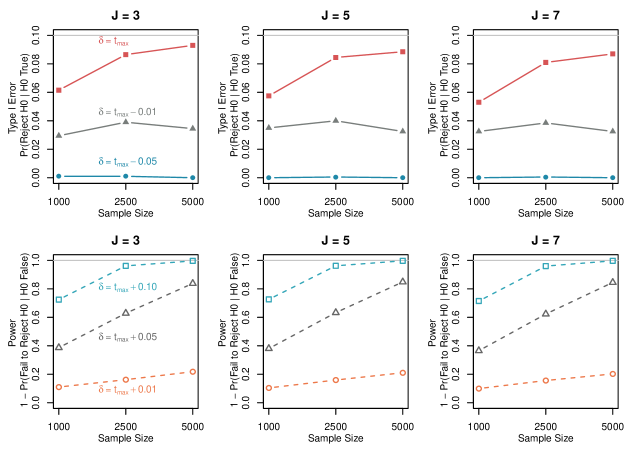
In order to assess how the test performs depending on a choice of equivalence thresholds, I vary . The value of is chosen such that in some range of , the null of is true and in other range of the null is false (i.e., ). For the range of that satisfies , I set . We would expect that the test is more likely to reject the alternative when . For the range of that does not satisfy , I set . Among them, we expect that the test can reject the null most likely when .
Figure F.2 shows the results for this simulation. The upper panels show type I errors when the choice of is consistent with the data (i.e., ). Recall that the data is simulated such that the equivalence does not hold. Thus, we would expect that the null, , is not rejected and the probability of falsely rejecting the null (type I error) should be less than . In fact, we can see that the proposed testing procedure controls the type I error. In addition, the smaller value of (i.e., a smaller rejection region for ) leads to lower type I error. The lower panels show results for type II errors when the choice of is not consistent with the data (i.e., is false). We can see that the test struggles to reject the null when is set to close to . When is set to a value far away from , type II error converges to zero as sample size increases.