Largo Bruno Pontecorvo, 3 - 56127 Pisa, Italy
22email: luca.gemignani@unipi.it 33institutetext: Lucia Romani, Alberto Viscardi 44institutetext: Dipartimento di Matematica, Alma Mater Studiorum Università di Bologna,
Piazza di Porta San Donato, 5 - 40126 Bologna, Italy
44email: lucia.romani@unibo.it, 44email: alberto.viscardi@unibo.it
Bezout-like polynomial equations associated with dual univariate interpolating subdivision schemes
Abstract
The algebraic characterization of dual univariate interpolating subdivision schemes is investigated. Specifically, we provide a constructive approach for finding dual univariate interpolating subdivision schemes based on the solutions of certain associated polynomial equations. The proposed approach also makes possible to identify conditions for the existence of the sought schemes.
Keywords:
Bezout equation; Univariate dual subdivision; Higher arity; InterpolationMSC:
65F05 68W30 65D05 65D171 Introduction
Subdivision schemes are useful tools for the fast generation of graphs of functions, smooth curves and surfaces by the application of iterative refinements to an initial set of discrete data. The major fields of application of subdivision schemes are Computer Graphics and Animation, Computer-Aided Geometric Design and Signal/Image Processing, but a further motivation for their study is also their close relation to multiresolution analysis and wavelets. The last connection was especially investigated in the case of interpolating subdivision schemes and it was pointed out that interpolatory subdivision schemes of Dubuc-Deslauriers MR982724 are connected to orthonormal wavelets of Daubechies CDbook ; Micchelli1996InterpolatorySS . Interpolating subdivision schemes were also deeply studied because considered very efficient in representing smooth curves and surfaces passing through a given set of points. In fact, after five or six subdivision iterations only, they are capable of providing the refined set of points needed to represent on the screen the desired smooth limit shape interpolating the given data. The main properties of interpolating subdivision schemes were investigated over the past 20 years by several researchers (see, e.g., DUBUC1986185 ; Dyn02 ; GAVHIMOLEFE2019354 ) and many approaches were proposed to design their refinement rules. However, as far as we are aware, before the papers LUCIA ; RV , no one ever tried to construct interpolating subdivision schemes that do not satisfy the stepwise interpolation property and are thus not defined via refinement rules that at each stage of the iteration leave the previous set of points unchanged. Stepwise interpolating subdivision schemes - also known as primal interpolating subdivision schemes MR982724 ; MR2008967 - are defined by finite subdivision masks of odd width that contain as a special submask the sequence . Differently, members of the most recently introduced class of non-stepwise interpolating subdivision schemes –also known as dual interpolating subdivision schemes– are characterized by finite masks with an even number of entries that do not necessarily contain as a special submask the sequence. One of the contributions of RV was to show that, under some suitable/auxiliary assumptions, the coefficients of the subdivision mask of a dual interpolating scheme can be (possibly) determined by the solution of an associated rectangular linear system. This system can be clearly inconsistent for some choices of input data and/or size (length) of the mask. For a given input data set the approach taken in RV consists of an exhaustive analysis of the associated linear systems of increasing sizes in order to identify possible consistent configurations.
In this paper we pursue a different method for constructing dual interpolating subdivision schemes based on the reduction of the matrix formulation into a functional setting to solving a certain Bezout-like polynomial equation. The method makes possible to address the consistency issues by detecting suitable conditions on the input data which guarantee the existence of a dual interpolating scheme. Additionally, it yields a full characterization of the set of solutions which can be exploited to fulfil additional demands and properties of the solution mask. From the point of view of applications, such a computational approach allows the user to meet specific requests in terms of polynomial reproduction, support size and regularity. Even though a general result concerning convergence and/or smoothness of a dual interpolating subdivision scheme is not yet available, in all the considered specific cases the analysis can be performed by using ad-hoc techniques. Illustrative examples and comparisons with existing primal interpolating schemes are provided and discussed.
2 Background and notation
In this section we briefly recall some needed background on subdivision schemes of arbitrary arity , .
Any linear, stationary subdivision scheme is identified by a refinement mask that is usually assumed to have finite support, i.e. to satisfy for for suitable .
The subdivision scheme identified by the mask consists of the subsequent application of the subdivision operator
which provides the linear rules determining the successive refinements of the initial sequence of discrete data . Introducing the notation , we can thus describe the subdivision scheme as an iterative method that at the -th step generates the refined scalar sequence
| (1) |
Attaching the data generated at the -th step to the parameter values with
(these are usually set as ) we see that the subdivision process generates denser and denser sequences of data so that a notion of convergence can be established by taking into account the piecewise linear function that interpolates the data, namely
where is the space of linear polynomials. If the sequence of the continuous functions converges uniformly, then we denote its limit by
and say that is the limit function of
the subdivision scheme based on the rule (1) for the data MR1079033 . When , is called basic limit function.
The analysis of convergence of a subdivision scheme can be accomplished by studying the properties of the so-called symbol of the subdivision mask MR1172120 .
The symbol of a finitely supported sequence is defined as the Laurent polynomial
Besides convergence and smoothness, many other properties of a subdivision scheme, like polynomial generation and reproduction, can be checked by investigating algebraic conditions on the subdivision symbol MR2775138 . While the term polynomial generation refers to the capability of the subdivision scheme of providing polynomials as limit functions, with polynomial reproduction we mean the capability of a subdivision scheme of reproducing in the limit exactly the same polynomial from which the data are sampled. The property of polynomial reproduction is very important since strictly connected to the approximation order of the subdivision scheme and to its regularity CHOI2006351 ; MR2474706 . With respect to the capability of reproducing polynomials up to a certain degree, the standard parametrization (corresponding to the choice , ) is not always the optimal one. Indeed, the choice with , turns out to be the recommended selection MR3071114 . The subdivision schemes for which are termed primal, whereas the ones for which are called dual. The target of this work are dual schemes. While dual approximating schemes were investigated extensively (see, e.g., MR3071114 ; DUBUC2011966 and references therein), to the best of our knowledge dual interpolating schemes were only considered in the recent papers LUCIA ; RV .
3 Basic reductions
The aim of this section is to investigate the algebraic characterization of univariate dual interpolating subdivision schemes of arity .
According to the results shown in RV , the construction of such schemes requires as input the desired degree of polynomial reproduction and some samples of the
resulting basic limit function . A similar procedure was investigated in DeVilliers2016759 ; MR1790328 , where the samples of
the basic limit function at the integers were required: here instead the samples at the integers are fixed to be the sequence and
information about the samples at the half-integers are required.
More specifically, in RV it is seen that taking Fourier transforms on both sides of the refinement equation for the basic limit function
allows one to describe
the mask of dual interpolatory schemes in a matrix setting in terms of the solution of certain bi-infinite Toeplitz-like linear systems
in banded form. In this paper we exploit the interplay between the functional and the matrix settings into more details. In particular, from the matrix setting we come back to
the functional one by relying upon the connection of Toeplitz-like systems with corresponding Bezout-like polynomial equations. This connection yields
a constructive approach to determine the associated symbols. Moreover, the proposed approach also makes possible to identify conditions
for the existence of the sought dual interpolatory schemes
In the following, to simplify the presentation, we distinguish between odd and even arity.
3.1 The odd arity case
Now let us consider the solution of the linear system in RV for the case where is an odd integer. The system is defined as follows:
| (2) |
where
and is a given fixed function. By suppressing zero rows in both and we obtain the equivalent linear system
| (3) |
where
The interplay between computations with polynomials and Toeplitz-like matrices can be exploited to recast the solution of the linear system (2) in terms of solving an associated Bezout-like polynomial equation. Indeed from the proof of Theorem 4.1 in RV one deduces that the entries of the unknown vector satisfy
| (4) |
which implies
| (5) |
The system (5) can be rewritten into a more compact form by using the decomposition of that involves the sub-symbols of the scheme given by
| (6) |
Let us introduce the corresponding decomposition of the Laurent polynomial defined by
| (7) |
The first equation of (5) determines . Then the second equation can be read as follows
or, equivalently,
| (8) |
Our computational task is therefore reduced to compute a Laurent polynomial defined as in (6) satisfying the Bezout-like polynomial equation (8). It is quite natural for convergence and reproducibility issues to impose some other constraints of the form
| (9) |
Our proposed construction of such a polynomial works under some additional assumptions on the input data encoded in the function . More specifically:
ASSUMPTION 1
: We suppose that for a certain the ring of Laurent polynomials in over .
ASSUMPTION 2
: We suppose that , , are relatively prime, i.e. they have no common zeros.
Under these assumptions our composite approach for computing proceeds by the following steps.
3.2 The proposed approach
The first step consists of determining the values , , . From (9) one gets immediately , . The first equation of (5) implies and, hence, from Assumption 1
| (10) |
This equation sets the values attained by the function and its derivatives at the point 1.
Theorem 3.1
If satisfies (10) then it holds
Proof
The remaining unknowns , , , , are computed by solving the linear system obtained by differentiation of (9). Specifically, by differentiating times the expression of in (6) with respect to the variable we find that
|
|
(11) |
where are polynomials defined by Hoppe’s formula for derivation of composite function according to
If , , are the -th roots of unity, then from (9) it follows that , , . In the view of (11) this implies that the values , , , , can be computed recursively by solving
with . The system can be expressed in matrix form as
|
|
(12) |
where
Here , , is the diagonal matrix with diagonal entries , , and is the Vandermonde matrix with nodes , . Since , , are distinct and non-zero, the coefficient matrix is nonsingular and , , , are uniquely determined.
Once the quantities , , , are calculated then the sub-symbols , , , can be represented as follows
| (13) |
for suitable . This representation is exploited in the second step to find a solution of (8). Let us introduce the truncated representation of the symbol , that is,
First of all, we notice that in the view of (8) the sub-symbols of the function should fulfil the compatibility relations obtained by differentiating (8) at the point . Specifically, by setting
we require that
The following result provides this compatibility for free.
Theorem 3.2
Proof
Let us consider the auxiliary function . From (10) it follows that . By construction satisfies relations (9). By using the representation of provided by (9) this gives
with . Observe that
and, hence,
|
|
(14) |
Moreover it can be easily seen that the two sets and coincide. Besides this, by direct multiplication of and , we can write
| (15) |
for suitable Laurent polynomials . Since the class of integers congruent to modulo is . It follows that , , is such that . Hence, by comparison of classes mod in (14) and (15), we obtain that
From (10) this implies that
which concludes the proof.
By setting
| (16) |
from Theorem 3.2 it follows that the polynomial corrections , , satisfy the Bezout equation
| (17) |
Under Assumption 2 this polynomial equation is solvable GS . In particular, following GS every solution of (17) can be written as
where
and is any element of . This general form of the solution can be exploited whenever we look for masks with additional properties. Of great importance for applications is the case where is required to be symmetric, that is, . The existence of a symmetric solution can be proved under the auxiliary assumption that , . In this case from (4) we obtain that is a solution if and only if is a solution, too. By linearity this implies that also determines a symmetric solution. If this solution is not of minimal length one can exploit the general form above to further compress the representation.
Example 1
Let us illustrate our composite approach for the odd case by means of a computational example. We choose , and
Thus, according to (7),
with
After solving the linear system (12), we have from (13)
with
and
To search for compatible and , we first compute
in such a way that (16) holds, i.e.,
Then we look for particular solutions and such that
A possible choice is
After symmetrization, the resulting mask is such that for .
To obtain a smaller symmetric mask, we search for a suitable so that replacing
in the previous expressions of and , leads to the final symbol
satisfying . The choice of that leads to the shortest mask is
and the first half of the resulting symmetric mask is
| (18) |
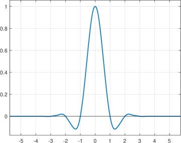
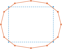
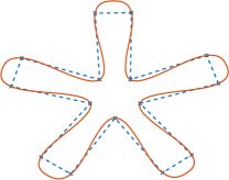
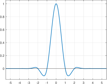
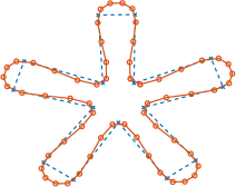
The basic limit function related to the mask in (18) is shown in Figure 1, and two examples of interpolating curves can be found in Figure 2. We have that and, via joint spectral radius techniques MR3886713 ; MR3009529 ; THOMAS2 , one can prove that . By construction the corresponding subdivision scheme reproduces polynomials of degree . On the other hand the primal interpolating ternary -point scheme (see, e.g., MR3702925 ) reproduces quintic polynomials as well but it has a basic limit function supported in .
3.3 The even arity case
Let us now consider the solution of the linear system in RV for the case where is an even integer. The system is defined as follows:
| (19) |
where
and is a given fixed function. By suppressing zero rows in both and we obtain the equivalent linear system
| (20) |
where
According to RV , (19) and (20) can be expressed in functional form as
which can be rewritten as
| (21) |
By Assumption 1 the right-hand side of (21) satisfies
Concerning the representation of the left-hand side of (21) let us introduce the modified subsymbols defined by
| (22) |
Notice that if , , denote the subsymbols of the mask of arity then we have
| (23) |
In particular this implies that
Moreover from and one deduces that
| (24) |
Then for the left-hand side of (21) it holds
Hence, it follows that relation (21) can be reformulated as the Bezout-like polynomial equation
| (25) |
From (23) it follows that the equation (25) can be rewritten in a more customary form as
Hereafter, let us assume that Assumption 2 holds for the subsymbols of the mask of arity . We also make the following further assumption.
ASSUMPTION 3
It is assumed that
Remark 1
Then the solution of equation (25) can be found similarly with the odd case. Specifically, at the first step the unknowns , , , are computed by solving a Vandermonde linear system. The system is formed as follows. The first equations are obtained by differentiation of (9) complemented with relation (25). The last equation is found by imposing the property (24) on the left hand-side of (25). If , , denote the -th roots of unity then the system is of the form
|
|
(26) |
where is the diagonal matrix with diagonal entries and is the Vandermonde matrix with nodes . The structure of the last row follows from Assumption 3. Since , , are distinct and non-zero, the coefficient matrix is nonsingular and , , are uniquely determined. Once these quantities are determined then the sub-symbols can be represented as follows
| (27) |
for suitable . This representation is exploited in the second step to find a solution of (25). If we set
| (28) |
by using similar arguments as in the proof of Theorem 3.2, it is shown that
| (29) |
In this way equation (25) can be simplified as follows
which yields the reduced analogue of (23)
By setting , , we deduce that the equation
| (30) |
is solvable and every solution can be written as
where satisfy (30) and is any element of .
Similarly with the odd case it can be shown that is a solution if and only if is a solution, too. By linearity this implies that also determines a symmetric solution. If this solution is not of minimal length one can exploit the general form above to further compress the representation.
Remark 2
Example 2
Let us illustrate our composite approach for the even case by means of a computational example. We choose , and again
Thus, in view of (22) and (23),
After solving the linear system (26), from (27) we obtain
with
To search for compatible , , and , we first compute
such that, according to (28) and (29),
with
due to (24). Then we search for and that solve the reduced Bezout equation in (30),
| (31) |
A possible choice is
Once we have a solution of (31), we search for
so that fulfilling
lead to a symbol satisfying . For example, the choice
leads to
and so
Replacing the previous expressions in the above equations of , , and and using
the first half of the resulting symmetric mask is
| (32) |
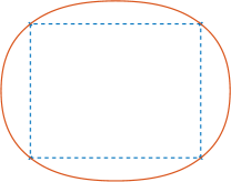
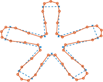
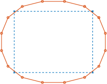
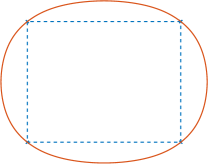
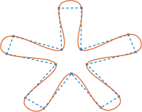
The basic limit function related to this mask is shown in Figure 3, and two examples of interpolating curves can be found in Figure 4. We have that and, via joint spectral radius techniques, one can prove that . By construction the corresponding subdivision scheme reproduces polynomials of degree . With respect to the primal interpolating quaternary scheme proposed by Conti et al. MR2775138 , which has a basic limit function supported in and reproduces quadratic polynomials only, the mask obtained here is much wider but achieve desirable properties in application such as -smoothness and reproduction of higher degree polynomials. On the other hand the primal interpolating quaternary -point scheme (see e.g. MR3702925 ) reproduces quintic polynomials as well but it has a basic limit function supported in .
Acknowledgements.
The authors are members of INdAM - GNCS, which partially supported this work.References
- (1) Alfred S. Cavaretta, Wolfgang Dahmen, and Charles A. Micchelli. Stationary subdivision. Mem. Amer. Math. Soc., 93(453), 1991.
- (2) Maria Charina and Thomas Mejstrik. Multiple multivariate subdivision schemes: matrix and operator approaches. J. Comput. Appl. Math., 349:279–291, 2019.
- (3) Sung Woo Choi, Byung-Gook Lee, Yeon Ju Lee, and Jungho Yoon. Stationary subdivision schemes reproducing polynomials. Comput. Aided Geom. Design, 23(4):351 – 360, 2006.
- (4) Charles Chui and Johan M. de Villiers. Wavelet Subdivision Methods: GEMS for Rendering Curves and Surfaces. CRC Press Boca Raton, FL, 2010.
- (5) Costanza Conti and Kai Hormann. Polynomial reproduction for univariate subdivision schemes of any arity. J. Approx. Theory, 163(4):413–437, 2011.
- (6) Costanza Conti and Lucia Romani. Dual univariate -ary subdivision schemes of de Rham-type. J. Math. Anal. Appl., 407(2):443–456, 2013.
- (7) Johan de Villiers and Mpfareleni Rejoyce Gavhi. Local interpolation with optimal polynomial exactness in refinement spaces. Math. Comp., 85(298):759–782, 2016.
- (8) Johan M. de Villiers, Charles A. Micchelli, and Thomas Sauer. Building refinable functions from their values at integers. Calcolo, 37(3):139–158, 2000.
- (9) Gilles Deslauriers and Serge Dubuc. Symmetric iterative interpolation processes. Constr. Approx., 5(1):49–68, 1989.
- (10) Serge Dubuc. Interpolation through an iterative scheme. J. Math. Anal. Appl., 114(1):185 – 204, 1986.
- (11) Serge Dubuc. de Rham transforms for subdivision schemes. J. Approx. Theory, 163(8):966 – 987, 2011.
- (12) Nira Dyn. Subdivision schemes in computer-aided geometric design. In Advances in Numerical Analysis, Vol. II (Lancaster, 1990), Oxford Sci. Publ., pages 36–104. Oxford Univ. Press, New York, 1992.
- (13) Nira Dyn. Interpolatory subdivision schemes. In Floater M.S. Iske A., Quak E., editor, Tutorials on Multiresolution in Geometric Modelling, pages 25–50. Springer, Berlin, Heidelberg, 2002.
- (14) Nira Dyn, Kai Hormann, Malcolm A. Sabin, and Zuowei Shen. Polynomial reproduction by symmetric subdivision schemes. J. Approx. Theory, 155(1):28–42, 2008.
- (15) Nira Dyn and David Levin. Subdivision schemes in geometric modelling. Acta Numer., 11:73–144, 2002.
- (16) Mpfareleni Rejoyce Gavhi-Molefe and Johan de Villiers. On interpolatory subdivision symbol formulation and parameter convergence intervals. J. Comput. Appl. Math., 349:354 – 365, 2019.
- (17) Graziano Gentili and Daniele C. Struppa. Minimal degree solutions of polynomial equations. Kybernetika, 23(1):44–53, 1987.
- (18) Nicola Guglielmi and Vladimir Protasov. Exact computation of joint spectral characteristics of linear operators. Found. Comput. Math., 13(1):37–97, 2013.
- (19) Thomas Mejstrik. Algorithm xxx: Improved invariant polytope algorithm and applications. arXiv:1812.03080v3, 2020.
- (20) Charles A. Micchelli. Interpolatory subdivision schemes and wavelets. J. Approx. Theory, 86:41–71, 1996.
- (21) Georg Muntingh. Symbols and exact regularity of symmetric pseudo-splines of any arity. BIT, 57(3):867–900, 2017.
- (22) Lucia Romani. Interpolating m-refinable functions with compact support: The second generation class. Appl. Math. Comput., 361:735–746, 2019.
- (23) Lucia Romani and Alberto Viscardi. Dual univariate interpolatory subdivision of every arity: Algebraic characterization and construction. J. Math. Anal. Appl., 484(1):123713, 2020.