A Machine Learning-based Approach to Detect Threats in Bio-Cyber DNA Storage Systems

Abstract

Data storage is one of the main computing issues of this century. Not only storage devices are converging to strict physical limits, but also the amount of data generated by users is growing at an unbelievable rate. To face these challenges, data centres grew constantly over the past decades. However, this growth comes with a price, particularly from the environmental point of view. Among various promising media, DNA is one of the most fascinating candidate. In our previous work, we have proposed an automated archival architecture which uses bioengineered bacteria to store and retrieve data, previously encoded into DNA. This storage technique is one example of how biological media can deliver power-efficient storing solutions. The similarities between these biological media and classical ones can also be a drawback, as malicious parties might replicate traditional attacks on the former archival system, using biological instruments and techniques.

In this paper, first we analyse the main characteristics of our storage system and the different types of attacks that could be executed on it. Then, aiming at identifying on-going attacks, we propose and evaluate detection techniques, which rely on traditional metrics and machine learning algorithms. We identify and adapt two suitable metrics for this purpose, namely generalized entropy and information distance. Moreover, our trained models achieve an AUROC over 0.99 and AUPRC over 0.91.

I Introduction

The World Wide Web [1] has transformed the way human beings create and share information, breaking down cultural barriers. Emerging communication technologies (e.g., 5G and Internet of Things) enabled seamless connectivity and novel applications. For example, social networks allow people to share their experience through messages, pictures, audio, and video recordings. As a consequence, we face an increasingly amount of data, bound to further grow as more and more devices will connect to the Internet in the future. Currently all these generated data are stored in large data centres, resulting in large investments in cloud services and infrastructures [2].

While these infrastructures are necessary and inevitable, they also bring along some challenges. Data centres consume phenomenal amounts of energy and heavily impact the environment [3] [4]. Besides, the energy required for powering and cooling the data centres place immense strain on the operation costs. Driven by these challenges, researchers have been exploring alternative storage mediums.

An emerging and promising approach is to store data into Deoxyribonucleic Acid (DNA). From a computing perspective, DNA represents biological cells’ software and determines organisms’ functionalities. This software enables different types of cells to operate as a collective system, such as tissues and organs. This key characteristic allows us to use cells as data storage units, where information is encoded into nucleotides and inserted in the DNA. There have been many proposed techniques for encoding information into genetic sequences. For example, Goldman et al. [5] developed a simple 2-bit encoding scheme, capable of storing a large quantity of data into DNA strands. A major question is the future practicality of DNA storage, and how we could integrate it in conventional data centres. Since we are dealing with biological substrates, we have to be aware of attacks that use either organisms or chemicals. The complication increases with biological systems equipped with random access functionalities. An example for random access was proposed by researchers from University of Washington and Microsoft [6]. In their work, the authors proposed multiple pools of DNA storage, where each DNA strand corresponds to binary data. To support random access capabilities, every strand has a primer (i.e., a specific sequence of nucleotides used as a starting point for DNA synthesis). Tavella et al. [7] proposed to store information within bioengineered bacteria [8] [9] [10], and retrieve it through a bacterial nanonetwork. Bacterial nanonetworks are artificial networks that exhibit molecular communication characteristics, and enable multi-hop links between motile and non-motile bacteria.

In this paper, we focus on the security implications of Tavella et al. [7] approach, where digital information is encoded into DNA plasmids, which are physically stored inside bacteria. In particular, bacteria are known to interact and communicate as part of their social ecosystem, both intraspecies and interspecies. Communication is critical for bacteria to survive collectively as a population and evolve through different environmental changes. When information is stored in bacteria, population interference can occur from other bacteria living within the same environment. Such interference need to be monitored in order to ensure that the retrieval process maintains an acceptable level of reliability. Giaretta el al.  [11] presented how security can affect bacterial nanonetworks, by blocking or deviating the movement of motile bacteria towards an intended location.

In Figure 1, we present an architecture where bacterial nanonetworks can be integrated into conventional data centres. The bacterial storage can be located in data centres, or can be part of a remote device owned by the end user, such as an Internet of Things (IoT) device. Research showed that current IoT devices are susceptible to security attacks [12], making them unfit candidates for holding complex entities like bacterial networks. Moreover, IoT devices generally lack in computational power, increasing the challenge in deploying monitoring algorithms to detect security attacks. Data centres are better candidates for integrating a biological infrastructure. First, they exhibit isolation which allows them to safely host a DNA storage system based on bacterial nanonetworks. Second, they have access to enough computational power for storing and running monitoring algorithms.

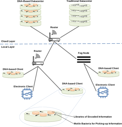
Figure 1: Architecture of a mixed network, where traditional electronic devices and servers co-exist with DNA-based devices.

In our study, we investigate two types of algorithm for detecting attacks on the bacterial nanonetwork DNA storage. We use information metrics, previously used for detecting Distributed Denial of Service (DDoS) attacks in conventional networks [13], and we use Machine Learning (ML) techniques.

The contributions of this paper are manifold:

1. An analysis of bacterial nanonetwork DNA storage system from a computer science perspective, highlighting similarities and differences with conventional storages;

2. A security attack that uses competing bacteria to disrupt the bacterial nanonetwork infrastructure;

3. Information metric techniques reformuled for detecting DDoS attacks in conventional networks, together with an assessment of such techniques for bacterial nanonetwork storages;

4. Machine learning algorithms for monitoring bacterial nanonetworks and detecting attacks;

5. A thorough evaluation of all the presented techniques through extensive simulations.

We organize this paper as follows: Section II describes the DNA automated archive and the different attacks that a malicious user could execute into it. Section III describes traditional metrics for detecting DDoS attacks and how we can adapt them to our scenario. Section IV explains how machine learning can be used for the same purpose. In Section V we assess the attacks dangerousness, as well as the effectiveness of our detection techniques. Last, in Section VI we discuss our results and draw our conclusions.

II System model

In this section, we describe the functioning of bacteria-based DNA-based storage devices and the corresponding attacks that can be lead onto these systems.

II-A DNA storage

The DNA automated archive [7] is a biological storage system that combines two different components: DNA encoding and bioengineered bacteria. The first component provides a way for transferring and translating digital information into DNA, while the bacteria are used as data storage and access mechanism. Figure 2 describes the overall system architecture of the system proposed in [7]. Digital information is firstly encoded into nucleotides, and for this the authors use different encoding techniques. The synthesized genes of the encoded nucleotides are inserted into plasmids, and plasmids are inserted into bacteria through the transformation process. To ensure motility restriction, these bacteria are place on solid agar (i.e., a jelly-like substance used to measure microorganisms’ ability to move). The motility-restricted bacteria with different data are placed into specific regions of the grid, as illustrated in Figure 2. In the event that a read operation needs to be performed, motile bacteria are released from A, swim towards the compartment, and then conjugate with the motile-restricted bacteria to retrieve the plasmids with the encoded information. Once this is complete, bacteria swim towards position C to deliver the plasmids. Conjugation is a process where bacteria come together and form a physical connection that allows them to transfer plasmids between each other, and this process has a probability associated with it. At position C, the plasmids are retrieved, sequenced to obtain the data, and decoded back into digital format.

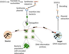
Figure 2: Overall system architecture of the DNA archival system that enables reading using bacterial nanonetworks. Motile bacteria (in grey) swim from the source towards each of the library points, which contain different information. Reached the motile-restricted bacteria, conjugation starts to retrieve the encoded information contained into the plasmid. Last step, motile bacteria swim towards the Target, where the plasmid is retrieved through sequencing processes.

A key requirement for the motile bacteria is the capability of swimming towards an accurate point. This allows to conjugate with the correct batch of motile-restricted bacteria, and retrieve the right plasmid with the encoded information. This is where the proposed Molecular Positioning System (MPS) [7] plays a role. As suggested by Okaie et al. [10], it is possible to deploy chemoattractants and redirect engineered-bacteria by means of chemotaxis (i.e., movement as a response to chemical stimuli). This pairs well with MPS [7], which is based on the receptor saturation addressing technique, proposed by Moore and Nakano [8] [9].

II-B Vulnerabilities

Regardless of the fact that it is based on bacterial nanonetworks, the DNA archive [7] is, to many extents, similar to electronic storage systems. Therefore, it is prone to most of the common databases attacks. Here, we propose two examples of these attacks: Denial of Service (DoS) and sniffing.

II-B1 Denial of Service

In order to share DNA, bacteria use a method called conjugation. During this process, two bacteria physically connect to each other to share plasmids (i.e., circular DNA strands). However, each bacterium can conjugate only with one bacterium. Thus, if attackers spread their own bacteria around the clusters area, the bacteria conjugate with the set of bacteria that contain the encoded data, as Figure 3 illustrates. Malicious bacteria move from point $C$ to the cluster, cluttering the system, and after completing the conjugation process reach point $D$. In this way, the legitimate bacteria that are meant to retrieve the DNA are not able to conjugate and access the information in the archive. This equals to a DoS attack on a database, since it prevents the main feature of the archive, retrieving stored data. Besides blocking and cluttering the clusters of motile bacteria, the cluttering can also occur at the destination where the bacteria are collected before they are pulled into the sequencer.

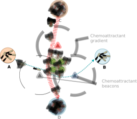
Figure 3: Example of DoS scenario. Legitimate bacteria move from starting point A to the agars containing the storage bacteria. Once the conjugation is complete, they move towards their destination B. Malicious bacteria move from C to D trying to conjugate with the ones in the agar, blocking the retrival process of the legitimate bacteria.

II-B2 Sniffing

To extract data from the biological storage system, the bacteria need to pick-up the data contained in the clusters and to reach the machine that performs DNA sequencing. During the trip from the archives to the sequencer, an attacker could place a swarm of bacteria in the middle. This would cause the bacteria to conjugate with the ones carrying the encoded information. Consequently, the malicious user can obtain the encoded information without accessing the machine connected to the DNA sequencer. In a network scenario, it would be the equivalent of listening on a channel and sniffing packets.

III DoS information metrics

One way to evaluate an experiment is to define a metric, a standard for measuring a particular characteristic of the experiment. For example, in the field of cybersecurity it is important to measure the damage that an attack (e.g., a DoS) can produce to an infrastructure, or the robustness of the infrastructure in general. Each metric is strictly correlated to what it measures. Therefore, the same metric can perform differently based on the scenario in which it is applied.

It is possible for an attacker to elude detection metrics. For example, if we perform a DoS attack and we do not want to be tracked, we can use multiple machines to conduct the attack. By distributing the outgoing traffic over different IPs we make it harder for the victim to trace us, achieving a Distributed DoS (DDoS). Another way of eluding DoS detection metrics is to maintain a low-rate of traffic sent by the malicious computers, so that it negatively affects the service without exceeding the warning threshold.

Therefore, we need a tool that can overcome similar scenarios. Xiang et al. [13] developed an algorithm based on statistical methods to detect a low-rate DDoS attack and traceback the IP of the attacker. Given a Local Area Network (LAN) and a supervisor that monitors the network traffic, their algorithm is based on the following assumptions:

1. the supervisor has full control of all the routers;

2. they extracted an effective feature (e.g., IP addresses) of network traffic to sample its probability;

3. the supervisor obtained and stored the average traffic of the normal, as well as the local thresholds $\sigma_{f_{i}}$ and $\sigma_{f(R_{i})}$ on its own routers in advance;

4. on all routers, the traffic follows Poisson distribution and the normal traffic follows a Gaussian noise distribution. As stated by Xiang et al. [13], it is widely accepted that the Poisson distribution function can simulate the DDoS attack traffic in aggregation and the fractional Gaussian noise function can be simulate real network traffic in aggregation.

The authors redefine two metrics commonly used in information theory: generalized entropy and information distance. Generalized entropy is a measure of uncertainty associated with a random variable. The more random the information, the bigger the entropy; viceversa, the greater the certainty related to the information, the smaller the entropy. Given a set of events $\{x_{1},x_{2},x_{3},\ldots,x_{n}\}$, their associated probabilities ${p_{1},p_{2},p_{3},\ldots,p_{n}}$ and the following property:

$$0\leq p_{i}\leq\leavevmode\nobreak\ \forall i=1\ldots n,\ \sum_{i=1}^{n}p_{i}=1,$$ (1)

the generalized entropy is defined as follows:

$$H_{\alpha}(x)=\frac{1}{1-\alpha}log_{2}\left(\sum_{i=1}^{n}p_{i}^{\alpha}\right),\alpha\neq 0,$$ (2)

where $\alpha$ is the order of the entropy. When $\alpha\rightarrow 1$, the formula converges to the Shannon entropy:

$$H_{1}(x)=-\sum_{i=1}^{n}p_{i}log_{2}p_{i}.$$ (3)

One of the most important properties of the generalized entropy is that, given $\alpha>1$, it increases the deviation between the different probability distributions, compared to the Shannon entropy [14] [15]. A high probability event contributes more to the final entropy than to the Shannon entropy when $\alpha>1$, and a low probability event contributes more when $\alpha<1$. Consequently, we can obtain different entropy values based on the different values of $\alpha$.

Finally, the information distance measures the divergence between two probability distributions. Let $P=(p_{1},p_{2},\ldots,p_{n})$ and $Q=(q_{1},q_{2},\ldots,q_{n})$ be two discrete complete probability distribution with the same properties described in Equation 1. The information distance can be calculated as:

$$D_{\alpha}(P||Q)=\frac{1}{\alpha-1}log_{2}\left(\sum_{i=1}^{n}p_{i}^{\alpha}q_{i}^{1-\alpha}\right),\alpha\geq 0.$$ (4)

Note that $D_{\alpha}(P||Q)\neq D_{\alpha}(Q||P)$. In other terms, the information distance is not symmetric. Based on the value of $\alpha$, one of the two distributions (i.e., the one to the power $(1-\alpha)$) may not be able to contain events where the associated probability is equal to 0. The authors define such distribution as continuous. For $\alpha\rightarrow 1$, the information distance becomes the Kullback-Leibler divergence:

$$D_{1}(P||Q)=\sum_{i=1}^{n}p_{i}log_{2}\left(\frac{p_{i}}{q_{i}}\right).$$ (5)

In [13], Xiang and colleagues modified the information distance equation to satisfy a few properties (namely, additivity, asymmetry and incresing function of $\alpha$) in order to make it compliant to the formal definition of metric. The final result is given in Equation 6:

$$D_{\alpha}(P,Q)=D_{\alpha}(P||Q)+D_{\alpha}(Q||P)=\\ \frac{1}{\alpha-1}log_{2}\left(\sum_{i=1}^{n}p_{i}^{\alpha}q_{i}^{1-\alpha}\cdot\sum_{i=1}^{n}q_{i}^{\alpha}p_{i}^{1-\alpha}\right).$$ (6)

In this case, none of the two probability distributions can contain events with an associated probability equals to zero. In the end, Xiang et al. used the information distance metric to develop a collaborative DDoS attack detection algorithm, which can be found in [13].

III-A Metrics as detection mean

Generalized entropy and information distance are based on probability distributions of values, while in our case we have a distribution of value over time. However, a distribution over time can be converted to an approximation of a probability distribution. In fact, given the initial number of bacteria $N_{i}$ and the total simulation time $T$, we can calculate the probability of observing a certain number of bacteria $b$ as:

$$P(x=b)=\frac{\sum_{t=0}^{T}B(t)=b}{N_{i}},$$ (7)

where $B(t)$ is the number of bacteria counted at time $t$ and:

$$(B(t)=b)=\begin{cases}1&\mbox{if there are {b} bacteria at time t,}\\ 0&\mbox{otherwise.}\end{cases}$$ (8)

The main idea is to use the two metrics to detect if an attack on our archive is taking place. Intuitively, the traffic (i.e., the number of bacteria and how they are distributed over time) is different whether the system is functioning normally or it is under attack. As a result, we define the Algorithm 1 to convert the time sequence into a (sample of) probability distribution. The reason behind this pre-processing is that we wait for bacteria to swim towards their destination, which can take a long time. By defining a long period of time $T$, we can assume a stable mean of bacteria that reach their destination. In this way, we can use the generalized entropy and information distance in our scenario.

Input: $N_{i}$ number of bacteria, $D$ array of distribution over time.

Output: $P$ array of probabilities.

$v\leftarrow 0$;

while $v\leq N_{i}$ do

       $P(v)\leftarrow countValueInArray(v,D)$;

       $v\leftarrow v+1$;

      

end while

$P\leftarrow divideElementWise(P,length(D))$;

Algorithm 1 Converting a time series to an approximation of a probability distribution.

As long as the sum of these probabilities is not zero, we can calculate the entropy and measure its changes due to an intrusion in the archive. Based on the definition, generalized entropy gives more relevance to rare events: the less likely an event, the bigger the entropy. This implies that when we have a really low number (e.g., 10) of outgoing “packets” (i.e., bacteria reaching the destination area) and we lose one of them, the event becomes very frequent ($1/10=10\%$) and the generalized entropy is less relevant compared to a scenario where we have a loss of 1 packet over 150 ($1/150=0.\overline{66}\%$).

Nevertheless, we need to make some changes in order to use the generalized distance. One of the main assumption made by Xiang et al. [13] is that the probability distributions involved in the calculation must be continuous. This is not our case, because it is very likely that two different data extractions lead to two different time series of bacteria, due to the randomness in bacteria movement. As a result, it may happens that a certain value never appears in one series, while it does in other series.

There are two possible way of adapting the metric to our case: using dummy values and transforming the distributions to make them continuous. The usage of dummy values implies substituting each 0 that make the distribution non-continuous with a fixed value (e.g., $10^{-3}$). However, the insertion of a low number would change significantly the value of the metric; on the contrary, a high number would invalidate the fact that the sum of all probabilities is equal to 1. Thus, truncating the distributions in order to make them continuous is a better option. Let us suppose that our distribution is composed of 4 values and their associated probabilities $\{(v_{0},p_{0}),(v_{1},p_{1}),(v_{2},p_{2}),(v_{3},p_{3})\}$. While it is true that the removal of an event from the distribution (e.g., $(v_{3},p_{3})$) implies a loss of information, such a loss would not be so impactful. Indeed, the information that a specific event contains is also partially contained in other events: for example, we know that $p_{3}=1-\sum_{i=0}^{2}p_{i}$. Algorithm 2 describes how, given two probability distributions, we can make them continuous according to Xiang et al.’s [13] definition.

Input: $P$ and $Q$, arrays of probabilities.

Output: $Pc$ and $Qc$, arrays of continuous probabilities.

$Pc,Qc\leftarrow emptyArray()$;

$len\leftarrow min(length(P),length(Q))$;

$i\leftarrow 0$;

while $i<len$ do

       if $P(i)\neq 0$ and $Q(i)\neq 0$ then

             $Pc\leftarrow append(Pc,P(i))$;

             $Qc\leftarrow append(Qc,Q(i))$;

            

       end if

      $i\leftarrow i+1$;

      

end while

Algorithm 2 Converting two probability distributions into two continuous probability distributions.

In this way, we can use the distance metric to measure the divergence by comparing two different scenarios. This implies that the distance metric is a better way of measuring the diversity of two events, because it compares them directly, while the generalized entropy compares their respective values.

IV Machine learning for detection

Despite the appropriateness of a metric, in most cases its mathematical development requires time and resources from researchers. An automated approach would be better in terms of efficiency and efficacy, given that it could extract abnormalities from the data and automatically adapt to new scenarios.

In the cybersecurity field, one of the main tools recently used for detection algorithms is machine learning (ML) [16] [17]. For example, ML is used for intrusion detection [18], as well for DoS [19] and DDoS detection [20] [21]. By using a learning approach, we do not need to develop a different metric for each kind of attack. Instead, we can give a lot of examples (i.e., behaviour of the system under normal circumstances and under attack) to a machine learning algorithm, allowing it to learn to distinguish different scenarios. Moreover, if the algorithm has been trained enough, we could potentially reuse it for different kind of attacks.

Machine learning is usually divided in two main categories: supervised and unsupervised learning. In supervised learning, we have a set composed of examples tuples $\{(x_{0},y_{0}),(x_{1},y_{1}),\cdots(x_{n},y_{n})\}$ where $x_{i}$ is the feature of the example, and $y_{i}$ is its label (i.e., an assigned category). Usually, the task of a supervised learning algorithm is to minimize the error related to a function that involves these examples, in order to be able to predict categories (classification) or values (regression). On the other hand, unsupervised learning does not require any category, and the categorization is based upon similarities among the features. Ideally, unsupervised learning algorithms learn to categorize the example without any external support. However, in some cases it is really hard to distinguish similar examples without any indications, because features can be really similar even when they indicate different classes. Moreover, given the pace of virtual simulations, we can generate samples to train the algorithm without the necessity of observing a real system being attacked.

In our case, we can obtain two different information from our simulations: the distribution of bacteria over time, and the probability of observing a specific amount of bacteria over the whole simulation. In addition, we also know the number of bacteria used to retrieve the data and the number of malicious bacteria. Consequently, we define three different types of features that we will feed to our algorithm: (i) the number of bacteria that were able to reach their destination in an interval between two sampling periods, (ii) the cumulative number of bacteria that reached their destination up to a specific moment, and (iii) a sample of probability distribution, as described in Section III-A. From now on, we will refer to these features with the names of “count”, “sum” and “sample”. Using this data, our goal is to train a machine learning algorithms (e.g., Logistic Regression, Support Vector Machine, or Neural Networks) capable of distinguishing benevolent and malicious traffic in our system during a DoS attack.

In the following sections, we walk through the steps for pre-processing the data, selecting and evaluating the model, and predicting the results.

IV-A Pre-processing

One of the most important ML phases is data pre-processing. Usually, it is composed of four steps: (a) cleaning:detecting, removing, and correcting corrupt data; (b) integration:merging in a proper way different kind of data, in order to obtain a unique data set; (c) transformation:changing data values to meet some requirements (e.g., we want features with a specific average and standard deviation), or removing noise; (d) reduction:removing from the data set entries that are useless/redundant.

In our case, we do not need to go through the integration, but we need to address the other three points. Given the different numbers of legitimate bacteria for the simulations, we obtain different probability distributions from Algorithm 1. For a scenario that has a lower number of bacteria than other cases, we do not calculate the probability for the same range of values. For example, if a scenario has $n_{1}^{max}=50$ bacteria and the other scenario has $n_{2}^{max}=100$, the probability distribution for the first one does not include the probabilities for values greater than 50. Consequently, we need to fill in the missing probability values with zeros. In addition, we normalize all the features so that they follow a normal distribution $N(0,1)$. As we described in Algorithm 2, we also remove all the columns that contain zero in all the entries, both from the left and the right side of the data set, in the same way trimming a string would remove the whitespaces at the beginning and at the end of it.

IV-B Model selection

Different predictors have different characteristics. Some of them produce poor results if they are fed with small data sets, while others can perform good even with small data sets. Other models are suited for binary classification (i.e., two possible outcomes), while others can distinguish among more classes. Therefore, we need to choose the best predictor for our specific task.

Our main goal is to detect whether our system is under attack or not. Consequently, we have to perform a binary classification where 0 indicates under attack and 1 stands for normal traffic. We test five different classifiers: Support Vector Machine, Multi-layer Perceptron, Random Forest, K-Nearest Neighbors, and Logistic Regression.

IV-C Metrics

As we previously mentioned, in order to measure the quality of our choices and results, we need to define some metrics. There are some metrics widely used in machine learning which consider the capability of the predictor to produce correct results. In binary classification, given an example $(x_{i},y_{i})$ and its predicted value $y^{\prime}_{i}$, there are four possible scenarios: (i) True Positive (TP), where $y_{i}=y^{\prime}_{i}=1$; (ii) True Negative (TN), $y_{i}=y^{\prime}_{i}=0$; (iii) False Positive (FP), $y_{i}=0$ and $y^{\prime}_{i}=1$; (iv) False Negative (FN), $y_{i}=1$ and $y^{\prime}_{i}=0$.

From these four possible outcomes, we can define the following metrics:

• Accuracy ($\alpha$): $\frac{TP+TN}{TP+FP+TN+FN}$;

• Precision ($\pi$): $\frac{TP}{TP+FP}$;

• Recall ($\rho$, also called Sensitivity or True Positive Rate): $\frac{TP}{TP+FN}$;

• F1 score: $2\frac{\pi\rho}{\pi+\rho}$;

• Specificity (or True Negative Rate): $\frac{TN}{TN+FP}$;

• False Positive rate: $1-Specificity$;

• AUC (Area Under Curve): the area under a curve that represents the ratio between correct and wrong predictions (e.g., precision-recall curve).

Accuracy is a general score describing how many guesses from the predictor are correct, but it is not reliable in case of unbalanced data sets. Sensitivity (i.e., recall) and specificity indicate, respectively, the proportion of positives and negatives that are correctly identified as such. Precision represents the number of actual positives, among all the predicted positives. The F1 score is a combination of precision and recall, which also describe the accuracy of the predictor in case of an unbalanced dataset. Finally, the Receiver Operating Characteristic (ROC) curve plots True Positive Rate (TPR) versus False Positive Rate (FPR) at different discrimination thresholds - i.e., a value used to determine whether to classify a sample as one class or another. Thus, the ROC curve represents the TPR as a function of the FPR. Similarly, the Precision-Recall curve plots precision versus recall while varying the discrimination threshold - this particular curve is ideal for unbalanced datasets. By calculatitng the Area Under Curve (AUC) for these two different measures, we obtain an aggregate measure of performance across all possible classification thresholds. We define the AUC for ROC as AUROC and the AUC for Precision-Recall curve as AUPRC.

IV-D Training and parameter tuning

Usually, before training a machine learning algorithm we must divide the data set in three different subsets:

• training set: the part of the data used to train the algorithm;

• validation set: the subset used to choose the model, and tune its hyperparameters;

• test set: the data used to evaluate the efficacy of the algorithm, after it has been trained.

In this way, we evaluate the algorithm with neutral data that was not part of its training. Moreover, the division of training and test set reduce the risk of overfitting, which is the phenomenon of producing an analysing that corresponds too closely to a specific data set. One further step for avoiding overfitting is to use cross validation. In particular, k-fold cross validation is a technique that splits the data into $K$ chunks of the same size, trains the model with $K-1$ chunks, and uses the remaining data as validation set. These steps are then repeated for each chunk. Cross validation helps both with overfitting and parameter tuning, increasing the flexibility of an evaluation.

In our case, we split our data sets using the 70% of it as training (and validation) set, and the remaining 30% as test set. We implement this division using the train_test_split function from Scikit-learn machine learning library [22]. In addition, we use the GridSearchCV class to execute an exhaustive parameters search using cross validation. Table I lists all the parameters that we investigate using the cross validation method.

TABLE I: Parameters inspected during cross validation. The parameters name follows the nomenclature used by Scikit-learn [22]

Model	Parameters
MLP	hidden_layer_sizes, solver, learning_rate
KNN	n_neighbors, weights, algorithm
SVM	C, gamma, kernel, max_iter
RF	n_estimators, max_features
LR	fit_intercept

V Evaluations and Results

We defined different tools (i.e., metrics and machine learning algorithms) to detect if a malicious user is trying to compromise a DNA-based archive. In this section, to assess the quality of such tools, we run a number of simulations that replicate the scenarios illustrated in Section II-B. Each simulation represents one possible attack, demonstrating how this vulnerability can affect the storage system. In the end, we implement the different detection techniques described in Section III and Section IV to verify their efficacy.

For each of the following simulations, the maximum amount of bacteria contained in each cluster is 50, as mentioned by Tavella et al. [7]. We conform to this parameter in order to enable comparison between the data obtained during an undisturbed run of the system and the following simulations. If the bacteria are not able to retrieve the whole file within 120 virtual minutes (i.e., two hours in the simulation), we stop the simulation. Finally, we indicate the intervals as tuples $[l,u,s]$ where $l$ is the lower bound, $u$ is the upper bound (both included in the interval), and $s$ is the step size. For example, the tuple $[10,30,10]$ indicates a range composed of the values $10$, $20$, and $30$.

V-A Attacks simulations

In this section, we describe the simulations we conducted for evaluating the disruption of a DoS attack. In addition, we define the dangerousness of an attack in terms of delay and information loss, which is the incapability of retrieving data within a fixed amount of time.

We have previously illustrated in Figure 3 how, during a Denial of Service attack, malicious bacteria move towards the clusters and conjugate with the bacteria containing the encoded data, obstructing the legitimate bacteria. In our simulations, we decided to vary the number of legitimate bacteria in the range $[10,150,10]$, according to the simulations conducted in [7], and the number of malicious bacteria in the range $[0,1900,100]$. Until the amount of legitimate and malicious bacteria is lower than the total amount of bacteria in the cluster, it is not possible to detect any kind of attack because the cluster is not running at maximum conjugation rate. However, since the conjugation has a probability approximated by a Normal distribution with mean 0 and standard deviation 1, it is not certain that we are able to detect any difference even if the sum of the two types of bacteria is slightly greater than the threshold.

Figure 4 shows how the percentage of retrieved file changes with respect to the number of legitimate and malicious bacteria. Even with a really high amount of attackers, it is sufficient to use 150 retrievers to extract the whole file from the archive. This shows that the percentage of retrieved file is not a good measure to detect an attack. Figure 5 illustrates how the time to retrieve the file is affected by the number of bacteria. In this case, we can see how the number of attackers affects the final time, increasing it from  40 minutes (150 retrievers vs. 0 attackers) to  100 minutes (150 retrievers vs. 1900 attackers). In many cases, such as with attackers $>1000$ and retrievers $<100$, the average time to retrieve the file gets really close to the 120 minutes threshold.

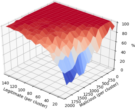
Figure 4: Correlation among the number of engineered motile bacteria, number of attackers and percentage of file retrieved. If the percentage is lower than 100%, it means that the engineered motile bacteria were not able to retrieve the whole file in less than 120 minutes.

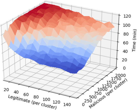
Figure 5: Correlation among the number of engineered motile bacteria, number of attackers and time necessary to retrieve the whole file. If the time is greater or equal to 120 minutes, then the engineered motile bacteria were not able to retrieve all the information.

In Section II-B2, we hypothesised that a malicious user could steal a copy of the archived information, without being noticed. From the results in Figure 4 and Figure 5, we can deduce that an attacker could introduce a small number of bacteria and obtain the archived data, while keeping the delay low enough to avoid being detected.

V-B Evaluation of information metrics

Before analysing the importance of the metric order $\alpha$, let us recall its role. Given a metric, such as the generalized entropy, its order $\alpha$ increases/reduce the importance of an event. Let $p$ be the probability of an event, with $0\leq p\leq 1$. If $p\neq 1$, there are two different scenarios:

1. if $\alpha>1$, then $p>p^{\alpha}$;

2. otherwise ($\alpha<1$), $p<p^{\alpha}$.

Consequently, whenever we impose the metric order below 1, we increase the value corresponding to the probability of an event. With really small values of $\alpha$, the closer the probability is to 0, the bigger is the amplification. For example with $\alpha=0.1$ and $p=0.1$, $0.1^{0.1}-0.1\approx 0.69$, while with $\alpha=0.1$ and $p=0.5$, $0.5^{0.1}-0.5\approx 0.43$. In light of this, if we use an order which is too small, we risk to flatten the diversity between probabilities.

Here we present the most significant results; for the detailed results, we refer the reader to Appendix A. We test four different orders: $0.5,2,5,10$. We notice that there is no significant difference in using $\alpha=2$, $\alpha=5$ or $\alpha=10$, so we decide to remove 5 and 10 (i.e., the values that could cause unwanted spikes in our curves)from the possible orders for the entropy. Figure 6 shows how the metric changes with different numbers of legitimate and malicious bacteria, for $\alpha=2$.

Through our experiments we also found out that $\alpha$ severely affects the information distance. When the order is below 1, it drastically flattens the differences. When the order is too high (e.g., 10) the information distance lacks of monotonous behaviour, presenting a lot of spikes over the curve. As a consequence, we discard 0.5 and 10 as values for the information distance. Figure 7 illustrates the behaviour of the metric with order $\alpha=2$.

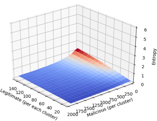
Figure 6: Generalized entropy as a function of benevolent and malicious bacteria. The sampling period is equal to 10 seconds and $\alpha=2$.

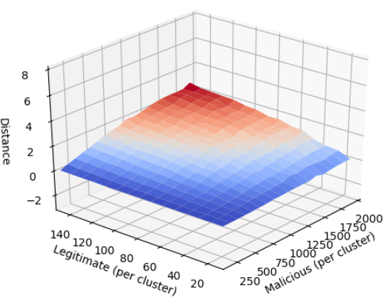
Figure 7: Information distance as a function of benevolent and malicious bacteria. The sampling period is equal to 10 seconds and $\alpha=2$.

To summarize, we have two order values for the entropy ($0.5$ and $2$) and for the information distance ($2$ and $5$) which present different values for the respective metrics based on whether the system is under attack or not.

Finally, our sampling frequency plays a major role in the values of our metrics: a low sampling frequency can hide the differences between distributions, while a high sampling frequency is hard to implement from a technical point of view, due to separation of bacteria and count. Therefore, we decide to explore different scenarios where we gradually decrease the sampling frequency. Given 6 different sampling periods - 10, 20, 30, 60, 120, and 240 seconds - we observe in Figure 6 no significant variations for the generalized entropy. On the other hand, the information distance is heavily affected by the sampling period, changing its behaviour from detecting changes in the number of malicious bacteria while using a small sampling period (Figure 7) to detecting changes in the number of legitimate ones while using a larger sampling period (Figure 8).

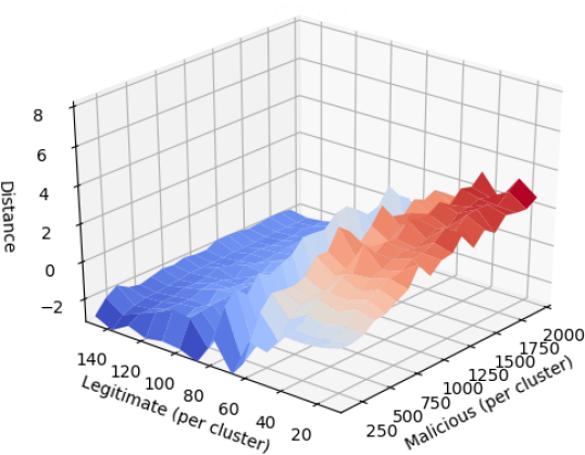
Figure 8: Impact of number of legitimate/malicious bacteria on information distance with $\alpha=2$ and sampling period of 240 seconds. Compared to Figure 7, the sampling period has a significant impact.

V-C Evaluation of Machine Learning

Here we describe in detail the results for binary classification. For each metric, we discuss which are the best features and models to use in order to obtain the best classificator.

Let us recall that the accuracy is defined as the ratio of correct predictions over the whole set of predictions, It gives us an idea about the efficacy of our predictor. However, if one class cardinality is much larger than the other, correct predictions over the majority class have a stronger influence over the accuracy. Thus, we need to consider metrics that separates correct predictions for positive and negative samples, such as sensitivity, specificity, and precision. Hence, we decide to use the AUROC and the Area Under Precision-Recall curve as a combination of the best metrics for our scenario.

Figure 9 shows how the correctness of our predictor is affected by the different features and different sampling periods, using the Area under the ROC curve and Precision-Recall curve. If we take into consideration only the AUROC (Figure 9a), we can observe that varying sampling periods does not drastically affect the score - i.e., low standard deviation. The “sum” feature appears to be the best for all the classifiers. Regarding the different classification algorithms, K-NN is the one with the poorest performance and the highest standard deviation. On the contrary, Random Forest is one of the best algorithms across all the classifiers, with a negligible variance. We can see that there is no feature that is capable of reducing the standard deviation for all the algorithms simultaneously and K-NN remains the algorithm that performs worse in most of the scenarios. Even if we consider a different score, the feature that brings most of the algorithms to the same level is “sum”. In fact, the importance of using this feature is remarked by Figures 19 to 21 in Appendix B.

Finally, given a sampling period of $T=10(s)$, Figures 16 to 18 and Figures 19 to 21 describe how every algorithm performs over different features, using ROC curves and Precision-Recall curves. In Figures 16 to 18 we notice that no algorithm, except for K-Nearest Neighbors, scores an Area Under ROC curve below 0.95. On the other hand, all the algorithms score above 0.98 with the “sum” feature.

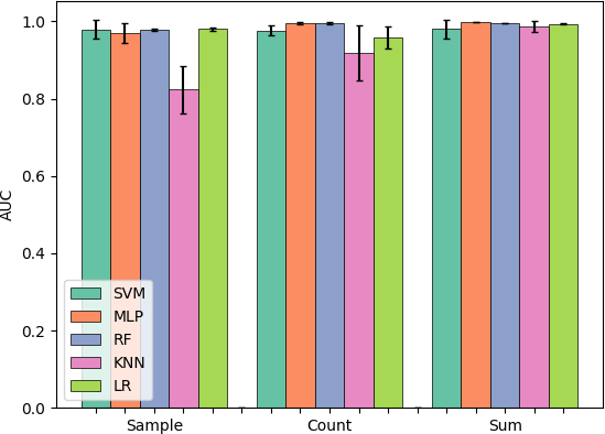
(a) Area Under ROC curve.

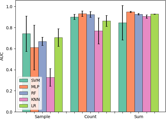
(b) Area Under Precision-Recall curve.

Figure 9: Mean and standard deviation of the Area Under ROC curve and Precision-Recall curve for different algorithms, calculated using a sampling period of 10, 20, 30, 60, 120 and 240 seconds.

VI Conclusion

Technology incredibly evolved and revolutionized society over the last decade. Sometimes technological breakthroughs trigger the necessity for an update of existing tools. In the case of Big Data, one of the obvious consequences is the necessity for new storage devices, able to keep up with the data trend.

With its high capacity/volume ratio, DNA is among the most interesting candidates for solving the storage issue. However, biological devices storing information in their DNA can suffer of security issues ascribed to traditional electronic architectures. A malicious user can use malicious bacteria to replicate conventional attacks, such as DoS attacks, on a bacterial nanonetworks. In order to mitigate these risks, we need to deploy some countermeasures to prevent and detect these new kind of threats. In this paper, we focus on two different detection techniques: metrics and machine learning. In particular, we adapt to our scenario metrics for detecting traditional DoS attacks.

Applying some changes to the metrics defined by Xiang et al [13], we manage to distinguish legitimate traffic from malicious traffic. Moreover, we use machine learning algorithms to perform binary classification using three different features, in order to analyse the bacterial network traffic. Considering the “sum” feature, we scored an AUROC over 0.99, and an AUPRC over 0.91, proving that we can reliably distinguish whether the system is under attack or not. We also showed that - due to the nature of our data - K-NN is the worst performing classification algorithm, while RF proved to be most consistent, across different features.

Appendix A Metrics results

Figures 10 to 12 and Figures 13 to 15 show the results we obtained by varying the order $\alpha$ for generalized entropy and information distance. By increasing $\alpha$, the generalized entropy becomes less responsive to variations in the number of malicious bacteria. On the other hand, the information distance lacks of monotic behaviour, as we can see in by the spikes in Figure 14 and Figure 15.

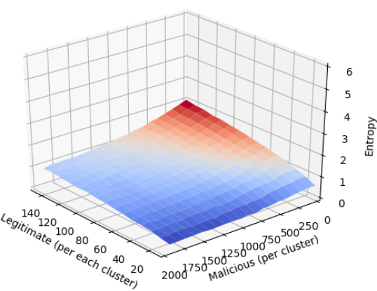
Figure 10: Impact of metric order on generalized entropy with sampling period $T=10s$ and $\alpha=0.5$.

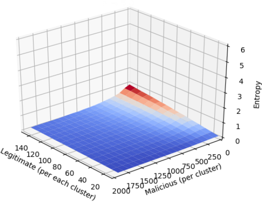
Figure 11: Impact of metric order on generalized entropy with sampling period $T=10s$ and $\alpha=5$.

Figure 12: Impact of metric order on generalized entropy with sampling period $T=10s$ and $\alpha=10$.

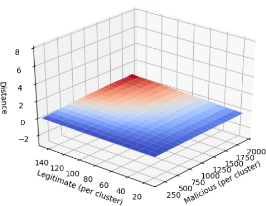
Figure 13: Impact of metric order on information distance with sampling period $T=10s$ and $\alpha=0.5$.

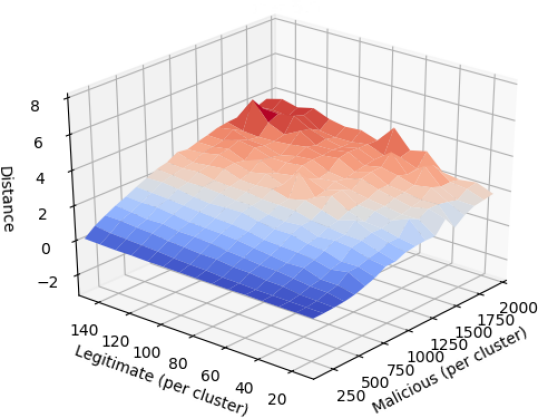
Figure 14: Impact of metric order on information distance with sampling period $T=10s$ and $\alpha=5$.

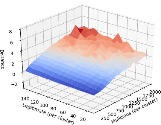
Figure 15: Impact of metric order on information distance with sampling period $T=10s$ and $\alpha=10$.

Appendix B Machine learning results

Figures 16 to 18 and Figures 19 to 21 illustrate the ROC and Precision-Recall curve for each model, using a sample period of 10 seconds. For each different model and feature, we present the respective score in the legend of the graphs. As previously discussed, we can see that the K-NN algorithm is the one performing worst over different features.

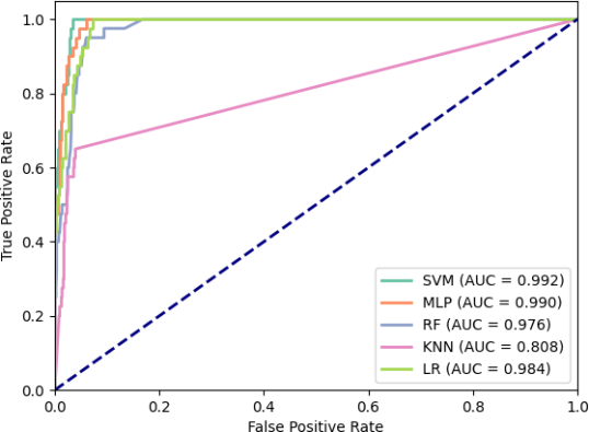
Figure 16: ROC curve of different algorithms using the sample feature and $T=10s$ as sampling period.

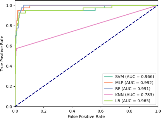
Figure 17: ROC curve of different algorithms using the count feature and $T=10s$ as sampling period.

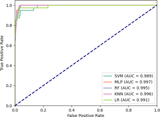
Figure 18: ROC curve of different algorithms using the sum feature and $T=10s$ as sampling period.

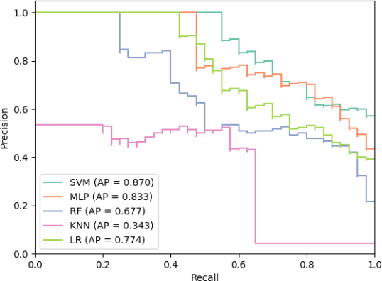
Figure 19: Precision-recall curve of different algorithms using the sample feature and $T=10s$ as sampling period.

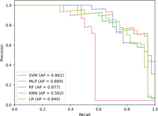
Figure 20: Precision-recall curve of different algorithms using the count feature and $T=10s$ as sampling period.

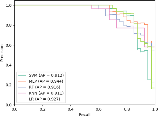
Figure 21: Precision-recall curve of different algorithms using the sum feature and $T=10s$ as sampling period.

References

- [1] “The original proposal of the www.” Accessed on 2018-06-22.
- [2] R. Miller, “Facebook builds exabyte data centers for cold storage,” 2013. Accessed on 2017-05-20.
- [3] B. Walsh, “Your data is dirty: The carbon price of cloud computing,” 2014. Accessed on 2018-06-11.
- [4] J. Glanz, “Power, pollution and the internet,” 2012. Accessed on 2018-06-11.
- [5] N. Goldman, P. Bertone, S. Chen, C. Dessimoz, E. M. LeProust, B. Sipos, and E. Birney, “Towards practical, high-capacity, low-maintenance information storage in synthesized dna,” Nature, vol. 494, pp. 77–80, Jan 2013.
- [6] J. Bornholt, R. Lopez, D. M. Carmean, L. Ceze, G. Seelig, and K. Strauss, “A dna-based archival storage system,” SIGPLAN Not., vol. 51, pp. 637–649, Mar. 2016.
- [7] F. Tavella, A. Giaretta, T. Dooley-Cullinane, M. Conti, L. Coffey, and S. Balasubramaniam, “Dna molecular storage system: Transferring digitally encoded information through bacterial nanonetworks,” IEEE Transactions on Emerging Topics in Computing, pp. 1–1, 2019.
- [8] M. J. Moore and T. Nakano, “Addressing by beacon distances using molecular communication,” Nano Communication Networks, vol. 2, no. 2, pp. 161 – 173, 2011. Biological Information and Communication Technology.
- [9] M. J. Moore and T. Nakano, “Addressing by concentrations of receptor saturation in bacterial communication,” in Proceedings of the 8th International Conference on Body Area Networks, pp. 472–475, 09 2013.
- [10] Y. Okaie, T. Nakano, T. Hara, T. Obuchi, K. Hosoda, Y. Hiraoka, and S. Nishio, “Cooperative target tracking by a mobile bionanosensor network,” IEEE Transactions on NanoBioscience, vol. 13, pp. 267–277, Sept 2014.
- [11] A. Giaretta, S. Balasubramaniam, and M. Conti, “Security vulnerabilities and countermeasures for target localization in bio-nanothings communication networks,” IEEE Transactions on Information Forensics and Security, vol. 11, pp. 665–676, April 2016.
- [12] N. Dragoni, A. Giaretta, and M. Mazzara, “The internet of hackable things,” in Proceedings of 5th International Conference in Software Engineering for Defence Applications (P. Ciancarini, S. Litvinov, A. Messina, A. Sillitti, and G. Succi, eds.), (Cham), pp. 129–140, Springer International Publishing, 2018.
- [13] Y. Xiang, K. Li, and W. Zhou, “Low-rate ddos attacks detection and traceback by using new information metrics,” IEEE Transactions on Information Forensics and Security, vol. 6, pp. 426–437, June 2011.
- [14] K. Kumar, R. C. Joshi, and K. Singh, “A distributed approach using entropy to detect ddos attacks in isp domain,” in 2007 International Conference on Signal Processing, Communications and Networking, pp. 331–337, Feb 2007.
- [15] A. R. Barron, L. Gyorfi, and E. C. van der Meulen, “Distribution estimation consistent in total variation and in two types of information divergence,” IEEE Transactions on Information Theory, vol. 38, pp. 1437–1454, Sep 1992.
- [16] T. Mitchell, Machine Learning. McGraw Hill, 1998.
- [17] E. Alpaydin, Introduction to Machine Learning. Cambridge University Press, 2010.
- [18] D. E. Denning, “An intrusion-detection model,” IEEE Transactions on Software Engineering, vol. 13, pp. 222–232, Feb 1987.
- [19] M. Agarwal, D. Pasumarthi, S. Biswas, and S. Nandi, “Machine learning approach for detection of flooding dos attacks in 802.11 networks and attacker localization,” Int. J. Machine Learning and Cybernetics, vol. 7, pp. 1035–1051, 2016.
- [20] Z. He, T. Zhang, and R. B. Lee, “Machine learning based ddos attack detection from source side in cloud,” in 2017 IEEE 4th International Conference on Cyber Security and Cloud Computing (CSCloud), pp. 114–120, June 2017.
- [21] X. Yuan, C. Li, and X. Li, “Deepdefense: Identifying ddos attack via deep learning,” in 2017 IEEE International Conference on Smart Computing (SMARTCOMP), pp. 1–8, May 2017.
- [22] F. Pedregosa, G. Varoquaux, A. Gramfort, V. Michel, B. Thirion, O. Grisel, M. Blondel, P. Prettenhofer, R. Weiss, V. Dubourg, J. Vanderplas, A. Passos, D. Cournapeau, M. Brucher, M. Perrot, and E. Duchesnay, “Scikit-learn: Machine learning in Python,” Journal of Machine Learning Research, vol. 12, pp. 2825–2830, 2011.