claimClaim remarkRemark hypothesisHypothesis

Gradient-based block coordinate descent algorithmsJianze Li, Konstantin Usevich and Pierre Comon







Convergence of gradient-based block coordinate descent algorithms for non-orthogonal joint approximate diagonalization of matrices



Jianze Li
Shenzhen Research Institute of Big Data, The Chinese University of Hong Kong, Shenzhen, China ().
lijianze@gmail.com

  
Konstantin Usevich
Université de Lorraine, CNRS, CRAN, Nancy, France ().
konstantin.usevich@cnrs.fr

  
Pierre Comon
Univ. Grenoble Alpes, CNRS, Grenoble INP, GIPSA-Lab, France ().
pierre.comon@gipsa-lab.fr




Abstract
In this paper, we propose a gradient-based block coordinate descent (BCD-G) framework to solve the joint approximate diagonalization of matrices defined on the product of the complex Stiefel manifold and the special linear group.
Instead of the cyclic fashion,
we choose a block optimization based on the Riemannian gradient.
To update the first block variable in the complex Stiefel manifold, we use the well-known line search descent method.
To update the second block variable in the special linear group, based on four kinds of different elementary transformations, we construct three classes: GLU, GQU and GU, and then get three BCD-G algorithms: BCD-GLU, BCD-GQU and BCD-GU.
We establish the global and weak convergence of these three algorithms using the Łojasiewicz gradient inequality under the assumption that the iterates are bounded. We also propose a gradient-based Jacobi-type framework to solve the joint approximate diagonalization of matrices defined on the special linear group. As in the BCD-G case, using the GLU and GQU classes of elementary transformations, we focus on the Jacobi-GLU and Jacobi-GQU algorithms and establish their global and weak convergence.
All the algorithms and convergence results described in this paper also apply to the real case.


keywords: 
blind source separation, joint approximate diagonalization of matrices, block coordinate descent, Jacobi-G algorithm, convergence analysis, manifold optimization



49M30, 65F99, 90C30, 15A23





1 Introduction


Let $1\leq m\leq n$.
Given a complex matrix $\boldsymbol{Z}\in\mathbb{C}^{n\times m}$, we denote by $\boldsymbol{Z}^{{\sf T}}$, $\boldsymbol{Z}^{*}$ and $\boldsymbol{Z}^{{\sf H}}$ its transpose, conjugate and conjugate transpose, respectively.
We shall also use $(\cdot)^{{\blacklozenge}}$ to denote either $(\cdot)^{{\sf T}}$ or $(\cdot)^{{\sf H}}$.
A complex matrix $\boldsymbol{A}\in\mathbb{C}^{n\times n}$ is called Hermitian if $\boldsymbol{A}^{{\sf H}}=\boldsymbol{A}$.
It is called complex symmetric if $\boldsymbol{A}^{{\sf T}}=\boldsymbol{A}$.
Let $\{\boldsymbol{A}^{(\ell)}\}_{1\leq\ell\leq\mathrm{L}}\subseteq\mathbb{C}^{n\times n}$ be a set of complex matrices.
The well-known blind source separation (BSS) problem [17, 18, 36, 43] can be formulated as finding a full column rank matrix $\boldsymbol{Z}\in\mathbb{C}^{n\times m}$ to make the matrices $\boldsymbol{W}^{(\ell)}=\boldsymbol{Z}^{{\blacklozenge}}\boldsymbol{A}^{(\ell)}\boldsymbol{Z}\in\mathbb{C}^{m\times m}$ simultaneously as diagonal as possible.
A natural idea is to solve the joint approximate diagonalization of matrices (JADM) problem, which consists in minimizing



(1)

$$f(\boldsymbol{Z})=\sum_{\ell=1}^{\mathrm{L}}\|\mathop{\operator@font offdiag}\{\boldsymbol{W}^{(\ell)}\}\|^{2},$$



where $\boldsymbol{Z}\in\mathbb{C}^{n\times m}$ is a full column rank matrix, and $\mathop{\operator@font offdiag}\{\cdot\}$ is the zero diagonal operator, setting all the diagonal elements of a square matrix in $\mathbb{C}^{m\times m}$ to zero.


Note that, the set of full-column rank matrices is not closed (the limit of a sequence of full column rank matrices can be rank deficient), and therefore problem Eq. 1 is ill-posed.
For example, for a full column rank matrix $\boldsymbol{Z}\in\mathbb{C}^{n\times m}$ and nonzero $\lambda\in\mathbb{C}$, we have $\lim_{\lambda\to 0}f(\lambda\boldsymbol{Z})=\lim_{\lambda\to 0}|\lambda|^{4}f(\boldsymbol{Z})=0$.
To tackle this issue, it is first necessary to use scale- and permutation-invariant cost functions [4, 49].
Second, the set of matrices $\boldsymbol{Z}$ must be restricted to a smaller closed subset. Several possibilities can be envisaged, e.g., a restriction to the special linear group $\mathbf{SL}_{m}(\mathbb{C})$ in the square case $m=n$. In this paper, we follow the latter approach as it will be discussed later.


Problem Eq. 1 has been widely used in BSS and Independent component analysis (ICA) [14, 18, 6, 7], and has the following well-known special cases:


 

joint approximate diagonalization of Hermitian matrices (JADM-H) [42, 36]: $(\cdot)^{{\blacklozenge}}=(\cdot)^{{\sf H}}$, $\boldsymbol{A}^{(\ell)}\in\mathbb{C}^{n\times n}$ is Hermitian for $1\leq\ell\leq\mathrm{L}$;



 

joint approximate diagonalization of complex symmetric matrices (JADM-CS) [36]: $(\cdot)^{{\blacklozenge}}=(\cdot)^{{\sf T}}$, $\boldsymbol{A}^{(\ell)}\in\mathbb{C}^{n\times n}$ is complex symmetric for $1\leq\ell\leq\mathrm{L}$;



 

joint approximate diagonalization of real symmetric matrices (JADM-RS) [4, 5]: over real $\boldsymbol{Z}$, $(\cdot)^{{\blacklozenge}}=(\cdot)^{{\sf T}}$,
$\boldsymbol{A}^{(\ell)}\in\mathbb{R}^{n\times n}$ is real symmetric for $1\leq\ell\leq\mathrm{L}$.





Many classic approaches use prewhitening to reduce the problem Eq. 1 to orthogonal (and square) diagonalization case [12, 13, 17, 25, 26, 27, 28, 45].
This, however, results in a two-step procedure, which may not be optimal in the statistical sense and may suffer more from noise.
Therefore, the non-orthogonal joint diagonalization attracted considerable interest in the literature.
In particular, to solve the JADM-RS problem,
Jacobi-type algorithms were introduced based on the LU and QR decompositions in [5], and on the Givens transformations, hyperbolic transformations, and diagonal transformations in [43, Eq. (9)].
To solve the JADM-H problem, Jacobi-type algorithms were proposed based on the LU decomposition in [36, 37], and based on the QL decomposition in [42].
To solve the JADM-CS problem, a Jacobi-type algorithm was proposed based on the LU decomposition in [35, 36].
However, to our knowledge, there was no theoretical result about the convergence of these Jacobi-type algorithms in the literature.
In addition, mostly the square ($m=n$) case was considered.


In this paper, we consider the general rectangular case of Eq. 1, with $\boldsymbol{Z}$ restricted to a $\mathbf{SL}_{m}(\mathbb{C})$-like subset.
By using a reformulation of the problem, we develop optimization algorithms on manifolds, and provide convergence results.
An overview of the contributions is provided in the rest of the section.



1.1 Search space and reformulations of the problem


Let $\mathbf{GL}_{m}(\mathbb{C})\stackrel{{\scriptstyle\sf def}}{{=}}\{\boldsymbol{X}\in\mathbb{C}^{m\times m},{\rm det}(\boldsymbol{X})\neq 0\}$ (resp. $\mathbf{SL}_{m}(\mathbb{C})\stackrel{{\scriptstyle\sf def}}{{=}}\{\boldsymbol{X}\in\mathbf{GL}_{m}(\mathbb{C}),{\rm det}(\boldsymbol{X})=1\}$) be the general (resp. special) linear
group.
We define the rectangular special linear set as



(2)

$$\textbf{RSL}(m,n,\mathbb{C})\stackrel{{\scriptstyle\sf def}}{{=}}\{\boldsymbol{Z}\in\mathbb{C}^{n\times m},\boldsymbol{Z}^{{\sf H}}\boldsymbol{Z}\in\mathbf{SL}_{m}(\mathbb{C})\}.$$



Every matrix in $\textbf{RSL}(m,n,\mathbb{C})$ is of full column rank, and, moreover this set is closed.
Thus the problem of rank deficiency or trivial solution at $\boldsymbol{0}$ does not appear when optimizing Eq. 1 over $\textbf{RSL}(m,n,\mathbb{C})$, since $\lambda\boldsymbol{Z}\notin\textbf{RSL}(m,n,\mathbb{C})$ if $|\lambda|\neq 1$.
Still, this remains a difficult optimization problem, since the feasible region $\textbf{RSL}(m,n,\mathbb{C})$ is neither convex nor compact, and the function $f(\boldsymbol{Z})$ is a quartic polynomial.
In what follows, we provide a reformulation of the problem for two scenarios.




 

General (rectangular) case.
Let
$\mathbf{St}(m,n,\mathbb{C})\stackrel{{\scriptstyle\sf def}}{{=}}\{\boldsymbol{Y}\in\mathbb{C}^{n\times m},\boldsymbol{Y}^{{\sf H}}\boldsymbol{Y}=\boldsymbol{I}_{m}\}$
be the complex Stiefel manifold.
We have the following simple result:



Lemma 1.1.


A complex matrix $\boldsymbol{Z}\in\textbf{RSL}(m,n,\mathbb{C})$ if and only if there exist $\boldsymbol{Y}\in\mathbf{St}(m,n,\mathbb{C})$ and $\boldsymbol{X}\in\mathbf{SL}_{m}(\mathbb{C})$ such that $\boldsymbol{Z}=\boldsymbol{Y}\boldsymbol{X}$.




By Lemma 1.1, problem Eq. 1 over $\textbf{RSL}(m,n,\mathbb{C})$ is equivalent to minimizing



(3)

$$f:\mathbf{St}(m,n,\mathbb{C})\times\mathbf{SL}_{m}(\mathbb{C})\rightarrow\mathbb{R}^{+},\ \ (\boldsymbol{Y},\boldsymbol{X})\mapsto\sum_{\ell=1}^{\mathrm{L}}\|\mathop{\operator@font offdiag}\{\boldsymbol{W}^{(\ell)}\}\|^{2},$$



where $\boldsymbol{W}^{(\ell)}=(\boldsymbol{Y}\boldsymbol{X})^{{\blacklozenge}}\boldsymbol{A}^{(\ell)}(\boldsymbol{Y}\boldsymbol{X})\in\mathbb{C}^{m\times m}$.



 

Square case (second reformulation).
This is a special case of
Eq. 3, when we assume $\boldsymbol{Y}_{*}\in\mathbf{St}(m,n,\mathbb{C})$ to be fixed (for example, it is found in advance by some other method, e.g., PCA [16, 17, 18], which is a common procedure for dimensionality and noise reduction).
Denote $\boldsymbol{B}^{(\ell)}=\boldsymbol{Y}_{*}^{{\blacklozenge}}\boldsymbol{A}^{(\ell)}\boldsymbol{Y}_{*}$ for $1\leq\ell\leq\mathrm{L}$.
Then the cost function Eq. 3 becomes



(4)

$$g:\mathbf{SL}_{m}(\mathbb{C})\rightarrow\mathbb{R}^{+},\ \ \boldsymbol{X}\mapsto g(\boldsymbol{X})=\sum_{\ell=1}^{\mathrm{L}}\|\mathop{\operator@font offdiag}\{\boldsymbol{W}^{(\ell)}\}\|^{2},$$



where $\boldsymbol{W}^{(\ell)}=\boldsymbol{X}^{{\blacklozenge}}\boldsymbol{B}^{(\ell)}\boldsymbol{X}\in\mathbb{C}^{m\times m}$.
Alternatively, this case may appear when $m=n$ in Eq. 1.
Indeed, $\textbf{RSL}(m,m,\mathbb{C})=\{\boldsymbol{Z}\in\mathbb{C}^{m\times m},|\det(\boldsymbol{Z})|=1\}$,
and since Eq. 1 is invariant with respect to multiplication by a unimodular scalar, we can optimize it over $\mathbf{SL}_{m}(\mathbb{C})$ instead.







1.2 Contributions


In this paper,
to solve problem Eq. 3, which is defined on the product of $\mathbf{St}(m,n,\mathbb{C})$ and $\mathbf{SL}_{m}(\mathbb{C})$, the gradient-based block coordinate descent (BCD-G) algorithms (Algorithm 1) will be proposed in Section 2.1 (more detailedly in Section 5.2), which chooses a block optimization based on the Riemannian gradient.
This is similar to the gradient-based way of choosing index pairs in the Jacobi-G algorithms on the orthogonal group [21, 25] or unitary group [45].
Then their global convergence and weak convergence will be established in Section 8 using the Łojasiewicz gradient inequality [24, 31, 2, 44], under the assumption that the iterates $\boldsymbol{\omega}_{k}$ are bounded, that is,
there exists a universal positive constant $\mathrm{M}_{\omega}>0$ such that



(5)

$$\|\boldsymbol{\omega}_{k}\|\leq\mathrm{M}_{\omega}$$



always holds for all $k\geq 1$.


To solve problem Eq. 4, which is defined on the special linear group $\mathbf{SL}_{m}(\mathbb{C})$, the gradient-based Jacobi-type (Jacobi-G) algorithms will be proposed in Section 2.1 (more detailedly in Section 5.2), which can be seen as non-orthogonal analogues of the Jacobi-G algorithms on orthogonal group [21, 25] or unitary group [45].
Then their global and weak convergence will be established in Section 8 using the Łojasiewicz gradient inequality, under the assumption that the iterates $\boldsymbol{X}_{k}$ are bounded, that is,
there exists a universal positive constant $\mathrm{M}_{\boldsymbol{X}}>0$ such that



(6)

$$\|\boldsymbol{X}_{k}\|\leq\mathrm{M}_{\boldsymbol{X}}$$



always holds for all $k\geq 1$.
To our knowledge, this is the first time that the theoretical convergence is established for the Jacobi-type algorithms on $\mathbf{SL}_{m}(\mathbb{C})$.




1.3 Organization


The paper is organized as follows. In Section 2, we present the BCD-G and Jacobi-G algorithms, define four kinds of elementary transformations and give a summary of the main results.
In Section 3, we recall the basics
of first-order geometries on the Stiefel manifold $\mathbf{St}(m,n,\mathbb{C})$ and special linear group $\mathbf{SL}_{m}(\mathbb{C})$, as well as the convergence results related to Łojasiewicz inequality.
In Section 4, we show the details of how to use the line search descent method to update the first block variable in $\mathbf{St}(m,n,\mathbb{C})$.
In Section 5, we define four kinds of elementary functions and present the details of three subalgorithms.
In Section 6 and Section 7, we present the details of four kinds of elementary transformations for JADM problem.
In Section 8,
we prove our main results about the global and weak convergence of BCD-G and Jacobi-G algorithms.
In Section 9, some experiments are conducted to compare the proposed algorithms.
Section 10 concludes this paper with some final remarks and possible future work.



2 Gradient-based algorithmic framework and a summary of results



2.1 BCD-G and Jacobi-G algorithms


Suppose that $\{\mathcal{M}_{i}\}_{1\leq i\leq d}$ are smooth manifolds.
To minimize a smooth function



(7)

$$\tilde{f}:\ \mathcal{M}_{1}\times\mathcal{M}_{2}\times\cdots\times\mathcal{M}_{d}\longrightarrow\mathbb{R}^{+},$$



a popular approach is the block coordinate descent (BCD) algorithm [9, 32, 33, 47, 48, 29].
In this method, only one block variable is updated at each iteration, while other block variables are fixed; in other words,
the problem Eq. 7 is decomposed into a sequence of lower-dimensional optimization problems.
In the BCD algorithm,
there are different ways to choose blocks for optimization, including the essentially cyclic, cyclic, random fashions [47, 48] and the so-called
maximum block improvement (MBI) method [15, 30].


If $d=2$, $\mathcal{M}_{1}=\mathbf{St}(m,n,\mathbb{C})$ and $\mathcal{M}_{2}=\mathbf{SL}_{m}(\mathbb{C})$,
then problem Eq. 7 reduces to our cost function Eq. 3.
For $\boldsymbol{\omega}=(\boldsymbol{Y},\boldsymbol{X})\in\mathbf{St}(m,n,\mathbb{C})\times\mathbf{SL}_{m}(\mathbb{C})$,
we denote



(8)

$$f_{1,\boldsymbol{X}}:\boldsymbol{Y}\mapsto f(\boldsymbol{Y},\boldsymbol{X}),\ \ f_{2,\boldsymbol{Y}}:\boldsymbol{X}\mapsto f(\boldsymbol{Y},\boldsymbol{X}),$$



as the two restricted functions, which are defined on $\mathbf{St}(m,n,\mathbb{C})$ and $\mathbf{SL}_{m}(\mathbb{C})$, respectively.
For simplicity, we denote their Riemannian gradients as
$\mathop{{\operator@font grad}}f_{1}(\boldsymbol{\omega})\stackrel{{\scriptstyle\sf def}}{{=}}\mathop{{\operator@font grad}}f_{1,\boldsymbol{X}}(\boldsymbol{Y})$ and $\mathop{{\operator@font grad}}f_{2}(\boldsymbol{\omega})\stackrel{{\scriptstyle\sf def}}{{=}}\mathop{{\operator@font grad}}f_{2,\boldsymbol{Y}}(\boldsymbol{X})$,
and the Riemannian gradient of $f$ in Eq. 3 at $\boldsymbol{\omega}$ as $\mathop{{\operator@font grad}}f(\boldsymbol{\omega})$.
To minimize the function Eq. 3,
we now propose the following gradient-based block coordinate descent (BCD-G) algorithm in Algorithm 1.




























































1:  Input: A starting point $\boldsymbol{\omega}_{0}=(\boldsymbol{Y}_{0},\boldsymbol{X}_{0})$, a positive constant $0<\upsilon<\sqrt{2}/2$.



2:  Output: Sequence of iterates $\boldsymbol{\omega}_{k}=(\boldsymbol{Y}_{k},\boldsymbol{X}_{k})$.



3:  for $k=1,2,\cdots,$ do





4:     Choose $t_{k}=1$ or $2$ such that the Riemannian gradients satisfy




(9)

$$\|\mathop{{\operator@font grad}}f_{t_{k}}(\boldsymbol{\omega}_{k-1})\|\geq\upsilon\|\mathop{{\operator@font grad}}f(\boldsymbol{\omega}_{k-1})\|;$$







5:     if $t_{k}=1$ then





6:        Update $\boldsymbol{Y}_{k}$ using the line search descent method (cf. Section 4.2);



7:        Set $\boldsymbol{X}_{k}=\boldsymbol{X}_{k-1}$;



8:     else




9:        Set $\boldsymbol{Y}_{k}=\boldsymbol{Y}_{k-1}$;



10:        Update $\boldsymbol{X}_{k}$ using elementary transformations (cf. b 3 to 5).



11:     end if


12:  end for





Algorithm 1 BCD-G algorithm


In each iteration of Algorithm 1, instead of the frequently used cyclic or random fashion to choose the block for optimization, we choose the block $t_{k}=1$ or $2$ satisfying the inequality Eq. 9.
Since the Riemannian gradients are related as



(10)

$$\mathop{{\operator@font grad}}f(\boldsymbol{\omega})=(\mathop{{\operator@font grad}}f_{1}(\boldsymbol{\omega}),\ \mathop{{\operator@font grad}}f_{2}(\boldsymbol{\omega})),$$



we have that
$\|\mathop{{\operator@font grad}}f(\boldsymbol{\omega})\|^{2}=\|\mathop{{\operator@font grad}}f_{1}(\boldsymbol{\omega})\|^{2}+\|\mathop{{\operator@font grad}}f_{2}(\boldsymbol{\omega})\|^{2}.$
Therefore, in each iteration, if $0<\upsilon<\sqrt{2}/2$, we can always choose $t_{k}=1$ or $2$ such that the inequality Eq. 9 is satisfied, and thus Algorithm 1 is well defined.


In Algorithm 1, to update $\boldsymbol{Y}_{k}$, we choose the line search descent method [2, 3, 38, 39, 40], which will be detailedly presented in Section 4.
To update $\boldsymbol{X}_{k}$, as in Jacobi-type methods, we use four kinds of elementary transformations (will be detailed introduced in Section 2.3), including the Givens plane, plane upper triangular, plane lower triangular and plane diagonal transformations.
We group these elementary transformations into three classes (GLU, GQU and GU) motivated by well-known matrix decompositions,
which give rise to three different variants of Algorithm 1 (BCD-GLU, BCD-GQU and BCD-GU).
We recall the matrix decompositions and related Lie groups in Section 2.2,
before introducing the elementary transformations and their classes in Section 2.3.


Similarly to Algorithm 1, we propose optimization algorithms for minimization of the cost function Eq. 4 for the square case (second reformulation on $\mathbf{SL}_{m}(\mathbb{C})$).
In these algorithms, $\boldsymbol{X}_{k}$ is updated with four elementary transformations, and therefore they are Jacobi-type algorithms.
We summarize these gradient-based Jacobi-type (Jacobi-G) algorithms in Algorithm 2.



























































1:  Input: A starting point $\boldsymbol{X}_{0}$.



2:  Output: Sequence of iterates $\{\boldsymbol{X}_{k}\}_{k\geq 1}$.



3:  for $k=1,2,\cdots,$ do





4:     Update $\boldsymbol{X}_{k}$ using elementary transformations (cf. b 3 to 4).



5:  end for





Algorithm 2 Jacobi-G algorithm


Algorithm 2 can be seen as a non-orthogonal analogue of the Jacobi-G algorithm in [21, 25, 45].
As with BCD-G, two types of Jacobi-G exist: Jacobi-GLU and Jacobi-GQU, based on GLU and GQU classes of elementary transformations, respectively.
Roughly speaking, these algorithms are variants of Algorithm 1, where only $\boldsymbol{X}_{k}$ is updated.




2.2 Matrix decompositions and matrix groups


A matrix $\boldsymbol{X}\in\mathbb{C}^{m\times m}$ is said to be upper triangular if $\mathrm{X}_{ij}=0$ for $i>j$.
Let $\mathbf{UT}_{m}(\mathbb{C})\subseteq\mathbf{GL}_{m}(\mathbb{C})$ be the upper triangular subgroup.
Let $\mathbf{EUT}_{m}(\mathbb{C})=\mathbf{UT}_{m}(\mathbb{C})\cap\mathbf{SL}_{m}(\mathbb{C})$, i.e., the set of upper triangular matrices with determinant equal to 1.
Similarly, we
let $\mathbf{LT}_{m}(\mathbb{C})\subseteq\mathbb{C}^{m\times m}$ be the lower triangular subgroup and $\mathbf{ELT}_{m}(\mathbb{C})=\mathbf{LT}_{m}(\mathbb{C})\cap\mathbf{SL}_{m}(\mathbb{C})$.
Let $\mathbf{U}_{m}(\mathbb{C})\subseteq\mathbb{C}^{m\times m}$ be the unitary group, and $\mathbf{SU}_{m}(\mathbb{C})\subseteq\mathbf{U}_{m}(\mathbb{C})$ be the special unitary group.


We first discuss the matrix decompositions of $\mathbf{SL}_{m}(\mathbb{C})$.




 

Any matrix $\boldsymbol{X}\in\mathbf{SL}_{m}(\mathbb{C})$ has the LU decomposition [19] $\boldsymbol{X}=\boldsymbol{L}\boldsymbol{U}$ with $\boldsymbol{L}\in\mathbf{LT}_{m}(\mathbb{C})$ and $\boldsymbol{U}\in\mathbf{UT}_{m}(\mathbb{C})$.
We use the shorthand notation



(11)

$$\mathbf{SL}_{m}(\mathbb{C})=\mathbf{ELT}_{m}(\mathbb{C})\bullet\mathbf{EUT}_{m}(\mathbb{C}),$$



where $\mathcal{A}\bullet\mathcal{B}$ denotes the set of all matrix product for matrices coming from two matrix sets $\mathcal{A}$ and $\mathcal{B}$.
The decomposition Eq. 11 motivates the GLU class, which includes the plane lower triangular, plane upper triangular and plane diagonal transformations (b 3), and is used in BCD-GLU and Jacobi-GLU algorithms.



 

Any matrix $\boldsymbol{X}\in\mathbf{SL}_{m}(\mathbb{C})$ has the QU decomposition $\boldsymbol{X}=\boldsymbol{Q}\boldsymbol{U}$ with $\boldsymbol{Q}\in\mathbf{SU}_{m}(\mathbb{C})$ and $\boldsymbol{U}\in\mathbf{UT}_{m}(\mathbb{C})$, which can be compactly written as



(12)

$$\mathbf{SL}_{m}(\mathbb{C})=\mathbf{SU}_{m}(\mathbb{C})\bullet\mathbf{EUT}_{m}(\mathbb{C}).$$



The decomposition Eq. 12 motivates the GQU class, which includes the Givens plane, plane upper triangular and plane diagonal transformations (b 4), and is used in BCD-GQU and Jacobi-GQU algorithms.





The decompositions mentioned above can be used to parameterize $\textbf{RSL}(m,n,\mathbb{C})$.
Indeed, Lemma 1.1 in the compact notation can be written as




$$\textbf{RSL}(m,n,\mathbb{C})=\mathbf{St}(m,n,\mathbb{C})\bullet\mathbf{SL}_{m}(\mathbb{C}),$$



which gives rise to LU- and QU-based decompositions of $\textbf{RSL}(m,n,\mathbb{C})$:



(13)

$$\textbf{RSL}(m,n,\mathbb{C})
=\mathbf{St}(m,n,\mathbb{C})\bullet\mathbf{ELT}_{m}(\mathbb{C})\bullet\mathbf{EUT}_{m}(\mathbb{C}),$$




(14)

$$\textbf{RSL}(m,n,\mathbb{C})
=\mathbf{St}(m,n,\mathbb{C})\bullet\mathbf{SU}_{m}(\mathbb{C})\bullet\mathbf{EUT}_{m}(\mathbb{C}).$$




Moreover, for $\textbf{RSL}(m,n,\mathbb{C})$, a third decomposition is possible, using the fact that $\mathbf{St}(m,n,\mathbb{C})\bullet\mathbf{SU}_{m}(\mathbb{C})=\mathbf{St}(m,n,\mathbb{C})$.
Then the equation Eq. 14 can be simplified as



(15)

$$\textbf{RSL}(m,n,\mathbb{C})=\mathbf{St}(m,n,\mathbb{C})\bullet\mathbf{EUT}_{m}(\mathbb{C}),$$



which can also be interpreted as applying the QU decomposition to a rectangular matrix from $\textbf{RSL}(m,n,\mathbb{C})$.
This gives rise to the third class GU, which only includes the plane upper triangular and plane diagonal transformations (b 5), and is used in BCD-GU.




2.3 Elementary transformations


Let us introduce a few more matrix groups.
An upper triangular matrix $\boldsymbol{X}$ is said to be unipotent if it satisfies $\mathrm{X}_{ii}=1$ for $1\leq i\leq m$.
Let $\mathbf{SUT}_{m}(\mathbb{C})\subseteq\mathbf{EUT}_{m}(\mathbb{C})$ be the upper unipotent subgroup of unipotent upper triangular matrices.
Similarly,
we let $\mathbf{SLT}_{m}(\mathbb{C})\subseteq\mathbf{ELT}_{m}(\mathbb{C})$ be the lower unipotent subgroup.
Finally, a diagonal matrix $\boldsymbol{X}\in\mathbb{C}^{m\times m}$ is said to be a diagonal transformation if the product of all the diagonal elements is equal to 1.
Let $\mathbf{D}_{m}(\mathbb{C})\subseteq\mathbf{GL}_{m}(\mathbb{C})$ be the set of diagonal transformation matrices.


The elementary transformations are based on the following $2\times 2$ matrices:




$$\mathbf{SUT}_{2}(\mathbb{C})=\left\{\begin{bmatrix}1&z\\
0&1\end{bmatrix},z\in\mathbb{C}\right\},\ \mathbf{SLT}_{2}(\mathbb{C})=\left\{\begin{bmatrix}1&0\\
z&1\end{bmatrix},z\in\mathbb{C}\right\},\ \mathbf{D}_{2}(\mathbb{C})=\left\{\begin{bmatrix}z&0\\
0&\frac{1}{z}\end{bmatrix},z\in\mathbb{C}_{*}\right\},$$



as well as the $2\times 2$ matrices from $\mathbf{SU}_{2}(\mathbb{C})$.


Let $(i,j)$ be a pair of indices satisfying $1\leq i<j\leq m$.
We introduce an operator $\mathcal{E}_{i,j}:\mathbb{C}^{2\times 2}\to\mathbb{C}^{m\times m}$ sending $\Psi$ to $\boldsymbol{X}\in\mathbb{C}^{m\times m}$ satisfying





$$\begin{bmatrix}\mathrm{X}_{ii}&\mathrm{X}_{ij}\\
\mathrm{X}_{ji}&\mathrm{X}_{jj}\end{bmatrix}=\begin{bmatrix}\mathrm{\Psi}_{11}&\mathrm{\Psi}_{12}\\
\mathrm{\Psi}_{21}&\mathrm{\Psi}_{22}\end{bmatrix},\ \ \bigg{\{}\begin{aligned} \mathrm{X}_{\ell\ell}=1,\ \ &\text{if}\ \ell\not\in\{i,j\},\\
\mathrm{X}_{k\ell}=0,\ \ &\text{otherwise}.\end{aligned}$$



Now we define the following four elementary transformations on $\mathbf{SL}_{m}(\mathbb{C})$:


 

$\boldsymbol{Q}^{(i,j,\boldsymbol{\Psi})}\stackrel{{\scriptstyle\sf def}}{{=}}\mathcal{E}_{i,j}(\boldsymbol{\Psi})$: Givens plane transformation for $\boldsymbol{\Psi}\in\mathbf{SU}_{2}(\mathbb{C})$;



 

$\boldsymbol{U}^{(i,j,\boldsymbol{\Psi})}\stackrel{{\scriptstyle\sf def}}{{=}}\mathcal{E}_{i,j}(\boldsymbol{\Psi})$: plane upper triangular transformation for $\boldsymbol{\Psi}\in\mathbf{SUT}_{2}(\mathbb{C})$;



 

$\boldsymbol{L}^{(i,j,\boldsymbol{\Psi})}\stackrel{{\scriptstyle\sf def}}{{=}}\mathcal{E}_{i,j}(\boldsymbol{\Psi})$: plane lower triangular transformation for $\boldsymbol{\Psi}\in\mathbf{SLT}_{2}(\mathbb{C})$;



 

$\boldsymbol{D}^{(i,j,\boldsymbol{\Psi})}\stackrel{{\scriptstyle\sf def}}{{=}}\mathcal{E}_{i,j}(\boldsymbol{\Psi})$: plane diagonal transformation for $\boldsymbol{\Psi}\in\mathbf{D}_{2}(\mathbb{C})$.






Remark 2.1.


These elementary transformations have all been used in the literature. The Givens transformations $\boldsymbol{Q}^{(i,j,\boldsymbol{\Psi})}$ were used very often in the Jacobi-type algorithms for joint approximate diagonalization of matrices or tensors by orthogonal or non-orthogonal transformations [18, 25, 45, 6, 5, 42].
Triangular transformations $\boldsymbol{U}^{(i,j,\boldsymbol{\Psi})}$ and $\boldsymbol{L}^{(i,j,\boldsymbol{\Psi})}$ also appeared many times in the Jacobi-type algorithms on $\mathbf{SL}_{m}(\mathbb{C})$ or $\mathbf{SL}_{m}(\mathbb{R})$ [4, 5, 35, 36, 37].
In the real case, the diagonal transformation $\boldsymbol{D}^{(i,j,\boldsymbol{\Psi})}$ was once used in [43].




The iterates $\boldsymbol{X}_{k}$ in Algorithm 1 and Algorithm 2 are updated multiplicatively as $\boldsymbol{X}_{k}=\boldsymbol{X}_{k-1}\boldsymbol{P}_{k}$, where $\boldsymbol{P}_{k}$ is an elementary transformation for a pair of indices $(i_{k},j_{k})$ belonging to one of the following three classes.
These three classes are inspired by equations Eq. 13, Eq. 14, Eq. 15 and by a similar idea as in [21, 25, 45].
We call them the GLU (based on LU decomposition), GQU (based on QU decomposition) and GU transformations, respectively.


 

GLU class: $\boldsymbol{P}_{k}=\boldsymbol{L}^{(i_{k},j_{k},\boldsymbol{\Psi}^{*}_{k})},\ \boldsymbol{U}^{(i_{k},j_{k},\boldsymbol{\Psi}^{*}_{k})}$ or $\boldsymbol{D}^{(i_{k},j_{k},\boldsymbol{\Psi}^{*}_{k})}$;



 

GQU class: $\boldsymbol{P}_{k}=\boldsymbol{Q}^{(i_{k},j_{k},\boldsymbol{\Psi}^{*}_{k})},\ \boldsymbol{U}^{(i_{k},j_{k},\boldsymbol{\Psi}^{*}_{k})}$ or $\boldsymbol{D}^{(i_{k},j_{k},\boldsymbol{\Psi}^{*}_{k})}$;



 

GU class: $\boldsymbol{P}_{k}=\boldsymbol{U}^{(i_{k},j_{k},\boldsymbol{\Psi}^{*}_{k})}$ or $\boldsymbol{D}^{(i_{k},j_{k},\boldsymbol{\Psi}^{*}_{k})}$.



The choice of the pair $(i_{k},j_{k})$, the matrix $\boldsymbol{\Psi}^{*}_{k}$ and the particular type of transformations in each class will be given in b 3, b 4 and b 5.
The algorithms and their convergence results are summarized in Section 2.3.



Table 1: A summary of the proposed algorithms











Proposed

algorithms
 








Elementary

transformations
 







Global

convergence
 







Weak

convergence
 






 


First reformulation Eq. 3

on $\mathbf{St}(m,n,\mathbb{C})\times\mathbf{SL}_{m}(\mathbb{C})$
 




BCD-GLU




Algorithm 1 & b 3




$\boldsymbol{L},\boldsymbol{U},\boldsymbol{D}$




Theorem 8.1




Theorem 8.3






BCD-GQU




Algorithm 1 & b 4




$\boldsymbol{Q},\boldsymbol{U},\boldsymbol{D}$






BCD-GU




Algorithm 1 & b 5




$\boldsymbol{U},\boldsymbol{D}$






 


Second reformulation Eq. 4

on $\mathbf{SL}_{m}(\mathbb{C})$
 




Jacobi-GLU




Algorithm 2 & b 3




$\boldsymbol{L},\boldsymbol{U},\boldsymbol{D}$




Theorem 8.5




Theorem 8.6






Jacobi-GQU




Algorithm 2 & b 4




$\boldsymbol{Q},\boldsymbol{U},\boldsymbol{D}$










Remark 2.2.


While the algorithms and convergence results described in this paper are provided for complex matrices, complex Stiefel manifold $\mathbf{St}(m,n,\mathbb{C})$ and complex special linear group $\mathbf{SL}_{m}(\mathbb{C})$, they also remain valid in the real case.








3 Geometries on $\mathbf{St}(m,n,\mathbb{C})$ and $\mathbf{SL}_{m}(\mathbb{C})$




3.1 Notations


Let $1\leq m\leq n$.
For a complex matrix $\boldsymbol{Z}\in\mathbb{C}^{n\times m}$ and a complex number $z\in\mathbb{C}$, we write the real and imaginary parts as $\boldsymbol{Z}=\boldsymbol{Z}^{\Re}+i\boldsymbol{Z}^{\Im}$ and $z=\Re(z)+i\Im(z)$, respectively.
For complex matrices $\boldsymbol{Z}_{1},\boldsymbol{Z}_{2}\in\mathbb{C}^{n\times m}$, we introduce the following real-valued inner product



(16)

$$\left\langle\boldsymbol{Z}_{1},\boldsymbol{Z}_{2}\right\rangle_{\Re}\stackrel{{\scriptstyle\sf def}}{{=}}\langle\boldsymbol{Z}_{1}^{\Re},\boldsymbol{Z}_{2}^{\Re}\rangle+\langle\boldsymbol{Z}_{1}^{\Im},\boldsymbol{Z}_{2}^{\Im}\rangle=\Re\left({\mathop{\operator@font tr}(\boldsymbol{Z}_{1}^{{\sf H}}\boldsymbol{Z}_{2})}\right),$$



which makes $\mathbb{C}^{n\times m}$ a real Euclidean space of dimension $2nm$.
Let $h:\mathbb{C}^{n\times m}\rightarrow\mathbb{R}$ be a differentiable function and $\boldsymbol{Z}\in\mathbb{C}^{n\times m}$.
We denote by $\frac{\partial h}{\partial\boldsymbol{Z}^{\Re}},\frac{\partial h}{\partial\boldsymbol{Z}^{\Im}}\in\mathbb{R}^{n\times m}$ the matrix Euclidean derivatives of $h$ with respect to real and imaginary parts of $\boldsymbol{Z}$.
The Wirtinger derivatives [1, 11, 23] are defined as




$$\frac{\partial h}{\partial\boldsymbol{Z}^{*}}\stackrel{{\scriptstyle\sf def}}{{=}}\frac{1}{2}\left(\frac{\partial h}{\partial\boldsymbol{Z}^{\Re}}+i\frac{\partial h}{\partial\boldsymbol{Z}^{\Im}}\right),\quad\frac{\partial h}{\partial\boldsymbol{Z}}\stackrel{{\scriptstyle\sf def}}{{=}}\frac{1}{2}\left(\frac{\partial h}{\partial\boldsymbol{Z}^{\Re}}-i\frac{\partial h}{\partial\boldsymbol{Z}^{\Im}}\right).$$



Then the Euclidean gradient of $h$ with respect to the inner product Eq. 16 becomes



(17)

$$\nabla h(\boldsymbol{Z})=\frac{\partial h}{\partial\boldsymbol{Z}^{\Re}}+i\frac{\partial h}{\partial\boldsymbol{Z}^{\Im}}=2\frac{\partial h}{\partial\boldsymbol{Z}^{*}}.$$



For real matrices $\boldsymbol{Z}_{1},\boldsymbol{Z}_{2}\in\mathbb{R}^{n\times m}$, we see that Eq. 16 becomes the standard inner product, and Eq. 17 becomes the standard Euclidean gradient.
We denote by $\mathbb{S}_{2}\subseteq\mathbb{R}^{3}$ the unit sphere, and $\mathbb{C}_{*}=\mathbb{C}\backslash\{0\}$.




3.2 Riemannian gradient on $\mathbf{St}(m,n,\mathbb{C})$



For a matrix $\boldsymbol{C}\in\mathbb{C}^{m\times m}$, we denote
$\mathop{\operator@font sym}(\boldsymbol{C})\stackrel{{\scriptstyle\sf def}}{{=}}\frac{1}{2}(\boldsymbol{C}+\boldsymbol{C}^{{\sf H}})$
and
$\mathop{\operator@font skew}(\boldsymbol{C})\stackrel{{\scriptstyle\sf def}}{{=}}\frac{1}{2}(\boldsymbol{C}-\boldsymbol{C}^{{\sf H}})$.
Let ${\rm\bf T}_{\boldsymbol{Y}}\mathbf{St}(m,n,\mathbb{C})$ be the tangent space to $\mathbf{St}(m,n,\mathbb{C})$ at a point $\boldsymbol{Y}\in\mathbf{St}(m,n,\mathbb{C})$.
Let $\boldsymbol{Y}_{\perp}\in\mathbb{C}^{n\times(n-m)}$ be an orthogonal complement of $\boldsymbol{Y}$, that is, $[\boldsymbol{Y},\boldsymbol{Y}_{\perp}]\in\mathbb{C}^{n\times n}$ is a unitary matrix.
By [34, Definition 6], we know that




$${\small{\rm\bf T}_{\boldsymbol{Y}}\mathbf{St}(m,n,\mathbb{C})=\{\boldsymbol{V}\in\mathbb{C}^{n\times m},\boldsymbol{V}=\boldsymbol{Y}\boldsymbol{C}+\boldsymbol{Y}_{\perp}\boldsymbol{B},\boldsymbol{C}\in\mathbb{C}^{m\times m},\boldsymbol{C}^{{\sf H}}+\boldsymbol{C}=0,\boldsymbol{B}\in\mathbb{C}^{(n-m)\times m}\},}$$



which is a $(2nm-m^{2})$-dimensional vector space.
The orthogonal projection of a matrix $\xi\in\mathbb{C}^{n\times m}$ onto ${\rm\bf T}_{\boldsymbol{Y}}\mathbf{St}(m,n,\mathbb{C})$ is



(18)

$${\rm Proj}_{\boldsymbol{Y}}\xi=(\boldsymbol{I}_{n}-\boldsymbol{Y}\boldsymbol{Y}^{{\sf H}})\xi+\boldsymbol{Y}\mathop{\operator@font skew}(\boldsymbol{Y}^{{\sf H}}\xi)=\xi-\boldsymbol{Y}\mathop{\operator@font sym}(\boldsymbol{Y}^{{\sf H}}\xi).$$



We denote ${\rm Proj}^{\bot}_{\boldsymbol{Y}}\xi\stackrel{{\scriptstyle\sf def}}{{=}}\xi-{\rm Proj}_{\boldsymbol{Y}}\xi$.
Let $p:\mathbf{St}(m,n,\mathbb{C})\rightarrow\mathbb{R}$ be a differentiable function, and $\boldsymbol{Y}\in\mathbf{St}(m,n,\mathbb{C})$.
Note that $\mathbf{St}(m,n,\mathbb{C})$ is an embedded submanifold of the Euclidean space $\mathbb{C}^{n\times m}$.
By equation Eq. 18, we have the Riemannian gradient of $p$ at $\boldsymbol{Y}$ as:



(19)

$$\mathop{{\operator@font grad}}p(\boldsymbol{Y})={\rm Proj}_{\boldsymbol{Y}}\nabla p(\boldsymbol{Y})=\nabla p(\boldsymbol{Y})-\boldsymbol{Y}\mathop{\operator@font sym}(\boldsymbol{Y}^{{\sf H}}\nabla p(\boldsymbol{Y})).$$



By [3, Example 5.4.2],
the exponential map at $\boldsymbol{Y}$ is defined as



(20)

$${\small{\rm Exp}_{\boldsymbol{Y}}:{\rm\bf T}_{\boldsymbol{Y}}\mathbf{St}(m,n,\mathbb{C})}
{\small\longrightarrow\mathbf{St}(m,n,\mathbb{C})}$$





$${\small\boldsymbol{V}}
{\small\longmapsto[\boldsymbol{Y},\boldsymbol{V}]\mathrm{exp}\left(\begin{bmatrix}\boldsymbol{Y}^{H}\boldsymbol{V}&-\boldsymbol{V}^{{\sf H}}\boldsymbol{V}\\
\boldsymbol{I}_{m}&\boldsymbol{Y}^{H}\boldsymbol{V}\end{bmatrix}\right)\begin{bmatrix}\mathrm{exp}\left(-\boldsymbol{Y}^{H}\boldsymbol{V}\right)\\
\boldsymbol{0}_{m\times m}\end{bmatrix},}$$




where
$\exp(\cdot)$ is the matrix exponential function [3, 8, 20].




3.3 Riemannian gradient on $\mathbf{SL}_{m}(\mathbb{C})$



Let $\mathfrak{sl}_{m}(\mathbb{C})\stackrel{{\scriptstyle\sf def}}{{=}}\{\boldsymbol{X}\in\mathbb{C}^{m\times m},\mbox{tr}(\boldsymbol{X})=0\}$ be the Lie algebra [8] of the complex special linear group $\mathbf{SL}_{m}(\mathbb{C})$.
Then the tangent space to $\mathbf{SL}_{m}(\mathbb{C})$ at a point $\boldsymbol{X}\in\mathbf{SL}_{m}(\mathbb{C})$ can be constructed [8, Eq. (3.7),(3.8)] by



(21)

$$\mathbf{T}_{\boldsymbol{X}}\mathbf{SL}_{m}(\mathbb{C})=\{\boldsymbol{X}\Omega,\Omega\in\mathfrak{sl}_{m}(\mathbb{C})\}.$$



Let
$\mathfrak{su}_{m}(\mathbb{C})\stackrel{{\scriptstyle\sf def}}{{=}}\{\boldsymbol{X}\in\mathbb{C}^{m\times m},\boldsymbol{X}^{{\sf H}}=-\boldsymbol{X},\mbox{tr}(\boldsymbol{X})=0\}$ be the Lie algebra of the special unitary group $\mathbf{SU}_{m}(\mathbb{C})$.
Then the tangent space to $\mathbf{SU}_{m}(\mathbb{C})$ at a point $\boldsymbol{X}\in\mathbf{SU}_{m}(\mathbb{C})$ can be constructed [8, Eq. (3.15)] by
$\mathbf{T}_{\boldsymbol{X}}\mathbf{SU}_{m}(\mathbb{C})=\{\boldsymbol{X}\Omega,\Omega\in\mathfrak{sl}_{m}(\mathbb{C})\}.$


Let $\mathbf{T}_{\boldsymbol{X}}\mathbf{SL}_{m}(\mathbb{C})$ be the tangent space to $\mathbf{SL}_{m}(\mathbb{C})$ at a point $\boldsymbol{X}\in\mathbf{SL}_{m}(\mathbb{C})$ as in Eq. 21.
For tangent matrices $\boldsymbol{V}_{1},\boldsymbol{V}_{2}\in\mathbf{T}_{\boldsymbol{X}}\mathbf{SL}_{m}(\mathbb{C})$,
we use the left invariant [3], [4, Eq. (6.2)] Riemannian metric




$$\langle\boldsymbol{V}_{1},\boldsymbol{V}_{2}\rangle_{\boldsymbol{X}}\stackrel{{\scriptstyle\sf def}}{{=}}\left\langle\boldsymbol{X}^{-1}\boldsymbol{V}_{1},\boldsymbol{X}^{-1}\boldsymbol{V}_{2}\right\rangle_{\Re}=\Re\left({\mathop{\operator@font tr}(\boldsymbol{V}_{1}^{{\sf H}}(\boldsymbol{X}\boldsymbol{X}^{{\sf H}})^{-1}\boldsymbol{V}_{2})}\right).$$



Let
$\textit{g}:\mathbf{SL}_{m}(\mathbb{C})\longrightarrow\mathbb{R}^{+}$
be a differentiable function, and $\boldsymbol{X}\in\mathbf{SL}_{m}(\mathbb{C})$.
Then the Riemannian gradient of $g$ at $\boldsymbol{X}$ is the orthogonal projection [4, Lemma 6.2] of its Euclidean gradient $\nabla g(\boldsymbol{X})$ to $\mathbf{T}_{\boldsymbol{X}}\mathbf{SL}_{m}(\mathbb{C})$, that is,



(22)

$$\mathop{{\operator@font grad}}g(\boldsymbol{X})=\boldsymbol{X}\left(\boldsymbol{X}^{{\sf H}}\nabla g(\boldsymbol{X})-\frac{\mbox{tr}(\boldsymbol{X}^{{\sf H}}\nabla g(\boldsymbol{X}))}{n}\boldsymbol{I}_{n}\right).$$



We denote $\boldsymbol{\Lambda}(\boldsymbol{X})\stackrel{{\scriptstyle\sf def}}{{=}}\boldsymbol{X}^{-1}\mathop{{\operator@font grad}}g(\boldsymbol{X})\in\mathfrak{sl}_{m}(\mathbb{C})$ for $\boldsymbol{X}\in\mathbf{SL}_{m}(\mathbb{C})$, which will be frequently used in this paper.


In what follows, we will use the following exponential map



(23)

$$\text{Exp}_{\boldsymbol{X}}:\mathbf{T}_{\boldsymbol{X}}\mathbf{SL}_{m}(\mathbb{C})\to\mathbf{SL}_{m}(\mathbb{C}),\ \ \boldsymbol{X}\Omega\mapsto\boldsymbol{X}\exp(\Omega),$$



where
$\exp(\cdot)$ is the matrix exponential function [3, 8, 20].
For any tangent matrix $\boldsymbol{V}\in\mathbf{T}_{\boldsymbol{X}}\mathbf{SL}_{m}(\mathbb{C})$, we have the following relationship between $\text{Exp}_{\boldsymbol{X}}$ in Eq. 23 and the Riemannian gradient [3, Eq. (3.31)]:



(24)

$$\langle\boldsymbol{V},\mathop{{\operator@font grad}}g(\boldsymbol{X})\rangle_{\boldsymbol{X}}=\left.\left(\frac{d}{dt}g(\text{Exp}_{\boldsymbol{X}}(t\boldsymbol{V}))\right)\right|_{t=0},$$



which will be used in the proof of Lemma 5.1.




3.4 Tangent spaces to other matrix groups


A matrix $\boldsymbol{X}\in\mathbb{C}^{m\times m}$ is said to be strictly upper triangular if $\mathrm{X}_{ij}=0$ for $i\geq j$.
Let $\mathfrak{sut}_{m}(\mathbb{C})\subseteq\mathbb{C}^{m\times m}$ be the set of strictly upper triangular matrices.
Then the tangent space to $\mathbf{SUT}_{m}(\mathbb{C})$ at a point $\boldsymbol{X}\in\mathbf{SUT}_{m}(\mathbb{C})$ can be constructed [8, Eq. (3.11)], [4, Section 6.4] by $\mathbf{T}_{\boldsymbol{X}}\mathbf{SUT}_{m}(\mathbb{C})=\{\boldsymbol{X}\Omega,\Omega\in\mathfrak{sut}_{m}(\mathbb{C})\}$.
Similar as above, we let $\mathfrak{slt}_{n}(\mathbb{C})\subseteq\mathbb{C}^{m\times m}$ be the set of strictly lower triangular matrices.
Then the tangent space to $\mathbf{SLT}_{m}(\mathbb{C})$ at a point $\boldsymbol{X}\in\mathbf{SLT}_{m}(\mathbb{C})$ can be constructed by $\mathbf{T}_{\boldsymbol{X}}\mathbf{SLT}_{m}(\mathbb{C})=\{\boldsymbol{X}\Omega,\Omega\in\mathfrak{slt}_{m}(\mathbb{C})\}$.
Let $\mathfrak{d}_{m}(\mathbb{C})\subseteq\mathbb{C}^{m\times m}$ be the set of diagonal traceless matrices.
Then the tangent space to $\mathbf{D}_{m}(\mathbb{C})$ at a point $\boldsymbol{X}\in\mathbf{D}_{m}(\mathbb{C})$ can be constructed by $\mathbf{T}_{\boldsymbol{X}}\mathbf{D}_{m}(\mathbb{C})=\{\boldsymbol{X}\Omega,\Omega\in\mathfrak{d}_{m}(\mathbb{C})\}$.
In particular, for the case $m=2$, we have




$$\mathfrak{sut}_{2}(\mathbb{C})=\left\{\begin{bmatrix}0&z\\
0&0\end{bmatrix},z\in\mathbb{C}\right\},\ \ \mathfrak{slt}_{2}(\mathbb{C})=\left\{\begin{bmatrix}0&0\\
z&0\end{bmatrix},z\in\mathbb{C}\right\},\ \ \mathfrak{d}_{2}(\mathbb{C})=\left\{\begin{bmatrix}z&0\\
0&-z\end{bmatrix},z\in\mathbb{C}\right\}.$$







3.5 Inequalities for convergence analysis


We recall some definitions and results about the Łojasiewicz gradient inequality [24, 31, 2, 44].
These results were used in [26, 45] to prove the global convergence of Jacobi-G algorithms on the orthogonal and unitary groups, and will be used in this paper as well.



Definition 3.1 ([41, Definition 2.1]).


Let $\mathcal{M}\subseteq\mathbb{R}^{d}$ be a Riemannian submanifold,
and $\varphi:\mathcal{M}\to\mathbb{R}$ be a differentiable function.
The function $\varphi:\mathcal{M}\to\mathbb{R}$ is said to satisfy a Łojasiewicz gradient inequality at $\boldsymbol{x}\in\mathcal{M}$, if there exist
$\delta>0$, $\zeta\in(0,\frac{1}{2}]$ and a neighborhood $\mathcal{U}$ in $\mathcal{M}$ of $\boldsymbol{x}$ such that for all $\boldsymbol{y}\in\mathcal{U}$, it follows that



(25)

$$|{\varphi}(\boldsymbol{y})-{\varphi}(\boldsymbol{x})|^{1-\zeta}\leq\delta\|\mathop{{\operator@font grad}}\varphi(\boldsymbol{y})\|.$$








Lemma 3.2 ([41, Proposition 2.2]).


Let $\mathcal{M}\subseteq\mathbb{R}^{d}$ be an analytic submanifold and $\varphi:\mathcal{M}\to\mathbb{R}$ be a real analytic function.
Then $\varphi$ satisfies a Łojasiewicz gradient inequality Eq. 25 at any $\boldsymbol{x}\in\mathcal{M}$. 




Theorem 3.3 ([41, Theorem 2.3]).


Let $\mathcal{M}\subseteq\mathbb{R}^{d}$ be an analytic submanifold
and
$\{\boldsymbol{x}_{k}\}_{k\geq 1}\subseteq\mathcal{M}$.
Suppose that $\varphi$ is real analytic and, for large enough $k$



(i) there exists $\sigma>0$ such that




$$\varphi(\boldsymbol{x}_{k})-{\varphi}(\boldsymbol{x}_{k+1})\geq\sigma\|\mathop{{\operator@font grad}}\varphi(\boldsymbol{x}_{k})\|\|\boldsymbol{x}_{k+1}-\boldsymbol{x}_{k}\|;$$



(ii) $\mathop{{\operator@font grad}}\varphi(\boldsymbol{x}_{k})=0$ implies that $\boldsymbol{x}_{k+1}=\boldsymbol{x}_{k}$.
Then, if $\boldsymbol{x}_{*}$ is an accumulation point of $\{\boldsymbol{x}_{k}\}_{k\geq 1}$, it is the limit point.



Since the special linear group $\mathbf{SL}_{m}(\mathbb{C})$ is not compact, the iterates $\{\boldsymbol{\omega}_{k}\}_{k\geq 1}$ in Algorithm 1 for cost function Eq. 3 may have no accumulation point.
However, if there exists an accumulation point, we have the following result about its global convergence,
which is a direct consequence of Theorem 3.3 and inequality Eq. 9.



Lemma 3.4.


Suppose that, in Algorithm 1 for cost function Eq. 3, the iterates $\{\boldsymbol{\omega}_{k}\}_{k\geq 1}$ satisfy that, for large enough $k$



(i) there exists $\sigma>0$ such that



(26)

$$f(\boldsymbol{\omega}_{k-1})-f(\boldsymbol{\omega}_{k})\geq\sigma\|\mathop{{\operator@font grad}}f_{t_{k}}(\boldsymbol{\omega}_{k-1})\|\|\boldsymbol{\omega}_{k}-\boldsymbol{\omega}_{k-1}\|;$$



(ii) $\mathop{{\operator@font grad}}f_{t_{k}}(\boldsymbol{\omega}_{k-1})=0$ implies that $\boldsymbol{\omega}_{k}=\boldsymbol{\omega}_{k-1}$.
Then, if $\boldsymbol{\omega}_{*}$ is an accumulation point of the iterates $\{\boldsymbol{\omega}_{k}\}_{k\geq 1}$, it is the limit point.



We also have the following result about its weak convergence,
which can be proved easily by inequality Eq. 9 and the fact that $f(\omega)\geq 0$.



Lemma 3.5.


In Algorithm 1 for cost function Eq. 3,
if there exists $\eta>0$ such that



(27)

$$f(\boldsymbol{\omega}_{k-1})-f(\boldsymbol{\omega}_{k})\geq\eta\|\mathop{{\operator@font grad}}f_{t_{k}}(\boldsymbol{\omega}_{k-1})\|^{2}$$



always holds, then $\lim_{k\rightarrow\infty}\mathop{{\operator@font grad}}f(\boldsymbol{\omega}_{k-1})=0$.
In particular, if $\boldsymbol{\omega}_{*}$ is an accumulation point of the iterates $\{\boldsymbol{\omega}_{k}\}_{k\geq 1}$,
then $\boldsymbol{\omega}_{*}$ is a stationary point of $f$.





4 Line search descent method on $\mathbf{St}(m,n,\mathbb{C})$



Let $f$ be the cost function Eq. 3 defined on the product of $\mathbf{St}(m,n,\mathbb{C})$ and $\mathbf{SL}_{m}(\mathbb{C})$.
Let $\boldsymbol{\omega}_{k-1}=(\boldsymbol{Y}_{k-1},\boldsymbol{X}_{k-1})$ and $p=f_{1,\boldsymbol{X}_{k-1}}$ be the first restricted function.
Denote $\boldsymbol{X}=\boldsymbol{X}_{k-1}$ for simplicity.
Then the restricted function $p$ can be expressed as



(28)

$$p:\mathbf{St}(m,n,\mathbb{C})\rightarrow\mathbb{R}^{+},\ \ \boldsymbol{Y}\mapsto\sum_{\ell=1}^{\mathrm{L}}\|\mathop{\operator@font offdiag}\{\boldsymbol{W}^{(\ell)}\}\|^{2},$$



where
$\boldsymbol{W}^{(\ell)}=\boldsymbol{X}^{{\blacklozenge}}\boldsymbol{Y}^{{\blacklozenge}}\boldsymbol{A}^{(\ell)}\boldsymbol{Y}\boldsymbol{X}$, and $(\cdot)^{{\blacklozenge}}=(\cdot)^{{\sf T}}$ or $(\cdot)^{{\sf H}}$. In this section, we adopt the line search descent [2, 3, 38, 39, 40] method on $\mathbf{St}(m,n,\mathbb{C})$ to find the next iterate $\boldsymbol{Y}_{k}$ for the restricted function $p$ in Eq. 28.



4.1 Riemannian gradient


We first present a lemma, which can be obtained by direct calculations.
This result will help us to obtain the Riemannian gradient of the restricted function $p$ in Eq. 28.



Lemma 4.1.


Let $\boldsymbol{A}\in\mathbb{C}^{n\times n}$ and the function $\tilde{p}$ be defined as




$$\tilde{p}:\mathbb{C}^{n\times m}\rightarrow\mathbb{R}^{+},\ \ \boldsymbol{Z}\mapsto\|\mathop{\operator@font offdiag}\{\boldsymbol{W}\}\|^{2},$$



where $\boldsymbol{W}=\boldsymbol{Z}^{{\blacklozenge}}\boldsymbol{A}\boldsymbol{Z}$.
Denote $\boldsymbol{V}=\boldsymbol{A}\boldsymbol{Z}=[\boldsymbol{v}_{1},\cdots,\boldsymbol{v}_{m}]\in\mathbb{C}^{n\times m}$ and $\mkern 1.5mu\overline{\mkern-1.5mu\boldsymbol{V}\mkern-1.5mu}\mkern 1.5mu=\boldsymbol{A}^{{\blacklozenge}}\boldsymbol{Z}=[\bar{\boldsymbol{v}}_{1},\cdots,\bar{\boldsymbol{v}}_{m}]\in\mathbb{C}^{n\times m}$.
Denote $\boldsymbol{Z}=[\boldsymbol{z}_{1},\cdots,\boldsymbol{z}_{m}]$.
Then the Euclidean gradient is




$$\nabla\tilde{p}(\boldsymbol{Z})=2\left(\sum_{j\neq 1}\boldsymbol{v}_{j}\boldsymbol{v}_{j}^{{\sf H}}\boldsymbol{z}_{1},\cdots,\sum_{j\neq m}\boldsymbol{v}_{j}\boldsymbol{v}_{j}^{{\sf H}}\boldsymbol{z}_{m}\right)+2\left(\sum_{j\neq 1}\bar{\boldsymbol{v}}_{j}(\bar{\boldsymbol{v}}_{j})^{{\sf H}}\boldsymbol{z}_{1},\cdots,\sum_{j\neq m}\bar{\boldsymbol{v}}_{j}(\bar{\boldsymbol{v}}_{j})^{{\sf H}}\boldsymbol{z}_{m}\right).$$



In particular, it satisfies



(29)

$$\boldsymbol{Z}\boldsymbol{Z}^{{\sf H}}\nabla\tilde{p}(\boldsymbol{Z})=2\boldsymbol{Z}\Upsilon(\boldsymbol{W}),$$



where $\Upsilon(\boldsymbol{W})\in\mathbb{C}^{m\times m}$ is defined as



(30)

$$\Upsilon(\boldsymbol{W})\stackrel{{\scriptstyle\sf def}}{{=}}\left\{\begin{aligned} \boldsymbol{W}\mathop{\operator@font offdiag}\{\boldsymbol{W}\}^{{\sf H}}+\boldsymbol{W}^{H}\mathop{\operator@font offdiag}\{\boldsymbol{W}\},\ \ &\textrm{if}\ (\cdot)^{{\blacklozenge}}=(\cdot)^{{\sf H}};\\
\boldsymbol{W}^{*}\mathop{\operator@font offdiag}\{\boldsymbol{W}\}^{{\sf T}}+\boldsymbol{W}^{H}\mathop{\operator@font offdiag}\{\boldsymbol{W}\},\ \ &\textrm{if}\ (\cdot)^{{\blacklozenge}}=(\cdot)^{{\sf T}}.\end{aligned}\right.$$








Lemma 4.2.


Let $\boldsymbol{W}^{(\ell)}$ and the function $p$ be as in Eq. 28. Then
the Euclidean gradient satisfies



(31)

$$\boldsymbol{Y}^{{\sf H}}\nabla\textit{p}(\boldsymbol{Y})=2(\boldsymbol{X}^{{\sf H}})^{-1}\sum_{\ell=1}^{\mathrm{L}}\Upsilon(\boldsymbol{W}^{(\ell)})\boldsymbol{X}^{{\sf H}},$$



where $\Upsilon(\boldsymbol{W}^{(\ell)})$ is as in Eq. 30.





Proof 4.3.


By the product rule, we see that
$\nabla\textit{p}(\boldsymbol{Y})=\nabla\tilde{p}(\boldsymbol{Y}\boldsymbol{X})\boldsymbol{X}^{{\sf H}}$.
Then, by equation Eq. 29, we have that




$$\boldsymbol{X}\boldsymbol{X}^{{\sf H}}\boldsymbol{Y}^{{\sf H}}\nabla\textit{p}(\boldsymbol{Y})=\boldsymbol{Y}^{{\sf H}}\boldsymbol{Y}\boldsymbol{X}(\boldsymbol{Y}\boldsymbol{X})^{{\sf H}}\nabla\tilde{p}(\boldsymbol{Y}\boldsymbol{X})\boldsymbol{X}^{{\sf H}}=2\boldsymbol{Y}^{{\sf H}}\boldsymbol{Y}\boldsymbol{X}\sum_{\ell=1}^{\mathrm{L}}\Upsilon(\boldsymbol{W}^{(\ell)})\boldsymbol{X}^{{\sf H}}.$$



Note that $\boldsymbol{X}$ is invertible. The proof is complete.




Now, by equations Eq. 31 and Eq. 19, we see that the Riemannian gradient of the function $p$ in Eq. 28 satisfies



(32)

$$\boldsymbol{Y}^{{\sf H}}\mathop{{\operator@font grad}}p(\boldsymbol{Y})=(\boldsymbol{X}^{{\sf H}})^{-1}\sum_{\ell=1}^{\mathrm{L}}\Upsilon(\boldsymbol{W}^{(\ell)})\boldsymbol{X}^{{\sf H}}-\boldsymbol{X}\sum_{\ell=1}^{\mathrm{L}}\Upsilon(\boldsymbol{W}^{(\ell)})^{{\sf H}}\boldsymbol{X}^{-1}.$$







4.2 Line search descent method


We now begin to present more details about the line search descent method [2, 3, 38, 39, 40] on $\mathbf{St}(m,n,\mathbb{C})$. In this method, we choose the next iteration as



(33)

$$\boldsymbol{Y}_{k}={\rm Exp}_{\boldsymbol{Y}_{k-1}}(t_{k-1}\boldsymbol{V}_{k-1}),$$



where $\boldsymbol{V}_{k-1}$ is the search direction, $t_{k-1}$ is the step size and ${\rm Exp}_{\boldsymbol{Y}_{k-1}}$ is the exponential map defined in Eq. 20. We always choose the search direction $\boldsymbol{V}_{k-1}$ such that



(34)

$$\langle\mathop{{\operator@font grad}}p(\boldsymbol{Y}_{k-1}),\boldsymbol{V}_{k-1}\rangle_{\boldsymbol{Y}_{k-1}}\leq-\delta_{s}\|\mathop{{\operator@font grad}}p(\boldsymbol{Y}_{k-1})\|\|\boldsymbol{V}_{k-1}\|,$$



where $0<\delta_{s}<1$ is a fixed positive constant.
We say that the step size $t_{k-1}$ satisfies the Armijo condition, if



(35)

$$p(\boldsymbol{Y}_{k})\leq p(\boldsymbol{Y}_{k-1})+\delta_{w}t_{k-1}\langle\mathop{{\operator@font grad}}p(\boldsymbol{Y}_{k-1}),\boldsymbol{V}_{k-1}\rangle_{\boldsymbol{Y}_{k-1}},$$



where $0<\delta_{w}<1$ is a fixed positive constant. We say that the step size $t_{k-1}$ satisfies the curvature condition, if



(36)

$${\small\langle\mathop{{\operator@font grad}}p(\boldsymbol{Y}_{k}),\mathbf{D}{\rm Exp}_{\boldsymbol{Y}_{k-1}}(t_{k-1}\boldsymbol{V}_{k-1})[\boldsymbol{V}_{k-1}]\rangle_{\boldsymbol{Y}_{k}}\geq\delta_{c}\langle\mathop{{\operator@font grad}}p(\boldsymbol{Y}_{k-1}),\boldsymbol{V}_{k-1}\rangle_{\boldsymbol{Y}_{k-1}},}$$



where $\delta_{w}<\delta_{c}<1$ is a fixed positive constant.
The conditions Eq. 35 and Eq. 36 are known collectively as the Wolfe conditions.
As in the Euclidean space case [38, Lemma 3.1], it was shown [39, 40] that we can always choose the step size $t_{k-1}$ such that the conditions Eq. 35 and Eq. 36 are both satisfied.
It is not difficult to see that there exists $\mathrm{M}_{e}>0$ such that




$$\|{\rm Exp}_{\boldsymbol{Y}}(\boldsymbol{V}_{1})-{\rm Exp}_{\boldsymbol{Y}}(\boldsymbol{V}_{2})\|\leq\mathrm{M}_{e}\|\boldsymbol{V}_{1}-\boldsymbol{V}_{2}\|,$$



for any $\boldsymbol{Y}\in\mathbf{St}(m,n,\mathbb{C})$ and $\boldsymbol{V}_{1},\boldsymbol{V}_{2}\in{\rm\bf T}_{\boldsymbol{Y}}\mathbf{St}(m,n,\mathbb{C})$.
Then the next result follows directly.



Lemma 4.4.


If we choose the next iterate $\boldsymbol{Y}_{k}$ as in Eq. 33 such that the conditions Eq. 34 and Eq. 35 are both satisfied,
then we have




$${\small p(\boldsymbol{Y}_{k-1})-p(\boldsymbol{Y}_{k})\geq\delta_{s}\delta_{w}\|\mathop{{\operator@font grad}}p(\boldsymbol{Y}_{k-1})\|\|t_{k-1}\boldsymbol{V}_{k-1}\|\geq\sigma_{p}\|\mathop{{\operator@font grad}}p(\boldsymbol{Y}_{k-1})\|\|\boldsymbol{Y}_{k}-\boldsymbol{Y}_{k-1}\|,}$$



where $\sigma_{p}=(\delta_{s}\delta_{w})/\mathrm{M}_{e}$.




We also have the next result, a simple corollary of the proof in [39, Theorem 2].



Lemma 4.5.


If we choose the next iterate $\boldsymbol{Y}_{k}$ as in Eq. 33 such that the conditions Eq. 34, Eq. 35 and Eq. 36 are all satisfied, then we have



(37)

$$p(\boldsymbol{Y}_{k-1})-p(\boldsymbol{Y}_{k})\geq\eta_{p}\|\mathop{{\operator@font grad}}p(\boldsymbol{Y}_{k-1})\|^{2},$$



where $\eta_{p}>0$ is a fixed positive constant.





5 Elementary functions and three subalgorithms


In this section, we define four kinds of elementary functions and present the details of three subalgorithms.



5.1 Elementary functions and their derivatives


Let $g:\mathbf{SL}_{m}(\mathbb{C})\rightarrow\mathbb{R}^{+}$ be a differentiable function,
$\boldsymbol{X}\in\mathbf{SL}_{m}(\mathbb{C})$ and $z=x+iy$.
Corresponding to the four elementary transformations,
we define the following four elementary functions:



(38)

$$h^{(U)}_{(i,j),\boldsymbol{X}}(x,y)
=h^{(U)}_{(i,j),\boldsymbol{X}}(\boldsymbol{\Psi})\stackrel{{\scriptstyle\sf def}}{{=}}g(\boldsymbol{X}\boldsymbol{U}^{(i,j,\boldsymbol{\Psi})}),\ \ \boldsymbol{\Psi}\in\mathbf{SUT}_{2}(\mathbb{C}),\ z\in\mathbb{C};$$





$$h^{(L)}_{(i,j),\boldsymbol{X}}(x,y)
=h^{(L)}_{(i,j),\boldsymbol{X}}(\boldsymbol{\Psi})\stackrel{{\scriptstyle\sf def}}{{=}}g(\boldsymbol{X}\boldsymbol{L}^{(i,j,\boldsymbol{\Psi})}),\ \ \boldsymbol{\Psi}\in\mathbf{SLT}_{2}(\mathbb{C}),\ z\in\mathbb{C};$$





$$h^{(D)}_{(i,j),\boldsymbol{X}}(x,y)
=h^{(D)}_{(i,j),\boldsymbol{X}}(\boldsymbol{\Psi})\stackrel{{\scriptstyle\sf def}}{{=}}g(\boldsymbol{X}\boldsymbol{D}^{(i,j,\boldsymbol{\Psi})}),\ \ \boldsymbol{\Psi}\in\mathbf{D}_{2}(\mathbb{C}),\ z\in\mathbb{C}_{*};$$





$$h^{(Q)}_{(i,j),\boldsymbol{X}}(c,s_{1},s_{2})
=h^{(Q)}_{(i,j),\boldsymbol{X}}(\theta,\phi)=h^{(Q)}_{(i,j),\boldsymbol{X}}(\boldsymbol{\Psi})$$






$$\stackrel{{\scriptstyle\sf def}}{{=}}g(\boldsymbol{X}\boldsymbol{Q}^{(i,j,\boldsymbol{\Psi})}),\boldsymbol{\Psi}\in\mathbf{SU}_{2}(\mathbb{C}),\ (c,s_{1},s_{2})\in\mathbb{S}_{2},\ (\theta,\phi)\in\mathbb{R}^{2}.$$




In the above last equation, as in [18, 45], we parameterize $\boldsymbol{\Psi}\in\mathbf{SU}_{2}(\mathbb{C})$ as




$$\boldsymbol{\Psi}=\boldsymbol{\Psi}(c,s_{1},s_{2})
=\begin{bmatrix}c&-s\\
s^{\ast}&c\end{bmatrix}=\begin{bmatrix}c&-(s_{1}+is_{2})\\
s_{1}-is_{2}&c\end{bmatrix}=\begin{bmatrix}\cos\theta&-\sin\theta\mathrm{e}^{i\phi}\\
\sin\theta\mathrm{e}^{-i\phi}&\cos\theta\end{bmatrix},$$




where $(c,s_{1},s_{2})\in\mathbb{S}_{2}$ and $(\theta,\phi)\in\mathbb{R}^{2}$.


Recall that $\boldsymbol{\Lambda}(\boldsymbol{X})\stackrel{{\scriptstyle\sf def}}{{=}}\boldsymbol{X}^{-1}\mathop{{\operator@font grad}}g(\boldsymbol{X})\in\mathfrak{sl}_{m}(\mathbb{C})$ in Section 3.3, and
denote $\boldsymbol{\Lambda}=\boldsymbol{\Lambda}(\boldsymbol{X})$ for simplicity.
We now show the relationships between the Riemannian gradients of the four elementary functions defined in Eq. 38 and the Riemannian gradient of the function $g$ at $\boldsymbol{X}\in\mathbf{SL}_{m}(\mathbb{C})$.
The proof is postponed to Appendix A.



Lemma 5.1.


The Riemannian gradients of the elementary functions defined in Eq. 38 at the identity matrix $\boldsymbol{I}_{2}$ can be expressed as follows:




$$(i)\
\mathop{{\operator@font grad}}h^{(Q)}_{(i,j),\boldsymbol{X}}(\boldsymbol{I}_{2})={\footnotesize\begin{bmatrix}\frac{i}{2}\Im\left(\boldsymbol{\Lambda}_{ii}-\boldsymbol{\Lambda}_{jj}\right)&\frac{1}{2}\Re\left(\boldsymbol{\Lambda}_{ij}-\boldsymbol{\Lambda}_{ji}\right)+\frac{i}{2}\Im\left(\boldsymbol{\Lambda}_{ij}+\boldsymbol{\Lambda}_{ji}\right)\\
-\frac{1}{2}\Re\left(\boldsymbol{\Lambda}_{ij}-\boldsymbol{\Lambda}_{ji}\right)+\frac{i}{2}\Im\left(\boldsymbol{\Lambda}_{ij}+\boldsymbol{\Lambda}_{ji}\right)&-\frac{i}{2}\Im\left(\boldsymbol{\Lambda}_{ii}-\boldsymbol{\Lambda}_{jj}\right)\end{bmatrix};}$$





$$(ii)\
\mathop{{\operator@font grad}}h^{(U)}_{(i,j),\boldsymbol{X}}(\boldsymbol{I}_{2})=\begin{bmatrix}0&\boldsymbol{\Lambda}_{ij}\\
0&0\end{bmatrix};\quad(iii)\ \mathop{{\operator@font grad}}h^{(L)}_{(i,j),\boldsymbol{X}}(\boldsymbol{I}_{2})=\begin{bmatrix}0&0\\
\boldsymbol{\Lambda}_{ji}&0\end{bmatrix};$$





$$(iv)\
\mathop{{\operator@font grad}}h^{(D)}_{(i,j),\boldsymbol{X}}(\boldsymbol{I}_{2})=\begin{bmatrix}\Re\left(\boldsymbol{\Lambda}_{ii}-\boldsymbol{\Lambda}_{jj}\right)&0\\
0&\Im\left(\boldsymbol{\Lambda}_{ii}-\boldsymbol{\Lambda}_{jj}\right)\end{bmatrix}.$$








The following lemma can be easily obtained from Lemma 5.1.



Lemma 5.2.


The partial derivatives of the elementary functions defined in Eq. 38 satisfy




$$(i)\
\partial h^{(Q)}_{(i,j),\boldsymbol{X}}(\boldsymbol{I}_{2})\stackrel{{\scriptstyle\sf def}}{{=}}\partial h^{(Q)}_{(i,j),\boldsymbol{X}}(1,0,0)=[0,\ -\Re\left(\boldsymbol{\Lambda}_{ij}-\boldsymbol{\Lambda}_{ji}\right),\ -\Im\left(\boldsymbol{\Lambda}_{ij}+\boldsymbol{\Lambda}_{ji}\right)]^{{\sf T}};$$





$$(ii)\
\partial h^{(U)}_{(i,j),\boldsymbol{X}}(\boldsymbol{I}_{2})\stackrel{{\scriptstyle\sf def}}{{=}}\partial h^{(U)}_{(i,j),\boldsymbol{X}}(0,0)=[\Re\left(\boldsymbol{\Lambda}_{ij}\right),\ \Im\left(\boldsymbol{\Lambda}_{ij}\right)]^{{\sf T}};$$





$$(iii)\
\partial h^{(L)}_{(i,j),\boldsymbol{X}}(\boldsymbol{I}_{2})\stackrel{{\scriptstyle\sf def}}{{=}}\partial h^{(L)}_{(i,j),\boldsymbol{X}}(0,0)=[\Re\left(\boldsymbol{\Lambda}_{ji}\right),\ \Im\left(\boldsymbol{\Lambda}_{ji}\right)]^{{\sf T}};$$





$$(iv)\
\partial h^{(D)}_{(i,j),\boldsymbol{X}}(\boldsymbol{I}_{2})\stackrel{{\scriptstyle\sf def}}{{=}}\partial h^{(D)}_{(i,j),\boldsymbol{X}}(0,0)=[\Re\left(\boldsymbol{\Lambda}_{ii}-\boldsymbol{\Lambda}_{jj}\right),\ \Im\left(\boldsymbol{\Lambda}_{ii}-\boldsymbol{\Lambda}_{jj}\right)]^{{\sf T}}.$$










5.2 Three subalgorithms


Let $f$ be the cost function Eq. 3.
Let $\boldsymbol{\omega}_{k-1}=(\boldsymbol{Y}_{k-1},\boldsymbol{X}_{k-1})$ be the $(k-1)$-th iterate produced by Algorithm 1, and
$g:\mathbf{SL}_{m}(\mathbb{C})\rightarrow\mathbb{R}$ be the restricted function $f_{2,\boldsymbol{Y}_{k-1}}$ defined as in Eq. 8.
Let $(i_{k},j_{k})$ be a pair of indices satisfying $1\leq i_{k}<j_{k}\leq m$.
For simplicity, we denote



(39)

$$h^{(Q)}_{k}
=h^{(Q)}_{(i_{k},j_{k}),\boldsymbol{X}_{k-1}},\quad h^{(U)}_{k}=h^{(U)}_{(i_{k},j_{k}),\boldsymbol{X}_{k-1}},$$





$$h^{(L)}_{k}
=h^{(L)}_{(i_{k},j_{k}),\boldsymbol{X}_{k-1}},\quad h^{(D)}_{k}=h^{(D)}_{(i_{k},j_{k}),\boldsymbol{X}_{k-1}}.$$





Based on the three classes of elementary transformations, the subalgorithms to update $\boldsymbol{X}_{k}$ in Algorithm 1 are summarized in b 3, b 4 and b 5, respectively.
In these three cases, as in Section 2.1,
we call Algorithm 1 the BCD-GLU, BCD-GQU and BCD-GU algorithms, respectively.





























































1:  Input: Current iterate $\boldsymbol{X}_{k-1}$, a fixed positive constant $0<\varepsilon<\sqrt{\frac{2}{3m(m-1)}}$.



2:  Output: New iterate $\boldsymbol{X}_{k}$.



3:   Choose an index pair $(i_{k},j_{k})$ and an elementary function $h_{k}$ such that 



(40)

$$\|\partial h_{k}(\boldsymbol{I}_{2})\|\geq\varepsilon\|\boldsymbol{\Lambda}(\boldsymbol{X}_{k-1})\|,$$



 where $h_{k}=h^{(U)}_{k},h^{(L)}_{k}$ or $h^{(D)}_{k}$;



4:   Compute $\boldsymbol{\Psi}^{*}_{k}$ that minimizes the elementary function $h_{k}$, satisfying 6.4 and 6.5 (will be shown in Section 6);



5:   Update $\boldsymbol{X}_{k}=\boldsymbol{X}_{k-1}\boldsymbol{P}_{k}$, where $\boldsymbol{P}_{k}=\boldsymbol{U}^{(i_{k},j_{k},\boldsymbol{\Psi}^{*}_{k})},\boldsymbol{L}^{(i_{k},j_{k},\boldsymbol{\Psi}^{*}_{k})}$ or $\boldsymbol{D}^{(i_{k},j_{k},\boldsymbol{\Psi}^{*}_{k})}$.






Subalgorithm 3 The subalgorithm to update $\boldsymbol{X}_{k}$ based on GLU class





























































1:  Input: Current iterate $\boldsymbol{X}_{k-1}$, a fixed positive constant $0<\varepsilon<\sqrt{\frac{3-\sqrt{5}}{3m(m-1)}}$.



2:  Output: New iterate $\boldsymbol{X}_{k}$.



3:   Choose an index pair $(i_{k},j_{k})$ and an elementary function $h_{k}$ satisfying the inequality Eq. 40, where $h_{k}=h^{(Q)}_{k},h^{(U)}_{k}$ or $h^{(D)}_{k}$;



4:   Compute $\boldsymbol{\Psi}^{*}_{k}$ that minimizes the elementary function $h_{k}$, satisfying 6.4, 6.5 and 7.3 (will be shown in Sections 6 and 7);



5:   Update $\boldsymbol{X}_{k}=\boldsymbol{X}_{k-1}\boldsymbol{P}_{k}$, where $\boldsymbol{P}_{k}=\boldsymbol{Q}^{(i_{k},j_{k},\boldsymbol{\Psi}^{*}_{k})},\boldsymbol{U}^{(i_{k},j_{k},\boldsymbol{\Psi}^{*}_{k})}$ or $\boldsymbol{D}^{(i_{k},j_{k},\boldsymbol{\Psi}^{*}_{k})}$.






Subalgorithm 4 The subalgorithm to update $\boldsymbol{X}_{k}$ based on GQU class





























































1:  Input: Current iterate $\boldsymbol{X}_{k-1}$, a fixed positive constant $0<\varepsilon<\sqrt{\frac{1}{m(m-1)}}$.



2:  Output: New iterate $\boldsymbol{X}_{k}$.



3:   Choose an index pair $(i_{k},j_{k})$ and an elementary function $h_{k}$ satisfying the inequality Eq. 40, where $h_{k}=h^{(U)}_{k}$ or $h^{(D)}_{k}$;



4:   Compute $\boldsymbol{\Psi}^{*}_{k}$ that minimizes the elementary function $h_{k}$, satisfying 6.4 and 6.5 (will be shown in Section 6);



5:   Update $\boldsymbol{X}_{k}=\boldsymbol{X}_{k-1}\boldsymbol{P}_{k}$, where $\boldsymbol{P}_{k}=\boldsymbol{U}^{(i_{k},j_{k},\boldsymbol{\Psi}^{*}_{k})}$ or $\boldsymbol{D}^{(i_{k},j_{k},\boldsymbol{\Psi}^{*}_{k})}$.






Subalgorithm 5 The subalgorithm to update $\boldsymbol{X}_{k}$ based on GU class


In the following result, we will show that b 3 and b 4 are both well-defined. The proof is postponed to Appendix A.



Proposition 5.3.


(i) In b 3,
we can always choose an index pair $(i_{k},j_{k})$ and an elementary function $h_{k}=h^{(U)}_{k},h^{(L)}_{k}$ or $h^{(D)}_{k}$ such that the inequality Eq. 40 is satisfied.



(ii) In b 4,
we can always choose an index pair $(i_{k},j_{k})$ and an elementary function $h_{k}=h^{(Q)}_{k},h^{(U)}_{k}$ or $h^{(D)}_{k}$ such that the inequality Eq. 40 is satisfied.



In BCD-GU algorithm, we always choose a starting point $\boldsymbol{X}_{0}\in\mathbf{EUT}_{m}(\mathbb{C})$.
Let $\mathfrak{eut}_{m}(\mathbb{C})\subseteq\mathbb{C}^{m\times m}$ be the set of upper triangular matrices with the trace equal to 0.
Then the tangent space to $\mathbf{EUT}_{m}(\mathbb{C})$ at a point $\boldsymbol{X}\in\mathbf{EUT}_{m}(\mathbb{C})$ can be constructed [4, 8] by $\mathbf{T}_{\boldsymbol{X}}\mathbf{EUT}_{m}(\mathbb{C})=\{\boldsymbol{X}\Omega,\Omega\in\mathfrak{eut}_{m}(\mathbb{C})\}$, which is useful to the proof of the following result. The proof is postponed to Appendix A.



Proposition 5.4.


In b 5,
we can always choose an index pair $(i_{k},j_{k})$ and an elementary function $h_{k}=h^{(U)}_{k}$ or $h^{(D)}_{k}$ such that the inequality Eq. 40 is satisfied.





6 Plane triangular and diagonal transformations for JADM problem


Let $f$ be the cost function Eq. 3.
Let $\boldsymbol{\omega}_{k-1}=(\boldsymbol{Y}_{k-1},\boldsymbol{X}_{k-1})$ and $g:\mathbf{SL}_{m}(\mathbb{C})\rightarrow\mathbb{R}$ be the restricted function $f_{2,\boldsymbol{Y}_{k-1}}$ as in Section 5.2.
Denote $\boldsymbol{B}^{(\ell)}=\boldsymbol{Y}_{k-1}^{{\blacklozenge}}\boldsymbol{A}^{(\ell)}\boldsymbol{Y}_{k-1}$ for $1\leq\ell\leq\mathrm{L}$, where $(\cdot)^{{\blacklozenge}}=(\cdot)^{{\sf T}}$ or $(\cdot)^{{\sf H}}$.
Then $g$ can be expressed as



(41)

$$g:\mathbf{SL}_{m}(\mathbb{C})\rightarrow\mathbb{R}^{+},\ \ \boldsymbol{X}\mapsto\sum_{\ell=1}^{\mathrm{L}}\|\mathop{\operator@font offdiag}\{\boldsymbol{W}^{(\ell)}\}\|^{2},$$



where
$\boldsymbol{W}^{(\ell)}=\boldsymbol{X}^{{\blacklozenge}}\boldsymbol{B}^{(\ell)}\boldsymbol{X}$ for $1\leq\ell\leq\mathrm{L}$.
In this section, we will first calculate the Riemannian gradient of $g$ in Eq. 41, and the partial derivatives of elementary functions $h^{(U)}_{k}$, $h^{(L)}_{k}$ and $h^{(D)}_{k}$ in Eq. 39.
Then, we will prove that inequalities Eq. 26 and Eq. 27 are both satisfied in the plane triangular and diagonal transformations.



6.1 Riemannian gradient


Let $g$ and $\boldsymbol{W}^{(\ell)}$ be as in Eq. 41.
Then, by equations Eq. 29 and Eq. 22,
we have the Euclidean gradient and Riemannian gradient of $g$ at $\boldsymbol{X}\in\mathbf{SL}_{m}(\mathbb{C})$ as follows:



(42)

$$\nabla\textit{g}(\boldsymbol{X})
=2(\boldsymbol{X}^{{\sf H}})^{-1}\sum_{\ell=1}^{\mathrm{L}}\Upsilon(\boldsymbol{W}^{(\ell)}),$$




(43)

$$\mathop{{\operator@font grad}}g(\boldsymbol{X})
=2\boldsymbol{X}\sum_{\ell=1}^{\mathrm{L}}\left(\Upsilon(\boldsymbol{W}^{(\ell)})-\frac{\mbox{tr}(\Upsilon(\boldsymbol{W}^{(\ell)}))}{n}\boldsymbol{I}_{n}\right),$$




where $\Upsilon(\boldsymbol{W}^{(\ell)})$ is defined as in equation Eq. 30.



Remark 6.1.


In the real case, the Euclidean gradient in Eq. 42 was earlier derived in [4, Eq. (6.3)] and [10, Section 2.3].
In this paper, we extend it to problem Eq. 41 in the complex case and calculate the Riemannian gradient Eq. 43 as well.






6.2 Elementary functions


Let $\boldsymbol{W}^{(\ell)}=\boldsymbol{X}_{k-1}^{{\blacklozenge}}\boldsymbol{B}^{(\ell)}\boldsymbol{X}_{k-1}$ for $1\leq\ell\leq\mathrm{L}$.
Let



(44)

$$\varrho\stackrel{{\scriptstyle\sf def}}{{=}}\left\{\begin{aligned} 1,\ \ &\textrm{if}\ (\cdot)^{{\blacklozenge}}=(\cdot)^{{\sf H}};\\
-1,\ \ &\textrm{if}\ (\cdot)^{{\blacklozenge}}=(\cdot)^{{\sf T}}.\end{aligned}\right.$$



Denote $(i,j)=(i_{k},j_{k})$ for simplicity.
Now we use the following notations:


 

$\begin{aligned} &\alpha_{1}\stackrel{{\scriptstyle\sf def}}{{=}}\sum_{\ell=1}^{\mathrm{L}}\sum_{p\neq j}\left(|\mathrm{W}^{(\ell)}_{ip}|^{2}+|\mathrm{W}^{(\ell)}_{pi}|^{2}\right),\\
&\alpha_{2}\stackrel{{\scriptstyle\sf def}}{{=}}\sum_{\ell=1}^{\mathrm{L}}\sum_{p\neq j}\left(\mathrm{W}^{(\ell,\Re)}_{ip}\mathrm{W}^{(\ell,\Re)}_{jp}+\mathrm{W}^{(\ell,\Im)}_{ip}\mathrm{W}^{(\ell,\Im)}_{jp}+\mathrm{W}^{(\ell,\Re)}_{pi}\mathrm{W}^{(\ell,\Re)}_{pj}+\mathrm{W}^{(\ell,\Im)}_{pi}\mathrm{W}^{(\ell,\Im)}_{pj}\right),\\
&\alpha_{3}\stackrel{{\scriptstyle\sf def}}{{=}}\sum_{\ell=1}^{\mathrm{L}}\sum_{p\neq j}\left(\varrho\left(\mathrm{W}^{(\ell,\Im)}_{ip}\mathrm{W}^{(\ell,\Re)}_{jp}-\mathrm{W}^{(\ell,\Re)}_{ip}\mathrm{W}^{(\ell,\Im)}_{jp}\right)+\mathrm{W}^{(\ell,\Re)}_{pi}\mathrm{W}^{(\ell,\Im)}_{pj}-\mathrm{W}^{(\ell,\Im)}_{pi}\mathrm{W}^{(\ell,\Re)}_{pj}\right).\end{aligned}$



 

$\begin{aligned} &\beta_{1}\stackrel{{\scriptstyle\sf def}}{{=}}\sum_{\ell=1}^{\mathrm{L}}\sum_{p\neq i}\left(|\mathrm{W}^{(\ell)}_{jp}|^{2}+|\mathrm{W}^{(\ell)}_{pj}|^{2}\right),\\
&\beta_{2}\stackrel{{\scriptstyle\sf def}}{{=}}\sum_{\ell=1}^{\mathrm{L}}\sum_{p\neq i}\left(\mathrm{W}^{(\ell,\Re)}_{ip}\mathrm{W}^{(\ell,\Re)}_{jp}+\mathrm{W}^{(\ell,\Im)}_{ip}\mathrm{W}^{(\ell,\Im)}_{jp}+\mathrm{W}^{(\ell,\Re)}_{pi}\mathrm{W}^{(\ell,\Re)}_{pj}+\mathrm{W}^{(\ell,\Im)}_{pi}\mathrm{W}^{(\ell,\Im)}_{pj}\right),\\
&\beta_{3}\stackrel{{\scriptstyle\sf def}}{{=}}\sum_{\ell=1}^{\mathrm{L}}\sum_{p\neq i}\left(\varrho\left(\mathrm{W}^{(\ell,\Re)}_{ip}\mathrm{W}^{(\ell,\Im)}_{jp}-\mathrm{W}^{(\ell,\Im)}_{ip}\mathrm{W}^{(\ell,\Re)}_{jp}\right)+\mathrm{W}^{(\ell,\Im)}_{pi}\mathrm{W}^{(\ell,\Re)}_{pj}-\mathrm{W}^{(\ell,\Re)}_{pi}\mathrm{W}^{(\ell,\Im)}_{pj}\right).\end{aligned}$



 

$\begin{aligned} &\gamma_{1}\stackrel{{\scriptstyle\sf def}}{{=}}\sum_{\ell=1}^{\mathrm{L}}\sum_{p\neq i,j}\left(|{\mathrm{W}^{(\ell)}_{ip}}|^{2}+|{\mathrm{W}^{(\ell)}_{pi}}|^{2}\right),\ \ \ \gamma_{2}\stackrel{{\scriptstyle\sf def}}{{=}}\sum_{\ell=1}^{\mathrm{L}}\sum_{p\neq i,j}\left(|{\mathrm{W}^{(\ell)}_{jp}}|^{2}+|{\mathrm{W}^{(\ell)}_{pj}}|^{2}\right).\end{aligned}$



Then we can get the following results by direct calculations.



Lemma 6.2.


Let the function $g$ be as in Eq. 41. The



(i) the elementary function $h^{(U)}_{k}$ in Eq. 39 and its optimal solution $(x_{k}^{*},y_{k}^{*})$ satisfy




$$h^{(U)}_{k}(x,y)-h^{(U)}_{k}(0,0)
=\alpha_{1}x^{2}+2\alpha_{2}x+\alpha_{1}y^{2}+2\alpha_{3}y,$$




(45)

$$h^{(U)}_{k}(x_{k}^{*},y_{k}^{*})-h^{(U)}_{k}(0,0)
=-\frac{1}{\alpha_{1}}\left(\alpha_{2}^{2}+\alpha_{3}^{2}\right),$$





$$\partial h^{(U)}_{k}(0,0)
=2[\alpha_{2},\ \alpha_{3}]^{{\sf T}}.$$




(ii) the elementary function $h^{(L)}_{k}$ in Eq. 39 and its optimal solution $(x_{k}^{*},y_{k}^{*})$ satisfy




$$h^{(L)}_{k}(x,y)-h^{(L)}_{k}(0,0)
=\beta_{1}x^{2}+2\beta_{2}x+\beta_{1}y^{2}+2\beta_{3}y,$$





$$h^{(L)}_{k}(x_{k}^{*},y_{k}^{*})-h^{(L)}_{k}(0,0)
=-\frac{1}{\beta_{1}}\left(\beta_{2}^{2}+\beta_{3}^{2}\right),$$





$$\partial h^{(L)}_{k}(0,0)
=2[\beta_{2},\ \beta_{3}]^{{\sf T}}.$$




(iii) the elementary function $h^{(D)}_{k}$ in Eq. 39 and its optimal solution $(x_{k}^{*},y_{k}^{*})$ satisfy




$$h^{(D)}_{k}(x,y)-h^{(D)}_{k}(1,0)
=\gamma_{1}(x^{2}+y^{2})+\gamma_{2}\frac{1}{x^{2}+y^{2}}-\gamma_{1}-\gamma_{2},$$





$$h^{(D)}_{k}(x_{k}^{*},y_{k}^{*})-h^{(D)}_{k}(1,0)
=-\left(\sqrt{\gamma_{1}}-\sqrt{\gamma_{2}}\right)^{2},$$





$$\partial h^{(D)}_{k}(1,0)
=2[\gamma_{1}-\gamma_{2},\ 0]^{{\sf T}}.$$








Remark 6.3.


In the real case,
the solution $x_{k}^{*}$ in Eq. 45 was earlier derived in [5, Eq. (7)].
In the complex case,
the solution $z_{k}^{*}=x_{k}^{*}+iy_{k}^{*}$ in Eq. 45 was earlier derived in
[46, Eq. (8)].





Update rule 6.4.


In Algorithm 1 for cost function Eq. 3,
when the elementary function $h_{k}=h^{(U)}_{k}$,
we see that $x_{k}^{*}=0$ if $\alpha_{1}\neq 0$ and $\alpha_{2}=0$.
It is not possible that $\alpha_{1}=0$ and $\alpha_{2}\neq 0$.
If $\alpha_{1}=\alpha_{2}=0$, we set $x_{k}^{*}=0$.
In the case of $h_{k}=h^{(L)}_{k}$,
we make the similar update rules for the value of $y_{k}^{*}$.





Update rule 6.5.


Let $0<\varsigma_{D}<\frac{1}{4}$ be a small positive constant.
In Algorithm 1 for cost function Eq. 3,
if $h_{k}=h^{(D)}_{k}$, we always set $y_{k}^{*}=0$.
Moreover, we determine $x_{k}^{*}$ based on the following rules.



 

Let $\varpi\stackrel{{\scriptstyle\sf def}}{{=}}\frac{\gamma_{2}}{\gamma_{1}}$. If $\varpi\in[0,\varsigma_{D})$, we set $x_{k}^{*}=\frac{1}{2}$.
If $\varpi\in(\frac{1}{\varsigma_{D}},+\infty]$, we set $x_{k}^{*}=2$.

• 

Otherwise, if $\varpi\in[\varsigma_{D},\frac{1}{\varsigma_{D}}]$, we set $x_{k}^{*}=\sqrt[4]{\varpi}$,
which is the minimum point.









6.3 Inequalities for global convergence


It will be seen that $f(\boldsymbol{\omega}_{k})\leq f(\boldsymbol{\omega}_{k-1})$ always holds in Algorithm 1.
We denote $\mathrm{M}_{0}\stackrel{{\scriptstyle\sf def}}{{=}}f(\boldsymbol{\omega}_{0})$ in Algorithm 1 for cost function Eq. 3.
Then we have that $\gamma_{1}+\gamma_{2}\leq\mathrm{M}_{0}=f(\boldsymbol{\omega}_{0})$.
In the following result, we will show an inequality, which is helpful to establish inequality Eq. 26 when elementary function $h_{k}=h^{(D)}_{k}$.
The proof is postponed to
Appendix B.



Lemma 6.6.


In Algorithm 1 for cost function Eq. 3,
there exists $\iota_{D}>0$ such that



(46)

$$g(\boldsymbol{X}_{k-1})-g(\boldsymbol{X}_{k})\geq\iota_{D}\|\boldsymbol{\Lambda}(\boldsymbol{X}_{k-1})\|\|\boldsymbol{\Psi}^{*}_{k}-\boldsymbol{I}_{2}\|,$$



whenever the elementary function $h_{k}=h^{(D)}_{k}$. 



Note that



(47)

$$\|\boldsymbol{X}_{k}-\boldsymbol{X}_{k-1}\|
\leq\|\boldsymbol{\Psi}^{*}_{k}-\boldsymbol{I}_{2}\|\|\boldsymbol{X}_{k-1}\|,$$




(48)

$$\|\mathop{{\operator@font grad}}g(\boldsymbol{X}_{k-1})\|
\leq\|\boldsymbol{\Lambda}(\boldsymbol{X}_{k-1})\|\|\boldsymbol{X}_{k-1}\|.$$




Let $\iota_{D}$ be as in Eq. 46, and $\mathrm{M}_{\omega}$ be as in the condition Eq. 5.
Let $\sigma_{D}=\iota_{D}/\mathrm{M}_{\omega}^{2}>0$.
Then the next result follows directly from Lemma 6.6, inequalities Eq. 47 and Eq. 48.



Corollary 6.7.


In Algorithm 1 for cost function Eq. 3,
if the iterates remain bounded, i.e., the condition Eq. 5 is satisfied, then



(49)

$$g(\boldsymbol{X}_{k-1})-g(\boldsymbol{X}_{k})\geq\sigma_{D}\|\mathop{{\operator@font grad}}g(\boldsymbol{X}_{k-1})\|\|\boldsymbol{X}_{k}-\boldsymbol{X}_{k-1}\|,$$



whenever the elementary function $h_{k}=h^{(D)}_{k}$. 



As for inequality Eq. 46, we now show a similar result for the cases of elementary functions $h^{(L)}_{k}$ and $h^{(U)}_{k}$.
The proof is also postponed to
Appendix B.



Lemma 6.8.


In Algorithm 1 for cost function Eq. 3,
there exists $\iota_{LU}>0$ such that



(50)

$$g(\boldsymbol{X}_{k-1})-g(\boldsymbol{X}_{k})\geq\iota_{LU}\|\boldsymbol{\Lambda}(\boldsymbol{X}_{k-1})\|\|\boldsymbol{\Psi}^{*}_{k}-\boldsymbol{I}_{2}\|,$$



whenever the elementary function $h_{k}=h^{(L)}_{k}$ or $h^{(U)}_{k}$.




Let $\iota_{LU}$ be as in Eq. 50 and
$\sigma_{LU}=\iota_{LU}/\mathrm{M}_{\omega}^{2}>0$.
Similar as for Corollary 6.7, the next result follows directly from Lemma 6.8, inequalities Eq. 47 and Eq. 48.



Corollary 6.9.


In Algorithm 1 for cost function Eq. 3,
if the iterates remain bounded, i.e., the condition Eq. 5 is satisfied, then




$$g(\boldsymbol{X}_{k-1})-g(\boldsymbol{X}_{k})\geq\sigma_{LU}\|\mathop{{\operator@font grad}}g(\boldsymbol{X}_{k-1})\|\|\boldsymbol{X}_{k}-\boldsymbol{X}_{k-1}\|,$$



whenever the elementary function $h_{k}=h^{(L)}_{k}$ or $h^{(U)}_{k}$. 





6.4 Inequalities for weak convergence


In this subsection, we show an inequality, which will be helpful to establish inequality Eq. 27.
The proof is postponed to
Appendix B.



Lemma 6.10.


In Algorithm 1 for cost function Eq. 3,
if the iterates remain bounded, i.e., the condition Eq. 5 is satisfied, then there exists $\kappa>0$ such that




$$\|\boldsymbol{\Psi}^{*}_{k}-\boldsymbol{I}_{2}\|\geq\kappa\|\boldsymbol{\Lambda}(\boldsymbol{X}_{k-1})\|,$$



whenever the elementary function $h_{k}=h^{(D)}_{k}$, $h^{(L)}_{k}$ or $h^{(U)}_{k}$.




By Lemma 6.6, Lemma 6.8 and Lemma 6.10, we can easily get the following results by setting $\eta_{D}=(\kappa\iota_{D})/\mathrm{M}_{\omega}^{2}$ and
$\eta_{LU}=(\kappa\iota_{LU})/\mathrm{M}_{\omega}^{2}$.



Corollary 6.11.


In Algorithm 1 for cost function Eq. 3,
if the iterates remain bounded, i.e., the condition Eq. 5 is satisfied, then



(51)

$$g(\boldsymbol{X}_{k-1})-g(\boldsymbol{X}_{k})\geq\min(\eta_{D},\eta_{LU})\|\mathop{{\operator@font grad}}g(\boldsymbol{X}_{k-1})\|^{2},$$



whenever the elementary function $h_{k}=h^{(D)}_{k}$, $h^{(L)}_{k}$ or $h^{(U)}_{k}$.





7 Givens plane transformations for JADM problem


Let the function $g$ be as in Eq. 41.
Let $\boldsymbol{W}^{(\ell)}=\boldsymbol{X}_{k-1}^{{\blacklozenge}}\boldsymbol{B}^{(\ell)}\boldsymbol{X}_{k-1}$ for $1\leq\ell\leq\mathrm{L}$ as in Section 6.2, where $(\cdot)^{{\blacklozenge}}=(\cdot)^{{\sf T}}$ or $(\cdot)^{{\sf H}}$.
Let $\varrho$ be as in Eq. 44.
Denote $(i,j)=(i_{k},j_{k})$ for simplicity.
Define



(52)

$$\boldsymbol{\Gamma}^{(i,j,\boldsymbol{X}_{k-1})}\stackrel{{\scriptstyle\sf def}}{{=}}\frac{\varrho}{2}\sum\limits_{\ell=1}^{L}\Re\left(\boldsymbol{z}_{i,j}(\boldsymbol{W}^{(\ell)})\boldsymbol{z}_{i,j}^{{\sf H}}(\boldsymbol{W}^{(\ell)})\right)\in\mathbb{R}^{3\times 3},$$



where




$$\boldsymbol{z}_{i,j}(\boldsymbol{W})\stackrel{{\scriptstyle\sf def}}{{=}}\left\{\begin{aligned} &\begin{bmatrix}\mathrm{W}_{jj}-\mathrm{W}_{ii},&\mathrm{W}_{ij}+\mathrm{W}_{ji},&-i(\mathrm{W}_{ij}-\mathrm{W}_{ji})\end{bmatrix}^{{\sf T}},\ \ &\textrm{if}\ (\cdot)^{{\blacklozenge}}=(\cdot)^{{\sf H}};\\
&\begin{bmatrix}\mathrm{W}_{ij}+\mathrm{W}_{ji},&\mathrm{W}_{ii}-\mathrm{W}_{jj},&i(\mathrm{W}_{ii}+\mathrm{W}_{jj})\end{bmatrix}^{{\sf T}},\ \ &\textrm{if}\ (\cdot)^{{\blacklozenge}}=(\cdot)^{{\sf T}}.\end{aligned}\right.$$



Denote




$$c_{0}\stackrel{{\scriptstyle\sf def}}{{=}}\begin{cases}\frac{1}{2}\sum_{\ell=1}^{\mathrm{L}}\left|\mathrm{W}^{(\ell)}_{jj}-\mathrm{W}^{(\ell)}_{ii}\right|^{2},\ \ &\textrm{if}\ (\cdot)^{{\blacklozenge}}=(\cdot)^{{\sf H}};\\
-\frac{1}{2}\sum_{\ell=1}^{\mathrm{L}}\left|\mathrm{W}^{(\ell)}_{ij}+\mathrm{W}^{(\ell)}_{ji}\right|^{2},\ \ &\textrm{if}\ (\cdot)^{{\blacklozenge}}=(\cdot)^{{\sf T}}.\end{cases}$$






7.1 Elementary function


As in [45, Eq. (4.4)], we denote the unit vector



(53)

$$\boldsymbol{r}\stackrel{{\scriptstyle\sf def}}{{=}}\left[2c^{2}-1,\ -2cs_{1},\ -2cs_{2}\right]^{{\sf T}}=\left[\cos 2\theta,\ -\sin 2\theta\cos\phi,\ -\sin 2\theta\sin\phi\right]^{{\sf T}},$$



where $c\in\mathbb{R}^{+}$, $s=s_{1}+is_{2}\in\mathbb{C}$, $c^{2}+|s|^{2}=1$, and $\theta,\phi\in\mathbb{R}$ are two angles.
Then we can get the following result by direct calculations.



Lemma 7.1.


In Algorithm 1 for cost function Eq. 3,
the elementary function $h^{(Q)}_{k}$ satisfies



(54)

$$h^{(Q)}_{k}(c,s_{1},s_{2})-h^{(Q)}_{k}(1,0,0)=-\left(\boldsymbol{r}^{{\sf T}}\boldsymbol{\Gamma}^{(i,j,\boldsymbol{X}_{k-1})}\boldsymbol{r}-c_{0}\right),$$



where $\boldsymbol{\Gamma}^{(i,j,\boldsymbol{X}_{k-1})}\in\mathbb{R}^{3\times 3}$ is as in equation Eq. 52.




Denote $\boldsymbol{\Gamma}=\boldsymbol{\Gamma}^{(i,j,\boldsymbol{X}_{k-1})}$ for simplicity.
It follows by equations Eq. 53 and Eq. 54 that



(55)

$$h^{(Q)}_{k}(c,s_{1},s_{2})-h^{(Q)}_{k}(1,0,0)
=-\left(q(\theta,\phi)-c_{0}\right),$$




where




$$q(\theta,\phi)
\stackrel{{\scriptstyle\sf def}}{{=}}\frac{1}{2}\left(\Gamma_{11}-\Gamma_{22}\cos^{2}\phi-\Gamma_{33}\sin^{2}\phi-\Gamma_{23}\sin(2\phi)\right)\cos(4\theta)$$




(56)


$$\quad-\left(\Gamma_{12}\cos\phi+\Gamma_{13}\sin\phi\right)\sin(4\theta)+\frac{1}{2}\left(\Gamma_{11}+\Gamma_{22}\cos^{2}\phi+\Gamma_{33}\sin^{2}\phi+\Gamma_{23}\sin(2\phi)\right).$$



Note that, by Lemma 7.1 and equation Eq. 53, we have



(57)

$$\partial h^{(Q)}_{k}(\boldsymbol{I}_{2})=-4[0,\ \Gamma_{12},\ \Gamma_{13}]^{\sf T}.$$






Remark 7.2.


By equation Eq. 55, we see that $h^{(Q)}_{k}(\theta+\pi/{2},\phi)=h^{(Q)}_{k}(\theta,\phi)$ for any $\theta,\phi\in\mathbb{R}$.
Therefore, we can always choose $\theta_{*}\in[-\pi/{4},\pi/{4}]$.





Update rule 7.3.


In Algorithm 1 for cost function Eq. 3,
we set a positive constant $\varsigma_{Q}>0$.
If $h_{k}=h^{(Q)}_{k}$,
we find the eigenvector $\boldsymbol{u}$ of $\boldsymbol{\Gamma}$ corresponding to the largest eigenvalue.
Define two vectors
$\boldsymbol{v}_{i,j}\stackrel{{\scriptstyle\sf def}}{{=}}\left[\Gamma_{12},\ \Gamma_{13}\right]^{\sf T}\in\mathbb{R}^{2}$
and $\boldsymbol{w}_{i,j}\stackrel{{\scriptstyle\sf def}}{{=}}\left[u_{2},\ u_{3}\right]^{\sf T}\in\mathbb{R}^{2}.$


 

If it holds that



(58)

$$|\langle\boldsymbol{v}_{i,j},\boldsymbol{w}_{i,j}\rangle|\geq\varsigma_{Q}\|\boldsymbol{v}_{i,j}\|\|\boldsymbol{w}_{i,j}\|,$$



then we find $\phi_{*}$ and $\theta_{*}$ by setting $\boldsymbol{r}=\boldsymbol{u}$, and $\boldsymbol{\Psi}^{*}_{k}=\boldsymbol{\Psi}(\theta_{*},\phi_{*})$;



 

Otherwise, we set $[\cos\phi_{*},\ \sin\phi_{*}]^{\sf T}=\boldsymbol{v}_{i,j}/{\|\boldsymbol{v}_{i,j}\|}$, and then calculate $\theta_{*}$, which maximizes the restricted function $q(\theta,\phi_{*})$.









7.2 Inequalities for global convergence


We first present a lemma, which will help us to prove Lemma 7.5.



Lemma 7.4.


Let $\alpha,\beta\in\mathbb{R}$ be two constants.
For $\theta\in[-\frac{\pi}{4},\frac{\pi}{4}]$, we define a function $p(\theta)\stackrel{{\scriptstyle\sf def}}{{=}}\alpha\cos(4\theta)+\beta\sin(4\theta)$.
If $\theta_{*}\in[-\frac{\pi}{4},\frac{\pi}{4}]$ satisfies $p(\theta_{*})=\max p(\theta)$, then we have




$$p(\theta_{*})-p(0)\geq 2\sqrt{2}|\beta|\left|\sin(\frac{\theta_{*}}{2})\right|.$$








Lemma 7.5.


Let the function $q(\theta,\phi)$ be as in equation Section 7.1.
Suppose that $\phi_{*}$ and $\theta_{*}$ are determined as in 7.3.
Then we have




$$q(\theta_{*},\phi_{*})-q(0,0)\geq 2\sqrt{2}\varsigma_{Q}\left|\sin(\frac{\theta_{*}}{2})\right|\|\boldsymbol{v}_{i,j}\|,$$



where $\varsigma_{Q}$ is the positive constant defined in 7.3.





Proof 7.6.


By 7.3, we see that



(59)

$$|\langle\boldsymbol{v}_{i,j},[\cos\phi_{*}\ \sin\phi_{*}]^{\sf T}\rangle|\geq\varsigma_{Q}\|\boldsymbol{v}_{i,j}\|$$



always holds.
By Lemma 7.4 and the above inequality Eq. 59, we get that




$$q(\theta_{*},\phi_{*})-q(0,0)
=q(\theta_{*},\phi_{*})-q(0,\phi_{*})\geq 2\sqrt{2}\left|\sin(\frac{\theta_{*}}{2})\right||\Gamma_{12}\cos\phi_{*}+\Gamma_{13}\sin\phi_{*}|$$






$$\geq 2\sqrt{2}\varsigma_{Q}\left|\sin(\frac{\theta_{*}}{2})\right|\|\boldsymbol{v}_{i,j}\|.$$



The proof is complete. 



As for inequality Eq. 46, we now show a similar result for the case of elementary functions $h^{(Q)}_{k}$, which will be helpful to establish inequality Eq. 26.



Lemma 7.7.


In Algorithm 1 for cost function Eq. 3,
there exists $\iota_{Q}>0$ such that



(60)

$$g(\boldsymbol{X}_{k-1})-g(\boldsymbol{X}_{k})\geq\iota_{Q}\|\boldsymbol{\Lambda}(\boldsymbol{X}_{k-1})\|\|\boldsymbol{\Psi}^{*}_{k}-\boldsymbol{I}_{2}\|,$$



whenever the elementary function $h_{k}=h^{(Q)}_{k}$.





Proof 7.8.


We only prove the case $(\cdot)^{{\blacklozenge}}=(\cdot)^{{\sf H}}$, the other case being similar.
By Lemma 7.5 and equation Eq. 57, we get that




$$h^{(Q)}_{k}(0,0)-h^{(Q)}_{k}(\theta_{*},\phi_{*})
\geq 2\sqrt{2}\varsigma_{Q}\left|\sin(\frac{\theta_{*}}{2})\right|\|\boldsymbol{v}_{i,j}\|=\frac{\varsigma_{Q}}{4}2\sqrt{2}\left|\sin(\frac{\theta_{*}}{2})\right|\|\partial h^{(Q)}_{k}(\boldsymbol{I}_{2})\|$$






$$\geq\frac{\varsigma_{Q}\varepsilon}{4}\|\boldsymbol{Q}^{(i,j,\boldsymbol{\Psi}_{k}^{*})}-\boldsymbol{I}_{m}\|\|\boldsymbol{\Lambda}(\boldsymbol{X}_{k-1})\|.$$



We can set $\iota_{Q}=(\varsigma_{Q}\varepsilon)/{4}$. The proof is complete.




Let $\iota_{Q}$ be as in Eq. 60 and $\mathrm{M}_{\omega}$ be as in condition Eq. 5.
Let $\sigma_{Q}=\iota_{Q}/\mathrm{M}_{\omega}^{2}>0$.
As for Corollary 6.7, the next result follows directly from Lemma 7.7, inequalities Eq. 47 and Eq. 48.



Corollary 7.9.


In Algorithm 1 for cost function Eq. 3,
if the iterates remain bounded, i.e., the condition Eq. 5 is satisfied,
then




$$g(\boldsymbol{X}_{k-1})-g(\boldsymbol{X}_{k})\geq\sigma_{Q}\|\mathop{{\operator@font grad}}g(\boldsymbol{X}_{k-1})\|\|\boldsymbol{X}_{k}-\boldsymbol{X}_{k-1}\|,$$



whenever the elementary function $h_{k}=h^{(Q)}_{k}$.






7.3 Inequalities for weak convergence


If the condition Eq. 5 is satisfied, it is easy to see that there exists a positive constant $\mathrm{M}_{\Gamma}>0$ such that $\|\boldsymbol{\Gamma}^{(i,j,\boldsymbol{X}_{k-1})}\|\leq\mathrm{M}_{\Gamma}$ always holds in Algorithm 1.
In this subsection, we first show an inequality, which will be helpful to establish inequality Eq. 27.



Lemma 7.10.


In Algorithm 1 for cost function Eq. 3,
if the iterates remain bounded, i.e., the condition Eq. 5 is satisfied, then there exists $\kappa_{Q}>0$ such that



(61)

$$\|\boldsymbol{\Psi}^{*}_{k}-\boldsymbol{I}_{2}\|\geq\kappa_{Q}\|\boldsymbol{\Lambda}(\boldsymbol{X}_{k-1})\|,$$



whenever the elementary function $h_{k}=h^{(Q)}_{k}$.





Proof 7.11.


If $\boldsymbol{v}_{i,j}$ and $\boldsymbol{w}_{i,j}$ satisfy inequality Eq. 58, then inequality Eq. 61 can be proved by a similar method as for [45, Lemma 7.2].
Otherwise, if we set $[\cos\phi_{*}\ \sin\phi_{*}]^{\sf T}=\boldsymbol{v}_{i,j}/{\|\boldsymbol{v}_{i,j}\|}$ and find $\theta_{*}$ based on $\phi_{*}$, then




$$|\sin(4\theta_{*})|
=\frac{\left|\Gamma_{12}\cos\phi_{*}+\Gamma_{13}\sin\phi_{*}\right|}{\sqrt{\left(\Gamma_{12}\cos\phi_{*}+\Gamma_{13}\sin\phi_{*}\right)^{2}+\frac{1}{4}\left(\Gamma_{11}-\Gamma_{22}\cos^{2}\phi_{*}-\Gamma_{33}\sin^{2}\phi_{*}-\Gamma_{23}\sin(2\phi_{*})\right)^{2}}}$$






$$\geq\frac{\sqrt{\Gamma_{12}^{2}+\Gamma_{13}^{2}}}{2\sqrt{5}\mathrm{M}_{\Gamma}}=\frac{\|\partial h^{(Q)}_{k}(\boldsymbol{I}_{2})\|}{8\sqrt{5}\mathrm{M}_{\Gamma}}\geq\frac{\varepsilon}{8\sqrt{5}\mathrm{M}_{\Gamma}}\|\boldsymbol{\Lambda}(\boldsymbol{X}_{k-1})\|.$$



Note that




$$\|\boldsymbol{\Psi}^{*}_{k}-\boldsymbol{I}_{2}\|=2\sqrt{2}\left|\sin(\frac{\theta_{*}}{2})\right|\geq\frac{\sqrt{2}}{4}|\sin(4\theta_{*})|.$$



We only need to set $\kappa_{Q}=\frac{\sqrt{2}\varepsilon}{32\sqrt{5}\mathrm{M}_{\Gamma}}$ in this case.
The proof is complete.




By Lemma 7.7, Lemma 7.10, inequalities Eq. 47 and Eq. 48, we can now easily get the following result by setting $\eta_{Q}=(\kappa_{Q}\iota_{Q})/\mathrm{M}_{\omega}^{2}$.



Corollary 7.12.


In Algorithm 1 for cost function Eq. 3,
if the iterates remain bounded, i.e., the condition Eq. 5 is satisfied, then




$$g(\boldsymbol{X}_{k-1})-g(\boldsymbol{X}_{k})\geq\eta_{Q}\|\mathop{{\operator@font grad}}g(\boldsymbol{X}_{k-1})\|^{2},$$



whenever the elementary function $h_{k}=h^{(Q)}_{k}$.





8 Convergence analysis


In this section, based on the inequalities derived in Sections 6 and 7, we will prove our main results about the global and weak convergence of the BCD-G and Jacobi-G algorithms formulated in Section 2.1.



8.1 Convergence analysis of BCD-G algorithms


We now prove the following results about the global and weak convergence of BCD-G algorithms.



Theorem 8.1.


In BCD-GLU, BCD-GQU and BCD-GU algorithms for cost function Eq. 3,
if the iterates remain bounded, i.e., the condition Eq. 5 is satisfied,
then the iterates $\{\boldsymbol{\omega}_{k}\}_{k\geq 1}$ converge to a point $\boldsymbol{\omega}_{*}$.





Proof 8.2.


We first prove the case of BCD-GLU algorithm.
By Corollaries 6.7 and 6.9, we see that



(62)

$$g(\boldsymbol{X}_{k-1})-g(\boldsymbol{X}_{k})\geq\min(\sigma_{D},\sigma_{LU})\|\mathop{{\operator@font grad}}g(\boldsymbol{X}_{k-1})\|\|\boldsymbol{X}_{k}-\boldsymbol{X}_{k-1}\|,$$



whenever the elementary function $h_{k}=h^{(D)}_{k},h^{(U)}_{k}$ or $h^{(L)}_{k}$.
By the above inequality Eq. 62 and Lemma 4.4, we have that



(63)

$$f(\boldsymbol{\omega}_{k-1})-f(\boldsymbol{\omega}_{k})\geq\min(\sigma_{D},\sigma_{LU},\sigma_{p})\|\mathop{{\operator@font grad}}f_{t_{k}}(\boldsymbol{\omega}_{k-1})\|\|\boldsymbol{\omega}_{k}-\boldsymbol{\omega}_{k-1}\|$$



always holds in BCD-GLU algorithm, which is the inequality Eq. 26 in Lemma 3.4, if we set $\sigma=\min(\sigma_{D},\sigma_{LU},\sigma_{p})$.
Therefore, if $\boldsymbol{\omega}_{*}$ is an accumulation point of the iterates $\{\boldsymbol{\omega}_{k}\}_{k\geq 1}$ produced by BCD-GLU algorithms, it is the limit point.
Note that the iterates $\{\boldsymbol{\omega}_{k}\}_{k\geq 1}$ remain bounded by condition Eq. 5. There exists an accumulation point $\boldsymbol{\omega}_{*}$ such that the iterates $\{\boldsymbol{\omega}_{k}\}_{k\geq 1}$ converge to $\boldsymbol{\omega}_{*}$.
For other two cases of BCD-GQU and BCD-GU algorithms, by Lemma 4.4, Corollary 6.7, Corollary 6.9 and Corollary 7.9, we can similarly prove that the inequality Eq. 26 is always satisfied, if we set $\sigma=\min(\sigma_{D},\sigma_{LU},\sigma_{Q},\sigma_{p})$ and $\min(\sigma_{D},\sigma_{LU},\sigma_{p})$, respectively.
The proof is complete.




To help the readers better understand the proof of Theorem 8.1, we now summarize in Figure 1 the proof structure of Theorem 8.1 for BCD-GLU algorithm. Other two cases of BCD-GQU and BCD-GU algorithms are similar.


Figure 1: Proof structure of Theorem 8.1 for BCD-GLU algorithm.



Theorem 8.3.


In BCD-GLU, BCD-GQU and BCD-GU algorithms for cost function Eq. 3,
if the iterates remain bounded, i.e., the condition Eq. 5 is satisfied,
and $\boldsymbol{\omega}_{*}$ is an accumulation point of the iterates $\{\boldsymbol{\omega}_{k}\}_{k\geq 1}$,
then $\boldsymbol{\omega}_{*}$ is a stationary point of the cost function Eq. 3.





Proof 8.4.


We first prove the case of BCD-GLU algorithm.
By Corollary 6.11, we see that



(64)

$$g(\boldsymbol{X}_{k-1})-g(\boldsymbol{X}_{k})\geq\min(\eta_{D},\eta_{LU})\|\mathop{{\operator@font grad}}g(\boldsymbol{X}_{k-1})\|^{2},$$



whenever the elementary function $h_{k}=h^{(D)}_{k},h^{(U)}_{k}$ or $h^{(L)}_{k}$.
By the above inequality Eq. 64 and Lemma 4.5, we have that



(65)

$$f(\boldsymbol{\omega}_{k-1})-f(\boldsymbol{\omega}_{k})\geq\min(\eta_{D},\eta_{LU},\eta_{p})\|\mathop{{\operator@font grad}}f_{t_{k}}(\boldsymbol{\omega}_{k-1})\|^{2}$$



always holds in BCD-GLU algorithm, which is the inequality Eq. 27 in Lemma 3.5, if we set $\eta=\min(\eta_{D},\eta_{LU},\eta_{p})$.
Therefore, if $\boldsymbol{\omega}_{*}$ is an accumulation point of the iterates $\{\boldsymbol{\omega}_{k}\}_{k\geq 1}$ produced by BCD-GLU algorithm,
then $\boldsymbol{\omega}_{*}$ is a stationary point.
For other two cases of BCD-GQU and BCD-GU algorithms, by Corollary 6.11 and Corollary 7.12,
we can similarly prove that the inequality Eq. 27 is always satisfied, if we set $\eta=\min(\eta_{D},\eta_{LU},\eta_{Q},\eta_{p})$ and $\min(\eta_{D},\eta_{LU},\eta_{p})$, respectively.
The proof is complete.




To help the readers better understand the proof of Theorem 8.3, we now summarize in Figure 2 the proof structure of Theorem 8.3 for BCD-GLU algorithm. Other two cases of BCD-GQU and BCD-GU algorithms are similar.


Figure 2: Proof structure of Theorem 8.3 for BCD-GLU algorithm.




8.2 Convergence analysis of Jacobi-G algorithms


Similar as in Section 8.1, we have the following results about the global and weak convergence of Jacobi-G algorithms. We omit the detailed proofs here.



Theorem 8.5.


In Jacobi-GLU and Jacobi-GQU algorithms for cost function Eq. 4,
if the iterates remain bounded, i.e., the condition Eq. 6 is satisfied,
then the iterates $\{\boldsymbol{X}_{k}\}_{k\geq 1}$ converge to a point $\boldsymbol{X}_{*}$.





Theorem 8.6.


In Jacobi-GLU and Jacobi-GQU algorithms for cost function Eq. 4,
if the iterates remain bounded, i.e., the condition Eq. 6 is satisfied,
and $\boldsymbol{X}_{*}$ is an accumulation point of the iterates $\{\boldsymbol{X}_{k}\}_{k\geq 1}$,
then $\boldsymbol{X}_{*}$ is a stationary point of the cost function Eq. 4.





Remark 8.7.


We propose two natural variants of Jacobi-GLU and Jacobi-GQU algorithms, which will be called Jacobi-GLU-M and Jacobi-GQU-M algorithms, respectively.
In these two algorithms, in each iteration, among all the index pairs $(i_{k},j_{k})$ and elementary functions $h_{k}$ satisfying inequality Eq. 40,
we choose $(i_{k},j_{k})$ and $h_{k}$ such that the cost function obtains the largest reduction.
It is clear that Theorems 8.5 and 8.6 also apply to these two new variants.





Remark 8.8.


In Jacobi-GLU and Jacobi-GQU algorithms, a more natural way of choosing the index pair $(i_{k},j_{k})$ is according to a cyclic ordering.
In fact, this cyclic way has often been used in the literature [36, 42, 46].
In this case,
we call them the Jacobi-CLU and Jacobi-CQU algorithms, respectively.





9 Numerical experiments


In the BCD-G and Jacobi-G algorithms of this paper, there exist several parameters to be adjusted, including the positive constant $\upsilon$ in inequality Eq. 9, the stepsize $t_{k-1}$ in equation Eq. 33, the positive constant $\varepsilon$ in inequality Eq. 40, $\varsigma_{D}>0$ in 6.5, and $\varsigma_{Q}>0$ in 7.3.
In this section, we choose different values for the positive constant $\varepsilon$ in inequality Eq. 40, while fixing other parameters as small positive constants.
We set $(\cdot)^{\blacklozenge}=(\cdot)^{\sf H}$ in both the cost functions Eq. 3 and Eq. 4.
All the algorithms run at most 1000 iterations. All the randomly generated complex matrices are uniformly distributed.
All the computations are done using MATLAB R2019a.
The numerical experiments are conducted on a PC with an $\text{Intel}^{\textregistered}$ $\text{Core}^{\text{TM}}$ i5 CPU at 2.11 GHz and 8.00 GB of RAM in 64bt Windows operation system.



Example 9.1.


For the following sets of complex matrices,
we run BCD-GLU and BCD-GQU algorithms to minimize the cost function Eq. 3.
The values of cost function Eq. 3 in the iterations are shown in Figure 3. The positive constant $\upsilon$ in inequality Eq. 9 is fixed to $0.001$.
For the positive constant $\varepsilon$ in inequality Eq. 40, we choose different values.
For example, BCD-GLU 0.5 means the BCD-GLU algorithm with $\varepsilon=0.5\sqrt{\frac{2}{3m(m-1)}}$.
If $\varepsilon=0$, we denote the BCD-GLU and BCD-GQU algorithms by BCD-CLU and BCD-CQU, respectively. The starting point is $\boldsymbol{\omega}_{0}=(\boldsymbol{I}_{n\times m},\boldsymbol{I}_{m})$.



(i) We set $n=5$, $m=3$, and randomly generate complex matrices $\{\boldsymbol{A}_{\ell}\}_{1\leq\ell\leq 3}\subseteq\mathbb{C}^{5\times 5}$.
(ii) We set $n=10$, $m=8$, randomly generate a complex matrix $\boldsymbol{X}\in\mathbb{C}^{10\times 10}$, and set
$\boldsymbol{A}^{(\ell)}=\boldsymbol{X}^{\sf H}(\boldsymbol{I}_{10}+\boldsymbol{e}_{\ell}^{{\sf T}}\boldsymbol{e}_{\ell})\boldsymbol{X}$
for $1\leq\ell\leq 5$.
(iii) We set $n=10$, $m=8$, randomly generate a complex upper triangular matrix $\boldsymbol{X}\in\mathbf{UT}_{10}(\mathbb{C})$, complex diagonal matrices $\{\boldsymbol{D}_{\ell}\}_{1\leq\ell\leq 5}\subseteq\mathbb{C}^{10\times 10}$, and set $\boldsymbol{A}^{(\ell)}=\boldsymbol{X}^{\sf H}\boldsymbol{D}_{\ell}\boldsymbol{X}$ for $1\leq\ell\leq 5$. 
(iv) We set $n=10$, $m=8$, randomly generate a complex nonsingular matrix $\boldsymbol{X}\in\mathbf{SL}_{10}(\mathbb{C})$, complex diagonal matrices $\{\boldsymbol{D}_{\ell}\}_{1\leq\ell\leq 5}\subseteq\mathbb{C}^{10\times 10}$, and set $\boldsymbol{A}^{(\ell)}=\boldsymbol{X}^{\sf H}\boldsymbol{D}_{\ell}\boldsymbol{X}$ for $1\leq\ell\leq 5$.




Example 9.2.


For the following sets of complex matrices,
we run eight Jacobi-type algorithms to minimize the cost function Eq. 4.
Here, we denote by Jacobi-GQ the gradient-based Jacobi-type algorithm on the unitary group proposed in [45], and by Jacobi-CQ the Jacobi-type algorithm on the unitary group with a cyclic ordering.
Note that Jacobi-GQ and Jacobi-CQ find the iterates only in $\mathbf{U}_{m}(\mathbb{C})$, not in $\mathbf{SL}_{m}(\mathbb{C})$.
The values of cost function Eq. 4 in the iterations are shown in Figure 4.
We choose the starting point $\boldsymbol{X}_{0}=\boldsymbol{I}_{m}$



(i) We randomly generate two complex matrices $\{\boldsymbol{A}_{\ell}\}_{1\leq\ell\leq 2}\subseteq\mathbb{C}^{5\times 5}$.
(ii) We randomly generate a complex matrix $\boldsymbol{X}\in\mathbb{C}^{10\times 10}$, and set
$\boldsymbol{A}^{(\ell)}=\boldsymbol{X}^{\sf H}(\boldsymbol{I}_{10}+\boldsymbol{e}_{\ell}^{{\sf T}}\boldsymbol{e}_{\ell})\boldsymbol{X}$
for $1\leq\ell\leq 10$.







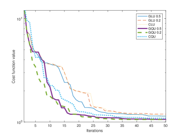
       (i)





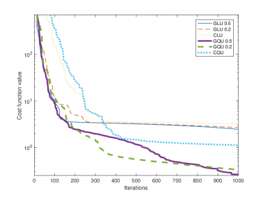
       (ii)






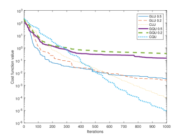
       (iii)





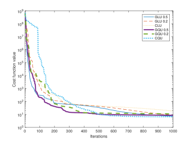
       (iv)



Figure 3: Experimental results for BCD-G algorithms in 9.1.






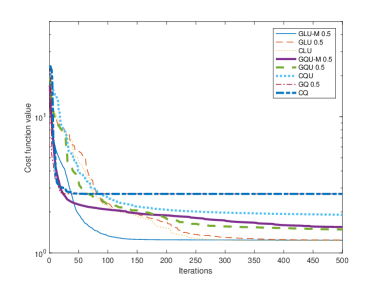
       (i)





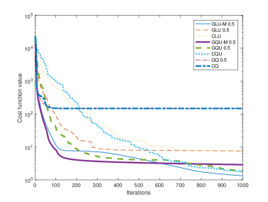
       (ii)



Figure 4: Experimental results for Jacobi-type algorithms in 9.2.


From the above numerical experiments, we can see that: (i) in 9.1, compared with BCD-GLU algorithms, the BCD-GQU algorithms generally have better performances;
(ii) in 9.2, compared with Jacobi-GQU algorithms, the Jacobi-GLU algorithms generally have better performances;
(iii) in 9.2, compared with the Jacobi-GQ and Jacobi-CQ algorithms on $\mathbf{U}_{m}(\mathbb{C})$, the Jacobi-type algorithms on $\mathbf{SL}_{m}(\mathbb{C})$ considered in this paper always obtain much smaller cost function values, and they also need more iterations to attain steady state values of cost functions.



10 Conclusions


In this paper, to solve JADM problem Eq. 1, which is important in BSS problem, we formulate two different equivalent formulations, i.e., problem Eq. 3 defined on $\mathbf{St}(m,n,\mathbb{C})\times\mathbf{SL}_{m}(\mathbb{C})$, and problem Eq. 4 defined on $\mathbf{SL}_{m}(\mathbb{C})$. Then, for these two approaches, based on the Riemannian gradients, we propose three BCD-G algorithms and two Jacobi-G algorithms, and establish their global and weak convergence, under the condition that the iterates are bounded.
An interesting question is, in the BCD-G and Jacobi-G algorithms, whether one can find a method to guarantee both the boundedness of the iterates and the inequalities Eqs. 26 and 27 for global and weak convergence.
If so, then one can get rid of the dependence of convergence results on the condition that the iterates are bounded.



Appendix A Proofs in Section 5



Before the proof of Lemma 5.1, we need to show a lemma, which is similar as equation Eq. 24 and can be directly obtained from [3, Eq. (3.31)].



Lemma A.1.


Let $\exp:\mathbb{C}^{2\times 2}\to\mathbf{GL}_{2}(\mathbb{C})$
be the matrix exponential function [3, 8, 20] sending $\boldsymbol{\Delta}$ to
$\exp(\boldsymbol{\Delta})$.



(i) If $h:\mathbf{SU}_{2}(\mathbb{C})\to\mathbb{R}$ is a differentiable function and $\boldsymbol{\Delta}\in\mathfrak{su}_{2}(\mathbb{C})=\mathbf{T}_{\boldsymbol{I}_{2}}{\mathbf{SU}_{2}(\mathbb{C})}$, we have that



(66)

$$\langle\boldsymbol{\Delta},\mathop{{\operator@font grad}}h(\boldsymbol{I}_{2})\rangle_{\boldsymbol{I}_{2}}=\left.\left(\frac{d}{dt}h(\exp(t\boldsymbol{\Delta}))\right)\right|_{t=0}.$$



(ii) If $h:\mathbf{SUT}_{2}(\mathbb{C})\to\mathbb{R}$ is a differentiable function and $\boldsymbol{\Delta}\in\mathfrak{sut}_{2}(\mathbb{C})=\mathbf{T}_{\boldsymbol{I}_{2}}{\mathbf{SUT}_{2}(\mathbb{C})}$, we have the relationship Eq. 66. 
(iii) If $h:\mathbf{SLT}_{2}(\mathbb{C})\to\mathbb{R}$ is a differentiable function and $\boldsymbol{\Delta}\in\mathfrak{slt}_{2}(\mathbb{C})=\mathbf{T}_{\boldsymbol{I}_{2}}{\mathbf{SLT}_{2}(\mathbb{C})}$, we have the relationship Eq. 66.
(iv) If $h:\mathbf{D}_{2}(\mathbb{C})\to\mathbb{R}$ is a differentiable function and $\boldsymbol{\Delta}\in\mathfrak{d}_{2}(\mathbb{C})=\mathbf{T}_{\boldsymbol{I}_{2}}{\mathbf{D}_{2}(\mathbb{C})}$, we have the relationship Eq. 66.




Proof A.2 (Proof of Lemma 5.1).


Define a projection operator $\mathcal{P}_{i,j}:\mathbb{C}^{m\times m}\to\mathbb{C}^{2\times 2}$ extracting a submatrix of $\boldsymbol{X}\in\mathbb{C}^{m\times m}$ as in [45, Eq. (3.7)], and $\mathcal{P}_{i,j}^{{\sf T}}:\mathbb{C}^{2\times 2}\to\mathbb{C}^{m\times m}$ the conjugate operator.
For the elementary function $h^{(Q)}_{(i,j),\boldsymbol{X}}$ defined in Eq. 38, if $\boldsymbol{\Delta}\in\mathfrak{su}_{2}(\mathbb{C})=\mathbf{T}_{\boldsymbol{I}_{2}}{\mathbf{SU}_{2}(\mathbb{C})}$, we have that




$$\langle\boldsymbol{\Delta},\mathop{{\operator@font grad}}h^{(Q)}_{(i,j),\boldsymbol{X}}(\boldsymbol{I}_{2})\rangle_{\boldsymbol{I}_{2}}=\left.\left(\frac{d}{dt}h^{(Q)}_{(i,j),\boldsymbol{X}}(\exp(t\boldsymbol{\Delta}))\right)\right|_{t=0}\ \ (\text{by \lx@cref{creftypecap~refnum}{lem:gra_rela_elem}(i)})$$




$$=\left.\left(\frac{d}{dt}g(\boldsymbol{X}\boldsymbol{Q}^{(i,j,\exp(t\boldsymbol{\Delta}))})\right)\right|_{t=0}=\left.\left(\frac{d}{dt}g(\text{Exp}_{\boldsymbol{X}}(\boldsymbol{X}\mathcal{P}_{i,j}^{{\sf T}}(\boldsymbol{\Delta})t))\right)\right|_{t=0}$$




$$=\langle\boldsymbol{X}\mathcal{P}_{i,j}^{{\sf T}}(\boldsymbol{\Delta}),\mathop{{\operator@font grad}}g(\boldsymbol{X})\rangle_{\boldsymbol{X}}\ \ (\text{by equation}\ \lx@cref{creftype~refnum}{eq:gradient_exp_map})=\langle\boldsymbol{\Delta},\mathcal{P}_{i,j}(\boldsymbol{\Lambda})\rangle_{\boldsymbol{I}_{2}},$$



where $\text{Exp}_{\boldsymbol{X}}$ is the map defined in Eq. 23.
Note that $\boldsymbol{\Delta}\in\mathfrak{su}_{2}(\mathbb{C})$ and $\mathop{{\operator@font grad}}h^{(Q)}_{(i,j),\boldsymbol{X}}(\boldsymbol{I}_{2})\in\mathfrak{su}_{2}(\mathbb{C})$.
The result can be obtained by direct calculations.
For other three elementary functions $h^{(U)}_{(i,j),\boldsymbol{X}}$, $h^{(L)}_{(i,j),\boldsymbol{X}}$ and $h^{(D)}_{(i,j),\boldsymbol{X}}$, similar as the above case, we can obtain the results by Lemma A.1(ii), Lemma A.1(iii) and Lemma A.1(iv), respectively.
The proof is complete.




We need a simple lemma before the proofs of Proposition 5.3 and Proposition 5.4.



Lemma A.3.


(i) If $z_{1},z_{2}\in\mathbb{C}$,
then




$$|z_{1}-z_{2}|^{2}+|z_{2}|^{2}\geq\frac{3-\sqrt{5}}{2}(|z_{1}|^{2}+|z_{2}|^{2}).$$



(ii) If $\{z_{i}\}_{1\leq i\leq m}\subseteq\mathbb{C}$ satisfy $\sum_{1\leq i\leq m}z_{i}=0$,
then




$$\sum_{1\leq i<j\leq m}|z_{i}-z_{j}|^{2}=m\sum_{1\leq i\leq m}|z_{i}|^{2}.$$








Proof A.4 (Proof of Proposition 5.3).


(i) We first prove the existence of such an index pair $(i_{k},j_{k})$ and an elementary function $h_{k}$ in b 3.
By Lemma 5.2, Lemma A.3 and $\boldsymbol{\Lambda}=\boldsymbol{\Lambda}(\boldsymbol{X}_{k-1})\in\mathfrak{sl}_{m}(\mathbb{C})$, we have that




$$\sum_{1\leq i_{k}<j_{k}\leq m}\left(\|\partial h^{(U)}_{k}(\boldsymbol{I}_{2})\|^{2}+\|\partial h^{(L)}_{k}(\boldsymbol{I}_{2})\|^{2}+\|\partial h^{(D)}_{k}(\boldsymbol{I}_{2})\|^{2}\right)$$




$$=\sum_{1\leq i_{k}<j_{k}\leq m}\left(|\Lambda_{i_{k}j_{k}}|^{2}+|\Lambda_{j_{k}i_{k}}|^{2}\right)+m\sum_{1\leq i_{k}\leq m}|\Lambda_{i_{k}i_{k}}|^{2}\geq\|\boldsymbol{\Lambda}\|^{2}.$$



Therefore, there exist an index pair $(i_{k},j_{k})$ and an elementary function $h_{k}=h^{(U)}_{k},h^{(L)}_{k}$ or $h^{(D)}_{k}$ such that $\frac{3}{2}m(m-1)\|\partial h_{k}(\boldsymbol{I}_{2})\|^{2}\geq\|\boldsymbol{\Lambda}\|^{2}$.



(ii) We now prove the existence in b 4.
Similar as above,
we get that




$$\sum_{1\leq i_{k}<j_{k}\leq m}\left(\|\partial h^{(Q)}_{k}(\boldsymbol{I}_{2})\|^{2}+\|\partial h^{(U)}_{k}(\boldsymbol{I}_{2})\|^{2}+\|\partial h^{(D)}_{k}(\boldsymbol{I}_{2})\|^{2}\right)$$




$$=\sum_{1\leq i_{k}<j_{k}\leq m}\left(|\Lambda_{i_{k}j_{k}}^{*}-\Lambda_{j_{k}i_{k}}|^{2}+|\Lambda_{i_{k}j_{k}}|^{2}+|\Lambda_{i_{k}i_{k}}-\Lambda_{j_{k}j_{k}}|^{2}\right)$$




$$\geq\frac{3-\sqrt{5}}{2}\sum_{1\leq i_{k}<j_{k}\leq m}\left(|\Lambda_{i_{k}j_{k}}|^{2}+|\Lambda_{j_{k}i_{k}}|^{2}\right)+m\sum_{1\leq i_{k}\leq m}|\Lambda_{i_{k}i_{k}}|^{2}\geq\frac{3-\sqrt{5}}{2}\|\boldsymbol{\Lambda}\|^{2}.$$



Therefore, there exists an index pair $(i_{k},j_{k})$ and an elementary function $h_{k}=h^{(Q)}_{k},h^{(U)}_{k}$ or $h^{(D)}_{k}$ such that
$\frac{3}{3-\sqrt{5}}m(m-1)\|\partial h_{k}(\boldsymbol{I}_{2})\|^{2}\geq\|\boldsymbol{\Lambda}\|^{2}.$
The proof is complete.




Proof A.5 (Proof of Proposition 5.4).


Note that the starting point $\boldsymbol{X}_{0}\in\mathbf{EUT}_{m}(\mathbb{C})$ in b 5.
We see that $\boldsymbol{X}_{k}\in\mathbf{EUT}_{m}(\mathbb{C})$ for all $k\in\mathbb{N}$.
By Lemma 5.2, Lemma A.3 and $\boldsymbol{\Lambda}=\boldsymbol{\Lambda}(\boldsymbol{X}_{k-1})\in\mathfrak{eut}_{m}(\mathbb{C})$, we get that




$${\small\sum_{1\leq i_{k}<j_{k}\leq m}\left(\|\partial h^{(U)}_{k}(\boldsymbol{I}_{2})\|^{2}+\|\partial h^{(D)}_{k}(\boldsymbol{I}_{2})\|^{2}\right)}
{\small=\sum_{1\leq i_{k}<j_{k}\leq m}\left(|\Lambda_{i_{k}j_{k}}|^{2}+|\Lambda_{i_{k}i_{k}}-\Lambda_{j_{k}j_{k}}|^{2}\right)}$$






$${\small=\sum_{1\leq i_{k}<j_{k}\leq m}|\Lambda_{i_{k}j_{k}}|^{2}+m\sum_{1\leq i_{k}\leq m}|\Lambda_{i_{k}i_{k}}|^{2}\geq\|\boldsymbol{\Lambda}\|^{2}.}$$



Therefore, there exist an index pair $(i_{k},j_{k})$ and an elementary function $h_{k}=h^{(U)}_{k}$ or $h^{(D)}_{k}$ such that
$m(m-1)\|\partial h_{k}(\boldsymbol{I}_{2})\|^{2}\geq\|\boldsymbol{\Lambda}\|^{2}$.
The proof is complete.






Appendix B Proofs in Section 6




Proof B.1 (Proof of Lemma 6.6).


We now prove the inequality Eq. 46 by Lemma 6.2(iii) in three different cases shown in 6.5.


 

If $\gamma_{1}=\gamma_{2}=0$, it is clear that the inequality Eq. 46 is satisfied for any $\iota_{D}>0$






 

If $\varpi\in[0,\varsigma_{D})$, we get that




$$h^{(D)}_{k}(1,0)-h^{(D)}_{k}(x_{k}^{*},y_{k}^{*})=\frac{3}{4}\gamma_{1}(1-4\varpi)=\frac{3(1-4\varpi)}{8(1-\varpi)}|\partial h^{(D)}_{k}(1,0)|$$




$$\geq\frac{3(1-4\varpi)\varepsilon}{8(1-\varpi)}\|\boldsymbol{\Lambda}(\boldsymbol{X}_{k-1})\|=\frac{3(1-4\varpi)\varepsilon}{4\sqrt{5}(1-\varpi)}\frac{\sqrt{5}}{2}\|\boldsymbol{\Lambda}(\boldsymbol{X}_{k-1})\|$$




$$\geq\frac{3(1-4\varpi)\varepsilon}{4\sqrt{5}(1-\varpi)}\|\boldsymbol{\Lambda}(\boldsymbol{X}_{k-1})\|\|\boldsymbol{\Psi}^{*}_{k}-\boldsymbol{I}_{2}\|\geq\frac{3(1-4\varsigma_{D})\varepsilon}{4\sqrt{5}}\|\boldsymbol{\Lambda}(\boldsymbol{X}_{k-1})\|\|\boldsymbol{\Psi}^{*}_{k}-\boldsymbol{I}_{2}\|.$$




 

If $\varpi\in(\frac{1}{\varsigma_{D}},+\infty]$, we similarly get the above inequality.

• 

If $\varpi\in[\varsigma_{D},\frac{1}{\varsigma_{D}}]$,
it is easy to verify that



(67)

$$\sqrt[4]{\gamma_{1}\gamma_{2}}\geq\frac{\sqrt[4]{\varsigma_{D}}}{2}\left(\sqrt{\gamma_{1}}+\sqrt{\gamma_{2}}\right).$$


Then, we get that




$\displaystyle h^{(D)}_{k}(1,0)-h^{(D)}_{k}(x_{k}^{*},y_{k}^{*})=\left(\sqrt{\gamma_{1}}-\sqrt{\gamma_{2}}\right)^{2}=\frac{1}{2}|\partial h^{(D)}_{k}(1,0)|\frac{\left|\sqrt{\gamma_{1}}-\sqrt{\gamma_{2}}\right|}{\sqrt{\gamma_{1}}+\sqrt{\gamma_{2}}}$



$\displaystyle\geq\frac{\varepsilon\sqrt[4]{\varsigma_{D}}}{4}\|\boldsymbol{\Lambda}(\boldsymbol{X}_{k-1})\|\frac{\left|\sqrt{\gamma_{1}}-\sqrt{\gamma_{2}}\right|}{\sqrt[4]{\gamma_{1}\gamma_{2}}}\ \ (\textrm{by equation \lx@cref{creftype~refnum}{eq:inequa_rho_r4_c}})$



$\displaystyle\geq\frac{\varepsilon\sqrt[4]{\varsigma_{D}}}{4}\|\boldsymbol{\Lambda}(\boldsymbol{X}_{k-1})\|\frac{\left|\sqrt[4]{\gamma_{1}}-\sqrt[4]{\gamma_{2}}\right|\left(\sqrt{\gamma_{1}}+\sqrt{\gamma_{2}}\right)^{1/2}}{\sqrt[4]{\gamma_{1}\gamma_{2}}}$



$\displaystyle\geq\frac{\varepsilon\sqrt[4]{\varsigma_{D}}}{4}\|\boldsymbol{\Lambda}(\boldsymbol{X}_{k-1})\||x_{k}^{*}-1|\sqrt{1+\frac{1}{{x_{k}^{*}}^{2}}}\geq\frac{\varepsilon\sqrt[4]{\varsigma_{D}}}{4}\|\boldsymbol{\Lambda}(\boldsymbol{X}_{k-1})\|\|\boldsymbol{\Psi}^{*}_{k}-\boldsymbol{I}_{2}\|.$





Now we set $\iota_{D}=\min(\frac{3(1-4\varsigma_{D})\varepsilon}{4\sqrt{5}},\frac{\varepsilon\sqrt[4]{\varsigma_{D}}}{4})$.
The proof is complete.




Proof B.2 (Proof of Lemma 6.8).


We prove that the inequality Eq. 50 is satisfied in two cases.


 

If $h_{k}=h^{(U)}_{k}$, by Lemma 6.2(i), we see that




$$g(\boldsymbol{X}_{k-1})-g(\boldsymbol{X}_{k})
=h^{(U)}_{k}(0,0)-h^{(U)}_{k}(x_{k}^{*},y_{k}^{*})=\frac{1}{\alpha_{1}}(\alpha_{2}^{2}+\alpha_{3}^{2})$$






$$=\frac{1}{2}\|\partial h^{(U)}_{k}(0,0)\|\|(x_{k}^{*},y_{k}^{*})\|\geq\frac{\varepsilon}{2}\|\boldsymbol{\Lambda}(\boldsymbol{X}_{k-1})\|\|\boldsymbol{\Psi}^{*}_{k}-\boldsymbol{I}_{2}\|.$$






 

If $h_{k}=h^{(L)}_{k}$, by Lemma 6.2(ii), we see that




$$g(\boldsymbol{X}_{k-1})-g(\boldsymbol{X}_{k})
=h^{(L)}_{k}(0,0)-h^{(L)}_{k}(x_{k}^{*},y_{k}^{*})=\frac{1}{\beta_{1}}(\beta_{2}^{2}+\beta_{3}^{2})$$






$$=\frac{1}{2}\|\partial h^{(L)}_{k}(0,0)\|\|(x_{k}^{*},y_{k}^{*})\|\geq\frac{\varepsilon}{2}\|\boldsymbol{\Lambda}(\boldsymbol{X}_{k-1})\|\|\boldsymbol{\Psi}^{*}_{k}-\boldsymbol{I}_{2}\|.$$






Now we set $\iota_{LU}=\frac{\varepsilon}{2}$. The proof is complete.







Proof B.3 (Proof of Lemma 6.10).


If $h_{k}=h^{(U)}_{k}$, we have




$$\|\boldsymbol{\Psi}^{*}_{k}-\boldsymbol{I}_{2}\|^{2}=\frac{\alpha_{2}^{2}+\alpha_{3}^{2}}{\alpha_{1}^{2}}\geq\frac{\|\partial h^{(U)}_{k}(0,0)\|^{2}}{4\mathrm{M}_{\alpha}^{2}}\geq\frac{\varepsilon^{2}}{4\mathrm{M}_{\alpha}^{2}}\|\boldsymbol{\Lambda}(\boldsymbol{X}_{k-1})\|^{2},$$



where $\mathrm{M}_{\alpha}$ is a fixed positive constant always satisfying $|\alpha_{1}|\leq\mathrm{M}_{\alpha}$.
The case $h_{k}=h^{(L)}_{k}$ is similar.
Now we prove the $h_{k}=h^{(D)}_{k}$ case. If $\varpi\in[0,\varsigma_{D})$, we have that




$$\|\boldsymbol{\Psi}^{*}_{k}-\boldsymbol{I}_{2}\|^{2}=\frac{5}{4}\geq\frac{5}{4}\frac{1}{4(\gamma_{1}^{2}+\gamma_{2}^{2})}\|\partial h^{(D)}_{k}(1,0)\|^{2}\geq\frac{5}{4}\frac{\varepsilon^{2}}{4\mathrm{M}_{0}^{2}}\|\boldsymbol{\Lambda}(\boldsymbol{X}_{k-1})\|^{2}.$$



The case $\varpi\in(\frac{1}{\varsigma_{D}},+\infty]$ is similar.
If $\varpi\in[\varsigma_{D},\frac{1}{\varsigma_{D}}]$, we have




$$\|\boldsymbol{\Psi}^{*}_{k}-\boldsymbol{I}_{2}\|^{2}\geq(1-x_{k}^{*})^{2}\geq\frac{\gamma_{1}^{2}(1-\varpi)^{2}}{\mathrm{M}_{0}^{2}\mathrm{M}_{\varpi}^{2}}=\frac{\|\partial h^{(D)}_{k}(1,0)\|^{2}}{4\mathrm{M}_{0}^{2}\mathrm{M}_{\varpi}^{2}}\geq\frac{\varepsilon^{2}}{4\mathrm{M}_{0}^{2}\mathrm{M}_{\varpi}^{2}}\|\boldsymbol{\Lambda}(\boldsymbol{X}_{k-1})\|^{2},$$



where $\mathrm{M}_{\varpi}$ is a fixed positive constant always satisfying $(1+\sqrt{\varpi})(1+\sqrt[4]{\varpi})\leq\mathrm{M}_{\varpi}$.
We only need to set $\kappa^{2}$ to be the minimum of all the above corresponding positive constants.
The proof is complete.






Acknowledgment


The authors would like to thank the three anonymous reviewers and the editor for their helpful suggestions and comments, which significantly improved the presentation of the article.

References

[1]T. E. Abrudan, J. Eriksson, and V. Koivunen, Steepest descent
algorithms for optimization under unitary matrix constraint, IEEE
Transactions on Signal Processing, 56 (2008), pp. 1134–1147.
[2]P.-A. Absil, R. Mahony, and B. Andrews, Convergence of the iterates
of descent methods for analytic cost functions, SIAM Journal on
Optimization, 16 (2005), pp. 531–547.
[3]P.-A. Absil, R. Mahony, and R. Sepulchre, Optimization algorithms on
matrix manifolds, Princeton University Press, 2009.
[4]B. Afsari, Gradient flow-based matrix joint diagonalization for
independent component analysis, University of Maryland, College Park, 2004.
Master’s thesis.
[5]B. Afsari, Simple LU and QR based non-orthogonal matrix joint
diagonalization, in International Conference on Independent Component
Analysis and Signal Separation, Springer, 2006, pp. 1–7.
[6]B. Afsari, What can make joint diagonalization difficult?, in
ICASSP, vol. III, Honolulu, Apr. 2007, pp. 1377–1380.
[7]R. André, X. Luciani, and E. Moreau, A new class of block
coordinate algorithms for the joint eigenvalue decomposition of complex
matrices, Signal Processing, 145 (2018), pp. 78–90.
[8]A. Baker, Matrix groups: An introduction to Lie group theory,
Springer Science & Business Media, 2012.
[9]D. P. Bertsekas, Nonlinear programming, Athena Scientific,
second ed., 1999.
[10]F. Bouchard, B. Afsari, J. Malick, and M. Congedo, Approximate joint
diagonalization with Riemannian optimization on the general linear group,
SIAM Journal on Matrix Analysis and Applications, 41 (2020), pp. 152–170.
[11]D. Brandwood, A complex gradient operator and its application in
adaptive array theory, IEE Proceedings H-Microwaves, Optics and Antennas,
130 (1983), pp. 11–16.
[12]J. Cardoso and A. Souloumiac, Blind beamforming for non-gaussian
signals, IEE Proceedings F (Radar and Signal Processing), 6 (1993),
pp. 362–370.
[13]J.-F. Cardoso and A. Souloumiac, Jacobi angles for simultaneous
diagonalization, SIAM Journal on Matrix Analysis and Applications, 17
(1996), pp. 161–164.
[14]G. Chabriel, M. Kleinsteuber, E. Moreau, H. Shen, P. Tichavsky, and
A. Yeredor, Joint matrices decompositions and blind source separation:
A survey of methods, identification, and applications, IEEE Signal
Processing Magazine, 31 (2014), pp. 34–43.
[15]B. Chen, S. He, Z. Li, and S. Zhang, Maximum block improvement and
polynomial optimization, SIAM Journal on Optimization, 22 (2012),
pp. 87–107.
[16]P. Comon, Independent Component Analysis, in Higher Order
Statistics, J.-L. Lacoume, ed., Elsevier, Amsterdam, London, 1992,
pp. 29–38.
[17]P. Comon, Independent component analysis, a new concept?, Signal
Processing, 36 (1994), pp. 287–314.
[18]P. Comon and C. Jutten, eds., Handbook of Blind Source Separation,
Academic Press, Oxford, 2010.
[19]G. Golub and C. Van Loan, Matrix Computations, Johns Hopkins
University Press, third ed., 1996.
[20]B. Hall, Lie groups, Lie algebras, and representations: an
elementary introduction, vol. 222, Springer, 2015.
[21]M. Ishteva, P.-A. Absil, and P. Van Dooren, Jacobi algorithm for
the best low multilinear rank approximation of symmetric tensors, SIAM
Journal on Matrix Analysis and Applications, 2 (2013), pp. 651–672.
[22]S. Krantz and H. Parks, A Primer of Real Analytic Functions,
Birkhäuser Boston, 2002.
[23]S. G. Krantz, Function theory of several complex variables,
vol. 340, American Mathematical Soc., 2001.
[24]S. law Lojasiewicz, Ensembles semi-analytiques, IHES notes,
(1965).
[25]J. Li, K. Usevich, and P. Comon, Globally convergent Jacobi-type
algorithms for simultaneous orthogonal symmetric tensor diagonalization,
SIAM Journal on Matrix Analysis and Applications, 39 (2018), pp. 1–22.
[26]J. Li, K. Usevich, and P. Comon, On approximate diagonalization of
third order symmetric tensors by orthogonal transformations, Linear Algebra
and its Applications, 576 (2019), pp. 324–351.
[27]J. Li, K. Usevich, and P. Comon, On the convergence of jacobi-type
algorithms for independent component analysis, in 2020 IEEE 11th Sensor
Array and Multichannel Signal Processing Workshop (SAM), IEEE, 2020,
pp. 1–5.
[28]J. Li, K. Usevich, and P. Comon, Jacobi-type algorithm for low rank
orthogonal approximation of symmetric tensors and its convergence analysis,
Pacific Journal of Optimization, 17 (2021), pp. 357–379.
[29]J. Li and S. Zhang, Polar decomposition based algorithms on the
product of Stiefel manifolds with applications in tensor approximation,
Journal of the Operations Research Society of China, (2023).
[30]Z. Li, A. Uschmajew, and S. Zhang, On convergence of the maximum
block improvement method, SIAM Journal on Optimization, 25 (2015),
pp. 210–233.
[31]S. Łojasiewicz, Sur la géométrie semi- et
sous-analytique, Annales de l’institut Fourier, 43 (1993), pp. 1575–1595.
[32]Z.-Q. Luo and P. Tseng, On the convergence of the coordinate descent
method for convex differentiable minimization, Journal of Optimization
Theory and Applications, 72 (1992), pp. 7–35.
[33]Z.-Q. Luo and P. Tseng, Error bounds and convergence analysis of
feasible descent methods: a general approach, Annals of Operations Research,
46 (1993), pp. 157–178.
[34]J. H. Manton, Modified steepest descent and Newton algorithms for
orthogonally constrained optimisation. part i. the complex Stiefel
manifold, in Proceedings of the Sixth International Symposium on Signal
Processing and its Applications, vol. 1, IEEE, 2001, pp. 80–83.
[35]V. Maurandi, C. De Luigi, and E. Moreau, Fast jacobi like algorithms
for joint diagonalization of complex symmetric matrices, in 21st European
Signal Processing Conference (EUSIPCO 2013), IEEE, 2013, pp. 1–5.
[36]V. Maurandi and E. Moreau, A decoupled Jacobi-like algorithm for
non-unitary joint diagonalization of complex-valued matrices, IEEE Signal
Processing Letters, 21 (2014), pp. 1453–1456.
[37]V. Maurandi, E. Moreau, and C. De Luigi, Jacobi like algorithm for
non-orthogonal joint diagonalization of hermitian matrices, in 2014 IEEE
International Conference on Acoustics, Speech and Signal Processing (ICASSP),
IEEE, 2014, pp. 6196–6200.
[38]J. Nocedal and S. Wright, Numerical optimization, Springer Science
& Business Media, 2006.
[39]W. Ring and B. Wirth, Optimization methods on Riemannian manifolds
and their application to shape space, SIAM Journal on Optimization, 22
(2012), pp. 596–627.
[40]H. Sato and T. Iwai, A new, globally convergent Riemannian
conjugate gradient method, Optimization, 64 (2015), pp. 1011–1031.
[41]R. Schneider and A. Uschmajew, Convergence results for projected
line-search methods on varieties of low-rank matrices via łojasiewicz
inequality, SIAM Journal on Optimization, 25 (2015), pp. 622–646.
[42]M. Sørensen, P. Comon, S. Icart, and L. Deneire, Approximate
tensor diagonalization by invertible transforms, in 2009 17th European
Signal Processing Conference, Eurasip, 2009, pp. 500–504.
[43]A. Souloumiac, Nonorthogonal joint diagonalization by combining
givens and hyperbolic rotations, IEEE Transactions on Signal Processing, 57
(2009), pp. 2222–2231.
[44]A. Uschmajew, A new convergence proof for the higher-order power
method and generalizations, Pacific Journal of Optimization, 11 (2015),
pp. 309–321.
[45]K. Usevich, J. Li, and P. Comon, Approximate matrix and tensor
diagonalization by unitary transformations: convergence of jacobi-type
algorithms, SIAM Journal on Optimization, 30 (2020), pp. 2998–3028.
[46]K. Wang, X.-F. Gong, and Q.-H. Lin, Complex non-orthogonal joint
diagonalization based on LU and LQ decompositions, in International
Conference on Latent Variable Analysis and Signal Separation, Springer, 2012,
pp. 50–57.
[47]S. J. Wright, Coordinate descent algorithms, Mathematical
Programming, 151 (2015), pp. 3–34.
[48]Y. Xu and W. Yin, A block coordinate descent method for regularized
multiconvex optimization with applications to nonnegative tensor
factorization and completion, SIAM Journal on Imaging Sciences, 6 (2013),
pp. 1758–1789.
[49]A. Yeredor, Non-orthogonal joint diagonalization in the
least-squares sense with application in blind source separation, IEEE
Transactions on Signal Processing, 50 (2002), pp. 1545–1553.