Replica Analysis of the Linear Model with Markov or Hidden Markov Signal Priors

Abstract

This paper estimates free energy, average mutual information, and minimum mean square error (MMSE) of a linear model under two assumptions: (1) the source is generated by a Markov chain, (2) the source is generated via a hidden Markov model. Our estimates are based on the replica method in statistical physics. We show that under the posterior mean estimator, the linear model with Markov sources or hidden Markov sources is decoupled into single-input AWGN channels with state information available at both encoder and decoder where the state distribution follows the left Perron-Frobenius eigenvector with unit Manhattan norm of the stochastic matrix of Markov chains. Numerical results show that the free energies and MSEs obtained via the replica method are closely approximate to their counterparts achieved by the Metropolis–Hastings algorithm or some well-known approximate message passing algorithms in the research literature.

I Introduction

In the canonical compressed sensing problem, the primary goal is to reconstruct an $n$-dimensional vector $\bm{X}=(X_{1},X_{2},\cdots,X_{n})$ with independent and identical prior from an $m$-dimensional vector of noisy linear observations $\bm{Y}=(Y_{1},Y_{2},\cdots,Y_{m})$ of the form $Y_{k}=\langle\bm{\Phi}_{k},\bm{X}\rangle+W_{k},k=1,2,\cdots,m$, where $\{\bm{\Phi}_{k}\}$ is a sequence of $n$-dimensional measurement vectors, $\{W_{k}\}$ is a sequence of standard Gaussian random variables, and $\langle\cdot,\cdot\rangle$ denotes the Euclidean inner product between vectors. In this paper, under the assumption that $\bm{X}$ has a Markov or hidden Markov prior, we wish to estimate the asymptotic mutual information $\lim_{n\to\infty}\frac{1}{n}I(\bm{X};\bm{Y})$ and the MMSE $\lim_{n\to\infty}\frac{1}{n}\mathbb{E}[\|\bm{X}-\mathbb{E}[\bm{X}|\bm{Y},\bm{\Phi}]\|^{2}]$. Our estimates are based on the replica method which was developed originally to study mean field approximations in spin glasses [1]. Although this method lacks of rigorous mathematical proof in some particular parts, it has been widely accepted as an analytic tool and utilized to investigate a variety of problems in applied mathematics, information processing, machine learning, and coding [2].

I-A Related Work

The use of the replica method for studying multiuser estimators goes back to [3] where Tanaka determined the asymptotic bit error rate of Marginal-Posterior-Mode (MPM) estimators by employing the replica method. The study demonstrated interesting large-system properties of multiuser estimators. As a result, the statistical physics approach received more attention in the context of multiuser systems [4, 5] with a subsequent work focusing on the compressed sensing directly [6, 7, 8, 9, 10, 11]. Guo and Verdú [4] studied the same CDMA detection problem as [3] but under more general (arbitrary) input distributions. They assumed that a generic posterior mean estimator is applied before single-user decoding. The generic detector can be particularized to the matched filter, decorrelator, linear minimum mean-square error (MMSE) detector, the jointly or the individual optimal detector, and others. It is found that the detection output for each user, although in general asymptotically non-Gaussian conditioned on the transmitted symbol, converges as the number of users go to infinity to a deterministic function of a “hidden” Gaussian statistic independent of the interferers. Thus, the multi-user channel can be decoupled.

The results of replica method have been rigorously in a number of settings in compressed sensing. One example is given by message passing on matrices with special structure, such as sparsity [12, 13, 14, 15, 16] or spatial coupling [17, 18, 19]. In [8], Rangan et al. studied the asymptotic performance of a class of Maximize-A-Posterior (MAP) estimators. Using standard large deviation techniques, the authors represented the MAP estimator as the limit of an indexed MMSE estimator’s sequence. Consequently, they determined the estimator’s asymptotics employing the results from [4] and justified the decoupling property of MAP estimators under Replica Symmetry (RS) assumption for an i.i.d. measurement matrix $\bm{\Phi}$. The asymptotic performance for the MAP estimator where the RS assumption does not hold but satisfies some looser symmetric assumptions, called Replica Symmetry Breaking (RSB) is considered in [2]. Under the RSB assumption with $b$ steps of breaking (bRSB), the equivalent noisy single-user channel is given in form of an input term added by an impairment term. The impairment term, moreover, is expressed as a sum of an independent Gaussian random variable and $b$ correlated non-Gaussian interference terms.

Recently, there have been some works which aim to close the gap between mathematically rigorous proof and results from the replica method. Reeves and Pfister considered the fundamental limit of compressed sensing for i.i.d. signal distributions and i.i.d. Gaussian measurement matrices [20]. Under some mild technical conditions, their results show that the limiting mutual information and Minimum Mean Square Error (MMSE) are equal to the values predicted by the replica method. Their proof techniques are based on establishing relationships between mutual information and MMSE at finite $n,m$ and $n\sim m$ such as [21], and extending obtained results in large system limits. In [22], Barbier et al. showed that the results for Generalized Linear Models (GLM) and i.i.d. sources stemming from the replica method are indeed correct and imply the optimal value of both estimation and generalization error. The proof is based on the adaptive interpolation method [23] which is an extension of interpolation method developed by Guerra and Toninelli [24] in the context of spin glasses, with an adaptive interpolation path. More specifically, this scheme interpolates between the original problem and the solution via replica method in small steps, each step involving its own set of trial parameters and Gaussian mean-fields in the spirit of Guerra and Toninelli. We are then able to choose the set of trial parameters in various ways so that the upper and lower bounds are eventually matched. By a generalization of the adaptive interpolation method, Truong [25] has recently established exact asymptotic expressions for the normalized mutual information and MMSE of sparse linear regression in the sub-linear sparsity regime, i.e., $m=n^{\alpha}$ for some $\alpha\in(0,1)$. This work shows that the traditional linear assumption between the signal dimension and number of observations in the replica and adaptive interpolation methods is not necessary for sparse signals.

In all above research literature, the authors assume that the source is independently and identically distributed (i.i.d.). In many practical applications, samples of input data may be dependent on each other, e.g., Markov chains or hidden Markov models. There are a few non-rigorous literatures handling Markov chains using the replica method [26, 27, 28]. However, to the best of our knowledge, there exists no rigorously analytic result which was developed based on replica-related methods for these models. Some recent works considered the linear model with random generative priors where the signal is the output of a Bayesian neural network with specific structures with the input being an i.i.d. sequence [29, 30, 31]. Although these papers are to recover the structured signal, however, the signal structure is different from Markov or hidden Markov. For example, if we use a classifier (one layer neural network) with ReLU activation function, i.e., $\bm{x}=\sigma(\bm{a}^{T}\bm{u})$ where $\bm{a}$ is Gaussian as the assumptions in these papers and $\bm{u}$ is an i.i.d. vector, then $\bm{x}$ is not Markov or Hidden Markov. The adaptive interpolation method looks hard to apply for the linear model with Markov sources or hidden Markov sources since it requires that $X_{1},X_{2},\ldots,X_{n}$ are i.i.d. (or at least i.i.d. block-by-block) to guarantee a fixed interpolating free energy at the final $(k,t)$-interpolation model for each finite value of $n$ [23]. There were also some existing works related to Mean Square Errors (MSE) achieved by Approximate Message Passing algorithms (AMP) for the linear model with Markov or hidden Markov sources [32, 33, 34]. Approximate message passing (AMP) refers to a class of efficient algorithms for statistical estimation in high-dimensional problems such as compressed sensing and low-rank matrix estimation. AMP is initially proposed for sparse signal recovery and compressed sensing [35, 36, 37]. AMP algorithms have been proved to be effective in reconstructing sparse signals from a small number of incoherent linear measurements. Their dynamics are accurately tracked by a simple one-dimensional iteration termed state evolution [38]. The state evolution is redefined in non-asymptotic sense for the sparse linear regression with sublinear sparsity in [25]. AMP algorithms achieve state-of-the-art performance for several high-dimensional statistical estimation problems, including compressed sensing [39, 38, 18] and low-rank matrix estimation [38, 40].

I-B Main Contributions

In this paper, based on the same replica assumptions as [4], we establish free energy, mutual information, and MMSE for the linear model with Markov or hidden Markov sources. When limiting to the linear model with i.i.d. sources as case, we recover Guo and Verdú’s results [4], which extends Tanaka work [3] to more general alphabets. More specially, our main contributions are as follows:

• Using the replica method, we estimate the free energy, the normalized mutual information in the large system limit for two models: linear model with Markov sources and linear model with hidden Markov sources (cf. Claim 1 and Claim 3).

• Using the replica method, we characterize MMSEs in the large system limit for two estimation problems (cf. Claim 2 and Claim 3). We show that under the posterior mean estimator, the linear model with Markov sources or hidden Markov sources is decoupled into single-input AWGN channels with state information available at both encoder and decoder where the state distribution follows the left Perron-Frobenius eigenvector with unit Manhattan norm of the stochastic matrix of Markov chains.

• We show that the free energies and MSEs obtained via the replica method are closely approximate to their counterparts achieved by the Metropolis–Hastings algorithm or some well-known approximate message passing algorithms in the research literature (cf. Section IV).

Essentially, our results show that in the large system limit, we can convert the estimation in high-dimensional space for the linear model with Markov or hidden Markov signal prior to the estimation problems in one-dimensional spaces. Compared with the linear model with i.i.d. sources [4], we need to deal with some new technical challenges related to the estimation of the derivative of Perron-Frobenius eigenvalue of non-negative matrices. For example, in the following Lemma 7, we develop a new technique to estimate this derivative in the large system limit.

MMSE and free energy are very important fundamental limits, which are benchmarks to check if a coding scheme or a learning algorithm for the linear model is optimal. In this work, we aim to characterize these fundamental limits by using replica method. Our simulation results (cf. Section IV) show that some existing MCMC algorithms (for example, Metropolis–Hastings algorithm) and AMP (for example, Turbo AMP [32]) are (potentially) optimal for the linear model with Markov or hidden Markov signal prior. Before our work, whether these interesting algorithms are optimal or not is an open question.

I-C Paper Organization

The problem setting is placed in Section II, where we introduce the system model, posterior mean estimation, free energy and replica method in statistical physics. We also introduce some new concepts such as single-symbol Posterior Mean Estimation (PME) channel with state information, free energy functions, and other related notations in this section. Our main results are stated and proved in Section III. We apply our main results to estimate free energy, mutual information, and MMSE for some specific Markov chains or hidden Markov models in Section IV, where we also compare our obtained MMSEs with achievable MSEs by the classical Metropolis–Hastings algorithm and some well-known AMP algorithms in research literature. In Appendix A, we introduce some related results on large deviations and develop new ones for specific applications in this paper. Appendix B begins with some results on Perron-Frobenius eigenvalues, and ends with an estimation of the derivative of the Perron-Frobenius eigenvalue for a Markov chain formed by covariance matrices. The proof of joint moments in Section III is placed in Appendix C since the proof technique is similar to the proof of another theorem in Section III. Appendix D provides extensions to Markov chains on a general Polish space in $\mathbb{R}$.

I-D Notation

Use $[n]$ to denote the set $\{1,\ldots,n\}$. Random vectors and matrices are in bold letters. Expectations with respect to “quenched” random variables (i.e., the variables that are fixed by the realization of the problem) are denoted by $\mathbb{E}$ and those with respect to “annealed” random variables (i.e., dynamical variables) are denoted by Gibbs bracket $\langle-\rangle$ possibly with appropriate subscripts. This choice follows the stardards of statistical physics.

As standard literature, we define $x^{n}=(x_{1},x_{2},\cdots,x_{n})^{T}$ to denote a vector of length $n$. However, if the dimension of a vector $x$ is clear from context, we omit it for simplicity. Define two loss functions $l_{1}:\mathbb{R}\times\mathbb{R}\to\mathbb{R}$ and $l_{2}:\mathbb{R}\times\mathbb{R}\to\mathbb{R}$ as $l_{1}(x,y)=|x-y|$ and $l_{2}(x,y)=(x-y)^{2}$. Let $\log x:=\log_{2}x$ and $\ln x$ be the natural logarithm of $x$ for all $x\in\mathbb{R}^{+}$. Manhattan and Euclidean norms of a vector $x\in\mathbb{R}^{n}$ are defined as

$$\|x\|_{1} :=\sum_{i=1}^{n}|x_{i}|,$$ (1)

$$\|x\|_{2} :=\sqrt{\sum_{i=1}^{n}|x_{i}|^{2}},$$ (2)

respectively. In addition, $\rm{vec}(\cdot)$ denotes the vectorization operator. Besides, for any $A\in\mathbb{R}^{p\times q}$ and $B\in(\mathbb{R}^{n\times n})^{p\times q}$, we define $Ao_{\mathrm{tr}}B:=\sum_{i,j}A_{ij}\odot B_{ij}$, where $A\odot B$ is the Hadamard product between $A$ and $B$.

The moment generating function of a random vector $\bm{X}\in\mathbb{R}^{n}$ is defined as $\mathcal{M}(\lambda):=\mathbb{E}[\exp(\lambda^{T}\bm{X})]$ for all $\lambda\in\mathbb{R}^{n}$. Let $\mathcal{M}(\tilde{Q}):=\mathbb{E}[\exp(\mathrm{tr}(\tilde{Q}\bm{Q}))]$ be the moment generating function of a random matrix $\bm{Q}\in\mathbb{R}^{n\times n}$ for all matrix $\tilde{Q}\in\mathbb{R}^{n\times n}$.

Denote by

$$\mathcal{Q}:=\bigg{\{}sxx^{T}\enspace\mbox{for some}\enspace x\in\mathcal{S}\times\mathcal{X}^{\nu+1}\bigg{\}}.$$ (3)

For simplicity of presentation, we enumerate all matrices in $\mathcal{Q}$ as $\bar{Q}_{0},\bar{Q}_{1},\cdots,\bar{Q}_{M}$ where $M:=|\mathcal{Q}|-1$.

II Problem Setting

We consider the linear model

$$\bm{Y}=\bm{\Phi}\bm{X}+\bm{W}=\bm{A}\bm{S}^{1/2}\bm{X}+\bm{W}.$$ (4)

Here $\bm{Y}\in\mathbb{R}^{m}$ is a vector of observations, $\bm{X}\in\mathbb{R}^{n}$ is the signal vector, $\bm{A}\in\mathbb{R}^{m\times n}$ is a measurement matrix, $\bm{S}$ is diagonal matrix of positive scale factors:

$$\bm{S}=\operatorname{diag}(S_{1},S_{2},\cdots,S_{n}),\quad S_{j}\in\mathbb{R}^{+},$$ (5)

and $\bm{W}\in\mathbb{R}^{m}$ is a noise vector. We consider a sequence of problems indexed by $n$, and make the following assumptions on the model. These assumptions are identical to those in earlier works [4, 8] except for the signal prior, which we allow to be Markov or hidden Markov in contrast to the i.i.d. priors considered in earlier works.

1. We assume that the number of measurements $m$ scales linearly with $n$, and $\lim_{n\to\infty}\frac{n}{m}=\beta$, for some $\beta>0$.

2. The elements $\{A_{ij}\}_{i\in[m],j\in[n]}$ of the matrix $\bm{A}$ are i.i.d. and distributed as $A_{ij}\stackrel{{\scriptstyle\text{d}}}{{=}}\frac{1}{\sqrt{m}}A$, where $A$ is a random variable with zero mean, unit variance and all moments finite.

3. The scale factors $(S_{1},\ldots,S_{n})$ are i.i.d. according to $P_{S}$, which is supported on a set $\mathcal{S}\subset\mathbb{R}^{+}$. The scale factors $(S_{1},\ldots,S_{n})$ are independent of $\bm{A},\bm{X}$, and $\bm{W}$.

4. The noise vector $\bm{W}$ is standard normal, i.e., $W_{j}\sim_{\text{i.i.d.}}\mathcal{N}(0,1)$ for $j\in[m]$.

5. Signal prior: We assume that the components of $\bm{X}$ take values on a Polish space on $\mathbb{R}$, and are distributed according to either a Markov or a hidden Markov prior.

   • Markov chain prior: This model assumes that

     $$\mathbb{P}(\bm{X}=(x_{1},\ldots,x_{n}))=p(x_{1})\pi(x_{1},x_{2})\cdots\pi(x_{n-1},x_{n})$$ (6)

     for some initial probability distribution $p(\cdot)$ on $\mathcal{X}$, where $\pi(\cdot,\cdot)$ is the transition probability of a time-homogeneous, irreducible Markov chain on $\mathcal{X}$.

   • Hidden Markov prior: The second model assumes that $\{X_{n}\}_{n=1}^{\infty}$ are generated by a Hidden Markov Model (HMM), with hidden states $\{\Upsilon_{n}\}_{n=1}^{\infty}$ take values on a Polish space on $\mathcal{H}_{\Upsilon}$. That is, $\mathbb{P}(\bm{\Upsilon}=(\upsilon_{1},\ldots,\upsilon_{n}))=p_{\Upsilon}(\upsilon_{1})\pi_{\Upsilon}(\upsilon_{1},\upsilon_{2})\cdots\pi_{\Upsilon}(\upsilon_{n-1},\upsilon_{n})$ for some initial probability distribution $p_{\Upsilon}(\cdot)$ on $\mathcal{H}_{\Upsilon}$, where $\pi_{\Upsilon}(\cdot,\cdot)$ is the transition probability of a time-homogeneous, irreducible Markov chain on $\mathcal{H}_{\Upsilon}$. Then,

     $$\mathbb{P}(X_{i}=x_{i}\mid\Upsilon_{1}=\upsilon_{1},\ldots,\Upsilon_{i}=\upsilon_{i})=p_{X|\Upsilon}(x_{i}\mid\upsilon_{i}),\quad i\in[n],$$

     for some stationary emission probability $p_{X|\Upsilon}(\cdot|\cdot)$ on $\mathcal{S}_{\Upsilon}\times\mathcal{X}$.

For simplicity of presentation, we assume that Markov chains $\{X_{n}\}_{n=1}^{\infty},\{\Upsilon_{n}\}_{n=1}^{\infty}$ have finite state spaces and $\mathcal{S}$ has a finite number of elements in some proofs. However, it is not hard to extend these proofs to Markov chains on Polish spaces in $\mathbb{R}$ with an infinite set $\mathcal{S}$ by referring to a more general definition of Markov chain in [42] and noting that the Varadhan’s large deviation theorem holds for Markov chains on the general Polish space. An irreducible and recurrent Markov chain on an infinite state-space is called a Harris chain [42], which owns many similar properties to the finite state-space version such as the existence of an unique stationary distribution. For both models, we denote the joint probability mass distribution (pmf) of the signal by $p(x_{1},\ldots,x_{n})$. For general proofs, we use Radon–Nikodym derivatives with respect to corresponding measures [43].

II-A Posterior Mean Estimation

The problem setting described above induces a posterior distribution $p_{\bm{X}|\bm{Y},\bm{\Phi}}$, given by

$$p_{\bm{X}|\bm{Y},\bm{\Phi}}(\bm{x}\mid\bm{y},\bm{\phi})=\frac{p_{\bm{Y}\mid\bm{X},\bm{\Phi}}(\bm{y}\mid\bm{x},\bm{\phi})p_{\bm{X}}(\bm{x})}{p_{\bm{Y}|\bm{\Phi}}(\bm{y}\mid\bm{\phi})},$$ (7)

where

$$p_{\bm{Y}|\bm{X},\bm{\Phi}}(\bm{y}\mid\bm{x},\Phi)=(2\pi)^{-m/2}\exp\bigg{[}-\frac{\|\bm{y}-\bm{\phi}\bm{x}\|^{2}}{2}\bigg{]},$$ (8)

and

$$p_{\bm{Y}|\bm{\Phi}}(\bm{y}\mid\bm{\phi})=\mathbb{E}_{p}[p_{\bm{Y}|\bm{X},\bm{\Phi}}(\bm{y}\mid\bm{X},\bm{\phi})]=\sum_{\bm{x}}p_{\bm{Y}|\bm{X},\bm{\Phi}}(\bm{y}\mid\bm{x},\bm{\phi})p_{\bm{X}}(\bm{x}).$$

The (canonical) posterior mean estimator (PME), which computes the mean value of the posterior distribution $p_{\bm{X}|\bm{Y},\bm{\Phi}}$ is given by,

$$[\bm{X}]=\mathbb{E}_{p}\big{[}\bm{X}|\bm{Y},\bm{\Phi}].$$ (9)

This estimator achieves MMSE between the estimated and the original signal.

As in Guo and Verdú [4], we consider a more general class of posterior mean estimators, based on a postulated posterior distribution $q_{\bm{X}|\bm{Y},\bm{\Phi}}$, to model that scenario that the true posterior mean may be infeasible to compute or the estimator may not know the exact prior and the noise variance. The postulated posterior distribution is defined via a postulated prior and a postulated noise variance. The postulated prior $q_{\bm{X}}(\bm{x})$ is of the form

$$q_{\bm{X}}(\bm{x})=q(x_{1})\tilde{\pi}(x_{1},x_{2})\cdots\tilde{\pi}(x_{n-1},x_{n})$$ (10)

for some initial distribution $q(\cdot)$ on $\mathcal{X}$, and $\tilde{\pi}(\cdot,\cdot)$ is the transition probability of an irreducible Markov chain on $\mathcal{X}$. The postulated likelihood is Gaussian with variance $\sigma^{2}$, which may not be equal to the true noise variance $1$:

$$q_{\bm{Y}|\bm{X},\bm{\Phi}}(\bm{y}\mid\bm{x},\bm{\phi})=(2\pi)^{-m/2}\exp\bigg{[}-\frac{\|\bm{y}-\bm{\phi}\bm{x}\|^{2}}{2\sigma^{2}}\bigg{]}$$ (11)

The postulated prior and noise variance induce the posterior distribution $q_{\bm{X}|\bm{Y},\bm{\Phi}}$ given by

$$q_{\bm{X}|\bm{Y},\bm{\Phi}}(\bm{x}\mid\bm{y},\bm{\phi})=\frac{q_{\bm{Y}|\bm{X},\bm{\Phi}}(\bm{y}\mid\bm{x},\bm{\phi})\,q_{\bm{X}}(\bm{x})}{q_{\bm{Y}|\bm{\Phi}}(\bm{y}|\bm{\phi})},$$ (12)

where

$$q_{\bm{Y}|\bm{\Phi}}(\bm{y}|\bm{\phi}) =\mathbb{E}_{q}[q_{\bm{Y}|\bm{X},\bm{\Phi}}(\bm{y}\mid\bm{x},\bm{\phi})\mid\bm{\Phi}=\bm{\phi}]=\sum_{\bm{x}}q_{\bm{X}}(\bm{x})\,q_{\bm{Y}|\bm{X},\bm{\Phi}}(\bm{y}\mid\bm{x},\bm{\phi}).$$ (13)

The posterior mean estimator computed using $\eqref{ch:gePME}$, which we call the ‘generalized PME’, is denoted by

$$[\bm{X}]_{q}=\mathbb{E}_{q}\big{[}\bm{X}|\bm{Y},\bm{\Phi}].$$ (14)

As described in [4], with suitable choices of the postulated distribution, the generalized PME can recover various commonly used sub-optimal estimators such as the linear MMSE estimator and the matched filter. The postulated prior can also be used to model estimators that ignore the memory in the signal $\bm{X}$, e.g., estimator based on an i.i.d. prior.

In the remainder of the paper, we will use the subscript $p$ to denote expectations computed using the true prior/posterior, and $q$ to denote expectations using the postulated prior/posterior.

II-B Free Energy and Replica Method

Let

$$Z(\bm{Y},\bm{\Phi}):=q_{\bm{Y}|\bm{\Phi}}(\bm{Y}|\bm{\Phi}).$$ (15)

The free energy of the model in (4) is defined as

$$\mathcal{F}_{n}:=-\frac{1}{n}\log Z(\bm{Y},\bm{\Phi}).$$ (16)

The expectation of the free energy (with respect to $q_{\bm{Y}|\bm{\Phi}}(\bm{Y}|\bm{\Phi})$) is equal to the conditional entropy of the observation $\frac{1}{n}H_{q}(\bm{Y}|\bm{\Phi})$ as well as (up to an additive constant) to the mutual information density between the signal and the observations $\frac{1}{n}I_{q}(\bm{X},\bm{Y})$.

The asymptotic free energy is the limit of the sequence $\{F_{n}\}_{n=1}^{\infty}$, i.e.,

$$\mathcal{F}_{q}:=\lim_{n\to\infty}\mathcal{F}_{n}.$$ (17)

In general, it is very challenging to prove the existence and estimate the limit in (17). Replica method, originally developed in statistical physics, is usually used to evaluate this limit [3, 4] because the linear model is similar to the thermodynamic system. For this model, replica method is based on the following assumptions (A) and facts (F):

• (A1) The free energy $\mathcal{F}_{n}$ has the self-averaging property as $n\to\infty$. This means that

  $$\mathcal{F}:=\lim_{n\to\infty}\mathbb{E}[\mathcal{F}_{n}].$$ (18)

  The self-averaging property essentially assumes that the variations of $Z(\bm{Y},\bm{\Phi})$ due to the randomness of the measurement matrix $\Phi$ vanish in the limit $n\to\infty$. Although a large number of statistical physics quantities exhibit such self-averaging, the self-averaging of the relevant quantities for the general PME (PMMSE) and Postulated MAP (PMAP) analyses has not been rigorously established [8]. For the purpose of estimating the average mutual information of the Markov model only, we don’t need to make use of this assumption.

• (F1) The following identity holds:

  $$\mathbb{E}[\log Z(\bm{Y},\bm{\Phi})]=\lim_{\nu\to 0}\frac{\partial}{\partial\nu}\log\mathbb{E}[Z^{\nu}(\bm{Y},\bm{\Phi})].$$ (19)

• (A2) Estimation of $\mathbb{E}[Z(\bm{Y},\bm{\Phi})^{\nu}]$ for a positive real number $\nu$ in the neighbourhood of $0$ can be done by two steps: (1) Estimate $\mathbb{E}[Z^{\nu}(\bm{Y},\bm{\Phi})]$ for a general positive integer $\nu$ (2) Take the limit of the obtained result as $\nu\to 0$. This is called “replica trick” in statistical physics.

• (F2) For any positive integer $\nu$ and a realization $(\bm{y},\Phi)$ of $(\bm{Y},\bm{\Phi})$, the quantity $Z^{\nu}(\bm{y},\bm{\Phi})$ can be written as

  $$Z^{\nu}(\bm{y},\Phi) =\bigg{\{}q_{\bm{Y}|\bm{\Phi}}(\bm{y}|\Phi)\bigg{\}}^{\nu}$$ (20)

  $$=\bigg{\{}\mathbb{E}_{q_{\bm{X}}}\bigg{[}q_{\bm{Y}|\bm{X},\bm{\Phi}}(\bm{y}|\bm{X},\Phi)\bigg{]}\bigg{\}}^{\nu}$$ (21)

  $$=\mathbb{E}_{q_{\bm{X}}}\bigg{\{}\prod_{a=1}^{\nu}q_{\bm{Y}|\bm{X},\bm{\Phi}}(\bm{y}|\bm{X}^{(a)},\Phi)\bigg{\}}.$$ (22)

  where the last expectation is taken over relicated vectors $\bm{X}^{(a)},a=1,2,\cdots,\nu$ which are independent copies of a random vector with postulated distribution $q_{\bm{X}}$.

• (A3) The order of limit $n\to\infty$ and $\nu\to 0$ can be interchanged. Mathematically, under some conditions such as Theorem Moore-Osgood [44], the interchange between limits work. This theorem is used in [45] for a similar purpose.

• (A4) Usually, the free energy can be expressed an optimal value of an optimization problem over the space of covariance matrices of replica samples, say $\mathcal{Q}$. This optimization is general difficult to perform. To overcome this, the replica method also makes an additional assumption that the optimizer $Q^{*}$ is symmetric with respect to permutations of $\nu$ replica indices. This assumption is called Replica Symmetry (RS) in statistical physics. See Definition 10 for our assumption about RS in this paper.

III Main results

III-A Results for Markov Priors

Figure 1: The equivalent single-symbol Gaussian channel with state available at both encoder and decoder, PME, and retrochannel.

Our results on the free energy and MMSE will be stated in terms of a single-symbol channel, similar to the equivalent single-user Gaussian channel which is obtained via decoupling as in [4, Section D]. Let $\lambda^{(\pi)}$ be the left Perron-Frobenius eigenvector with unit Manhattan norm of $P_{\pi}=\{\pi(x,y)\}_{x\in\mathcal{X},y\in\mathcal{X}}$ which is the stochastic matrix of the Markov chain $\{X_{n}\}_{n=1}^{\infty}$, and let $\lambda_{x_{0}}^{(\pi)}$ be the component of $\lambda^{(\pi)}$ associated with the $x_{0}$-th row of $P_{\pi}$. Let us consider the composition of a Gaussian channel with one state ${\sf X}_{0}$ available at both encoder and decoder such that ${\sf X}_{0}=x_{0}\sim\lambda_{x_{0}}^{(\pi)}$, a one-state PME, and a companion retrochannel in the single-symbol setting depicted in Fig. 1. Given the state information ${\sf X}_{0}=x_{0}\sim\lambda_{x_{0}}^{(\pi)}$, the input-output relationship of this single-symbol channel is given by

$$U=\sqrt{S}\ {\sf X}_{1}+\frac{1}{\sqrt{\eta}}W,$$ (23)

where the input ${\sf X}_{1}\sim p_{{\sf X}_{1}|{\sf X}_{0}}(\cdot|x_{0}):=\pi(x_{0},\cdot)$, $S\sim P_{S}$ which is independent ${\sf X}_{0}$ and ${\sf X}_{1}$, $W\sim\mathcal{N}(0,1)$ the noise independent of ${\sf X}_{0}$ and ${\sf X}_{1}$, and $\eta>0$ the inverse noise variance. The conditional distribution associated with the channel is

$$p_{U|{\sf X}_{0},{\sf X}_{1},S;\eta}(u\mid x_{0},x_{1},s;\eta)=\sqrt{\frac{\eta}{2\pi}}\exp\bigg{[}-\frac{\eta}{2}(u-\sqrt{s}x_{1})^{2}\bigg{]}.$$ (24)

Let $q_{U|{\sf X}_{0},{\sf X}_{1},S;\xi}$ represent Gaussian channel with state ${\sf X}_{0}$ available at both encoder and decoder akin to (23), the only difference being that the inverse noise variance is $\xi$ instead of $\eta$

$$q_{U|{\sf X}_{0},{\sf X}_{1},S;\xi}(u\mid x_{0},x_{1},s;\xi)=\sqrt{\frac{\xi}{2\pi}}\exp\bigg{[}-\frac{\xi}{2}(u-\sqrt{s}x_{1})^{2}\bigg{]}.$$ (25)

Similar to that in the vector channel setting, by postulating the input distribution to be $q_{{\sf X}_{1}|{\sf X}_{0}}(\cdot|x_{0})=\tilde{\pi}(x_{0},\cdot)$, a posterior probability distribution $q_{{\sf X}_{1}|{\sf X}_{0},U,S;\xi}$ is induced by $q_{{\sf X}_{1}|{\sf X}_{0}}$ and $q_{U|{\sf X}_{0},{\sf X}_{1},S;\xi}$ using the Bayes rule, i.e.,

$$q_{{\sf X}_{1}|{\sf X}_{0},S,U;\xi}(x\mid x_{0},s,u;\xi)=\frac{q_{{\sf X}_{1}|{\sf X}_{0}}(x\mid x_{0})q_{U|{\sf X}_{0},{\sf X}_{1},S;\xi}(u\mid x_{0},x_{1},s;\xi)}{q_{U|{\sf X}_{0},S;\xi}(u\mid x_{0},s;\xi)}.$$ (26)

This induces a single-use retrochannel with random transformation $q_{{\sf X}_{1}|{\sf X}_{0},U,S;\xi}$, which outputs a random variable ${\sf X}$ given the channel output $U$ and the channel state ${\sf X}_{0}$ (Fig. 1). A (generalized) single-symbol PME with state available ${\sf X}_{0}=x_{0}$ is defined naturally as (cf. (14))

$$\langle{\sf X}\big{|}{\sf X}_{0}=x_{0}\rangle_{q}=\mathbb{E}_{q}\big{[}{\sf X}|{\sf X}_{0}=x_{0},U,S;\xi\big{]},$$ (27)

where the expectation is taken over the (conditionally) postulated distribution in (26).

The single-symbol PME (27) is merely a decision function applied to the Gaussian channel output with state ${\sf X}_{0}=x_{0}$ available at both encoder and decoder (or input and output), which can expressed explicitly as

$$\mathbb{E}_{q}\big{[}{\sf X}|U,{\sf X}_{0}=x_{0},S;\xi\big{]}=\frac{q_{1}(U,x_{0},S;\xi)}{q_{0}(U,x_{0},S;\xi)},$$ (28)

where

$$q_{0}(u,x_{0},S;\xi) :=q_{U|{\sf X}_{0},S;\xi}(u\mid x_{0},s;\xi)=\mathbb{E}\bigg{[}q_{U|{\sf X}_{0},{\sf X}_{1},S;\xi}(u\mid x_{0},{\sf X}_{1},S;\xi)\bigg{|}S\bigg{]},$$ (29)

$$q_{1}(z,x_{0},S;\xi) =\mathbb{E}\bigg{[}{\sf X}\,q_{U|{\sf X}_{0},{\sf X}_{1},S;\xi}(z\mid x_{0},{\sf X}_{1},S;\xi)\bigg{|}S\bigg{]}.$$ (30)

The probability law of the (composite) single-symbol channel depicted by Fig. 1 is determined by $S$ and two parameters $\eta$ and $\xi$ given state ${\sf X}_{0}$. We define the conditional mean-square error of the PME as

$$\mathcal{E}(S;\eta,\xi|x_{0})=\mathbb{E}[({\sf X}_{1}-\langle{\sf X}\,\big{|}\,{\sf X}_{0}\rangle_{q})^{2}\mid{\sf X}_{0}=x_{0},S;\eta,\xi]$$ (31)

and also define the conditional variance of the retrochannel as

$$\mathcal{V}(S;\eta,\xi|x_{0})=\mathbb{E}\big{[}({\sf X}-\langle{\sf X}|{\sf X}_{0}\rangle_{q})^{2}\mid{\sf X}_{0}=x_{0},S;\eta,\xi\big{]}.$$ (32)

Define

$$\mathcal{G}:=\sum_{x_{0}\in\mathcal{X}}\lambda_{x_{0}}^{(\pi)}\mathcal{G}(x_{0}),$$ (33)

where

$$\mathcal{G}(x_{0}) :=-\mathbb{E}\bigg{\{}\int p_{U|{\sf X}_{0},{\sf X}_{1},S;\eta}(u\mid x_{0},{\sf X}_{1},S;\eta)\log q_{U|{\sf X}_{0},{\sf X}_{1},S;\xi}(u\mid x_{0},S;\xi)du\bigg{\}}$$

$$\qquad+\frac{1}{2\beta}\bigg{[}(\xi-1)\log e-\log\xi\bigg{]}-\frac{1}{2}\log\frac{2\pi}{\xi}-\frac{\xi}{2\eta}\log e$$

$$\qquad+\frac{\sigma^{2}\xi(\eta-\xi)}{2\beta\eta}\log e+\frac{1}{2\beta}\log(2\pi)+\frac{\xi}{2\beta\eta}\log e,$$ (34)

and $\eta$ and $\xi$ is the solution of the following equation system

$$\eta^{-1} =1+\beta\sum_{x_{0}\in\mathcal{X}}\lambda_{x_{0}}^{(\pi)}\mathbb{E}[S\mathcal{E}(S;\eta,\xi\mid x_{0})],$$ (35)

$$\xi^{-1} =\sigma^{2}+\beta\sum_{x_{0}\in\mathcal{X}}\lambda_{x_{0}}^{(\pi)}\mathbb{E}[S\mathcal{V}(S;\eta,\xi\mid x_{0})]$$ (36)

such that they minimize $\mathcal{G}$. Observe that for the case ${\sf X}_{0},{\sf X}_{1},\cdots,{\sf X}_{n}$ are i.i.d., $\mathcal{G}(x_{0})$ does not depend on $x_{0}$ and is defined in [4, Eq. (22)].

Claim 1.

The free energy of the linear model with Markov sources in Section II satisfies

$$\mathcal{F}_{q}=\mathcal{G},$$ (37)

where $\mathcal{G}$ is defined in (33). In addition, the average mutual information of this model satisfies:

$$C=\lim_{n\to\infty}\frac{1}{n}I\big{(}\bm{X}^{n};\bm{Y}^{m}|\bm{\Phi}\big{)}=\mathcal{F}_{q}\bigg{|}_{\sigma=1}-\frac{1}{2\beta}.$$ (38)

Claim 2.

Recall the definition of $\{\lambda_{x_{0}}^{(\pi)}\}_{x_{0}\in\mathcal{X}}$ in Section III-A. Assume that the generalized PME defined in (14) is used for estimation. Then, for all $k\in[n]$ and $(i_{0},j_{0},l_{0})\in\mathbb{Z}_{+}\times\mathbb{Z}_{+}\times\mathbb{Z}_{+}$, the joint moments satisfy:

$$\lim_{n\to\infty}\mathbb{E}\big{[}X_{k}^{i_{0}}\tilde{X}_{k}^{j_{0}}[X_{k}]_{q}^{l_{0}}\big{]}=\sum_{x_{0}\in\mathcal{X}}\lambda_{x_{0}}^{(\pi)}\mathbb{E}\big{[}{\sf X}_{1}^{i_{0}}{\sf X}^{j_{0}}\langle{\sf X}\big{|}{\sf X}_{0}\rangle_{q}^{l_{0}}\big{|}{\sf X}_{0}=x_{0}\big{]},$$ (39)

where $({\sf X}_{1},{\sf X}_{0},{\sf X},\langle{\sf X}|{\sf X}_{0}\rangle_{q})$ is the input, channel state, and outputs defined in the (composite) single-symbol PME channel in Fig. 1, and $(X_{k},\tilde{X}_{k},[X_{k}]_{q})$ is the $k$-th symbol in the vector $\bm{X}\in\mathcal{X}^{n}$, the $k$-th output of the vector retrochanel defined in (12), and its corresponding estimated symbol by using the PME estimate in (14).

In addition, the average MMSE satisfies:

$$\frac{1}{n}\mathbb{E}\big{[}\|\bm{X}-[\bm{X}]\|_{2}^{2}\big{]}=\mathbb{E}\big{[}{\sf X}_{1}^{2}\big{]}-\sum_{x_{0}\in\mathcal{X}}\lambda_{x_{0}}^{(\pi)}\mathbb{E}\big{[}\langle{\sf X}_{1}|{\sf X}_{0}=x_{0}\rangle^{2}\big{]},$$ (40)

where ${\sf X}_{1}\sim\sum_{x_{0}\in\mathcal{X}}\pi(x_{0},\cdot)\lambda_{x_{0}}^{(\pi)}$.

III-B Results for Hidden Markov Priors

Figure 2: The equivalent single-symbol Gaussian channel with two states available at both encoder and decoder, PME, and retrochannel.

As the previous section, for the case that $\{X_{n}\}_{n=1}^{\infty}$ are hidden states of a Markov chain $\{\Upsilon_{n}\}_{n=1}^{\infty}$ on the space $\mathcal{S}_{\Upsilon}$, we define a new single-symbol channel with state which is similar to the conditional PME channel defined in Section III-A. Let $\lambda^{(\pi_{\Upsilon})}$ be the left Perron-Frobenius eigenvector with unit Manhattan norm of

$$P_{\pi,\mathcal{X}} =\bigg{\{}P_{{\sf X}_{1},\Upsilon_{1}|{\sf X}_{0},\Upsilon_{0}}(x_{1},\upsilon_{1}\mid x_{0},\upsilon_{0})\bigg{\}}_{(x_{0},\upsilon_{0})\in\mathcal{X}\times\mathcal{S}_{\Upsilon},(x_{1},\upsilon_{1})\in\mathcal{X}\times\mathcal{S}_{\Upsilon}},$$

$$=\bigg{\{}\pi_{\Upsilon}(\upsilon_{0},\upsilon_{1})P_{{\sf X}|\Upsilon}(x_{1}\mid\upsilon_{1})\bigg{\}}_{(x_{0},\upsilon_{0})\in\mathcal{X}\times\mathcal{S}_{\Upsilon},(x_{1},\upsilon_{1})\in\mathcal{X}\times\mathcal{S}_{\Upsilon}},$$

which is the stochastic matrix of the Markov chain $\{(X_{n},\Upsilon_{n})\}_{n=1}^{\infty}$, and let $\lambda_{x_{0},\upsilon_{0}}^{(\pi)}$ be the component of $\lambda^{(\pi)}$ associated with the $(x_{0},\upsilon_{0})$-th row of $P_{\pi,\mathcal{X}}$. Let us consider the composition of a Gaussian channel with two states $({\sf X}_{0},\Upsilon_{0})$ available at both encoder and decoder such that $({\sf X}_{0},\Upsilon_{0})=(x_{0},\upsilon_{0})\sim\lambda_{x_{0},\upsilon_{0}}^{(\pi)}$, a two-state PME, and a companion retrochannel in the single-symbol setting depicted in Fig. 2. Given the state information $({\sf X}_{0},\Upsilon_{0})=(x_{0},\upsilon_{0})$, the input-output relationship of this single-symbol channel is given by

$$U=\sqrt{S}{\sf X}_{1}+\frac{1}{\sqrt{\eta}}W,$$ (41)

where the input ${\sf X}_{1}\sim p_{{\sf X}_{1}|{\sf X}_{0},\Upsilon_{0}}(\cdot|x_{0},\upsilon_{0})$ such that

$$p_{{\sf X}_{1}|{\sf X}_{0},\Upsilon_{0}}(x_{1}\mid x_{0},\upsilon_{0}) =\sum_{\upsilon_{1}\in\mathcal{S}_{\Upsilon}}p_{{\sf X}_{1},\Upsilon_{1}|{\sf X}_{0},\Upsilon_{0}}(x_{1},\upsilon_{1}\mid x_{0},\upsilon_{0})$$ (42)

$$=\sum_{\upsilon_{1}\in\mathcal{S}_{\Upsilon}}\pi_{\Upsilon}(\upsilon_{0},\upsilon_{1})p_{{\sf X}|\Upsilon}(x_{1}\mid\upsilon_{1}),$$ (43)

$S\sim P_{S}$ which is independent ${\sf X}_{0},\Upsilon_{0}$ and ${\sf X}_{1},\Upsilon_{1}$, $W\sim\mathcal{N}(0,1)$ the noise independent of ${\sf X}_{0},\Upsilon_{0}$ and ${\sf X}_{1},\Upsilon_{1}$, and $\eta>0$ the inverse noise variance. The conditional distribution associated with the channel is

$$p_{U|{\sf X}_{0},\Upsilon_{0},{\sf X}_{1},S;\eta}(u\mid x_{0},\upsilon_{0},x_{1},s;\eta)=\sqrt{\frac{\eta}{2\pi}}\exp\bigg{[}-\frac{\eta}{2}(u-\sqrt{s}x_{1})^{2}\bigg{]}.$$ (44)

Let $q_{U|{\sf X}_{0},\Upsilon_{0},{\sf X}_{1},S;\xi}$ represent Gaussian channel with two states ${\sf X}_{0}$ and $\Upsilon_{0}$ available at both encoder and decoder akin to (41), the only difference being that the inverse noise variance is $\xi$ instead of $\eta$

$$q_{U|{\sf X}_{0},\Upsilon_{0},{\sf X}_{1},S;\xi}(u\mid x_{0},\upsilon_{0},x_{1},s;\eta,x_{0})=\sqrt{\frac{\xi}{2\pi}}\exp\bigg{[}-\frac{\xi}{2}(u-\sqrt{s}x_{1})^{2}\bigg{]}.$$ (45)

Similar to that in the vector channel setting, by postulating the input distribution to be $q_{\Upsilon_{1}|\Upsilon_{0}}(\cdot|\upsilon_{0})=\tilde{\pi}_{\Upsilon}(\upsilon_{0},\cdot)$, a posterior probability distribution $q_{{\sf X}_{1}|{\sf X}_{0},\Upsilon_{0},U,S;\xi}$ is induced by $q_{{\sf X}_{1}|{\sf X}_{0},\Upsilon_{0}}$ and $q_{U|{\sf X}_{0},\Upsilon_{0},{\sf X}_{1},S;\xi}$ using the Bayes rule, i.e.,

$$q_{{\sf X}_{1}|{\sf X}_{0},\Upsilon_{0},S,U;\xi}(x\mid x_{0},\upsilon_{0},s,u;\xi)=\frac{q_{{\sf X}_{1}|{\sf X}_{0},\Upsilon_{0}}(x\mid x_{0},\upsilon_{0})q_{U|{\sf X}_{0},\Upsilon_{0},{\sf X}_{1},S;\xi}(u\mid x_{0},\upsilon_{0},x_{1},s;\xi)}{q_{U|{\sf X}_{0},\Upsilon_{0},S;\xi}(u\mid x_{0},\upsilon_{0},s;\xi)}.$$ (46)

This induces a single-use retrochannel with random transformation $q_{{\sf X}_{1}|{\sf X}_{0},\Upsilon_{0},U,S;\xi}$, which outputs a random variable ${\sf X}$ given the channel output $U$ and the channel states ${\sf X}_{0},\Upsilon_{0}$ (Fig. 2). A (generalized) single-symbol PME with two available states ${\sf X}_{0}=x_{0}$ and $\Upsilon_{0}=\upsilon_{0}$ is defined naturally as (cf. (27))

$$\langle{\sf X}\big{|}{\sf X}_{0}=x_{0},\Upsilon=\upsilon_{0}\rangle_{q}=\mathbb{E}_{q}\big{[}{\sf X}|{\sf X}_{0}=x_{0},\Upsilon_{0}=\upsilon_{0},U,S;\xi\big{]},$$ (47)

where the expectation is taken over the (conditionally) postulated distribution in (26).

The single-symbol PME (27) is merely a decision function applied to the Gaussian channel output with two states ${\sf X}_{0}=x_{0}$ and $\Upsilon_{0}=\upsilon_{0}$ available at both encoder and decoder (or input and output), which can expressed explicitly as

$$\mathbb{E}_{q}\big{[}{\sf X}|U,{\sf X}_{0}=x_{0},\Upsilon_{0}=\upsilon_{0},S;\xi\big{]}=\frac{q_{1}(U,x_{0},\upsilon_{0},S;\xi)}{q_{0}(U,x_{0},\upsilon_{0},S;\xi)},$$ (48)

where

$$q_{0}(u,x_{0},\upsilon_{0},S;\xi) :=q_{U|{\sf X}_{0},\Upsilon_{0},S;\xi}(u\mid x_{0},\upsilon_{0},S;\xi)=\mathbb{E}\big{[}q_{U|{\sf X}_{0},\Upsilon_{0},{\sf X}_{1},S;\xi}(u\mid x_{0},\upsilon_{0},{\sf X}_{1},S;\xi)\big{|}S\big{]},$$ (49)

$$q_{1}(u,x_{0},\upsilon_{0},S;\xi) =\mathbb{E}\big{[}{\sf X}q_{U|{\sf X}_{0},\Upsilon_{0},{\sf X}_{1},S;\xi}(u\mid x_{0},\upsilon_{0},{\sf X}_{1},S;\xi)\big{|}S\big{]}.$$ (50)

The probability law of the (composite) single-symbol channel depicted by Fig. 2 is determined by $S$ and two parameters $\eta$ and $\xi$ given states ${\sf X}_{0}$ and $\Upsilon_{0}$. We define the conditional mean-square error of the PME as

$$\mathcal{E}(S;\eta,\xi|x_{0},\upsilon_{0})=\mathbb{E}[({\sf X}_{1}-\langle{\sf X}\big{|}{\sf X}_{0},\Upsilon_{0}\rangle_{q})^{2}|{\sf X}_{0}=x_{0},\Upsilon_{0}=\upsilon_{0},S;\eta,\xi]$$ (51)

and also define the conditional variance of the retrochannel as

$$\mathcal{V}(S;\eta,\xi|x_{0},\upsilon_{0})=\mathbb{E}\big{[}({\sf X}-\langle{\sf X}|{\sf X}_{0},\Upsilon_{0}\rangle_{q})^{2}|{\sf X}_{0}=x_{0},\Upsilon_{0}=\upsilon_{0},S;\eta,\xi\bigg{]}.$$ (52)

Define

$$\tilde{G}:=\sum_{(x_{0},\upsilon_{0})\in\mathcal{X}\times\mathcal{S}_{\Upsilon}}\lambda_{x_{0},\upsilon_{0}}^{(\pi_{\Upsilon})}\tilde{G}(x_{0},\upsilon_{0}),$$ (53)

where

$$\tilde{G}(x_{0},\upsilon_{0}) :=-\mathbb{E}\bigg{\{}\int p_{U|{\sf X}_{0},\Upsilon_{0},S;\eta}(u\mid x_{0},\upsilon_{0},S;\eta)\log q_{U|{\sf X}_{0},\Upsilon_{0},S;\xi}(u\mid x_{0},\upsilon_{0},S;\xi)du\bigg{\}}$$

$$\qquad+\frac{1}{2\beta}\bigg{[}(\xi-1)\log e-\log\xi\bigg{]}-\frac{1}{2}\log\frac{2\pi}{\xi}-\frac{\xi}{2\eta}\log e$$

$$\qquad+\frac{\sigma^{2}\xi(\eta-\xi)}{2\beta\eta}\log e+\frac{1}{2\beta}\log(2\pi)+\frac{\xi}{2\beta\eta}\log e,$$ (54)

and $\eta$ and $\xi$ is the solution of the following equation system

$$\eta^{-1} =1+\beta\sum_{(x_{0},\upsilon_{0})\in\mathcal{X}\times\mathcal{S}_{\Upsilon}}\lambda_{x_{0},\upsilon_{0}}^{(\pi_{\Upsilon})}\mathbb{E}[S\mathcal{E}(S;\eta,\xi\mid x_{0},\upsilon_{0})],$$ (55)

$$\xi^{-1} =\sigma^{2}+\beta\sum_{(x_{0},\upsilon_{0})\in\mathcal{X}\times\mathcal{S}_{\Upsilon}}\lambda_{x_{0},\upsilon_{0}}^{(\pi_{\Upsilon})}\mathbb{E}[S\mathcal{V}(S;\eta,\xi\mid x_{0},\upsilon_{0})]$$ (56)

such that they minimize $\tilde{G}$.

Claim 3.

Assume that $\{X_{n}\}_{n=1}^{\infty}$ is the hidden states (outputs) of a hidden Markov model generated by a Markov chain $\{\Upsilon_{n}\}_{n=1}^{\infty}$ with transition probability (function) $\pi_{\Upsilon}(\cdot,\cdot)$ on some Polish space $\mathcal{S}_{\Upsilon}$, i.e.,

• $\Upsilon_{n}$ is a Markov process and is not directly observable.

• $\mathbb{P}(X_{n}\in\mathcal{A}|\Upsilon_{1}=\upsilon_{1},\Upsilon_{2}=\upsilon_{2},\cdots,\Upsilon_{n}=\upsilon_{n})=\mathbb{P}(X_{n}\in\mathcal{A}|\Upsilon_{n}=\upsilon_{n})=P_{{\sf X}|\Upsilon}(\mathcal{A}|\upsilon_{n})$,

for every $n\geq 1$, $\upsilon_{1},\upsilon_{2},\cdots,\upsilon_{n}$, and an arbitrary measurable set $\mathcal{A}$, where $P_{{\sf X}|\Upsilon}(\cdot|\cdot)$ is some probability measure called emission probability. Then, the following holds:

• $\{X_{n},\Upsilon_{n}\}_{n=1}^{\infty}$ forms a Markov chain on $\mathcal{X}\times\mathcal{S}_{\Upsilon}$ with transition probability $P_{{\sf X}_{1},\Upsilon_{1}|{\sf X}_{0},\Upsilon_{0}}(x_{1},\upsilon_{1}|x_{0},\upsilon_{0})=P_{{\sf X}|\Upsilon}(x_{1}|\upsilon_{1})\pi_{\Upsilon}(\upsilon_{0},\upsilon_{1})$.

• Recall the definitions of $\{\lambda_{x_{0},\upsilon_{0}}^{(\pi_{\Upsilon})}\}_{(x_{0},\upsilon_{0})\in\mathcal{X}\times\mathcal{S}_{\Upsilon}}$ and $\tilde{G}$ in (54). Then, the free energy, mutual information, joint moments, the average MMSE of the linear model with hidden Markov sources in II satisfy:

  $$\mathcal{F}_{q} =\tilde{G},$$ (57)

  $$C=\mathcal{F}_{q}\bigg{|}_{\sigma=1}-\frac{1}{2\beta},$$ (58)

  $$\lim_{n\to\infty}\mathbb{E}\big{[}X_{k}^{i_{0}}\tilde{X}_{k}^{j_{0}}[X_{k}]_{q}^{l_{0}}\big{]}=\sum_{x_{0},\upsilon_{0}\in\mathcal{X}\times\mathcal{S}_{\Upsilon}}\lambda_{x_{0},\upsilon_{0}}^{(\pi_{\Upsilon})}\mathbb{E}\big{[}{\sf X}_{1}^{i_{0}}{\sf X}^{j_{0}}\langle{\sf X}\big{|}{\sf X}_{0},\Upsilon_{0}\rangle_{q}^{l_{0}}\big{|}{\sf X}_{0}=x_{0},\Upsilon_{0}=\upsilon_{0}\big{]},$$ (59)

  $$\qquad\qquad\qquad\qquad\qquad\qquad\forall i_{0},j_{0},l_{0}\in\mathbb{Z}_{+},$$ (60)

  $$\lim_{n\to\infty}\frac{1}{n}\mathbb{E}[\|\bm{X}-[\bm{X}]\|_{2}^{2}]=\mathbb{E}[{\sf X}_{1}^{2}]-\sum_{x_{0},\upsilon_{0}\in\mathcal{X}_{1}\times\mathcal{S}_{\gamma}}\lambda_{x_{0},\upsilon_{0}}^{(\pi_{\Upsilon})}\mathbb{E}[\langle{\sf X}|{\sf X}_{0}=x_{0},\Upsilon_{0}=\upsilon_{0}\rangle^{2}],$$ (61)

  where $({\sf X}_{1},{\sf X},\langle{\sf X}|{\sf X}_{0}=x_{0},\Upsilon_{0}=\upsilon_{0}\rangle_{q})$ is the input and outputs defined in the (composite) single-symbol PME channel in Fig. 2, and $(X_{k},\tilde{X}_{k},[X_{k}]_{q})$ is the $k$-th symbol in the vector $\bm{X}\in\mathcal{X}^{n}$, the $k$-th output of the vector retrochanel defined in (12), and its corresponding estimated symbol by using the generalized PME estimate in (14). In addition, in (61), ${\sf X}_{1}\sim\sum_{\upsilon\in\mathcal{S}_{\Upsilon}}P_{{\sf X}|\Upsilon}(\cdot|\upsilon)\pi_{\Upsilon}(\upsilon_{0},\upsilon)$, where $P_{{\sf X}|\Upsilon}$ is the stationary emission probability of the hidden Markov process.

IV Numerical examples and comparison with algorithmic performance

IV-A Binary-valued Markov Prior

Assume that $\bm{X}$ is a homogeneous Markov chain on the alphabet $\mathcal{X}=\{-1,1\}$ with the stochastic matrix as follows:

$$P_{\pi}=\begin{bmatrix}\pi(-1,-1)&\pi(-1,1)\\ \pi(1,-1)&\pi(1,1)\end{bmatrix} =\begin{bmatrix}1-\alpha&\alpha\\ \delta&1-\delta\end{bmatrix}$$ (62)

for some $\alpha$ and $\delta$ in $(0,1)$.

IV-A1 Free Energy and Average Mutual Information

It is easy to see that the left Perron-Frobenius eigenvector $\lambda^{(\pi)}$ of $P_{\pi}$ defined in Subsection III-A is

$$\lambda^{(\pi)}=\bigg{(}\frac{\delta}{\alpha+\delta},\frac{\alpha}{\alpha+\delta}\bigg{)}^{T}.$$ (63)

First, we estimate $\mathcal{G}(-1)$ as a function of $\alpha$. We assume that all postulated distributions are the same as their true ones for simplicity. We also assume that $S=1$ with probability $1$. Now from (29), we have

$$q_{0}(u,-1,1;\eta) =\mathbb{E}_{\pi(-1,\cdot)}\bigg{[}q_{U|{\sf X}_{0},{\sf X}_{1},S;\xi}(u\mid-1,{\sf X},1;\xi)|S=1\bigg{]}$$ (64)

$$=\mathbb{E}_{\pi(-1,\cdot)}\bigg{[}\sqrt{\frac{\eta}{2\pi}}\exp\bigg{[}-\frac{\eta}{2}(u-{\sf X})^{2}\bigg{]}\bigg{]}$$ (65)

$$=\sum_{x\in\mathcal{X}}\sqrt{\frac{\eta}{2\pi}}\exp\bigg{[}-\frac{\eta}{2}(u-x)^{2}\bigg{]}\pi(-1,x)$$ (66)

$$=(1-\alpha)\sqrt{\frac{\eta}{2\pi}}\exp\bigg{[}-\frac{\eta}{2}(u+1)^{2}\bigg{]}+\alpha\sqrt{\frac{\eta}{2\pi}}\exp\bigg{[}-\frac{\eta}{2}(u-1)^{2}\bigg{]}.$$ (67)

Similarly, from (30), we also have

$$q_{1}(u,-1,1;\eta) =\mathbb{E}_{\pi(-1,\cdot)}\bigg{[}Xq_{U|{\sf X}_{0},{\sf X}_{1},S;\xi}(u\mid-1,{\sf X},1;\xi)|S=1\bigg{]}$$ (68)

$$=\mathbb{E}_{\pi(-1,\cdot)}\bigg{[}{\sf X}\sqrt{\frac{\eta}{2\pi}}\exp\bigg{[}-\frac{\eta}{2}(u-{\sf X})^{2}\bigg{]}\bigg{]}$$ (69)

$$=\sum_{x\in\mathcal{X}}x\sqrt{\frac{\eta}{2\pi}}\exp\bigg{[}-\frac{\eta}{2}(u-x)^{2}\bigg{]}\pi(-1,x)$$ (70)

$$=-(1-\alpha)\sqrt{\frac{\eta}{2\pi}}\exp\bigg{[}-\frac{\eta}{2}(u+1)^{2}\bigg{]}+\alpha\sqrt{\frac{\eta}{2\pi}}\exp\bigg{[}-\frac{\eta}{2}(u-1)^{2}\bigg{]}.$$ (71)

Therefore, from (27), (28), (67), and (71), we have

$$\langle{\sf X}|{\sf X}_{0}=-1\rangle_{q} =\mathbb{E}_{q}\bigg{[}{\sf X}\big{|}{\sf X}_{0}=-1,U,1;\eta\bigg{]}$$ (72)

$$=\frac{q_{1}(U,-1,1;\eta)}{q_{0}(U,-1,1;\eta)}$$ (73)

$$=\frac{1-\big{(}\frac{1-\alpha}{\alpha}\big{)}\exp(-2\eta U)}{1+\big{(}\frac{1-\alpha}{\alpha}\big{)}\exp(-2\eta U)}.$$ (74)

It follows from (31) and (32) that

$$\mathcal{V}(1;\eta,\eta|-1) =\mathcal{E}(1;\eta,\eta|-1)$$ (75)

$$=\mathbb{E}\bigg{[}\big{(}{\sf X}_{1}-\langle{\sf X}|{\sf X}_{0}=-1\rangle_{q}\big{)}^{2}|{\sf X}_{0}=-1,1;\eta,\eta\bigg{]}$$ (76)

$$=\mathbb{E}_{U}\bigg{[}\mathbb{E}\bigg{[}{\sf X}_{1}^{2}\big{|}{\sf X}_{0}=-1,1;\eta,\eta\bigg{]}-\langle{\sf X}|{\sf X}_{0}=-1\rangle_{q}^{2}\bigg{]}$$ (77)

$$=\sum_{x\in\mathcal{X}}x^{2}\pi(-1,x)-\mathbb{E}_{U}\bigg{[}\bigg{(}\frac{1-\big{(}\frac{1-\alpha}{\alpha}\big{)}\exp(-2\eta U)}{1+\big{(}\frac{1-\alpha}{\alpha}\big{)}\exp(-2\eta U)}\bigg{)}^{2}\bigg{]}$$ (78)

$$=1-\mathbb{E}_{U}\bigg{[}\bigg{(}\frac{1-\big{(}\frac{1-\alpha}{\alpha}\big{)}\exp(-2\eta U)}{1+\big{(}\frac{1-\alpha}{\alpha}\big{)}\exp(-2\eta U)}\bigg{)}^{2}\bigg{]}.$$ (79)

Similarly, we have

$$\mathcal{V}(1;\eta,\eta|1) =\mathcal{E}(1;\eta,\eta|1)$$ (80)

$$=1-\mathbb{E}_{U}\bigg{[}\bigg{(}\frac{1-\big{(}\frac{\delta}{1-\delta}\big{)}\exp(-2\eta U)}{1+\big{(}\frac{\delta}{1-\delta}\big{)}\exp(-2\eta U)}\bigg{)}^{2}\bigg{]}.$$ (81)

Now, by (27), the single-symbol PME for this special case is

$$U={\sf X}_{1}+\frac{1}{\sqrt{\eta}}W.$$ (82)

Now, observe that

• Under the condition that ${\sf X}_{1}\sim\pi(-1,\cdot)$, we have

  $$F_{U}(u) =\mathbb{P}(U\leq u)$$ (83)

  $$=\mathbb{P}(U\leq u|{\sf X}_{1}=-1)\pi(-1,-1)+\mathbb{P}(U\leq u|{\sf X}_{1}=1)\pi(-1,1)$$ (84)

  $$=(1-\alpha)\mathbb{P}(W\leq(u+1)\sqrt{\eta})+\alpha\mathbb{P}(W\leq(u-1)\sqrt{\eta})$$ (85)

  $$=(1-\alpha)\Phi((u+1)\sqrt{\eta})+\alpha\Phi((u-1)\sqrt{\eta})$$ (86)

  where $\Phi(x):=\frac{1}{\sqrt{2\pi}}\int_{-\infty}^{x}\exp(-t^{2}/2)dt$. From (86), we obtain

  $$U=u\sim f_{U}^{(\rm{MS},1)}(u) =\frac{1}{\sqrt{2\pi}}(1-\alpha)\sqrt{\eta}\exp\bigg{(}-\frac{(u+1)^{2}\eta}{2}\bigg{)}+\frac{1}{\sqrt{2\pi}}\alpha\sqrt{\eta}\exp\bigg{(}-\frac{(u-1)^{2}\eta}{2}\bigg{)}.$$ (87)

• Similarly, under the condition ${\sf X}_{1}\sim\pi(1,\cdot)$, we have

  $$U=u\sim f_{U}^{(\rm{MS},2)}(u)=\frac{1}{\sqrt{2\pi}}\delta\sqrt{\eta}\exp\bigg{(}-\frac{(u+1)^{2}\eta}{2}\bigg{)}+\frac{1}{\sqrt{2\pi}}(1-\delta)\sqrt{\eta}\exp\bigg{(}-\frac{(u-1)^{2}\eta}{2}\bigg{)}.$$ (88)

Hence, Eq. (35) in Claim 1, $\eta$ is a solution of the following equation

$$\eta^{-1} =1+\beta\bigg{(}\frac{\delta}{\delta+\alpha}\mathbb{E}[1\mathcal{E}(1;\eta,\eta|-1)]+\frac{\alpha}{\delta+\alpha}\mathbb{E}[1\mathcal{E}(1;\eta,\eta|1)]\bigg{)},$$ (89)

$$=1+\beta\bigg{(}\frac{\delta}{\delta+\alpha}\mathbb{E}_{f_{U}^{(\rm{MS},1)}}\bigg{[}1-\bigg{(}\frac{1-\big{(}\frac{1-\alpha}{\alpha}\big{)}\exp(-2\eta U)}{1+\big{(}\frac{1-\alpha}{\alpha}\big{)}\exp(-2\eta U)}\bigg{)}^{2}\bigg{]}$$

$$\qquad+\frac{\alpha}{\delta+\alpha}\mathbb{E}_{f_{U}^{(\rm{MS},2)}}\bigg{[}1-\bigg{(}\frac{1-\big{(}\frac{\delta}{1-\delta}\big{)}\exp(-2\eta U)}{1+\big{(}\frac{\delta}{1-\delta}\big{)}\exp(-2\eta U)}\bigg{)}^{2}\bigg{]}\bigg{)}.$$ (90)

Now, since $S=1,\xi=\eta,\sigma=1,\tilde{\pi}=\pi$, from (33), we have

$$\mathcal{G}(-1)\bigg{|}_{\sigma=1,\tilde{\pi}=\pi} =-\int p_{U|{\sf X}_{0},S;\eta}(u\mid-1,1;\eta)\log p_{U|{\sf X}_{0},S;\eta}(u\mid-1,1;\eta)du$$

$$\qquad+\frac{1}{2\beta}\bigg{[}(\eta-1)\log e-\log\eta\bigg{]}-\frac{1}{2}\log\frac{2\pi}{\eta}-\frac{1}{2}\log e$$

$$\qquad+\frac{1}{2\beta}\log(2\pi)+\frac{1}{2\beta}\log e.$$ (91)

On the other hand,

$$p_{U|{\sf X}_{0},1;\eta}(u\mid-1,1;\eta) =\sum_{x\in\mathcal{X}}p_{U|{\sf X}_{0},{\sf X}_{1},1;\eta}(u\mid-1,x,1;\eta)\pi(-1,x)$$ (92)

$$=\sum_{x\in\mathcal{X}}\sqrt{\frac{\eta}{2\pi}}\exp\bigg{[}-\frac{\eta}{2}(u-x)^{2}\bigg{]}\pi(-1,x)$$ (93)

$$=(1-\alpha)\sqrt{\frac{\eta}{2\pi}}\exp\bigg{[}-\frac{\eta}{2}(u+1)^{2}\bigg{]}+\alpha\sqrt{\frac{\eta}{2\pi}}\exp\bigg{[}-\frac{\eta}{2}(u-1)^{2}\bigg{]}.$$ (94)

It follows that

$$\mathcal{G}(-1)\bigg{|}_{S=1,\sigma=1,\tilde{\pi}=\pi}=\bar{G}(-1,\eta,\alpha),$$ (95)

where

$$\bar{G}(-1,\eta,\alpha) :=-\int_{-\infty}^{\infty}\bigg{(}(1-\alpha)\sqrt{\frac{\eta}{2\pi}}\exp\bigg{[}-\frac{\eta}{2}(u+1)^{2}\bigg{]}+\alpha\sqrt{\frac{\eta}{2\pi}}\exp\bigg{[}-\frac{\eta}{2}(u-1)^{2}\bigg{]}\bigg{)}$$

$$\qquad\times\log\bigg{(}(1-\alpha)\sqrt{\frac{\eta}{2\pi}}\exp\bigg{[}-\frac{\eta}{2}(u+1)^{2}\bigg{]}+\alpha\sqrt{\frac{\eta}{2\pi}}\exp\bigg{[}-\frac{\eta}{2}(u-1)^{2}\bigg{]}\bigg{)}du$$

$$\qquad+\frac{1}{2\beta}\bigg{[}(\eta-1)\log e-\log\eta\bigg{]}-\frac{1}{2}\log\frac{2\pi}{\eta}-\frac{1}{2}\log e$$

$$\qquad+\frac{1}{2\beta}\log(2\pi)+\frac{1}{2\beta}\log e.$$ (96)

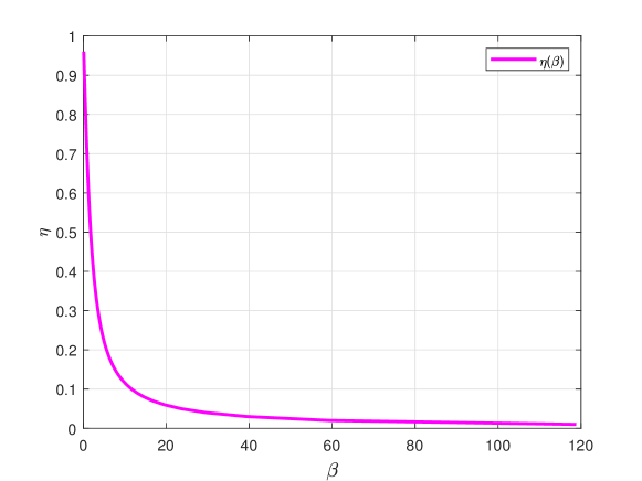
Figure 3: $\eta$ as a decreasing function in $\beta$ for the symmetric case $\alpha=\delta=0.3$.

By the symmetry, it is not hard to see that

$$\mathcal{G}(1)\bigg{|}_{S=1,\sigma=1,\tilde{\pi}=\pi}=\bar{G}(1,\eta,\delta),$$ (97)

where

$$\bar{G}(1,\eta,\delta) :=-\int_{-\infty}^{\infty}\bigg{(}\delta\sqrt{\frac{\eta}{2\pi}}\exp\bigg{[}-\frac{\eta}{2}(u+1)^{2}\bigg{]}+(1-\delta)\sqrt{\frac{\eta}{2\pi}}\exp\bigg{[}-\frac{\eta}{2}(u-1)^{2}\bigg{]}\bigg{)}$$

$$\qquad\times\log\bigg{(}\delta\sqrt{\frac{\eta}{2\pi}}\exp\bigg{[}-\frac{\eta}{2}(u+1)^{2}\bigg{]}+(1-\delta)\sqrt{\frac{\eta}{2\pi}}\exp\bigg{[}-\frac{\eta}{2}(u-1)^{2}\bigg{]}\bigg{)}du$$

$$\qquad+\frac{1}{2\beta}\bigg{[}(\eta-1)\log e-\log\eta\bigg{]}-\frac{1}{2}\log\frac{2\pi}{\eta}-\frac{1}{2}\log e$$

$$\qquad+\frac{1}{2\beta}\log(2\pi)+\frac{1}{2\beta}\log e.$$ (98)

Now, let $\mathcal{C}_{\beta}(\alpha,\delta)$ is the set of all solutions $\eta$ of the equation (90) given $\beta$ and $\alpha$ and $\delta$. Then, by Claim 1 and (63), the free energy can be expressed as

$$\mathcal{F}\bigg{|}_{S=1,\sigma=1,\tilde{\pi}=\pi}=\min_{\eta\in\mathcal{C}_{\beta}(\alpha,\delta)}\bigg{[}\frac{\delta}{\alpha+\delta}\mathcal{G}(-1)+\frac{\alpha}{\alpha+\delta}\mathcal{G}(1)\bigg{]},$$ (99)

where $\mathcal{G}(-1)$ and $\mathcal{G}(1)$ are given in (95) and (97), respectively.

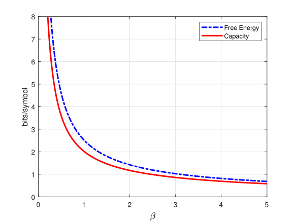
Figure 4: Free energy and average mutual information as functions of $\beta$ for the symmetric case $\alpha=\delta=0.3$.

Solving the optimization problem in (99) is very challenging since $C_{\beta}(\alpha,\delta)$ may have more than one elements, which corresponds to multiple fixed points of the optimization problem in (99). However, by observing that given $\alpha$ and $\delta$, then $\beta$, $\bar{G}(-1,\eta,\alpha)$ and $\bar{G}(1,\eta,\alpha)$ are functions of $\eta$. The multiple fixed-points happen if there exists at least two different values $\eta_{1}$ and $\eta_{2}$ such that $\beta(\eta_{1})=\beta(\eta_{2})$. In simulations, for a fixed $\beta$, we can estimate all the values of $\eta$ such that $|\beta(\eta)-\beta|<10^{-3}$ and then estimate the free energy as a functions of $\eta$ and find the minimum value among them as the free energy corresponding to $\beta(\eta)$. This procedure can avoid the multiple fixed-point problem.

For the symmetric case $\delta=\alpha=0.3$, $\beta$ is a monotone function in $\eta$ (cf. Fig. 3), hence $\mathcal{C}_{\beta}(\alpha,\delta)$ in (99) contains only one element $\eta$, at which we achieve the average mutual information and free energy. For example, in Fig. 4, we plot the free energy and the average mutual information for symmetric case $\delta=\alpha=0.3$.

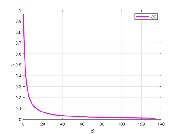
Figure 5: $\eta$ as a decreasing function in $\beta$ for the non-symmetric case $\alpha=0.2$ and $\delta=0.5$.

For the non-symmetric case $\alpha=0.2$ and $\delta=0.5$, $\beta$ is also a monotone function in $\eta$ (cf. Fig. 5), so $\mathcal{C}_{\beta}(\alpha,\delta)$ contains only one element. Then, we obtain the free energy and the average mutual information for this case as in Fig. 6.

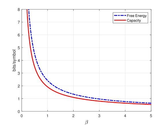
Figure 6: Free energy and average mutual information as functions of $\beta$ for the non-symmetric case $\alpha=0.2$ and $\delta=0.5$.

IV-A2 Markov Chain Monte Carlo (MCMC) vs. Replica Prediction

In this subsection, we use the Markov Chain Monte-Carlo (MCMC) simulation method to estimate the density function $\bm{P}_{\bm{y}|\bm{\Phi}}(\bm{y}|\bm{\Phi})$ and verify our replica predictions in Claims 1 and 2. More specifically, we compare the free energies achieved by the replica prediction and MCMC for the linear model with binary-valued Markov prior defined in (62). Our simulation shows that the free energy curves by the replica method and MCMC nearly coincide to each other for all three cases: (1) i.i.d. prior ($\alpha=\delta=0.5$), (2) symmetric Markov prior $\alpha=\delta=0.3$, (3) asymmetric Markov prior $(\alpha=0.2,\delta=0.5)$ (cf. Figs. 7, 8, and 9). In those simulations, the Metropolis–Hastings algorithm is used where the state $\bm{x}_{t}:=\rm{vec}(\Phi_{t+1},\bm{y}_{t+1})$ and the probability transition $g(\bm{x}_{t+1}|\bm{x}_{t})\sim\mathcal{N}(\bm{x}_{t},\bm{I}_{mn+n})$. Our simulation results show that the replica prediction in Claim 1 for free energy is very closed to MCMC result.

Figure 7: Free energy by Replica Method and MCMC as functions for the i.i.d. prior $\alpha=\delta=0.5$.

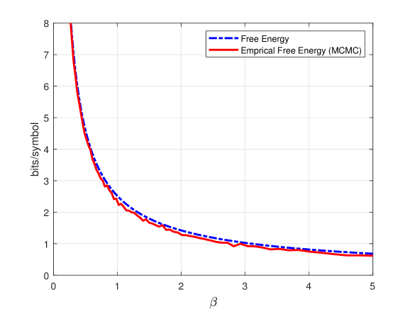
Figure 8: Free energy by Replica Method and MCMC as functions of $\beta$ for the symmetric case $\alpha=\delta=0.3$.

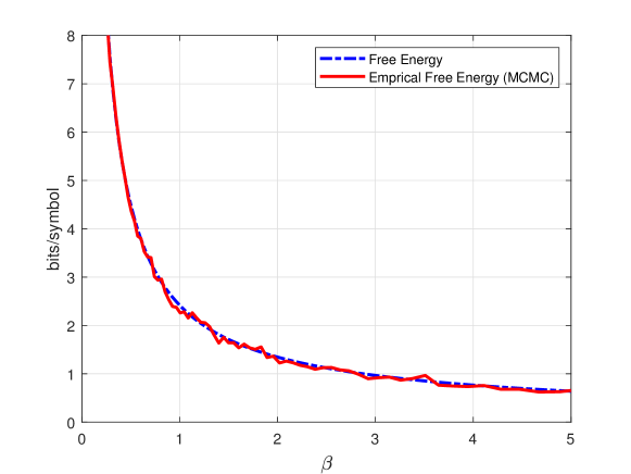
Figure 9: Free energy by Replica Method and MCMC as functions of $\beta$ for the non-symmetric case $\alpha=0.2$ and $\delta=0.5$.

Since MMSE is fixed function of the free energy (or mutual information) [21], these simulation results also indicate that our replica prediction for MMSE in Claim 2 closely approximates the MMSE of the model.

IV-B Gauss-Markov Prior

We consider a Gauss-Markov prior $\{X_{n}\}_{n=1}^{\infty}$ on $\mathcal{X}=\mathbb{R}$, i.e., $X_{n}=\nu X_{n-1}+Z_{n}$, where $Z_{n}\sim\mathcal{N}(0,\sigma_{0}^{2})$ and $\nu\in(0,1)$. Then, the transition probability is

$$\pi(x_{0},x):=\frac{1}{\sigma_{0}\sqrt{2\pi}}\exp\bigg{[}-\frac{1}{2\sigma_{0}^{2}}(x-\nu x_{0})^{2}\bigg{]}.$$ (100)

This means that $X_{n}|X_{n-1}=x_{0}\sim\mathcal{N}(\nu x_{0},\sigma_{0}^{2})$ for all $n\in\mathbb{Z}_{+}$. This is not hard to show that the Markov chain in (100) is irreducible by using [42, Definition 1.1]. We even can show that this Markov chain is a Harris chain by using its definition in [46] or using [42, Theorem 4.2]. To guarantee the irreducible and recurrent properties of this continuous-space Markov chain, we show that $\mathbb{P}[\tau_{A}<\infty|X_{0}=x]=1$ for any $x\in\mathbb{R}$ and $A\in\mathcal{B}(\mathbb{R})$, where $\tau_{A}=\{\inf n\geq 1:X_{n}\in\mathcal{A}\}$.

IV-B1 Free Energy and Average Mutual Information

We assume that all postulated distributions are the same as their true ones for simplicity. Now, given $S=s_{0}\in\mathbb{R}_{+}$, for any $x_{0}\in\mathcal{X}=\mathbb{R}$ and $X_{1}\sim\mathcal{N}(\nu x_{0},\sigma_{0}^{2})$, from (27) and (28), we have

$$\rho_{s} :=\frac{\mathbb{E}[{\sf X}_{1}U|{\sf X}_{0}=x_{0}]-\mathbb{E}[{\sf X}_{1}|{\sf X}_{0}=x_{0}]\mathbb{E}[U|{\sf X}_{0}=x_{0}]}{\sigma_{0}\sqrt{s_{0}\sigma_{0}^{2}+\frac{1}{\eta}}}$$ (101)

$$=\frac{\sqrt{s_{0}}(\nu^{2}x_{0}^{2}+\sigma_{0}^{2})-\nu^{2}x_{0}^{2}\sqrt{s_{0}}}{\sigma_{0}\sqrt{s_{0}\sigma_{0}^{2}+\frac{1}{\eta}}}$$ (102)

$$=\sqrt{\frac{s_{0}\sigma_{0}^{2}}{s_{0}\sigma_{0}^{2}+\frac{1}{\eta}}}.$$ (103)

From (31), (32), and the standard result for MMSE of the bivariate Gaussian distribution (e.g.,[47]), given any $s_{0}\in\mathcal{S}$ and $x_{0}\in\mathcal{X}=\mathbb{R}$, it holds that

$$\mathcal{V}(s_{0};\eta,\eta\mid x_{0}) =\mathcal{E}(s_{0};\eta,\eta\mid x_{0})$$ (104)

$$=\mathbb{E}\bigg{[}\big{(}{\sf X}_{1}-\langle{\sf X}|{\sf X}_{0}=x_{0}\rangle\big{)}^{2}|{\sf X}_{0}=x_{0},s_{0};\eta,\eta\bigg{]}$$ (105)

$$=\operatorname{\mathsf{Var}}({\sf X}_{1}|{\sf X}_{0}=x_{0})(1-\rho_{s}^{2})$$ (106)

$$=\sigma_{0}^{2}\bigg{(}1-\frac{s_{0}\sigma_{0}^{2}}{s\sigma_{0}^{2}+\frac{1}{\eta}}\bigg{)}$$ (107)

$$=\frac{\sigma_{0}^{2}\frac{1}{\eta}}{s_{0}\sigma_{0}^{2}+\frac{1}{\eta}}.$$ (108)

Hence, from (35) and (108), $\eta$ is a solution of the following equation

$$\eta^{-1}=1+\beta\frac{s_{0}\sigma_{0}^{2}}{\eta s_{0}\sigma_{0}^{2}+1}.$$ (109)

In addition, since $\xi=\eta$ and $\sigma=1$, from (33), we have

$$\mathcal{G}(x_{0}) =-\int p_{U|{\sf X}_{0},s_{0};\eta}(u\mid x_{0},s_{0};\eta)\log p_{U|{\sf X}_{0},S;\eta}(u\mid x_{0},S;\eta)du$$

$$\qquad+\frac{1}{2\beta}\bigg{[}(\eta-1)\log e-\log\eta\bigg{]}-\frac{1}{2}\log\frac{2\pi}{\eta}-\frac{1}{2}\log e$$

$$\qquad+\frac{1}{2\beta}\log(2\pi)+\frac{1}{2\beta}\log e$$ (110)

$$=h(U|{\sf X}_{0}=x_{0},S;\eta)$$

$$\qquad+\frac{1}{2\beta}\bigg{[}(\eta-1)\log e-\log\eta\bigg{]}-\frac{1}{2}\log\frac{2\pi}{\eta}-\frac{1}{2}\log e$$

$$\qquad+\frac{1}{2\beta}\log(2\pi)+\frac{1}{2\beta}\log e$$ (111)

$$=\frac{1}{2}\log\bigg{[}2\pi e\bigg{(}s_{0}\sigma_{0}^{2}+\frac{1}{\eta}\bigg{)}\bigg{]}+\frac{1}{2\beta}\bigg{[}(\eta-1)\log e-\log\eta\bigg{]}-\frac{1}{2}\log\frac{2\pi}{\eta}-\frac{1}{2}\log e$$

$$\qquad+\frac{1}{2\beta}\log(2\pi)+\frac{1}{2\beta}\log e.$$ (112)

Since $\mathcal{G}(x_{0})$ does not depend on $x_{0}$, hence we also have a tight bound for this case, and the free energy is equal to

$$\mathcal{F}_{q}\bigg{|}_{\sigma=1,\tilde{\pi}=\pi} =\frac{1}{2}\log\bigg{(}2\pi e\bigg{(}s_{0}\sigma_{0}^{2}+\frac{1}{\eta}\bigg{)}\bigg{)}+\frac{1}{2\beta}\bigg{[}(\eta-1)\log e-\log\eta\bigg{]}$$

$$\qquad-\frac{1}{2}\log\frac{2\pi}{\eta}-\frac{1}{2}\log e+\frac{1}{2\beta}\log(2\pi)+\frac{1}{2\beta}\log e,$$ (113)

where $\eta$ is a solution of (109), which is chosen to minimize $\mathcal{F}_{q}$.

Now, for a fixed $\beta$, (109) is equivalent to

$$s_{0}\sigma_{0}^{2}\eta^{2}+((\beta-1)s_{0}\sigma_{0}^{2}+1)\eta-1=0,$$ (114)

which has solution

$$\eta\in\bigg{\{}\frac{-((\beta-1)s_{0}\sigma_{0}^{2}+1)\pm\sqrt{((\beta-1)s_{0}\sigma_{0}^{2}+1)^{2}+4s_{0}\sigma_{0}^{2}}}{2s_{0}\sigma_{0}^{2}}\bigg{\}}.$$ (115)

Note that $\eta\in(0,1)$ (cf. (109)), it follows that

$$\eta=\frac{-((\beta-1)s_{0}\sigma_{0}^{2}+1)+\sqrt{((\beta-1)s_{0}\sigma_{0}^{2}+1)^{2}+4s_{0}\sigma_{0}^{2}}}{2s_{0}\sigma_{0}^{2}}.$$ (116)

Hence, by (113), the free energy satisfies

$$\mathcal{F}_{q}\bigg{|}_{S=s_{0},\sigma=1,\tilde{\pi}=\pi} =\frac{1}{2}\log\bigg{(}2\pi e\bigg{(}s_{0}\sigma_{0}^{2}+\frac{1}{\eta}\bigg{)}\bigg{)}+\frac{1}{2\beta}\bigg{[}(\eta-1)\log e-\log\eta\bigg{]}$$

$$\qquad-\frac{1}{2}\log\frac{2\pi}{\eta}-\frac{1}{2}\log e+\frac{1}{2\beta}\log(2\pi)+\frac{1}{2\beta}\log e$$ (117)

where

$$\eta=\frac{-((\beta-1)s_{0}\sigma_{0}^{2}+1)+\sqrt{((\beta-1)s_{0}\sigma_{0}^{2}+1)^{2}+4s_{0}\sigma_{0}^{2}}}{2s_{0}\sigma_{0}^{2}}.$$ (118)

IV-B2 Markov Chain Monte Carlo (MCMC) vs. Replica Prediction

In this subsection, we use the same MCMC algorithm as Subsection IV-A2, which is the Metropolis–Hastings algorithm. In the Fig. 10, we plot the free energy curves for the linear model with Markov prior in (100) for three cases $\nu=0.1$, $\nu=0.5$, and $\nu=0.8$. The curves suggest that the free energy does not depend on $\nu$ as we can observe from (117). In these plots, we set $X_{1}\sim\mathcal{N}(0,\frac{\sigma_{0}^{2}}{1-\nu^{2}})$ to force the state distribution of the Markov (Harris) chain $X_{n}\sim\mathcal{N}(0,\frac{\sigma_{0}^{2}}{1-\nu^{2}})$ for all $n\geq 1$. The plot also shows that the replica prediction for the free energy is very closed to the MCMC simulation result. Since the MMSE is a fixed function of the free energy (or mutual information) [21], this also means that the MMSE curve by replica method closely approaches the MMSE of the model.

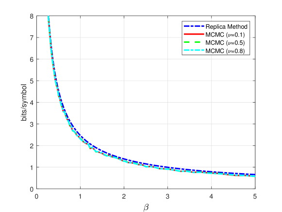
Figure 10: Free energy by replica method and empirical MCMC as functions of $\beta$ for $\sigma_{0}^{2}=1$ and $s_{0}=1$.

IV-C Hidden Markov Prior

In this section, we estimate free energy and mutual information for the linear model in Section II with hidden Markov sources defined in [32, Sect. 7]. The sequence $\{X_{n}\}_{n=1}^{\infty}$ which takes values on $\mathbb{R}$ is generated via

$$p_{X_{n}|\Upsilon_{n}}(x_{n}\mid\upsilon_{n}) =\upsilon_{n}\mathcal{N}(x_{n};0,1)+(1-\upsilon_{n})\delta(x_{n})$$ (119)

$$=\frac{\upsilon_{n}}{\sqrt{2\pi}}\exp\bigg{(}-\frac{x_{n}^{2}}{2}\bigg{)}+(1-\upsilon_{n})\delta(x_{n})$$ (120)

using a time-homogeneous irreducible Markov chain-generated sparsity pattern $\{\Upsilon_{n}\}_{n=1}^{\infty}$ on $\mathcal{S}_{\gamma}=\{0,1\}$. Such a Markov chain is fully described by the following transition stochastic matrix

$$P_{\Upsilon}=\begin{bmatrix}1-\kappa\gamma&\gamma\kappa\\ (1-\kappa)\gamma&1-(1-\kappa)\gamma\end{bmatrix}$$ (121)

for some $\gamma\in(0,1]$ called the Markov independence parameter. This irreducible Markov chain yields a stationary distribution with activity rate $P(\Upsilon_{n}=1)=\kappa$ for all $n\in\mathbb{Z}^{+}$.

IV-C1 Free Energy and Average Mutual Information

First, it is easy to see that the left Perron-Frobenius eigenvector of the stochastic matrix $P_{\Upsilon}$ with unit Manhattan norm is

$$\lambda_{0}=(1-\kappa,\kappa)^{T}.$$ (122)

Observe that

$$P_{{\sf X}_{1},\Upsilon_{1}|{\sf X}_{0},\Upsilon_{0}}(x_{1},\upsilon_{1}\mid x_{0},\upsilon_{0}) =P_{X|\Upsilon}(x_{1}\mid\upsilon_{1})\pi_{\Upsilon}(\upsilon_{0},\upsilon_{1})$$ (123)

where $P_{X|\Upsilon}(\cdot|\cdot)$ is the emission probability of the hidden Markov process.

Hence, the left Perron-Frobenius eigenvector of the stochastic matrix $P_{\pi_{\Upsilon},\mathcal{X}}$ in Subsection III-B has the following form:

$$\lambda^{(\pi_{\Upsilon})}=((1-\kappa)\{l_{0}(x)\}_{x\in\mathcal{X}},\kappa\{l_{1}(x)\}_{x\in\mathcal{X}})^{T},$$ (124)

where $l_{0}:\mathcal{X}\to\mathbb{R}_{+}$ and $l_{1}:\mathcal{X}\to\mathbb{R}_{+}$ and

$$\int_{\mathcal{X}}l_{i}(x)dx=1,\quad\forall i\in\{0,1\}.$$ (125)

By setting $\lambda_{x,0}^{(\pi_{\Upsilon})}:=(1-\kappa)l_{0}(x)$ and $\lambda_{x,1}^{(\pi_{\Upsilon})}=\kappa l_{1}(x)$, it follows that

$$\int_{\mathcal{X}}\lambda_{x,0}^{(\pi_{\Upsilon})}dx =1-\kappa,$$ (126)

$$\int_{\mathcal{X}}\lambda_{x,1}^{(\pi_{\Upsilon})}dx =\kappa.$$ (127)

First, we estimate $\tilde{G}(x_{0},0)$ as a function of $\kappa,\gamma$, and $x_{0}$ for $x_{0}\in\mathcal{X}$. We assume that all postulated distributions are the same as their true ones for simplicity. We also assume that $S=1$ with probability $1$. Now from (49), we have

$$q_{0}(u,x_{0},0,1;\eta) =\mathbb{E}\bigg{[}q_{U|{\sf X}_{0},\Upsilon_{0},{\sf X}_{1},S;\xi}\big{(}u\mid x_{0},0,X,1;\xi\big{)}\bigg{|}S=1\bigg{]}$$ (128)

$$=\mathbb{E}\bigg{[}\sqrt{\frac{\eta}{2\pi}}\exp\bigg{[}-\frac{\eta}{2}(u-{\sf X})^{2}\bigg{]}\bigg{|}{\sf X}_{0}=x_{0},\Upsilon_{0}=0\bigg{]}$$ (129)

$$=\int_{\mathbb{R}}\sum_{\upsilon\in\{0,1\}}\sqrt{\frac{\eta}{2\pi}}\exp\bigg{[}-\frac{\eta}{2}(u-x)^{2}\bigg{]}P_{X_{1}|\Upsilon_{1}}(x|\upsilon)\pi_{\Upsilon}(0,\upsilon)dx$$ (130)

$$=\int_{\mathbb{R}}\sqrt{\frac{\eta}{2\pi}}\exp\bigg{[}-\frac{\eta}{2}(u-x)^{2}\bigg{]}\delta(x)\pi_{\Upsilon}(0,0)dx$$

$$\qquad+\int_{\mathbb{R}}\sqrt{\frac{\eta}{2\pi}}\exp\bigg{[}-\frac{\eta}{2}(u-x)^{2}\bigg{]}\frac{1}{\sqrt{2\pi}}\exp\bigg{(}-\frac{x^{2}}{2}\bigg{)}\pi_{\Upsilon}(0,1)dx$$ (131)

$$=(1-\gamma\kappa)\int_{\mathbb{R}}\sqrt{\frac{\eta}{2\pi}}\exp\bigg{[}-\frac{\eta}{2}(u-x)^{2}\bigg{]}\delta(x)dx$$

$$\qquad+\kappa\gamma\int_{\mathbb{R}}\sqrt{\frac{\eta}{2\pi}}\exp\bigg{[}-\frac{\eta}{2}(u-x)^{2}\bigg{]}\frac{1}{\sqrt{2\pi}}\exp\big{(}-\frac{x^{2}}{2}\bigg{)}dx$$ (132)

$$=(1-\gamma\kappa)\sqrt{\frac{\eta}{2\pi}}\exp\bigg{[}-\frac{\eta u^{2}}{2}\bigg{]}+\kappa\gamma\sqrt{\frac{\eta}{2\pi(1+\eta)}}\exp\bigg{(}-\frac{\eta u^{2}}{2(1+\eta)}\bigg{)},$$ (133)

which does not depend on $x_{0}$.

Similarly, from (50), for all $x_{0}\in\mathcal{X}$, we also have

$$q_{1}(u,x_{0},0,1;\eta) =\mathbb{E}\bigg{[}{\sf X}q_{U|{\sf X}_{0},\Upsilon_{0},{\sf X}_{1},S;\xi}\big{(}u\mid x_{0},0,{\sf X},1;\xi\big{)}\bigg{|}S=1\bigg{]}$$ (134)

$$=\mathbb{E}\bigg{[}{\sf X}\sqrt{\frac{\eta}{2\pi}}\exp\bigg{[}-\frac{\eta}{2}(u-{\sf X})^{2}\bigg{]}\bigg{|}{\sf X}_{0}=x_{0},\Upsilon_{0}=0\bigg{]}$$ (135)

$$=\int_{\mathbb{R}}\sum_{\upsilon\in\{0,1\}}x\sqrt{\frac{\eta}{2\pi}}\exp\bigg{[}-\frac{\eta}{2}(u-x)^{2}\bigg{]}P_{X_{1}|\Upsilon_{1}}(x|\upsilon)\pi_{\Upsilon}(0,\upsilon)dx$$ (136)

$$=\int_{\mathbb{R}}\sqrt{\frac{\eta}{2\pi}}x\exp\bigg{[}-\frac{\eta}{2}(u-x)^{2}\bigg{]}\delta(x)\pi_{\Upsilon}(0,0)dx$$

$$\qquad+\int_{\mathbb{R}}\sqrt{\frac{\eta}{2\pi}}x\exp\bigg{[}-\frac{\eta}{2}(u-x)^{2}\bigg{]}\frac{1}{\sqrt{2\pi}}\exp\bigg{(}-\frac{x^{2}}{2}\bigg{)}\pi_{\Upsilon}(0,1)dx$$ (137)

$$=(1-\gamma\kappa)\int_{\mathbb{R}}\sqrt{\frac{\eta}{2\pi}}x\exp\bigg{[}-\frac{\eta}{2}(u-x)^{2}\bigg{]}\delta(x)dx$$

$$\qquad+\kappa\gamma\int_{\mathbb{R}}\sqrt{\frac{\eta}{2\pi}}x\exp\bigg{[}-\frac{\eta}{2}(u-x)^{2}\bigg{]}\frac{1}{\sqrt{2\pi}}\exp\bigg{(}-\frac{x^{2}}{2}\bigg{)}dx$$ (138)

$$=\kappa\gamma\int_{\mathbb{R}}\sqrt{\frac{\eta}{2\pi}}x\exp\bigg{[}-\frac{\eta}{2}(u-x)^{2}\bigg{]}\frac{1}{\sqrt{2\pi}}\exp\bigg{(}-\frac{x^{2}}{2}\bigg{)}dx$$ (139)

$$=\kappa\gamma\sqrt{\frac{\eta}{2\pi(1+\eta)}}\exp\bigg{(}-\frac{\eta u^{2}}{2(1+\eta)}\bigg{)}\bigg{(}\frac{\eta u}{1+\eta}\bigg{)}.$$ (140)

Therefore, from (47), (48), (133), and (140), we have

$$\langle{\sf X}|x_{0},0\rangle_{q} =\mathbb{E}_{q}\bigg{[}{\sf X}\big{|}{\sf X}_{0}=x_{0},\Upsilon_{0}=0,U,1;\eta\bigg{]}$$ (141)

$$=\frac{q_{1}(U,x_{0},0,1;\eta)}{q_{0}(U,x_{0},0,1;\eta)}$$ (142)

$$=\frac{\kappa\gamma\sqrt{\frac{\eta}{2\pi(1+\eta)}}\exp\bigg{(}-\frac{\eta u^{2}}{2(1+\eta)}\bigg{)}\bigg{(}\frac{\eta u}{1+\eta}\bigg{)}}{(1-\gamma\kappa)\sqrt{\frac{\eta}{2\pi}}\exp\bigg{(}-\frac{\eta u^{2}}{2}\bigg{)}+\kappa\gamma\sqrt{\frac{\eta}{2\pi(1+\eta)}}\exp\bigg{(}-\frac{\eta u^{2}}{2(1+\eta)}\bigg{)}}.$$ (143)

It follows from (51) and (52) that

$$\mathcal{V}(1;\eta,\eta\mid x_{0},0) =\mathcal{E}(1;\eta,\eta\mid x_{0},0)$$ (144)

$$=\mathbb{E}\bigg{[}\big{(}{\sf X}_{1}-\langle{\sf X}|x_{0},0\rangle_{q}\big{)}^{2}|{\sf X}_{0}=x_{0},\Upsilon_{0}=0,1;\eta,\eta\bigg{]}$$ (145)

$$=\mathbb{E}\bigg{[}{\sf X}_{1}^{2}\big{|}{\sf X}_{0}=x_{0},\Upsilon_{0}=0,1;\eta,\eta\bigg{]}-\langle{\sf X}|{\sf X}_{0}=x_{0},\Upsilon_{0}=0\rangle_{q}^{2}$$ (146)

$$=\int_{\mathbb{R}}\sum_{\upsilon\in\{0,1\}}x^{2}P_{X_{1}|\Upsilon_{1}}(x\mid\upsilon)\pi_{\Upsilon}(0,\upsilon)dx$$

$$\qquad-\left(\frac{\kappa\gamma\sqrt{\frac{\eta}{2\pi(1+\eta)}}\exp\bigg{(}-\frac{\eta u^{2}}{2(1+\eta)}\bigg{)}\bigg{(}\frac{\eta u}{1+\eta}\bigg{)}}{(1-\gamma\kappa)\sqrt{\frac{\eta}{2\pi}}\exp\bigg{[}-\frac{\eta u^{2}}{2}\bigg{]}+\kappa\gamma\sqrt{\frac{\eta}{2\pi(1+\eta)}}\exp\bigg{(}-\frac{\eta u^{2}}{2(1+\eta)}\bigg{)}}\right)^{2}$$ (147)

$$=(1-\kappa\gamma)\int_{\mathbb{R}}x^{2}P_{X_{1}|\Upsilon_{1}}(x\mid 0)dx+\kappa\gamma\int_{\mathbb{R}}x^{2}P_{X_{1}|\Upsilon_{1}}(x\mid 1)dx$$

$$\qquad-\left(\frac{\kappa\gamma\sqrt{\frac{\eta}{2\pi(1+\eta)}}\exp\bigg{(}-\frac{\eta u^{2}}{2(1+\eta)}\bigg{)}\bigg{(}\frac{\eta u}{1+\eta}\bigg{)}}{(1-\gamma\kappa)\sqrt{\frac{\eta}{2\pi}}\exp\bigg{[}-\frac{\eta u^{2}}{2}\bigg{]}+\kappa\gamma\sqrt{\frac{\eta}{2\pi(1+\eta)}}\exp\bigg{(}-\frac{\eta u^{2}}{2(1+\eta)}\bigg{)}}\right)^{2}$$ (148)

$$=(1-\kappa\gamma)\int_{\mathbb{R}}x^{2}\delta(x)dx+\kappa\gamma\int_{\mathbb{R}}x^{2}\frac{1}{\sqrt{2\pi}}\exp\bigg{(}-\frac{x^{2}}{2}\bigg{)}dx$$

$$\qquad-\left(\frac{\kappa\gamma\sqrt{\frac{\eta}{2\pi(1+\eta)}}\exp\bigg{(}-\frac{\eta u^{2}}{2(1+\eta)}\bigg{)}\bigg{(}\frac{\eta u}{1+\eta}\bigg{)}}{(1-\gamma\kappa)\sqrt{\frac{\eta}{2\pi}}\exp\bigg{[}-\frac{\eta u^{2}}{2}\bigg{]}+\kappa\gamma\sqrt{\frac{\eta}{2\pi(1+\eta)}}\exp\bigg{(}-\frac{\eta u^{2}}{2(1+\eta)}\bigg{)}}\right)^{2}$$ (149)

$$=\kappa\gamma-\left(\frac{\kappa\gamma\sqrt{\frac{\eta}{2\pi(1+\eta)}}\exp\bigg{(}-\frac{\eta u^{2}}{2(1+\eta)}\bigg{)}\bigg{(}\frac{\eta u}{1+\eta}\bigg{)}}{(1-\gamma\kappa)\sqrt{\frac{\eta}{2\pi}}\exp\bigg{(}-\frac{\eta u^{2}}{2}\bigg{)}+\kappa\gamma\sqrt{\frac{\eta}{2\pi(1+\eta)}}\exp\bigg{(}-\frac{\eta u^{2}}{2(1+\eta)}\bigg{)}}\right)^{2},$$ (150)

which does not depend on $x_{0}$.

Similarly, by symmetry, we also have

$$\mathcal{V}(1;\eta,\eta\mid x_{0},1)=\mathcal{E}(1;\eta,\eta\mid x_{0},1)$$ (151)

$$=1-(1-\kappa)\gamma-\mathbb{E}\left[\left(\frac{(1-(1-\kappa)\gamma)\sqrt{\frac{\eta}{2\pi(1+\eta)}}\exp\bigg{(}-\frac{\eta U^{2}}{2(1+\eta)}\bigg{)}\bigg{(}\frac{\eta U}{1+\eta}\bigg{)}}{(1-\gamma)\kappa\sqrt{\frac{\eta}{2\pi}}\exp\bigg{(}-\frac{\eta U^{2}}{2}\bigg{)}+(1-(1-\kappa)\gamma)\sqrt{\frac{\eta}{2\pi(1+\eta)}}\exp\bigg{(}-\frac{\eta U^{2}}{2(1+\eta)}\bigg{)}}\right)^{2}\right],$$ (152)

which holds for any $x_{0}\in\mathcal{X}$.

Now, by (47), the single-symbol PME for this special case is

$$U={\sf X}_{1}+\frac{1}{\sqrt{\eta}}W.$$ (153)

Observe that

• Under the condition $\Upsilon_{0}=0$, we have

  $$P_{X_{1}}(x) =\sum_{\upsilon\in\{0,1\}}P_{X_{1}|\Upsilon_{1}}(x\mid\upsilon)\pi_{\Upsilon}(0,\upsilon)$$ (154)

  $$=(1-\kappa\gamma)\delta(x)+\frac{\kappa\gamma}{\sqrt{2\pi}}\exp\bigg{(}-\frac{x^{2}}{2}\bigg{)}.$$ (155)

  It follows that:

  $$F_{U}(u) =\mathbb{P}(U\leq u)$$ (156)

  $$=\int_{\mathbb{R}}\mathbb{P}(U\leq u|X_{1}=x)P_{X_{1}}(x)dx$$ (157)

  $$=\int_{\mathbb{R}}\mathbb{P}(W\leq(u-1)\sqrt{\eta})P_{X_{1}}(x)dx$$ (158)

  $$=(1-\kappa\gamma)\int_{\mathbb{R}}\mathbb{P}(W\leq(u-x)\sqrt{\eta})\delta(x)dx+\kappa\gamma\int_{\mathbb{R}}\mathbb{P}(W\leq(u-x)\sqrt{\eta})\frac{1}{\sqrt{2\pi}}\exp\bigg{(}-\frac{x^{2}}{2}\bigg{)}dx$$ (159)

  $$=(1-\kappa\gamma)\int_{\mathbb{R}}\Phi((u-x)\sqrt{\eta})\delta(x)dx+\frac{\kappa\gamma}{2\pi}\int_{-\infty}^{\infty}\int_{-\infty}^{(u-x)\sqrt{\eta}}\exp\bigg{(}-\frac{x^{2}+t^{2}}{2}\bigg{)}dtdx$$ (160)

  $$=(1-\kappa\gamma)\Phi(u\sqrt{\eta})+\frac{\kappa\gamma}{2\pi}\int_{-\infty}^{\infty}\int_{-\infty}^{(u-x)\sqrt{\eta}}\exp\bigg{(}-\frac{x^{2}+t^{2}}{2}\bigg{)}dtdx$$ (161)

  where $\Phi(x):=\frac{1}{\sqrt{2\pi}}\int_{-\infty}^{x}\exp(-t^{2}/2)dt$. From (161), we obtain

  $$f_{U}^{(\rm{HM},1)}(u) =\frac{(1-\gamma\kappa)\sqrt{\eta}}{\sqrt{2\pi}}\exp\bigg{(}-\frac{u^{2}\eta}{2}\bigg{)}+\frac{\kappa\gamma\sqrt{\eta}}{2\pi}\int_{\mathbb{R}}\exp\bigg{(}-\frac{x^{2}+(u-x)^{2}\eta}{2}\bigg{)}dx$$ (162)

  $$=(1-\gamma\kappa)\sqrt{\frac{\eta}{2\pi}}\exp\bigg{(}-\frac{u^{2}\eta}{2}\bigg{)}+\kappa\gamma\sqrt{\frac{\eta}{2\pi(1+\eta)}}\exp\bigg{(}-\frac{u^{2}\eta}{2(1+\eta)}\bigg{)}.$$ (163)

• Similarly, under the condition $\Upsilon_{0}=1$, we have

  $$f_{U}^{(\rm{HM},2)}(u)=(1-\kappa)\gamma\sqrt{\frac{\eta}{2\pi}}\exp\bigg{(}-\frac{u^{2}\eta}{2}\bigg{)}+(1-(1-\kappa)\gamma)\sqrt{\frac{\eta}{2\pi(1+\eta)}}\exp\bigg{(}-\frac{u^{2}\eta}{2(1+\eta)}\bigg{)}.$$ (164)

Hence, from (55), $\eta$ is a solution of the following equation

$$\eta^{-1} =1+\beta\bigg{(}\int_{\mathcal{X}}\lambda_{x,0}^{(\pi_{\Upsilon})}\mathbb{E}[1\mathcal{E}(1;\eta,\eta|x,0)]dx+\int_{\mathcal{X}}\lambda_{x,1}^{(\pi_{\Upsilon})}\mathbb{E}[1\mathcal{E}(1;\eta,\eta|x,1)]dx\bigg{)},$$ (165)

$$=1+\beta\bigg{(}\int_{\mathcal{X}}\lambda_{x,0}^{(\pi_{\Upsilon})}dx\bigg{)}\bigg{(}\gamma\kappa-\mathbb{E}\left[\left(\frac{\kappa\gamma\sqrt{\frac{\eta}{2\pi(1+\eta)}}\exp\bigg{(}-\frac{\eta U^{2}}{2(1+\eta)}\bigg{)}\bigg{(}\frac{\eta U}{1+\eta}\bigg{)}}{(1-\gamma\kappa)\sqrt{\frac{\eta}{2\pi}}\exp\bigg{(}-\frac{\eta U^{2}}{2}\bigg{)}+\kappa\gamma\sqrt{\frac{\eta}{2\pi(1+\eta)}}\exp\bigg{(}-\frac{\eta U^{2}}{2(1+\eta)}\bigg{)}}\right)^{2}\right]\bigg{)}$$

$$\quad+\beta\bigg{(}\int_{\mathcal{X}}\lambda_{x,1}^{(\pi_{\Upsilon})}dx\bigg{)}$$

$$\quad\times\bigg{(}1-(1-\kappa)\gamma-\mathbb{E}\left[\left(\frac{(1-(1-\kappa)\gamma)\sqrt{\frac{\eta}{2\pi(1+\eta)}}\exp\bigg{(}-\frac{\eta U^{2}}{2(1+\eta)}\bigg{)}\bigg{(}\frac{\eta U}{1+\eta}\bigg{)}}{(1-\kappa)\gamma\sqrt{\frac{\eta}{2\pi}}\exp\bigg{(}-\frac{\eta U^{2}}{2}\bigg{)}+(1-(1-\kappa)\gamma)\sqrt{\frac{\eta}{2\pi(1+\eta)}}\exp\bigg{(}-\frac{\eta U^{2}}{2(1+\eta)}\bigg{)}}\right)^{2}\right]\bigg{)}$$ (166)

$$=1+\beta(1-\kappa)\bigg{(}\gamma\kappa-\mathbb{E}\left[\left(\frac{\kappa\gamma\sqrt{\frac{\eta}{2\pi(1+\eta)}}\exp\bigg{(}-\frac{\eta U^{2}}{2(1+\eta)}\bigg{)}\bigg{(}\frac{\eta U}{1+\eta}\bigg{)}}{(1-\gamma\kappa)\sqrt{\frac{\eta}{2\pi}}\exp\bigg{(}-\frac{\eta U^{2}}{2}\bigg{)}+\kappa\gamma\sqrt{\frac{\eta}{2\pi(1+\eta)}}\exp\bigg{(}-\frac{\eta U^{2}}{2(1+\eta)}\bigg{)}}\right)^{2}\right]\bigg{)}$$

$$+\beta\kappa\bigg{(}1-(1-\kappa)\gamma-\mathbb{E}\left[\left(\frac{(1-(1-\kappa)\gamma)\sqrt{\frac{\eta}{2\pi(1+\eta)}}\exp\bigg{(}-\frac{\eta U^{2}}{2(1+\eta)}\bigg{)}\bigg{(}\frac{\eta U}{1+\eta}\bigg{)}}{(1-\kappa)\gamma\sqrt{\frac{\eta}{2\pi}}\exp\bigg{(}-\frac{\eta U^{2}}{2}\bigg{)}+(1-(1-\kappa)\gamma)\sqrt{\frac{\eta}{2\pi(1+\eta)}}\exp\bigg{(}-\frac{\eta U^{2}}{2(1+\eta)}\bigg{)}}\right)^{2}\right]\bigg{)},$$ (167)

where (167) follows from (126) and (127).

Now, since $S=1,\xi=\eta,\sigma=1,\tilde{\pi}_{\Upsilon}=\pi_{\Upsilon}$, from (53), we have

$$\tilde{G}(x_{0},0)\bigg{|}_{\sigma=1,\tilde{\pi}_{\Upsilon}=\pi_{\Upsilon}} =-\int p_{U|X_{0},\Upsilon_{0},S;\eta}(u\mid x_{0},0,1;\eta)\log p_{U|X_{0},\Upsilon_{0},S;\eta}(u\mid x_{0},0,1;\eta)du$$

$$\qquad+\frac{1}{2\beta}\bigg{[}(\eta-1)\log e-\log\eta\bigg{]}-\frac{1}{2}\log\frac{2\pi}{\eta}-\frac{1}{2}\log e$$

$$\qquad+\frac{1}{2\beta}\log(2\pi)+\frac{1}{2\beta}\log e.$$ (168)

On the other hand,

$$p_{U|{\sf X}_{0},\Upsilon_{0},1;\eta}(u\mid x_{0},0,1;\eta) =\int_{\mathbb{R}}p_{U|{\sf X}_{0},\Upsilon_{0},{\sf X}_{1},1;\eta}(u\mid x_{0},0,x,1;\eta)P_{X_{1}|X_{0},\Upsilon_{0}}(x\mid x_{0},0)dx$$ (169)

$$=\int_{\mathbb{R}}\sqrt{\frac{\eta}{2\pi}}\exp\bigg{[}-\frac{\eta}{2}(u-x)^{2}\bigg{]}\bigg{(}\sum_{\upsilon\in\{0,1\}}p_{X_{1}|X_{0},\Upsilon_{0}}(x\mid x_{0},0)\bigg{)}dx$$ (170)

$$=\int_{\mathbb{R}}\sqrt{\frac{\eta}{2\pi}}\exp\bigg{[}-\frac{\eta}{2}(u-x)^{2}\bigg{]}\bigg{(}\sum_{\upsilon\in\{0,1\}}p_{X_{1}|\Upsilon_{1}}(x\mid\upsilon)\pi_{\Upsilon}(0,\upsilon)\bigg{)}dx$$ (171)

$$=(1-\kappa\gamma)\int_{\mathbb{R}}\sqrt{\frac{\eta}{2\pi}}\exp\bigg{[}-\frac{\eta}{2}(u-x)^{2}\bigg{]}\delta(x)dx$$ (172)

$$\qquad+\kappa\gamma\int_{\mathbb{R}}\sqrt{\frac{\eta}{2\pi}}\exp\bigg{[}-\frac{\eta}{2}(u-x)^{2}\bigg{]}\frac{1}{\sqrt{2\pi}}\exp\bigg{(}-\frac{x^{2}}{2}\bigg{)}dx$$ (173)

$$=(1-\kappa\gamma)\sqrt{\frac{\eta}{2\pi}}\exp\bigg{[}-\frac{\eta u^{2}}{2}\bigg{]}+\kappa\gamma\sqrt{\frac{\eta}{2\pi(1+\eta)}}\exp\bigg{[}-\frac{\eta u^{2}}{2(1+\eta)}\bigg{]},$$ (174)

which does not depend on $x_{0}$.

It follows that

$$\tilde{G}(x_{0},0)\bigg{|}_{S=1,\sigma=1,\tilde{\pi}_{\Upsilon}=\pi_{\Upsilon}}=\hat{G}(0,\eta,\kappa,\gamma),\quad\forall x_{0}\in\mathcal{X},$$ (175)

where

$$\hat{G}(0,\eta,\kappa,\gamma) :=-\int_{-\infty}^{\infty}\bigg{(}(1-\kappa\gamma)\sqrt{\frac{\eta}{2\pi}}\exp\bigg{[}-\frac{\eta u^{2}}{2}\bigg{]}+\kappa\gamma\sqrt{\frac{\eta}{2\pi(1+\eta)}}\exp\bigg{[}-\frac{\eta u^{2}}{2(1+\eta)}\bigg{]}\bigg{)}$$

$$\qquad\times\log\bigg{(}(1-\kappa\gamma)\sqrt{\frac{\eta}{2\pi}}\exp\bigg{[}-\frac{\eta u^{2}}{2}\bigg{]}+\kappa\gamma\sqrt{\frac{\eta}{2\pi(1+\eta)}}\exp\bigg{[}-\frac{\eta u^{2}}{2(1+\eta)}\bigg{]}\bigg{)}du$$

$$\qquad+\frac{1}{2\beta}\bigg{[}(\eta-1)\log e-\log\eta\bigg{]}-\frac{1}{2}\log\frac{2\pi}{\eta}-\frac{1}{2}\log e$$

$$\qquad+\frac{1}{2\beta}\log(2\pi)+\frac{1}{2\beta}\log e.$$ (176)

By the symmetry, it is not hard to see that

$$\tilde{G}(x_{0},1)\bigg{|}_{S=1,\sigma=1,\tilde{\pi}_{\Upsilon}=\pi_{\Upsilon}}=\hat{G}(1,\eta,\kappa,\gamma),\quad\forall x_{0}\in\mathcal{X},$$ (177)

where

$$\hat{G}(1,\eta,\kappa,\gamma) :=-\int_{-\infty}^{\infty}\bigg{(}(1-\kappa)\gamma\sqrt{\frac{\eta}{2\pi}}\exp\bigg{[}-\frac{\eta u^{2}}{2}\bigg{]}+(1-(1-\kappa)\gamma)\sqrt{\frac{\eta}{2\pi(1+\eta)}}\exp\bigg{[}-\frac{\eta u^{2}}{2(1+\eta)}\bigg{]}\bigg{)}$$

$$\qquad\times\log\bigg{(}(1-\kappa)\gamma\sqrt{\frac{\eta}{2\pi}}\exp\bigg{(}-\frac{\eta u^{2}}{2}\bigg{)}+(1-(1-\kappa)\gamma)\sqrt{\frac{\eta}{2\pi(1+\eta)}}\exp\bigg{[}-\frac{\eta u^{2}}{2(1+\eta)}\bigg{]}\bigg{)}du$$

$$\qquad+\frac{1}{2\beta}\bigg{[}(\eta-1)\log e-\log\eta\bigg{]}-\frac{1}{2}\log\frac{2\pi}{\eta}-\frac{1}{2}\log e$$

$$\qquad+\frac{1}{2\beta}\log(2\pi)+\frac{1}{2\beta}\log e.$$ (178)

Now, let $\hat{C}_{\beta}(\kappa,\gamma)$ is the set of all solutions $\eta$ of equation (167) given $\beta$ and $\kappa$ and $\gamma$.

From Claim 3 and (126) and (127), we have

$$\mathcal{F}\bigg{|}_{S=1,\sigma=1,\tilde{\pi}_{\Upsilon}=\pi_{\Upsilon}} =\min_{\eta\in\hat{C}_{\beta}(\kappa,\gamma)}\bigg{[}\int_{\mathcal{X}}\lambda_{x,0}^{(\pi_{\Upsilon})}\tilde{G}(x,0)dx+\int_{\mathcal{X}}\lambda_{x,1}^{(\pi_{\Upsilon})}\tilde{G}(x,1)dx\bigg{]}$$ (179)

$$=\min_{\eta\in\hat{C}_{\beta}(\kappa,\gamma)}\bigg{[}(1-\kappa)\hat{G}(0,\eta,\kappa,\gamma)+\kappa\hat{G}(1,\eta,\kappa,\gamma)\bigg{]}.$$ (180)

Figure 11: Free energy and average mutual information as functions of $\beta$ for the symmetric i.i.d. case $\lambda=0.5$ and $\gamma=1$.

Solving the optimization problems in (167) is very challenging. However, by observing that given $\kappa$ and $\gamma$, $\beta$, $\hat{G}(0,\eta,\kappa,\gamma)$ and $\hat{G}(1,\eta,\kappa,\gamma)$ are functions of $\eta$. Hence, we can plot lower and upper bounds for the free energy $\mathcal{F}$ and the average mutual information as functions of $(\kappa,\gamma)$. In Fig. 11, we plot the free energy and the average mutual information for $\kappa=0.5$ and $\gamma=1$, i.e., the sequence $\{X_{n}\}_{n=1}^{\infty}$ is i.i.d. generated.

For the non-symmetric case where $\kappa=0.3$ and $\gamma=0.8$, we obtain the free energy and the average mutual information as in Fig. 12.

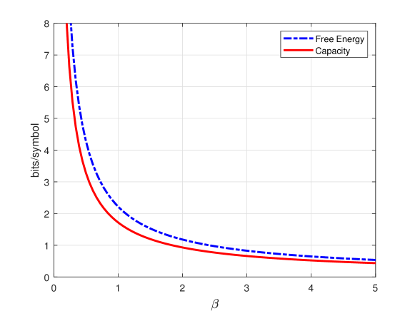
Figure 12: Free energy and average mutual information as functions of $\beta$ for the non-symmetric case $\lambda=0.3$ and $\gamma=0.8$.

IV-C2 Approximate Message Passing Algorithm vs. Replica Prediction

Observe that

$$\mathbb{E}\bigg{[}{\sf X}_{1}^{2}\bigg{|}{\sf X}_{0}=x_{0},\Upsilon_{0}=\upsilon_{0}\bigg{]}$$

$$=\int_{\mathbb{R}}\sum_{\upsilon\in\{0,1\}}x^{2}P_{X_{1},\Upsilon_{1}|X_{0},\Upsilon_{0}}(x,\upsilon\mid x_{0},\upsilon_{0})dx$$ (181)

$$=\sum_{\upsilon\in\{0,1\}}\int_{\mathbb{R}}x^{2}P_{X_{1}|\Upsilon_{1}}(x\mid\upsilon)\pi_{\Upsilon}(\upsilon_{0},\upsilon)dx$$ (182)

$$=\int_{\mathbb{R}}x^{2}\delta(x)\pi_{\Upsilon}(\upsilon_{0},0)dx+\int_{\mathbb{R}}x^{2}\frac{1}{\sqrt{2\pi}}\exp\bigg{(}-\frac{x^{2}}{2}\bigg{)}\pi_{\Upsilon}(\upsilon_{0},1)dx$$ (183)

$$=\pi_{\Upsilon}(\upsilon_{0},1).$$ (184)

Hence, we have

$$\mathbb{E}[{\sf X}_{1}^{2}] =\mathbb{E}\bigg{[}\mathbb{E}\bigg{[}{\sf X}_{1}^{2}\bigg{|}{\sf X}_{0},\Upsilon_{0}\bigg{]}\bigg{]}$$ (185)

$$=\mathbb{E}[\pi_{\Upsilon}(\Upsilon_{0},1)]$$ (186)

$$=P_{\Upsilon}(0)\pi_{\Upsilon}(0,1)+P_{\Upsilon}(1)\pi_{\Upsilon}(1,1)$$ (187)

$$=(1-\kappa)\kappa\gamma+\kappa\big{(}1-(1-\kappa)\gamma\big{)}$$ (188)

$$=\kappa.$$ (189)

On the other hand, given $\Upsilon_{0}=0$, for any $x_{0}\in\mathcal{X}$, we also have

$$\mathbb{E}\big{[}\langle{\sf X}_{1}\big{|}{\sf X}_{0}=x_{0},\Upsilon_{0}=0\rangle^{2}\big{]}=\mathbb{E}\bigg{[}{\sf X}_{1}^{2}\bigg{|}{\sf X}_{0}=x_{0},\Upsilon_{0}=0\bigg{]}-\mathbb{E}\bigg{[}({\sf X}_{1}-\langle{\sf X}_{1}|{\sf X}_{0}=x_{0},\Upsilon_{0}\rangle)^{2}\bigg{|}{\sf X}_{0}=x_{0},\Upsilon_{0}=0\bigg{]}$$ (190)

$$\qquad=\pi_{\Upsilon}(0,1)-\mathbb{E}[\mathcal{E}(1;\eta,\eta\mid x_{0},0)]$$ (191)

$$\qquad=\kappa\gamma-\mathbb{E}[\mathcal{E}(1;\eta,\eta\mid x_{0},0)]$$ (192)

$$\qquad=\mathbb{E}\left[\left(\frac{\kappa\gamma\sqrt{\frac{\eta}{2\pi(1+\eta)}}\exp\bigg{(}-\frac{\eta U^{2}}{2(1+\eta)}\bigg{)}\bigg{(}\frac{\eta U}{1+\eta}\bigg{)}}{(1-\gamma\kappa)\sqrt{\frac{\eta}{2\pi}}\exp\bigg{(}-\frac{\eta U^{2}}{2}\bigg{)}+\kappa\gamma\sqrt{\frac{\eta}{2\pi(1+\eta)}}\exp\bigg{(}-\frac{\eta U^{2}}{2(1+\eta)}\bigg{)}}\right)^{2}\right]:=R_{1}$$ (193)

which does not depend on $x_{0}$, where (193) follows from (150). Here, the expectation in (193) is taken over $U$ with distribution (cf. (163))

$$f_{U}^{(\rm{HM},1)}(u) =\frac{(1-\gamma\kappa)\sqrt{\eta}}{\sqrt{2\pi}}\exp\bigg{(}-\frac{u^{2}\eta}{2}\bigg{)}+\frac{\kappa\gamma\sqrt{\eta}}{2\pi}\int_{\mathbb{R}}\exp\bigg{(}-\frac{x^{2}+(u-x)^{2}\eta}{2}\bigg{)}dx$$ (194)

$$=(1-\gamma\kappa)\sqrt{\frac{\eta}{2\pi}}\exp\bigg{(}-\frac{u^{2}\eta}{2}\bigg{)}+\kappa\gamma\sqrt{\frac{\eta}{2\pi(1+\eta)}}\exp\bigg{(}-\frac{u^{2}\eta}{2(1+\eta)}\bigg{)}.$$ (195)

Similarly, by symmetry, given $\Upsilon_{0}=1$, for any $x_{0}\in\mathcal{X}$, we also have:

$$\mathbb{E}[\langle {\sf X}_{1}|{\sf X}_{0}=1,\Upsilon_{0}=1\rangle^{2}]=\mathbb{E}\bigg{[}{\sf X}_{1}^{2}\bigg{|}{\sf X}_{0}=1,\Upsilon_{0}=1\bigg{]}-\mathbb{E}\bigg{[}({\sf X}_{1}-\langle{\sf X}_{1}|{\sf X}_{0}=1\rangle)^{2}\bigg{|}{\sf X}_{0}=1,\Upsilon_{0}=1\bigg{]}$$ (196)

$$\qquad=1-(1-\kappa)\gamma-\mathbb{E}\bigg{[}\mathcal{E}(1;\eta,\eta\mid 1,1)\bigg{]}$$ (197)

$$\qquad=\mathbb{E}\left[\left(\frac{(1-(1-\kappa)\gamma)\sqrt{\frac{\eta}{2\pi(1+\eta)}}\exp\bigg{(}-\frac{\eta U^{2}}{2(1+\eta)}\bigg{)}\bigg{(}\frac{\eta U}{1+\eta}\bigg{)}}{(1-\kappa)\gamma\sqrt{\frac{\eta}{2\pi}}\exp\bigg{(}-\frac{\eta U^{2}}{2}\bigg{)}+(1-(1-\kappa)\gamma)\sqrt{\frac{\eta}{2\pi(1+\eta)}}\exp\bigg{(}-\frac{\eta U^{2}}{2(1+\eta)}\bigg{)}}\right)^{2}\right]:=R_{2}$$ (198)

which does not depend on $x_{0}$, where the expectation is taken over $U$ with distribution (cf. (164))

$$f_{U}^{(\rm{HM},2)}(u)=(1-\kappa)\gamma\sqrt{\frac{\eta}{2\pi}}\exp\bigg{(}-\frac{u^{2}\eta}{2}\bigg{)}+(1-(1-\kappa)\gamma)\sqrt{\frac{\eta}{2\pi(1+\eta)}}\exp\bigg{(}-\frac{u^{2}\eta}{2(1+\eta)}\bigg{)}.$$ (199)

Hence, from (189), (193), and (198), we obtain from Claim 3 that

$$\rm{MMSE}_{\rm{HM}} :=\lim_{n\to\infty}\frac{1}{n}\mathbb{E}[\|\bm{X}-[\bm{X}]\|_{2}^{2}]$$ (200)

$$=\kappa-\bigg{[}\bigg{(}\int_{\mathcal{X}}\lambda_{x,0}^{(\pi_{\Upsilon})}\bigg{)}R_{1}+\bigg{(}\int_{\mathcal{X}}\lambda_{x,1}^{(\pi_{\Upsilon})}\bigg{)}R_{2}\bigg{]}$$ (201)

$$=\kappa-((1-\kappa)R_{1}+\kappa R_{2}),$$ (202)

where $R_{1}$ and $R_{2}$ are defined in (193) and (198), respectively. Here, (202) follows from (126) and (127).

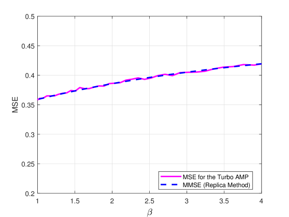
Figure 13: MSE by Turbo AMP algorithm and MMSE by the Replica Method as functions of $\beta$ for the symmetric case $\kappa=0.5,\gamma=1$, i.e., $\{X_{n}\}_{n=1}^{\infty}$ is an i.i.d. sequence.

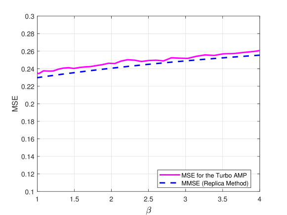
Figure 14: MSE by Turbo AMP algorithm and MMSE by the Replica Method as functions of $\beta$ for the asymmetric case $\kappa=0.3$ and $\gamma=0.8$.

In this section, we compare the MMSE in Claim 3 with the MSE achieved by the AMP algorithm in [32] for $n=1000$ (signal dimension) and $m=\lceil\frac{n}{\beta}\rceil$ (observations). We assume that $S=1$ and $\bm{A}$ is a random matrix where each element is normal distributed $\mathcal{N}(0,1/m)$ as Section II. However, this algorithm assumes some level of sparsity in signal $\bm{X}$. Before introducing the algorithm, we define some new functions:

$$\alpha_{l}(c) =\frac{1}{c+1},$$ (203)

$$\beta_{l}(c) =\bigg{(}\frac{1-\kappa}{\kappa}\bigg{)}\bigg{(}\frac{c+1}{c}\bigg{)},$$ (204)

$$\zeta_{l}(c) =\frac{1}{c(c+1)},$$ (205)

$$F_{l}(\theta;c) =\frac{\alpha_{l}(c)\theta}{1+\beta_{n}(c)e^{-\zeta_{l}(c)|\theta|^{2}}},$$ (206)

$$G_{l}(\theta;c) =\beta_{n}(c)e^{-\zeta_{n}(c)|\theta|^{2}}|F_{n}(\theta;c)|^{2}+\frac{c}{\theta}F_{l}(\theta;c)$$ (207)

$$F_{l}^{\prime}(\theta;c) =\frac{\alpha_{l}(c)}{1+\beta_{l}(c)e^{-\zeta_{l}(c)|\theta|^{2}}}\bigg{[}1+\frac{\zeta_{l}(c)|\theta^{2}|}{1+(\beta_{l}(c)e^{-\zeta_{l}(c)|\theta|^{2}})^{-1}}\bigg{]},\quad\forall l\in\{1,2,\cdots,n\}.$$ (208)

We call this algorithm Turbo AMP since it is based on an approximation of a loopy BP which has demonstrated very accurate results in LDPC and Turbo decoding [32]. The algorithm for our setting is as follows:

1. Initialize

   $$c^{0}=10;\quad\mu_{l}^{0}=0\quad\forall l\in\{1,2,\cdots,n\};\quad z_{k}^{0}=y_{k}\quad\forall k\in\{1,2,\cdots,m\}.$$ (209)

2. Repeat the following for all $i=0,1,2,\cdots$ (we use $10$ iterations in our simulations):

   $$\theta_{l}^{i} =\frac{1}{\sqrt{n}}\sum_{k=1}^{m}A_{kl}z_{k}^{i}+\mu_{l}^{i},\quad\forall l\in\{1,2,\cdots,n\},$$ (210)

   $$\mu_{l}^{i+1} =F_{l}(\theta_{l}^{i};c^{i}),\quad\forall l\in\{1,2,\cdots,n\},$$ (211)

   $$\upsilon_{l}^{i+1} =G_{l}(\theta_{l}^{i};c^{i}),\quad\forall l\in\{1,2,\cdots,n\},$$ (212)

   $$c^{i+1} =1+\frac{\beta}{n}\sum_{l=1}^{n}\upsilon_{l}^{i+1},$$ (213)

   $$z_{k}^{i+1} =y_{k}-\sum_{l=1}^{n}A_{kl}\mu_{l}^{i+1}+\frac{z_{k}^{i}}{m}\sum_{l=1}^{n}F_{l}^{\prime}(\theta_{l}^{i};c^{i}),\quad\forall k\in\{1,2,\cdots,m\}.$$ (214)

Our obtained results are as follows.

• For the symmetric case $\kappa=0.5$ and $\gamma=1$, the Markov model in Section II becomes the linear model with i.i.d. sequence $\{X_{n}\}_{n=1}^{\infty}$ in [4, Sect. II]. Fig. 13 shows that Turbo AMP works well for this case. The gap between the MSE of AMP and the MSE of the Replica Method in Claim 3 is very small.

• For the non-symmetric case $\kappa=0.3$ and $\gamma=0.8$, the Markov model in Section II is very different from the linear model with i.i.d. sequence $\{X_{n}\}_{n=1}^{\infty}$ in [4, Sect. II]. However, Fig. 14 shows that Turbo AMP also works well for this case. The gap between the MSE of Turbo AMP and the upper bound of MSE by using the Replica Method in Claim 3 is also still small. However, the gap is bigger than the symmetric case. The multiple fixed points (multiple solutions) of the equation (167) can be a reason for this gap. Besides, Turbo AMP may not be optimal for this given model although it exploits the Markov structure of the sequence $\{X_{n}\}_{n=1}^{\infty}$ quite well.

V Proofs of main results

This section proves Claims 1–3 using the replica method. We first state some preliminary results which are required to estimate the free energy of the linear model with Markov sources. Then, we obtain the joint moments for the linear model with Markov sources. Finally, we obtain the free energy and joint moments for the linear model with hidden Markov sources based on the results of the linear model with Markov sources.

Lemma 4.

[4, p. 1998] Let $X_{n}^{(a)}$ be replicated vectors with distribution $q_{\bm{X}}$. Define a sequence of $(\nu+1)\times(\nu+1)$ random matrices $\{\bm{Q}_{n}\}_{n=1}^{\infty}$ such that

$$Q_{n}^{(a,b)}=S_{n}X_{n}^{(a)}X_{n}^{(b)}$$ (215)

for all $a,b\in\{0,1,\cdots,\nu\}$ and $n=1,2,\cdots$. Let

$$\bm{T}_{n}=\frac{1}{n}\sum_{k=1}^{n}\bm{Q}_{k},\quad n=1,2,\cdots.$$ (216)

Then, the following holds:

$$\frac{1}{n}\log\mathbb{E}[Z^{\nu}(\bm{Y},\bm{\Phi})]=\frac{1}{n}\log\mathbb{E}\bigg{\{}\exp\bigg{[}m\bigg{(}G^{(\nu)}(\bm{T}_{n})+O(n^{-1})\bigg{)}\bigg{]}\bigg{\}},$$ (217)

where

$$G^{(\nu)}(Q):=-\frac{1}{2}\log\det(I+\Sigma Q)-\frac{1}{2}\log\bigg{(}1+\frac{\nu}{\sigma^{2}}\bigg{)}-\frac{\nu}{2}\log(2\pi\sigma^{2}),$$ (218)

and $\Sigma$ is a $(\nu+1)\times(\nu+1)$ matrix

$$\Sigma=\frac{\beta}{\sigma^{2}+\nu}\begin{bmatrix}\nu&-e^{T}\\ -e&(1+\frac{\nu}{\sigma^{2}})I-\frac{1}{\sigma^{2}}ee^{T}\end{bmatrix},$$ (219)

where $e$ is a $\nu\times 1$ column vector whose entries are all $1$.

The following two lemmas state some new results on large deviations for Markov chains induced by the channel setting. The proofs of these results can be found in Appendix A.

Lemma 5.

Let $\{S_{n}\}_{n=1}^{\infty}$ be an i.i.d. sequence of random variable on a finite set $\mathcal{S}\subset\mathbb{R}^{+}$. Let $\bm{X}:=\{X_{n}\}_{n=1}^{\infty}$ be a Markov chain with states on a Polish space $\mathcal{X}$ with the transition matrix $P=\{\pi(x,x^{\prime})\}_{x,x^{\prime}\in\mathcal{X}}$. Assume this Markov chain is irreducible. Set $\bm{X}^{(0)}=\bm{X}$. Let $\bm{X}^{(a)}:=\{X_{n}^{(a)}\}_{n=1}^{\infty}$ be a set of $\nu$ replica sequences with (postulated) distribution $q_{\bm{X}}$ for each $a=1,2,\cdots,\nu$. This means that

$$p_{\bm{X}^{(0)}\bm{X}^{(1)}\bm{X}^{(2)}\cdots\bm{X}^{(\nu)}}(x^{(0)},x^{(1)},x^{(2)},\cdots,x^{(\nu)})\sim p_{\bm{X}}(x^{(0)})\prod_{i=1}^{\nu}q_{\bm{X}}(x^{(i)}),$$ (220)

where

$$p_{\bm{X}}(x^{(0)}) =\prod_{i=1}^{\infty}\pi(x_{i}^{(0)},x_{i+1}^{(0)})$$ (221)

$$q_{\bm{X}}(x^{(a)}) =\prod_{i=1}^{\infty}\tilde{\pi}(x_{i}^{(a)},x_{i+1}^{(a)}),\qquad\forall a\in[\nu].$$ (222)

Define a new sequence of $(\nu+1)\times(\nu+1)$ random matrices $\{\bm{Q}_{n}\}_{n=1}^{\infty}$ such that

$$Q_{n}^{(a,b)}=S_{n}X_{n}^{(a)}X_{n}^{(b)}$$ (223)

for all $a\in[\nu]$ and $b\in[\nu]$ and for all $n=1,2,\cdots$. Then, $\{\bm{Q}_{n}\}_{n=1}^{\infty}$ is also an irreducible Markov chain with states on $\mathcal{Q}$, where $\mathcal{Q}$ is defined in (3). In addition, the transition probability, namely $P(Q|Q^{\prime})$, of this Markov chain satisfies:

$$P(Q|Q^{\prime})=\frac{\sum_{(s,x_{0},x_{1},\cdots,x_{\nu},s^{\prime},x^{\prime}_{0},x^{\prime}_{1},\cdots,x^{\prime}_{\nu})\in\mathcal{A}_{Q}\times\mathcal{A}_{Q^{\prime}}}P_{S}(s^{\prime})P_{S}(s)p_{X_{n-1}}(x^{\prime}_{0})\pi(x_{0}^{\prime},x_{0})\prod_{i=1}^{\nu}q_{X_{n-1}}(x^{\prime}_{i})\tilde{\pi}(x^{\prime}_{i},x_{i})}{\sum_{(s^{\prime},x^{\prime}_{0},x^{\prime}_{1},\cdots,x^{\prime}_{\nu})\in\mathcal{A}_{Q^{\prime}}}P_{S}(s^{\prime})p_{X_{n-1}}(x^{\prime}_{0})\prod_{i=1}^{\nu}q_{X_{n-1}}(x^{\prime}_{i})},$$ (224)

where $p_{X_{n-1}}(\cdot)$ is the state distribution at time $n-1$ of the Markov chain $\{X_{n}\}_{n=1}^{\infty}$ with the transition probability $\pi$ defined in (6), and $q_{X_{n-1}}(\cdot)$ is the state distribution at time $n-1$ of the Markov chain $\{X_{n}\}_{n=1}^{\infty}$ with the (postulated) transition probability $\tilde{\pi}(\cdot,\cdot)$ defined in (10), and

$$\mathcal{A}_{Q}:=\big{\{}(s,x)\in\mathcal{S}\times\mathcal{X}^{\nu+1}:sxx^{T}=Q\big{\}},\quad\forall Q\in\mathcal{Q}.$$ (225)

Lemma 6.

Let $\mathcal{X}$ be a Polish space with finite cardinality and a irreducible Markov chain $\bm{X}:=\{X_{n}\}_{n=1}^{\infty}$ defined on $\mathcal{X}$ and $\nu$ be a positive integer number. Let $X^{(a)}_{n}$ for $a\in[\nu]$ be replicas of the Markov process $\bm{X}$. Recall the definition of the sequence $\bm{Q}_{n}$ in Lemma 5 and $\bm{T}_{n}=\frac{1}{n}\sum_{j=1}^{n}\bm{Q}_{j}$. Let $P_{n}(U):=\mathbb{P}(\bm{T}_{n}\in U)$ for any measurable set $U$ on the $\sigma$-algebra generated by $\{\bm{Q}_{n}\}_{n=1}^{\infty}$. Then, for and bounded and continuous function $F:\mathcal{Q}\to\mathbb{R}$

$$\lim_{n\to\infty}\frac{1}{n}\log\mathbb{E}\big{[}e^{nF(\bm{T}_{n})}\big{]} =\lim_{n\to\infty}\frac{1}{n}\log\int e^{nF(Q)}dP_{n}(Q)$$ (226)

$$=\sup_{Q}\bigg{[}F(Q)-I(Q)\bigg{]}$$ (227)

where $I(Q)=\sup_{\tilde{Q}}(\mathrm{tr}(\tilde{Q}Q)-\log\rho(P_{\tilde{Q}}))$ and $\rho(P_{\tilde{Q}})$ is the Perron-Frobenius eigenvalue of the matrix $P_{\tilde{Q}}=\{e^{\mathrm{tr}(\tilde{Q}\bar{Q}_{j})}P_{\bar{Q}_{j}|\bar{Q}_{i}}\}_{0\leq i,j\leq M}$ and $M=|\mathcal{Q}|-1$, where $\mathcal{Q}$ and $\{\bar{Q}_{i}\}_{i=0}^{M}$ are defined in Subsection I-D.

Lemma 7.

Recall the definitions of $\{\bar{Q}_{i}\}_{i=0}^{M}$ in Subsection I-D. Recall the definition of the sequence $\bm{Q}_{n}$ in Lemma 5. Then, the following holds:

$$\frac{\partial\log\rho(P_{\tilde{Q}})}{\partial\tilde{Q}}(\tilde{Q})=\frac{1}{\rho(P_{\tilde{Q}})}\sum_{i=0}^{M}\lambda_{i}(\tilde{Q})\sum_{j=0}^{M}\psi_{j}(\tilde{Q})\bar{Q}_{j}P(\bar{Q}_{j}|\bar{Q}_{i})e^{\mathrm{tr}(\tilde{Q}\bar{Q}_{j})},$$ (228)

where $\lambda(\tilde{Q})$ and $\psi(\tilde{Q})$ are left and right eigenvectors associated with the Perron-Frobenius eigenvalue $\rho(P_{\tilde{Q}})$ which are normalized such that $\lambda(\tilde{Q})^{T}\psi(\tilde{Q})=1$.

Proof:

Refer to Appendix B for a detailed proof. ∎

Theorem 8.

Recall the definition of $G^{(\nu)}(Q)$ in Lemma 4. In the large system limit, given any initial state $x_{0}$, the free energy satisfies:

$$\mathcal{F}_{q}\big{|}_{X_{0}=x_{0}}=-\lim_{\nu\to 0}\frac{\partial}{\partial\nu}\sup_{Q}\bigg{[}\beta^{-1}G^{(\nu)}(Q)-I^{(\nu)}(Q)\bigg{]},$$ (229)

where

$$I^{(\nu)}(Q):=\sup_{\tilde{Q}}\bigg{[}\mathrm{tr}(\tilde{Q}Q)-\log\rho(P_{\tilde{Q}})],$$ (230)

and $\rho(P_{\tilde{Q}})$ is the Perron-Frobenius eigenvalue of the matrix $P_{\tilde{Q}}=\{e^{\mathrm{tr}(\tilde{Q}\bar{Q}_{j})}P_{\bar{Q}_{j}|\bar{Q}_{i}}\}_{0\leq i,j\leq M}$ and $M=|\mathcal{Q}|-1$ where $\mathcal{Q}:=\{sxx^{T}\enspace\mbox{for some}\enspace s\in\mathcal{S},\enspace x\in\mathcal{X}^{\nu+1}\}$.

Proof:

The proof follows the same idea as [4, Part A, Sect. IV] with some important changes to account for the Markov setting.

1. By applying Lemma 6, from (217), we obtain

   $$\lim_{n\to\infty}\frac{1}{n}\log\mathbb{E}[Z^{\nu}(\bm{Y},\bm{\Phi})] =\lim_{n\to\infty}\frac{1}{n}\log\mathbb{E}\bigg{\{}\exp\bigg{[}\frac{n}{\beta}\bigg{(}G^{(\nu)}(\bm{T}_{n})+O(n^{-1})\bigg{)}\bigg{]}\bigg{\}}$$ (231)

   $$=\sup_{Q}\bigg{[}\frac{1}{\beta}G^{(\nu)}(Q)-I^{(\nu)}(Q)\bigg{]}.$$ (232)

2. Estimate the free energy.
   

   Now, observe that

   $$\mathcal{F}_{q}\big{|}_{X_{0}=x_{0}} =-\lim_{n\to\infty}\frac{1}{n}\lim_{\nu\to 0}\frac{\partial}{\partial\nu}\log\mathbb{E}[Z^{\nu}(\bm{Y},\bm{\Phi})]$$ (233)

   $$=-\lim_{\nu\to 0}\frac{\partial}{\partial\nu}\lim_{n\to\infty}\frac{1}{n}\log\mathbb{E}[Z^{\nu}(\bm{Y},\bm{\Phi})]$$ (234)

   $$=-\lim_{\nu\to 0}\frac{\partial}{\partial\nu}\sup_{Q}\bigg{[}\frac{1}{\beta}G^{(\nu)}(Q)-I^{(\nu)}(Q)\bigg{]}\bigg{|}_{X_{0}=x_{0}}$$ (235)

   where (233) follows from the assumption (A1), (A2), and the fact (F1), (234) follows from the assumption (A3), and (235) follows from (232).

∎

Theorem 9.

Recall the definitions of $\Sigma$ in Lemma 4, the matrix $P_{\tilde{Q}}$ in Theorem 8, and $\{\bar{Q}_{i}\}_{i=0}^{M}$ in Subsection I-D. The optimal matrix $Q^{*}$ of equation (229) in Theorem 8 must satisfy the following constraints:

$$Q^{*} =\frac{\partial\log\rho(P_{\tilde{Q}^{*}})}{\partial\tilde{Q}^{*}},$$ (236)

$$\tilde{Q}^{*} =-(2\beta)^{-1}(I+\Sigma Q^{*})^{-1}\Sigma,$$ (237)

$$\frac{\partial\log\rho(P_{\tilde{Q}^{*}})}{\partial\tilde{Q}^{*}} =\frac{1}{\rho(P_{\tilde{Q}^{*}})}\sum_{i=0}^{M}\lambda_{i}(\tilde{Q}^{*})\sum_{j=0}^{M}\psi_{j}(\tilde{Q}^{*})\bar{Q}_{j}P(\bar{Q}_{j}|\bar{Q}_{i})e^{\mathrm{tr}(\tilde{Q}^{*}\bar{Q}_{j})},$$ (238)

where $\lambda(\tilde{Q}^{*})$ and $\psi(\tilde{Q}^{*})$ are left and right eigenvectors associated with the Perron-Frobenius eigenvalue $\rho(P_{\tilde{Q}^{*}})$ which are normalized such that $\lambda(\tilde{Q}^{*})^{T}\psi(\tilde{Q}^{*})=1$.

Proof:

Recall the definition of $I^{(\nu)}$ in Theorem 8. It is easy to see that the optimization problem in (232) is equivalent to the following optimization problem:

$$\sup_{Q}\inf_{\tilde{Q}}T^{(\nu)}(Q,\tilde{Q})$$ (239)

where

$$T^{(\nu)}(Q,\tilde{Q}):=-\frac{1}{2\beta}\log\det(I+\Sigma Q)-\mathrm{tr}(\tilde{Q}Q)+\log\rho(P_{\tilde{Q}})-\frac{1}{2\beta}\log\big{(}1+\frac{\nu}{\sigma^{2}}\big{)}-\frac{\nu}{2\beta}\log(2\pi\sigma^{2}).$$ (240)

For an arbitrary $Q$, we first seek critical points with respect to $\tilde{Q}$ and find that for any given $Q$, the extremum in $\tilde{Q}$ satisfies

$$Q=\frac{\partial\log\rho(P_{\tilde{Q}})}{\partial\tilde{Q}}$$ (241)

Let $\tilde{Q}(Q)$ be a solution to (241). We then seek the critical point of $T^{(\nu)}(Q,\tilde{Q}(Q))$ with respect to $Q$.

$$K_{Q,\tilde{Q}}:=\begin{bmatrix}\frac{\partial\tilde{Q}_{0,0}}{\partial Q_{0,0}}&\frac{\partial\tilde{Q}_{0,1}}{\partial Q_{0,1}}&\cdots&\frac{\partial\tilde{Q}_{0,\nu}}{\partial Q_{0,\nu}}\\ \frac{\partial\tilde{Q}_{1,0}}{\partial Q_{1,0}}&\frac{\partial\tilde{Q}_{1,1}}{\partial Q_{1,1}}&\cdots&\frac{\partial\tilde{Q}_{1,\nu}}{\partial Q_{1,\nu}}\\ \vdots&\vdots&\ddots&\vdots\\ \frac{\partial\tilde{Q}_{\nu,0}}{\partial Q_{\nu,0}}&\frac{\partial\tilde{Q}_{\nu,1}}{\partial Q_{\nu,1}}&\cdots&\frac{\partial\tilde{Q}_{\nu,\nu}}{\partial Q_{\nu,\nu}}\end{bmatrix}\in\mathbb{R}^{\nu+1\times\nu+1}.$$ (242)

Observe that

$$\frac{\partial\mathrm{tr}(\tilde{Q}Q)}{\partial Q} =\frac{\partial\mathrm{tr}(Q\tilde{Q})}{\partial Q}$$ (243)

$$=\tilde{Q}+Q\odot K_{Q,\tilde{Q}},$$ (244)

where $\odot$ is the Hadamard product.

It follows that

$$\frac{\partial T^{(\nu)}(Q,\tilde{Q})}{\partial Q} =-\frac{1}{2\beta}(I+\Sigma Q)^{-1}\Sigma-\bigg{(}\tilde{Q}+Q\odot K_{Q,\tilde{Q}}\bigg{)}+\frac{\partial\log\rho(P_{\tilde{Q}})}{\partial Q}$$ (245)

$$=-\frac{1}{2\beta}(I+\Sigma Q)^{-1}\Sigma-\bigg{(}\tilde{Q}+Q\odot K_{Q,\tilde{Q}}\bigg{)}+\frac{\partial\log\rho(P_{\tilde{Q}})}{\partial\tilde{Q}}\odot K_{Q,\tilde{Q}}$$ (246)

$$=-\frac{1}{2\beta}(I+\Sigma Q)^{-1}\Sigma-\tilde{Q}-\bigg{[}Q-\frac{\partial\log\rho(P_{\tilde{Q}})}{\partial\tilde{Q}}\bigg{]}\odot K_{Q,\tilde{Q}}$$ (247)

$$=-\frac{1}{2\beta}(I+\Sigma Q)^{-1}\Sigma-\tilde{Q},$$ (248)

where (245) follows from (244), and (248) follows from (241). Hence, the optimal value of the Theorem 8 is the solution of the following equation systems:

$$Q =\frac{\partial\log\rho(P_{\tilde{Q}})}{\partial\tilde{Q}},$$ (249)

$$\tilde{Q} =-(2\beta)^{-1}(I+\Sigma Q)^{-1}\Sigma.$$ (250)

Finally, from Lemma 7, we also obtain an additional constraint in (238). ∎

Observe that the matrix $\Sigma$ defined in Lemma 4 is invariant if two non-zero indices are interchanged, i.e., $\Sigma$ is symmetric in replicas. Now, we use the RS assumption (A4) to simplify the result in Theorem 8. More specifically, we use the following RS assumption:

Definition 10.

[4, p. 1999] An solution $(\tilde{Q}^{*},Q^{*})$ of the optimization problem in Theorem 8, i.e.,

$$\sup_{Q}\bigg{[}\beta^{-1}G^{(\nu)}(Q)-I^{(\nu)}(Q)\bigg{]}$$

$$=\sup_{Q}\inf_{\tilde{Q}}\bigg{[}-\frac{1}{2\beta}\log\det(I+\Sigma Q)-\mathrm{tr}(\tilde{Q}Q)+\log\rho(P_{\tilde{Q}})-\frac{1}{2\beta}\log\bigg{(}1+\frac{\nu}{\sigma^{2}}\bigg{)}-\frac{\nu}{2\beta}\log(2\pi\sigma^{2})\bigg{]},$$ (251)

is called to satisfy the Replica Symmetry (RS) if both $Q^{*}$ and $\tilde{Q}^{*}$ are invariant under the exchange of any two (nonzero) replica indices. In other words, the extrema can be written as

$$Q^{*} =\begin{bmatrix}r&m&m&\cdots&m\\ m&p&q&\cdots&q\\ m&q&p&\ddots&\vdots\\ \vdots&\vdots&\ddots&\ddots&q\\ m&q&\cdots&q&p\end{bmatrix},$$ (252)

$$\tilde{Q}^{*} =\begin{bmatrix}c&d&d&\cdots&d\\ d&g&f&\cdots&f\\ d&f&g&\ddots&\vdots\\ \vdots&\vdots&\ddots&\ddots&f\\ d&f&\cdots&f&g\end{bmatrix},$$ (253)

where $r,m,p,q,c,d,f,g$ are some real numbers which are not dependent on $\nu$.

Next, we show the following results:

Lemma 11.

Let $\{\bar{Q}_{i}\}_{i=0}^{M}$ be states of the Markov chain $\{\bm{Q}_{n}\}_{n=1}^{\infty}$ in Lemma 5. Assume that

$$\rho(P_{\tilde{Q}^{*}})\to 1\quad\mbox{and}\quad\sum_{j=0}^{M}P(\bar{Q}_{j}|\bar{Q}_{i})e^{\mathrm{tr}(\tilde{Q}^{*}\bar{Q}_{j})}\to 1$$ (254)

for all $i\in[M]$ as $\nu\to 0$. Then, under the RS assumption in Definition 10, the following holds:

$$Q^{*}=\lim_{\nu\to 0}\sum_{i=0}^{M}\lambda_{i}(\tilde{Q}^{*})\mathbb{E}[\bm{Q}_{1}e^{\mathrm{tr}(\tilde{Q}^{*}\bm{Q}_{1})}\big{|}\bm{Q}_{0}=\bar{Q}_{i}]$$ (255)

where $Q^{*}$ is defined in Theorem 9 and $\lambda(\tilde{Q}^{*})$ is a left (positive) eigenvector associated with the Perron-Frobenius eigenvalue $\rho(P_{\tilde{Q}^{*}})$ such that $\|\lambda(\tilde{Q}^{*})\|_{1}=1$. In addition, we have

$$\rho(P_{\tilde{Q}^{*}})=\sum_{i=1}^{M}\lambda_{i}(\tilde{Q}^{*})\mathbb{E}[e^{\rm{tr}(\tilde{Q}^{*}\bm{Q}_{1})}|\bm{Q}_{0}=\bar{Q}_{i}].$$ (256)

Proof:

Since $\psi(\tilde{Q}^{*})$ is the right eigenvector associated with the Perron-Frobenius eigenvalue of the matrix $P_{\tilde{Q}^{*}}$, it holds that

$$\sum_{j=0}^{M}P(\bar{Q}_{j}|\bar{Q}_{i})e^{\mathrm{tr}(\tilde{Q}^{*}\bar{Q}_{j})}\psi_{j}(\tilde{Q}^{*})=\rho(P_{\tilde{Q}^{*}})\psi_{i}(\tilde{Q}^{*})$$ (257)

for all $i\in[M]$. From (257) and (254), we can set $\psi(\tilde{Q}^{*})=(1,1,\cdots,1)^{T}$ is a right eigenvector associated with the eigenvalue $\rho(P_{\tilde{Q}^{*}})$ as $\nu\to 0$.

Hence, from Theorem 9, we have

$$Q^{*}=\lim_{\nu\to 0}\sum_{i=0}^{M}\lambda_{i}(\tilde{Q}^{*})\mathbb{E}[\bm{Q}_{1}e^{\mathrm{tr}(\tilde{Q}^{*}\bm{Q}_{1})}\big{|}\bm{Q}_{0}=\bar{Q}_{i}].$$ (258)

Now, since by Theorem 9, it holds that

$$\sum_{j=0}^{M}\psi_{j}(\tilde{Q}^{*})\lambda_{j}(\tilde{Q}^{*})=1,$$ (259)

so we have

$$\|\lambda(\tilde{Q}^{*})\|_{1}=1.$$ (260)

Now, since $\lambda(\tilde{Q}^{*}):=(\lambda_{0}(\tilde{Q}^{*}),\lambda_{1}(\tilde{Q}^{*}),\cdots,\lambda_{M}(\tilde{Q}^{*}))$ is the left (positive) eigenvector associated with $\rho(P_{\tilde{Q}^{*}})$, it holds that

$$\lambda_{j}(\tilde{Q}^{*})\rho(P_{\tilde{Q}^{*}})=\sum_{i=0}^{M}\lambda_{i}(\tilde{Q}^{*})e^{\rm{tr}(\tilde{Q}^{*}\bar{Q}_{j})}P(\bar{Q}_{j}|\bar{Q}_{i}).$$ (261)

Then, it follows that

$$\rho(P_{\tilde{Q}^{*}}) =\sum_{j=0}^{M}\lambda_{j}(\tilde{Q}^{*})\rho(P_{\tilde{Q}^{*}})$$ (262)

$$=\sum_{j=0}^{M}\sum_{i=1}^{M}\lambda_{i}(\tilde{Q}^{*})e^{\rm{tr}(\tilde{Q}^{*}\bar{Q}_{j})}P(\bar{Q}_{j}|\bar{Q}_{i})$$ (263)

$$=\sum_{i=0}^{M}\lambda_{i}(\tilde{Q}^{*})\sum_{j=0}^{M}e^{\rm{tr}(\tilde{Q}^{*}\bar{Q}_{j})}P(\bar{Q}_{j}|\bar{Q}_{i})$$ (264)

$$=\sum_{i=0}^{M}\lambda_{i}(\tilde{Q}^{*})\mathbb{E}[e^{\rm{tr}(\tilde{Q}^{*}\bm{Q}_{1})}|\bm{Q}_{0}=\bar{Q}_{i}],$$ (265)

where (262) follows from (260), (263) follows from (261). ∎

Lemma 12.

Under the RS assumption in Definition 10, as $\nu\to 0$, the following hold:

$$\rho(P_{\tilde{Q}^{*}})\to 1\quad\mbox{and}\quad\sum_{j=0}^{M}P(\bar{Q}_{j}|\bar{Q}_{i})e^{\mathrm{tr}(\tilde{Q}^{*}\bar{Q}_{j})}\to 1.$$ (266)

Furthermore, it holds that

$$\frac{\partial\log\rho(P_{\tilde{Q}^{*}})}{\partial\nu}\bigg{|}_{\nu=0} =-\frac{\xi}{2}\bigg{(}\mathbb{E}[S]\mathbb{E}_{{\sf X}_{0}\sim\lambda^{(\pi)}}\bigg{[}\mathbb{E}[{\sf X}_{1}^{2}|{\sf X}_{0}]\bigg{]}+\frac{1}{\eta}\bigg{)}\log e+\frac{1}{2}\log\frac{2\pi}{\xi}$$

$$\qquad\qquad+\mathbb{E}_{{\sf X}_{0}\sim\lambda^{(\pi)}}\bigg{[}\mathbb{E}_{S}\bigg{\{}\int_{\mathbb{R}}p_{U|{\sf X}_{0},S;\eta}(u|x_{0},S;\eta)\log q_{U|{\sf X}_{0},S;\eta}(u|x_{0},S;\eta)du\bigg{\}}\bigg{]}.$$ (267)

Proof:

By Lemma 5, $\bm{Q}_{0}-\bm{Q}_{1}-\cdots-\bm{Q}_{n}$ forms a Markov chain on the state-space $\{\bar{Q}_{i}\}_{i=0}^{M}$ defined in Subsection I-D with the following transition matrix:

$$P_{\tilde{Q}}=\left[\begin{array}[]{cccc}P(\bar{Q}_{0}|\bar{Q}_{0})e^{\mathrm{tr}(\tilde{Q}\bar{Q}_{0})}&P(\bar{Q}_{1}|\bar{Q}_{0})e^{\mathrm{tr}(\tilde{Q}\bar{Q}_{1})}&\cdots&P(\bar{Q}_{M}|\bar{Q}_{0})e^{\mathrm{tr}(\tilde{Q}\bar{Q}_{M})}\\ P(\bar{Q}_{0}|\bar{Q}_{1})e^{\mathrm{tr}(\tilde{Q}\bar{Q}_{0})}&P(\bar{Q}_{1}|\bar{Q}_{1})e^{\mathrm{tr}(\tilde{Q}\bar{Q}_{1})}&\cdots&P(\bar{Q}_{M}|\bar{Q}_{1})e^{\mathrm{tr}(\tilde{Q}\bar{Q}_{M})}\\ \vdots&\vdots&\vdots&\vdots\\ P(\bar{Q}_{0}|\bar{Q}_{M})e^{\mathrm{tr}(\tilde{Q}\bar{Q}_{0})}&P(\bar{Q}_{1}|\bar{Q}_{M})e^{\mathrm{tr}(\tilde{Q}\bar{Q}_{1})}&\cdots&P(\bar{Q}_{M}|\bar{Q}_{M})e^{\mathrm{tr}(\tilde{Q}\bar{Q}_{M})}\end{array}\right].$$ (272)

where

$$P(\bar{Q}_{j}|\bar{Q}_{i}):=\mathbb{P}(\bm{Q}_{1}=\bar{Q}_{j}|\bm{Q}_{0}=\bar{Q}_{i})$$ (273)

and $\bm{Q}_{0}$ and $\bm{Q}_{1}$ are random (state) matrices at time $0$ and $1$, respectively.

By [41], we have

$$\min_{i\in[M]}\sum_{j=0}^{M}P(\bm{Q}_{1}=\bar{Q}_{j}|\bm{Q}_{0}=\bar{Q}_{i})e^{\mathrm{tr}(\tilde{Q}^{*}\bar{Q}_{j})}\leq\rho(P_{\tilde{Q}^{*}})\leq\max_{i\in[M]}\sum_{j=0}^{M}P(\bm{Q}_{1}=\bar{Q}_{j}|\bm{Q}_{0}=\bar{Q}_{i})e^{\mathrm{tr}(\tilde{Q}^{*}\bar{Q}_{j})}.$$ (274)

It follows that

$$\min_{i\in[M]}\mathbb{E}\bigg{[}e^{\mathrm{tr}(\tilde{Q}^{*}\bm{Q}_{1})}|\bm{Q}_{0}=\bar{Q}_{i}\bigg{]}\leq\rho(P_{\tilde{Q}^{*}})\leq\max_{i\in[M]}\mathbb{E}\bigg{[}e^{\mathrm{tr}(\tilde{Q}^{*}\bm{Q}_{1})}|\bm{Q}_{0}=\bar{Q}_{i}\bigg{]}.$$ (275)

First, we show that

$$\lim_{\nu\to 0}\rho(P_{\tilde{Q}^{*}})=1.$$ (276)

To show (276), it is enough to show that

$$\mathbb{E}\bigg{[}e^{\mathrm{tr}(\tilde{Q}^{*}\bm{Q}_{1})}\big{|}\bm{Q}_{0}=\bar{Q}_{i}\bigg{]}\to 1$$ (277)

for all $i\in[M]$. Indeed, by the definition of $\{\bm{Q}_{n}\}_{n=1}^{\infty}$ in Lemma 5, we have $\bm{Q}_{1}=S_{1}\bm{X}_{1}\bm{X}_{1}^{T}$. Hence, we have

$$\mathbb{E}\bigg{[}e^{\mathrm{tr}(\tilde{Q}^{*}\bm{Q}_{1})}\big{|}\bm{Q}_{0}=\bar{Q}_{i}\bigg{]}=\mathbb{E}\bigg{[}e^{S_{1}\bm{X}_{1}\tilde{Q}^{*}\bm{X}_{1}^{T}}\bigg{|}\bm{Q}_{0}=\bar{Q}_{i}\bigg{]}$$ (278)

$$=\mathbb{E}\bigg{[}e^{S_{1}\bm{X}_{1}\tilde{Q}^{*}\bm{X}_{1}^{T}}\bigg{|}\bm{Q}_{0}=\bar{Q}_{i}\bigg{]}$$ (279)

$$=\mathbb{E}\bigg{[}\exp\bigg{(}S_{1}\bigg{[}2d\sum_{a=1}^{\nu}X_{1}^{(0)}X_{1}^{(a)}+2f\sum_{1\leq a<b\leq\nu}X_{1}^{(a)}X_{1}^{(b)}+c\big{(}X_{1}^{(0)}\big{)}^{2}+g\sum_{a=1}^{\nu}\big{(}X_{1}^{(a)}\big{)}^{2}\bigg{]}\bigg{)}\bigg{|}\bm{Q}_{0}=\bar{Q}_{i}\bigg{]},$$ (280)

where (280) follows from RS assumption in Definition 10.

Now, the eight parameters $(r,m,p,q,f,g)$ that define $Q^{*}$ and $\tilde{Q}^{*}$ are the solution to the joint equations (236) and (237) in Theorem 9. Using (237), it can be shown that [4, Eq. (123)]

$$c =0,$$ (281)

$$d =\frac{1}{2[\sigma^{2}+\beta(p-q)]},$$ (282)

$$f =\frac{1+\beta(r-2m+q)}{2[\sigma^{2}+\beta(p-q)]^{2}},$$ (283)

$$g =f-d.$$ (284)

Now, define

$$\eta=\frac{2d^{2}}{f},\quad\xi=2d.$$ (285)

In addition, for the simplicity of presentation, let $S:=S_{1}$. Then, by using some algebraic calculation and using the following interesting identity

$$e^{x^{2}}=\sqrt{\frac{\eta}{2\pi}}\int\exp\bigg{[}-\frac{\eta}{2}u^{2}+\sqrt{2\eta}xu\bigg{]}du,\quad\forall x,\eta,$$ (286)

from (280), we have (cf. a similar formula in [4, Eq. (125)]):

$$\mathbb{E}\bigg{[}e^{\mathrm{tr}(\tilde{Q}^{*}\bm{Q}_{1})}\big{|}\bm{Q}_{0}=\bar{Q}_{i}\bigg{]}$$ (287)

$$\qquad=\mathbb{E}\bigg{[}\sqrt{\frac{\eta}{2\pi}}\int\exp\bigg{[}-\frac{\eta}{2}(u-\sqrt{S}X_{1})^{2}\bigg{]}$$

$$\qquad\qquad\times\bigg{[}\mathbb{E}_{q}\bigg{\{}\exp\bigg{[}-\frac{\xi}{2}u^{2}-\frac{\xi}{2}\big{(}u-\sqrt{S}X\big{)}^{2}\bigg{]}\bigg{|}\bm{Q}_{0}=\bar{Q}_{i}\bigg{\}}\bigg{]}^{\nu}du\bigg{|}\bm{Q}_{0}=\bar{Q}_{i}\bigg{]}$$ (288)

$$\qquad\to\mathbb{E}\bigg{[}\sqrt{\frac{\eta}{2\pi}}\int\exp\bigg{[}-\frac{\eta}{2}(u-\sqrt{S}X_{1})^{2}\bigg{]}du\bigg{|}\bm{Q}_{0}=\bar{Q}_{i}\bigg{]}$$ (289)

$$\qquad=\mathbb{E}\big{[}1\big{|}\bm{Q}_{0}=\bar{Q}_{i}\big{]}$$ (290)

$$\qquad=1,$$ (291)

where (289) follows from the dominated convergence theorem [43]. Here, as above, we note that the conditional event $\{\bm{Q}_{0}=\bar{Q}_{i}\}$ only affects the distributions of $S$, ${\sf X}$, and ${\sf X}_{1}$.

Next, we prove that

$$\lim_{\nu\to 0}\frac{\partial\rho(\tilde{Q}^{*})}{\partial\nu} =\bigg{(}\frac{1}{\log e}\bigg{)}\bigg{(}-\frac{\xi}{2}\bigg{(}\mathbb{E}[S]\mathbb{E}_{{\sf X}_{0}\sim\lambda^{(\pi)}}\bigg{[}\mathbb{E}[{\sf X}_{1}^{2}|{\sf X}_{0}]\bigg{]}+\frac{1}{\eta}\bigg{)}\log e+\frac{1}{2}\log\frac{2\pi}{\xi}$$

$$\qquad\qquad+\mathbb{E}_{{\sf X}_{0}\sim\lambda^{(\pi)}}\bigg{[}\mathbb{E}_{S}\bigg{\{}\int_{\mathbb{R}}p_{U|{\sf X}_{0},S;\eta}(u|x_{0},S;\eta)\log q_{U|{\sf X}_{0},S;\eta}(u|x_{0},S;\eta)du\bigg{\}}\bigg{]}\bigg{)}.$$ (292)

Indeed, at $\nu=0$, it holds from (288) that

$$\min_{i\in[M]}\mathbb{E}\bigg{[}e^{\mathrm{tr}(\tilde{Q}^{*}\bm{Q}_{1})}|\bm{Q}_{0}=\bar{Q}_{i}\bigg{]}\bigg{|}_{\nu=0}=1=\max_{i\in[M]}\mathbb{E}\bigg{[}e^{\mathrm{tr}(\tilde{Q}^{*}\bm{Q}_{1})}|\bm{Q}_{0}=\bar{Q}_{i}\bigg{]}\bigg{|}_{\nu=0}.$$ (293)

Therefore, from (275) and (293), it holds that

$$\rho(P_{\tilde{Q}^{*}})\big{|}_{\nu=0}=1.$$ (294)

On the other hand, observe that

$$\mathbb{E}\bigg{[}e^{\mathrm{tr}(\tilde{Q}^{*}\bm{Q}_{1})}\bigg{|}\bm{Q}_{0}=\bar{Q}_{i}\bigg{]} =\mathbb{E}\bigg{[}e^{S\bm{X}_{1}\tilde{Q}^{*}\bm{X}_{1}^{T}}\bigg{|}\bm{Q}_{0}=\bar{Q}_{i}\bigg{]}$$ (295)

$$=\mathbb{E}\bigg{\{}\sqrt{\frac{\eta}{2\pi}}\int_{\mathbb{R}}\exp\bigg{[}-\frac{\eta}{2}\big{(}u-\sqrt{S}{\sf X}_{1}\big{)}^{2}\bigg{]}$$

$$\qquad\qquad\times\bigg{[}\mathbb{E}_{q}\bigg{\{}\exp\bigg{[}-\frac{\xi}{2}u^{2}-\frac{\xi}{2}(u-\sqrt{S}{\sf X})^{2}\bigg{]}\bigg{|}S\bigg{\}}\bigg{]}^{\nu}du\bigg{|}\bm{Q}_{0}=\bar{Q}_{i}\bigg{\}}$$ (296)

where (295) follows from (278), (296) follows by using (281)–(285) (see [4, Eq. (125)]). Hence, we have

$$\frac{\partial}{\partial\nu}\mathbb{E}\bigg{[}e^{\mathrm{tr}(\tilde{Q}^{*}\bm{Q}_{1})}\bigg{|}\bm{Q}_{0}=\bar{Q}_{i}\bigg{]}$$

$$\qquad=\bigg{(}\frac{1}{\log e}\bigg{)}\mathbb{E}\bigg{\{}\sqrt{\frac{\eta}{2\pi}}\int_{\mathbb{R}}\exp\bigg{[}-\frac{\eta}{2}\big{(}u-\sqrt{S}{\sf X}_{1}\big{)}^{2}\bigg{]}$$

$$\qquad\qquad\times\bigg{[}\mathbb{E}_{q}\bigg{\{}\exp\bigg{[}-\frac{\xi}{2}u^{2}-\frac{\xi}{2}(u-\sqrt{S}{\sf X})^{2}\bigg{]}\bigg{|}S\bigg{\}}\bigg{]}^{\nu}$$

$$\qquad\qquad\qquad\times\log\bigg{(}\mathbb{E}_{q}\bigg{\{}\exp\bigg{[}-\frac{\xi}{2}u^{2}-\frac{\xi}{2}(u-\sqrt{S}{\sf X})^{2}\bigg{]}\bigg{|}S\bigg{\}}\bigg{)}du\bigg{|}\bm{Q}_{0}=\bar{Q}_{i}\bigg{\}}$$ (297)

Hence, given ${\sf X}_{0}=x_{0}$ and $S_{0}=s_{0}$, it holds from (296) that

$$\lim_{\nu\to 0}\frac{\partial}{\partial\nu}\mathbb{E}\bigg{[}e^{\mathrm{tr}(\tilde{Q}^{*}\bm{Q}_{1})}\bigg{|}\bm{Q}_{0}=\bar{Q}_{i}\bigg{]}$$

$$\qquad=\lim_{\nu\to 0}\bigg{(}\frac{1}{\log e}\bigg{)}\mathbb{E}\bigg{\{}\sqrt{\frac{\eta}{2\pi}}\int_{\mathbb{R}}\exp\bigg{[}-\frac{\eta}{2}\big{(}u-\sqrt{S}{\sf X}_{1}\big{)}^{2}\bigg{]}$$

$$\qquad\qquad\times\bigg{[}\mathbb{E}_{q}\bigg{\{}\exp\bigg{[}-\frac{\xi}{2}u^{2}-\frac{\xi}{2}(u-\sqrt{S}{\sf X})^{2}\bigg{]}\bigg{|}S\bigg{\}}\bigg{]}^{\nu}$$

$$\qquad\qquad\qquad\times\log\bigg{(}\mathbb{E}_{q}\bigg{\{}\exp\bigg{[}-\frac{\xi}{2}u^{2}-\frac{\xi}{2}(u-\sqrt{S}{\sf X})^{2}\bigg{]}\bigg{|}S\bigg{\}}\bigg{)}du\bigg{|}\bm{Q}_{0}=\bar{Q}_{i}\bigg{\}}$$ (298)

$$\qquad=\bigg{(}\frac{1}{\log e}\bigg{)}\mathbb{E}\bigg{\{}\sqrt{\frac{\eta}{2\pi}}\int_{\mathbb{R}}\exp\bigg{[}-\frac{\eta}{2}\big{(}u-\sqrt{S}{\sf X}_{1}\big{)}^{2}\bigg{]}$$

$$\qquad\qquad\times\log\bigg{(}\mathbb{E}_{q}\bigg{\{}\exp\bigg{[}-\frac{\xi}{2}u^{2}-\frac{\xi}{2}(u-\sqrt{S}{\sf X})^{2}\bigg{]}\bigg{|}S\bigg{\}}\bigg{)}du\bigg{|}{\sf X}_{0}=x_{0}\bigg{\}}$$ (299)

$$\qquad=\bigg{(}\frac{1}{\log e}\bigg{)}\bigg{(}-\frac{\xi}{2}\mathbb{E}\bigg{\{}\sqrt{\frac{\eta}{2\pi}}\int_{\mathbb{R}}\exp\bigg{[}-\frac{\eta}{2}\big{(}u-\sqrt{S}{\sf X}_{1}\big{)}^{2}\bigg{]}u^{2}du\bigg{|}{\sf X}_{0}=x_{0}\bigg{\}}$$

$$\qquad\qquad+\mathbb{E}\bigg{\{}\int_{\mathbb{R}}p_{U|{\sf X}_{0},{\sf X}_{1},S;\eta}(u|{\sf X}_{0},{\sf X}_{1},S;\eta)$$

$$\qquad\qquad\times\log\bigg{(}\mathbb{E}_{q}\bigg{\{}\sqrt{\frac{2\pi}{\xi}}q_{U|{\sf X}_{0},{\sf X}_{1},S;\eta}(u|{\sf X}_{0},{\sf X}_{1},S;\eta)\bigg{|}S\bigg{\}}\bigg{)}du\bigg{|}{\sf X}_{0}=x_{0}\bigg{\}}\bigg{)}$$ (300)

$$\qquad=\bigg{(}\frac{1}{\log e}\bigg{)}\bigg{(}-\frac{\xi}{2}\bigg{(}\mathbb{E}[S]\mathbb{E}[{\sf X}_{1}^{2}|{\sf X}_{0}=x_{0}]+\frac{1}{\eta}\bigg{)}\log e+\frac{1}{2}\log\frac{2\pi}{\xi}$$ (301)

$$\qquad\qquad+\mathbb{E}_{S}\bigg{\{}\int_{\mathbb{R}}\mathbb{E}_{\pi(x_{0},\cdot)}\bigg{[}p_{U|{\sf X}_{0},{\sf X}_{1},S;\eta}(u|x_{0},{\sf X}_{1},S;\eta)\bigg{|}S\bigg{]}$$

$$\qquad\qquad\times\log\bigg{(}\mathbb{E}_{\tilde{\pi}(x_{0},\cdot)}\bigg{[}q_{U|{\sf X}_{0},{\sf X}_{1},S;\eta}(u|x_{0},{\sf X}_{1},S;\eta)\bigg{|}S\bigg{]}\bigg{)}du\bigg{|}{\sf X}_{0}=x_{0}\bigg{\}}\bigg{)}$$ (302)

$$\qquad=\bigg{(}\frac{1}{\log e}\bigg{)}\bigg{(}-\frac{\xi}{2}\bigg{(}\mathbb{E}[S{\sf X}_{1}^{2}|{\sf X}_{0}=x_{0}]+\frac{1}{\eta}\bigg{)}\log e+\frac{1}{2}\log\frac{2\pi}{\xi}$$ (303)

$$\qquad\qquad+\mathbb{E}_{S}\bigg{\{}\int_{\mathbb{R}}\mathbb{E}_{\pi(x_{0},\cdot)}\big{[}p_{U|{\sf X}_{0},{\sf X}_{1},S;\eta}(u|{\sf X}_{0},{\sf X}_{1},S;\eta)\big{]}$$

$$\qquad\qquad\times\log\bigg{(}\mathbb{E}_{\tilde{\pi}(x_{0},\cdot)}\bigg{\{}q_{U|{\sf X}_{0},{\sf X}_{1},S;\eta}(u|{\sf X}_{0},{\sf X}_{1},S;\eta)\bigg{|}S\bigg{\}}\bigg{)}du\bigg{|}{\sf X}_{0}=x_{0}\bigg{\}}\bigg{)}$$ (304)

$$\qquad=\bigg{(}\frac{1}{\log e}\bigg{)}\bigg{(}-\frac{\xi}{2}\bigg{(}\mathbb{E}[S]\mathbb{E}[{\sf X}_{1}^{2}|{\sf X}_{0}=x_{0}]+\frac{1}{\eta}\bigg{)}\log e+\frac{1}{2}\log\frac{2\pi}{\xi}$$

$$\qquad\qquad+\mathbb{E}_{S}\bigg{\{}\int_{\mathbb{R}}p_{U|{\sf X}_{0},S;\eta}(u|x_{0},S;\eta)\log q_{U|{\sf X}_{0},S;\eta}(u|x_{0},S;\eta)du\bigg{\}}\bigg{)},$$ (305)

which is a constant which does not depend on $\bar{Q}_{i}$, where (299) follows from the dominated convergence theorem [43]. Here, we note that the conditional event $\{\bm{Q}_{0}=\bar{Q}_{i}\}$ only affects the distribution of ${\sf X}$ and ${\sf X}_{1}$.

Now, from Lemma 11, it holds that

$$\frac{\partial\rho(P_{\tilde{Q}^{*}})}{\partial\nu}\bigg{|}_{\nu=0} =\lim_{\nu\to 0}\frac{\rho(P_{\tilde{Q}^{*}})\big{|}_{\nu}-1}{\nu}$$ (306)

$$=\lim_{\nu\to 0}\sum_{i=1}^{M}\lambda_{i}(\tilde{Q}^{*})\bigg{(}\frac{\mathbb{E}[e^{\rm{tr}(\tilde{Q}^{*}\bm{Q}_{1})}|\bm{Q}_{0}=\bar{Q}_{i}]-1\big{)}}{\nu}\bigg{)}$$ (307)

where (306) follows from (294).

Finally, as $\nu\to 0$, it holds that $\tilde{Q}^{*}\to c=0$ by (281) and (253) of Definition 10. Therefore, we have $P_{\tilde{Q}^{*}}\to P_{S}\otimes P_{\pi}$ and $M\to\big{|}\{sx^{2}:(x,s)\in\mathcal{X}\times\mathcal{S}\}\big{|}:=M_{0}$, where $\otimes$ is denoted as the Kronecker product. It follows that for each fixed $S=s$, $\lambda(\tilde{Q})\to\tilde{\lambda}^{(\pi)}$ where $\tilde{\lambda}^{(\pi)}$ is the left Perron-Frobenius eigenvector of the stochastic matrix $P_{S}\otimes P_{\pi}$ such that $\|\lambda^{(\pi)}\|_{1}=1$. By Lemma 37, the left Perron-Frobenius eigenvector exists, and it is unique up to a positive scaling factor, so $\tilde{\lambda}^{(\pi)}$ exists uniquely.

Let $\lambda^{(\pi)}$ be the marginal distribution of $\tilde{\lambda}^{(\pi)}$. Then, from (305) and (307), we obtain

$$\frac{\partial\rho(P_{\tilde{Q}^{*}})}{\partial\nu}\bigg{|}_{\nu=0} =\sum_{s\in\mathcal{S}}\sum_{x_{0}\in\mathcal{X}_{0}}\tilde{\lambda}^{(\pi)}_{s,x_{0}}\bigg{(}\frac{1}{\log e}\bigg{)}\bigg{(}-\frac{\xi}{2}\bigg{(}\mathbb{E}[S]\mathbb{E}[{\sf X}_{1}^{2}|{\sf X}_{0}=x_{0}]+\frac{1}{\eta}\bigg{)}\log e+\frac{1}{2}\log\frac{2\pi}{\xi}$$

$$\qquad\qquad+\mathbb{E}_{S}\bigg{\{}\int_{\mathbb{R}}p_{U|{\sf X}_{0},S;\eta}(u|x_{0},S;\eta)\log q_{U|{\sf X}_{0},S;\eta}(u|x_{0},S;\eta)du\bigg{\}}\bigg{)}$$ (308)

$$=\sum_{x_{0}\in\mathcal{X}_{0}}\lambda^{(\pi)}_{x_{0}}\bigg{(}\frac{1}{\log e}\bigg{)}\bigg{(}-\frac{\xi}{2}\bigg{(}\mathbb{E}[S]\mathbb{E}[{\sf X}_{1}^{2}|{\sf X}_{0}=x_{0}]+\frac{1}{\eta}\bigg{)}\log e+\frac{1}{2}\log\frac{2\pi}{\xi}$$

$$\qquad\qquad+\mathbb{E}_{S}\bigg{\{}\int_{\mathbb{R}}p_{U|{\sf X}_{0},S;\eta}(u|x_{0},S;\eta)\log q_{U|{\sf X}_{0},S;\eta}(u|x_{0},S;\eta)du\bigg{\}}\bigg{)}$$ (309)

$$=\bigg{(}\frac{1}{\log e}\bigg{)}\bigg{(}-\frac{\xi}{2}\bigg{(}\mathbb{E}[S]\mathbb{E}_{{\sf X}_{0}\sim\lambda^{(\pi)}}\bigg{[}\mathbb{E}[{\sf X}_{1}^{2}|{\sf X}_{0}]\bigg{]}+\frac{1}{\eta}\bigg{)}\log e+\frac{1}{2}\log\frac{2\pi}{\xi}$$

$$\qquad\qquad+\mathbb{E}_{{\sf X}_{0}\sim\lambda^{(\pi)}}\bigg{[}\mathbb{E}_{S}\bigg{\{}\int_{\mathbb{R}}p_{U|{\sf X}_{0},S;\eta}(u|x_{0},S;\eta)\log q_{U|{\sf X}_{0},S;\eta}(u|x_{0},S;\eta)du\bigg{\}}\bigg{]}\bigg{)}.$$ (310)

This concludes our proof of Lemma 12. ∎

Then, we obtain our first main result as follows.

Theorem 13.

The free energy of the linear model with Markov sources in Section II satisfies

$$\mathcal{F}_{q}=\mathcal{G},$$ (311)

where $\mathcal{G}$ is defined in (33). In addition, the average mutual information of this model satisfies:

$$C=\lim_{n\to\infty}\frac{1}{n}I(\bm{X}^{n};\bm{Y}^{m})=\mathcal{F}_{q}\bigg{|}_{\sigma=1}-\frac{1}{2\beta}.$$ (312)

Proof:

Recall the definitions of $\{\bar{Q}_{i}\}_{i=1}^{M}$ in Subsection I-D. From Lemma 11, it holds that

$$Q^{*}=\lim_{\nu\to 0}\sum_{i=0}^{M}\lambda_{i}(\tilde{Q}^{*})\mathbb{E}[\bm{Q}_{1}e^{\mathrm{tr}(\tilde{Q}^{*}\bm{Q}_{1})}\big{|}\bm{Q}_{0}=\bar{Q}_{i}],$$ (313)

where $\|\lambda(\tilde{Q}^{*})\|_{1}=1$ and all its components are positive.

By Lemma 4, we have $\bm{Q}_{1}=S_{1}\bm{X}_{1}\bm{X}_{1}^{T}$ and $\bm{Q}_{0}=S_{0}\bm{X}_{0}\bm{X}_{0}^{T}$ where $\bm{X}_{1}:=(X_{1}^{(0)},X_{1}^{(1)},\cdots,X_{1}^{(\nu)})^{T}$ and $\bm{X}_{0}:=(X_{0}^{(0)},X_{0}^{(1)},\cdots,X_{0}^{(\nu)})^{T}$. It follows that for any $\tilde{Q}\in\mathcal{Q}$ and $\bar{Q}_{i}\in\mathcal{Q}$, we have

$$\hat{Q}_{i}(\tilde{Q}): =\mathbb{E}[\bm{Q}_{1}e^{\mathrm{tr}(\tilde{Q}\bm{Q}_{1})}\big{|}\bm{Q}_{0}=\bar{Q}_{i}]$$ (314)

$$=\mathbb{E}\bigg{[}S_{1}\bm{X}_{1}\bm{X}_{1}^{T}\exp\big{[}\bm{X}_{1}^{T}\tilde{Q}\bm{X}_{1}\big{]}\bigg{|}S_{0}=s_{i},\bm{X}_{0}=x_{i}\bigg{]}$$ (315)

$$=\mathbb{E}\bigg{[}S_{1}\bm{X}_{1}\bm{X}_{1}^{T}\exp\big{[}\bm{X}_{1}^{T}\tilde{Q}\bm{X}_{1}\big{]}\bigg{|}\bm{X}_{0}=x_{i}\bigg{]}$$ (316)

for some $s_{i}\in\mathcal{S}$ and $x_{i}\in\mathcal{X}^{\nu+1}$ such that $s_{i}x_{i}x_{i}^{T}=\bar{Q}_{i}$, where (315) follows from the uniqueness of the $x_{i}$ and $s_{i}$ by the definition of $\mathcal{Q}$ in (3), and (316) follows from the fact that $S_{0}$ is independent of $\bm{X}_{1},\bm{X}_{0}$.

This means that for each fixed $i\in[M]$, $\hat{Q}_{i}^{(a,b)}(\tilde{Q})$ is in the same form as [4, Eq. (127)] for each $(a,b)\in[\nu+1]\times[\nu+1]$. Hence, by setting $S:=S_{1}\sim P_{S}$ as above, we have

$$\hat{Q}_{i}^{(0,1)}(\tilde{Q}) =\mathbb{E}\bigg{[}SX_{1}^{(0)}X_{1}^{(1)}\exp\big{[}\bm{X}_{1}^{T}\tilde{Q}\bm{X}_{1}\big{]}\bigg{|}\bm{X}_{0}=x_{i}\bigg{]}$$ (317)

$$=\mathbb{E}\bigg{[}S{\sf X}_{1}\langle{\sf X}\big{|}\bm{X}_{0}=x_{i}\rangle_{q}\bigg{|}\bm{X}_{0}=x_{i}\bigg{]},$$ (318)

where (318) follows from [4, Eq. (131)].

Similarly, we also have

$$r_{i} :=\hat{Q}_{i}^{(0,0)}=\mathbb{E}\big{[}S\big{|}\bm{X}_{0}=x_{i}\big{]},$$ (319)

$$m_{i} :=\hat{Q}_{i}^{(0,1)}=\mathbb{E}\big{[}S{\sf X}_{1}\langle{\sf X}\big{|}\bm{X}_{0}=x_{i}\rangle_{q}\big{|}\bm{X}_{0}=x_{i}\big{]},$$ (320)

$$p_{i} :=\hat{Q}_{i}^{(1,1)}=\mathbb{E}\big{[}S{\sf X}^{2}\big{|}\bm{X}_{0}=x_{i}\big{]},$$ (321)

$$q_{i} :=\hat{Q}_{i}^{(1,2)}=\mathbb{E}\big{[}S\langle{\sf X}\big{|}\bm{X}_{0}=x_{i}\rangle_{q}^{2}\big{|}\bm{X}_{0}=x_{i}\big{]},$$ (322)

for all $i\in[M]$. Since $\bm{X}^{(a)}\sim q_{\bm{X}}$ for all $a=1,2,\cdots,\nu$ and mutually independent to each other, it follows from (319)–(322) that $\hat{Q}_{i}(\tilde{Q})$ has the RS form as defined in Lemma 10, i.e.,

$$\hat{Q}_{i}(\tilde{Q}) =\begin{bmatrix}r_{i}&m_{i}&m_{i}&\cdots&m_{i}\\ m_{i}&p_{i}&q_{i}&\cdots&q_{i}\\ m_{i}&q_{i}&p_{i}&\ddots&\vdots\\ \vdots&\vdots&\ddots&\ddots&q_{i}\\ m_{i}&q_{i}&\cdots&q_{i}&p_{i}\end{bmatrix}.$$ (323)

for all $i\in[M]$.

It follows from Theorem (313) and (314) that

$$Q^{*}(\tilde{Q})= \lim_{\nu\to 0}\sum_{i=0}^{M}\lambda_{i}(\tilde{Q})\hat{Q}_{i}(\tilde{Q})$$ (324)

$$=\lim_{\nu\to 0}\sum_{i=0}^{M}\lambda_{i}(\tilde{Q})\begin{bmatrix}r_{i}&m_{i}&m_{i}&\cdots&m_{i}\\ m_{i}&p_{i}&q_{i}&\cdots&q_{i}\\ m_{i}&q_{i}&p_{i}&\ddots&\vdots\\ \vdots&\vdots&\ddots&\ddots&q_{i}\\ m_{i}&q_{i}&\cdots&q_{i}&p_{i}\end{bmatrix}.$$ (325)

Hence, from the RS assumption in Definition 10 and (325), we obtain

$$r =\lim_{\nu\to 0}\sum_{i=0}^{M}\lambda_{i}(\tilde{Q})r_{i}$$ (326)

$$=\lim_{\nu\to 0}\sum_{i=0}^{M}\lambda_{i}(\tilde{Q})\mathbb{E}\big{[}S\big{|}\bm{X}_{0}=x_{i}\big{]}$$ (327)

$$=\lim_{\nu\to 0}\sum_{i=0}^{M}\lambda_{i}(\tilde{Q})\mathbb{E}\big{[}S\big{|}{\sf X}_{0}=x_{i}^{(0)}\big{]},$$ (328)

where $x_{i}^{(0)}$ is the first element of the vector $x_{i}$. In addition, we also have

$$m =\lim_{\nu\to 0}\sum_{i=0}^{M}\lambda_{i}(\tilde{Q})m_{i}$$ (329)

$$=\lim_{\nu\to 0}\sum_{i=0}^{M}\lambda_{i}(\tilde{Q})\mathbb{E}\big{[}S{\sf X}_{1}\langle{\sf X}\big{|}\bm{X}_{0}=x_{i}\rangle_{q}\big{|}\bm{X}_{0}=x_{i}\big{]}$$ (330)

$$=\lim_{\nu\to 0}\sum_{i=0}^{M}\lambda_{i}(\tilde{Q})\mathbb{E}\big{[}S{\sf X}_{1}\langle{\sf X}\big{|}{\sf X}_{0}=x_{i}^{(0)}\rangle_{q}\big{|}{\sf X}_{0}=x_{i}^{(0)}\big{]},$$ (331)

$$p =\lim_{\nu\to 0}\sum_{i=0}^{M}\lambda_{i}(\tilde{Q})p_{i}$$ (332)

$$=\lim_{\nu\to 0}\sum_{i=0}^{M}\lambda_{i}(\tilde{Q})\mathbb{E}\big{[}S{\sf X}^{2}\big{|}\bm{X}_{0}=x_{i}\big{]}$$ (333)

$$=\lim_{\nu\to 0}\sum_{i=0}^{M}\lambda_{i}(\tilde{Q})\mathbb{E}\big{[}S{\sf X}^{2}\big{|}{\sf X}_{0}=x_{i}^{(0)}\big{]},$$ (334)

$$q =\lim_{\nu\to 0}\sum_{i=0}^{M}\lambda_{i}(\tilde{Q})q_{i}$$ (335)

$$=\lim_{\nu\to 0}\sum_{i=0}^{M}\lambda_{i}(\tilde{Q})\mathbb{E}\big{[}S\langle{\sf X}\big{|}\bm{X}_{0}=x_{i}\rangle_{q}^{2}\big{|}\bm{X}_{0}=x_{i}\big{]}$$ (336)

$$=\lim_{\nu\to 0}\sum_{i=0}^{M}\lambda_{i}(\tilde{Q})\mathbb{E}\big{[}S\langle{\sf X}\big{|}{\sf X}_{0}=x_{i}^{(0)}\rangle_{q}^{2}\big{|}{\sf X}_{0}=x_{i}^{(0)}\big{]}.$$ (337)

From these facts, we obtain

$$r-2m+q =\lim_{\nu\to 0}\sum_{i=0}^{M}\lambda_{i}(\tilde{Q})\mathbb{E}\bigg{[}S\bigg{(}{\sf X}_{1}^{2}-2{\sf X}_{1}\langle{\sf X}\big{|}{\sf X}_{0}=x_{i}^{(0)}+\langle{\sf X}\big{|}{\sf X}_{0}=x_{i}^{(0)}\rangle_{q}^{2}\bigg{)}\bigg{|}{\sf X}_{0}=x_{i}^{(0)}\bigg{]}$$ (338)

$$=\lim_{\nu\to 0}\sum_{i=0}^{M}\lambda_{i}(\tilde{Q})\mathbb{E}\bigg{[}S\bigg{(}{\sf X}_{1}-\langle{\sf X}\big{|}{\sf X}_{0}=x_{i}^{(0)}\rangle_{q}\bigg{)}^{2}\bigg{|}{\sf X}_{0}=x_{i}^{(0)}\bigg{]},$$ (339)

and similarly,

$$p-q =\lim_{\nu\to 0}\sum_{i=0}^{M}\lambda_{i}(\tilde{Q})\mathbb{E}\bigg{[}S\bigg{(}{\sf X}-\langle{\sf X}\big{|}{\sf X}_{0}=x_{i}^{(0)}\rangle_{q}\bigg{)}^{2}\bigg{|}{\sf X}_{0}=x_{i}^{(0)}\bigg{]}.$$ (341)

On the other hand, from (281)–(285), we also have

$$r-2m+q =\frac{1}{\beta}\bigg{(}\frac{1}{\eta}-1\bigg{)},$$ (342)

$$p-q =\frac{1}{\beta}\bigg{(}\frac{1}{\xi}-\sigma^{2}\bigg{)}.$$ (343)

From (339)–(343), $(\eta,\xi)$ is a solution of the following equation system:

$$\eta^{-1} =1+\beta\lim_{\nu\to 0}\sum_{i=0}^{M}\lambda_{i}(\tilde{Q})\mathbb{E}\bigg{[}S\bigg{(}{\sf X}_{1}-\langle{\sf X}\big{|}{\sf X}_{0}=x_{i}^{(0)}\rangle_{q}\bigg{)}^{2}\bigg{|}{\sf X}_{0}=x_{i}^{(0)}\bigg{]},$$ (344)

$$=1+\beta\lim_{\nu\to 0}\sum_{i=0}^{M}\lambda_{i}(\tilde{Q})\mathbb{E}\bigg{[}S\mathcal{E}(S;\eta,\xi|{\sf X}_{0}=x_{i}^{(0)})\bigg{]},$$ (345)

$$\xi^{-1} =\sigma^{2}+\beta\lim_{\nu\to 0}\sum_{i=0}^{M}\lambda_{i}(\tilde{Q})\mathbb{E}\bigg{[}S\bigg{(}{\sf X}-\langle{\sf X}\big{|}{\sf X}_{0}=x_{i}^{(0)}\rangle_{q}\bigg{)}^{2}\bigg{|}{\sf X}_{0}=x_{i}^{(0)}\bigg{]}$$ (346)

$$=\sigma^{2}+\beta\lim_{\nu\to 0}\sum_{i=0}^{M}\lambda_{i}(\tilde{Q})\mathbb{E}[S\mathcal{E}(S;\eta,\xi|{\sf X}_{0}=x_{i}^{(0)})\bigg{]}.$$ (347)

Now, from (218) in Lemma 4 and RS assumption on Definition 10, we obtain

$$G^{(\nu)}(Q^{*}) =-\frac{\nu}{2}\log(2\pi\sigma^{2})-\frac{\nu-1}{2}\log\bigg{[}1+\frac{\beta}{\sigma^{2}}(p-q)\bigg{]}$$

$$\qquad-\frac{1}{2}\log\bigg{[}1+\frac{\beta}{\sigma^{2}}(p-q)+\frac{\nu}{\sigma^{2}}\bigg{(}1+\beta(r-2m+q)\bigg{)}\bigg{]}.$$ (348)

In addition, we also have

$$I^{(\nu)}(Q^{*}) =\mathrm{tr}(\tilde{Q}^{*}Q^{*})-\log\rho(P_{\tilde{Q}^{*}})$$ (349)

$$=\mathrm{tr}(\tilde{Q}^{*}Q^{*})-{\color[rgb]{0,0,0}\log\rho(P_{\tilde{Q}^{*}})},$$ (350)

$$=rc+\nu pg+2\nu md+\nu(\nu-1)qf-{\color[rgb]{0,0,0}\log\rho(P_{\tilde{Q}^{*}})},$$ (351)

where (350) follows from Lemma 12, and (351) follows from assumptions $Q^{*}$ and $\tilde{Q}^{*}$ in Definition 10.

Now, by the RS assumption, the eight parameters $(r,m,p,q,c,d,f,g)$ have zero derivatives with respect to $\nu$ as $\nu\to 0$ [4, p.1999]. Let $\lambda^{(\pi)}$ is the left Perron-Frobenius eigenvector of the stochastic matrix $P_{\pi}$ such that $\|\lambda^{(\pi)}\|_{1}=1$, which is the stationary distribution of the stochastic matrix. By choosing the initial state at the state that the limit distribution of the Markov process $\{X_{n}\}_{n=1}^{\infty}$ converges to the stationary distribution. Then, from Theorem 8, we have

$$\mathcal{F}_{q} =-\lim_{\nu\to 0}\frac{\partial}{\partial\nu}(\beta^{-1}G^{(\nu)}(Q^{*})-I^{(\nu)}(Q^{*}))$$ (352)

$$=\lim_{\nu\to 0}\frac{\partial}{\partial\nu}\bigg{(}rc+\nu pg+2\nu md+\nu(\nu-1)qf-\beta^{-1}\bigg{(}-\frac{\nu}{2}\log(2\pi\sigma^{2})-\frac{\nu-1}{2}\log\bigg{[}1+\frac{\beta}{\sigma^{2}}(p-q)\bigg{]}$$

$$\qquad-\frac{1}{2}\log\bigg{[}1+\frac{\beta}{\sigma^{2}}(p-q)+\frac{\nu}{\sigma^{2}}\bigg{(}1+\beta(r-2m+q)\bigg{)}\bigg{]}\bigg{)}\bigg{)}-\lim_{\nu\to 0}\frac{\partial}{\partial\nu}\log\rho(P_{\tilde{Q}^{*}})$$ (353)

$$=pg+2md-qf+\beta^{-1}\bigg{[}\frac{1}{2}\log(2\pi\sigma^{2})+\frac{1}{2}\log\bigg{(}1+\frac{\beta}{\sigma^{2}}(p-q)\bigg{)}+\frac{1+\beta(r-2m+q)}{2\sigma^{2}(1+\frac{\beta}{\sigma^{2}}(p-q))}\log e\bigg{]}$$

$$\qquad\qquad-\lim_{\nu\to 0}\frac{\partial}{\partial\nu}\log\rho(P_{\tilde{Q}^{*}})$$ (354)

$$=p(f-d)+2md-qf+\beta^{-1}\bigg{[}\frac{1}{2}\log(2\pi\sigma^{2})+\frac{1}{2}\log\bigg{(}1+\frac{\beta}{\sigma^{2}}(p-q)\bigg{)}+\frac{1+\beta(r-2m+q)}{2\sigma^{2}(1+\frac{\beta}{\sigma^{2}}(p-q))}\log e\bigg{]}$$

$$\qquad\qquad-\lim_{\nu\to 0}\frac{\partial}{\partial\nu}\log\rho(P_{\tilde{Q}^{*}})$$ (355)

$$=(p-q)f-pd+2md+\beta^{-1}\bigg{[}\frac{1}{2}\log(2\pi\sigma^{2})+\frac{1}{2}\log\bigg{(}1+\frac{\beta}{\sigma^{2}}(p-q)\bigg{)}+\frac{1+\beta(r-2m+q)}{2\sigma^{2}(1+\frac{\beta}{\sigma^{2}}(p-q))}\log e\bigg{]}$$

$$\qquad\qquad-\lim_{\nu\to 0}\frac{\partial}{\partial\nu}\log\rho(P_{\tilde{Q}^{*}})$$ (356)

$$=\frac{1}{\beta}\bigg{(}\frac{1}{\xi}-\sigma^{2}\bigg{)}\frac{\xi^{2}}{2\eta}-\frac{p\xi}{2}+\xi m+\frac{1}{\beta}\bigg{[}\frac{1}{2}\log(2\pi\sigma^{2})-\frac{1}{2}\log\big{(}\xi\sigma^{2}\big{)}+\frac{\xi^{2}}{2\eta}\log e\bigg{]}-\lim_{\nu\to 0}\frac{\partial}{\partial\nu}\log\rho(P_{\tilde{Q}^{*}})$$ (357)

$$=\xi m-\frac{p\xi}{2}+\frac{1}{\beta}\bigg{(}\frac{1}{\xi}-\sigma^{2}\bigg{)}\frac{\xi^{2}}{2\eta}-\frac{1}{2\beta}\log\xi+\frac{1}{2\beta}\log(2\pi)+\frac{\xi^{2}}{2\beta\eta}\log e-\lim_{\nu\to 0}\frac{\partial}{\partial\nu}\log\rho(P_{\tilde{Q}^{*}})$$ (358)

$$=\xi m-\frac{p\xi}{2}+\frac{1}{\beta}\bigg{(}\frac{1}{\xi}-\sigma^{2}\bigg{)}\frac{\xi^{2}}{2\eta}-\frac{1}{2\beta}\log\xi+\frac{1}{2\beta}\log(2\pi)+\frac{\xi^{2}}{2\beta\eta}\log e$$

$$\qquad+\frac{\xi}{2}\bigg{(}\mathbb{E}[S]\mathbb{E}[{\sf X}_{1}^{2}]+\frac{1}{\eta}\bigg{)}\log e-\frac{1}{2}\log\frac{2\pi}{\xi}$$

$$\qquad\qquad-\mathbb{E}_{{\sf X}_{0}\sim\lambda^{(\pi)}}\bigg{\{}\mathbb{E}_{S}\bigg{\{}\int_{\mathbb{R}}p_{U|{\sf X}_{0},S;\eta}(u|X_{0},S;\eta)\big{\}}\log\bigg{(}q_{U|{\sf X}_{0},S;\eta}(u|X_{0},S;\eta)\bigg{)}du\bigg{\}}\bigg{\}}\bigg{)}$$ (359)

$$=\xi\lim_{\nu\to 0}\sum_{i=0}^{M}\lambda_{i}(\tilde{Q})\mathbb{E}\big{[}S{\sf X}_{1}\langle{\sf X}\big{|}{\sf X}_{0}=x_{i}^{(0)}\rangle_{q}\big{|}{\sf X}_{0}=x_{i}^{(0)}\big{]}-\frac{\xi}{2}\lim_{\nu\to 0}\sum_{i=0}^{M}\lambda_{i}(\tilde{Q})\mathbb{E}\big{[}S{\sf X}^{2}\big{|}{\sf X}_{0}=x_{i}^{(0)}\big{]}$$

$$\qquad+\frac{1}{\beta}\bigg{(}\frac{1}{\xi}-\sigma^{2}\bigg{)}\frac{\xi^{2}}{2\eta}-\frac{1}{2\beta}\log\xi+\frac{1}{2\beta}\log(2\pi)+\frac{\xi^{2}}{2\beta\eta}\log e+\frac{\xi}{2}\bigg{(}\mathbb{E}[S]\mathbb{E}[{\sf X}_{1}^{2}]+\frac{1}{\eta}\bigg{)}\log e$$

$$\qquad-\frac{1}{2}\log\frac{2\pi}{\xi}-\mathbb{E}_{{\sf X}_{0}\sim\lambda^{(\pi)}}\bigg{\{}\mathbb{E}_{S}\bigg{\{}\int_{\mathbb{R}}p_{U|{\sf X}_{0},S;\eta}(u|X_{0},S;\eta)\big{]}\log\bigg{(}q_{U|{\sf X}_{0},S;\eta}(u|X_{0},S;\eta)\bigg{)}du\bigg{\}}\bigg{\}}$$ (360)

$$=\xi\mathbb{E}_{X_{0}\sim\lambda^{(\pi)}}\bigg{[}\mathbb{E}\big{[}S{\sf X}_{1}\langle{\sf X}\big{|}{\sf X}_{0}\rangle_{q}\big{|}{\sf X}_{0}\big{]}\bigg{]}-\frac{\xi}{2}\mathbb{E}_{X_{0}\sim\lambda^{(\pi)}}\bigg{[}\mathbb{E}\big{[}S{\sf X}^{2}\big{|}{\sf X}_{0}\big{]}\bigg{]}$$

$$\qquad+\frac{1}{\beta}\bigg{(}\frac{1}{\xi}-\sigma^{2}\bigg{)}\frac{\xi^{2}}{2\eta}-\frac{1}{2\beta}\log\xi+\frac{1}{2\beta}\log(2\pi)+\frac{\xi^{2}}{2\beta\eta}\log e+\frac{\xi}{2}\bigg{(}\mathbb{E}[S]\mathbb{E}[{\sf X}_{1}^{2}]+\frac{1}{\eta}\bigg{)}\log e$$

$$\qquad-\frac{1}{2}\log\frac{2\pi}{\xi}-\mathbb{E}_{{\sf X}_{0}\sim\lambda^{(\pi)}}\bigg{\{}\mathbb{E}_{S}\bigg{\{}\int_{\mathbb{R}}p_{U|{\sf X}_{0},S;\eta}(u|X_{0},S;\eta)\big{]}\log\bigg{(}q_{U|{\sf X}_{0},S;\eta}(u|X_{0},S;\eta)\bigg{)}du\bigg{\}}\bigg{\}}$$ (361)

$$=\sum_{x_{0}}\lambda_{x_{0}}^{(\pi)}\mathcal{G}(x_{0}),$$ (362)

where (354) follows from Lemma 12, (355) follows from (281)–(285), (357) follows from (342) and (343), (359) follows from Lemma 12, (360) follows from (331) and (334), (361) follows from $\lambda(\tilde{Q})\to\lambda^{(\pi)}$ since $P_{\tilde{Q}}\to P_{\pi}$ as $\nu\to 0$ where $\lambda^{(\pi)}$ is the left Perron-Frobenius eigenvector of the stochastic matrix $P_{\pi}$ such that $\|\lambda^{(\pi)}\|_{1}=1$, which is the stationary distribution of the Markov chain $\{X_{n}\}_{n=1}^{\infty}$, and (362) follows from [4, Sect. IV].

Hence, we obtain (311) from (345), (347), and (362).

Finally, (312) is an direct application of [3, Prop. 5]. ∎

The following corollary recovers [4, Sect. II-D]:

Corollary 14.

For any i.i.d. sequence $\{X_{n}\}_{n=1}^{\infty}$ on the Polish space $\mathcal{X}$ defined in Section II, the free energy satisfies

$$\mathcal{F}_{q}=\mathcal{G}(\emptyset),$$ (363)

where $\mathcal{G}(\emptyset)$ is the free-energy function estimated in Section III-A when no state information appears in the corresponding single-symbol PME channel.

In addition, the average mutual information of this model satisfies

$$C=\lim_{n\to\infty}\frac{1}{n}I(\bm{X}^{n};\bm{Y}^{m})=\mathcal{F}_{q}\bigg{|}_{\sigma=1}-\frac{1}{2\beta}.$$ (364)

Proof:

Observe that an i.i.d. sequence $\{X_{n}\}_{n=1}^{\infty}$ can be considered as a Markov sequence with transition probability (function) $\pi(x,y)=p(y)$ for all $x,y\in\mathcal{X}$. Hence, $\mathcal{G}(x_{0})$ is a constant, say $\mathcal{G}(\emptyset)$, for all $x_{0}\in\mathcal{X}$. Here, $\mathcal{G}(\emptyset)$ is the free energy function estimated in Section III-A when there is no state information appeared in the correponding single-symbol PME channel, i.e. $X_{0}=\emptyset$. In addition, the left Perron-Frobenius eigenvector with unit Manhattan norm for this special case is $\{P_{X_{1}}(x)\}_{x\in\mathcal{X}}$.

Hence, by Theorem 13, we have

$$\mathcal{F}_{q} =\sum_{x_{0}\in\mathcal{X}}\lambda_{x_{0}}^{(\pi)}\mathcal{G}(x_{0})$$ (365)

$$=\bigg{(}\sum_{x_{0}\in\mathcal{X}}P_{X_{1}}(x_{0})\bigg{)}\mathcal{G}(\emptyset)$$ (366)

$$=\mathcal{G}(\emptyset),$$ (367)

where the last equation follows from $\|\lambda^{(\pi)}\|_{1}=1$. Hence, we obtain (363). Finally, (364) is an direct application of (312) in Theorem 13. ∎

To state our next main result, we recall Carleman theorem.

Lemma 15.

[48, Theorem 3.1] Denote $\mathcal{M}(\mathbb{R}^{n})$ be the set of all positive Borel measures $\mu$ on $\mathbb{R}^{n}$ such that

$$\int_{\mathbb{R}^{n}}\|x\|_{2}^{d}d\mu(x)<\infty\quad\forall d\geq 0.$$ (368)

Suppose that $\mu_{1},\mu_{2}\in\mathcal{M}(\mathbb{R}^{n})$ satisfy

$$s(\alpha):=\int_{\mathbb{R}^{n}}x^{\alpha}d\mu_{1}(x)=\int_{\mathbb{R}^{n}}x^{\alpha}d\mu_{2}(x)\quad\mbox{for all}\quad\alpha\in\mathbb{N}^{n}$$ (369)

and that the conditions

$$\sum_{m=1}^{\infty}s(2me_{j})^{-1/(2m)}=\infty,\quad j=1,2,\cdots,n,$$ (370)

hold, where $e_{j}$ is the $j$th canonical basis vector of $\mathbb{R}^{n}$. Then $\mu_{1}=\mu_{2}$.

Claim 16.

Recall the definition of $\{\lambda_{x_{0}}^{(\pi)}\}_{x_{0}\in\mathcal{X}}$ in Section III-A. Assume that the generalized PME defined in (14) is used for estimation. Then, for all $k\in\{1,2,\cdots,n\}$, the joint moments satisfy:

$$\lim_{n\to\infty}\mathbb{E}\big{[}X_{k}^{i_{0}}\tilde{X}_{k}^{j_{0}}\langle X_{k}\rangle_{q}^{l_{0}}\big{]}=\sum_{x_{0}\in\mathcal{X}}\lambda_{x_{0}}^{(\pi)}\mathbb{E}\big{[}{\sf X}_{1}^{i_{0}}{\sf X}^{j_{0}}\langle{\sf X}\big{|}{\sf X}_{0}\rangle_{q}^{l_{0}}\big{|}{\sf X}_{0}=x_{0}\big{]}\quad\forall i_{0},j_{0},l_{0}\in\mathbb{Z}_{+},$$ (371)

where $({\sf X}_{1},{\sf X},\langle{\sf X}|{\sf X}_{0}=x_{0}\rangle_{q})$ is the input and outputs defined in the (composite) single-symbol PME channel in Fig. 1, and $(X_{k},\tilde{X}_{k},\langle X_{k}\rangle)$ is the $k$-th symbol in the vector $\bm{X}\in\mathcal{X}^{n}$, the $k$-th output of the vector retrochanel defined in (12), and its corresponding estimated symbol by using the PME estimate in (14).

In addition, the average MMSE satisfies:

$$\frac{1}{n}\mathbb{E}\big{[}\|\bm{X}-[\bm{X}]\|_{2}^{2}\big{]}=\mathbb{E}\big{[}{\sf X}_{1}^{2}\big{]}-\sum_{x_{0}\in\mathcal{X}}\lambda_{x_{0}}^{(\pi)}\mathbb{E}\big{[}\langle{\sf X}_{1}|\sf X_{0}\rangle^{2}\big{|}{\sf X}_{0}=x_{0}\big{]},$$ (372)

where ${\sf X}_{1},\langle{\sf X}|{\sf X}_{0}=x_{0}\rangle,{\sf X}_{0}$ are the input, output given channel state, and channel state in the single-symbol PME channel with available states at both encoder and decoder defined Section III-A, and ${\sf X}_{1}\sim\sum_{x_{0}\in\mathcal{X}}\pi(x_{0},\cdot)\lambda_{x_{0}}^{(\pi)}$.

Remark 17.

Some remarks are in order.

• For the i.i.d. case of the sequence $\{X_{n}\}_{n=1}^{\infty}$, we have a tight bound on (371). It is not hard to check that the Carleman condition (370) holds for the joint Gaussian distribution on the composite single-symbol Gaussian channel in Fig. 1. Hence, from Carleman Theorem in Lemma 15, in the large system limit, the channel between the input $X_{k}$ and $\langle X_{k}\rangle_{q}$ for each symbol $k$ is equivalent to the Gaussian channel $p_{U|{\sf X},{\sf X}_{0},S;\eta}$ with available state ${\sf X}_{0}=\emptyset$ at both encoder and decoder concatenated with the one-to-one decision function with $S=S_{k}$. This result recovers [4, Corrolary 1] as a special case for the i.i.d. sequence $\{X_{n}\}_{n=1}^{\infty}$.

• From Theorem 16, it can be inferred that for the generalized PME estimation problem, the channel (model) has been decoupled into AWGN channels with state information at both transmitters and receivers, where state vector distribution follows the left Perron-Frobenius eigenvector $\lambda^{(\pi)}$ of the stochastic matrix $P_{\pi}$.

Proof:

The result in (371) can be obtained by using the same ideas as in the proof of Theorem 8, [4, Sec. IV-B], and the facts in (313), (316), and (362). The detailed proof can be found in Appendix C.

Now, observe that by using the MMSE decoder defined in Section II-A, we have

$$\mathbb{E}\big{[}\|\bm{X}-[\bm{X}]\|_{2}^{2}\big{]} =\sum_{k=1}^{n}\mathbb{E}\big{[}\big{|}{\sf X}_{k}-[{\sf X}_{k}]\big{|}^{2}\big{]}$$ (373)

$$=\sum_{k=1}^{n}\mathbb{E}\bigg{[}\mathbb{E}\big{[}\big{|}{\sf X}_{k}-\langle{\sf X}_{k}\rangle\big{|}^{2}\big{|}\bm{Y},\bm{\Phi}\big{]}\bigg{]}$$ (374)

$$=\sum_{k=1}^{n}\mathbb{E}\bigg{[}\mathbb{E}\big{[}{\sf X}_{k}^{2}\big{]}-[{\sf X}_{k}]^{2}\big{|}\bm{Y},\bm{\Phi}\big{]}\bigg{]}$$ (375)

$$=\sum_{k=1}^{n}\mathbb{E}\big{[}{\sf X}_{k}^{2}-[{\sf X}_{k}]^{2}\big{]}$$ (376)

$$=\sum_{k=1}^{n}\mathbb{E}\big{[}{\sf X}_{k}^{2}\big{]}-\sum_{k=1}^{n}\mathbb{E}\big{[}[{\sf X}_{k}]^{2}\big{]},$$ (377)

where (373) follows from (9), (374) follows from the tower property [49], and (375) follows from the fact that

$$[{\sf X}_{k}]=\mathbb{E}_{p}\big{[}{\sf X}_{k}\big{|}\bm{Y},\bm{\Phi}\big{]}$$ (378)

which is drawn from (9).

Now, by (371), we have as $n\to\infty$,

$$\mathbb{E}\big{[}[{\sf X}_{k}]^{2}\big{]}=\sum_{x_{0}\in\mathcal{X}}\lambda_{x_{0}}^{(\pi)}\mathbb{E}\big{[}\langle{\sf X}_{1}|{\sf X}_{0}=x_{0}\rangle^{2}\big{]},\quad\forall k\in\{1,2,\cdots,n\}.$$ (379)

In addition, for all $k\in\{1,2,\cdots,n\}$, we also have

$$\mathbb{E}\big{[}{\sf X}_{k}^{2}\big{]} =\mathbb{E}\big{[}\mathbb{E}\big{[}{\sf X}_{k}^{2}\big{|}{\sf X}_{k-1}\big{]}\big{]}$$ (380)

$$=\mathbb{E}\big{[}\mathbb{E}\big{[}{\sf X}_{1}^{2}\big{|}{\sf X}_{0}\big{]}\big{]}$$ (381)

$$=\mathbb{E}[{\sf X}_{1}^{2}],$$ (382)

where (380) follows from the tower property [49], and (381) follows from the time-homogeneity of Markov process $\{X_{n}\}_{n=1}^{\infty}$.

From (377), (379), and (382), as $n\to\infty$, we have

$$\mathbb{E}\big{[}\|\bm{X}-[\bm{X}]\|_{2}^{2}\big{]}=n\bigg{(}\mathbb{E}[{\sf X}_{1}^{2}]-\sum_{x_{0}\in\mathcal{X}}\lambda_{x_{0}}^{(\pi)}\mathbb{E}\big{[}\langle{\sf X}_{1}|{\sf X}_{0}=x_{0}\rangle^{2}\big{]}\bigg{)},$$ (383)

which leads to (372). ∎

The following corollary also recovers [4, Sect. II-D]:

Corollary 18.

Let $\{X_{n}\}_{n=1}^{\infty}$ be an i.i.d. sequence on the Polish space $\mathcal{X}$ defined in Section II. Assume that the generalized PME defined in (14) is used for estimation. Then, for all $k\in\{1,2,\cdots,n\}$, the joint moments satisfy:

$$\lim_{n\to\infty}\mathbb{E}\bigg{[}X_{k}^{i_{0}}\tilde{X}_{k}^{j_{0}}[X_{k}]_{q}^{l_{0}}\bigg{]}=\mathbb{E}\bigg{[}{\sf X}_{1}^{i_{0}}{\sf X}^{j_{0}}\langle{\sf X}\big{|}{\sf X}_{0}\rangle_{q}^{l_{0}}\big{|}{\sf X}_{0}=\emptyset\bigg{]}\quad\forall i_{0},j_{0},l_{0}\in\mathbb{Z}_{+},$$ (384)

where $({\sf X}_{1},{\sf X},\langle{\sf X}|{\sf X}_{0}=x_{0}\rangle_{q})$ is the input and outputs defined in the (composite) single-symbol PME channel in Fig. 1, and $(X_{k},\tilde{X}_{k},[X_{k}])$ is the $k$-th symbol in the vector $\bm{X}\in\mathcal{X}^{n}$, the $k$-th output of the vector retrochanel defined in (12), and its corresponding estimated symbol by using the PME estimate in (14). Here, ${\sf X}_{0}=\emptyset$ in the RHS of (384) means that the conditional joint moments is estimated when no state information ${\sf X}_{0}$ is assumed in the corresponding single-symbol PME channel in Section III-A.

In addition, the average MMSE satisfies:

$$\frac{1}{n}\mathbb{E}\big{[}\|\bm{X}-[\bm{X}]\|_{2}^{2}\big{]} =\mathbb{E}\big{[}{\sf X}_{1}^{2}\big{]}-\mathbb{E}\big{[}\langle{\sf X}_{1}|{\sf X}_{0}\rangle^{2}\big{|}{\sf X}_{0}=\emptyset\big{]},$$ (385)

where ${\sf X}_{1},\langle{\sf X}|{\sf X}_{0}=x_{0}\rangle,{\sf X}_{0}$ are the input, output given channel state, and state in the single-symbol PME channel with available states at both encoder and decoder defined Section III-A, respectively.

Proof:

These results can be obtained by using the same arguments as Corollary 14. They are direct applications of Theorem 16. ∎

Claim 19.

Assume that $\{X_{n}\}_{n=1}^{\infty}$ is the hidden states (outputs) of a hidden Markov model generated by a Markov chain $\{\Upsilon_{n}\}_{n=1}^{\infty}$ with transition probability (function) $\pi_{\Upsilon}(\cdot,\cdot)$ on some Polish space $\mathcal{S}_{\Upsilon}$, i.e.,

• $\Upsilon_{n}$ is a Markov process and is not directly observable.

• $\mathbb{P}(X_{n}\in\mathcal{A}|\Upsilon_{1}=\upsilon_{1},\Upsilon_{2}=\upsilon_{2},\cdots,\Upsilon_{n}=\upsilon_{n})=\mathbb{P}(X_{n}\in\mathcal{A}|\Upsilon_{n}=\upsilon_{n})=P_{X|\Upsilon}(\mathcal{A}|\upsilon_{n})$,

for every $n\geq 1$, $\upsilon_{1},\upsilon_{2},\cdots,\upsilon_{n}$, and an arbitrary measurable set $\mathcal{A}$, where $P_{X|\Upsilon}(\cdot|\cdot)$ is some probability measure called emission probability. Then, the following holds:

• $\{X_{n},\Upsilon_{n}\}_{n=1}^{\infty}$ forms a Markov chain on $\mathcal{X}\times\mathcal{S}_{\Upsilon}$ with transition probability $P_{X_{1},\Upsilon_{1}|X_{0},\Upsilon_{0}}(x_{1},\upsilon_{1}|x_{0},\upsilon_{0})=P_{X|\Upsilon}(x_{1}|\upsilon_{1})\pi_{\Upsilon}(\upsilon_{0},\upsilon_{1})$.

• Recall the definitions of $\{\lambda_{x_{0},\upsilon_{0}}^{(\pi_{\Upsilon})}\}_{(x_{0},\upsilon_{0})\in\mathcal{X}\times\mathcal{S}_{\Upsilon}}$ and $\tilde{G}$ in Section III-B. Then, the free energy, mutual information, joint moments, the average MMSE of the linear model with hidden Markov sources in II satisfy:

  $$\mathcal{F} =\tilde{G},$$ (386)

  $$C=\mathcal{F}\bigg{|}_{\sigma=1}-\frac{1}{2\beta},$$ (387)

  $$\lim_{n\to\infty}\mathbb{E}\bigg{[}X_{k}^{i_{0}}\tilde{X}_{k}^{j_{0}}[X_{k}]_{q}^{l_{0}}\bigg{]}=\sum_{x_{0},\upsilon_{0}\in\mathcal{X}\times\mathcal{S}_{\Upsilon}}\lambda_{x_{0},\upsilon_{0}}^{(\pi_{\Upsilon})}\mathbb{E}\bigg{[}{\sf X}_{1}^{i_{0}}{\sf X}^{j_{0}}\langle{\sf X}\big{|}{\sf X}_{0},\Upsilon_{0}\rangle_{q}^{l_{0}}\big{|}{\sf X}_{0}=x_{0},\Upsilon_{0}=\upsilon_{0}\bigg{]},\forall i_{0},j_{0},l_{0}\in\mathbb{Z}_{+},$$ (388)

  $$\lim_{n\to\infty}\frac{1}{n}\mathbb{E}[\|\bm{X}-[\bm{X}]\|_{2}^{2}]=\mathbb{E}[{\sf X}_{1}^{2}]-\sum_{x_{0},\upsilon_{0}\in\mathcal{X}_{1}\times\mathcal{S}_{\gamma}}\lambda_{x_{0},\upsilon_{0}}^{(\pi_{\Upsilon})}\mathbb{E}[\langle{\sf X}|{\sf X}_{0}=x_{0},\Upsilon_{0}=\upsilon_{0}\rangle^{2}],$$ (389)

  where $({\sf X}_{1},{\sf X},\langle{\sf X}|{\sf X}_{0},\Upsilon_{0}\rangle_{q})$ is the input and outputs defined in the (composite) single-symbol PME channel in Fig. 2, and $(X_{k},\tilde{X}_{k},[X_{k}])$ is the $k$-th symbol in the vector $\bm{X}\in\mathcal{X}^{n}$, the $k$-th output of the vector retrochanel defined in (12), and its corresponding estimated symbol by using the generalized PME estimate in (14). In addition, in (389), ${\sf X}_{1}\sim\sum_{\upsilon\in\mathcal{S}_{\Upsilon}}P_{X|\Upsilon}(\cdot|\upsilon)\pi_{\Upsilon}(\upsilon_{0},\upsilon)$, where $P_{X|\Upsilon}$ is the stationary emission probability of the hidden Markov process.

Proof:

First, we show that $\{(X_{n},\Upsilon_{n})\}_{n=1}^{\infty}$ forms a Markov chain with states on $\mathcal{X}\times\mathcal{S}_{\Upsilon}$. Indeed, for any $n\geq 2$, by using Markov chains such as $\Upsilon_{n}-\Upsilon_{n-1}-(X_{n-1},\{X_{k},\Upsilon_{k}\}_{k=1}^{n-2})$ and $X_{n}-\Upsilon_{n}-(\{X_{k},\Upsilon_{k}\}_{k=1}^{n-1})$, we have

$$\mathbb{P}\bigg{(}X_{n}=x,\Upsilon_{n}=\upsilon_{n}\bigg{|}\bigg{\{}X_{k}=x_{k},\Upsilon_{k}=\upsilon_{k}\bigg{\}}_{k=1}^{n-1}\bigg{)}=\mathbb{P}\bigg{(}\Upsilon_{n}=\upsilon_{n}\bigg{|}\bigg{\{}X_{k}=x_{k},\Upsilon_{k}=\upsilon_{k}\bigg{\}}_{k=1}^{n-1}\bigg{)}$$

$$\qquad\times\mathbb{P}\bigg{(}X_{n}=x_{n}\bigg{|}\Upsilon_{n}=\upsilon_{n},\bigg{\{}X_{k}=x_{k},\Upsilon_{k}=\upsilon_{k}\bigg{\}}_{k=1}^{n-1}\bigg{)}$$ (390)

$$=\mathbb{P}\bigg{(}\Upsilon_{n}=\upsilon_{n}\bigg{|}\Upsilon_{n-1}=\upsilon_{n-1}\bigg{)}\mathbb{P}\bigg{(}X_{n}=x_{n}\bigg{|}\Upsilon_{n}=\upsilon_{n}\bigg{)}$$ (391)

$$=\mathbb{P}\bigg{(}\Upsilon_{n}=\upsilon_{n}\bigg{|}\Upsilon_{n-1}=\upsilon_{n-1},X_{n-1}=x_{n-1}\bigg{)}\mathbb{P}\bigg{(}X_{n}=x_{n}\bigg{|}\Upsilon_{n}=\upsilon_{n},\Upsilon_{n-1}=\upsilon_{n-1},X_{n-1}=x_{n-1}\bigg{)}$$ (392)

$$=\mathbb{P}\bigg{(}X_{n}=x_{n},\Upsilon_{n}=\upsilon_{n}\bigg{|}X_{n-1}=x_{n-1},\Upsilon_{n-1}=\upsilon_{n-1}\bigg{)}.$$ (393)

Hence, (386),(387), and (388) are direct results of Theorem 13 and Theorem 16. Now, by (377), we also have

$$\mathbb{E}\big{[}\|\bm{X}-[\bm{X}]\|_{2}^{2}\big{]} =\sum_{k=1}^{n}\mathbb{E}\big{[}\big{|}{\sf X}_{k}-[{\sf X}_{k}]\big{|}^{2}\big{]}$$ (394)

$$=\sum_{k=1}^{n}\mathbb{E}\big{[}{\sf X}_{k}^{2}\big{]}-\sum_{k=1}^{n}\mathbb{E}\big{[}[{\sf X}_{k}]^{2}\big{]}.$$ (395)

Now, by (388), we have as $n\to\infty$,

$$\mathbb{E}\big{[}[{\sf X}_{k}]^{2}\big{]}=\sum_{x_{0},\upsilon_{0}\in\mathcal{X}\times\mathcal{S}_{\Upsilon}}\lambda_{x_{0},\upsilon_{0}}^{(\pi_{\Upsilon})}\mathbb{E}\big{[}\langle X_{1}|X_{0}=x_{0},\Upsilon_{0}=\upsilon_{0}\rangle^{2}\big{]},\quad\forall k\in\{1,2,\cdots,n\}.$$ (396)

In addition, for all $k\in\{1,2,\cdots,n\}$, we also have

$$\mathbb{E}\big{[}{\sf X}_{k}^{2}\big{]} =\mathbb{E}\big{[}\mathbb{E}\big{[}{\sf X}_{k}^{2}\big{|}{\sf X}_{k-1},\Upsilon_{k-1}\big{]}\big{]}$$ (397)

$$=\mathbb{E}\big{[}\mathbb{E}\big{[}{\sf X}_{1}^{2}\big{|}{\sf X}_{0},\Upsilon_{0}\big{]}\big{]}$$ (398)

$$=\mathbb{E}[{\sf X}_{1}^{2}],$$ (399)

where (397) follows from the tower property [49], and (398) follows from the time-homogeneity of Markov process $\{X_{n}\}_{n=1}^{\infty}$.

From (395), (396), and (399), as $n\to\infty$, we have

$$\mathbb{E}\big{[}\|\bm{X}-[\bm{X}]\|_{2}^{2}\big{]}=n\big{(}\mathbb{E}[{\sf X}_{1}^{2}]-\sum_{x_{0},\upsilon_{0}\in\mathcal{X}\times\mathcal{S}_{\Upsilon}}\lambda_{x_{0},\upsilon_{0}}^{(\pi_{\Upsilon})}\mathbb{E}\big{[}\langle{\sf X}_{1}|{\sf X}_{0}=x_{0},\Upsilon_{0}=\upsilon_{0}\rangle^{2}\big{]}\big{)},$$ (400)

which leads to (389). Note that for the hidden Markov process with initial states $\nu_{0}$ and the emission probability $P_{X_{1}|\Upsilon_{1}}(\cdot|\cdot)$, we have

$$P_{{\sf X}_{1}}(x_{1}) =\sum_{\upsilon\in\mathcal{S}_{\Upsilon}}P_{X_{1},\Upsilon_{1}}(x_{1},\upsilon)$$ (401)

$$=\sum_{\upsilon\in\mathcal{S}_{\Upsilon}}P_{X|\Upsilon}(x_{1}\mid\upsilon)\pi_{\Upsilon}(\upsilon_{0},\upsilon),\quad\forall x_{1}\in\mathcal{X}.$$ (402)

∎

Appendix A Some New Results on Large Deviations for Markov Chains induced by the Channel Setting

We begin this section with some well-known results on large deviations theory. Based on these results, we develop some large deviations results for the purpose of asymptotic analysis in this paper. For brevity, we only state some existing results in their versions for finite state-space Markov chains such as Theorem 27. However, the Perron-Frobenius eigenvalue concept still exists for Markov chains with infinitely countable-state or uncountable state space (e.g. [50]).

Consider a general sequence of random vectors $\bm{Y}_{n}\in\mathbb{R}^{d}$. Let $\phi_{n}(\theta)=\frac{1}{n}\log\mathbb{E}[\exp(n\langle\theta,\bm{Y}_{n}\rangle)]$. Define the Legendre-Fenchel transform:

$$I(x):=\sup_{\theta\in\mathbb{R}^{d}}(\langle\theta,x\rangle-\phi(\theta)).$$ (403)

Theorem 20 (Gärtner-Ellis Theorem [51]).

Given a sequence of random vectors $\bm{Y}_{n}$, suppose that

$$\lim_{n\to\infty}\phi_{n}(\theta)=\phi(\theta),$$ (404)

which exists for all $\theta\in\mathbb{R}^{d}$. Furthermore, suppose $\phi(\theta)$ is finite and differentiable everywhere on $\mathbb{R}^{d}$. Then the following large deviations bounds hold for $I$ defined by (403)

$$\limsup_{n}\frac{1}{n}\log\mathbb{P}(\bm{Y}_{n}\in\mathsf{F}) \leq-\inf_{x\in\mathsf{F}}I(x),\quad\mbox{for any closed set}\quad\mathsf{F}\in\mathbb{R}^{d},$$ (405)

$$\liminf_{n}\frac{1}{n}\log\mathbb{P}(\bm{Y}_{n}\in\mathsf{U}) \geq-\inf_{x\in\mathsf{U}}I(x),\quad\mbox{for all open set}\quad\mathsf{U}\in\mathbb{R}^{d}.$$ (406)

Theorem 21 (Varadhan Theorem [52]).

Recall the definition of Legendre-Fenchel transform $I$ in (403). Assume that a large deviation principle holds for a sequence of probability measures $\{P_{n}\}_{n=1}^{\infty}$ defined on the Borel subsets of a Polish (complete separable metric) space $\mathcal{X}$, with rate function $I(x)$. Then,

$$\lim_{n\to\infty}\frac{1}{n}\log\int e^{nF(x)}dP_{n}(x)=\sup_{x\in\mathcal{X}}\big{[}F(x)-I(x)\big{]}$$ (407)

for and bounded and continuous function $F:\mathcal{X}\to\bm{R}$.

Our goal is to derive the large deviations bounds for empirical means of states in a Markov chain. For this purpose, we need to recall the Perron-Frobeninus Theorem for non-negative irreducible matrices [41].

Definition 22.

A non-negative matrix $C\in\mathbb{R}^{N\times N}$ is a matrix in which all elements are equal to or greater than zero, that is, $C_{ij}\geq 0,\forall i,j$. If $C_{ij}>0,\forall i,j$, the $C$ is referred to as a positive matrix.

Definition 23.

A $C\in\mathbb{C}^{N\times N}$ is said to be reducible if there exists an $N\times N$ permutation matrix $P$ such that

$$P^{T}AP=\begin{bmatrix}\tilde{C}_{11}&\tilde{C}_{12}\\ 0&\tilde{C}_{22}\end{bmatrix},$$ (408)

where $\tilde{C}_{11}$ and $\tilde{C}_{22}$ are square matrices of order less than $N$. If no such $P$ exists then $C$ is irreducible.

Definition 24.

Let $P_{1},P_{2},\cdots,P_{N}$ be distinct points of the complex plane and let $C\in\mathbb{C}^{N\times N}$. For each non-zero element $C_{ij}$ of $C$, connect $P_{i}$ and $P_{j}$ with a directed line $\overline{P_{i}P_{j}}$. The resulting figure in the complex plane is a directed graph for $C$. We say that a directed graph is strongly connected if, for each pair of nodes $P_{i},P_{j}$ with $i\neq j$, there is a direct path

$$\overline{P_{i}P_{k_{1}}},\overline{P_{k_{1}}P_{k_{2}}},\cdots,\overline{P_{k_{r-1},j}}$$ (409)

connecting $P_{i}$ to $P_{j}$. Hence, the path consists of $r$ directed lines. Observe that nodes $i$ and $j$ may be connected by a directed path while $j$ and $i$ are not.

Theorem 25.

[41, Sec. 15.1] A square matrix $C$ is irreducible if the directed graph for matrix $C$ is strongly connected.

Remark 26.

It is clear that the stochastic matrix of an irreducible Markov chain belongs to the class of all irreducible matrices. However, the class of all irreducible matrices are not limited to the class of all stochastic matrices of irreducible Markov chains. The following well-known theorem works for this general class of matrices.

Theorem 27 (Perron-Frobenius Theorem [41]).

If the matrix $C\in\mathbb{R}^{N\times N}$ is non-negative and irreducible, then

1. The matrix $C$ has a positive eigenvalue, $\rho(C)>0$, equal to the spectral radius of $C$;

2. The eigenvalue $\rho(C)$ has algebraic multiplicity $1$.

3. There is a positive right eigenvector associated with the eigenvalue $\rho(C)$ which is unique up to a positive scaling factor;

4. There is a positive left eigenvector associated with the eigenvalue $\rho(C)$ which is unique up to a positive scaling factor;

The positive eigenvalue $\rho(C)$ in Theorem 27 is called Perron-Frobenius eigenvalue of the matrix $C$. The following corollary of the Perron-Frobenious Theorem shows that the essential rate of growth of the sequence of matrices $C^{n}$ is $(\rho(C))^{n}$.

Corollary 28.

Assume that $C\in\mathbb{R}^{N\times N}$ is non-negative and irreducible. Then, for every positive vector $h=(h_{1},h_{2},\cdots,h_{N})$, the following holds

$$\lim_{n\to\infty}\frac{1}{n}\log\bigg{[}\sum_{j=1}^{N}C_{i,j}^{n}h_{j}\bigg{]}=\log\rho(C),\quad\forall i\in\{1,2,\cdots,N\}.$$ (410)

Proof:

Sinc $C$ is non-negative and irreducible, it holds that $C_{i,j}\geq 0$ for all $i,j\in[N]\times[N]$ and there exists a positive integer $r$ such that all the elements of $C^{r}$ are strictly positive by Theorem 25. Let $\nu$ be an eigenvector associated with the Ferron-Frobenius eigenvalue of $C$. Let $\alpha=\max_{j}\nu_{j}$, $\beta=\min_{j}\nu_{j}$, $\gamma=\max_{j}h_{j}$, and $\delta=\min_{j}h_{j}$. We have

$$\frac{\gamma}{\beta}C_{i,j}^{n}\nu_{j}\geq C_{i,j}^{n}h_{j}\geq\frac{\delta}{\alpha}C_{i,j}^{n}\nu_{j}.$$ (411)

Therefore, we have

$$\lim_{n\to\infty}\frac{1}{n}\log\bigg{[}\sum_{j=1}^{N}C_{i,j}^{n}h_{j}\bigg{]} =\lim_{n\to\infty}\frac{1}{n}\log\bigg{[}\sum_{j=1}^{N}C_{i,j}^{n}\nu_{j}\bigg{]}$$ (412)

$$=\lim_{n\to\infty}\frac{1}{n}\log\bigg{(}(\rho(C))^{n}\sum_{i=1}^{N}\nu_{i}\bigg{)}$$ (413)

$$=\log\rho(C).$$ (414)

∎

Lemma 29.

Let $\{S_{n}\}_{n=1}^{\infty}$ be an i.i.d. sequence of random variable on a finite set $\mathcal{S}\subset\mathbb{R}^{+}$. Let $\bm{X}:=\{X_{n}\}_{n=1}^{\infty}$ be a Markov chain with states on a Polish space $\mathcal{X}$ with the transition matrix $P=\{\pi(x,x^{\prime})\}_{x,x^{\prime}\in\mathcal{X}}$. Assume this Markov chain is irreducible. Set $\bm{X}^{(0)}=\bm{X}$. Let $\bm{X}^{(a)}:=\{X_{n}^{(a)}\}_{n=1}^{\infty}$ be a set of $\nu$ replica sequences with (postulated) distribution $q_{\bm{X}}$ for each $a=1,2,\cdots,\nu$. This means that

$$p_{\bm{X}^{(0)}\bm{X}^{(1)}\bm{X}^{(2)}\cdots\bm{X}^{(\nu)}}(x^{(0)},x^{(1)},x^{(2)},\cdots,x^{(\nu)})\sim p_{\bm{X}}(x^{(0)})\prod_{i=1}^{\nu}q_{\bm{X}}(x^{(i)}),$$ (415)

where

$$p_{\bm{X}}(x^{(0)}) =\prod_{i=1}^{\infty}\pi(x_{i}^{(0)},x_{i+1}^{(0)})$$ (416)

$$q_{\bm{X}}(x^{(a)}) =\prod_{i=1}^{\infty}\tilde{\pi}(x_{i}^{(a)},x_{i+1}^{(a)}),\qquad\forall a\in[\nu].$$ (417)

Define a new sequence of $(\nu+1)\times(\nu+1)$ random matrices $\{\bm{Q}_{n}\}_{n=1}^{\infty}$ such that

$$Q_{n}^{(a,b)}=S_{n}X_{n}^{(a)}X_{n}^{(b)}$$ (418)

for all $a\in[\nu]$ and $b\in[\nu]$ and for all $n=1,2,\cdots$. Then, $\{\bm{Q}_{n}\}_{n=1}^{\infty}$ is also an irreducible Markov chain with states on $\mathcal{Q}$, where $\mathcal{Q}$ is defined in (3). In addition, the transition probability, namely $P(Q|Q^{\prime})$, of this Markov chain satisfies:

$$P(Q|Q^{\prime})=\frac{\sum_{(s,x_{0},x_{1},\cdots,x_{\nu},s^{\prime},x^{\prime}_{0},x^{\prime}_{1},\cdots,x^{\prime}_{\nu})\in\mathcal{A}_{Q}\times\mathcal{A}_{Q^{\prime}}}P_{S}(s^{\prime})P_{S}(s)p_{X_{n-1}}(x^{\prime}_{0})\pi(x_{0}^{\prime},x_{0})\prod_{i=1}^{\nu}q_{X_{n-1}}(x^{\prime}_{i})\tilde{\pi}(x^{\prime}_{i},x_{i})}{\sum_{(s^{\prime},x^{\prime}_{0},x^{\prime}_{1},\cdots,x^{\prime}_{\nu})\in\mathcal{A}_{Q^{\prime}}}P_{S}(s^{\prime})p_{X_{n-1}}(x^{\prime}_{0})\prod_{i=1}^{\nu}q_{X_{n-1}}(x^{\prime}_{i})},$$ (419)

where $p_{X_{n-1}}(\cdot)$ is the state distribution at time $n-1$ of the Markov chain $\{X_{n}\}_{n=1}^{\infty}$ with the transition probability $\pi$ defined in (6), and $q_{X_{n-1}}(\cdot)$ is the state distribution at time $n-1$ of the Markov chain $\{X_{n}\}_{n=1}^{\infty}$ with the (postulated) transition probability $\tilde{\pi}(\cdot,\cdot)$ defined in (10), and

$$\mathcal{A}_{Q}:=\big{\{}(s,x)\in\mathcal{S}\times\mathcal{X}^{\nu+1}:sxx^{T}=Q\big{\}},\quad\forall Q\in\mathcal{Q}.$$ (420)

Proof:

Let $\sigma(\bm{Q}_{1},\bm{Q}_{2},\cdots,\bm{Q}_{n-1})$ be the $\sigma$-algebra generated by random matrices $\bm{Q}_{1},\bm{Q}_{2},\cdots,\bm{Q}_{n-1}$ and $\sigma(\bm{Q}_{k})$ be the sigma-algebra generated by $\bm{Q}_{k}$ for all $k\in\mathbb{Z}^{+}$. Observe that

$$\bm{Q}_{k}=S_{k}\begin{bmatrix}X_{k}^{(0)}&X_{k}^{(1)}&\cdots&X_{k}^{(\nu)}\end{bmatrix}\begin{bmatrix}X_{k}^{(0)}\\ X_{k}^{(1)}\\ \cdots\\ X_{k}^{(\nu)}\end{bmatrix},\quad\forall k.$$ (421)

Hence, it holds that

$$\sigma(\bm{Q}_{k})=\sigma(S_{k},X_{k}^{(0)},X_{k}^{(1)},\cdots,X_{k}^{(\nu)})$$ (422)

since a countable union of Borel sets is a Borel set and there are only a countable number of tuples $(s,x)\in\mathcal{S}\times\mathcal{X}^{\nu+1}$ such that $sxx^{T}=Q$ for each $Q\in\mathcal{Q}$. The existence of only a countable number of tuples $(s,x)$ above follows from the assumption that for each $q\in\mathbb{R}$, there are only a countable number of pair $(s,x)\in\mathcal{S}\times\mathcal{X}$ such that $sx^{2}=q$ (cf. Section II) and the fact that for each symmetric matrix $Q\in\mathcal{Q}$, there are only two different decompositions

$$Q=yy^{T}=(-y)(-y)^{T}$$ (423)

for some $y\in\mathcal{X}^{\nu+1}$ by the unique up to the sign of the Singular Value Decomposition (SVD) [41].

In addition, we also have

$$\sigma(\bm{Q}_{1},\bm{Q}_{2},\cdots,\bm{Q}_{n-1})=\sigma\bigg{(}\big{\{}S_{k},X_{k}^{(0)},X_{k}^{(1)},\cdots,X_{k}^{(\nu)}\big{\}}_{k=0}^{n-1}\bigg{)}.$$ (424)

Let $Q\in\mathcal{Q}$, where $\mathcal{Q}$ is defined in (3). Observe that

$$\mathbb{P}(\bm{Q}_{n}=Q|\sigma(\bm{Q}_{1},\bm{Q}_{2},\cdots,\bm{Q}_{n-1}))$$

$$=\mathbb{P}((S_{n},X_{n}^{(0)},X_{n}^{(1)},\cdots,X_{n}^{(\nu)})\in\mathcal{A}_{Q}|\sigma(\bm{Q}_{1},\bm{Q}_{2},\cdots,\bm{Q}_{n-1}))$$ (425)

$$=\mathbb{P}((S_{n},X_{n}^{(0)},X_{n}^{(1)},\cdots,X_{n}^{(\nu)})\in\mathcal{A}_{Q}|\sigma\big{(}\big{\{}S_{k},X_{k}^{(0)},X_{k}^{(1)},\cdots,X_{k}^{(\nu)}\big{\}}_{k=0}^{n-1}\big{)})$$ (426)

$$=\mathbb{P}(S_{n}\in\{s:(x,s)\in\mathcal{S}\times\mathcal{X}^{\nu+1},sxx^{T}=Q\})$$

$$\qquad\times\mathbb{P}((X_{n}^{(0)},X_{n}^{(1)},\cdots,X_{n}^{(\nu)})\in\mathcal{A}_{Q}|\sigma\big{(}\big{\{}X_{k}^{(0)},X_{k}^{(1)},\cdots,X_{k}^{(\nu)}\big{\}}_{k=0}^{n-1}\big{)})$$ (427)

$$=\mathbb{P}(S_{n}\in\{s:(x,s)\in\mathcal{S}\times\mathcal{X}^{\nu+1},sxx^{T}=Q\})$$

$$\qquad\times\mathbb{P}((X_{n}^{(0)},X_{n}^{(1)},\cdots,X_{n}^{(\nu)})\in\mathcal{A}_{Q}|\sigma\big{(}X_{n-1}^{(0)},X_{n-1}^{(1)},\cdots,X_{n-1}^{(\nu)}\big{)})$$ (428)

$$=\mathbb{P}((S_{n},X_{n}^{(0)},X_{n}^{(1)},\cdots,X_{n}^{(\nu)})\in\mathcal{A}_{Q}|\sigma\big{(}X_{n-1}^{(0)},X_{n-1}^{(1)},\cdots,X_{n-1}^{(\nu)}\big{)})$$ (429)

$$=\mathbb{P}((S_{n},X_{n}^{(0)},X_{n}^{(1)},\cdots,X_{n}^{(\nu)})\in\mathcal{A}_{Q}|\sigma\big{(}S_{n-1},X_{n-1}^{(0)},X_{n-1}^{(1)},\cdots,X_{n-1}^{(\nu)}\big{)})$$ (430)

$$=\mathbb{P}(\bm{Q}_{n}=Q|\sigma(\bm{Q}_{n-1}))$$ (431)

$$=\mathbb{P}(\bm{Q}_{n}=Q|\bm{Q}_{n-1}),$$ (432)

where (427) follows from $\{S_{n}\}_{n=1}^{\infty}$ is independent of $\{X_{n}\}_{n=1}^{\infty}$ and $S_{n}$ is independent of $\sigma(S_{1},\cdots,S_{n-1})$, (428) follows from the Markov property of the sequence $\{X_{n}\}_{n=1}^{\infty}$, (429) and (430) follows from the same reasons as (427), (431) follows from (422), and (432) follows from conventional definition in probability.

From (432), $\{\bm{Q}_{n}\}_{n=1}^{\infty}$ is a Markov process. Furthermore, the irreducible property follows from that of the Markov chain $\{X_{n}\}$. Now, for all pair of state $(Q,Q^{\prime})\in\mathcal{Q}\times\mathcal{Q}$, the transition probability satisfies:

$$P(Q|Q^{\prime}) =\mathbb{P}(\bm{Q}_{n}=Q|\bm{Q}_{n-1}=Q^{\prime})$$ (433)

$$=\frac{\mathbb{P}((\bm{Q}_{n},\bm{Q}_{n-1})=(Q,Q^{\prime}))}{\mathbb{P}(\bm{Q}_{n-1}=Q^{\prime})}.$$ (434)

Here,

$$\mathbb{P}(\bm{Q}_{n-1}=Q^{\prime}) =\mathbb{P}((S_{n-1},X_{n-1}^{(0)},X_{n-1}^{(1)},\cdots,X_{n-1}^{(\nu)})\in\mathcal{A}_{Q^{\prime}})$$ (435)

$$=\sum_{(s^{\prime},x^{\prime}_{0},x^{\prime}_{1},\cdots,x^{\prime}_{\nu})\in\mathcal{A}_{Q^{\prime}}}P_{S}(s^{\prime})p_{X_{n-1}}(x^{\prime}_{0})\prod_{i=1}^{\nu}q_{X_{n-1}}(x^{\prime}_{i}),$$ (436)

and

$$\mathbb{P}((\bm{Q}_{n},\bm{Q}_{n-1})=(Q,Q^{\prime}))$$

$$\qquad=\mathbb{P}((S_{n},X_{n}^{(0)},X_{n}^{(1)},\cdots,X_{n}^{(\nu)},S_{n-1},X_{n-1}^{(0)},X_{n-1}^{(1)},\cdots,X_{n-1}^{(\nu)})\in\mathcal{A}_{Q}\times\mathcal{A}_{Q^{\prime}})$$ (437)

$$\qquad=\sum_{(s,x_{0},x_{1},\cdots,x_{\nu},s^{\prime},x^{\prime}_{0},x^{\prime}_{1},\cdots,x^{\prime}_{\nu})\in\mathcal{A}_{Q}\times\mathcal{A}_{Q^{\prime}}}P_{S}(s^{\prime})p_{X_{n-1}}(x^{\prime}_{0})\prod_{i=1}^{\nu}q_{X_{n-1}}(x^{\prime}_{i})P_{S}(s)\pi(x_{0}^{\prime},x_{0})\prod_{i=1}^{\nu}\tilde{\pi}(x^{\prime}_{i},x_{i}).$$ (438)

This concludes our proof of Lemma 29. ∎

Now, consider the homogeneous Markov chain with states in the set $\mathcal{Q}$ as mentioned in Lemma 29. This Markov chains have $M$ states $\bar{Q}_{0},\bar{Q}_{1},\cdots,\bar{Q}_{M}$ where $M=|\mathcal{Q}|-1$. We define

$$P_{\tilde{Q}}=\begin{bmatrix}e^{\mathrm{tr}(\tilde{Q}\bar{Q}_{0})}P(\bar{Q}_{0}|\bar{Q}_{0})&e^{\mathrm{tr}(\tilde{Q}\bar{Q}_{1})}P(\bar{Q}_{1}|\bar{Q}_{0})&\cdots&e^{\mathrm{tr}(\tilde{Q}\bar{Q}_{M})}P(\bar{Q}_{M}|\bar{Q}_{0})\\ e^{\mathrm{tr}(\tilde{Q}\bar{Q}_{0})}P(\bar{Q}_{0}|\bar{Q}_{1})&e^{\mathrm{tr}(\tilde{Q}\bar{Q}_{1})}P(\bar{Q}_{1}|\bar{Q}_{1})&\cdots&e^{\mathrm{tr}(\tilde{Q}\bar{Q}_{M})}P(\bar{Q}_{M}|\bar{Q}_{1})\\ \vdots&\vdots&\ddots&\vdots\\ e^{\mathrm{tr}(\tilde{Q}\bar{Q}_{0})}P(\bar{Q}_{0}|\bar{Q}_{M})&e^{\mathrm{tr}(\tilde{Q}\bar{Q}_{1})}P(\bar{Q}_{1}|\bar{Q}_{M})&\cdots&e^{\mathrm{tr}(\tilde{Q}\bar{Q}_{M})}P(\bar{Q}_{M}|\bar{Q}_{M})\end{bmatrix},$$ (439)

where $P(\bar{Q}_{j}|\bar{Q}_{i})$ is the transition probability of the Markov chain $\{\bm{Q}_{n}\}_{n=1}^{\infty}$, which is defined in (419) of Lemma 29.

Then, $P_{\tilde{Q}}$ is an irreducible non-negative matrix, since $P=\{P(\bar{Q}_{j}|\bar{Q}_{i})\}_{0\leq i,j\leq M}$ is such a matrix by the fact that $P_{\tilde{Q}}=P\times\operatorname{diag}(e^{\mathrm{tr}(\tilde{Q}\bar{Q}_{1})},e^{\mathrm{tr}(\tilde{Q}\bar{Q}_{2})},\cdots,e^{\mathrm{tr}(\tilde{Q}\bar{Q}_{M})})$ and Definition 23. Let $\rho(P_{\tilde{Q}})$ denote the Perron-Frobenious eigenvalue of the non-negative irreducible matrix $P_{\tilde{Q}}$.

Theorem 30.

Let $\{X_{n}\}_{n=1}^{\infty}$ be a Markov chain defined in Lemma 29 and recall the definition of $\{\bm{Q}_{n}\}_{n=1}^{\infty}$ in this lemma. Then, $\{\bm{T}_{n}:=\frac{1}{n}\sum_{k=1}^{n}\bm{Q}_{k}\}_{n=1}^{\infty}$ satisfies the large deviation bounds with rate function $I(Q)=\sup_{\tilde{Q}}(\mathrm{tr}(\tilde{Q}Q)-\log\rho(P_{\tilde{Q}}))$, where $\rho(P_{\tilde{Q}})$ is the Perron-Frobenius eigenvalue of the matrix $P_{\tilde{Q}}$ defined in (439). Specifically, for every initial state $\bar{Q}_{0}\in\mathcal{Q}$, every closed set $\mathsf{F}\subset\mathcal{Q}$ and every open set $\mathsf{U}\in\mathcal{Q}$, the following hold:

$$\limsup_{n}\frac{1}{n}\log\mathbb{P}\big{(}\bm{T}_{n}\in\mathsf{F}|\bar{Q}_{0}\big{)}\leq-\inf_{Q\in\mathsf{F}}I(Q),$$ (440)

$$\liminf_{n}\frac{1}{n}\log\mathbb{P}\big{(}\bm{T}_{n}\in\mathsf{U}|\bar{Q}_{0}\big{)}\leq-\inf_{Q\in\mathsf{U}}I(Q).$$ (441)

Proof:

We will show that the sequence of functions $\phi_{n}(\tilde{Q})=\frac{1}{n}\log\mathbb{E}[e^{\mathrm{tr}(n\tilde{Q}\bm{T}_{n})}]$ has a limit $\phi(\tilde{Q})$ which is finite and differentiable everywhere. Recall the definition of the matrix $P_{\tilde{Q}}$ in (439). Given the starting state $\bar{Q}_{0}$, we have

$$\log\mathbb{E}[e^{\mathrm{tr}(n\tilde{Q}\bm{T}_{n})}] =\log\sum_{\bar{Q}_{1},\bar{Q}_{2},\cdots,\bar{Q}_{n}\in\mathcal{Q}}P(\bar{Q}_{1}|\bar{Q}_{0})P(\bar{Q}_{2}|\bar{Q}_{1})\cdots P(\bar{Q}_{n}|\bar{Q}_{n-1})\prod_{k=1}^{n}e^{\mathrm{tr}(\tilde{Q}\bar{Q}_{j})}$$ (442)

$$=\log\bigg{[}\sum_{\bar{Q}_{n}\in\mathcal{Q}}P_{\tilde{Q}}^{n}(\bar{Q}_{n}|\bar{Q}_{0})\bigg{]},$$ (443)

where $P_{\tilde{Q}}^{n}(\bar{Q}_{j}|\bar{Q}_{i})$ denotes the $(i,j)$-th entry of the matrix $P_{\tilde{Q}}^{n}$. Let $h_{j}=\underline{1}$ and apply Corollary 28, we obtain

$$\lim_{n}\phi_{n}(\tilde{Q})=\log\rho(P_{\tilde{Q}}).$$ (444)

Since $\log\rho(P_{\tilde{Q}})$ is the spectral radius of $P_{\tilde{Q}}$, hence it is differentiable with respect to $\tilde{Q}$. Thus, the Gärtner-Ellis can be applied. ∎

Corollary 31.

[4, Eq. (107)] Assume that $\{X_{n}\}_{n=1}^{\infty}$ is a memoryless source which, together with another i.i.d. sequence $\{S_{n}\}_{n=1}^{\infty}$, induces an i.i.d. sequence of random matrices $\{\bm{Q}_{n}\}_{n=1}^{\infty}\sim P_{Q}$ as defined in Lemma 29. Then, the sequence of random matrices $\{\bm{T}_{n}=\frac{1}{n}\sum_{k=1}^{n}Q_{k}\}_{n=1}^{\infty}$ satisfies the large deviations bounds with rate function

$$I(Q)=\sup_{\tilde{Q}}\big{(}\mathrm{tr}(\tilde{Q}Q)-\log\mathcal{M}(\tilde{Q})\big{)}$$ (445)

where $\mathcal{M}(\tilde{Q}):=\mathbb{E}_{\bm{Q}}[e^{\mathrm{tr}(\tilde{Q}\bm{Q})}]$ is the moment generating function of the random matrix $\bm{Q}$ on $\mathcal{Q}$ under the distribution

$$P(\bm{Q}=Q) =\mathbb{P}\left(S_{1}\begin{bmatrix}X_{1}^{(0)}&X_{1}^{(1)}&\cdots&X_{1}^{(\nu)}\end{bmatrix}\begin{bmatrix}X_{1}^{(0)}\\ X_{1}^{(1)}\\ \cdots\\ X_{1}^{(\nu)}\end{bmatrix}=Q\right)$$ (446)

$$=\sum_{s,x\in\mathcal{S}\times\mathcal{X}^{\nu+1}:sxx^{T}=Q}\mathbb{P}\bigg{(}(S_{1},X_{1}^{(0)},X_{1}^{(1)},\cdots,X_{1}^{(\nu)})=(s,x)\bigg{)}$$ (447)

for all $Q\in\mathcal{Q}$, where $X_{1}^{(a)}$ be the first sample of replicas $\bm{X}^{(a)}$ defined in Lemma 29.

Remark 32.

For the i.i.d. case, the rate function $I(Q)$ can be estimated since $\log\mathcal{M}(\tilde{Q})$ is in the form of an expectation. However, in the more general Markov setting as in Theorem 30, the estimation of Perron-Frobenius is very challenging. In the next sections, we provide bounds on this eigenvalue by making use of the structure of the Markov chain.

Proof:

Recall the definitions of $\{\bar{Q}_{i}\}_{i=1}^{M}$ in Subsection I-D. For this special case, the matrix $P_{\tilde{Q}}$, which is defined in (439), becomes

$$P_{\tilde{Q}}=\left[\begin{array}[]{cccc}P(\bar{Q}_{0})e^{\mathrm{tr}(\tilde{Q}\bar{Q}_{0})}&P(\bar{Q}_{1})e^{\mathrm{tr}(\tilde{Q}\bar{Q}_{1})}&\cdots&P(\bar{Q}_{M})e^{\mathrm{tr}(\tilde{Q}\bar{Q}_{M})}\\ P(\bar{Q}_{0})e^{\mathrm{tr}(\tilde{Q}\bar{Q}_{0})}&P(\bar{Q}_{1})e^{\mathrm{tr}(\tilde{Q}\bar{Q}_{1})}&\cdots&P(\bar{Q}_{M})e^{\mathrm{tr}(\tilde{Q}\bar{Q}_{M})}\\ \vdots&\vdots&\vdots&\vdots\\ P(\bar{Q}_{0})e^{\mathrm{tr}(\tilde{Q}\bar{Q}_{0})}&P(\bar{Q}_{1})e^{\mathrm{tr}(\tilde{Q}\bar{Q}_{1})}&\cdots&P(\bar{Q}_{M})e^{\mathrm{tr}(\tilde{Q}\bar{Q}_{M})}\end{array}\right].$$ (452)

This matrix has the Perron-Frobenious eigenvalue

$$\rho(P_{\tilde{Q}}) =\mathrm{tr}(P_{\tilde{Q}})$$ (453)

$$=\sum_{i=0}^{M}P(\bar{Q}_{i})e^{\mathrm{tr}(\tilde{Q}\bar{Q}_{i})}$$ (454)

$$=\mathbb{E}_{\bm{Q}}[e^{\mathrm{tr}(\tilde{Q}\bm{Q})}]$$ (455)

$$=\mathcal{M}(\tilde{Q}).$$ (456)

∎

Theorem 33.

Let $\mathcal{X}$ be a Polish space with finite cardinality and a irreducible Markov chain $\bm{X}:=\{X_{n}\}_{n=1}^{\infty}$ defined on $\mathcal{X}$ and $\nu$ be a positive integer number. Let $X^{(a)}_{n}$ for $a\in[\nu]$ be replicas of the Markov process $\bm{X}$. Recall the definition of the sequence $\bm{Q}_{n}$ in Lemma 29 and $\bm{T}_{n}=\frac{1}{n}\sum_{j=1}^{n}\bm{Q}_{j}$. Let $P_{n}(U):=\mathbb{P}(\bm{T}_{n}\in U)$ for any measurable set $U$ on the $\sigma$-algebra generated by $\{\bm{Q}_{n}\}_{n=1}^{\infty}$. Then, for and bounded and continuous function $F:\mathcal{Q}\to\bm{R}$

$$\lim_{n\to\infty}\frac{1}{n}\log\mathbb{E}\big{[}e^{nF(\bm{T}_{n})}\big{]} =\lim_{n\to\infty}\frac{1}{n}\log\int e^{nF(Q)}dP_{n}(Q)$$ (457)

$$=\sup_{Q}\bigg{[}F(Q)-I(Q)\bigg{]}$$ (458)

where $I(Q)=\sup_{\tilde{Q}}(\mathrm{tr}(\tilde{Q}Q)-\log\rho(P_{\tilde{Q}}))$ and $\rho(P_{\tilde{Q}})$ is the Perron-Frobenius eigenvalue of the matrix $P_{\tilde{Q}}=\{e^{\mathrm{tr}(\tilde{Q}\bar{Q}_{j})}P_{\bar{Q}_{j}|\bar{Q}_{i}}\}_{0\leq i,j\leq M}$ and $M=|\mathcal{Q}|-1$, where $\mathcal{Q}$ and $\{\bar{Q}_{i}\}_{i=1}^{M}$ are defined in in Subsection I-D.

Proof:

Equation (457) is an application of the change of measures [49]. Equation (458) is a direct application of Theorem 21 and Theorem 30. ∎

Appendix B Perron-Frobenius Eigenvalue Estimation

To estimate $I(Q)=\sup_{\tilde{Q}}(\mbox{tr}(\tilde{Q}Q)-\log\rho(P_{\tilde{Q}}))$, we need to find the maximizer $\tilde{Q}$. By taking derivatives of the objective function, it is easy to see that $\tilde{Q}$ must satisfy the following critial equation:

$$Q=\frac{\partial\log\rho(P_{\tilde{Q}})}{\partial\tilde{Q}}.$$ (459)

Next, we find the value of $\frac{\partial\log\rho(P_{\tilde{Q}})}{\partial\tilde{Q}}$. To derive this quantity, we use the following theorems:

Definition 34.

[53, p. 6] Let $A\in\mathbb{R}^{n\times n}$ and consider the matrix equations

$$(1)\quad ABA=A,\qquad(2)\quad BAB=B,\qquad(3)\quad BA=AB.$$ (460)

Let $\mu=\{1,2,3\}$ and $\nu\subseteq\mu$. A matrix $B\in\mathbb{R}^{n}$ satisfying equations (i) for all $i\in\nu$ is called a (generalized) $\nu$-inverse of $A$. Any matrix $A\in\mathbb{R}^{n\times n}$ has a $\{1,2\}$-inverse. In fact, if $A$ is singular then $A$ has infinitely many $\{1,2\}$-inverses. If $A$ is nonsingular, then its only $\{1,2\}$-inverse is $A^{-1}$. For $\nu=\mu$, a $v$-inverse of $A$, if exists, is unique and is called the group (generalized) inverse of $A$ and denoted by $A^{\#}$. A necessary and sufficient condition for $A^{\#}$ to exist is that $R(A)$ and $N(A)$ be complementary subspaces in $\mathbb{R}^{n}$, in which case $AA^{\#}$ is the projection matrix of $\mathbb{R}^{n}$ onto $R(A)$ along $N(A)$.

Definition 35.

Let

$$\Phi_{n,n}:=\bigg{\{}A=(a_{ij})\in\mathbb{R}^{n\times n}\bigg{|}a_{ij}\geq 0\quad i\neq j\quad\mbox{and}\quad A\quad\mbox{is irreducible}\bigg{\}}.$$ (461)

Definition 36.

Let $A\in\mathbb{R}^{n}$ be an essentially nonnegative matrix. Then $Q:=tI-A,t\geq\rho(A)$ is called an $n\times n$ $M$-matrix. Note that any $M$-matrix $Q$ belongs to the set

$$Z^{n,n}:=\bigg{\{}A=(a_{ij})\in\mathbb{R}^{n\times n}\bigg{|}a_{ij}\leq 0\quad\mbox{for}\quad i\neq j\}.$$ (462)

If $A\in\Phi_{n,n}$ and $t=r(A)$, the matrix $Q$ given by $Q=\rho(A)I-A$ is called an $n\times n$ singular irreducible $M$-matrix.

Lemma 37.

[53, p. 7] If $A$ is an $n\times n$ singular irreducible $M$-matrix, the following holds:

• there exists positive vectors $\psi$ and $\lambda$ such that $Q\psi=0$ and $\lambda^{T}Q=0$ to which we shall refer to as right and left Perron-Frobenius vectors of $Q$. These vectors are unique, up to positive scaling.

• $Q^{\#}$ exists as $0$ is a simple eigenvalue of $Q$.

• $I-QQ^{\#}$ is the projection matrix of $\mathbb{R}^{n}$ onto $N(Q)$ along $R(Q)$.

• if $\psi$ and $\lambda$ are right and left Perron-Frobenius vectors of $Q$ normalized so that $\lambda^{T}\psi=1$, then

  $$I-QQ^{\#}=\psi\lambda^{T}.$$ (463)

Lemma 38.

[53, Lemma 3.1] For any $A\in\Phi_{n,n}$, we have

$$\frac{\partial\rho(A)}{\partial A}=(I-QQ^{\#})^{T},$$ (464)

where $Q=\rho(A)I-A$ and $Q^{\#}$ is the group inverse of $Q$.

From lemmas 37 and 38, the following theorem holds

Theorem 39.

For any $A\in\Phi_{n,n}$, we have

$$\frac{\partial\rho(A)}{\partial A}=\lambda\psi^{T},$$ (465)

where $\frac{\partial\rho(A)}{\partial_{ij}}$ is the first-order partial derivatives of $\rho(\cdot)$ at $A$ with respect to $(i,j)$-th element is given by

$$\lim_{t\to 0}\frac{\rho(A+tE_{ij})-\rho(A)}{t},$$ (466)

where $E_{ij}$ is the $n\times n$ matrix whose $(i,j)$-th entry is $1$ and whose remaining entries are $0$.

Corollary 40.

Assume that $\{X_{n}\}_{n=1}^{\infty}$ is a memoryless source which induces an i.i.d. sequence $\{\bm{Q}_{n}\}_{n=1}^{\infty}\sim P_{\bm{Q}}$ as Lemma 29. Then, the following holds

$$\frac{\partial\log\rho(P_{\tilde{Q}})}{\partial\tilde{Q}}(\tilde{Q})=\frac{1}{\rho(P_{\tilde{Q}})}\mathbb{E}[\bm{Q}\exp(\mathrm{tr}(\tilde{Q}\bm{Q}))],$$ (467)

which coincides with the result in [4, Eq. (112)].

Proof:

Recall the definitions of $\{\bar{Q}_{i}\}_{i=1}^{M}$ in Subsection I-D. For this special case, $P_{\tilde{Q}}$ which is defined in (439), becomes

$$P_{\tilde{Q}}=\left[\begin{array}[]{cccc}P(\bar{Q}_{0})e^{\mathrm{tr}(\tilde{Q}\bar{Q}_{0})}&P(\bar{Q}_{1})e^{\mathrm{tr}(\tilde{Q}\bar{Q}_{1})}&\cdots&P(\bar{Q}_{M})e^{\mathrm{tr}(\tilde{Q}\bar{Q}_{M})}\\ P(\bar{Q}_{0})e^{\mathrm{tr}(\tilde{Q}\bar{Q}_{0})}&P(\bar{Q}_{1})e^{\mathrm{tr}(\tilde{Q}\bar{Q}_{1})}&\cdots&P(\bar{Q}_{M})e^{\mathrm{tr}(\tilde{Q}\bar{Q}_{M})}\\ \vdots&\vdots&\vdots&\vdots\\ P(\bar{Q}_{0})e^{\mathrm{tr}(\tilde{Q}\bar{Q}_{0})}&P(\bar{Q}_{1})e^{\mathrm{tr}(\tilde{Q}\bar{Q}_{1})}&\cdots&P(\bar{Q}_{M})e^{\mathrm{tr}(\tilde{Q}\bar{Q}_{M})}\end{array}\right].$$ (472)

This matrix has the Perron-Frobenious eigenvalue

$$\rho(P_{\tilde{Q}}) =\mathrm{tr}(P_{\tilde{Q}})$$ (473)

$$=\sum_{i=0}^{M}P(\bar{Q}_{i})e^{\mathrm{tr}(\tilde{Q}\bar{Q}_{i})}$$ (474)

$$=\mathbb{E}_{\bm{Q}}[e^{\mathrm{tr}(\tilde{Q}\bm{Q})}]$$ (475)

$$=\mathcal{M}(\tilde{Q}),$$ (476)

which is the moment generating function for the random matrix $\bm{Q}$.

It is easy to see that the (normalized) right and left Perron vectors of $P_{\tilde{Q}}$ are

$$\psi =(1,1,\cdots,1)^{T},$$ (477)

$$\lambda =\frac{1}{\rho(P_{\tilde{Q}})}(P(\bar{Q}_{0})e^{\mathrm{tr}(\tilde{Q}\bar{Q}_{0})},P(\bar{Q}_{1})e^{\mathrm{tr}(\tilde{Q}\bar{Q}_{1})},\cdots,P(\bar{Q}_{M})e^{\mathrm{tr}(\tilde{Q}Q_{M})})^{T}.$$ (478)

Hence, from Theorem 39, we have

$$\frac{\partial\rho(P_{\tilde{Q}})}{\partial P_{\tilde{Q}}} =\frac{1}{\rho(P_{\tilde{Q}})}\left[\begin{array}[]{cccc}P(\bar{Q}_{0})e^{\mathrm{tr}(\tilde{Q}\bar{Q}_{0})}&P(\bar{Q}_{0})e^{\mathrm{tr}(\tilde{Q}\bar{Q}_{0})}&\cdots&P(\bar{Q}_{0})e^{\mathrm{tr}(\tilde{Q}\bar{Q}_{0})}\\ P(\bar{Q}_{1})e^{\mathrm{tr}(\tilde{Q}\bar{Q}_{1})}&P(\bar{Q}_{1})e^{\mathrm{tr}(\tilde{Q}\bar{Q}_{1})}&\cdots&P(\bar{Q}_{1})e^{\mathrm{tr}(\tilde{Q}\bar{Q}_{1})}\\ \vdots&\vdots&\vdots&\vdots\\ P(\bar{Q}_{M})e^{\mathrm{tr}(\tilde{Q}\bar{Q}_{M})}&P(\bar{Q}_{M})e^{\mathrm{tr}(\tilde{Q}\bar{Q}_{M})}&\cdots&P(\bar{Q}_{M})e^{\mathrm{tr}(\tilde{Q}\bar{Q}_{M})}\end{array}\right].$$ (483)

Now, from the chain rule for derivatives, we have

$$\frac{\partial\rho(P_{\tilde{Q}})}{\partial\tilde{Q}}(\tilde{Q}) =\frac{\partial\rho(P_{\tilde{Q}})}{\partial P_{\tilde{Q}}}o_{\mathrm{tr}}\frac{\partial P_{\tilde{Q}}}{\partial\tilde{Q}}$$ (484)

$$=\frac{1}{\rho(P_{\tilde{Q}})}\left[\begin{array}[]{cccc}P(\bar{Q}_{0})e^{\mathrm{tr}(\tilde{Q}\bar{Q}_{0})}&P(\bar{Q}_{0})e^{\mathrm{tr}(\tilde{Q}\bar{Q}_{1})}&\cdots&P(\bar{Q}_{0})e^{\mathrm{tr}(\tilde{Q}\bar{Q}_{M})}\\ P(\bar{Q}_{1})e^{\mathrm{tr}(\tilde{Q}\bar{Q}_{1})}&P(\bar{Q}_{1})e^{\mathrm{tr}(\tilde{Q}\bar{Q}_{2})}&\cdots&P(\bar{Q}_{1})e^{\mathrm{tr}(\tilde{Q}\bar{Q}_{2})}\\ \vdots&\vdots&\vdots&\vdots\\ P(\bar{Q}_{M})e^{\mathrm{tr}(\tilde{Q}\bar{Q}_{1})}&P(\bar{Q}_{M})e^{\mathrm{tr}(\tilde{Q}\bar{Q}_{M})}&\cdots&P(\bar{Q}_{M})e^{\mathrm{tr}(\tilde{Q}\bar{Q}_{M})}\end{array}\right]$$ (489)

$$o_{\mathrm{tr}}\left[\begin{array}[]{cccc}\bar{Q}_{0}P(\bar{Q}_{0})e^{\mathrm{tr}(\tilde{Q}\bar{Q}_{0})}&\bar{Q}_{1}P(\bar{Q}_{1})e^{\mathrm{tr}(\tilde{Q}\bar{Q}_{1})}&\cdots&\bar{Q}_{M}P(\bar{Q}_{M})e^{\mathrm{tr}(\tilde{Q}\bar{Q}_{M})}\\ \bar{Q}_{0}P(\bar{Q}_{0})e^{\mathrm{tr}(\tilde{Q}\bar{Q}_{0})}&\bar{Q}_{1}P(\bar{Q}_{1})e^{\mathrm{tr}(\tilde{Q}\bar{Q}_{1})}&\cdots&\bar{Q}_{M}P(\bar{Q}_{M})e^{\mathrm{tr}(\tilde{Q}\bar{Q}_{M})}\\ \vdots&\vdots&\vdots&\vdots\\ \bar{Q}_{0}P(\bar{Q}_{0})e^{\mathrm{tr}(\tilde{Q}\bar{Q}_{0})}&\bar{Q}_{1}P(\bar{Q}_{1})e^{\mathrm{tr}(\tilde{Q}\bar{Q}_{1})}&\cdots&\bar{Q}_{M}P(\bar{Q}_{M})e^{\mathrm{tr}(\tilde{Q}\bar{Q}_{M})}\end{array}\right]$$ (494)

$$=\frac{1}{\rho(P_{\tilde{Q}})}\bigg{[}\sum_{j=0}^{M}P(\bar{Q}_{j})e^{\mathrm{tr}(\tilde{Q}\bar{Q}_{j})}\bigg{]}\bigg{[}\sum_{j=0}^{M}\bar{Q}_{j}P(\bar{Q}_{j})e^{\mathrm{tr}(\tilde{Q}\bar{Q}_{j})}\bigg{]}$$ (495)

$$=\frac{1}{\rho(P_{\tilde{Q}})}\rho(P_{\tilde{Q}})\mathbb{E}[\bm{Q}e^{\mathrm{tr}(\tilde{Q}\bm{Q})}]$$ (496)

$$=\mathbb{E}[\bm{Q}e^{\mathrm{tr}(\tilde{Q}\bm{Q})}].$$ (497)

In addition, by the chain rule, we also have

$$\frac{\partial\log\rho(P_{\tilde{Q}})}{\partial\tilde{Q}}(\tilde{Q}) =\frac{1}{\rho(P_{\tilde{Q}})}\frac{\partial P_{\tilde{Q}}}{\partial\tilde{Q}}(\tilde{Q})$$ (498)

$$=\frac{1}{\rho(P_{\tilde{Q}})}\mathbb{E}[\bm{Q}e^{\mathrm{tr}(\tilde{Q}\bm{Q})}].$$ (499)

∎

Next, we use the above method to find the partial derivative $\frac{\partial\log\rho(P_{\tilde{Q}})}{\partial\tilde{Q}}$ for the more general Markov model considered in this paper.

Lemma 41.

The following holds:

$$\frac{\partial\log\rho(P_{\tilde{Q}})}{\partial\tilde{Q}}(\tilde{Q})=\frac{1}{\rho(P_{\tilde{Q}})}\sum_{i=0}^{M}\lambda_{i}(\tilde{Q})\sum_{j=0}^{M}\psi_{j}(\tilde{Q})\bar{Q}_{j}P(\bar{Q}_{j}|\bar{Q}_{i})e^{\mathrm{tr}(\tilde{Q}\bar{Q}_{j})},$$ (500)

where $\lambda(\tilde{Q})$ and $\psi(\tilde{Q})$ are left and right eigenvectors associated with the Perron-Frobenius eigenvalue $\rho(P_{\tilde{Q}})$ which are normalized such that $\lambda(\tilde{Q})^{T}\psi(\tilde{Q})=1$. Here, $\{\bar{Q}_{i}\}_{i=1}^{M}$ are defined in Subsection I-D.

Remark 42.

It is easy to see that we can recover the above result for the i.i.d. case by using this lemma.

Proof:

In this case, the matrix

$$P_{\tilde{Q}}=\left[\begin{array}[]{cccc}P(\bar{Q}_{0}|\bar{Q}_{0})e^{\mathrm{tr}(\tilde{Q}\bar{Q}_{0})}&P(\bar{Q}_{1}|\bar{Q}_{0})e^{\mathrm{tr}(\tilde{Q}\bar{Q}_{1})}&\cdots&P(\bar{Q}_{M}|\bar{Q}_{0})e^{\mathrm{tr}(\tilde{Q}\bar{Q}_{M})}\\ P(\bar{Q}_{0}|\bar{Q}_{1})e^{\mathrm{tr}(\tilde{Q}\bar{Q}_{0})}&P(\bar{Q}_{1}|\bar{Q}_{1})e^{\mathrm{tr}(\tilde{Q}\bar{Q}_{1})}&\cdots&P(\bar{Q}_{M}|\bar{Q}_{1})e^{\mathrm{tr}(\tilde{Q}\bar{Q}_{M})}\\ \vdots&\vdots&\vdots&\vdots\\ P(\bar{Q}_{0}|\bar{Q}_{M})e^{\mathrm{tr}(\tilde{Q}\bar{Q}_{0})}&P(\bar{Q}_{1}|\bar{Q}_{M})e^{\mathrm{tr}(\tilde{Q}\bar{Q}_{2})}&\cdots&P(\bar{Q}_{M}|\bar{Q}_{M})e^{\mathrm{tr}(\tilde{Q}\bar{Q}_{M})}\end{array}\right].$$ (505)

where

$$P(\bar{Q}_{j}|\bar{Q}_{i}):=\mathbb{P}(\bm{Q}_{1}=\bar{Q}_{j}|\bm{Q}_{0}=\bar{Q}_{i}).$$ (506)

It follows from Theorem 39 that

$$\frac{\partial\rho(P_{\tilde{Q}})}{\partial P_{\tilde{Q}}}=\lambda(\tilde{Q})\psi(\tilde{Q})^{T}$$ (507)

where $\lambda(\tilde{Q})$ and $\psi(\tilde{Q})$ are left and right eigenvectors associated with the eigenvalue $\rho(P_{\tilde{Q}})$ which are normalized such that $\lambda(\tilde{Q})^{T}\psi(\tilde{Q})=1$. Then, we have

$$\frac{\partial\rho(P_{\tilde{Q}})}{\partial\tilde{Q}}(\tilde{Q}) =\frac{\partial\rho(P_{\tilde{Q}})}{\partial P_{\tilde{Q}}}o_{\mathrm{tr}}\frac{\partial P_{\tilde{Q}}}{\partial\tilde{Q}}$$ (508)

$$=\lambda(\tilde{Q})\psi(\tilde{Q})^{T}$$

$$o_{\mathrm{tr}}\left[\begin{array}[]{cccc}\bar{Q}_{0}P(\bar{Q}_{0}|\bar{Q}_{0})e^{\mathrm{tr}(\tilde{Q}\bar{Q}_{0})}&\bar{Q}_{1}P(\bar{Q}_{1}|\bar{Q}_{0})e^{\mathrm{tr}(\tilde{Q}\bar{Q}_{1})}&\cdots&\bar{Q}_{M}P(\bar{Q}_{M}|\bar{Q}_{0})e^{\mathrm{tr}(\tilde{Q}\bar{Q}_{M})}\\ \bar{Q}_{0}P(\bar{Q}_{0}|\bar{Q}_{1})e^{\mathrm{tr}(\tilde{Q}\bar{Q}_{0})}&\bar{Q}_{1}P(\bar{Q}_{1}|\bar{Q}_{1})e^{\mathrm{tr}(\tilde{Q}\bar{Q}_{1})}&\cdots&\bar{Q}_{M}P(\bar{Q}_{M}|\bar{Q}_{1})e^{\mathrm{tr}(\tilde{Q}\bar{Q}_{M})}\\ \vdots&\vdots&\vdots&\vdots\\ \bar{Q}_{0}P(\bar{Q}_{0}|\bar{Q}_{M})e^{\mathrm{tr}(\tilde{Q}\bar{Q}_{0})}&\bar{Q}_{1}P(\bar{Q}_{1}|\bar{Q}_{M})e^{\mathrm{tr}(\tilde{Q}\bar{Q}_{2})}&\cdots&\bar{Q}_{M}P(\bar{Q}_{M}|\bar{Q}_{M})e^{\mathrm{tr}(\tilde{Q}\bar{Q}_{M})}\end{array}\right]$$ (513)

$$=\sum_{i=0}^{M}\sum_{j=0}^{M}\lambda_{i}(\tilde{Q})\psi_{j}(\tilde{Q})\bar{Q}_{j}P(\bar{Q}_{j}|\bar{Q}_{i})e^{\mathrm{tr}(\tilde{Q}\tilde{Q}_{j})}$$ (514)

$$=\sum_{i=0}^{M}\lambda_{i}(\tilde{Q})\sum_{j=0}^{M}\psi_{j}(\tilde{Q})\bar{Q}_{j}P(\bar{Q}_{j}|\bar{Q}_{i})e^{\mathrm{tr}(\tilde{Q}\tilde{Q}_{j})}.$$ (515)

Now, by the chain rule, we also have

$$\frac{\partial\log\rho(P_{\tilde{Q}})}{\partial\tilde{Q}}(\tilde{Q}) =\frac{1}{\rho(P_{\tilde{Q}})}\frac{\partial P_{\tilde{Q}}}{\partial\tilde{Q}}(\tilde{Q}).$$ (516)

Hence, we obtain (500) from (515) and (516). ∎

Appendix C Proof of (371)

To prove (371) we first recall that the Large Deviations Principle for probability measures also holds for any finite Borel measures on compact metric space (e.g.[54]) or on Polish space [55]. More specifically, Theorem 20 and Theorem 21 still holds for finite Borel measures on these spaces.

Now, since replicas $\bm{X}^{(m)}$ are i.i.d. and $\bm{X}-(\bm{Y},\bm{\Phi})-\bm{X}^{(m)}$ for all $m\in\{1,2,\cdots,\nu\}$, it holds that

$$\mathbb{E}\bigg{[}X_{k}^{i_{0}}\tilde{X}_{k}^{j_{0}}\langle X_{k}\rangle_{q}^{l_{0}}\bigg{]} =\mathbb{E}\bigg{[}\mathbb{E}\bigg{[}X_{k}^{i_{0}}\tilde{X}_{k}^{j_{0}}\langle X_{k}\rangle_{q}^{l_{0}}\bigg{|}\bm{Y},\bm{\Phi}\bigg{]}\bigg{]}$$ (517)

$$=\mathbb{E}\bigg{[}\mathbb{E}\bigg{[}X_{k}^{i_{0}}\tilde{X}_{k}^{j_{0}}\bigg{|}\bm{Y},\bm{\Phi}\bigg{]}\mathbb{E}\bigg{[}\langle X_{k}\rangle_{q}^{l_{0}}\bigg{|}\bm{Y},\bm{\Phi}\bigg{]}\bigg{]}$$ (518)

$$=\mathbb{E}\bigg{[}\mathbb{E}\bigg{[}X_{k}^{i_{0}}\tilde{X}_{k}^{j_{0}}\bigg{|}\bm{Y},\bm{\Phi}\bigg{]}\mathbb{E}\bigg{[}\bigg{(}\mathbb{E}_{q}[X_{k}|\bm{Y},\bm{\Phi}]\bigg{)}^{l_{0}}\bigg{|}\bm{Y},\bm{\Phi}\bigg{]}\bigg{]}$$ (519)

$$=\mathbb{E}\bigg{[}\mathbb{E}\bigg{[}X_{k}^{i_{0}}\tilde{X}_{k}^{j_{0}}\bigg{|}\bm{Y},\bm{\Phi}\bigg{]}\bigg{(}\mathbb{E}_{q}[X_{k}|\bm{Y},\bm{\Phi}]\bigg{)}^{l_{0}}\bigg{]}$$ (520)

$$=\mathbb{E}\bigg{[}\mathbb{E}\bigg{[}X_{k}^{i_{0}}\bigg{|}\bm{Y},\bm{\Phi}\bigg{]}\mathbb{E}\bigg{[}\tilde{X}_{k}^{j_{0}}\bigg{|}\bm{Y},\bm{\Phi}\bigg{]}\bigg{(}\mathbb{E}_{q}[X_{k}|\bm{Y},\bm{\Phi}]\bigg{)}^{l_{0}}\bigg{]}$$ (521)

$$=\mathbb{E}\bigg{[}\mathbb{E}\bigg{[}X_{k}^{i_{0}}\bigg{|}\bm{Y},\bm{\Phi}\bigg{]}\mathbb{E}\bigg{[}\tilde{X}_{k}^{j_{0}}\bigg{|}\bm{Y},\bm{\Phi}\bigg{]}\prod_{a=1}^{l_{0}}\mathbb{E}_{q}[X_{k}^{(a)}|\bm{Y},\bm{\Phi}]\bigg{]}$$ (522)

$$=\mathbb{E}\bigg{[}\mathbb{E}\bigg{[}X_{k}^{i_{0}}\bigg{|}\bm{Y},\bm{\Phi}\bigg{]}\mathbb{E}\bigg{[}\tilde{X}_{k}^{j_{0}}\bigg{|}\bm{Y},\bm{\Phi}\bigg{]}\prod_{a=1}^{l_{0}}\mathbb{E}_{q}[X_{k}^{(a)}|\bm{Y},\bm{\Phi}]\bigg{]}$$ (523)

$$=\mathbb{E}\bigg{[}\mathbb{E}\bigg{[}X_{k}^{i_{0}}\bigg{|}\bm{Y},\bm{\Phi}\bigg{]}\mathbb{E}\bigg{[}\big{(}X_{k}^{(m)}\big{)}^{j_{0}}\bigg{|}\bm{Y},\bm{\Phi}\bigg{]}\prod_{a=1}^{l_{0}}\mathbb{E}_{q}[X_{k}^{(a)}|\bm{Y},\bm{\Phi}]\bigg{]}$$ (524)

$$=\mathbb{E}\bigg{[}\mathbb{E}\bigg{[}X_{k}^{i_{0}}\big{(}X_{k}^{(m)}\big{)}^{j_{0}}\prod_{a=1}^{l_{0}}X_{k}^{(a)}\bigg{|}\bm{Y},\bm{\Phi}\bigg{]}\bigg{]}$$ (525)

$$=\mathbb{E}\bigg{[}X_{k}^{i_{0}}\big{(}X_{k}^{(m)}\big{)}^{j_{0}}\prod_{a=1}^{l_{0}}X_{k}^{(a)}\bigg{]}$$ (526)

for all $k\in\{1,2,\cdots,n\}$ and all $m\in\{1,2,\cdots,\nu\}$. Since for $k\geq 2$, we know that

$$\mathbb{E}\bigg{[}X_{k}^{i_{0}}\big{(}X_{k}^{(m)}\big{)}^{j_{0}}\prod_{a=1}^{l_{0}}X_{k}^{(a)}\bigg{]} =\mathbb{E}\bigg{[}\mathbb{E}\bigg{[}X_{k}^{i_{0}}\big{(}X_{k}^{(m)}\big{)}^{j_{0}}\prod_{a=1}^{l_{0}}X_{k}^{(a)}\bigg{|}\sigma\big{(}X_{k-1},X_{k-1}^{(m)},\{X_{k-1}^{(a)}\}_{a=1}^{l_{0}}\big{)}\bigg{]}\bigg{]}$$ (527)

$$=\mathbb{E}\bigg{[}\mathbb{E}\bigg{[}X_{k}^{i_{0}}\bigg{|}X_{k-1}\bigg{]}\mathbb{E}\bigg{[}(X_{k}^{(m)})^{j_{0}}\bigg{|}X_{k-1}^{(m)}\bigg{]}\prod_{a=1}^{l_{0}}\mathbb{E}\bigg{[}X_{k}^{(a)}\bigg{|}X_{k-1}^{(a)}\bigg{)}\bigg{]}\bigg{]}$$ (528)

$$=\mathbb{E}\bigg{[}\mathbb{E}\bigg{[}{\sf X}_{1}^{i_{0}}\bigg{|}{\sf X}_{0}\bigg{]}\mathbb{E}\bigg{[}({\sf X}_{1}^{(m)})^{j_{0}}\bigg{|}{\sf X}_{0}^{(m)}\bigg{]}\prod_{a=1}^{l_{0}}\mathbb{E}\bigg{[}{\sf X}_{1}^{(a)}\bigg{|}{\sf X}_{0}^{(a)}\bigg{)}\bigg{]}\bigg{]}$$ (529)

$$=\mathbb{E}\bigg{[}\mathbb{E}\bigg{[}{\sf X}_{1}^{i_{0}}\big{(}{\sf X}_{1}^{(m)}\big{)}^{j_{0}}\prod_{a=1}^{l_{0}}{\sf X}_{1}^{(a)}\bigg{|}\sigma\big{(}{\sf X}_{0},{\sf X}_{0}^{(m)},\{{\sf X}_{0}^{(a)}\}_{a=1}^{l_{0}}\big{)}\bigg{]}\bigg{]}$$ (530)

$$=\mathbb{E}\bigg{[}{\sf X}_{1}^{i_{0}}\big{(}{\sf X}_{1}^{(m)}\big{)}^{j_{0}}\prod_{a=1}^{l_{0}}{\sf X}_{1}^{(a)}\bigg{]},$$ (531)

where (527) follows from the tower property [49], (528) follows from the i.i.d. of replicas $\bm{X}^{(a)}$ for all $a\in[\nu]$, and (529) follows from the time-homogeneous property of the Markov chains $\{X_{n}^{(a)}\}_{n=1}^{\infty}$

It follows from (531) that

$$\mathbb{E}\bigg{[}X_{k}^{i_{0}}\big{(}X_{k}^{(m)}\big{)}^{j_{0}}\prod_{a=1}^{l_{0}}X_{k}^{(a)}\bigg{]}=\frac{1}{n}\mathbb{E}\bigg{[}\sum_{j=1}^{n}X_{j}^{i_{0}}\big{(}X_{j}^{(m)}\big{)}^{j_{0}}\prod_{a=1}^{l_{0}}X_{j}^{(a)}\bigg{]},\quad\forall k\in\{1,2,\cdots,n\}.$$ (532)

Now, let $\underline{\bm{X}}:=[\bm{X}^{(1)},\bm{X}^{(2)},\cdots,\bm{X}^{(\nu)}]]$ and set

$$f(\bm{X}^{(0)},\underline{\bm{X}}_{a}):=\sum_{j=1}^{n}X_{j}^{i_{0}}\big{(}X_{j}^{(m)}\big{)}^{j_{0}}\prod_{a=1}^{l_{0}}X_{j}^{(a)}.$$ (533)

Note that

$$\mathbb{E}\bigg{[}f(\bm{X}_{0},\underline{\bm{X}}_{a})\bigg{|}\bm{Y},\bm{\Phi},\bm{X}^{(0)}\bigg{]} =\mathbb{E}\bigg{[}\sum_{j=1}^{n}X_{j}^{i_{0}}\big{(}X_{j}^{(m)}\big{)}^{j_{0}}\prod_{a=1}^{l_{0}}X_{j}^{(a)}\bigg{|}\bm{Y},\bm{\Phi},\bm{X}^{(0)}\bigg{]}$$ (534)

does not depend on $\nu$. Hence, by [4, Lemma 1], we have

$$\mathbb{E}\bigg{[}f(\bm{X}^{(0)},\underline{\bm{X}}_{a})\bigg{]}= \lim_{\nu\to 0}\frac{\partial}{\partial h}\log\mathbb{E}\bigg{[}Z^{(\nu)}(\bm{Y},\bm{\Phi},\bm{X}^{(0)};h)\bigg{]}\bigg{|}_{h=0}$$ (535)

where

$$Z^{(\nu)}(\bm{Y},\bm{\Phi},\bm{X}^{(0)};h)=(2\pi\sigma^{2})^{-\nu m/2}\mathbb{E}\bigg{\{}\exp\bigg{[}h\sum_{j=1}^{n}X_{j}^{i_{0}}\big{(}X_{j}^{(m)}\big{)}^{j_{0}}\prod_{a=1}^{l_{0}}X_{j}^{(a)}\bigg{]}\prod_{a=1}^{\nu}\exp\bigg{[}-\frac{1}{2\sigma^{2}}\|\bm{Y}-\bm{\Phi}\bm{X}^{(a)}\|^{2}\bigg{|}\Phi\bigg{]}\bigg{\}}.$$ (536)

Hence, we have

$$\mathbb{E}\bigg{[}Z^{(\nu)}(\bm{Y},\bm{\Phi},\bm{X}^{(0)};h)\bigg{]}$$

$$\qquad=\mathbb{E}\bigg{[}(2\pi)^{-\frac{m}{2}}(2\pi\sigma^{2})^{-\frac{\nu m}{2}}\mathbb{E}\bigg{\{}\exp\bigg{[}h\sum_{j=1}^{n}X_{j}^{i_{0}}\big{(}X_{j}^{(m)}\big{)}^{j_{0}}\prod_{a=1}^{l_{0}}X_{j}^{(a)}\bigg{]}$$

$$\qquad\times\exp\bigg{[}-\frac{1}{2}\|\bm{Y}-\bm{\Phi}\bm{X}^{(0)}\|^{2}\bigg{]}\prod_{a=1}^{\nu}\exp\bigg{[}-\frac{1}{2\sigma^{2}}\|\bm{Y}-\bm{\Phi}\bm{X}_{a}\|^{2}\bigg{|}\Phi\bigg{]}\bigg{\}}\bigg{]}.$$ (537)

Let $\tilde{\bm{U}}=(U_{1},U_{2},\cdots,U_{n})$, a vector of i.i.d. random variables each taking the same distribution as a row of the matrix $\bm{A}$. Define

$$V_{a}=\frac{1}{\sqrt{n}}\sum_{j=1}^{n}\sqrt{S_{j}}U_{j}X_{j}^{(a)},\quad a=0,1,\cdots,\nu.$$ (538)

Now given $\bm{A},\underline{\bm{X}}$, $m$ outputs $\{Y_{k}\}_{k=1}^{m}$ of the channel model in Section II are independent since the sequence $\{S_{k}\}_{k=1}^{n}$ are i.i.d. Hence, (537) can be written as

$$\mathbb{E}\bigg{[}Z^{(\nu)}(\bm{Y},\bm{\Phi},\bm{X}^{(0)};h)\bigg{]} =\mathbb{E}\bigg{[}\exp\bigg{(}mG_{n}^{(\nu)}(\bm{A},\underline{\bm{X}})\bigg{)}\exp\bigg{(}h\sum_{j=1}^{n}X_{j}^{i_{0}}\big{(}X_{j}^{(m)}\big{)}^{j_{0}}\prod_{a=1}^{l_{0}}X_{j}^{(a)}\bigg{)}\bigg{]},$$ (539)

where $G_{n}^{(\nu)}(\bm{A},\underline{\bm{X}})$ is as [4, Eq. (98)], i.e.,

$$G_{n}^{(\nu)}(\bm{A},\underline{\bm{X}}) =-\frac{\nu}{2}\log(2\pi\sigma^{2})+\log\int\mathbb{E}\bigg{\{}\exp\bigg{[}-\frac{(y-\sqrt{\beta}V_{0})^{2}}{2}\bigg{]}$$

$$\qquad\times\prod_{a=1}^{\nu}\exp\bigg{[}-\frac{(y-\sqrt{\beta}V_{a})^{2}}{2}\bigg{|}\bm{A},\underline{\bm{X}}\bigg{\}}\frac{dy}{\sqrt{2\pi}}$$ (540)

$$=(2\pi\sigma^{2})^{-\frac{\nu}{2}}\bigg{(}1+\frac{\nu}{\sigma^{2}}\bigg{)}^{-1/2}\mathbb{E}\bigg{[}\exp\bigg{(}-\frac{1}{2}\bm{V}^{T}\bm{\Sigma}\bm{V}\bigg{)}\bigg{|}\bm{A},\underline{\bm{X}}\bigg{]},$$ (541)

where $\bm{V}=(V_{1},V_{2},\cdots,V_{\nu})^{T}$ and (541) follows from [56, Eq. (A80)]. Now, by Edgeworth expansion (e.g. [3, Eq. (138)],[56, Eq. (A75)]), given $\bm{A},\underline{\bm{X}}$ we have

$$f_{\bm{V}}(v;\bm{T}_{n})=\frac{1}{\sqrt{(2\pi)^{\nu+1}\det(\bm{T}_{n})}}\exp\bigg{(}-\frac{1}{2}v^{T}\bm{T}_{n}^{-1}v\bigg{)}+O(n^{-1}),$$ (542)

where

$$\bm{T}_{n} =\frac{1}{n}\sum_{k=1}^{n}\bm{Q}_{k},$$ (543)

$$\bm{Q}_{k} =\bigg{\{}S_{k}X_{k}^{(a)}X_{k}^{(b)}\bigg{\}}_{(a,b)},\quad\forall k\in\{1,2,\cdots,n\},\quad\forall a,b\in[\nu].$$ (544)

From (541), (543) and (544), given $\bm{A},\underline{\bm{X}}$ we obtain

$$G_{n}^{(\nu)}(\bm{A},\underline{\bm{X}})=G^{(\nu)}(\bm{T}_{n})+O(n^{-1})$$ (545)

where [4, Eq. (100)]

$$G^{(\nu)}(\bm{T}_{n}):=-\frac{1}{2}\log\det(I+\Sigma\bm{T}_{n})-\frac{1}{2}\log\bigg{(}1+\frac{\nu}{\sigma^{2}}\bigg{)}-\frac{\nu}{2}\log(2\pi\sigma^{2}),$$ (546)

and $\Sigma$ is a $(\nu+1)\times(\nu+1)$ matrix

$$\Sigma=\frac{\beta}{\sigma^{2}+\nu}\begin{bmatrix}\nu&-e^{T}\\ -e&(1+\frac{\nu}{\sigma^{2}})I-\frac{1}{\sigma^{2}}ee^{T}\end{bmatrix},$$ (547)

where $e$ is a $\nu\times 1$ column vector whose entries are all $1$.

From (539) and (545), we have

$$\mathbb{E}\bigg{[}Z^{(\nu)}(\bm{Y},\bm{\Phi},\bm{X}^{(0)};h)\bigg{]}=\mathbb{E}_{p(\bm{A},\underline{\bm{X}})}\bigg{[}\exp\bigg{(}mG^{(\nu)}(\bm{T}_{n})+O(n^{-1})\bigg{)}\exp\bigg{(}h\sum_{j=1}^{n}X_{j}^{i_{0}}\big{(}X_{j}^{(m)}\big{)}^{j_{0}}\prod_{a=1}^{l_{0}}X_{j}^{(a)}\bigg{)}\bigg{]}.$$ (548)

Now, define a new measure

$$\mu(\bm{A},\underline{\bm{X}})(\mathsf{F}):=\int_{\mathsf{F}}\exp\bigg{(}h\sum_{j=1}^{n}X_{j}^{i_{0}}\big{(}X_{j}^{(m)}\big{)}^{j_{0}}\prod_{a=1}^{l_{0}}X_{j}^{(a)}\bigg{)}dp(\bm{A},\underline{\bm{X}})\quad\forall F\in\sigma(\bm{A},\underline{\bm{X}}),$$ (549)

where $p(\bm{A},\underline{\bm{X}})$ is the joint probability between $\bm{A}$ and $\underline{\bm{X}}$ under the model setting in II. It is obvious that $\mu(\bm{A},\underline{\bm{X}})$ is a finite measure on Borel sets which are generated by $\bm{A},\underline{\bm{X}}$ if

$$\mathbb{E}\bigg{[}\exp\bigg{(}h\sum_{j=1}^{n}X_{j}^{i_{0}}\big{(}X_{j}^{(m)}\big{)}^{j_{0}}\prod_{a=1}^{l_{0}}X_{j}^{(a)}\bigg{)}\bigg{]}<\infty,$$ (550)

By Cauchy Schwarz inequality, (550) happens if $\mathbb{E}[\exp(hX_{k}^{i_{0}}\big{(}X_{k}^{(m)}\big{)}^{j_{0}}\prod_{a=1}^{l_{0}}X_{k}^{(a)})]<\infty$ for all $k\in\{1,2,\cdots,n\}$, which is equivalent to

$$\mathbb{E}\bigg{[}\exp\bigg{(}hX_{k}^{i_{0}}\tilde{X}_{k}^{j_{0}}\langle X_{k}\rangle_{q}^{l_{0}}\bigg{)}\bigg{]}<\infty,\quad\forall k=1,2,\cdots,n.$$ (551)

by using the same proof techniques to obtain (526). This fact (i.e. (551)), of course, holds if we assume that all the conditional joint moments among ${\sf X}_{1},{\sf X},\langle{\sf X}|{\sf X}_{0}\rangle$ in the RHS and LHS of (371) are finite.

Under the measure $\mu(\bm{A},\underline{\bm{X}})$, we have

$$\phi_{n}(\tilde{Q}) =\mathbb{E}_{\mu}(\bm{A},\underline{\bm{X}})\bigg{[}\exp(\mathrm{tr}(\tilde{Q}\bm{T}_{n}))\bigg{]}$$ (552)

$$=\mathbb{E}_{p(\bm{A},\underline{\bm{X}})}\bigg{[}\exp(\mathrm{tr}(\tilde{Q}\bm{T}_{n}))\exp\bigg{(}h\sum_{j=1}^{n}X_{j}^{i_{0}}\big{(}X_{j}^{(m)}\big{)}^{j_{0}}\prod_{a=1}^{l_{0}}X_{j}^{(a)}\bigg{)}\bigg{]}$$ (553)

$$=\mathbb{E}\bigg{[}\exp(\mathrm{tr}(\tilde{Q}\sum_{j=1}^{n}\bm{Q}_{j}))\exp\bigg{(}h\sum_{j=1}^{n}X_{j}^{i_{0}}\big{(}X_{j}^{(m)}\big{)}^{j_{0}}\prod_{a=1}^{l_{0}}X_{j}^{(a)}\bigg{)}\bigg{]}$$ (554)

$$=\mathbb{E}\bigg{[}\exp\bigg{(}\sum_{j=1}^{n}\mathrm{tr}(\tilde{Q}\bm{Q}_{j})+hX_{j}^{i_{0}}\big{(}X_{j}^{(m)}\big{)}^{j_{0}}\prod_{a=1}^{l_{0}}X_{j}^{(a)}\bigg{)}\bigg{]}$$ (555)

$$=\mathbb{E}\bigg{[}\exp\bigg{(}\sum_{j=1}^{n}K(\tilde{Q},\bm{Q}_{j})\bigg{)}\bigg{]}$$ (556)

where

$$K(\tilde{Q},\bm{Q}_{j}):=\mathrm{tr}(\tilde{Q}\bm{Q}_{j})+hX_{j}^{i_{0}}\big{(}X_{j}^{(m)}\big{)}^{j_{0}}\prod_{a=1}^{l_{0}}X_{j}^{(a)}.$$ (557)

Note that the LHS of (557) is a function of $\bm{Q}_{j}$ which is defined in (544). Moreover, it is know that $\{\bm{Q}_{n}\}_{n=1}^{\infty}$ forms a irreducible Markov chain by Lemma 29.

Recall the definitions of $\{\bar{Q}_{i}\}_{i=1}^{M}$ in Subsection I-D. Now, let

$$P(\bar{Q}_{j}|\bar{Q}_{i})=\mathbb{P}(\bm{Q}_{1}=\bar{Q}_{j}|\bm{Q}_{0}=\bar{Q}_{i}),$$ (558)

and

$$\hat{\pi}(\bar{Q}_{i},\bar{Q}_{j})=P(\bar{Q}_{j}|\bar{Q}_{i})e^{K(\tilde{Q},\bar{Q}_{j})}$$ (559)

Define $\rho\big{(}P_{\tilde{Q}}^{\hat{\pi}}\big{)}$ be the Perron-Frobenius eigenvalue of the following irreducible non-negative matrix

$$P_{\tilde{Q}}^{\hat{\pi}}=\begin{bmatrix}\hat{\pi}(\bar{Q}_{0},\bar{Q}_{0})&\hat{\pi}(\bar{Q}_{0},\bar{Q}_{1})&\cdots&\hat{\pi}(\bar{Q}_{0},\bar{Q}_{M})\\ \hat{\pi}(\bar{Q}_{1},\bar{Q}_{0})&\hat{\pi}(\bar{Q}_{1},\bar{Q}_{1})&\cdots&\hat{\pi}(\bar{Q}_{1},\bar{Q}_{M})\\ \vdots&\vdots&\ddots&\vdots\\ \hat{\pi}(\bar{Q}_{M},\bar{Q}_{0})&\hat{\pi}(\bar{Q}_{M},\bar{Q}_{1})&\cdots&\hat{\pi}(\bar{Q}_{M},\bar{Q}_{M})\end{bmatrix}.$$ (560)

It follows from (556) that

$$\phi_{n}(\tilde{Q}) =\mathbb{E}\bigg{[}\exp\bigg{(}\sum_{j=1}^{n}K(\bm{Q}_{j})\bigg{)}\bigg{]}$$ (561)

$$=\mathbb{E}\bigg{[}\sum_{\bar{Q}_{1},\bar{Q}_{2},\cdots,\bar{Q}_{n}\in\mathcal{Q}^{n}}P(\bar{Q}_{1},\bar{Q}_{2},\cdots,\bar{Q}_{n})\exp\bigg{(}\sum_{j=1}^{n}K(\bar{Q}_{j})\bigg{)}\bigg{]}$$ (562)

$$=\mathbb{E}\bigg{[}\mathbb{E}\bigg{[}\sum_{\bar{Q}_{1},\bar{Q}_{2},\cdots,\bar{Q}_{n}\in\mathcal{Q}^{n}}P(\bar{Q}_{1},\bar{Q}_{2},\cdots,\bar{Q}_{n})\exp\bigg{(}\sum_{j=1}^{n}K(\bar{Q}_{j})\bigg{)}\bigg{|}\bm{Q}_{0}\bigg{]}\bigg{]}$$ (563)

$$=\mathbb{E}_{\bm{Q}_{0}}\bigg{[}\sum_{\bar{Q}_{1},\bar{Q}_{2},\cdots,\bar{Q}_{n}\in\mathcal{Q}^{n}}P(\bar{Q}_{1}|\bm{Q}_{0})P(\bar{Q}_{2}|\bar{Q}_{1})\cdots P(\bar{Q}_{n}|\bar{Q}_{n-1})\exp\bigg{(}\sum_{j=1}^{n}K(\bar{Q}_{j})\bigg{)}\bigg{]}$$ (564)

$$=\mathbb{E}_{\bm{Q}_{0}}\bigg{[}\sum_{\bar{Q}_{1},\bar{Q}_{2},\cdots,\bar{Q}_{n}\in\mathcal{Q}^{n}}\hat{\pi}(\bm{Q}_{0},\bar{Q}_{1})\hat{\pi}(\bar{Q}_{1},\bar{Q}_{2})\cdots\hat{\pi}(\bar{Q}_{n-1},\bar{Q}_{n})\bigg{]}$$ (565)

$$=\mathbb{E}_{\bm{Q}_{0}}\bigg{[}\sum_{\bar{Q}_{n}\in\mathcal{Q}}\hat{\pi}_{\bm{Q}_{0},\bar{Q}_{n}}^{n}\bigg{]}$$ (566)

$$=\mathbb{E}_{\bm{Q}_{0}}\bigg{[}\rho\big{(}P_{\tilde{Q}}^{\hat{\pi}}\big{)}\bigg{]}$$ (567)

$$=\rho\big{(}P_{\tilde{Q}}^{\hat{\pi}}\big{)},$$ (568)

where (567) follows from Lemma 28.

Hence, by Theorem 20, under the measure $\mu(\bm{A},\underline{\bm{X}})$, $\bm{T}_{n}$ satisfies the large deviations property, with rate function $I(Q)=\sup_{\tilde{Q}}(\mbox{tr}(\tilde{Q}Q)-\log\rho\big{(}P_{\tilde{Q}}^{\hat{\pi}}\big{)}$. Specifically, for every initial state $\bar{Q}_{0}\in\mathcal{Q}$, every closed set $\mathsf{F}\subset\mathcal{Q}$ and every open set $\mathsf{U}\in\mathcal{Q}$, the following holds:

$$\limsup_{n}\frac{1}{n}\log\mu_{\bm{A},\underline{\bm{X}}}\bigg{(}\bm{T}_{n}\in\mathsf{F}|\bar{Q}_{0}\bigg{)}\leq-\inf_{Q\in\mathsf{F}}I(Q),$$ (569)

$$\liminf_{n}\frac{1}{n}\log\mu_{\bm{A},\underline{\bm{X}}}\bigg{(}\bm{T}_{n}\in\mathsf{U}|\bar{Q}_{0}\bigg{)}\leq-\inf_{Q\in\mathsf{U}}I(Q).$$ (570)

For any Borel set $F\in\mathcal{Q}$, define a new measure

$$P_{n}(F)=\mu_{\bm{A},\underline{\bm{X}}}\big{(}\bm{T}_{n}\in F\big{)}.$$ (571)

It follows by Theorem 21 that for and bounded and continuous function $F:\mathcal{Q}\to\bm{R}$

$$\lim_{n\to\infty}\frac{1}{n}\mathbb{E}_{\mu(\bm{A},\bm{X})}\big{[}e^{nF(\bm{T}_{n})}\big{]} =\lim_{n\to\infty}\frac{1}{n}\log\int e^{nF(Q)}dP_{n}(Q)$$ (572)

$$=\sup_{Q}\bigg{[}F(Q)-I(Q)\bigg{]}$$ (573)

where $I(Q)=\sup_{\tilde{Q}}(\mathrm{tr}(\tilde{Q}Q)-\log\rho\big{(}P_{\tilde{Q}}^{\hat{\pi}}\big{)})$.

On the other hand, by the change of measure [43], we have

$$\mathbb{E}_{\mu(\bm{A},\bm{X})}\big{[}e^{nF(\bm{T}_{n})}\big{]}=\mathbb{E}\bigg{[}e^{nF(\bm{T}_{n})}\exp\bigg{(}h\sum_{j=1}^{n}X_{j}^{i_{0}}\big{(}X_{j}^{(m)}\big{)}^{j_{0}}\prod_{a=1}^{l_{0}}X_{j}^{(a)}\bigg{)}\bigg{]}.$$ (574)

Hence, from (573) and (574) we obtain

$$\mathbb{E}\bigg{[}e^{nF(\bm{T}_{n})}\exp\bigg{(}h\sum_{j=1}^{n}X_{j}^{i_{0}}\big{(}X_{j}^{(m)}\big{)}^{j_{0}}\prod_{a=1}^{l_{0}}X_{j}^{(a)}\bigg{)}=\sup_{Q}\bigg{[}F(Q)-I(Q)\bigg{]}$$ (575)

where

$$I(Q)=\sup_{\tilde{Q}}(\mathrm{tr}(\tilde{Q}Q)-\log\rho\big{(}P_{\tilde{Q}}^{\hat{\pi}}\big{)}).$$ (576)

Combining all the above results, we come up with the following theorem

Theorem 43.

Recall the definition of $G^{(\nu)}(Q)$ in Lemma 4. In the large system limit, the following holds:

$$\lim_{n\to\infty}\mathbb{E}\bigg{[}X_{k}^{i_{0}}\tilde{X}_{k}^{j_{0}}\langle X_{k}\rangle_{q}^{l_{0}}\bigg{]}=\frac{\partial}{\partial h}\lim_{\nu\to 0}\frac{\partial}{\partial\nu}\sup_{Q}\bigg{[}\beta^{-1}G^{(\nu)}(Q)-I^{(\nu,h)}(Q)\bigg{]}\bigg{|}_{h=0},$$ (577)

where

$$I^{(\nu,h)}(Q):=\sup_{\tilde{Q}}\bigg{[}\mbox{tr}(\tilde{Q}Q)-\log\rho\big{(}P_{\tilde{Q}}^{\hat{\pi}}\big{)}\bigg{]},$$ (578)

and $\log\rho\big{(}P_{\tilde{Q}}^{\hat{\pi}}\big{)}$ is the Perron-Frobenius eigenvalue of the matrix

$$P_{\tilde{Q}}^{\hat{\pi}}=\bigg{\{}\exp\big{(}\mathrm{tr}(\tilde{Q}\bar{Q}_{j})+hX_{j}^{i_{0}}\big{(}X_{j}^{(m)}\big{)}^{j_{0}}\prod_{a=1}^{l_{0}}X_{j}^{(a)}\big{)}P(\bar{Q}_{j}|\bar{Q}_{i})\bigg{\}}_{0\leq i,j\leq M}$$ (579)

and $M=|\mathcal{Q}|-1$ where $\mathcal{Q}:=\{sxx^{T}\quad\mbox{for some}\enspace s\in\mathcal{S},\enspace x\in\mathcal{X}^{\nu+1}\}$. Here, $\{\bar{Q}_{i}\}_{i=1}^{M}$ ared defined in Subsection I-D.

Theorem 43 is similar to Theorem 8, except the matrix $P_{\tilde{Q}}$ in Theorem 8 is replace by a new matrix $P_{\tilde{Q}}^{\hat{\pi}}$.

Using the same arguments and using the same replica assumptions, we can show a similar result as Lemma 12 that

$$\lim_{\nu\to 0}\rho\big{(}P_{\tilde{Q}}^{\hat{\pi}}\big{)}=1.$$ (580)

Then, for a fixed $\tilde{Q}\in\mathcal{Q}$, the optimizer of the optimization problem in (577) of Theorem 43, say $Q^{*}(h)$ can be expressed in the large system limit (cf. Proof of Lemma 11)

$$Q^{*}(h)=\lim_{\nu\to 0}\sum_{i=0}^{M}\lambda_{i}(\tilde{Q})\hat{Q}_{i}(h)$$ (581)

where $(y_{1}(\tilde{Q}),y_{2}(\tilde{Q}),\cdots,y_{M}(\tilde{Q}))^{T}$ is the positive (left) eigenvector (all elements are positive) of $P_{\tilde{Q}}^{\hat{\pi}}$ such that $\sum_{i=1}^{M}\lambda_{i}(\tilde{Q})\to 1$, and

$$\hat{Q}_{i}(h)=\mathbb{E}\bigg{[}\bm{Q}_{1}\exp\big{(}\mathrm{tr}(\tilde{Q}\bm{Q}_{1})+hX_{1}^{i_{0}}\big{(}X_{1}^{(m)}\big{)}^{j_{0}}\prod_{a=1}^{l_{0}}X_{j}^{(a)}\big{)}\bigg{|}\bm{Q}_{0}=\bar{Q}_{i}\bigg{]}.$$ (582)

On the other hand, it holds from (582) that

$$\frac{\partial}{\partial h}\hat{Q}_{i}(h)\bigg{|}_{h=0}=\mathbb{E}\bigg{[}X_{1}^{i_{0}}\big{(}X_{1}^{(m)}\big{)}^{j_{0}}\prod_{a=1}^{l_{0}}X_{1}^{(a)}\bm{Q}_{1}\exp\big{(}\mathrm{tr}(\tilde{Q}\bm{Q}_{1})\big{)}\bigg{|}\bm{Q}_{0}=\bar{Q}_{i}\bigg{]}.$$ (583)

Then, using the same arguments as ones to achieve (323), it holds that for all $i\in[M]$,

$$\frac{\partial}{\partial h}\lim_{\nu\to 0}\frac{\partial}{\partial\nu}\bigg{[}\beta^{-1}G^{(\nu)}(Q)-I^{(\nu,h)}(Q)\bigg{]}\bigg{|}_{h=0,Q=\hat{Q}_{i}}\to\mathbb{E}\bigg{[}{\sf X}_{1}^{i_{0}}{\sf X}^{j_{0}}\langle{\sf X}\rangle_{q}^{l_{0}}\bigg{|}{\sf X}_{0}=x_{i}^{(0)}\bigg{]}$$ (584)

if

$$\bar{Q}_{i}=s_{i}\begin{bmatrix}x_{i}^{(0)}\\ x_{i}^{(1)}\\ \vdots\\ x_{i}^{(\nu)}\end{bmatrix}\begin{bmatrix}x_{i}^{(0)}&x_{i}^{(1)}&\cdots&x_{i}^{(\nu)}\end{bmatrix}$$ (585)

for some $s_{i}\in\mathcal{S}$ and $(x_{i}^{(0)},x_{i}^{(1)},\cdots,x_{i}^{(M)})^{T}\in\mathcal{X}^{\nu+1}$. Interested readers can refer to [4, Eqs. 165,166] or [56, Sec. (3.4.2)] for some detailed calculations which lead to a similar equation as (584).

Then using the concave property of the function $\frac{\partial}{\partial h}\lim_{\nu\to 0}\frac{\partial}{\partial\nu}\bigg{[}\beta^{-1}G^{(\nu)}(Q)-I^{(\nu,h)}(Q)\bigg{]}\bigg{|}_{h=0,Q}$ in $Q$ as in the proof of Theorem 8, we obtain (371).

Appendix D Extensions to Markov chains on a general Polish space in $\mathbb{R}$

In this section, we sketch what we should change in our analysis when working with a Markov chains on a general Polish space in $\mathbb{R}$.

• As the spectral method (Paulin), we define an associated linear operator $\bm{\pi}$ on $L_{2}$ to a the Markov kernel $\pi(x,y)$ such that

  $$\bm{\pi}(f)(x):=\int_{\mathcal{S}}\pi(x,y)f(y)dy.$$ (586)

  We call $f(\cdot)$ is an eigenvector of $\pi$ associated with an eigenvalue $\lambda$ if and only if $\bm{\pi}(f)(x)=\lambda f(x)$ for all $x\in\mathcal{S}$. The existence of such $\lambda$ and $f$ is guaranteed (for example, let $f(y)=1/\|f\|,\forall y\in\mathcal{S}$ and $\lambda=1$). Define $S_{2}$ be the set of eigenvalues of $\pi$. The Perron-Frobenius eigenvalue is defined as the supremum of all elements in this set.

• Then, we show a similar fact as Corollary 28. More specifically, we show that for every positive function $h:\mathbb{S}\to\mathbb{R}_{+}$ and Markov chain $\{Z_{n}\}_{n=1}^{\infty}$ on an arbitrary space $\mathcal{V}$ with stochastic kernel $Q(x,y)$, the following holds:

  $$\lim_{n\to\infty}\frac{1}{n}\log\bigg{[}\int_{\mathcal{V}}Q^{n}(x,y)h(y)dy\bigg{]}=\log\rho(Q),\quad\forall x\in\mathcal{V},$$ (587)

  where $\rho(Q)$ is the Perron-Frobenius eigenvalue of $Q$.

• Using the same arguments as the proof of Theorem 30 with the fact (587), we conclude that $\bm{T}_{n}=\frac{1}{n}\sum_{k=1}^{n}\bm{Q}_{k}$ satisfies the large deviation bounds with rate $I(Q)=\sup_{\tilde{Q}}(\operatorname{tr}(\tilde{Q}Q)-\log\rho(P_{\tilde{Q}})$, where $\rho(P_{\tilde{Q}})$ is the Perron-Frobenius eigenvalue of the Markov chain $\bm{Q}_{0}-\bm{Q}_{1}\cdots-\bm{Q}_{n}$.

• By Varadhan theorem on Polish space (Theorem 21), we can show that Lemma 6 still holds, i.e.,

  $$\lim_{n\to\infty}\frac{1}{n}\log\mathbb{E}\big{[}e^{nF(\bm{T}_{n})}\big{]} =\lim_{n\to\infty}\frac{1}{n}\log\int e^{nF(Q)}dP_{n}(Q)$$ (588)

  $$=\sup_{Q}\bigg{[}F(Q)-I(Q)\bigg{]}$$ (589)

  for any bounded continuous function $F:\mathcal{Q}\to\mathbb{R}$. The main difference is now $|\mathcal{Q}|$ is unbounded or $M\to\infty$.

• From (589), by applying for a specific function $F$, we obtain Theorem 8.

• The rest is an optimization problem and the same arguments as previous section still work.

Acknowledgements

The author is extremely grateful to Prof. Ramji Venkataramanan, the University of Cambridge, for many suggestions to improve the paper. The author also would like to thank the editor and reviewers for their suggestions to improve the paper.

References

- [1] S. F. Edwards and P. W. Anderson, “Theory of spin glasses,” J. Phys. F: Metal Physics, vol. 5, pp. 965–974, 1975.
- [2] A. Bereyhi, R. Müller, and H. S. Baldes, “Statistical mechanics of MAP estimation: General replica ansatz,” IEEE Trans. on Inform. Th., vol. 65, no. 12, pp. 7896–7934, Dec. 2019.
- [3] T. Tanaka, “A statistical-mechanics approach to large-system analysis of CDMA multiuser detectors,” IEEE Trans. on Inform. Th., vol. 48, no. 11, pp. 2888–2909, 2002.
- [4] Dongning Guo and S. Verdu, “Randomly spread CDMA: asymptotics via statistical physics,” IEEE Transactions on Information Theory, vol. 51, no. 6, pp. 1983–2010, June 2005.
- [5] R. R. Müller, “Channel capacity and minimum probability of error in large dual antenna array systems with binary modulation,” IEEE Trans. Signal Process., vol. 51, pp. 2821–2828, 2003.
- [6] Y. Kabashima, T. Wadayama, and T. Tanaka, “Typical reconstruction limit of compressed sensing based on -norm minimization,” Journal of Statistical Mechanics: Theory and Experiment, 2009.
- [7] D. Guo, D. Baron, and S. Shamai, “A single-letter characterization of optimal noisy compressed sensing,” 2009 47th Annual Allerton Conference on Communication, Control, and Computing (Allerton), pp. 52–59, 2009.
- [8] S. Rangan, A. K. Fletcher, and V. K. Goyal, “Asymptotic analysis of MAP estimation via the replica method and applications to compressed sensing,” IEEE Trans. on Inform. Th., vol. 58, no. 3, pp. 1902–1923, March 2012.
- [9] G. Reeves and M. Gastpar, “The sampling rate-distortion tradeoff for sparsity pattern recovery in compressed sensing,” IEEE Transactions on Information Theory, vol. 58, pp. 3065–3092, 2012.
- [10] ——, “Compressed sensing phase transitions: Rigorous bounds versus replica predictions,” 2012 46th Annual Conference on Information Sciences and Systems (CISS), pp. 1–6, 2012.
- [11] A. M. Tulino, G. Caire, S. Verdú, and S. Shamai, “Support recovery with sparsely sampled free random matrices,” IEEE Transactions on Information Theory, vol. 59, no. 7, pp. 4243–4271, 2013.
- [12] D. Guo and C.-C. Wang, “Asymptotic mean-square optimality of belief propagation for sparse linear systems,” 2006 IEEE Information Theory Workshop - ITW ’06 Chengdu, pp. 194–198, 2006.
- [13] A. Montanari and D. Tse, “Analysis of belief propagation for non-linear problems: The example of CDMA (or: How to prove Tanaka’s formula),” 2006 IEEE Information Theory Workshop - ITW ’06 Punta del Este, pp. 160–164, 2006.
- [14] D. Baron, S. Sarvotham, and R. G. Baraniuk, “Bayesian compressive sensing via belief propagation,” IEEE Transactions on Signal Processing, vol. 58, pp. 269–280, 2010.
- [15] S. B. Korada and N. Macris, “Tight bounds on the capacity of binary input random CDMA systems,” IEEE Transactions on Information Theory, vol. 56, no. 11, pp. 5590–5613, 2010.
- [16] J. Barbier, N. Macris, M. Dia, and F. Krzakala, “Mutual information and optimality of approximate message-passing in random linear estimation,” IEEE Transactions on Information Theory, vol. 66, no. 7, pp. 4270–4303, 2020.
- [17] S. Kudekar and H. D. Pfister, “The effect of spatial coupling on compressive sensing,” in The 48th Annual Allerton Conference on Communications and Computation, 2010, pp. 347–353.
- [18] F. Krzakala, M. Mézard, F. Sausset, Y. F. Sun, and L. Zdeborová, “Statistical-physics-based reconstruction in compressed sensing,” Phys. Rev. X, vol. 2, p. 021005, May 2012.
- [19] D. L. Donoho, A. Javanmard, and A. Montanari, “Information-theoretically optimal compressed sensing via spatial coupling and approximate message passing,” IEEE Transactions on Information Theory, vol. 59, pp. 7434–7464, 2011.
- [20] G. Reeves and H. D. Pfister, “The replica-symmetric prediction for random linear estimation with gaussian matrices is exact,” IEEE Trans. on Inform. Th., vol. 65, no. 4, pp. 2252–2283, April 2019.
- [21] Dongning Guo, S. Shamai, and S. Verdu, “Mutual information and minimum mean-square error in gaussian channels,” IEEE Transactions on Information Theory, vol. 51, no. 4, pp. 1261–1282, 2005.
- [22] J. Barbier, F. Krzakala, N. Macris, L. Miolane, and L. Zdeborová, “Optimal errors and phase transitions in high-dimensional generalized linear models,” Proceedings of the National Academy of Sciences, vol. 116, no. 12, pp. 5451–5460, 2019.
- [23] J. Barbier and N. Macris, “The adaptive interpolation method: a simple scheme to prove replica formulas in bayesian inference,” Probability Theory and Related Fields, vol. 174, pp. 1133–1185, 2017.
- [24] F. Guerra and F. L. Toninelli, “The thermodynamic limit in mean field spin glass models,” Communications in Mathematical Physics, vol. 230, pp. 71–79, 2002.
- [25] L. V. Truong, “Fundamental limits and algorithms for sparse linear regression with sublinear sparsity,” J. Mach. Learn. Res., vol. 24, pp. 64:1–64:49, 2023.
- [26] N. Skantzos, C. Beckmann, and A. Coolen, “Discontinuous recall transitions induced by competition between short- and long-range interactions in recurrent networks,” in Advances in Neural Information Processing Systems, M. Kearns, S. Solla, and D. Cohn, Eds., vol. 11. MIT Press, 1999.
- [27] K. Takeda and Y. Kabashima, “Statistical mechanical assessment of a reconstruction limit of compressed sensing: Toward theoretical analysis of correlated signals,” EPL (Europhysics Letters), vol. 95, no. 1, p. 18006, jun 2011.
- [28] ——, “Statistical mechanical analysis of compressed sensing utilizing correlated compression matrix,” in 2010 IEEE International Symposium on Information Theory, 2010, pp. 1538–1542.
- [29] B. Aubin, B. Loureiro, A. Baker, F. Krzakala, and L. Zdeborov’a, “Exact asymptotics for phase retrieval and compressed sensing with random generative priors,” in Proceedings of The First Mathematical and Scientific Machine Learning Conference, 2020.
- [30] E. W. Tramel, A. Manoel, F. Caltagirone, M. Gabrié, and F. Krzakala, “Inferring sparsity: Compressed sensing using generalized restricted boltzmann machines,” 2016 IEEE Information Theory Workshop (ITW), pp. 265–269, 2016.
- [31] B. Aubin, B. Loureiro, A. Maillard, F. Krzakala, and L. Zdeborová, “The spiked matrix model with generative priors,” IEEE Transactions on Information Theory, vol. 67, pp. 1156–1181, 2021.
- [32] P. Schniter, “Turbo reconstruction of structured sparse signals,” in Proceedings of Conference on Information Sciences and Systems, 2010.
- [33] Y. Ma, C. Rush, and D. Baron, “Analysis of approximate message passing with a class of non-separable denoiser and markov random field priors,” IEEE Trans. on Inform. Th., vol. 65, no. 11, pp. 7367–7389, 2019.
- [34] R. Berthier, A. Montanari, and P. M. Nguyen, “State evolution for approximate message passing with non-separable functions,” Information and Inference: A Journal of IMA, vol. 9, no. 1, 2020.
- [35] D. Donoho, “Compressed sensing,” IEEE Trans. on Inform. Th., vol. 52, no. 1, pp. 1289–1306, 2006.
- [36] E. Candès and M. Wakin, “An introduction to compressive sampling,” IEEE Signal Process. Mag., vol. 25, no. 2, pp. 21–30, 2008.
- [37] C. A. Metzler, A. Maleki, and R. G. Baraniuk, “From denoising to compressed sensing,” IEEE Trans. on Inform. Th., vol. 62, no. 9, pp. 5117–514, 2016.
- [38] M. Bayati and A. Montanari, “The dynamics of message passing on dense graphs, with applications to compressed sensing,” IEEE Trans. on Inform. Th., vol. 57, no. 2, pp. 764–785, Feb 2011.
- [39] D. Donoho, A. Maleki, and A. Montanari, “Message-passing algorithms for compressed sensing,” Proc. Natl. Academy of Sciences (PNAS), vol. 106, no. 45, pp. 18 914–18 919, 2009.
- [40] A. Montanari and R. Venkataramanan, “Estimation of low-rank matrices via approximate message passing,” Annals of Mathematical Statistics, 2020.
- [41] P. Lancaster and M. Tismenetsky, The Theory of Matrices, 2nd ed. Academic Press, 1985.
- [42] P. Tuominen and R. L. Tweedie, “Markov chains with continuous components,” Proceedings of the London Mathematical Society, vol. s3-38, no. 1, pp. 18 914–18 919, 1979.
- [43] H. Royden and P. Fitzpatrick, Real Analysis, 4th ed. Pearson, 2010.
- [44] J. Stewart, Multivariate Calculus, 6th ed. Cengate Learning, 2008.
- [45] J. Barbier, M. Dia, N. Macris, and F. Krzakala, “The mutual information in random linear estimation,” in 2016 54th Annual Allerton Conference on Communication, Control, and Computing (Allerton), 2016, pp. 625–632.
- [46] R. Durrett, Probability: Theory and Examples, 4th ed. Cambridge Univ. Press, 2010.
- [47] S. M. Kay, Fundamentals Of Statistical Signal Processing. Addison Wesley Longman, 2001.
- [48] I. Chalendar and J. R. Partington, “Multivariable approximate Carleman-type theorems for complex measures,” Annals of Probability, vol. 35, no. 1, pp. 384–396, 2007.
- [49] P. Billingsley, Probability and Measure, 3rd ed. Wiley-Interscience, 1995.
- [50] P. W. Glynn and P. Y. Desai, “A probabilistic proof of the Perron-Frobenius Theorem,” 2018, arXiv:1808.04964.
- [51] R. Ellis, “Large deviations for a general class of random vectors,” Annals of Probability, vol. 12, no. 1, pp. 1–12, 1984.
- [52] S. R. S. Varadhan, “Large deviations,” Annals of Probability, vol. 36, no. 2, pp. 397–419, 2008.
- [53] E. Deutsch and M. Neumann, “Derivatives of the Perron root at an essential nonnegative matrix and the group inverse of an -matrix,” Journal of Mathematical Analysis and Applications, vol. 102, pp. 1–29, 1984.
- [54] L. S. Young, “Some large deviations results for dynamical systems,” Trans. of. The American Mathematical Society, vol. 318, no. 2, pp. 525–543, 1990.
- [55] J. M. Swart, “Large deviation theory,” 2012, the Czech Academy of Sciences Institute of Information Theory and Automation.
- [56] D. Guo, “Gaussian channels: Information, estimation, and multiuser detection,” Ph.D. dissertation, Princeton Univ., United States, 2004.