Non-Hermitian BCS-BEC crossover of Dirac fermions

Abstract

We investigate chiral symmetry breaking in a model of Dirac fermions with a complexified coupling constant whose imaginary part represents dissipation. We introduce a chiral chemical potential and observe that for real coupling a relativistic BCS-BEC crossover is realized. We solve the model in the mean-field approximation and construct the phase diagram as a function of the complex coupling. It is found that the dynamical mass increases under dissipation, although the chiral symmetry gets restored if dissipation exceeds a threshold.

1 Introduction

One of the fundamental tenets of modern quantum mechanics and quantum field theory is that Hamiltonians should be Hermitian. It ensures that energy levels are real and the time evolution is unitary. However, it has been perceived in recent years that there are situations in which physics can be effectively described in terms of non-Hermitian Hamiltonians Moiseyev2011 ; Ashida:2020dkc . Such a description proves to be useful for open quantum systems that interact with environments Dalibard:1992zz ; Carmichael_1993 ; Daley_2014 . In $\mathcal{PT}$-symmetric quantum mechanics, the existence of $\mathcal{PT}$ symmetry ensures real energy spectra even when the Hamiltonian is not Hermitian Bender:1998ke ; Bender:2002vv ; Bender:2007nj . This is not just a mathematical possibility but can be realized experimentally Takasu2020pt . It is not an overstatement to say that the physics of non-Hermitian Hamiltonians is far richer than conventional Hermitian ones; in fact, symmetry classification bernard2001classification ; Kawabata:2018gjv reveals that there are 38 distinct symmetry classes in non-Hermitian systems, while there are only 10 in Hermitian systems. There are a plethora of exotic phenomena that are unique to non-Hermitian systems, such as the non-Hermitian skin effect Martinez_Alvarez_PRB_2018 ; Yao_2018 ; Martinez_Alvarez_EPJ_2018 ; Borgnia:2020mkg ; Okuma_2020 and the non-Hermitian localization transitions Hatano_1996 .

Non-Hermitian formulations can nowadays be found not only in condensed matter physics but also in high-energy physics. In studies of hot QCD, it is one of standard approaches to quarkonia to postulate a complex-valued interquark potential Rothkopf:2011db ; Rothkopf:2019ipj ; Akamatsu:2020ypb ; the non-Hermitian chiral magnetic effect has been proposed Chernodub:2019ggz ; relativistic quantum field theories with a complex-valued coupling have been investigated Denbleyker:2007dy ; Denbleyker:2010sv ; Meurice:2011nf ; Liu:2011zzh ; Denbleyker:2011aa ; Bazavov:2012ex . There are also works on non-Hermitian deformations of the Nambu–Jona-Lasinio (NJL) model Bender:2005hf ; Alexandre:2015kra ; Alexandre:2017foi ; Beygi:2019qab ; Alexandre:2020wki ; Alexandre:2020bet ; Felski:2020vrm ; Alexandre:2020tba ; Mavromatos:2020hfy ; Chernodub:2020cew , which is an archetypal model for dynamical chiral symmetry breaking ($\chi$SB) in QCD Nambu:1961tp ; Nambu:1961fr ; Klevansky:1992qe ; Hatsuda:1994pi ; Buballa:2003qv . It is also worthwhile to mention that the research of a non-Hermitian Dirac operator has a long history in QCD — in the presence of quark chemical potential, the Euclidean Dirac operator is no longer anti-Hermitian and its eigenvalues spread over the complex plane. A complex action in the path integral then leads to a serious sign problem in numerical simulations on a lattice and a number of cures have been proposed in the literature Guralnik:2007rx ; Alexanian:2008kd ; Witten:2010cx ; Cristoforetti:2012su ; Fujii:2013sra ; Tanizaki:2014xba ; Kanazawa:2014qma ; Tanizaki:2015rda ; Fujii:2015vha ; Alexandru:2015sua ; Alexandru:2015xva ; Mori:2017pne ; Alexandru:2017czx ; Fukuma:2019wbv ; Mou:2019gyl (see Alexandru:2020wrj for a recent review). Studies of complex spectra of the Dirac operator have revealed a deep link between QCD at finite density and random matrix theory for non-Hermitian quantum chaos Markum:1999yr ; Khoruzhenko2009 ; Kanazawabook .

Superfluidity and superconductivity are amongst the most salient and fascinating phenomena in quantum many-body physics LeggettBook2006 ; Casalbuoni:2018haw . Non-Hermitian fermionic superfluidity has been explored in Chtchelkatchev2012 ; Ghatak2018 ; Zhou2018 ; UedaPRL2019 ; Iskin2020 . In UedaPRL2019 the authors pointed out that ultracold atomic gases with two-body losses due to inelastic collisions can be naturally described with a complex-valued interaction. They solved the gap equation for fermions on a square/cubic lattice and mapped out the phase diagram in the mean-field approximation. In Iskin2020 this analysis was extended to fermions in a continuum model, where the phase diagram across the entire range from weak to strong coupling was obtained. This is a non-Hermitian analog of the well-established BCS-BEC crossover of fermions with $s$-wave interactions Nozieres1985 ; Chen2005 ; LeggettBook2006 ; GiorginiRMP2008 ; ZwergerBook2012 ; RanderiaBook2014 ; Strinati2018 — when the $s$-wave scattering length is varied, the system evolves continuously from a weakly interacting BCS regime of loose Cooper pairs to the BEC regime of tightly bound molecules.

The primary goal of the present paper is to generalize the analysis of UedaPRL2019 ; Iskin2020 to Dirac fermions and investigate a non-Hermitian relativistic BCS-BEC crossover. What is the motivation of this study? First, Dirac fermions can be realized with ultracold atoms loaded on an optical lattice Zhu_2007 ; Lim_2009 ; IgnacioCirac:2010us and hence the experimental protocol proposed in UedaPRL2019 to produce a complex coupling can in principle be applied to this case as well. Second, a relativistic BCS-BEC crossover is believed to take place in QCD-like theories at finite density Nishida:2005ds ; Abuki:2006dv ; Deng:2006ed ; He:2007kd ; He:2007yj ; Sun:2007fc ; Brauner:2008td ; Chatterjee:2008dr ; He:2010nb ; Kanazawa:2011tt (see He:2013gga for a review). While the interaction strength and the density can be separately varied in nonrelativistic systems, this is not the case in gauge theories — actually we face a density-induced crossover: at low density, quark matter is strongly coupled and tightly bound diquarks condense, whereas at high density the coupling is weak due to asymptotic freedom and a BCS-type description is justified Alford:2007xm . The study of such a crossover (including the possibility of phase transitions at intermediate densities) is potentially relevant to compact star phenomenology and heavy-ion collision experiments.

In this paper we investigate $\chi$SB in the NJL model with a complex coupling. Generally, $\chi$SB is considered to be a strong coupling phenomenon and a weakly coupled BCS picture does not apply. However, at finite chiral chemical potential Fukushima:2008xe ; Yamamoto:2011gk ; Ruggieri:2011xc ; Gatto:2011wc ; Braguta:2015zta ; Xu:2015vna ; Braguta:2016aov ; Chernodub:2019ggz ; Braguta:2019pxt , $\chi$SB occurs at an arbitrarily weak coupling due to the fact that a chiral chemical potential induces a nonzero density of states for fermions at low energy and serves as a catalyst of $\chi$SB Braguta:2016aov ; Braguta:2019pxt . By tuning both the coupling strength and the chiral chemical potential, we probe the entire range of the BCS-BEC crossover for $\chi$SB and construct a complete phase diagram as a function of the complex four-fermion coupling. A novel mechanism for emergence and disappearance of complex saddles of the action is also illustrated.

Two caveats are in order here. First, to keep the presentation as simple as possible, we will not consider superfluidity (diquark condensation) in this work. Second, although a chirally imbalanced matter in gauge theories is intrinsically unstable due to the axial anomaly Redlich:1984md ; Rubakov:1985nk ; Akamatsu:2013pjd , our model has no coupling to gauge fields and there is no instability due to anomalies.

This paper is organized as follows. In section 2 the model is defined and the thermodynamic potential is derived. In section 3 the phase diagram for real coupling is presented. The detrimental effect of the baryon chemical potential on $\chi$SB is illustrated. In section 4 we turn on an imaginary part of the coupling, solve the gap equation numerically, map out the phase diagram, and determine the boundary between the normal phase, a metastable $\chi$SB phase, and a stable $\chi$SB phase. The results are then compared with those for nonrelativistic fermions UedaPRL2019 ; Iskin2020 . In section 5 the dependence on the UV regularization scheme is discussed. We conclude in section 6.

2 The NJL model

We consider a model with the partition function $\displaystyle Z=\int\mathcal{D}\overline{\psi}\mathcal{D}\psi~{}\exp\left(-\int_{0}^{\beta}\mathrm{d}\tau\int\mathrm{d}^{3}x~{}\mathcal{L}\right)$ where the Euclidean Lagrangian is given by

$$\mathcal{L} =\overline{\psi}(\not{\partial}-\mu\gamma_{0}-\mu_{5}\gamma_{5}\gamma_{0})\psi-\frac{G}{2}\left[(\overline{\psi}\psi)^{2}+(\overline{\psi}i\gamma_{5}\psi)^{2}\right].$$ (1)

It is invariant under $\text{U}(1)_{V}\times\text{U}(1)_{A}$ symmetry transformations. $\mu$ is the quark chemical potential and $\mu_{5}$ is the chiral (or axial) chemical potential. We set the current mass to zero. Eq. (1) is the same model as in Braguta:2016aov ; Braguta:2019pxt except that here we have nonzero $\mu$. It is straightforward to introduce $N_{f}$ flavors of quarks and let $N_{f}\to\infty$ with $G\propto 1/N_{f}$, which allows us to rigorously justify a saddle point analysis, but we shall stick to $N_{f}=1$ for simplicity of exposition.

With the Hubbard-Stratonovich transformation, quarks can be readily integrated out and yields

$$Z =\int\mathcal{D}\sigma\mathcal{D}\pi~{}\operatorname{\mathrm{e}}^{-\frac{1}{2G}\int(\sigma^{2}+\pi^{2})}\det\left(\not{\partial}-\mu\gamma_{0}-\mu_{5}\gamma_{5}\gamma_{0}-\sigma-i\gamma_{5}\pi\right).$$ (2)

The bosonic fields are related to fermionic observables as $\langle\sigma\rangle=G\langle\overline{\psi}\psi\rangle$ and $\langle\pi\rangle=G\langle\overline{\psi}i\gamma_{5}\psi\rangle$. In the mean-field approximation, we have

$$Z =\int\mathrm{d}\sigma\int\mathrm{d}\pi~{}\operatorname{\mathrm{e}}^{-\frac{V_{4}}{2G}(\sigma^{2}+\pi^{2})}\prod_{p_{0}}\prod_{\mathbf{p}}\left[(p_{0}+i\mu)^{2}+E_{+}^{2}\right]\left[(p_{0}+i\mu)^{2}+E_{-}^{2}\right]$$ (3)

$$=\int\mathrm{d}\sigma\int\mathrm{d}\pi~{}\operatorname{\mathrm{e}}^{-\frac{V_{4}}{2G}(\sigma^{2}+\pi^{2})}\Bigg{\{}\prod_{p_{0}}\prod_{\mathbf{p}}\left[p_{0}^{2}+(E_{+}+\mu)^{2}\right]\left[p_{0}^{2}+(E_{+}-\mu)^{2}\right]$$

$$\quad\times\left[p_{0}^{2}+(E_{-}+\mu)^{2}\right]\left[p_{0}^{2}+(E_{-}-\mu)^{2}\right]\Bigg{\}}^{1/2}$$ (4)

$$\propto\int\mathrm{d}\sigma\int\mathrm{d}\pi~{}\operatorname{\mathrm{e}}^{-\frac{V_{4}}{2G}(\sigma^{2}+\pi^{2})}\prod_{\mathbf{p}}\bigg{[}\cosh\left(\frac{E_{+}+\mu}{2T}\right)\cosh\left(\frac{E_{+}-\mu}{2T}\right)$$

$$\quad\times\cosh\left(\frac{E_{-}+\mu}{2T}\right)\cosh\left(\frac{E_{-}-\mu}{2T}\right)\bigg{]}\,,$$ (5)

where $V_{4}\equiv V_{3}/T$ is the Euclidean spacetime volume,

$$E_{\pm} \equiv\sqrt{(|\mathbf{p}|\pm\mu_{5})^{2}+\sigma^{2}+\pi^{2}},$$ (6)

and we used dlmf_cosh $\displaystyle\prod_{n=-\infty}^{\infty}\left[1+\frac{z^{2}}{(2n+1)^{2}\pi^{2}}\right]=\cosh^{2}\left(\frac{z}{2}\right)$. Then $\displaystyle Z=\int\mathrm{d}\sigma\int\mathrm{d}\pi~{}\operatorname{\mathrm{e}}^{-V_{4}\mathcal{S}}$ with

$$\mathcal{S} \equiv\frac{\sigma^{2}+\pi^{2}}{2G}-\frac{T}{2\pi^{2}}\int_{0}^{\Lambda}\mathrm{d}p\;p^{2}\bigg{[}\log\cosh\left(\frac{E_{+}+\mu}{2T}\right)+\log\cosh\left(\frac{E_{+}-\mu}{2T}\right)$$

$$\quad+\log\cosh\left(\frac{E_{-}+\mu}{2T}\right)+\log\cosh\left(\frac{E_{-}-\mu}{2T}\right)\bigg{]}\,,$$

where a momentum cutoff $\Lambda$ was introduced to remove UV divergences. (See section 5 for a discussion on an alternative UV regularization.) Let us define dimensionless variables

$$g\equiv G\Lambda^{2},\quad t\equiv\frac{T}{\Lambda},\quad M^{2}\equiv\frac{\sigma^{2}+\pi^{2}}{\Lambda^{2}},\quad\widehat{\mu}\equiv\frac{\mu}{\Lambda},\quad\widehat{\mu}_{5}\equiv\frac{\mu_{5}}{\Lambda}\,,$$ (7)

which leads to a dimensionless action $S\equiv\mathcal{S}/\Lambda^{4}$ given by

$$S =\frac{M^{2}}{2g}-\frac{t}{2\pi^{2}}\int_{0}^{1}\mathrm{d}x\;x^{2}\Bigg{[}\log\cosh\left(\frac{\sqrt{(x+\widehat{\mu}_{5})^{2}+M^{2}}+\widehat{\mu}}{2t}\right)+\log\cosh\left(\frac{\sqrt{(x+\widehat{\mu}_{5})^{2}+M^{2}}-\widehat{\mu}}{2t}\right)$$

$$\quad+\log\cosh\left(\frac{\sqrt{(x-\widehat{\mu}_{5})^{2}+M^{2}}+\widehat{\mu}}{2t}\right)+\log\cosh\left(\frac{\sqrt{(x-\widehat{\mu}_{5})^{2}+M^{2}}-\widehat{\mu}}{2t}\right)\Bigg{]}\,.$$ (8)

In the following, we will assume $0<\widehat{\mu}_{5}<1$ so that the Fermi surface stays inside the domain of integration. In generic open quantum systems, temperature is not well defined, and we treat $t$ as a formal parameter used to define the path integral for the partition function, as in UedaPRL2019 . We will set $t$ to zero in the ensuing analysis.

3 Phase diagram for real coupling

Let us begin with a discussion for real coupling $g>0$. In the zero-temperature limit $t\to+0$, (8) reduces to

$$S =\frac{M^{2}}{2g}-\frac{1}{4\pi^{2}}\int_{0}^{1}\mathrm{d}x\;x^{2}\Big{(}|\sqrt{(x+\widehat{\mu}_{5})^{2}+M^{2}}+\widehat{\mu}|+|\sqrt{(x+\widehat{\mu}_{5})^{2}+M^{2}}-\widehat{\mu}|$$

$$\quad+|\sqrt{(x-\widehat{\mu}_{5})^{2}+M^{2}}+\widehat{\mu}|+|\sqrt{(x-\widehat{\mu}_{5})^{2}+M^{2}}-\widehat{\mu}|\Big{)}\,.$$ (9)

Numerical minimization of $S$ allows us to determine the dynamical mass $M$ as a function of $g$ and $\widehat{\mu}_{5}$. Our result for $\widehat{\mu}=0$ is presented in Figure 1. As one can see from the left plot, while there is a nonzero critical coupling $\approx 20$ at $\widehat{\mu}_{5}=0$, it goes away for $\widehat{\mu}_{5}>0$: $\chi$SB occurs for any nonzero coupling. This is the catalysis effect emphasized in e.g., Braguta:2016aov ; Braguta:2019pxt . The dynamical mass increases monotonically with $\widehat{\mu}_{5}$.

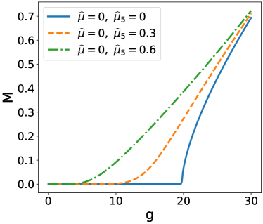
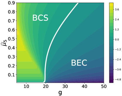
Figure 1: Dynamical mass (left) and the phase diagram (right) for $\mu=0$ at zero temperature. In the right plot, the color scale represents $\log(\widehat{\mu}_{5}/M)$. The white curve indicates $\log(\widehat{\mu}_{5}/M)=0$.

What is the distinction between the BCS regime and the BEC regime? In nonrelativistic systems the unitarity limit marks a crisp boundary, but what about relativistic systems? The locus of a “transition” between the two regimes is not uniquely defined. As suggested in He:2013gga , one popular criterion is to see the dispersion relation $E(\mathbf{p})$ of quasiparticles. If $E(\mathbf{p})$ takes a minimum at $|\mathbf{p}|\approx p_{\text{F}}$, it is in the BCS regime, and if $E(\mathbf{p})$ is a monotonically increasing function of $|\mathbf{p}|$, it is in the BEC regime. This works pretty well in dense QCD where $E(\mathbf{p})=\sqrt{(\sqrt{\mathbf{p}^{2}+M^{2}}-\mu)^{2}+\Delta^{2}}$ (with $\Delta$ the superconducting gap) experiences such a transition when the dynamical mass $M$ is equal to $\mu$. In the current model, however, the dispersion (6) takes a minimum at $|\mathbf{p}|=\mu_{5}$ regardless of the dynamical mass. Yet another criterion is to compare the interparticle distance and the size of Cooper pairs. If the wave function of Cooper pairs extends beyond the average interparticle distance, it is in the BCS regime, otherwise in the BEC regime. In Abuki:2001be ; Itakura:2002vr the size of Cooper pairs in relativistic color superconductors was computed as a function of the quark density and such a BCS-BEC-type crossover was indicated. Unfortunately, a similar analysis is difficult for our model because the interaction is pointlike and the gap has no momentum dependence. As a rule of thumb, let us take the inverse of $M$ as the size of a Cooper pair, and take the inverse of $\mu_{5}$ as the average inter-quark distance. Then the region with $1/M>1/\widehat{\mu}_{5}$ ($1/M<1/\widehat{\mu}_{5}$) corresponds to the BCS (BEC) regime, respectively. According to this crude estimate we labeled each regime in the right plot of Figure 1.

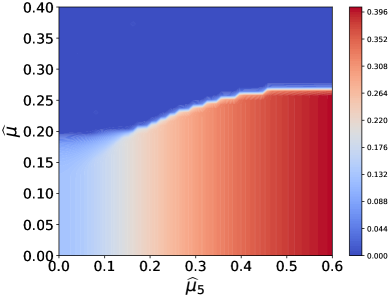
Figure 2: Phase diagrams for $g=17.5$ (left) and $g=20.5$ (right) at zero temperature. The color scale represents $M$.

Next we proceed to the analysis for nonzero $\widehat{\mu}$. The phase diagrams are shown in Figure 2. The main observation here is that for any $\widehat{\mu}_{5}$, there is a critical $\widehat{\mu}$ beyond which the chiral symmetry is restored. This is because $\widehat{\mu}$ induces a mismatch of Fermi surfaces and disrupts Cooper pairing. The critical value of $\widehat{\mu}$ is known as the Chandrasekhar-Clogston limit Chandrasekhar1962 ; Clogston1962 . Analogous situations arise in both condensed matter Radzihovsky_2010 ; Chevy_2010 and high-density QCD Alford:2000ze ; Splittorff:2000mm ; Bedaque:2001je ; Casalbuoni:2003wh ; Nickel:2009wj ; Buballa:2014tba . When the ordinary isotropic Cooper pairing is hampered, a nonstandard pairing that breaks translation symmetry is likely to set in, though it is beyond the scope of this paper.

4 Phase diagram for complex coupling

Finally we complexify the coupling constant. Throughout this section we set $\widehat{\mu}=0$ to simplify the ensuing numerical analysis. Eq. (8) reduces to

$$S =\frac{M^{2}}{2g}-\frac{t}{\pi^{2}}\int_{0}^{1}\mathrm{d}x\;x^{2}\Bigg{[}\log\cosh\left(\frac{\sqrt{(x+\widehat{\mu}_{5})^{2}+M^{2}}}{2t}\right)+\log\cosh\left(\frac{\sqrt{(x-\widehat{\mu}_{5})^{2}+M^{2}}}{2t}\right)\Bigg{]}$$ (10)

where $g\in\mathbb{C}$ and $M\in\mathbb{C}$. When $M$ is purely imaginary, $\sqrt{(x\pm\widehat{\mu}_{5})^{2}+M^{2}}$ may be exactly on the branch cut of the complex square root, which makes the zero-temperature limit $t\to+0$ ill-defined. When $M$ is not purely imaginary, we have for $t\to+0$

$$S =\frac{M^{2}}{2g}-\frac{1}{2\pi^{2}}\int_{0}^{1}\mathrm{d}x\;x^{2}\big{[}\sqrt{(x+\widehat{\mu}_{5})^{2}+M^{2}}+\sqrt{(x-\widehat{\mu}_{5})^{2}+M^{2}}\big{]}\,.$$ (11)

This integral can be performed with the formula

$$\int\mathrm{d}x\;x^{2}\sqrt{(x+\mu)^{2}+M^{2}} =-\frac{M^{2}(M^{2}-4\mu^{2})}{8}\tanh^{-1}\left(\frac{x+\mu}{\sqrt{(x+\mu)^{2}+M^{2}}}\right)$$

$$\quad+\frac{\sqrt{(x+\mu)^{2}+M^{2}}}{24}\left[6x^{3}+2\mu x^{2}+(3M^{2}-2\mu^{2})x+2\mu^{3}-13M^{2}\mu\right]$$

$$=:F(x,\mu,M)\,,$$ (12)

where $\tanh^{-1}(z)=\frac{1}{2}\log\left(\frac{1+z}{1-z}\right)$ is the inverse function of $\tanh(z)$. This way we obtain

$$S =\frac{M^{2}}{2g}-\frac{1}{2\pi^{2}}\left[F(1,\widehat{\mu}_{5},M)-F(0,\widehat{\mu}_{5},M)+F(1,-\widehat{\mu}_{5},M)-F(0,-\widehat{\mu}_{5},M)\right]$$ (13)

$$=\frac{M^{2}}{2g}-\frac{1}{2\pi^{2}}\Bigg{[}-\frac{M^{2}(M^{2}-4\widehat{\mu}_{5}^{2})}{8}\Bigg{\{}\tanh^{-1}\left(\frac{1+\widehat{\mu}_{5}}{\sqrt{(1+\widehat{\mu}_{5})^{2}+M^{2}}}\right)$$

$$\quad+\tanh^{-1}\left(\frac{1-\widehat{\mu}_{5}}{\sqrt{(1-\widehat{\mu}_{5})^{2}+M^{2}}}\right)\Bigg{\}}$$

$$\quad+\frac{\sqrt{(1+\widehat{\mu}_{5})^{2}+M^{2}}}{24}(6+2\widehat{\mu}_{5}+3M^{2}-2\widehat{\mu}_{5}^{2}+2\widehat{\mu}_{5}^{3}-13M^{2}\widehat{\mu}_{5})$$

$$\quad+\frac{\sqrt{(1-\widehat{\mu}_{5})^{2}+M^{2}}}{24}(6-2\widehat{\mu}_{5}+3M^{2}-2\widehat{\mu}_{5}^{2}-2\widehat{\mu}_{5}^{3}+13M^{2}\widehat{\mu}_{5})\Bigg{]}\,.$$ (14)

Since $S$ is a function of $M^{2}$, the trivial vacuum $M=0$ is always a solution to $\partial S/\partial M=0$. We are interested in the gap equation for $M\neq 0$, which reads

$$0 \overset{!}{=}\frac{1}{2M}\frac{\partial S}{\partial M}$$

$$=\frac{1}{2g}+\frac{1}{8\pi^{2}}\Bigg{[}(3\widehat{\mu}_{5}-1)\sqrt{(1+\widehat{\mu}_{5})^{2}+M^{2}}-(3\widehat{\mu}_{5}+1)\sqrt{(1-\widehat{\mu}_{5})^{2}+M^{2}}$$

$$\quad+(M^{2}-2\widehat{\mu}_{5}^{2})\left\{\tanh^{-1}\left(\frac{1+\widehat{\mu}_{5}}{\sqrt{(1+\widehat{\mu}_{5})^{2}+M^{2}}}\right)+\tanh^{-1}\left(\frac{1-\widehat{\mu}_{5}}{\sqrt{(1-\widehat{\mu}_{5})^{2}+M^{2}}}\right)\right\}\Bigg{]}\,.$$ (15)

We have varied $g$ on the complex plane and numerically searched for a solution to (15) for each $g$. It turned out that there was no solution for $\mathrm{Re}\;g<0$, indicating that chiral symmetry is unbroken for $\mathrm{Re}\;g<0$. This is natural because $\mathrm{Re}\;g<0$ is a repulsive interaction. Furthermore, the phase structures for $\mathrm{Im}\;g>0$ and $\mathrm{Im}\;g<0$ are symmetric about the real axis of $g$. Hence we will assume $\mathrm{Re}\;g>0$ and $\mathrm{Im}\;g>0$ in the following.

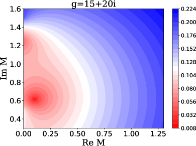
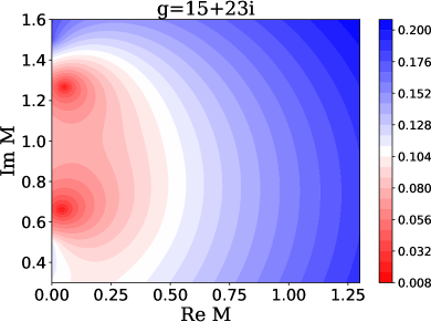
Figure 3: $\sqrt{|\partial S/\partial M|}$ on the complex $M$ plane at $\widehat{\mu}_{5}=0.5$ for three values of complex $g$.

By monitoring the magnitude of the gradient $\partial S/\partial M$ we found an interesting mechanism that changes the number of saddle points of $S$. In Figure 3(a), (b) and (c) we display $\sqrt{|\partial S/\partial M|}$ as a function of $M$ for three values of $g$. (The square root of the gradient was taken for better visibility of the figures.) In Figure 3(a) there is only one saddle point. (Of course there is another saddle for $M\to-M$.) When we increase the imaginary part of $g$, as shown in Figure 3(b), a new saddle point is suddenly born out of the imaginary axis of $M$. So there are now two saddle points. When the imaginary part of $g$ is further increased, as shown in Figure 3(c), the old saddle is absorbed into the imaginary axis and we are left with a single saddle. In this fashion the number of saddles (i.e., the solutions to (15)) can jump abruptly.

When there are multiple saddles, the dominant one is definitely the one that has the lowest value of $\mathrm{Re}\,S$, since it has the largest magnitude of $\operatorname{\mathrm{e}}^{-S}$ and dominates the partition function as a sum over saddles $Z\approx\sum_{n}c_{n}\operatorname{\mathrm{e}}^{-S_{n}}$ provided that all $c_{n}$’s are of the same order. Following UedaPRL2019 ; Iskin2020 , we define three phases as below.

• Normal phase: (15) has no solution, i.e., $M=0$ is the only saddle of $S$.

• Metastable $\chi$SB phase: there are solutions to (15), but their $\mathrm{Re}\;S$ are higher than that for $M=0$.

• Stable $\chi$SB phase: there are solutions to (15) whose $\mathrm{Re}\;S$ are lower than that for $M=0$.

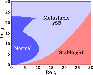
Figure 4: The phase diagram for $\widehat{\mu}_{5}=0.5$ (left) and the magnitude of the complex dynamical mass $|M|$ (right). The dashed black line represents $|M|=\widehat{\mu}_{5}$.

In Figure 4 (left) we display the phase diagram for $\widehat{\mu}_{5}=0.5$ on the complex $g$ plane. In the vicinity of the real axis we have a stable $\chi$SB phase. As $\mathrm{Im}\;g$ increases, we are driven into a metastable $\chi$SB phase via a quantum phase transition. At small $\mathrm{Re}\;g$ the metastable saddle goes away and the chiral symmetry is completely restored. Interestingly, as one goes up along the imaginary axis, a metastable $\chi$SB state emerges suddenly at $\mathrm{Im}\;g\simeq 22.5$; this means that a very strong dissipation can trigger $\chi$SB (albeit a metastable one). The global phase structure we found here is quite similar to the one for nonrelativistic fermions on a lattice UedaPRL2019 , though we note that the phase diagram at small $\mathrm{Re}\;g$ was not presented in UedaPRL2019 because of the limitation of numerical calculations. (See section 5 where we argue that part of the features of this phase diagram can be attributed to the usage of a sharp momentum cutoff.)

To gain more insights, in Figure 4 (right) we plot the magnitude of the gap $|M|$. When there are multiple saddles, we took the one that has the lowest $\mathrm{Re}\;S$. Notice that nothing dramatic happens at the boundary between the metastable $\chi$SB phase and the stable $\chi$SB phase. It is worth noting that the gap magnitude tends to be enhanced by dissipation. As a crude guide we drew the boundary $|M|\sim\widehat{\mu}_{5}$ between the BCS regime and the BEC regime. We emphasize that this is a rule of thumb and a more rigorous characterization of the crossover region in non-Hermitian superfluids is left as an open problem. We point out that for $\mathrm{Im}\;g\gtrsim 20$ the gap reaches the UV cutoff scale ($|M|\sim 1$); this implies that all the calculations for $\mathrm{Im}\;g\gtrsim 20$ are extremely sensitive to the regularization scheme used, and hence one has to be careful about physical interpretations.

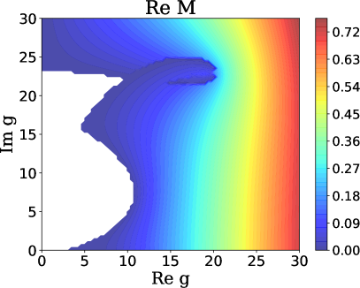
Figure 5: The real and imaginary parts of the complex dynamical mass $M$ for $\widehat{\mu}_{5}=0.5$.

Figure 5 shows the real and imaginary parts of $M$. The left panel shows that $\mathrm{Re}\;M$ grows monotonically with $\mathrm{Re}\;g$ and is largely independent of $\mathrm{Im}\;g$. Note that $\mathrm{Re}\;M$ approaches zero along the boundary with the normal phase. This means that, when one moves out of the normal phase, a nontrivial solution to the gap equation emerges out of the imaginary axis of $M$. The right panel shows that $\mathrm{Im}\;M$ grows monotonically with $\mathrm{Im}\;g$.

It is instructive to compare our findings with preceding works.

• Ref. UedaPRL2019 found an enhancement of superfluidity by dissipation, and attributed it to the continuous quantum Zeno effect which suppresses tunneling and reinforces on-site molecule formation. This effect is unique to a lattice system. Nevertheless we observed a similar enhancement in a continuum model; we speculate that the presence of a sharp momentum cutoff plays a role similar to that of a lattice. See section 5 for a discussion on an alternative UV regularization.

• Ref. Iskin2020 solved the BCS-BEC crossover for a complex scattering length and found that the superfluid phase is stable even in the limit of strong dissipation, which is surprising. The difference of Iskin2020 from UedaPRL2019 and this paper may be due to the fact that Iskin2020 considered a complex-valued chemical potential.

• Ref. Zhou2018 reports that a non-Hermitian perturbation (an imaginary magnetic field) enhances superfluidity.

• Ref. Felski:2020vrm solved the NJL model supplemented with a non-Hermitian bilinear term that preserves chiral symmetry. It was found that, as the non-Hermitian coupling grows, the dynamical mass first rises and then drops to zero.

Finally we turn to the quasiparticle excitation spectra $E(\mathbf{p})=\sqrt{(|\mathbf{p}|/\Lambda-\widehat{\mu}_{5})^{2}+M^{2}}$ which is generally complex for complex $g$. The real and (scaled) imaginary parts of $E(\mathbf{p})$ are displayed in Figure 6. At weak coupling, the imaginary part of $E(\mathbf{p})$ is sharply concentrated around the Fermi level (left panel). By contrast, at stronger coupling, the imaginary part has a much broader support (right panel). These are results for weak dissipation ($\mathrm{Im}\;g=0.5$). If dissipation is stronger, a more peculiar thing can occur: at the boundary between the normal phase and the metastable $\chi$SB phase, $M$ is purely imaginary (cf. Figure 5), hence $E(\mathbf{p})$ is purely imaginary for $\widehat{\mu}_{5}-|M|\leq|\mathbf{p}|/\Lambda\leq\widehat{\mu}_{5}+|M|$ and is real otherwise. The bounds $|\mathbf{p}|/\Lambda=\widehat{\mu}_{5}\pm|M|$ are an example of the so-called exceptional points Heiss_2012 where the dimensionality of the eigenspace of the Hamiltonian decreases.

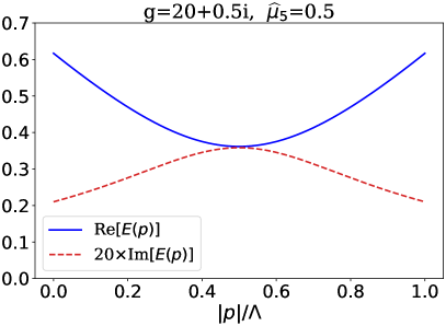
Figure 6: The complex energy spectra of quasiparticles for weak (left) and strong (right) coupling.

5 Dependence on the UV regularization scheme

In this section, we investigate what happens to the phase diagram when the sharp momentum cutoff used in section 4 is replaced with a more smooth UV regulator. Since the numerical search of a solution to the gap equation requires high numerical precision, it is mandatory to choose a regulator such that the momentum integral for the action $S$ can be evaluated analytically. For this reason, we choose smooth form factors

$$\frac{1}{\left[\displaystyle 1+\left(\frac{|\mathbf{p}|+\mu_{5}}{\Lambda}\right)^{2}\right]^{3}}\qquad\text{and}\qquad\frac{1}{\left[\displaystyle 1+\left(\frac{|\mathbf{p}|-\mu_{5}}{\Lambda}\right)^{2}\right]^{3}}\,.$$ (16)

Then the action, in dimensionless form, reads as

$$S =\frac{M^{2}}{2g}-\frac{1}{2\pi^{2}}\int_{0}^{\infty}\mathrm{d}x\;x^{2}\left\{\frac{\sqrt{(x+\widehat{\mu}_{5})^{2}+M^{2}}}{[1+\left(x+\widehat{\mu}_{5}\right)^{2}]^{3}}+\frac{\sqrt{(x-\widehat{\mu}_{5})^{2}+M^{2}}}{[1+\left(x-\widehat{\mu}_{5}\right)^{2}]^{3}}\right\}$$ (17)

$$=\frac{M^{2}}{2g}-\frac{1}{4\pi^{2}}\int_{-\infty}^{\infty}\mathrm{d}x\;x^{2}\left\{\frac{\sqrt{(x+\widehat{\mu}_{5})^{2}+M^{2}}}{[1+\left(x+\widehat{\mu}_{5}\right)^{2}]^{3}}+\frac{\sqrt{(x-\widehat{\mu}_{5})^{2}+M^{2}}}{[1+\left(x-\widehat{\mu}_{5}\right)^{2}]^{3}}\right\}$$ (18)

$$=\frac{M^{2}}{2g}-\frac{1}{4\pi^{2}}\int_{-\infty}^{\infty}\mathrm{d}x\;[(x-\widehat{\mu}_{5})^{2}+(x+\widehat{\mu}_{5})^{2}]\frac{\sqrt{x^{2}+M^{2}}}{(1+x^{2})^{3}}$$ (19)

$$=\frac{M^{2}}{2g}-\frac{1}{2\pi^{2}}\int_{-\infty}^{\infty}\mathrm{d}x\;(x^{2}+\widehat{\mu}_{5}^{2})\frac{\sqrt{x^{2}+M^{2}}}{(1+x^{2})^{3}}$$ (20)

$$=\frac{M^{2}}{2g}-\frac{1}{2\pi^{2}}\frac{\sqrt{M^{2}-1}\left[M^{2}-2+(3M^{2}-2)\widehat{\mu}_{5}^{2}\right]+M^{2}\left[M^{2}+(3M^{2}-4)\widehat{\mu}_{5}^{2}\right]\mathrm{ArcSec}\sqrt{M^{2}}}{4(M^{2}-1)^{3/2}}.$$ (21)

Then we have for the gradient

$$\scalebox{0.85}{$\displaystyle\frac{1}{2M}\frac{\partial S}{\partial M}=\frac{1}{2g}-\frac{\sqrt{M^{2}-1}\left[M^{2}+2+3(M^{2}-2)\widehat{\mu}_{5}^{2}\right]+\left\{M^{2}(M^{2}-4)+\left[M^{2}(3M^{2}-8)+8\right]\widehat{\mu}_{5}^{2}\right\}\mathrm{ArcSec}\sqrt{M^{2}}}{16\pi^{2}(M^{2}-1)^{5/2}}$}.$$ (22)

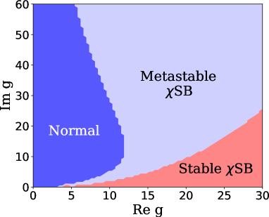
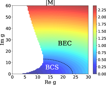
Figure 7: Same as Figure 4 but with a smooth UV regularization using the form factor (16). Note that the vertical scale is twice larger than Figure 4.

We numerically searched for a solution to (22) with varying $g\in\mathbb{C}$ and, if there was any solution, investigated its stability as compared to the trivial vacuum $M=0$. The result is shown in Figure 7. It is clear that the normal phase without a metastable vacuum has expanded substantially in comparison to Figure 4. It is thus concluded that the emergence of a metastable $\chi$SB phase in the region $\text{Re}\;g\ll\text{Im}\;g$ in Figure 4 is largely an artifact due to the sharp momentum cutoff.

6 Conclusions and outlook

In summary, we have investigated $\chi$SB of Dirac fermions in four dimensions at finite chiral chemical potential for a complex-valued four-fermion coupling. We varied the coupling over the entire range from the weakly bound BCS regime to the tightly bound BEC regime, and numerically constructed the phase diagram. Our primary result is that the imaginary coupling tends to enhance $\chi$SB up to a certain threshold; when the imaginary coupling exceeds the threshold, the chiral symmetry is restored, although a nontrivial solution to the gap equation continues to exist. We illustrated how complex saddles of the action come into existence and go away through the imaginary axis of the complex gap plane along which the action has a branch cut. We also worked out the complex energy spectra of quasiparticles. Our results can in principle be tested in experiments using ultracold atomic gases and other materials that host Dirac fermions Vafek:2013mpa ; Wehling_2014 ; Armitage:2017cjs . However, it may be difficult to draw implications for quark matter in compact stars from this work, because the pointlike four-fermion interaction is a very crude approximation to the non-Abelian gauge interaction between quarks.

There are miscellaneous future directions in which this work can be extended. A partial list is given below.

• To incorporate the competition between the chiral condensate and the diquark condensate (i.e., a competition between a Dirac mass and a Majorana mass) along the lines of Berges:1998rc ; Ratti:2004ra

• To investigate collective fluctuations around the saddle points and test the validity of the mean-field approximation for non-Hermitian $\chi$SB

• To analytically prove numerical findings in this work, e.g., the existence of a nontrivial solution to the gap equation for large $\mathrm{Im}\;g$

• To examine dissipative $\chi$SB under an external magnetic field that catalyzes $\chi$SB Andersen:2014xxa ; Miransky:2015ava

• To study $\text{U}(1)_{A}$ vortices

• To study the effect of nonzero $\mu$ on non-Hermitian $\chi$SB

• To analyze the structure of Cooper pairs as a function of the complex coupling, and provide a more precise description of the non-Hermitian BCS-BEC crossover

• To use the renormalization group to improve the mean-field analysis

• To clarify how to apply the Lefschetz thimble approach Alexandru:2020wrj to non-Hermitian $\chi$SB where the complex action and its gradient have branch cuts

• To use the results of this paper to benchmark algorithms (such as the complex Langevin method Aarts:2009uq ) for simulating complex-action theories

• To extend this work to lower spatial dimensions

• To test the conclusions of this paper with other low-energy effective models such as holography Herzog:2009xv (see Arean:2019pom for a non-Hermitian extension)

References

- (1) N. Moiseyev, Non-Hermitian Quantum Mechanics, Cambridge University Press (2011), 10.1017/CBO9780511976186.
- (2) Y. Ashida, Z. Gong and M. Ueda, Non-Hermitian Physics, 2006.01837.
- (3) J. Dalibard, Y. Castin and K. Molmer, Wave-function approach to dissipative processes in quantum optics, Phys. Rev. Lett. 68 (1992) 580.
- (4) H.J. Carmichael, Quantum trajectory theory for cascaded open systems, Phys. Rev. Lett. 70 (1993) 2273.
- (5) A.J. Daley, Quantum trajectories and open many-body quantum systems, Adv. Phys. 63 (2014) 77 [1405.6694].
- (6) C.M. Bender and S. Boettcher, Real Spectra in Non-Hermitian Hamiltonians Having PT Symmetry, Phys. Rev. Lett. 80 (1998) 5243 [physics/9712001].
- (7) C.M. Bender, D.C. Brody and H.F. Jones, Complex extension of quantum mechanics, Phys. Rev. Lett. 89 (2002) 270401 [quant-ph/0208076].
- (8) C.M. Bender, Making sense of non-Hermitian Hamiltonians, Rept. Prog. Phys. 70 (2007) 947 [hep-th/0703096].
- (9) Y. Takasu, T. Yagami, Y. Ashida, R. Hamazaki, Y. Kuno and Y. Takahashi, PT-symmetric non-Hermitian quantum many-body system using ultracold atoms in an optical lattice with controlled dissipation, Prog. Theor. Exp. Phys. 2020 (2020) 12A110 [2004.05734].
- (10) D. Bernard and A. LeClair, A Classification of Non-Hermitian Random Matrices, in Statistical Field Theories. NATO Science Series (Series II: Mathematics, Physics and Chemistry), A. Cappelli and G. Mussardo, eds., vol. 73, pp. 207–214, Springer, Dordrecht, 2002, DOI [cond-mat/0110649].
- (11) K. Kawabata, K. Shiozaki, M. Ueda and M. Sato, Symmetry and Topology in Non-Hermitian Physics, Phys. Rev. X 9 (2019) 041015 [1812.09133].
- (12) V.M. Martinez Alvarez, J.E. Barrios Vargas and L.E.F. Foa Torres, Non-Hermitian robust edge states in one dimension: Anomalous localization and eigenspace condensation at exceptional points, Phys. Rev. B 97 (2018) 121401 [1711.05235].
- (13) S. Yao and Z. Wang, Edge States and Topological Invariants of Non-Hermitian Systems, Phys. Rev. Lett. 121 (2018) 086803 [1803.01876].
- (14) V.M. Martinez Alvarez, J.E. Barrios Vargas, M. Berdakin and L.E.F. Foa Torres, Topological states of non-Hermitian systems, Eur. Phys. J. Special Topics 227 (2018) 1295 [1805.08200].
- (15) D.S. Borgnia, A.J. Kruchkov and R.-J. Slager, Non-Hermitian Boundary Modes and Topology, Phys. Rev. Lett. 124 (2020) 056802 [1902.07217].
- (16) N. Okuma, K. Kawabata, K. Shiozaki and M. Sato, Topological Origin of Non-Hermitian Skin Effects, Phys. Rev. Lett. 124 (2020) 086801 [1910.02878].
- (17) N. Hatano and D.R. Nelson, Localization Transitions in Non-Hermitian Quantum Mechanics, Phys. Rev. Lett. 77 (1996) 570 [cond-mat/9603165].
- (18) A. Rothkopf, T. Hatsuda and S. Sasaki, Complex Heavy-Quark Potential at Finite Temperature from Lattice QCD, Phys. Rev. Lett. 108 (2012) 162001 [1108.1579].
- (19) A. Rothkopf, Heavy Quarkonium in Extreme Conditions, Phys. Rept. 858 (2020) 1 [1912.02253].
- (20) Y. Akamatsu, Quarkonium in Quark-Gluon Plasma: Open Quantum System Approaches Re-examined, 2009.10559.
- (21) M.N. Chernodub and A. Cortijo, Non-Hermitian Chiral Magnetic Effect in Equilibrium, Symmetry 12 (2020) 761 [1901.06167].
- (22) A. Denbleyker, D. Du, Y. Meurice and A. Velytsky, Fisher’s Zeros and Perturbative Series in Gluodynamics, PoS LATTICE2007 (2007) 269 [0710.5771].
- (23) A. Denbleyker, D. Du, Y. Liu, Y. Meurice and H. Zou, Fisher’s zeros as boundary of renormalization group flows in complex coupling spaces, Phys. Rev. Lett. 104 (2010) 251601 [1005.1993].
- (24) Y. Meurice and H. Zou, Complex RG flows for 2D nonlinear O(N) sigma models, Phys. Rev. D 83 (2011) 056009 [1101.1319].
- (25) Y. Liu and Y. Meurice, Lines of Fisher’s zeros as separatrices for complex renormalization group flows, Phys. Rev. D 83 (2011) 096008 [1103.4846].
- (26) A. Denbleyker, A. Bazavov, D. Du, Y. Liu, Y. Meurice and H. Zou, Fisher’s zeros, complex RG flows and confinement in LGT models, PoS LATTICE2011 (2011) 299 [1112.2734].
- (27) A. Bazavov, B. Berg, D. Du and Y. Meurice, Density of states and Fisher’s zeros in compact U(1) pure gauge theory, Phys. Rev. D 85 (2012) 056010 [1202.2109].
- (28) C.M. Bender, H. Jones and R. Rivers, Dual PT-symmetric quantum field theories, Phys. Lett. B 625 (2005) 333 [hep-th/0508105].
- (29) J. Alexandre, C.M. Bender and P. Millington, Non-Hermitian extension of gauge theories and implications for neutrino physics, JHEP 11 (2015) 111 [1509.01203].
- (30) J. Alexandre, P. Millington and D. Seynaeve, Symmetries and conservation laws in non-Hermitian field theories, Phys. Rev. D 96 (2017) 065027 [1707.01057].
- (31) A. Beygi, S. Klevansky and C.M. Bender, Relativistic -symmetric fermionic theories in 1+1 and 3+1 dimensions, Phys. Rev. A 99 (2019) 062117 [1904.00878].
- (32) J. Alexandre, J. Ellis and P. Millington, -symmetric non-Hermitian quantum field theories with supersymmetry, Phys. Rev. D 101 (2020) 085015 [2001.11996].
- (33) J. Alexandre and N.E. Mavromatos, On the consistency of a non-Hermitian Yukawa interaction, Phys. Lett. B 807 (2020) 135562 [2004.03699].
- (34) A. Felski, A. Beygi and S. Klevansky, Non-Hermitian extension of the Nambu–Jona-Lasinio model in 3+1 and 1+1 dimensions, Phys. Rev. D 101 (2020) 116001 [2004.04011].
- (35) J. Alexandre, N.E. Mavromatos and A. Soto, Dynamical Majorana Neutrino Masses and Axions, Nucl. Phys. B 961 (2020) 115212 [2004.04611].
- (36) N.E. Mavromatos and A. Soto, Dynamical Majorana Neutrino Masses and Axions II: Inclusion of Axial Background and Anomaly Terms, Nucl. Phys. B 962 (2021) 115275 [2006.13616].
- (37) M. Chernodub, A. Cortijo and M. Ruggieri, Spontaneous Non-Hermiticity in Nambu-Jona-Lasinio model, 2008.11629.
- (38) Y. Nambu and G. Jona-Lasinio, Dynamical Model of Elementary Particles Based on an Analogy with Superconductivity. I, Phys. Rev. 122 (1961) 345.
- (39) Y. Nambu and G. Jona-Lasinio, Dynamical Model of Elementary Particles Based on an Analogy with Superconductivity. II, Phys. Rev. 124 (1961) 246.
- (40) S. Klevansky, The Nambu-Jona-Lasinio model of quantum chromodynamics, Rev. Mod. Phys. 64 (1992) 649.
- (41) T. Hatsuda and T. Kunihiro, QCD phenomenology based on a chiral effective Lagrangian, Phys. Rept. 247 (1994) 221 [hep-ph/9401310].
- (42) M. Buballa, NJL model analysis of quark matter at large density, Phys. Rept. 407 (2005) 205 [hep-ph/0402234].
- (43) G. Guralnik and Z. Guralnik, Complexified path integrals and the phases of quantum field theory, Annals Phys. 325 (2010) 2486 [0710.1256].
- (44) G. Alexanian, R. MacKenzie, M. Paranjape and J. Ruel, Path integration and perturbation theory with complex Euclidean actions, Phys. Rev. D 77 (2008) 105014 [0802.0354].
- (45) E. Witten, Analytic Continuation Of Chern-Simons Theory, AMS/IP Stud. Adv. Math. 50 (2011) 347 [1001.2933].
- (46) AuroraScience collaboration, New approach to the sign problem in quantum field theories: High density QCD on a Lefschetz thimble, Phys. Rev. D 86 (2012) 074506 [1205.3996].
- (47) H. Fujii, D. Honda, M. Kato, Y. Kikukawa, S. Komatsu and T. Sano, Hybrid Monte Carlo on Lefschetz thimbles - A study of the residual sign problem, JHEP 10 (2013) 147 [1309.4371].
- (48) Y. Tanizaki and T. Koike, Real-time Feynman path integral with Picard–Lefschetz theory and its applications to quantum tunneling, Annals Phys. 351 (2014) 250 [1406.2386].
- (49) T. Kanazawa and Y. Tanizaki, Structure of Lefschetz thimbles in simple fermionic systems, JHEP 03 (2015) 044 [1412.2802].
- (50) Y. Tanizaki, Y. Hidaka and T. Hayata, Lefschetz-thimble analysis of the sign problem in one-site fermion model, New J. Phys. 18 (2016) 033002 [1509.07146].
- (51) H. Fujii, S. Kamata and Y. Kikukawa, Monte Carlo study of Lefschetz thimble structure in one-dimensional Thirring model at finite density, JHEP 12 (2015) 125 [1509.09141].
- (52) A. Alexandru, G. Basar, P.F. Bedaque, G.W. Ridgway and N.C. Warrington, Sign problem and Monte Carlo calculations beyond Lefschetz thimbles, JHEP 05 (2016) 053 [1512.08764].
- (53) A. Alexandru, G. Basar and P. Bedaque, Monte Carlo algorithm for simulating fermions on Lefschetz thimbles, Phys. Rev. D 93 (2016) 014504 [1510.03258].
- (54) Y. Mori, K. Kashiwa and A. Ohnishi, Toward solving the sign problem with path optimization method, Phys. Rev. D 96 (2017) 111501 [1705.05605].
- (55) A. Alexandru, P.F. Bedaque, H. Lamm and S. Lawrence, Deep Learning Beyond Lefschetz Thimbles, Phys. Rev. D 96 (2017) 094505 [1709.01971].
- (56) M. Fukuma, N. Matsumoto and N. Umeda, Applying the tempered Lefschetz thimble method to the Hubbard model away from half-filling, Phys. Rev. D 100 (2019) 114510 [1906.04243].
- (57) Z.-G. Mou, P.M. Saffin and A. Tranberg, Quantum tunnelling, real-time dynamics and Picard-Lefschetz thimbles, JHEP 11 (2019) 135 [1909.02488].
- (58) A. Alexandru, G. Basar, P.F. Bedaque and N.C. Warrington, Complex Paths Around The Sign Problem, 2007.05436.
- (59) H. Markum, R. Pullirsch and T. Wettig, NonHermitian random matrix theory and lattice QCD with chemical potential, Phys. Rev. Lett. 83 (1999) 484 [hep-lat/9906020].
- (60) B.A. Khoruzhenko and H.J. Sommers, Non-Hermitian Random Matrix Ensembles, 0911.5645.
- (61) T. Kanazawa, Dirac Spectra in Dense QCD, Springer Japan (2013).
- (62) A.J. Leggett, Quantum Liquids: Bose condensation and Cooper pairing in condensed-matter systems, Oxford University Press (2006).
- (63) R. Casalbuoni, Lecture Notes on Superconductivity: Condensed Matter and QCD, 1810.11125.
- (64) N.M. Chtchelkatchev, A.A. Golubov, T.I. Baturina and V.M. Vinokur, Stimulation of the Fluctuation Superconductivity by PT Symmetry, Phys. Rev. Lett. 109 (2012) 150405 [arXiv:1008.3590].
- (65) A. Ghatak and T. Das, Theory of superconductivity with non-Hermitian and parity-time reversal symmetric Cooper pairing symmetry, Phys. Rev. B 97 (2018) 014512 [arXiv:1708.09108].
- (66) L. Zhou and X. Cui, Enhanced fermion pairing and superfluidity by an imaginary magnetic field, iScience 14 (2019) 257 [1812.11008].
- (67) K. Yamamoto, M. Nakagawa, K. Adachi, K. Takasan, M. Ueda and N. Kawakami, Theory of Non-Hermitian Fermionic Superfluidity with a Complex-Valued Interaction, Phys. Rev. Lett. 123 (2019) 123601 [arXiv:1903.04720].
- (68) M. Iskin, Non-Hermitian BCS-BEC evolution with a complex scattering length, Phys. Rev. A 103 (2020) 013724 [2002.00653].
- (69) J.M. Blatt, K.W. Böer and W. Brandt, Bose-Einstein Condensation of Excitons, Phys. Rev. 126 (1962) 1691.
- (70) K. Yoshioka, E. Chae and M. Kuwata-Gonokami, Transition to a Bose-Einstein condensate and relaxation explosion of excitons at sub-Kelvin temperatures, Nature Communications 2 (2011) 328 [1008.2431].
- (71) T. Ogawa, Y. Tomio and K. Asano, Quantum condensation in electron-hole systems: excitonic BEC-BCS crossover and biexciton crystallization, J. Phys.: Condens. Matter 19 (2007) 295205.
- (72) M. Yamaguchi, K. Kamide, T. Ogawa and Y. Yamamoto, BEC-BCS-laser crossover in Coulomb-correlated electron-hole-photon systems, New J. Phys. 14 (2012) 065001.
- (73) R. Hanai, P.B. Littlewood and Y. Ohashi, Non-equilibrium Properties of a Pumped-Decaying Bose-Condensed Electron-Hole Gas in the BCS-BEC Crossover Region, J. Low Temp. Phys. 183 (2016) 127 [1506.08983].
- (74) R. Hanai, P.B. Littlewood and Y. Ohashi, Dynamical instability of a driven-dissipative electron-hole condensate in the BCS-BEC crossover region, Phys. Rev. B 96 (2017) 125206 [1610.08622].
- (75) T. Kawamura, D. Kagamihara, R. Hanai and Y. Ohashi, Strong-Coupling Theory for a Non-equilibrium Unitary Fermi Gas, J. Low Temp. Phys. (2019) .
- (76) T. Kawamura, R. Hanai, D. Kagamihara, D. Inotani and Y. Ohashi, Nonequilibrium strong-coupling theory for a driven-dissipative ultracold Fermi gas in the BCS-BEC crossover region, Phys. Rev. A 101 (2020) 013602 [1910.12476].
- (77) C. Triola, A. Pertsova, R.S. Markiewicz and A.V. Balatsky, Excitonic gap formation in pumped Dirac materials, Phys. Rev. B 95 (2017) 205410 [1701.04206].
- (78) A. Pertsova and A.V. Balatsky, Excitonic instability in optically pumped three-dimensional Dirac materials, Phys. Rev. B 97 (2018) 075109 [1710.09132].
- (79) A. Pertsova and A.V. Balatsky, Dynamically Induced Excitonic Instability in Pumped Dirac Materials, Annalen der Physik 532 (2020) 1900549 [1912.09400].
- (80) P. Nozières and S. Schmitt-Rink, Bose condensation in an attractive fermion gas: From weak to strong coupling superconductivity, Journal of Low Temperature Physics 59 (1985) 195.
- (81) Q. Chen, J. Stajic, S. Tan and K. Levin, BCS-BEC crossover: From high temperature superconductors to ultracold superfluids, Physics Reports 412 (2005) 1 [arXiv:cond-mat/0404274].
- (82) S. Giorgini, L.P. Pitaevskii and S. Stringari, Theory of ultracold atomic Fermi gases, Rev. Mod. Phys. 80 (2008) 1215 [arXiv:0706.3360].
- (83) W. Zwerger, ed., The BCS-BEC Crossover and the Unitary Fermi Gas, Springer (2012), 10.1007/978-3-642-21978-8.
- (84) M. Randeria and E. Taylor, Crossover from Bardeen-Cooper-Schrieffer to Bose-Einstein Condensation and the Unitary Fermi Gas, Annual Review of Condensed Matter Physics 5 (2014) 209 [arXiv:1306.5785].
- (85) G.C. Strinati, P. Pieri, G. Röpke, P. Schuck and M. Urban, The BCS-BEC crossover: From ultra-cold Fermi gases to nuclear systems, Physics Reports 738 (2018) 1 [arXiv:1802.05997].
- (86) S.-L. Zhu, B. Wang and L.-M. Duan, Simulation and Detection of Dirac Fermions with Cold Atoms in an Optical Lattice, Phys. Rev. Lett. 98 (2007) 260402 [cond-mat/0703454].
- (87) L.-K. Lim, A. Lazarides, A. Hemmerich and C. Morais Smith, Strongly interacting two-dimensional Dirac fermions, Europhys. Lett. 88 (2009) 36001 [0905.1281].
- (88) J. Ignacio Cirac, P. Maraner and J.K. Pachos, Cold atom simulation of interacting relativistic quantum field theories, Phys. Rev. Lett. 105 (2010) 190403 [1006.2975].
- (89) Y. Nishida and H. Abuki, BCS-BEC crossover in a relativistic superfluid and its significance to quark matter, Phys. Rev. D 72 (2005) 096004 [hep-ph/0504083].
- (90) H. Abuki, BCS/BEC crossover in Quark Matter and Evolution of its Static and Dynamic properties: From the atomic unitary gas to color superconductivity, Nucl. Phys. A 791 (2007) 117 [hep-ph/0605081].
- (91) J. Deng, A. Schmitt and Q. Wang, Relativistic BCS-BEC crossover in a boson-fermion model, Phys. Rev. D 76 (2007) 034013 [nucl-th/0611097].
- (92) L. He and P. Zhuang, Relativistic BCS-BEC crossover at zero temperature, Phys. Rev. D 75 (2007) 096003 [hep-ph/0703042].
- (93) L. He and P. Zhuang, Relativistic BCS-BEC crossover at finite temperature and Its application to color superconductivity, Phys. Rev. D 76 (2007) 056003 [0705.1634].
- (94) G.-f. Sun, L. He and P. Zhuang, BEC-BCS crossover in the Nambu-Jona-Lasinio model of QCD, Phys. Rev. D 75 (2007) 096004 [hep-ph/0703159].
- (95) T. Brauner, BCS-BEC crossover in dense relativistic matter: Collective excitations, Phys. Rev. D 77 (2008) 096006 [0803.2422].
- (96) B. Chatterjee, H. Mishra and A. Mishra, BCS-BEC crossover and phase structure of relativistic systems: A variational approach, Phys. Rev. D 79 (2009) 014003 [0804.1051].
- (97) L. He, Nambu-Jona-Lasinio model description of weakly interacting Bose condensate and BEC-BCS crossover in dense QCD-like theories, Phys. Rev. D 82 (2010) 096003 [1007.1920].
- (98) T. Kanazawa, T. Wettig and N. Yamamoto, Singular values of the Dirac operator in dense QCD-like theories, JHEP 12 (2011) 007 [1110.5858].
- (99) L. He, S. Mao and P. Zhuang, BCS-BEC crossover in relativistic Fermi systems, Int. J. Mod. Phys. A 28 (2013) 1330054 [1311.6704].
- (100) M.G. Alford, A. Schmitt, K. Rajagopal and T. Schäfer, Color superconductivity in dense quark matter, Rev. Mod. Phys. 80 (2008) 1455 [0709.4635].
- (101) K. Fukushima, D.E. Kharzeev and H.J. Warringa, The Chiral Magnetic Effect, Phys. Rev. D 78 (2008) 074033 [0808.3382].
- (102) A. Yamamoto, Chiral magnetic effect in lattice QCD with a chiral chemical potential, Phys. Rev. Lett. 107 (2011) 031601 [1105.0385].
- (103) M. Ruggieri, The Critical End Point of Quantum Chromodynamics Detected by Chirally Imbalanced Quark Matter, Phys. Rev. D 84 (2011) 014011 [1103.6186].
- (104) R. Gatto and M. Ruggieri, Hot Quark Matter with an Axial Chemical Potential, Phys. Rev. D 85 (2012) 054013 [1110.4904].
- (105) V. Braguta, V. Goy, E.M. Ilgenfritz, A.Y. Kotov, A. Molochkov, M. Muller-Preussker et al., Two-Color QCD with Non-zero Chiral Chemical Potential, JHEP 06 (2015) 094 [1503.06670].
- (106) S.-S. Xu, Z.-F. Cui, B. Wang, Y.-M. Shi, Y.-C. Yang and H.-S. Zong, Chiral phase transition with a chiral chemical potential in the framework of Dyson-Schwinger equations, Phys. Rev. D 91 (2015) 056003 [1505.00316].
- (107) V. Braguta and A.Y. Kotov, Catalysis of Dynamical Chiral Symmetry Breaking by Chiral Chemical Potential, Phys. Rev. D 93 (2016) 105025 [1601.04957].
- (108) V. Braguta, M. Katsnelson, A. Kotov and A. Trunin, Catalysis of Dynamical Chiral Symmetry Breaking by Chiral Chemical Potential in Dirac semimetals, Phys. Rev. B 100 (2019) 085117 [1904.07003].
- (109) A. Redlich and L. Wijewardhana, Induced Chern-simons Terms at High Temperatures and Finite Densities, Phys. Rev. Lett. 54 (1985) 970.
- (110) V. Rubakov, On the Electroweak Theory at High Fermion Density, Prog. Theor. Phys. 75 (1986) 366.
- (111) Y. Akamatsu and N. Yamamoto, Chiral Plasma Instabilities, Phys. Rev. Lett. 111 (2013) 052002 [1302.2125].
- (112) NIST Digital Library of Mathematical Functions, https://dlmf.nist.gov/4.36#E2, .
- (113) H. Abuki, T. Hatsuda and K. Itakura, Structural change of Cooper pairs and momentum dependent gap in color superconductivity, Phys. Rev. D 65 (2002) 074014 [hep-ph/0109013].
- (114) K. Itakura, Structure change of Cooper pairs in color superconductivity: Crossover from BCS to BEC?, Nucl. Phys. A 715 (2003) 859 [hep-ph/0209081].
- (115) B.S. Chandrasekhar, A NOTE ON THE MAXIMUM CRITICAL FIELD OF HIGH-FIELD SUPERCONDUCTORS, Appl. Phys. Lett. 1 (1962) 7.
- (116) A.M. Clogston, Upper Limit for the Critical Field in Hard Superconductors, Phys. Rev. Lett. 9 (1962) 266.
- (117) L. Radzihovsky and D.E. Sheehy, Imbalanced Feshbach-resonant Fermi gases, Rep. Prog. Phys. 73 (2010) 076501.
- (118) F. Chevy and C. Mora, Ultra-cold polarized Fermi gases, Rep. Prog. Phys. 73 (2010) 112401.
- (119) M.G. Alford, J.A. Bowers and K. Rajagopal, Crystalline color superconductivity, Phys. Rev. D 63 (2001) 074016 [hep-ph/0008208].
- (120) K. Splittorff, D. Son and M.A. Stephanov, QCD - like theories at finite baryon and isospin density, Phys. Rev. D 64 (2001) 016003 [hep-ph/0012274].
- (121) P.F. Bedaque and T. Schäfer, High density quark matter under stress, Nucl. Phys. A 697 (2002) 802 [hep-ph/0105150].
- (122) R. Casalbuoni and G. Nardulli, Inhomogeneous superconductivity in condensed matter and QCD, Rev. Mod. Phys. 76 (2004) 263 [hep-ph/0305069].
- (123) D. Nickel, Inhomogeneous phases in the Nambu-Jona-Lasino and quark-meson model, Phys. Rev. D 80 (2009) 074025 [0906.5295].
- (124) M. Buballa and S. Carignano, Inhomogeneous chiral condensates, Prog. Part. Nucl. Phys. 81 (2015) 39 [1406.1367].
- (125) P. de Forcrand and O. Philipsen, The QCD phase diagram for small densities from imaginary chemical potential, Nucl. Phys. B 642 (2002) 290 [hep-lat/0205016].
- (126) M. D’Elia and M.-P. Lombardo, Finite density QCD via imaginary chemical potential, Phys. Rev. D 67 (2003) 014505 [hep-lat/0209146].
- (127) W.D. Heiss, The physics of exceptional points, J. Phys. A: Math. Theor. 45 (2012) 444016 [1210.7536].
- (128) O. Vafek and A. Vishwanath, Dirac Fermions in Solids: From High-Tc cuprates and Graphene to Topological Insulators and Weyl Semimetals, Ann. Rev. Condensed Matter Phys. 5 (2014) 83 [1306.2272].
- (129) T. Wehling, A. Black-Schaffer and A. Balatsky, Dirac materials, Adv. Phys. 63 (2014) 1 [1405.5774].
- (130) N. Armitage, E. Mele and A. Vishwanath, Weyl and Dirac Semimetals in Three Dimensional Solids, Rev. Mod. Phys. 90 (2018) 015001 [1705.01111].
- (131) J. Berges and K. Rajagopal, Color superconductivity and chiral symmetry restoration at nonzero baryon density and temperature, Nucl. Phys. B 538 (1999) 215 [hep-ph/9804233].
- (132) C. Ratti and W. Weise, Thermodynamics of two-colour QCD and the Nambu Jona-Lasinio model, Phys. Rev. D 70 (2004) 054013 [hep-ph/0406159].
- (133) J.O. Andersen, W.R. Naylor and A. Tranberg, Phase diagram of QCD in a magnetic field: A review, Rev. Mod. Phys. 88 (2016) 025001 [1411.7176].
- (134) V.A. Miransky and I.A. Shovkovy, Quantum field theory in a magnetic field: From quantum chromodynamics to graphene and Dirac semimetals, Phys. Rept. 576 (2015) 1 [1503.00732].
- (135) G. Aarts, E. Seiler and I.-O. Stamatescu, The Complex Langevin method: When can it be trusted?, Phys. Rev. D 81 (2010) 054508 [0912.3360].
- (136) C.P. Herzog, Lectures on Holographic Superfluidity and Superconductivity, J. Phys. A 42 (2009) 343001 [0904.1975].
- (137) D. Areán, K. Landsteiner and I. Salazar Landea, Non-Hermitian Holography, SciPost Phys. 9 (2020) 032 [1912.06647].