The GOGREEN and GCLASS Surveys: First Data Release

Michael L. Balogh^1,2, Remco F. J. van der Burg³, Adam Muzzin⁴, Gregory Rudnick⁵, Gillian Wilson⁶, Kristi Webb^1,2, Andrea Biviano^7,8, Kevin Boak¹, Pierluigi Cerulo⁹, Jeffrey Chan⁶, M. C. Cooper¹⁰, David G. Gilbank^11,12, Stephen Gwyn¹³, Chris Lidman^14,15, Jasleen Matharu^16,17, Sean L. McGee¹⁸, Lyndsay Old¹⁹, Irene Pintos-Castro²⁰, Andrew M. M. Reeves^1,2, Heath Shipley²¹, Benedetta Vulcani²², Howard K.C. Yee²⁰, M. Victoria Alonso²³, Callum Bellhouse^18,22, Kevin C. Cooke⁵, Anna Davidson⁵, Gabriella De Lucia⁷, Ricardo Demarco⁹, Nicole Drakos^1,2,24, Sean P. Fillingham^10,25, Alexis Finoguenov²⁶, Ben Forrest⁶, Caelan Golledge⁵, Pascale Jablonka²⁷, Diego Lambas Garcia²³, Karen McNab^1,2, Hernan Muriel²³, Julie B. Nantais²⁸, Allison Noble²⁹, Laura C. Parker³⁰, Grayson Petter⁵, Bianca M. Poggianti²², Melinda Townsend⁵, Carlos Valotto²³, Tracy Webb²¹, Dennis Zaritsky³¹
Author affiliations are listed at the end of the paper mbalogh@uwaterloo.ca

Abstract

We present the first public data release of the GOGREEN and GCLASS surveys of galaxies in dense environments, spanning a redshift range $0.8<z<1.5$ . The surveys consist of deep, multiwavelength photometry and extensive Gemini GMOS spectroscopy of galaxies in 26 overdense systems ranging in halo mass from small groups to the most massive clusters. The objective of both projects was primarily to understand how the evolution of galaxies is affected by their environment, and to determine the physical processes that lead to the quenching of star formation. There was an emphasis on obtaining unbiased spectroscopy over a wide stellar mass range ( $M\gtrsim 2\times 10^{10}~{}\mathrm{M}_{\odot}$ ), throughout and beyond the cluster virialized regions. The final spectroscopic sample includes 2771 unique objects, of which 2257 have reliable spectroscopic redshifts. Of these, 1704 have redshifts in the range $0.8<z<1.5$ , and nearly 800 are confirmed cluster members. Imaging spans the full optical and near-infrared wavelength range, at depths comparable to the UltraVISTA survey, and includes HST/WFC3 F160W (GOGREEN) and F140W (GCLASS). This data release includes fully reduced images and spectra, with catalogues of advanced data products including redshifts, line strengths, star formation rates, stellar masses and rest-frame colours. Here we present an overview of the data, including an analysis of the spectroscopic completeness and redshift quality.

keywords:

Galaxies: evolution, Galaxies: clusters

^†^†pubyear: 2020^†^†pagerange: The GOGREEN and GCLASS Surveys: First Data Release–F

1 Introduction

Distant galaxy clusters have proven to be a rich source of information about our Universe. Because of their high spatial density of galaxies, all at nearly equal distance from the observer, clusters provide an efficient way to observe large samples of galaxies and to uncover fundamental relationships between them. Homogeneous spectroscopic and photometric surveys of such systems have provided much insight into galaxy evolution in general, and the role played by large scale structure in particular.

The early work of Butcher & Oemler (1978a, b) was among the first to demonstrate that galaxies evolve, as their observations of modestly distant clusters revealed a population significantly bluer than that of local clusters. This evolution turned out not to be specific to clusters, but characteristic of galaxy evolution in general (e.g. Ellis et al., 1996; Lilly et al., 1996). Pioneering work by Yee et al. (1996) optimized the use of multiobject spectroscopy, employing band-limiting filters and on-the-fly mask design, to execute the first large and homogeneous study of galaxy clusters at $z>0.2$ . Though the main science driver of this survey (CNOC) was to measure the average matter density of the Universe, $\Omega_{m}$ , from the dynamical masses and stellar light content of the clusters (Carlberg et al., 1996), it was also well-suited to studies of the galaxy population itself (e.g. Abraham et al., 1996; Balogh et al., 1997, 1998, 1999; Ellingson et al., 2001). A contemporaneous redshift survey of massive clusters at a similar redshift (Dressler et al., 1997; Dressler et al., 1999) took advantage of Hubble Space Telescope imaging to consider also the morphological evolution of galaxies. Again, the highly multiplexed spectroscopy led to numerous advances in our understanding of galaxy evolution (e.g. Poggianti et al., 1999).

With the advent of truly wide-field, highly multiplexed spectroscopic surveys (York et al., 2000; Colless et al., 2001; Gullieuszik et al., 2015; Moretti et al., 2017) the statistical properties of the nearby cluster population relative to the surrounding field became much better defined (e.g. De Propris et al., 2002, 2004; Lewis et al., 2002; Gómez et al., 2003; Guglielmo et al., 2015; Paccagnella et al., 2017). At the same time, the power of large programs on 8-m class telescopes was being exploited to push targeted cluster surveys to redshifts $z>0.5$ (Halliday et al., 2004; White et al., 2005; Milvang-Jensen et al., 2008; Oemler et al., 2013; Guglielmo et al., 2018; Sifón et al., 2013, 2016; Ruel et al., 2014; Bayliss et al., 2016). The benefits of a large and homogeneous sample again provided a wealth of insight into galaxy evolution, now extending back more than six billion years in lookback time (e.g. Finn et al., 2005; Poggianti et al., 2006; De Lucia et al., 2007; Desai et al., 2007; Poggianti et al., 2008, 2009; De Lucia et al., 2009; Rudnick et al., 2009; Vulcani et al., 2010; Vulcani et al., 2011; Dressler et al., 2013; Guglielmo et al., 2019).

Our knowledge of galaxy evolution in the general field population has continued to advance to earlier and earlier times, thanks to both photometric and sparsely-sampled spectroscopic surveys (e.g. Abraham et al., 2004; Le Fèvre et al., 2005; Lilly et al., 2009; van der Burg et al., 2010; Newman et al., 2013; Muzzin et al., 2013; Tomczak et al., 2014; Le Fèvre et al., 2015; Scodeggio et al., 2018). As these surveys tend to be over relatively narrow fields, they contain few, if any, massive galaxy clusters. Primarily photometric studies of clusters (e.g. Gladders & Yee, 2005; Eisenhardt et al., 2008; Muzzin et al., 2009; Wilson et al., 2009; Gilbank et al., 2011; Lin et al., 2017; Pintos-Castro et al., 2019) have been used to learn about the statistical properties of the galaxy population, including the evolution of the stellar mass function. Ambitious efforts have been undertaken to obtain relatively sparse follow-up spectroscopy of bright targets on large samples of clusters (e.g. Brodwin et al., 2013; Gonzalez et al., 2019; Khullar et al., 2019; Bleem et al., 2020), often motivated by interests in cosmology. But highly complete, homogeneous spectroscopy of the faint, quiescent population that dominates local clusters, is challenging and expensive for clusters at $z>0.8$ , with near-infrared spectroscopy required to probe beyond $z\sim 1.5$ (e.g. Nantais et al., 2016, 2017; Delahaye et al., 2017).

The GMOS spectrographs (Hook et al., 2004) on the twin Gemini telescopes are well suited to the study of galaxy clusters at these higher redshifts, as the field of view contains the full virialized cluster volume, and the red sensitivity and high multiplex capability makes it feasible to obtain redshifts for hundreds of faint, quiescent galaxies in a relatively short time. The Gemini CLuster Astrophysics Spectroscopic Survey (GCLASS; Muzzin et al., 2012) and Galaxy Environment Evolution Collaboration 2 (GEEC2; Balogh et al., 2014) were independent, but contemporaneous, GMOS surveys of high- and low-mass clusters, respectively, over the redshift range $0.8<z<1.3$ . These surveys provided a new perspective on galaxy evolution within dense environments (Balogh et al., 2011; Noble et al., 2013; Mok et al., 2013, 2014; Muzzin et al., 2014; Foltz et al., 2015; Noble et al., 2016; Foltz et al., 2018), the stellar mass content and dynamics of clusters (Hou et al., 2013; van der Burg et al., 2013; van der Burg et al., 2014; Biviano et al., 2016), and the growth of the brightest cluster galaxies (Lidman et al., 2012, 2013). Among other things, they revealed that the fraction of quenched galaxies in clusters was already very high by $z=1$ , but that it has been established in a fundamentally different way from that in local clusters (Balogh et al., 2016).

GEEC2 and GCLASS pushed the limits of what could be achieved with the detectors available at the time, and with the challenges of coordinating multipartner, multisemester time requests through normal PI-mode observing. The introduction of red-sensitive, Hamamatsu CCDs on both Gemini telescopes (Gimeno et al., 2016), together with a new Large and Long Program (LLP) proposal category, opened up an opportunity for an ambitious cluster survey that would approach $z=1.5$ , the practical limit for ground-based, optical spectroscopy.

The Gemini Observations of Galaxies in Rich Early Environments (GOGREEN) survey was launched in 2014, in the first round of Gemini LLPs. The last of the spectroscopic data were obtained in July, 2019. The goal was to take advantage of upgrades to the red-sensitive Hamamatsu detectors and obtain spectroscopy for ${\sim}1000$ galaxies, representative of all galaxy types with stellar masses $M\gtrsim 10^{10.3}~{}\mathrm{M}_{\odot}$ , over the full virialized regions of 21 galaxy systems at $1<z<1.5$ and with halo masses spanning $10^{13}\lesssim M/\mathrm{M}_{\odot}\lesssim 10^{15}$ . By covering a wide parameter range in redshift, halo mass and stellar mass, the objective was to provide the best available constraints on cluster galaxy evolution at this important epoch. The survey was introduced and described in (Balogh et al., 2017, Paper I). The first results have already proved surprising. While the excess fraction of quenched cluster galaxies, relative to the surrounding field at the same epoch, is just as high as we observe at $z=0$ , the shape of the stellar mass function of quiescent galaxies is independent of environment (Chan et al., 2019; van der Burg et al., 2020). Similar to low-redshift clusters, the distribution of star formation rates among the star–forming population shows little or no environmental dependence (Old et al., 2020). More unexpected, perhaps, is that the mass-weighted ages of the quiescent galaxies are only slightly older among the cluster population than in the field (Webb et al., submitted). Together these observations are ruling out models where the majority of the cluster population was quenched upon accretion; instead, they must have ceased forming stars long before, and be already quenched when they reached the cluster’s virialized region. Ongoing work includes measuring the halo mass dependence of this effect (Reeves et al., in prep), the abundance of recently quenched and post-starburst galaxies (McNab et al. in prep), the morphological differences between cluster and field galaxies (Chan et al. in prep), and the dynamical mass profiles of these clusters (Biviano et al. in prep).

In August 2020, the data for both GOGREEN and GCLASS are being made publicly available¹¹1GEEC2 data were released with Balogh et al. (2014).. This data release includes images, spectra, catalogues, and a wide range of advanced data products. While many of the survey details for GOGREEN and GCLASS were provided in Paper I and Muzzin et al. (2012), respectively, here we summarize the most important features (§ 2) and provide updates to the data processing steps where required (§ 3). We describe how we derive advanced products from these data in § 4. An overview of the galaxy sample contained in these two surveys, including the spectroscopic completeness, is given in § 5, and a summary of the data release contents is provided in § 6.

All GCLASS and GOGREEN results use the following standard systems and assumptions. Magnitudes are on the AB system. Unless otherwise specified, we assume a Chabrier (2003) initial mass function and a flat cosmology with $\Omega_{m}=0.3$ and $H_{0}=70$ km/s/Mpc.

2 Survey Design, cluster sample, and spectroscopic target selection

The design of the GCLASS and GOGREEN surveys are described in Muzzin et al. (2012) and Paper I, respectively. Both surveys are founded on extensive multiobject spectroscopy of galaxy clusters with the Gemini telescopes: GCLASS covering a redshift range $0.8<z<1.3$ and GOGREEN spanning an overlapping $1<z<1.5$ . There are five clusters in common between the two surveys, with the additional GOGREEN spectroscopy extending the sample to lower stellar masses. In total the two surveys target $26$ unique galaxy groups and clusters.

2.1 The cluster sample

The GCLASS sample of ten massive clusters, and nine of the clusters in GOGREEN, are drawn from the Spitzer Adaptation of the Red Cluster Sequence (SpARCS) Survey (Wilson et al., 2009; Muzzin et al., 2009; Demarco et al., 2010). All of these clusters were discovered from shallow $z^{\prime}$ and IRAC 3.6 $\mu$ m images, via their overdensity of "red-sequence" galaxies (e.g. Gladders & Yee, 2000). Three of the GOGREEN clusters (SPT0205, SPT0546 and SPT2106) were selected from the South Pole Telescope (SPT) survey. These systems were detected via their Sunyaev-Zeldovich (SZ) signature and subsequently spectroscopically confirmed (Brodwin et al., 2010; Foley et al., 2011; Stalder et al., 2013). To extend the GOGREEN sample to lower halo masses, nine galaxy groups in the COSMOS and Subaru-XMM Deep Survey (SXDS) were included. These were selected based on spectroscopically confirmed detections at X-ray wavelengths, drawn from updated versions of the catalogues described in Finoguenov et al. (2010, 2007) and George et al. (2011). In some cases our spectroscopy revealed numerous structures along the line of sight, and resulted in either additional groups in the sample (SXDF76) or a significantly revised redshift estimate for the group (SXDF64).

The coordinates and redshifts of all 26 galaxy clusters²²2In the rest of this paper we will avoid making an arbitrary distinction between ”clusters” and ”groups”, and refer to all of our targeted, overdense systems as clusters. included in our final sample are given in Table 1. For the GOGREEN SpARCS and SPT clusters, the centre is chosen to be the position of the brightest cluster galaxy, as described in van der Burg et al. (2020, GOGREEN) and Lidman et al. (2012, GCLASS). For the clusters in the COSMOS/SXDF fields, which are deliberately selected to be low-richness, the position and velocity centre can be less robustly defined than for the massive clusters. We use all available public redshifts, in addition to GOGREEN, to identify spectroscopic members (see § 4.2.3) and take the spatial centres to be the unweighted average positions of those members within a 1 Mpc area centered on the X-ray detection. The full procedure and results are described in more detail, in Reeves et al. (in prep).

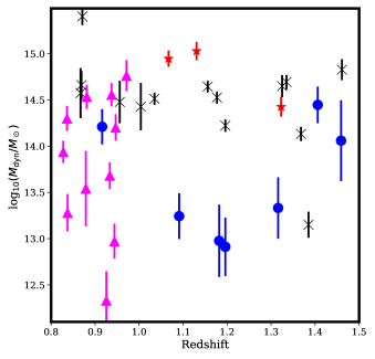
Figure 1 shows the velocity dispersions and redshifts of our sample. One cluster (COSMOS-125) is excluded, as a robust velocity dispersion could not be measured. Velocity dispersion calculations are described in § 4.2.3, and include redshifts from the literature. The three different selection classes are highlighted: SZ-selected (SPT), galaxy overdensity selected (SpARCS), and X-ray selected (COSMOS/SXDF). While these three selections were expected to correspond to very massive, typical, and low-mass clusters, respectively, in practice there is significant overlap between them. We also include the GEEC2 clusters (Balogh et al., 2014) on this figure; these fill in the low-dynamical mass region at $0.8<z<1$ . Here we estimate total dynamical masses from the velocity dispersion for all these systems using the simulation–derived scaling of Saro et al. (2013), and show these in the right panel (again omitting COSMOS-125). Dynamical masses span more than two orders of magnitude, from poor groups to very massive clusters.

Refer to caption — Figure 1: Left: The intrinsic velocity dispersion for each system in the GOGREEN and GCLASS samples is shown as a function of redshift. We also compare with the previously released GEEC2 sample (Balogh et al., 2014). Right: Velocity dispersions converted to dynamical mass estimates, based on the relation of Saro et al. (2013).

Name	RA	Dec	$z$	N_z	N_mem	$\sigma_{\rm int}$	References
	(J2000)					km/s	(Literature members)
SPT Clusters
SPT-CL J0546-5345	86.6562	-53.7580	1.068	63	34 (67)	$980\pm 70$	Sifón et al. (2016)
SPT-CL J2106-5844	316.5191	-58.7411	1.126	67	37 (50)	$1055\pm 85$	Foley et al. (2011)
SPT-CL J0205-5829	31.4390	-58.4829	1.323	65	24 (28)	$680\pm 60$	Stalder et al. (2013)
SpARCS Clusters
SpARCS0034-4307	8.6751	-43.1315	0.867	126	44	$700\pm 150$
SpARCS0036-4410	9.1875	-44.1805	0.869	114	48	$750\pm 90$
SpARCS1613+5649	243.3110	56.8250	0.871	152	94	$1350\pm 100$
SpARCS1047+5741	161.8890	57.6871	0.956	137	30	$660\pm 120$
SpARCS0215-0343	33.8500	-3.7256	1.004	110	48	$640\pm 130$
SpARCS1051+5818	162.7968	58.3009	1.034	176	42	$690\pm 40$
SpARCS1616+5545	244.1718	55.7571	1.157	195	60	$780\pm 40$
SpARCS1634+4021	248.6475	40.3643	1.177	176	69	$715\pm 40$
SpARCS1638+4038	249.7152	40.6452	1.194	161	56	$565\pm 30$
SpARCS0219-0531	34.9316	-5.5249	1.328	56	9	$810\pm 80$
SpARCS0035-4312	8.9571	-43.2068	1.335	121	29	$840\pm 50$
SpARCS0335-2929	53.7649	-29.4822	1.368	66	12 (27)	$540\pm 30$	J. Nantais (priv. comm)
SpARCS1034+5818	158.70560	58.3092	1.388	40	11	$250\pm 30$
SpARCS1033+5753	158.3565	57.8900	1.460	61	9	$955\pm 90$
COSMOS/SXDF Clusters							See § 4.2.3
SXDF64XGG	34.3319	-5.2067	0.916	17	1 (8)	$530\pm 80$
SXDF49XGG	34.4996	-5.0649	1.091	101¹	6 (14)	$255\pm 50$
COSMOS-63	150.3590	1.9352	1.1722	26	5 (8)	N/A
SXDF76bXGG	34.7474	-5.3235	1.182	80²	7	$210\pm 65$
COSMOS-221	150.5620	2.5031	1.196	54	9	$200\pm 50$
COSMOS-28	149.4692	1.6685	1.316	54	10	$285\pm 75$
COSMOS-125	150.6208	2.1675	1.404	39	7 (9)	N/A
SXDF87XGG	34.5360	-5.0630	1.406	101¹	8	$700\pm 110$
SXDF76aXGG	34.7461	-5.3041	1.459	80²	6	$520\pm 180$

•

¹ SXDF49XGG and SXDF87XGG share a single GMOS field. This number represents the total number of spectra in that field, so is the same for both groups.
•

² SXDF76aXGG and SXDF76bXGG share a single GMOS field. This number represents the total number of spectra in that field, so is the same for both groups.

Table 1: The table presents the 26 galaxy clusters and groups in the GOGREEN and GCLASS samples, ordered by redshift within three approximate halo mass classes. Redshifts are given in column (4), and the total number of GOGREEN and/or GCLASS spectra yielding good redshifts is given in column (5). The number of spectroscopically confirmed cluster members from GOGREEN and GCLASS combinedare shown in column (6). A following number in parentheses indicates the total number of members used to calculate the velocity dispersion, including values taken from the literature referenced in column (8). The intrinsic velocity dispersion of cluster members is given in column (7).

2.2 The GCLASS survey

The goal of GCLASS was to obtain at least ${\sim}50$ spectroscopic cluster members in each of ten clusters at $0.8<z<1.3$ , for the main purpose of understanding galaxy evolution in dense environments. To this end, priority was given to bright galaxies near the core of the cluster and close to the cluster red sequence in $z^{\prime}-[3.6\,\mu\mathrm{m}]$ colour. Nod-and-shuffle spectroscopy, combined with a strategy that used two offset GMOS pointings, allowed efficient sampling of the dense cluster cores as well as substantial radial coverage. For more details we refer the reader to Muzzin et al. (2012).

2.3 The GOGREEN survey

The GOGREEN survey is built upon a Gemini Large Program that ran from 2014 to 2019, using both telescopes over ten semesters to execute 432 hours of telescope time. Strong support from Gemini, through program extensions and Director’s Discretionary time, ensured that the project executed nearly 100 per cent of the originally allocated time (438h). The majority of this time was spent on multiobject spectroscopy; about 45h were used to obtain deep $z^{\prime}$ imaging with GMOS for target selection and mask design. Observations were acquired primarily in Priority Visitor mode, with the remainder executed in queue mode. Details of the observing runs are given in Appendix F.

Spectroscopic targets for the twelve SpARCS and SPT clusters were selected from deep IRAC and GMOS $z^{\prime}$ imaging, as described in Paper I. These were magnitude limited at $z^{\prime}<24.5$ and $[3.6\,\mu\mathrm{m}]<22.5$ , with broad, magnitude-dependent colour cuts to exclude galaxies at $z<0.7$ and $z>1.5$ (see § 5.1 for an illustration). For the nine clusters in COSMOS and SXDF, target selection was based on available³³3An unpublished, updated catalogue for SXDS was kindly provided by R. Quadri. photometric redshifts (Williams et al., 2009; Quadri et al., 2012; Muzzin et al., 2013).

Each cluster was observed with up to six slitmasks over the course of the survey, all centred at the same position and at the same position angle⁴⁴4The position angle is normally 90 degrees, to minimize atmospheric dispersion. However, guide star constraints often necessitated a different choice. In any case, the angle selected was independent of any feature of the target itself, including its orientation on the sky.. The faintest targets were observed on multiple masks, to increase the signal-to-noise of the spectrum. Existing data were examined when designing new masks, and objects were removed or reobserved in part based on the signal accumulated to that point. More detail about the mask design strategy is given in Paper I.

Imaging data were obtained through separate applications to multiple facilities following approval of the Large Program. While the minimum requirement for these data were to image the full GMOS field of view, most of the images cover a much wider field, allowing future, photometric studies of the environments surrounding these clusters out to many times the virial radius.

3 Observations and Data Reduction

3.1 Multiwavelength Imaging

3.1.1 Spitzer IRAC images

All SpARCS clusters have shallow ( $5$ - $\sigma$ depth of 7 $\mu$ Jy) imaging from the SWIRE survey (Lonsdale et al., 2003), from which the clusters were identified. Deeper channel 1 and 2 data ( $5$ - $\sigma$ depth in IRAC channel 1 of at least 2 $\mu$ Jy, or AB=23.1) exist for most of the clusters, from SERVS (Mauduit et al., 2012), S-COSMOS (Sanders et al., 2007), SpUDS (PI J. Dunlop, as described in Galametz et al., 2013) and GTO programs 40033 and 50161 (PI G. Fazio). The remaining clusters were observed as PI programs (PI Brodwin, from program ID 70053 and 60099 and McGee, program 13046). Some MIPS data from SWIRE and GTO programs 40033 and 50161 (PI G. Fazio) are available for the SpARCS clusters, but these are not used in the analysis nor included in this release.

There were small astrometric offsets (typically $\sim 1$ ″ between the stacks from these different programs. These were corrected with respect to the USNO-B1 catalogue (Monet et al., 2003), and all reduced data from different programs were stacked together. The stacks cover 10 $\arcmin$ on a side, with a pixel scale of 0.2 arcsec/pixel, and have an AB magnitude zeropoint of 21.58.

3.1.2 GMOS $z^{\prime}$ -band images

The deep GMOS imaging in $z^{\prime}$ obtained as part of GOGREEN is described in Paper I. The images were reduced by Gemini staff using their pipeline for producing mask-design preimages. These are scientifically useful, though not optimized for photometry of the faintest sources. The sky subtraction in particular is not optimal, as effects from bright sources remain in the sky frames, leading to non-Poisson noise in the background. However, for most systems we have wider field $z-$ band coverage from other facilities that supersedes the GMOS imaging (van der Burg et al., 2020).

GCLASS $z^{\prime}$ imaging was obtained from CTIO and CFHT, as described in Wilson et al. (2009), Muzzin et al. (2009) and Muzzin et al. (2012).

3.1.3 Ground-based optical and infrared imaging

A significant effort was undertaken to obtain deep imaging for all GOGREEN systems outside the COSMOS and SXDF fields. New and archival data were obtained from Subaru, VLT, Magellan, Blanco and CFHT, spanning the full observable optical/infrared wavelength range from $u$ to $K$ . These data and basic processing steps are described in van der Burg et al. (2020).

Near-infrared data were processed with custom pyraf scripts, based closely on the procedure described in Lidman et al. (2008). All images are astrometrically registered, to within $0\aas@@fstack{\prime\prime}1$ precision, to the USNO-B1 catalogue (Monet et al., 2003).

The Subaru Suprime-Cam data were processed at the CADC using a dedicated pipeline (Gwyn 2020, ASP Conference Series, in press). The archival raw images are detrended using SDFRed⁵⁵5https://www.subarutelescope.org/Observing/Instruments/SCam/sdfred/sdfred2.html.en, astrometrically calibrated using Gaia DR2 as a reference, and photometrically calibrated using Pan-STARRS photometry converted into the Suprime-Cam photometric system. Image defects (bad columns, cosmic rays) are masked and then the calibrated, detrended images are resampled and combined using SWarp⁶⁶6https://www.astromatic.net/software/swarp. The more recent, HypersuprimeCam data were fully processed using the hscPipe software⁷⁷7https://hsc.mtk.nao.ac.jp/pipedoc/pipedoc_6_e/ (v6.0).

For GOGREEN, the $J-$ and $K_{s}$ -band photometric zero points were calibrated with respect to 2MASS (Jarrett et al., 2000). Calibration of all the other filters was done based on the universality of the stellar locus (cf. High et al., 2009). Stellar spectra were obtained from the library of Pickles (1998), supplemented with Ivanov et al. (2004) in the near-infrared, and Kelly et al. (2014). These spectra were convolved with the response function for each telescope/filter combination used, and colour-colour diagrams were inspected to measure shifts relative to the stars identified in our own data (for examples, see Appendix A).

Colour measurements are based on aperture photometry performed on PSF-homogenised image stacks, constructed by convolving the individual stacks with kernels created with PSFEx (Bertin, 2011). For more details we refer to van der Burg et al. (2020). Image depths are reported in van der Burg et al. (2020), and calculated from the median 5 $\sigma$ limits within 2″ apertures measured on the PSF-homogenized images, corrected for Galactic extinction. Depths for most images are comparable to those of the UltraVISTA (McCracken et al., 2012; Muzzin et al., 2013) survey.

For GCLASS, optical $ugriz$ data for the northern clusters were obtained with MegaCam at CFHT. The southern clusters were imaged in $ugri$ with IMACS on Magellan, while the $z^{\prime}$ band imaging came from the MOSAIC-II camera on the Blanco telescope at CTIO. These data are described in van der Burg et al. (2013). Near-infrared imaging of the GCLASS systems from CFHT, Blanco and VLT are described in Lidman et al. (2012).

3.1.4 Hubble Space Telescope Imaging

New HST/WFC3 F160W imaging for the twelve GOGREEN clusters was obtained in a Cycle 25 program (GO-15294: PI Wilson). Each cluster was targeted with a $1\times 2$ mosaic of WFC3 pointings centered on the cluster, which covered a region of $136^{\prime\prime}\times 233^{\prime\prime}$ . At the redshift of GOGREEN clusters this corresponds to a $\sim 1.1\times 1.9$ Mpc rectangular region on the sky. Each pointing has 1-orbit depth. The orientation of the HST pointings (ORIENT) are constrained to within $20^{\circ}$ of the GMOS mask orientation to maximize the overlap between the imaging and the GOGREEN spectroscopic observations (see § 3.2.2 below for details).

The data are reduced and combined using Astrodrizzle (version 2.1.22, Gonzaga et al., 2012). The data reduction steps are described in Chan et al. (in prep). For the final drizzling, a pixel scale of $0\aas@@fstack{\prime\prime}06$ pixel^-1, a square kernel, and a pixfrac of 0.8 are adopted. Two sets of weight maps are produced using inverse variance map (IVM) and error map (ERR) weighting, respectively. The characteristic PSF of each cluster is constructed by median-stacking 5–22 bright, unsaturated stars. The full-width-half-maximum (FWHM) of the PSFs are $\sim 0\aas@@fstack{\prime\prime}17-0\aas@@fstack{\prime\prime}18$ .

We also provide the WFC3 F140W imaging obtained for the ten GCLASS clusters, described in Matharu et al. (2019). The pixel scale and pixfrac values are the same as for the F160W images, and the stellar FWHM is $\sim 0\aas@@fstack{\prime\prime}23$ .

3.2 Spectroscopy

3.2.1 GCLASS

The GCLASS spectroscopy is described in Muzzin et al. (2012). All the data were obtained with GMOS-S and GMOS-N, which cover a 5.5 $\times$ 5.5′ field of view. Slits were 1″ wide and 3″ long. With the R150 grating this results in a spectral resolution of $R=\lambda/\Delta\lambda_{\rm FWHM}=440$ (see § 3.2.2). Two overlapping pointings per cluster were used, so as to increase the coverage in the dense core of the clusters and somewhat extend the radial coverage beyond that of the GMOS field of view. Wavelength calibration was done exclusively using sky lines, following Abraham et al. (2004).

3.2.2 GOGREEN

A full log of the GOGREEN spectroscopic observations is given in Table LABEL:tab-specobs. Like GCLASS, spectroscopy was obtained with the GMOS-S and GMOS-N instruments, but with a single pointing per cluster. All observations on GMOS-S were obtained with the Hamamatsu detector array, which consists of three chips. Two of these have enhanced red response, while the chip at the blue end has enhanced blue response, relative to the older EEV detectors used for GCLASS. On GMOS-N, observations prior to 2017 were obtained with an array of EEV deep depletion detectors. In 2017, the GMOS-N detector was replaced with a Hamamatsu array identical to the one on GMOS-S.

GOGREEN used the same grating and slit size as GCLASS. We measure the spectral resolution for both surveys by fitting a Gaussian to the [O II] emission lines as described in Old et al. (2020, see § 4.2.2). We find $R=440\pm 60$ , or $\Delta\lambda_{\rm FWHM}\sim 19.3$ at $\lambda=8500$ Å.

The spectroscopic data reduction was based on the iraf⁸⁸8 ”IRAF is distributed by the National Optical Astronomy Observatories, which are operated by the Association of Universities for Research in Astronomy, Inc., under cooperative agreement with the National Science Foundation.” tools provided by Gemini, via the Ureka distribution. A variance (VAR) and data quality (DQ) plane were propagated through all the reduction steps. Wavelength calibration was done using CuAr arc lamps, usually taken after a night’s observing. At our low resolution, this lamp provides $\sim 10$ useful lines over the wavelength range $6200\,\mbox{\AA}<\lambda<10700$ Å. The typical rms of the wavelength solution is $\sim 0.5$ Å. All spectra (regardless of detector) are linearized and rebinned to 3.91 Å per pixel.

While GOGREEN used an order-sorting filter that blocked light bluer than 5150Å, in practice the wavelength calibration is not robust for $\lambda\lesssim 6000$ Å due to the lack of good arc lines at this resolution. To account for simple shifts in the zeropoint due to instrument flexure, we cross-correlate each sky spectrum with that of a reference slit, ideally chosen to have an accurate wavelength solution. The median shift for each mask is computed, and applied to the wavelength solution of that mask. Shifts are typically $<0.5$ pixels, though on occasion can be two or three times larger.

An important correction must be made for light that extends beyond the slit edges, an effect that is strongest at $\lambda>8500$ Å. This presents a problem for microshuffle nod-and-shuffle masks, where light from one spectrum contaminates the sky region of its shuffled counterpart, or other surrounding slits, in a way that does not subtract off. This effect was described by Abraham et al. (2004) and interpreted as charge diffusion. However, we observe the same effect using very different CCDs, and expect the origin is related to the instrument optics. A simple, average empirical model was developed in Abraham et al. (2004), to provide an average, approximate correction to all objects on a mask; this was applied to the GCLASS spectra. For GOGREEN the problem was acute, as we rely on the data at $>8500$ Å for redshift and absorption line studies at $z\gtrsim 1.2$ . We therefore developed a more sophisticated, empirical model for the effect. This model and its application to our data is described in Appendix B. We treat this as a form of scattered light, and refer to it as such throughout this paper. We fully reduce each mask, including wavelength calibration, sky subtraction and scattered light correction. All images of a given slit (sometimes taken on multiple nights or, rarely, even multiple semesters) are then median combined, rejecting the lowest and highest pixels. The one-dimensional (1D) spectra are extracted with a weighted Gaussian profile, as described in Paper I.

Telluric features in our spectra beyond $\lambda=9000$ Å are strong, and variable on short timescales. Initial attempts to correct for this absorption based on the baseline calibration of a single standard star taken each semester proved inadequate. We therefore derived a correction for each mask, using bright objects on the mask itself⁹⁹9This still is not ideal, as data for a given mask will have been obtained over several hours or even several nights. A frame-by-frame correction might do better, though without a dedicated bright star the signal would generally be too low for a good correction. In the end, this correction proves adequate for most of our data.. Midway through the project, when it was realized that a better procedure was needed, we added a single bright star to each mask for this purpose. As these stars were chosen to minimize impact on existing science slits they were not usually good telluric standards in the normal sense (they are often late-type stars), but they proved suitable for the procedure described in Appendix C. For masks where a star is not available we used either a bright galaxy spectrum, or a stacked spectrum of the 5–15 brightest objects.

The wavelength-dependent response of the observing system was calibrated using standard star observations, generally taken once per semester as part of Gemini baseline calibrations, not directly associated with this program. As described in Muzzin et al. (2012) and Balogh et al. (2017), we find that the shape of this response is stable over time, and we apply a single correction to all spectra (though separately for GCLASS and GOGREEN). We expect that this calibration is typically good to about 10 per cent, based on a comparison with SED templates fit to the photometry. An absolute flux calibration is determined where possible, by comparing to the available $i-$ band photometry as described in Appendix D. The main exception is for the spectra associated with SpARCS1033, for which K-band imaging (and, hence, photometric catalogues) are not yet available. Some galaxies with spectra do not have a match in the photometric catalogues because they lie in a masked region; no absolute calibration is applied in these cases.

4 Derived Data Products

4.1 Photometric Products

4.1.1 Photometric Redshifts, Stellar Masses and Rest-Frame Colours

Photometric redshifts for GOGREEN are determined using EAZY (Brammer et al., 2008, version May 2015), as described in van der Burg et al. (2020). Small residuals relative to the spectroscopic redshifts (see § 4.2.1) were corrected by fitting and applying a low order polynomial correction. These corrected redshifts are what are provided in the data release, and used throughout this paper.

Stellar masses and rest-frame colours are measured by fitting stellar population synthesis models of Bruzual & Charlot (2003) with the FAST (Kriek et al., 2009) code, assuming a Chabrier (2003) initial mass function. Details are again provided in van der Burg et al. (2020). These models assume simple star formation histories parametrised with a declining exponential function. This is known to underestimate the stellar mass by up to 0.3 dex compared with nonparametric (binned) star formation histories (Leja et al., 2019).

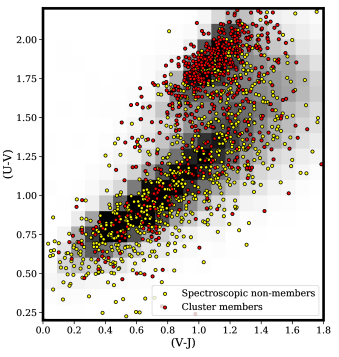
The rest-frame (U-V) and (V-J) colours are shown in Figure 2, for all galaxies in the GCLASS and GOGREEN samples with secure redshifts (see § 4.2.1) within $0.8<z<1.5$ . Galaxies identified as likely cluster members (see § 4.2.3) are shown in red. For comparison, the full photometric sample, including the Ultravista (Muzzin et al., 2013) and SPLASH (Mehta et al., 2018) catalogues¹⁰¹⁰10We compute UVJ colours for all galaxies in the SPLASH catalogue using the same procedure as for the clusters, and these are provided in the data release as described in § 6. For Ultravista, we use the UVJ colours in the catalogue, which were computed in the same way., is shown in greyscale. The bimodality of the colour distribution is evident, as is the dominance of the quiescent population among cluster members. We use these colours to define the quiescent galaxy population through this work, as

(\mathrm{U}-\mathrm{V})>1.3\,\,\cap\,\,(\mathrm{V}-\mathrm{J})<1.5\,\,\cap\,\,(\mathrm{U}-\mathrm{V})>0.88\,(\mathrm{V}-\mathrm{J})+0.59

(1)

as defined in Muzzin et al. (2013) for $1{<}z{<}4$ , adapted from Williams et al. (2009).

4.2 Spectroscopic Products

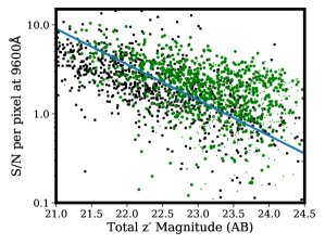
In Figure 3, we show the correlation between S/N per pixel in each final spectrum and the total $z^{\prime}$ -band magnitude of the galaxy. The S/N ratio here is the average S/N within $9500<\lambda<9700$ Å. There is significant scatter, reflecting the fact that spectra were obtained with a range of exposure times, detectors, and in a variety of conditions over several years. Some scatter is also likely caused by different galaxy sizes, which affect the amount of light going down the slits of fixed width. Notable is the flattening of the relation for GOGREEN spectra at magnitudes ${>}23.25$ , relative to the declining S/N that would be expected for fixed exposure time (solid line). This is because galaxies fainter than this magnitude are observed on multiple masks, to build up the total integration time. As a result, $\sim 80$ per cent of the spectra have $\mathrm{S/N}>1$ per pixel.

4.2.1 Redshifts

Spectroscopic redshifts for GCLASS were determined by comparison with templates within the iGDDS software (Abraham et al., 2004). For GOGREEN we used the Manual and Automatic Redshifting Software (marz, Hinton et al., 2016), with the default templates supplemented by stacked spectra of red and blue $z>1.5$ galaxies from GMASS (Kurk et al., 2013). Redshifts were determined interactively, using custom software to show the image, one- and two-dimensional spectra, and photometric redshift information (with 68 per cent confidence limits) for each galaxy in addition to the marz cross-correlation results. Quality flags are assigned based on a largely subjective assessment of the redshift likelihood, and considering the photometric redshift. These flags are described in § 6.4, and included in the data release as Redshift_Quality (see Table 4). The GCLASS redshift quality flags have been translated onto this system, so all spectra in this release have a uniform classification. We consider galaxies with Reshift_Quality $>2$ to be "good", and these are used in all the analysis here and in accompanying science papers, unless explicitly stated otherwise.

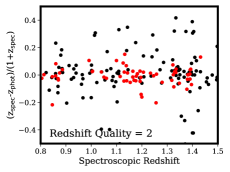
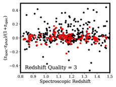
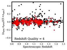
To quantify the accuracy and precision of the photometric redshifts, we compare these with the spectroscopic redshifts in Figure 4¹¹¹¹11Recall from § 4.1 that the photometric redshifts have had a small empirical correction applied to remove offsets relative to the spectroscopic redshifts.. For this comparison we consider only the subsample of galaxies with good quality spectroscopic redshifts in the range $0.8<z<1.5$ . Quiescent galaxies are indicated with red circles. Considering all galaxies with good spectroscopic redshifts (Redshift_Qualit $>2$ ), we find excellent agreement with the photometric redshifts, with an outlier fraction¹²¹²12Following van der Burg et al. (2020), we define outliers as those for which $|\Delta z|/(1+z)$ ¿0.15. of 7.3 per cent, and a standard deviation (after rejecting outliers) of $0.05$ in $\Delta z/(1+z)$ . Restricted to the quiescent galaxy subsample the standard deviation is similar, at 5.8 per cent, but the outlier fraction is much smaller, only 1.1 per cent. We use this as an indicator of our photometric redshift accuracy.

However, we also recognize that some of the outliers may be due to incorrect spectroscopic redshifts. We see in fact that the outlier fraction increases from 4.5 per cent for the quality class 4 galaxies, to 13 per cent for quality class 3, and 22 per cent for quality class 2 (which generally should not be used for science). The redshift quality flag is not independent of the photometric redshift, since good agreement with the latter is considered when assigning confidence to the spectroscopic redshift. It is therefore not possible from this analysis to robustly determine what fraction of spectroscopic redshifts might be incorrect, but it is likely $<10$ per cent of those with quality flag 3, and significantly more for those with quality flag 2.

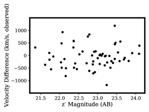
To assess the accuracy and precision of the GOGREEN spectroscopic redshifts, we compare the spectroscopic redshifts of the 61 objects with good redshifts in common with GCLASS. The observed-frame velocity difference of these spectra are shown in Figure 5, as a function of magnitude in the $z^{\prime}$ -band. Of these 61 objects, only one (not shown on the plot), is a significant outlier, with a velocity difference of $>1000$ km/s. The standard deviation of the rest of the sample is $393.5$ km/s, with no significant dependence on magnitude, redshift or S/N in the spectrum. Assuming GOGREEN and GCLASS have comparable, normally distributed redshift uncertainties, this means the typical uncertainty on an individual redshift is $278$ km/s. In the rest-frame of the clusters (all at $z>0.8$ ), this corresponds to an uncertainty of $<154$ km/s. There is also an unresolved bias, such that GOGREEN redshifts are smaller than those measured in GCLASS, by $95$ km/s (observed frame). As this is small relative to the typical uncertainty, and to the velocity dispersions of the clusters, we do not apply any correction. For the three SPT clusters, we have 22 GOGREEN redshifts that overlap with published redshifts in Stalder et al. (2013), Brodwin et al. (2010) and Foley et al. (2011). The median and standard deviation of the redshift difference is 25km/s and 550km/s, respectively, and there are no significant outliers.

About 15 per cent of the GOGREEN spectra obtained were severely compromised by a) contamination from bright, nearby objects; b) excess flux from the target or neighbours in the sky sampled region; c) poor sky subtraction or telluric correction; or d) large and critical regions of wavelength space affected by uncorrected scattered light or detector issues. We flag these spectra and exclude them from the redshift completeness statistics here. As there is no possibility to obtain a redshift from them, regardless of the intrinsic source characteristics, it is appropriate to treat them as if they were never observed.

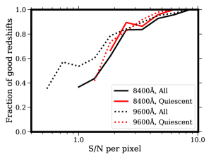
In Figure 6 we show the fraction of GOGREEN spectra for which we obtained a confident redshift, as a function of S/N per pixel. Only primary targets – those that satisfy our colour and magnitude selection boundaries – that are not flagged as described above are considered here. The S/N is considered at two different wavelengths — 8400Å and 9600Å — as shown. We obtain redshifts for about 50 per cent of these targets at S/N $\sim 1$ per pixel at 9600Å. The success rate is $>80$ per cent at $\mathrm{S/N}>2$ . For $\mathrm{S/N}>2$ , the success rate is independent of galaxy type. Lower S/N redshifts primarily come from emission line galaxies.

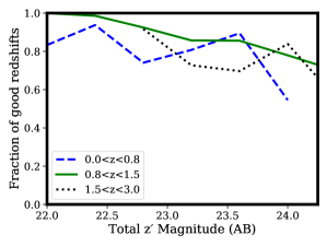
In Figure 7 we show how the GOGREEN redshift success rate depends on magnitude and the photometric redshift of the target. We only consider unflagged galaxies with $\mathrm{S/N}>1$ per pixel here. As expected, our redshift success rate is somewhat lower for galaxies with photometric redshifts $z<0.8$ or $z>1.5$ , for which our spectral range does not cover key spectral features. For galaxies in our target range of $0.8<z<1.5$ , the success rate is $>80$ per cent at all magnitudes. It is plausible that many of the galaxies for which we do not obtain a good redshift, especially at the faintest magnitudes, are actually at redshifts that lie well outside our targeted range despite what is indicated by their most probable photometric redshift.

4.2.2 Line Indices and [O II]-based star formation rates

Several spectroscopic indices are computed and provided as part of this data release. The [O II] $\lambda$ 3727 emission line was measured as described in Old et al. (2020). Briefly, a model consisting of a Gaussian component superposed on a linear continuum was fit to every spectrum, and compared with a continuum-only model. The Bayesian Information Criterion (BIC) is then used to identify objects for which the fit with the Gaussian component is preferred. Objects with $\Delta{\rm BIC}>10$ are likely to be secure detections, while those with $\Delta{\rm BIC}<10$ are likely secure non-detections. The catalogue provides equivalent widths and line fluxes, as well as the $\Delta{\rm BIC}$ value. The width of the Gaussian component is also left as a free parameter (as is the redshift, with a tight prior), and the values were used to determine the spectral resolution reported in § 3.2.

Star formation rates (SFRs) are estimated from the [O II] fluxes, using the calibration of Gilbank et al. (2010). This is a stellar-mass dependent calibration relative to H $\alpha$ -derived SFRs at $z=0$ . Because [O II] is strongly dependent on dust, ionization, and metallicity, there is significant scatter in this relation. It is therefore most useful for determining the average SFR of a population, rather than as an indicator for individual galaxies.

We also provide measurements of the 4000 Å break, and the equivalent widths of the [O II] emission and H $\delta$ absorption lines, following the definitions in Balogh et al. (1999). The D_n4000 index is an age-sensitive colour, based on the average value of $f_{\nu}$ in a narrow wavelength range on either side of the break. Individual measurements of H $\delta$ typically have large uncertainties, and should be used with caution. The [O II] equivalent widths are provided as an alternative to the Gaussian-modeling approach described above.

4.2.3 Cluster Velocity Dispersions and membership

Cluster members for GCLASS were selected based on a simple $\Delta v\leq 1500$ km/s criterion, as described in Muzzin et al. (2012). Velocity dispersions presented in Biviano et al. (2016) were determined using standard methods (e.g. Beers et al., 1990). As these clusters are generally very well defined in velocity space, these simple methods work adequately for most purposes.

For the clusters in GOGREEN, velocity dispersions are computed including all available redshifts from the literature. The total number of members used is reported in parentheses in column (6) of Table 1, with the references provided in the final column. The membership and velocity dispersion for the SPT and SpARCS clusters are derived as described in Biviano et al. (in prep). First, the main redshift peak is identified following Beers et al. (1991), and any significant substructure identified using the KMM algorithm (McLachlan & Basford, 1988). A small amount of substructure is only identified in two clusters (SpARCS1051 and SpARCS1616). Membership is then assigned based on their location in projected phase space. Two different algorithms are used. CLEAN (Mamon et al., 2013) is an established method, theoretically motivated based on the results of simulations. We also consider a new algorithm, CLUMPS, that is less model dependent. The difference in membership resulting from the two algorithms is small (usually within 10 per cent), and we defer the details Biviano et al. (in prep). The number of galaxies identified as a member by either method is what is listed in Table 1.

The COSMOS and SXDF systems in GOGREEN are more challenging because they have relatively few spectroscopic members, often without a well-defined central concentration. Furthermore, the location of the X-ray detection provides an important prior on the central location, though the centroid of the low X-ray fluxes are often uncertain, as well. We use an iterative clipping algorithm, again making use of all available public spectroscopy as well as that from GOGREEN, to measure the velocity dispersion. For COSMOS, the literature redshifts are drawn from a compilation provided by M. Salvato (priv comm). SXDF redshifts are taken from UDSz (Bradshaw et al., 2013; McLure et al., 2012), XMM-LSS (Melnyk et al., 2013; Chiappetti et al., 2013) and VANDELS (Pentericci et al., 2018). Cluster members are defined as those within $1$ Mpc and $2.5\sigma$ of the iteratively-determined spatial and velocity centre, respectively. In each iteration, the centre itself is the unweighted average position of those members within a 1 Mpc area centered on the X-ray detection. In some cases, there are many galaxies within the velocity dispersion of the cluster that lie outside the $1$ Mpc limit; in that sense, membership with the larger scale structure defining these systems can be larger than what is reported in Table 1. Uncertainties on the velocity dispersion are computed by bootstrapping the sample of selected cluster members. Full details will be available in Reeves et al. (in preparation).

5 Spectroscopic sample characteristics

The final spectroscopic catalogue for GCLASS and GOGREEN consists of $2771$ unique objects, of which $2257$ have good redshifts: $1529$ from GOGREEN, and $728$ from GCLASS¹³¹³13Where there is an observation from both surveys, we retain only the GOGREEN spectrum and redshift for the final catalogues and analysis.. An overview of our spectroscopic sample in the range $0.8<z<1.5$ is shown in Figure 8. All one-dimensional spectra with good redshifts, from both surveys, are displayed in order of redshift. Key emission and absorption features are clearly visible throughout the redshift range, as is the excellent quality of the sky subtraction at the red end of the spectra.

In Figure 9 we show the distribution in redshift and stellar mass, for most of the spectroscopic sample within $0.8<z<1.5$ ; SpARCS1033 is omitted from the plot since $K$ -band selected catalogues are not available at this time. Quiescent galaxies are indicated with red circles. The clustering in redshift space is readily apparent, and corresponds to the locations of the targeted systems, indicated with green triangles at the top of the Figure.

5.1 GOGREEN Completeness

We now consider how the spectroscopic completeness in GOGREEN depends on colour, magnitude, stellar mass, spectral type, and position. This can vary significantly from cluster to cluster. The geometric sampling in particular is non-trivial to characterize because the GOGREEN spectroscopy does not uniformly sample the area around the cluster, but is preferentially aligned along one (arbitrary) axis, perpendicular to the dispersion direction.

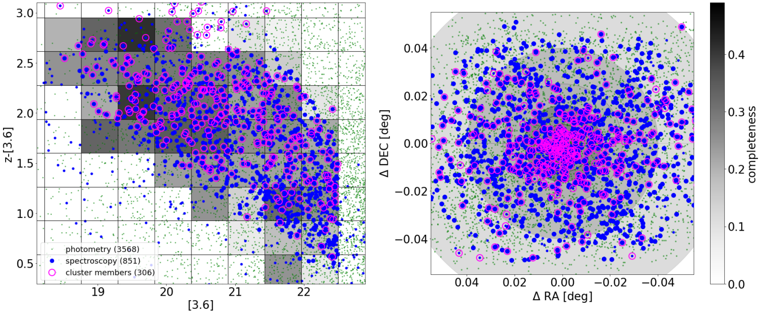
The completeness with respect to the observed colour and magnitude selection in GOGREEN is described in detail, and presented for the twelve SpARCS and SPT clusters included in the GOGREEN survey (including SpARCS1033, as the $K$ -band catalogues are not needed for this analysis), in Appendix E. Here we provide a summary of the average completeness for these twelve systems, in Figure 10. Targets were selected with primary limits [3.6 $\mu$ m]<22.5 and $z^{\prime}$ <24.25, with colour cuts to exclude foreground and background galaxies. While the blue cut is the same for all fields, the red selection limit was adjusted for each cluster, depending on its redshift. This defines the band within which most of our spectroscopy lies in the left panel of Figure 10; the few objects outside those bounds are "mask-filler" objects. The greyscale corresponds to the completeness within each colour-magnitude cell; overall, spectroscopic sampling within the colour boundaries is about 25 per cent, dropping somewhat with magnitude but not strongly dependent on colour. The panel on the right shows the spatial distribution of the spectroscopy for the same twelve clusters, with greyscale again representing completeness in broad radial bins. While there was no explicit geometric selection criteria in GOGREEN, the single GMOS pointing in each cluster effectively limits the spectroscopy to a broad stripe no more than 5′ in length.

For most analyses, what is likely to be most relevant is how complete the spectroscopic sample is relative to the population of likely cluster members, in terms of physical parameters like stellar mass, clustercentric distance and galaxy type. We can evaluate this using the photometric catalogues, available for all our systems except SpARCS1033. Here, we consider the parent cluster population to be all galaxies for which the cluster redshift lies within the 68 per cent confidence limits of the photometric redshift. We then count how many of those galaxies have a robust redshift, regardless of whether or not that redshift is consistent with that of the cluster. The ratio of these numbers is shown as the completeness in Figure 11, as a function of clustercentric distance and stellar mass. Above a mass of $\sim 10^{10.2}~{}\mathrm{M}_{\odot}$ , the completeness is more than 30 per cent, out to beyond 500 kpc from the cluster core. Most notably, the completeness for quiescent galaxies (classified from their rest-frame UVJ colours) above this mass limit is comparable to that of the sample as a whole. The drop in completeness at low stellar masses is partly driven by the fact that the 68th percentiles on the photometric redshift estimates get larger, so the parent sample to which we compare increases relative to the true underlying cluster population.

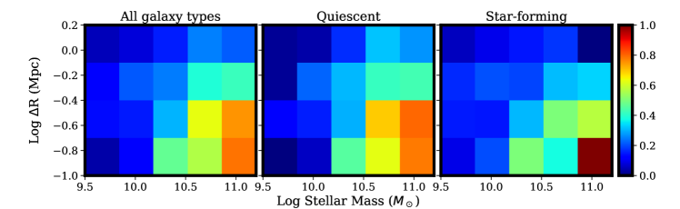
Based on this, we conclude that the spectroscopic catalogue provides a significant ( $\sim 45$ per cent on average) sampling of the parent cluster population within $500$ kpc, and for masses $>10^{10.2}~{}\mathrm{M}_{\odot}$ , that is not strongly biased with respect to galaxy type. An exception to this might be strongly dust-reddened (likely massive, star-forming) galaxies, which would be biased against during target selection and also when determining spectroscopic redshifts.

6 Public Data Release Contents

Here we describe a summary of the public data release contents. Three main catalogues are included in this publication, and available via linked online resources. These are the main cluster catalogue (§ 6.1); the redshift catalogue (§ 6.4); and a photometric catalogue with a subset of available information expected to be most commonly useful (§ 6.3). All catalogues, including the full $K_{s}$ -selected photometric catalogues, and reduced data (images and spectroscopy) are available via the CADC (https://www.cadc-ccda.hia-iha.nrc-cnrc.gc.ca/en/community/gogreen), and NSF’s NOIRLab (https://datalab.noao.edu/gogreendr1/). Pointers to these catalogues and other information can currently be found on the GOGREEN web page at http://gogreensurvey.ca/data-releases/data-packages/gogreen-and-gclass-first-data-release/.

We provide two jupyter python3 notebooks with the data release. The first, DR1_Notebook, provides examples for reading the data, displaying spectra and images, and reproducing many of the plots in this paper. The second, build_Table3, is the notebook used to construct Table 3 from the raw photometric and spectroscopic catalogues.

6.1 Cluster Catalogue

We provide a fits table clusters.fits with information about each cluster in the GOGREEN and GCLASS samples. Column names and descriptions are given in Table 2. This includes position, redshift and velocity dispersion measurements, as well as filenames for the corresponding images and photometric catalogues.

column	parameter name	description
1	cluster	Short name of each cluster.
2	fullname	Longer format cluster name
3	cluster_id	An integer which is used to identify the corresponding photometry. It is a unique number for each SpARCS and SPT cluster; it is 14 for all COSMOS clusters and 13 for those in the SXDF.
4-5	RA_Best, DEC_Best	Coordinates, in J2000 degrees, for the best estimate of the cluster centre. For the SPT and SpARCS clusters, this is the location of the BCG. For the COSMOS and SXDF clusters, it is the average position of members as described in §4.2.3.
6-7	RA_GMOS, DEC_GMOS	Coordinates, in J2000 degrees, for the centre of the GMOS spectroscopic observations (GOGREEN only).
8	PA_GMOS	Position angle, in degrees, for the GMOS spectroscopic observations (GOGREEN only).
9	Redshift	Best estimate of the cluster redshift, based on available spectroscopy, including publicly available spectra from other sources not included in this release.
10-11	vdisp, vdisp_err	Velocity dispersion and its uncertainty, in km/s, computed as described in §4.2.3.
12-17	gogreen_mN	Name of each GOGREEN GMOS mask, for N from 1 to 6, used to obtain spectra for this program.
18-22	gclass_mN	Name of each GCLASS GMOS mask, for N from 1 to 5, used to obtain spectra for this program.
23	Kphot_cat	Name of K-selected photometry catalogue
24	photoz_cat	Name of photometric redshift catalogue
25	stelmass_cat	Name of catalogue with stellar mass information
26-37	IMAGE_X	Name of image for filter X for SpARCS and SPT clusters.
38	Preimage	Name of the GMOS z-band image, or Subaru pseudo-image, used for mask design. Note the preimages were used for mask design but are not optimally reduced, specifically regarding sky subtraction and astrometry.

Table 2: A description of the contents of the clusters.fits table, which contains information relevant to each cluster system in the GCLASS and GOGREEN surveys.

6.2 Images

All GOGREEN images are resampled to $3000\times 3000$ pixels, projected onto the tangent plane with pixel scale $0.200$ ″/pix in the center ( $\sim 10\arcmin$ on a side). Images in all filters are aligned in x and y position to aide in performing matched aperture photometry. The five $z<1$ GCLASS clusters that are not part of GOGREEN are prepared in a similar manner, but are resampled to a pixel scale of $0.185$ ″/pix; furthermore the two northern clusters have a different size, of $5000\times 5000$ pixels.

For each cluster there are regular stacks, seeing-homogenised stacks (for aperture photometry), and (inverse-variance) weight maps. The seeing-homogenized stacks are convolved with a kernel to give them Moffat-shaped PSFs with Beta-parameter of 3.0, with FWHM in arcseconds listed in the file psfsize_target.dat. There is a second set of psf-homogenized images *psf2_*, for the $K_{s}$ -band and the IRAC images (with sizes in the file psfsize_target_psf2.dat) that are used to construct homogeneous $K$ -IRAC photometry as described in van der Burg et al. (2020).

Conservative, manual mask images are provided. These masks indicate pixels for which good data is available in all filters (excluding HST). As this mask requires the presence of IRAC data, which covers a relatively small field of view compared to the optical/NIR data, these pixel masks are conservative.

6.3 Photometry Catalogues

Each SPT and SpARCS cluster in the GOGREEN and GCLASS sample has an associated set of catalogues based on the multiwavelength imaging; the exception is SpARCS1033, for which deep $K$ -band imaging has not yet been obtained. These catalogues are all ascii format, and row-matched to the parent photometric catalogue. The detailed structure of these catalogues is described in the documentation distributed with the data release.

The parent catalogue, described in van der Burg et al. (2020), is constructed from the original (unconvolved) $K_{s}$ -band image as measured with SExtractor (Bertin & Arnouts, 1996). Each detected object is required to have five adjacent pixels with at least 1.5 sigma significance. All flux values have an AB magnitude zeropoint of 25 (equivalent to a flux scale of 0.3631 $\mu$ Jy per count). Therefore m_filter = $-2.5\times\mbox{log}_{10}(\mbox{flux\_filter})+25$ . An aggressive mask is applied, such that an object is unmasked (value totmask $=0$ ) only if data exists in all available bands (and for all sources in the SPLASH and UltraVISTA catalogues). It is therefore very conservative and might not be appropriate for some analyses. In particular, the IRAC data typically cover a limited area around the cluster; for science where IRAC coverage is not necessary, it can be appropriate to consider masked objects.

The COSMOS and SXDF photometry all comes from publicly available catalogues: Muzzin et al. (2013) and Mehta et al. (2018), respectively. These are not described in detail here. However, we provide jupyter notebooks for reading these data in a consistent way with our own catalogues.

For convenience, here we provide a single table photo.fits with some of the most useful parameters gathered from these catalogues, for all objects with photometric measurements in all available filters. The contents of this table are described in Table 3. The descriptions about how each parameter is computed apply to the SpARCS and SPT systems. For the COSMOS and SXDF, we use closely corresponding quantities from Muzzin et al. (2013) and Mehta et al. (2018), respectively. For SXDF we calculate the rest-frame $UVJ$ colours ourselves, using the EAZY code Brammer et al. (2008), as these are not provided in the Mehta et al. (2018) catalogue.

column	parameter name	description
1	Cluster	Name of the corresponding cluster, when there is an associated photometric catalogue. Objects in the COSMOS or SXDF photometric catalogues are identified with those labels, unless there is a GOGREEN spectroscopic redshift, in which case we use the name of the associated target. Note that SXDF49 and SXDF87 share a field, and are identified here only by SXDF49. Similarly SXDF76a and SXDF76b are identified here as SXDF76.
2	cPHOTID	This is a unique identifier for each object in this table. The first digit identifies the source of the photometry (1: GOGREEN; 2: GCLASS; 3: UltraVISTA/COSMOS; 4:SPLASH/SXDF). The next two digits are the cluster_id column from Table 2. The remaining numbers are the PHOTID identifier in the main photometric catalogues.
3	SPECID	The ID corresponding to Table 4 for objects with a corresponding GCLASS or GOGREEN spectrum.
4,5	ra,dec	J2000 positions, in degrees. Calibrated with SDSS DR7 or USNO-b whenever a cluster falls outside of the SDSS footprint.
6,7	zspec,Redshift_Quality	The spectroscopic redshift and quality flag for the associated spectrum, if any. Redshifts without a corresponding Redshift_Quality are copied from the parent (UltraVISTA or SPLASH) catalogue.
8,9,10	zphot,zphot_l68,zphot_u68	Photometric redshift, upper and lower uncertainties from the 68 per cent confidence region. Based on the zpeak output from EAZY (Brammer et al., 2008), where for the GOGREEN galaxies a polynomial correction is applied to improve the correspondence with spectroscopy.
11,12	$U{-}V$ , $V{-}J$	Rest-frame colours between Johnson $U$ , $V$ and $J$ , as measured with EAZY (Brammer et al., 2008). Small offsets, as described in van der Burg et al. (2020), have been applied on a cluster-by-cluster basis to improve correspondence with UltraVISTA. For the COSMOS galaxies the rest-frame colours are from the UltraVISTA catalogue.
13	Star	Star/galaxy classification based on colours, as described in van der Burg et al. (2020). Flag is 1 for a star, and 0 otherwise.
14	K_flag	SExtractor flag in the $K$ -band.
15	totmask	Manual mask at position of detection, where objects are masked (totmask $=1$ ) if they do not have an image in all available filters for that cluster. Only sources with totmask=0 are included in this compilation catalogue. Photometry for other sources must be obtained from the original catalogues.
16	Mstellar	Total stellar masses, measured with the FAST (Kriek et al., 2009) code and assuming the best redshift for the object (spectroscopic or zphot). These assume $\tau-$ model star formation histories, and are known to underestimate the stellar mass obtained with a non-parametric star formation history, by up to 0.3 dex (Leja et al., 2019). For objects in COSMOS and SXDF the stellar masses are taken from their respective catalogues.
17-46	$X_{i}$ _tot	Total fluxes in each filter $X_{i}$ . These are derived from the Ks_tot flux and the appropriate colour, computed in 2″ diameter circular apertures from PSF-matched images. IRAC aperture fluxes have been measured in a two-step process, similar to the description in Appendix A of van der Burg et al. (2013). The measurements within a 3″ aperture are scaled by a factor determined by comparing the 2″ aperture $K_{s}$ flux with that within a 3″ aperture measured on an image convolved to match the IRAC point spread function. This is done to avoid having to convolve all the high resolution ground-based data to the IRAC psf. For objects in COSMOS and SXDF the fluxes are taken from their respective catalogues, scaled by the corresponding Ks_tot flux. Includes: $u,g,r,i,z,y,V,B,J,H,K_{s},\mathrm{IRAC1},\mathrm{IRAC2},\mathrm{IRAC3},\mathrm{IRAC4},\mathrm{IA}484,\mathrm{IA}527,\mathrm{IA}624,\mathrm{IA}679,\mathrm{IA}738,$ $\mathrm{IA}767,\mathrm{IB}427,\mathrm{IB}464,\mathrm{IB}505,\mathrm{IB}574,\mathrm{IB}709,\mathrm{IB}827,{fuv},{nuv}$ , and ${mips24}$ .
47-77	e $X_{i}$ _tot	Associated uncertainty estimates for filter $X_{i}$ , assuming that the sole source of uncertainty is the background rms. It therefore depends on position on the stack (as the depth is not necessarily uniform), but does not depend on the source flux.

Table 3: A description of the contents of the photo.fits table, which contains selected photometric data for each cluster system in the GCLASS, GOGREEN samples, COMOS UltraVISTA (v1.4; Muzzin et al., 2013) and SXDF SPLASH(v1.6; Mehta et al., 2018) fields.

6.4 Redshift Catalogue

The redshift catalogue Redshift_catalogue.fits, described in Table 4, includes an entry for every object with a GOGREEN or GCLASS spectrum¹⁴¹⁴14This excludes the stars deliberately observed on some masks for the purposes of telluric corrections.. There are no duplicates: if a galaxy has a spectrum in both surveys, only the GOGREEN entry is included here.

column	parameter name	description
1	Cluster	Short name of each cluster; matches the entry in Table 2
2	SPECID	A unique identification number. The first digit identifies the origin of the spectrum: 1 for GOGREEN and 2 for GCLASS. The next two digits correspond to the cluster_id identifier in the Cluster catalogue, that specify the photometric field. The remaining digits are the galaxy ID (only unique for a given field and source).
3,4	RA(J2000), DEC(J2000)	Target coordinates, in J2000 degrees. For GOGREEN, these coordinates correspond to the $z^{\prime}$ image coordinates used for mask design. These have been transformed to align with the $K_{s}$ images; however positions will not match exactly with coordinates in the photometric catalogues.
5	OBJClass	This has a value of 1 for GOGREEN primary targets, i.e. those that match our photometric selection criteria. A value of 3 corresponds to a GOGREEN "mask filler" object, and 4 identifies a GCLASS spectrum. (OBJClass=2 was reserved for stellar sources used for telluric correction, and these are not included in the catalogue).
6	Redshift	The redshift measured from the spectrum
7	Redshift_Quality	The redshift quality flag. Both quality 3 and 4 are secure galaxy redshifts and can be used for scientific analysis; the difference between them is subjective and not rigorously defined. Quality 2 is a "best guess" but should be used with caution; this includes cases where there is plausible consistency with the photometric redshift, but no clearly identifiable spectral features. Quality 1 means no redshift is available.
8	EXTVER	This is the science extension number in the fits files with the 1D and 2D spectra (see § 6.5).
9	Spec_Flag	An integer used to identify spectra that have problems that might compromise the ability to measure a redshift or line indices of a spectrum. Flags are assigned for the following: 1: Mild slit contamination or artefacts that should not strongly affect measurements 2: Non-galaxy-like spectrum and/or image 4: Significant slit contamination from neighbouring objects. Redshift and features may be compromised. 8: Poor telluric correction or sky subtraction, due for example to inadequate correction for the stray light effect described in Appendix B. 16: Major artefacts or large masked regions that render the spectrum nearly useless. Flags can be added. So, for example, a flag of 12 means there is both contamination from neighbouring objects, and poor sky subtraction.
10	SNR_8500_VAR	The signal-to-noise ratio per pixel, measured in the range $7500<\lambda<9500$ Å. The noise estimate is taken from the VAR array associated with the spectrum.
11	SNR_8500_RMS	The signal-to-noise ratio per pixel, measured in the range $7500<\lambda<9500$ Å. The noise estimate is taken from the rms in the science spectrum over the same range.
12,13	D4000, eD4000	The D_n4000 index as defined in Balogh et al. (1999), and its uncertainty. See § 4.2.2
14,15	EWOII, eEWOII	The equivalent width of the [Oii] emission line and its uncertainty, in Å, using the line index definitions in Balogh et al. (1999). Positive values represent emission. See § 4.2.2
16,17	EWHdelta, eEWHdelta	The equivalent width of the H $\delta$ absorption line and its uncertainty, in Å, using the line index definitions in Balogh et al. (1999). Positive values represent absorption. See § 4.2.2
18,19	EWOII_model, eEWOII_model	The equivalent width of the [Oii] emission line and its uncertainty, in Å, calculated from the Gaussian fitting model described in Old et al. (2020).
20,21	F_OII,eF_OII	The integrated flux of the [Oii] emission line and its uncertainty, in ergs/s/cm²/Å, calculated from the Gaussian fitting model described in Old et al. (2020).
22,23	SFR,eSFR	The star formation rate in solar masses per year, estimated from the [Oii] emission line flux and the stellar mass, using the calibration of Gilbank et al. (2010).
24	delta_BIC	The difference in Bayesian Information Criterion used to identify the presence of [Oii] emission ( $\Delta{\rm BIC}>10$ ) or its absence ( $\Delta{\rm BIC}<-10$ ). See Old et al. (2020) for more details.
25	member_Clean	Applicable only to the 11 SPT and SpARCS clusters in GOGREEN, this indicates likely cluster membership based on the clean algorithm of Mamon et al. (2013). A value of 1 indicates a member, 0 is a non-member, and -1 indicates membership could not be determined.
26	member_EM	Applicable only to the 11 SPT and SpARCS clusters in GOGREEN, this indicates likely cluster membership based on the C.L.U.M.P.S. algorithm of Munari et al. (in prep). A value of 1 indicates a member, 0 is a non-member, and -1 indicates membership could not be determined.
27	member	A flag that identifies likely cluster members (1) or nonmembers (0). A value of $-1$ means membership could not be determined. For SpARCS and SPT clusters in GOGREEN, this is the maximum of the member_Clean and member_EM flags. For the five GCLASS clusters we use the membership given in Muzzin et al. (2012). Finally, for the systems in COSMOS and SXDF we define members as those within 1 Mpc and 2.5 $\sigma$ of the centre, as described in § 4.2.3.

Table 4: A description of the contents of the spectroscopic redshift catalogue Redshift_catalogue.fits, which contains and entry for every unique object with a GOGREEN or GCLASS spectrum.

6.5 1D and 2D reduced spectra

Each cluster has an associated multi-extension fits file containing the final 1D spectra, and another with the 2D spectra, for every target. Each object has up to three entries, labeled sci for the science spectrum, var for its estimated variance, and, for GOGREEN spectra only, dq for a data quality flag. The science spectrum for object $i$ , for example, is accessed with the extension [SCI,i]. All spectra are 974 pixels long, with a linear dispersion of 3.906 Å per pixel, and starting at 6398.44 Å. This information is provided in the header of each extension. The header also includes keywords ’ORIG1’, ’ORIG2’ etc. containing the mask names and extensions of the spectra that were combined to make this final stack. The associated var array contains a first-principles estimate of the uncertainty on each pixel, as propagated through the data reduction pipeline. This includes a systematic term: during extraction, if the positive and negative version of the same wavelength pixel in the spectrum differ by more than five times the square root of the estimated variance, that difference is added in quadrature to the variance. The data quality (dq) array (only present for GOGREEN spectra) is likely of limited use; it corresponds to the number of pixels that were combined (along a CCD column) during the 1D extraction. Pixels and wavelength ranges that are flagged as bad¹⁵¹⁵15These wavelength ranges are also identified in the header as userbad. during the reduction or extraction process are excluded. Thus, large numbers ( $>10)$ represent good regions of the spectrum where most of the pixels in the slit were used; lower values mean only part of the slit was used. The latter happens most frequently when there is a neighbouring object contaminating the slit in one of the nod positions.

The GCLASS spectra were extracted differently from GOGREEN, and do not have a comparable var array. We construct a similar array from the science and sky spectra provided and scale it so that, on average, the relation between var and the rms of the science spectrum is the same as for GOGREEN.

The 1D fits file also contains an extension, labeled [MDF], which contains a binary table. This table is derived from the mask definition file (hence the extension name), and includes the position and magnitude of the spectrum corresponding to each extension. These and the other columns in this table are described in 5.

column	parameter name	description
1	ID	Corresponds to SPECID in Table 4
2	EXTVER	The extension number of each spectrum within this file.
3,4	RA, DEC	J2000 coordinates, in degrees, as in Table 4.
5	MAG	Total magnitude in the $z^{\prime}$ -band, from the preimages, used for target selection. This should generally not be used; magnitudes in the $K$ -selected photometric catalogues are better.
6	priority	This is the same as OBJClass in Table 4
7	qop	This is the same as Redshift_Quality in Table 4
8,9	SNR_8500_VAR, SNR_8500_RMS	These are the same as the entries in Table 4
10	Etime	Total exposure time, in seconds.

Table 5: A description of the contents of the MDF table extension associated with each 1D spectrum.

The 2D spectra are provided in another MEF fits file. The format is similar to the 1D file, but only GOGREEN spectra are included, so there are fewer extensions. There is no corresponding binary table extension in this file. Every spectrum is 974 pixels long and either 19 or 21 pixels wide. The dispersion axis is the same as for the 1D file; the spatial axis is in pixel units. No relative or absolute flux calibration is applied to these spectra.

7 Conclusions

We have presented the first public Data Release of the GCLASS (Muzzin et al., 2012) and GOGREEN (Balogh et al., 2017) galaxy cluster surveys. The main characteristics of the data sample are:

•

26 clusters spanning the redshift range $0.8<z<1.5$ , with dynamical halo masses spanning a wide range from the "massive group" scale of $\sim 10^{13}~{}{\rm M}_{\odot}$ to the most massive clusters at these redshifts, $\sim 10^{15}~{}{\rm M}_{\odot}$ .
•

Homogeneous, $K_{s}$ -selected photometric catalogues are available for all systems except SpARCS1033; these include PSF-matched photometry covering the full optical and near-infrared spectrum, at depths comparable to those of the UltraVISTA (Muzzin et al., 2013) survey.
•

Modest resolution ( $R=440$ ) Gemini GMOS spectroscopy has been obtained covering the full virialized region of each cluster. The redshift catalogue is $\gtrsim 30$ per cent complete and unbiased relative to spectral type for stellar masses $M_{\ast}\gtrsim 10^{10.2}~{}{\rm M}_{\odot}$ , within $\sim 500$ kpc of the centre.
•

The spectroscopic catalogue includes 2257 galaxies with good redshifts (Redshift_Quality $>2$ ), including nearly 800 cluster members.
•

Reduced HST/WFC3 imaging is provided in the F160W (GOGREEN) and F140W (GCLASS) filters; the five clusters that overlap these surveys have images in both filters. We also provide reduced archival ACS/F606W and ACS/F814W images for the three SPT clusters in GOGREEN.

This data release includes all reduced images and spectroscopy. It represents hundreds of hours of 8-m class and space-based observations, dedicated to a comprehensive and homogeneous survey of dense galaxy systems that are rare in blank field surveys at this depth. Catalogues of advanced data products including photometric and spectroscopic redshifts, rest-frame colours, stellar masses, spectral line indices and cluster membership are also provided. The tabular data for most commonly used quantities are included in the tables within this paper. Future releases, science results and other updates will be announced via the GOGREEN website at http://gogreensurvey.ca/.

Data Availability

Access to the GOGREEN and GCLASS data release, including jupyter python3 notebooks for reading and using the data, is available at the CADC (https://www.cadc-ccda.hia-iha.nrc-cnrc.gc.ca/en/community/gogreen), and NSF’s NOIRLab (https://datalab.noao.edu/gogreendr1/). Future releases, science results and other updates will be announced via the GOGREEN website at http://gogreensurvey.ca/.

Acknowledgments

This work was enabled by observations made from the Gemini North, Subaru and CFHT telescopes, located within the Maunakea Science Reserve and adjacent to the summit of Maunakea. We are grateful for the privilege of observing the Universe from a place that is unique in both its astronomical quality and its cultural significance.

We extend our thanks and appreciation to Gemini, and the Gemini communities, for supporting this Large Program. The extension of the program from the original allocation of 3 years and 438 hours to the final, 5 years and 530 hours needed to complete the survey was critical for achieving our science goals. Queue mode observations, and a small amount of Director’s Discretionary time, was used to make up for time lost during Priority Visitor runs, ensuring the survey finished at nearly 100 per cent completeness. We also thank Gemini for their financial support of junior observers on several of our observing runs.

The authors would like to acknowledge research grant funding that has enabled this research, including: NSERC Discovery grants (MLB and AM) and CGS-D (KW); National Science Foundation grants AST-1517815, AST-1517863 (GW), AST-1716690, and AST-1814159 (GHR), AST-1518257 and AST-1815475 (MC); NASA HST program grants GO-15294 (GW), AR-14289 (MC) and AR-14310 (GHR); by grant numbers 80NSSC17K0019 (GW) and 80NSSC19K0592 (GR) issued through the NASA Astrophysics Data Analysis Program (ADAP), PRIN MIUR 2017 n.20173ML3WW_001 (PI Cimatti) and the INAF main-stream funding programme (BV); the Chilean Centro de Excelencia en Astrofísica y Tecnologías Afines (CATA) BASAL grant AFB-170002 (RD). G.R. also acknowledges the support of an ESO visiting science fellowship.

This paper includes data gathered with the Gemini Observatory, which is operated by the Association of Universities for Research in Astronomy, Inc., under a cooperative agreement with the NSF on behalf of the Gemini partnership: the National Science Foundation (United States), the National Research Council (Canada), CONICYT (Chile), Ministerio de Ciencia, Tecnología e Innovación Productiva (Argentina), and Ministério da Ciência, Tecnologia e Inovação (Brazil); the 6.5 meter Magellan Telescopes located at Las Campanas Observatory, Chile, under programme IDs CN2015A-31, CN2016B-44, and CN2018B-14; the Canada-France-Hawaii Telescope (CFHT) which is operated by the National Research Council of Canada, the Institut National des Sciences de l’Univers of the Centre National de la Recherche Scientifique of France, and the University of Hawaii; MegaPrime/MegaCam, a joint project of CFHT and CEA/DAPNIA; Subaru Telescope, which is operated by the National Astronomical Observatory of Japan; the ESO Telescopes at the La Silla Paranal Observatory under programme IDs 097.A-0734 and 179.A-2005. We make use of data products produced by CALET and the Cambridge Astronomy Survey Unit on behalf of the UltraVISTA consortium. Finally, this research has made use of the SVO Filter Profile Service (http://svo2.cab.inta-csic.es/theory/fps/) supported by the Spanish MINECO through grant AYA2017-84089.

Affiliations

¹Department of Physics and Astronomy, University of Waterloo, Waterloo, Ontario, N2L 3G1, Canada
²Waterloo Centre for Astrophysics, University of Waterloo, Waterloo, Ontario, N2L 3G1, Canada
³European Southern Observatory, Karl-Schwarzschild-Str. 2, 85748, Garching, Germany
⁴Department of Physics and Astronomy, York University, 4700 Keele Street, Toronto, Ontario, ON MJ3 1P3, Canada
⁵Department of Physics and Astronomy, The University of Kansas, Malott room 1082, 1251 Wescoe Hall Drive, Lawrence, KS 66045, USA
⁶Department of Physics and Astronomy, University of California Riverside, 900 University Avenue, Riverside, CA 92521, USA
⁷INAF-Osservatorio Astronomico di Trieste, via G. B. Tiepolo 11, 34143, Trieste, Italy
⁸IFPU - Institute for Fundamental Physics of the Universe, via Beirut 2, 34014 Trieste, Italy
⁹Departamento de Ingeniería Informática y Ciencias de la Computación, Universidad de Concepción, Concepción, Chile
¹⁰Department of Physics and Astronomy, University of California, Irvine, 4129 Frederick Reines Hall, Irvine, CA 92697, USA
¹¹South African Astronomical Observatory, PO Box 9, Observatory, 7935, South Africa
¹²Centre for Space Research, North-West University, Potchefstroom 2520, South Africa
¹³Canadian Astronomy Data Centre, NRC Herzberg, 5071 West Saanich Road, Victoria, BC, V9E 2E7, Canada
¹⁴Research School of Astronomy and Astrophysics, The Australian National University, ACT 2601, Australia
¹⁵ Centre for Gravitational Astrophysics, College of Science, The Australian National University, ACT 2601, Australia
¹⁶Department of Physics and Astronomy, Texas A&M University, College Station, TX, 77843-4242, USA
¹⁷George P. and Cynthia Woods Mitchell Institute for Fundamental Physics and Astronomy, Texas A&M University, College Station, TX, 77843-4242, USA
¹⁸School of Physics and Astronomy, University of Birmingham, Edgbaston, Birmingham B15 2TT, England
¹⁹European Space Agency (ESA), European Space Astronomy Centre, Villanueva de la Cañada, E-28691 Madrid, Spain
²⁰Department of Astronomy and Astrophysics, University of Toronto 50 St. George Street, Toronto, Ontario, M5S 3H4, Canada
²¹Department of Physics, McGill University, 3600 rue University, Montréal, Québec, H3P 1T3, Canada
²²INAF - Osservatorio astronomico di Padova, Vicolo Osservatorio 5, IT-35122 Padova, Italy
²³Observatorio Astronómico de Córdoba (UNC) and Instituto de Astronomía Teórica y Experimetal (CONICET-UNC). Córdoba, Argentina.
²⁴University of California at Santa Cruz, 1156 High Street, Santa Cruz, CA 95064, USA
²⁵Department of Astronomy, University of Washington, Box 351580, U.W., Seattle, WA 98195, USA
²⁶Department of Physics, University of Helsinki, Gustaf Hällströmin katu 2a, FI-00014 Helsinki, Finland
²⁷Laboratoire d’astrophysique, École Polytechnique Fédérale de Lausanne (EPFL), 1290 Sauverny, Switzerland
²⁸Departamento de Ciencias Físicas, Universidad Andres Bello, Fernandez Concha 700, Las Condes 7591538, Santiago, Región Metropolitana, Chile
²⁹School of Earth and Space Exploration, Arizona State University, Tempe, AZ, 85287, USA
³⁰Department of Physics and Astronomy, McMaster University, Hamilton ON L8S 4M1, Canada
³¹Steward Observatory and Department of Astronomy, University of Arizona, Tucson, AZ, 85721

Appendix A Photometric calibration

As described in Sect. 3.1.3, the multi-band photometry is calibrated with respect to the universal stellar locus. In Fig. 12, we show the stellar locus for several different filter combinations. We note that the stars from the different clusters that are shown here, are selected based on their $u-J$ (or $g-J$ ) and $J-K_{\mathrm{s}}$ colours (as in van der Burg et al., 2020). In contrast, the photometric calibration was originally done on stellar candidates selected by their magnitude and size (unresolved objects) as measured with SExtractor.

The reference stellar spectral library from Kelly et al. (2014) is primarily based on SDSS spectroscopy, which covers the wavelength range 4100Å-9000Å. It is extended both in the red and blue by matching with similar objects in the Pickles (1998) library, where similarity is judged based on the region where there is wavelength overlap between both samples. Some sources in the Pickles (1998) library are matched to multiple SDSS sources, which leads to a “step-like” pattern in Fig. 12 in the Near-IR.

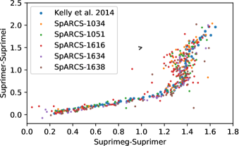
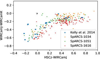
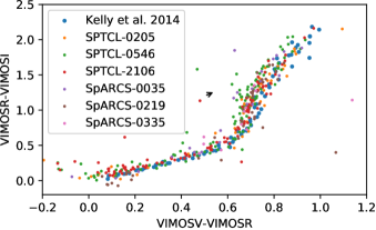
As one test to look for significant photometric calibration systematics in one particular filter, we look for residuals relative to the best-fit EAZY templates used to calculate photometric redshifts § 4.1. Consistently large residuals in one band could indicate a calibration error.

Specifically, we calculate $\sigma$ = $\frac{f_{observed}-f_{model}}{err_{observed}}$ for each filter used in the EAZY photometric fitting for each galaxy with a spectroscopic redshift. Then in each filter/cluster combination, we find the median residual across the entire redshift range spanned by the cluster’s spectroscopic catalogue. This includes both cluster members and field galaxies observed near the cluster, in an attempt to find any systematic effect as a function of redshift. We list our residuals in Tables 6 & 7 for northern and southern cluster respectively. We find that fits of all filter and cluster combinations are within 3 $\sigma$ of the observed data, with the highest residuals residing at the blue end of the SED fits. It is not trivial to identify the underlying cause of these residuals, which in any case are small. As one, illustrative test, we systematically increase the Suprime $g$ -band input magnitudes by the median residual measured for the northern sample, and rerun EAZY. No significant change is observed in the resulting residuals, relative to the new fits. While this rules out a simple zeropoint shift in this one filter as the cause of the systematic, the actual cause remains unknown and may still be related to the photometric calibration.

	SpARCS1034	SpARCS1051	SpARCS1616	SpARCS1634	SpARCS1638
MegaCamu		0.525	0.503	1.056	0.813
Suprimeg	1.400	-1.373	-1.892	-1.805	-2.327
Suprimer	-0.824	0.783	0.926	0.407	0.632
Suprimei	0.739	0.871	0.923	1.094	1.563
Suprimey					-1.163
HSCz	0.443	-0.086	-0.047
HSCy	0.384	0.299	-0.565
GMOSz				0.196	0.409
WIRCamJ	-0.861	0.007	-0.46509	-1.007	-0.424
WIRCamK	-0.376	-0.608	0.63699	0.201	-0.032
IRAC1	-0.970	-0.413	-0.58884	-0.797	-0.328
IRAC2	-0.511	-0.331	-0.26533	-0.364	-0.307
IRAC3	-0.054	-0.013	-0.04943	-0.063	-0.100
IRAC4	0.233	-0.025	0.09243	0.091	0.166

Table 6: Residual (

\sigma

\frac{f_{observed}-f_{model}}{err_{observed}}

) between input photometry of a given band and the modelled band flux using the EAZY best-fit template for northern clusters. Negative values indicate an overestimation during fitting and positive values indicate an underestimation.

	SPTCL0205	SPTCL0546	SPTCL2106	SpARCS0035	SpARCS0219	SpARCS0335
VIMOSU	1.702	2.046	1.451	2.326	1.082	2.043
VIMOSB	-0.796	-0.100	-0.413	-0.681	-0.814	-0.507
VIMOSV	0.121	-0.368	-0.028	0.157	0.051	0.32
VIMOSR	0.229	-0.062	0.075	0.217	-0.007	-0.294
VIMOSI	0.275	0.061	-0.447	0.197	0.762	0.078
VIMOSz	0.672	0.517	0.285		1.095	0.805
DECamz				0.093
HAWKIJ				0.243
HAWKIKs			0.284	-1.216
HAWKIY						0.047
FOURSTARJ1	-0.372	-0.074	-0.089	0.060	-0.103
FOURSTARJ	-0.836	-0.515	0.004		-1.273	-1.218
FOURSTARKs	-0.350	-0.003			-0.863	0.808
IRAC1	-0.881	-1.098	-0.754	-1.122	-0.476	-1.062
IRAC2	-0.412	-0.214	-1.286	-0.063	-0.319	-0.062
IRAC3				-0.047	0.033	-0.397
IRAC4				0.647	0.576	0.469

Table 7: Residual (

\sigma

\frac{f_{observed}-f_{model}}{err_{observed}}

) between input photometry of a given band and the modelled band flux using the EAZY best-fit template for southern clusters. Negative values indicate an overestimation during fitting and positive values indicate an underestimation.

Appendix B Correction for spectral contamination due to scattered light from nearby slits

The standard data reduction steps resulted in spectra that were unusable beyond about 9000Å, as the nod-and-shuffle background subtraction was failing to correctly remove the sky. This was traced to a wavelength-dependent effect, where the amount of light extending beyond the slit edge increases with increasing wavelength. This is catastrophic when slits are close together, as is the case for pairs of spectra taken in microshuffle mode, where the spectra from the two nod positions are adjacent to one another on the detector. An example is given in the left panels of Figure 13, which shows a region on the detector with five slits, at high stretch. Light extends far beyond the slit edge, particularly noticeable at the location of bright sky lines. This in particular blurs the distinction between the nod-and-shuffle pairs.

The same effect was noted by Abraham et al. (2004), and attributed to charge diffusion in the detector. However, we find the effect is quantitatively similar for detectors used through the course of this project that have very different sized depletion zones, which makes this explanation unlikely. We considered scattering from the grating (e.g. Woods et al., 1994; Ellis et al., 2014), but a quantitatively similar effect is seen in the undispersed through-mask images. The origin remains unknown, therefore, but seems to be an optical effect independent of the grating and detector.

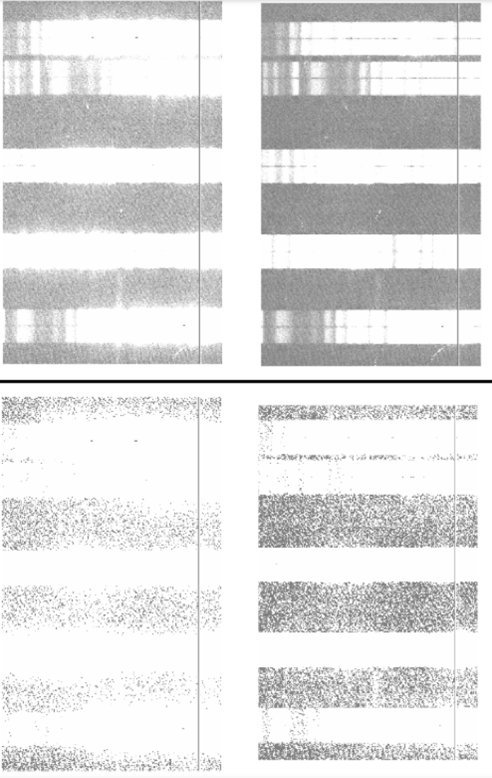
In Balogh et al. (2017) we described a procedure for empirically correcting the effect. However, this method was only applicable to nod-and-shuffle pairs of spectra that are of a fixed separation and aligned in wavelength. Because of our high slit density, there are many other examples where light from a nearby slit contaminates another; an example is the two slits at the top of Figure 13. As the amount of contamination is sensitive to wavelength and distance from the slit edge, this is more difficult to correct for.

Our approach is to build an empirical model that describes the amount of flux that "leaks" outside a slit, relative to the average intensity within the slit, as a function of wavelength, distance from the slit edge, and intensity. This is made possible because we have so many different masks, obtained with nearly identical setup (same grism, slit length and nod parameters). We are able to select a subset of slits which, over some wavelength range, are well separated from any other slit on the mask. We then simply measure the amount of signal in the region outside the slit. By combining results from many different slits, at different locations, this can be mapped as a function of wavelength and detector position.

This measurement of "slit leakage" (for lack of a better term or understanding of its origin) must be made on images that have been corrected for bias and large-scale scattered light, but before any sky subtraction or other processing has been done. It also requires a wavelength solution for each slit. Unfortunately, GMOS suffers from substantial scattered light effects¹⁶¹⁶16There are some good examples on the GMOS Data Reduction webpages, at http://www.gemini.edu/instrumentation/gmos/data-reduction. These are normally not a concern, because they vary over scales that are large compared with a slit length, so they are removed during sky subtraction. It does, however, compromise our ability to measure the local "slit leakage" component of scattered light, because we are measuring small flux residuals and combining measurements from spectra located at different locations in the focal plane. We therefore have to first attempt to model and subtract off the large-scale component of scattered light. Again this is made possible by the large volume of data. We identify areas on a given mask that are far from any slit (farther than expected to be contaminated by the slit leakage effect), and assemble those to build a low resolution image of the scattered light. This will not include any contribution from bright objects on the mask (usually alignment stars), but does capture the dominant large-scale component that appears to be fairly stable over time. We then fit a polynomial surface to this, and subtract it from each image.

All the steps above were done separately for each amplifier on each different detector (three different detectors were used over the course of the survey). This was done because we suspected the origin was due to charge diffusion. This turned out not to be the case, and in fact the residual component is very similar for all three detectors considered, and independent of location on the chip.

The measured average flux residual at $\lambda=9570$ Å is shown in Figure 14, as a function of distance from the edge of the slit. It is non-negligible, at the level of $\sim 1$ per cent, even beyond 20 pixels (1.6 arcseconds). At wavelengths corresponding to bright sky lines this corresponds to an amount that can be significantly larger than our source intensity. The wavelength dependence is shown in Figure 15, at a fixed distance of five pixels from the slit edge. While the effect is most problematic at $\lambda>9600$ Å, there is a wavelength-independent, 1 per cent effect at all shorter wavelengths, as well. A parametric model is fit to these data. There is also a dependence on the average slit intensity $I$ , such that the relative residual intensity it is actually stronger at lower intensities, roughly proportional to $I^{-1/3}$ . This is also included in our parametric fit.

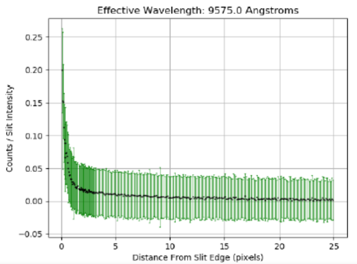
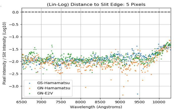
We do not construct a similar model of light outside of alignment star boxes. This requires some additional work and given that only a small subset of our data will be affected, we did not do it. Another deficiency is that this model assumes the scattered light is dominated by sky emission within the slit, as is generally the case, at least at the location of bright sky lines. If the source itself is bright, there is an additional contribution, that may be asymmetric between the two pairs of slits because the object is nodded along the spatial direction. This has a particularly notable effect on band-shuffle masks, which normally should not be affected by this charge leakage. In the band-shuffled case, one set of spectra (corresponding to the A position) are at one end of the detector, and the other set are at the opposite end. The scattered light pattern is the same in both, and generally subtracts off without problem. This isn’t true if the science target contributes significantly to the flux. In particular it is a problem for the mask alignment boxes; these contain bright stars in the A position, but they are mostly nodded out of the box in the B position. Where these contribute to the scattered light, they lead to an asymmetry in the two sets of spectra. The problem becomes acute because, compared with microshuffle observations, the same number (3–4) of alignment stars are packed into a third of the area; thus there is a greater contamination of neighbouring slits. Our procedure does not correct for this, and it means that spectra near alignment star boxes in band-shuffle masks still suffer from this effect.

Having constructed the parametric model, we then apply it to both sides of every spectrum on every GOGREEN mask, and subtract off the estimated contribution. The result of our correction is quantitatively quite excellent for most spectra. The right panels of Figure 13 show the same detector regions as before, at the same contrast, but after the correction has been applied. A quantitative comparison is shown in Figure 16, which shows the residual intensity at a distance of five pixels from the slit edge, as a function of wavelength. One set of points corresponds to the original data, and the other is after we have applied our correction. This empirical correction is not perfect, and fails for a small percentage of slits, particularly those near alignment star boxes. However, the improvement for most of the data is significant and employing the correction enables redshift and line index measurements for hundreds of additional galaxies.

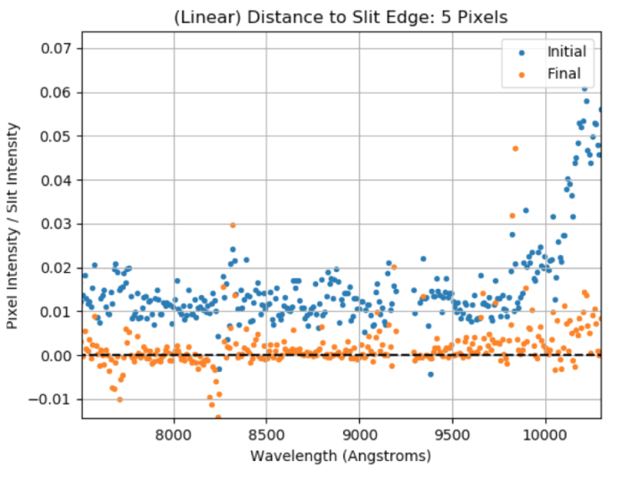
Uncertainties related to this correction are estimated from the variance in residuals and added to the variance vectors propagated through the data reduction procedure.

Appendix C GOGREEN Telluric corrections

To model and correct the telluric absorption in the GOGREEN spectra we use the ESO code molecfit (Kausch et al., 2014; Smette et al., 2015). First, this code reads the science spectrum and a set of ambient input parameters. Then, it creates a single profile of the Earth’s atmosphere at the time of observation by gathering data from three sources: ENVISAT, GDAS, and the corresponding ground-based ESO Meteo Monitor measurements. The next step is the construction of a synthetic atmospheric absorption model by fitting user-defined spectral regions dominated by telluric absorption, for which molecfit relies on the radiative transfer code LBLRTM. In particular, we fit the spectral regions $\lambda\lambda\,$ 6780,7000; $\lambda\lambda\,$ 7110,7750; $\lambda\lambda\,$ 8050,8450; and, $\lambda\lambda\,$ 8770, 10020 Å, where strong H₂O, O₂, and O₃ telluric features are found, as shown in Figure 17. We exclude regions from the fit if they coincide with a strong spectral feature in the spectrum, such as an [Oii] emission line. The code modifies the model spectrum, using a polynomial fit of the continuum and the wavelength grid of each spectral region and convolving it with a kernel mimicking the instrumental profile, to match the science spectrum. The fitting of the science and the model spectrum is performed by the mpfit package, which uses a $\chi^{2}$ minimization procedure based on the Levenberg-Marquard iterative technique. If the desired fit quality is not reached, mpfit changes the fit parameters (e.g., molecular abundances) to search for a better $\chi^{2}$ . Finally, the atmospheric transmission model for the full wavelength range of the input science spectrum is calculated.

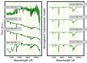
Appendix D Spectral flux calibration

As described in § 3.2, the wavelength dependence of the spectral flux calibration is calibrated using standard star observations. However this does not account for slit losses and atmospheric effects that reduce the overall amplitude of the final spectrum. To obtain an absolute flux calibration for the GOGREEN and GCLASS spectra, we use $i$ -band photometric data described in Section 6.3. We use the Suprime-Cam $i$ -band for northern clusters and VIMOS $i$ -band for the southern clusters. The filter response curve, $R$ , is interpolated using a cubic-spline to match the wavelength sampling of the spectroscopy. We then integrate over the interpolated filter response curve multiplied by the spectral flux density to give the average spectral flux density, in $\rm{erg\;cm^{-2}s^{-1}}$ Å^-1:

\displaystyle f_{\rm\lambda,tot,spec}=\int_{\lambda_{\rm min}}^{\lambda_{\rm max}}(R\,f_{\lambda}\,\lambda\,d\lambda)/\int_{\lambda_{\rm min}}^{\lambda_{\rm max}}(R\,\lambda\,d\lambda).

(2)

In this calculation, regions of the spectroscopy flagged as bad data are omitted. The synthetic photometric flux in Jy is then determined as

\displaystyle f_{\rm\nu,tot,spec}=3.34\times 10^{4}\;\lambda_{\rm pivot}^{2}\;f_{\rm\lambda,tot,spec}\;,

(3)

where the pivot wavelength

\displaystyle\lambda_{\rm pivot}=\sqrt{\int_{\lambda_{\rm min}}^{\lambda_{\rm max}}{R\,\lambda\,d\lambda}/\int_{\lambda_{\rm min}}^{\lambda_{\rm max}}{R/\lambda\,d\lambda}}

(4)

Finally, we compare this flux with the total i-band flux from the photometric catalogues $f_{\rm\nu,tot,phot}$ , to obtain a flux calibration ratio

\displaystyle f_{\rm cal}=f_{\rm\nu,tot,spec}/f_{\rm\nu,tot,phot}

(5)

The flux calibrated spectrum and variance are then calculated as:

	$\displaystyle f_{\rm\lambda,cal}=f_{\rm\lambda}/f_{\rm cal},$		(6)
	$\displaystyle Var(f_{\rm\lambda,cal})=Var(f_{\rm\lambda})/(f_{\rm cal})^{2}.$		(7)

Appendix E Spectroscopic completeness

Here we describe in more detail our method for estimating the spectroscopic incompleteness of the GOGREEN sample, as a function of the galaxy position in the color magnitude diagram and of the galaxy distance from the cluster center.

To compute the incompleteness as a function of the position on the color-magnitude diagram, we first subdivided the diagram of each field into cells and then we compared the number of objects in the spectroscopic catalog with the number in the parent photometric catalog. The parent catalog included all entries in the GOGREEN photometric catalog that were retained as targets for spectroscopy. The ratio of these two numbers yielded a weight as a function of galaxy apparent magnitude and color (W_mag). As the target selection in the $z^{\prime}{-[}3.6$ ] vs [3.6] plane was slightly different from cluster to cluster, depending on the redshift of the cluster, we first computed these weights field by field instead of binning all fields together.

We also quantified the presence of geometrical effects due to possible variations in the sampling as a function of the clustercentric radius. Geometrical effects can affect a spectroscopic sample of a cluster due to the fact that cluster galaxies are indeed more concentrated toward the cluster center, so observational constraints on the minimum distance between slits typically result in a lower sampling of these central regions. The geometrical completeness W_geo was computed comparing the number of galaxies in the spectroscopic and in the parent photometric catalogs in four annuli with R < 0.6, 0.6 < R < 1.2, 1.2 < R < 2, and R > 2 in units of R₂₀₀. Figures 18-29 show the completeness diagrams for the clusters in the sample. The results for the combined sample are given in the main body of the paper, in Figure 10.

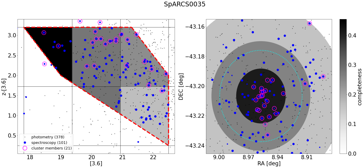
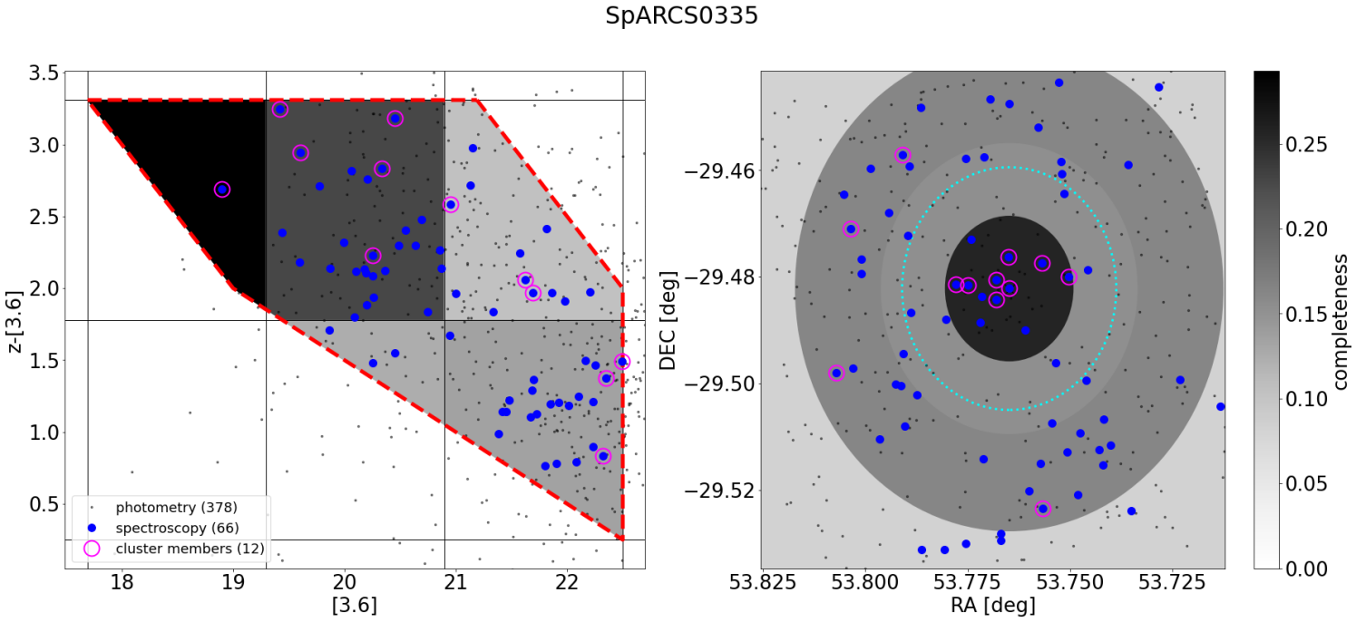
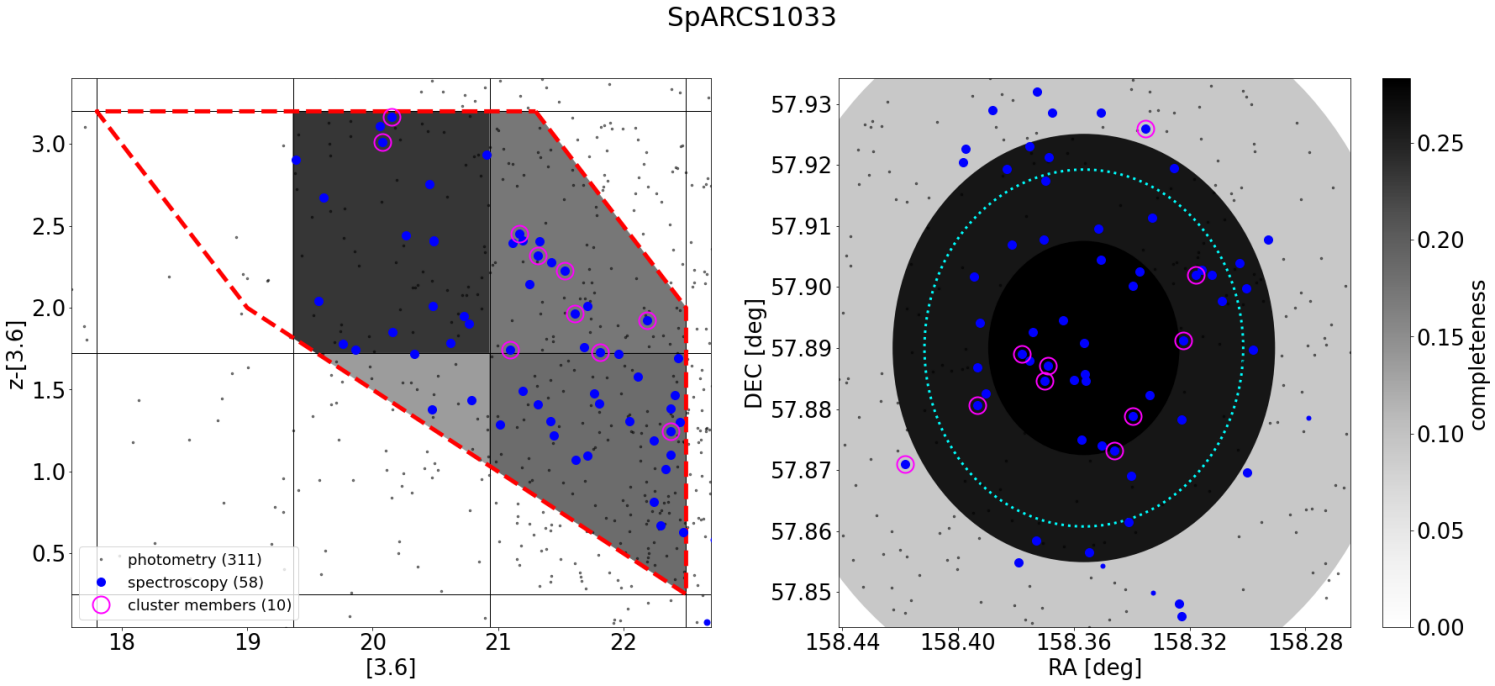
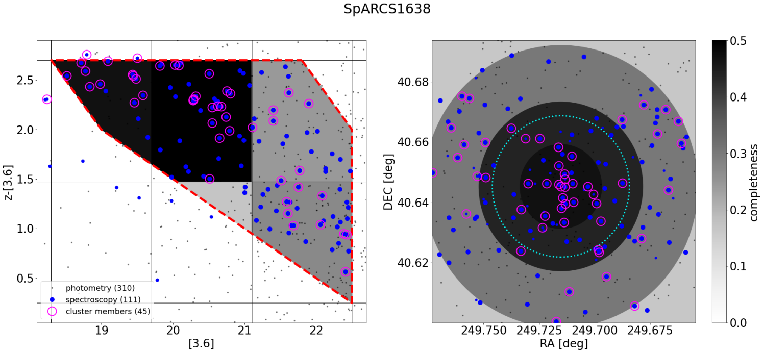
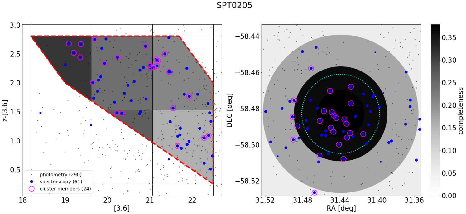
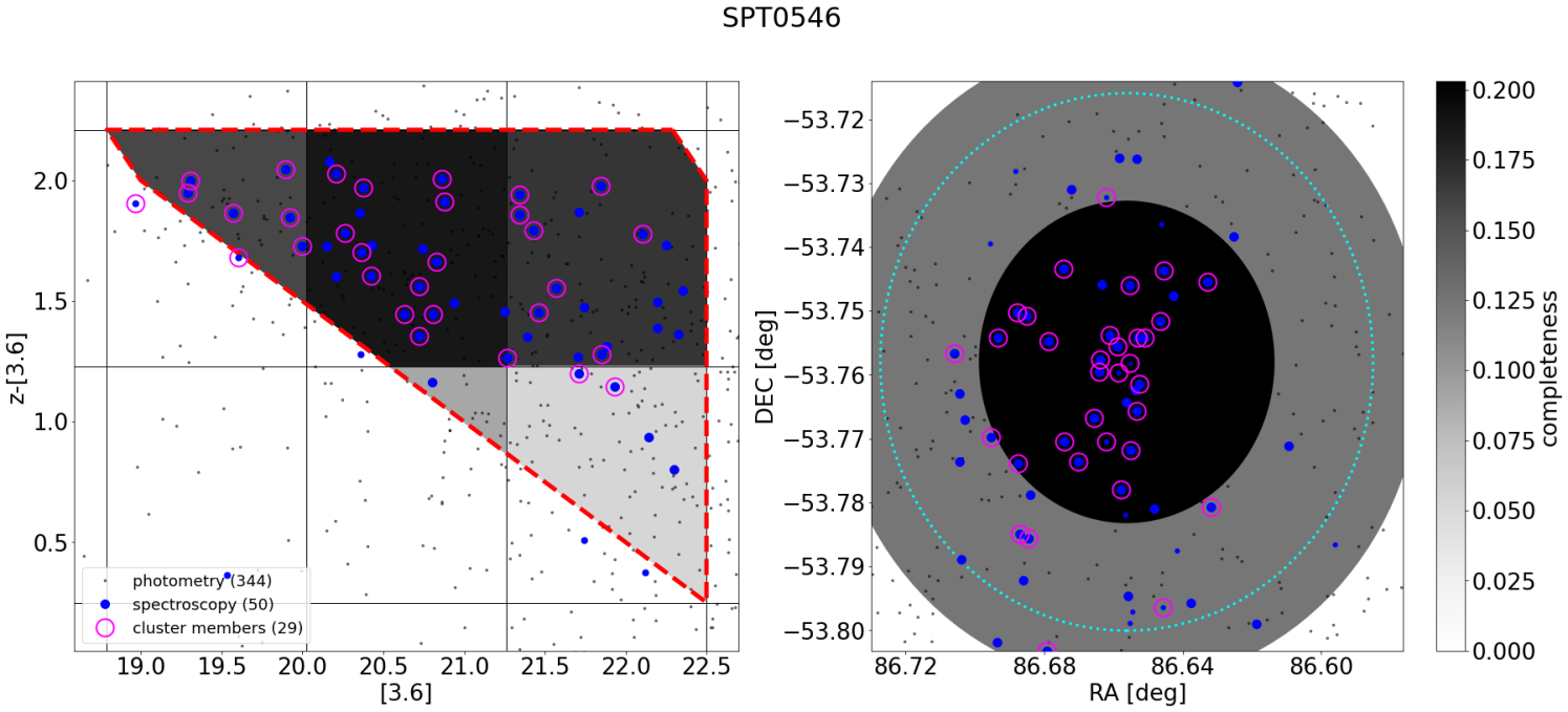
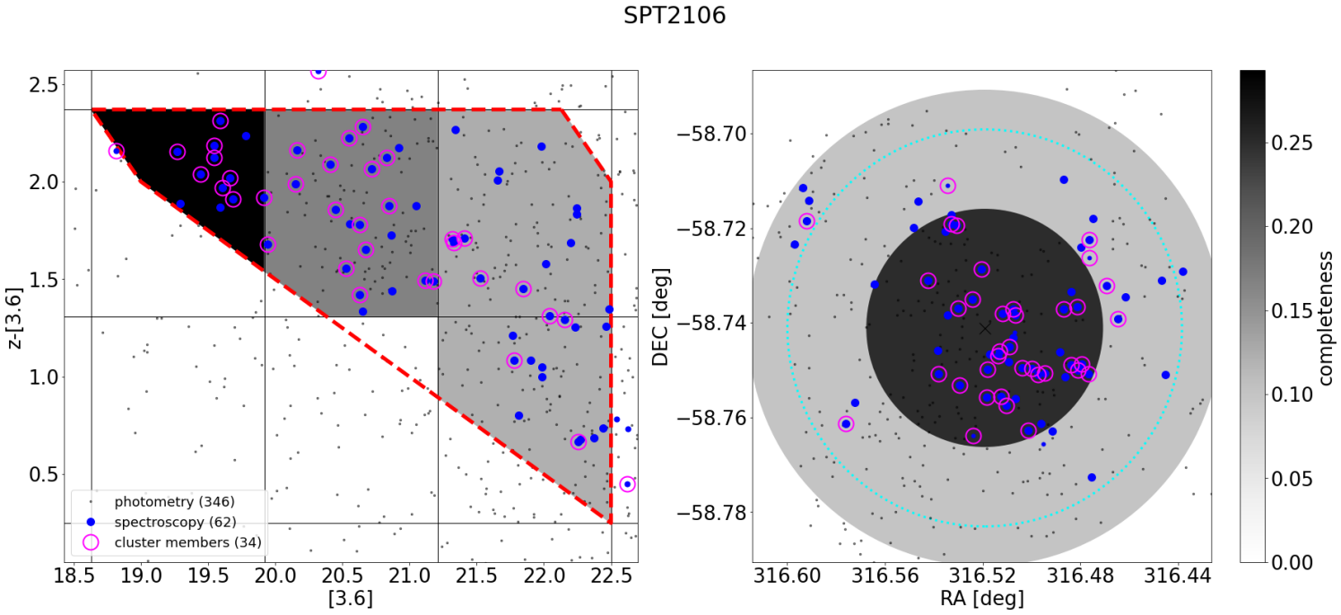
Appendix F Spectroscopy Log

Table LABEL:tab-specobs provides a log of all GOGREEN spectroscopy obtained as part of this program. We identify the dates of observation, mask name, nod-and-shuffle mode (microshuffle or bandshuffle), telescope/detector combination, total integration time, and whether the data were taken in Queue mode.

Table 8: A log of all spectroscopic data obtained for GOGREEN. All data were acquired in Priority Visitor mode unless otherwise indicated in the Final column.

Target	Date	Mask	Band/Micro	Telescope/	Integration	Notes
				Detector	time (ks)
SPT0205	Nov 16,18, 2014	GS2014BLP001-06	Microshuffle	GS/Ham	6.48
	Oct 29-30, Nov 3 2016	GS2016BLP001-02	Microshuffle	GS/Ham	10.8
	Oct 28-29, 2016	GS2016BLP001-09	Microshuffle	GS/Ham	9.36
	Nov 13, 2017	GS2017BLP001-03	Microshuffle	GS/Ham	8.64	GS2017BDD10
	Nov 14, 2017	GS2017BLP001-04	Microshuffle	GS/Ham	10.8
	Jan 10, 16, 18, 2018	GS2017BLP001-03	Microshuffle	GS/Ham	10.8
SPT0546	Nov 15-16, 2014	GS2014BLP001-09	Microshuffle	GS/Ham	5.76
	Nov 17,19, 2014	GS2014BLP001-10	Microshuffle	GS/Ham	7.2
	Nov 20, 2015	GS2015BLP001-15	Microshuffle	GS/Ham	7.92
	Nov 21, 2015	GS2015BLP001-16	Microshuffle	GS/Ham	2.16
	Feb 10, 2016	GS2015BLP001-16	Microshuffle	GS/Ham	14.4
	Nov 13-14, 16, 2017	GS2017BLP001-12	Microshuffle	GS/Ham	9.36
	Nov 15-16, 2017	GS2017BLP001-13	Microshuffle	GS/Ham	10.08
SPT2106	June 15, 2018	GS2018ALP001-01	Microshuffle	GS/Ham	10.8	Queue
	June 16-17, 2018	GS2018ALP001-02	Microshuffle	GS/Ham	10.8	Queue
	Sept 6, 2018	GS2018BLP001-04	Microshuffle	GS/Ham	10.8
	Sept 7, 2018	GS2018BLP001-05	Microshuffle	GS/Ham	10.8
SpARCS0035	Nov 21, 2015	GS2015BLP001-05	Bandshuffle	GS/Ham	9.36
	Nov 20, 2015	GS2015BLP001-06	Microshuffle	GS/Ham	7.2
	Oct 28, 2016	GS2016BLP001-01	Microshuffle	GS/Ham	7.9
	Oct 27, 2016	GS2016BLP001-07	Microshuffle	GS/Ham	10.8
	Nov 11, 2017	GS2017BLP001-01	Microshuffle	GS/Ham	7.9
	Nov 12, 2017	GS2017BLP001-02	Microshuffle	GS/Ham	10.8
SpARCS0219	Nov 20, 2015	GS2015BLP001-17	Microshuffle	GS/Ham	10.8
	Oct 30, 2016	GS2016BLP001-03	Microshuffle	GS/Ham	8.64
	Oct 27-28, 2016	GS2016BLP001-12	Microshuffle	GS/Ham	9.36
	Nov 15, 2017	GS2017BLP001-11	Microshuffle	GS/Ham	9.36
SpARCS0335	Nov 18-19, 2014	GS2014BLP001-01	Bandshuffle	GS/Ham	7.2
	Feb 1, 2017	GS2016BLP001-13	Bandshuffle	GS/Ham	9.36
	Oct 26-29, 2016	GS2016BLP001-14	Bandshuffle	GS/Ham	10.8
	Nov 11, 2017	GS2017BLP001-07	Microshuffle	GS/Ham	7.92
	Nov 12-13, 2017	GS2017BLP001-08	Microshuffle	GS/Ham	8.64
SpARCS1051	Feb 18&29, 2016	GN2016ALP004-03	Microshuffle	GN/EEV	18.0	Queue
	April 25, 2017	GN2017ALP004-08	Microshuffle	GN/Ham	12.0
	April 26, 2017	GN2017ALP004-07	Microshuffle	GN/Ham	13.8
	Feb 12, 2018	GN2018ALP004-07	Microshuffle	GN/Ham	13.68
SpARCS1033	April 18, 2017	GN2017ALP004-01	Bandshuffle	GN/Ham	7.2
	April 19, 2017	GN2017ALP004-02	Microshuffle	GN/Ham	10.08
	April 20, 2017	GN2017ALP004-03	Microshuffle	GN/Ham	10.08
	Feb 11, 2018	GN2018ALP004-01	Microshuffle	GN/Ham	7.92
	Feb 11, 13 2018	GN2018ALP004-02	Microshuffle	GN/Ham	7.92
SpARCS1034	April 24, 2017	GN2017ALP004-04	Bandshuffle	GN/Ham	4.3
	April 12&27, 2017	GN2017ALP004-05	Bandshuffle	GN/Ham	10.08
	May 21,22, 29, 31, June 3, 2017	GN2017ALP004-06	Microshuffle	GN/Ham	10.8	Queue
	Feb 13 2018	GN2018ALP004-04	Microshuffle	GN/Ham	9.36
	Feb 17, June 12, 2018	GN2018ALP004-05	Microshuffle	GN/Ham	7.2
SpARCS1616	June 1, 2016	GN2016ALP004-06	Microshuffle	GN/EEV	14.4
	June 2, 2016	GN2016ALP004-07	Microshuffle	GN/EEV	18.0
	April 18&27, 2017	GN2017ALP004-09	Microshuffle	GN/Ham	17.28
	June 10, 12, 2018	GN2018ALP004-08	Microshuffle	GN/Ham	17.28
SpARCS1634	May 30, 2016	GN2016ALP004-04	Microshuffle	GN/EEV	10.8
	May 30-31, 2016	GN2016ALP004-05	Microshuffle	GN/EEV	18.0
	April 19/26, 2017	GN2017ALP004-10	Microshuffle	GN/Ham	18.0
	June 12-13, 2018	GN2018ALP004-09	Microshuffle	GN/Ham	17.28
SpARCS1638	May 28-20, 2016	GN2016ALP004-01	Microshuffle	GN/EEV	10.8
	May 29/June2, 2016	GN2016ALP004-02	Microshuffle	GN/EEV	18.0
	April 20/28, 2017	GN2017ALP004-11	Microshuffle	GN/Ham	18.0
	June 21-23, 2018	GN2018ALP004-10	Microshuffle	GN/Ham	19.44
COSMOS-28	Jan 30, 2016	GN2015BLP004-03	Microshuffle	GN/EEV	18.0	Queue
	Mar 4,6, 2019	GN2019ALP004-01	Microshuffle	GN/Ham	20.88	Queue
	April 7, 24-26, 2019	GN2019ALP004-02	Microshuffle	GN/Ham	19.44	Queue
	April 27, May 1, 8, 10-11, 2019	GN2019ALP004-03	Microshuffle	GN/Ham	19.44	Queue
COSMOS-63	Jan 31, 2016	GN2015BLP004-02	Microshuffle	GN/EEV	18.0	Queue
COSMOS-125	Jan 31, 2016	GS2016ALP001-02	Microshuffle	GS/Ham	15.12
	Feb 25, 2015	GS2015ALP001-02	Microshuffle	GS/Ham	12.25
COSMOS-221	Feb 24, 2015	GS2015ALP001-01	Microshuffle	GS/Ham	10.08
	Feb 23, 2015	GS2014BLP001-05	Microshuffle	GS/Ham	5.04
	Feb 13, 2016	GS2016ALP001-01	Microshuffle	GS/Ham	10.8
SXDF49/87	Oct 9, 2015	GN2015BLP004-01	Microshuffle	GN/EEV	18.0	Queue
	Nov 15, 2014	GS2014BLP001-07	Microshuffle	GS/Ham	8.64
	Nov 1, 2018	GN2018BLP004-01	Microshuffle	GN/Ham	10.8
	Sept 6, 2018	GS2018BLP001-01	Microshuffle	GS/Ham	12.96
	Sept 8, 2018	GS2018BLP001-02	Microshuffle	GS/Ham	12.96
	Sept 7, 9, 2018	GS2018BLP001-03	Microshuffle	GS/Ham	12.24
SXDF64	Nov 17, 2014	GS2014BLP001-08	Microshuffle	GS/Ham	7.2
SXDF76	Nov 15, 2014	GS2014BLP001-02	Microshuffle	GS/Ham	5.76
	Nov 5, 2018	GN2018BLP004-02	Microshuffle	GN/Ham	15.12
	Nov 5, 2018	GN2018BLP004-03	Microshuffle	GN/Ham	15.12
	Nov 6, 12, 2018	GN2018BLP004-04	Microshuffle	GN/Ham	15.12

References

Abraham et al. (1996) Abraham R. G., et al., 1996, ApJ, 471, 694
Abraham et al. (2004) Abraham R. G., et al., 2004, AJ, 127, 2455
Balogh et al. (1997) Balogh M. L., Morris S. L., Yee H. K. C., Carlberg R. G., Ellingson E., 1997, ApJL, 488, L75+
Balogh et al. (1998) Balogh M. L., Schade D., Morris S. L., Yee H. K. C., Carlberg R. G., Ellingson E., 1998, ApJ, 504, L75
Balogh et al. (1999) Balogh M. L., Morris S. L., Yee H. K. C., Carlberg R. G., Ellingson E., 1999, ApJ, 527, 54
Balogh et al. (2011) Balogh M. L., et al., 2011, MNRAS, 412, 2303
Balogh et al. (2014) Balogh M. L., et al., 2014, MNRAS, 443, 2679
Balogh et al. (2016) Balogh M. L., et al., 2016, MNRAS, 456, 4364
Balogh et al. (2017) Balogh M. L., et al., 2017, MNRAS, 470, 4168
Bayliss et al. (2016) Bayliss M. B., et al., 2016, ApJS, 227, 3
Beers et al. (1990) Beers T. C., Flynn K., Gebhardt K., 1990, AJ, 100, 32
Beers et al. (1991) Beers T. C., Gebhardt K., Forman W., Huchra J. P., Jones C., 1991, AJ, 102, 1581
Bertin (2011) Bertin E., 2011, in Evans I. N., Accomazzi A., Mink D. J., Rots A. H., eds, Astronomical Society of the Pacific Conference Series Vol. 442, Astronomical Data Analysis Software and Systems XX. p. 435
Bertin & Arnouts (1996) Bertin E., Arnouts S., 1996, A&AS, 117, 393
Biviano et al. (2016) Biviano A., van der Burg R. F. J., Muzzin A., Sartoris B., Wilson G., Yee H. K. C., 2016, A&A, 594, A51
Bleem et al. (2020) Bleem L. E., et al., 2020, ApJS, 247, 25
Bradshaw et al. (2013) Bradshaw E., et al., 2013, Monthly Notices of the Royal Astronomical Society, 433, 194
Brammer et al. (2008) Brammer G. B., van Dokkum P. G., Coppi P., 2008, ApJ, 686, 1503
Brodwin et al. (2010) Brodwin M., et al., 2010, ApJ, 721, 90
Brodwin et al. (2013) Brodwin M., et al., 2013, ApJ, 779, 138
Bruzual & Charlot (2003) Bruzual G., Charlot S., 2003, MNRAS, 344, 1000
Butcher & Oemler (1978a) Butcher H., Oemler A., 1978a, ApJ, 219, 18
Butcher & Oemler (1978b) Butcher H., Oemler A., 1978b, ApJ, 226, 559
Carlberg et al. (1996) Carlberg R. G., Yee H. K. C., Ellingson E., Abraham R., Gravel P., Morris S., Pritchet C. J., 1996, ApJ, 462, 32
Chabrier (2003) Chabrier G., 2003, PASP, 115, 763
Chan et al. (2019) Chan J. C. C., et al., 2019, ApJ, 880, 119
Chiappetti et al. (2013) Chiappetti L., et al., 2013, MNRAS, 429, 1652
Colless et al. (2001) Colless M., et al., 2001, MNRAS, 328, 1039
De Lucia et al. (2007) De Lucia G., et al., 2007, MNRAS, 374, 809
De Lucia et al. (2009) De Lucia G., Poggianti B. M., Halliday C., Milvang-Jensen B., Noll S., Smail I., Zaritsky D., 2009, MNRAS, 400, 68
De Propris et al. (2002) De Propris R., et al., 2002, MNRAS, 329, 87
De Propris et al. (2004) De Propris R., et al., 2004, MNRAS, 351, 125
Delahaye et al. (2017) Delahaye A. G., et al., 2017, ApJ, 843, 126
Demarco et al. (2010) Demarco R., et al., 2010, ApJ, 711, 1185
Desai et al. (2007) Desai V., et al., 2007, ApJ, 660, 1151
Dressler et al. (1997) Dressler A., et al., 1997, ApJ, 490, 577
Dressler et al. (1999) Dressler A., Smail I., Poggianti B. M., Butcher H., Couch W. J., Ellis R. S., Oemler Augustus J., 1999, ApJS, 122, 51
Dressler et al. (2013) Dressler A., Oemler Augustus J., Poggianti B. M., Gladders M. D., Abramson L., Vulcani B., 2013, ApJ, 770, 62
Eisenhardt et al. (2008) Eisenhardt P. R. M., et al., 2008, ApJ, 684, 905
Ellingson et al. (2001) Ellingson E., Lin H., Yee H. K. C., Carlberg R. G., 2001, ApJ, 547, 609
Ellis et al. (1996) Ellis R. S., Colless M., Broadhurst T., Heyl J., Glazebrook K., 1996, MNRAS, 280, 235
Ellis et al. (2014) Ellis S. C., Saunders W., Betters C., Croom S., 2014, in Proc. SPIE. p. 91511V, doi:10.1117/12.2057108
Finn et al. (2005) Finn R. A., et al., 2005, ApJ, 630, 206
Finoguenov et al. (2007) Finoguenov A., et al., 2007, ApJS, 172, 182
Finoguenov et al. (2010) Finoguenov A., et al., 2010, MNRAS, 403, 2063
Foley et al. (2011) Foley R. J., et al., 2011, ApJ, 731, 86
Foltz et al. (2015) Foltz R., et al., 2015, ApJ, 812, 138
Foltz et al. (2018) Foltz R., et al., 2018, ApJ, 866, 136
Gómez et al. (2003) Gómez P. L., et al., 2003, ApJ, 584, 210
Galametz et al. (2013) Galametz A., et al., 2013, ApJS, 206, 10
George et al. (2011) George M. R., et al., 2011, ApJ, 742, 125
Gilbank et al. (2010) Gilbank D. G., Baldry I. K., Balogh M. L., Glazebrook K., Bower R. G., 2010, MNRAS, 405, 2594
Gilbank et al. (2011) Gilbank D. G., Gladders M. D., Yee H. K. C., Hsieh B. C., 2011, AJ, 141, 94
Gimeno et al. (2016) Gimeno G., et al., 2016, in Evans C. J., Simard L., Takami H., eds, Vol. 9908, Ground-based and Airborne Instrumentation for Astronomy VI. SPIE, pp 872 – 885, doi:10.1117/12.2233883, https://doi.org/10.1117/12.2233883
Gladders & Yee (2000) Gladders M. D., Yee H. K. C., 2000, AJ, 120, 2148
Gladders & Yee (2005) Gladders M. D., Yee H. K. C., 2005, ApJS, 157, 1
Gonzaga et al. (2012) Gonzaga S., et al. B C 2012, The DrizzlePac Handbook
Gonzalez et al. (2019) Gonzalez A. H., et al., 2019, ApJS, 240, 33
Guglielmo et al. (2015) Guglielmo V., Poggianti B. M., Moretti A., Fritz J., Calvi R., Vulcani B., Fasano G., Paccagnella A., 2015, MNRAS, 450, 2749
Guglielmo et al. (2018) Guglielmo V., et al., 2018, A&A, 620, A7
Guglielmo et al. (2019) Guglielmo V., et al., 2019, A&A, 625, A112
Gullieuszik et al. (2015) Gullieuszik M., et al., 2015, A&A, 581, A41
Halliday et al. (2004) Halliday C., et al., 2004, A&A, 427, 397
High et al. (2009) High F. W., Stubbs C. W., Rest A., Stalder B., Challis P., 2009, AJ, 138, 110
Hinton et al. (2016) Hinton S. R., Davis T. M., Lidman C., Glazebrook K., Lewis G. F., 2016, Astronomy and Computing, 15, 61
Hook et al. (2004) Hook I. M., Jørgensen I., Allington-Smith J. R., Davies R. L., Metcalfe N., Murowinski R. G., Crampton D., 2004. pp 425–440, doi:10.1086/383624
Hou et al. (2013) Hou A., et al., 2013, MNRAS, 435, 1715
Ivanov et al. (2004) Ivanov V. D., Rieke M. J., Engelbracht C. W., Alonso-Herrero A., Rieke G. H., Luhman K. L., 2004, ApJS, 151, 387
Jarrett et al. (2000) Jarrett T. H., Chester T., Cutri R., Schneider S., Skrutskie M., Huchra J. P., 2000, AJ, 119, 2498
Kausch et al. (2014) Kausch W., et al., 2014, in Manset N., Forshay P., eds, Astronomical Society of the Pacific Conference Series Vol. 485, Astronomical Data Analysis Software and Systems XXIII. p. 403 (arXiv:1401.7768)
Kelly et al. (2014) Kelly P. L., et al., 2014, MNRAS, 439, 28
Khullar et al. (2019) Khullar G., et al., 2019, ApJ, 870, 7
Kriek et al. (2009) Kriek M., van Dokkum P. G., Labbé I., Franx M., Illingworth G. D., Marchesini D., Quadri R. F., 2009, ApJ, 700, 221
Kurk et al. (2013) Kurk J., et al., 2013, A&A, 549, A63
Le Fèvre et al. (2005) Le Fèvre O., et al., 2005, A&A, 439, 845
Le Fèvre et al. (2015) Le Fèvre O., et al., 2015, A&A, 576, A79
Leja et al. (2019) Leja J., Carnall A. C., Johnson B. D., Conroy C., Speagle J. S., 2019, ApJ, 876, 3
Lewis et al. (2002) Lewis I., et al., 2002, MNRAS, 334, 673
Lidman et al. (2008) Lidman C., et al., 2008, A&A, 489, 981
Lidman et al. (2012) Lidman C., et al., 2012, MNRAS, 427, 550
Lidman et al. (2013) Lidman C., et al., 2013, MNRAS, 433, 825
Lilly et al. (1996) Lilly S. J., Le Fevre O., Hammer F., Crampton D., 1996, ApJ, 460, L1
Lilly et al. (2009) Lilly S. J., et al., 2009, ApJS, 184, 218
Lin et al. (2017) Lin Y.-T., et al., 2017, ApJ, 851, 139
Lonsdale et al. (2003) Lonsdale C. J., et al., 2003, PASP, 115, 897
Mamon et al. (2013) Mamon G. A., Biviano A., Boué G., 2013, MNRAS, 429, 3079
Matharu et al. (2019) Matharu J., et al., 2019, MNRAS, 484, 595
Mauduit et al. (2012) Mauduit J.-C., et al., 2012, PASP, 124, 714
McCracken et al. (2012) McCracken H. J., et al., 2012, A&A, 544, A156
McLachlan & Basford (1988) McLachlan G. J., Basford K. E., 1988, Mixture models. Inference and applications to clustering
McLure et al. (2012) McLure R., et al., 2012, Monthly Notices of the Royal Astronomical Society, 428, 1088
Mehta et al. (2018) Mehta V., et al., 2018, ApJS, 235, 36
Melnyk et al. (2013) Melnyk O., et al., 2013, A&A, 557, A81
Milvang-Jensen et al. (2008) Milvang-Jensen B., et al., 2008, A&A, 482, 419
Mok et al. (2013) Mok A., et al., 2013, MNRAS, 431, 1090
Mok et al. (2014) Mok A., et al., 2014, MNRAS, 438, 3070
Monet et al. (2003) Monet D. G., et al., 2003, AJ, 125, 984
Moretti et al. (2017) Moretti A., et al., 2017, A&A, 599, A81
Muzzin et al. (2009) Muzzin A., et al., 2009, ApJ, 698, 1934
Muzzin et al. (2012) Muzzin A., et al., 2012, ApJ, 746, 188
Muzzin et al. (2013) Muzzin A., et al., 2013, ApJS, 206, 8
Muzzin et al. (2014) Muzzin A., et al., 2014, ApJ, 796, 65
Nantais et al. (2016) Nantais J. B., et al., 2016, A&A, 592, A161
Nantais et al. (2017) Nantais J. B., et al., 2017, MNRAS, 465, L104
Newman et al. (2013) Newman J. A., et al., 2013, ApJS, 208, 5
Noble et al. (2013) Noble A. G., Webb T. M. A., Muzzin A., Wilson G., Yee H. K. C., van der Burg R. F. J., 2013, ApJ, 768, 118
Noble et al. (2016) Noble A. G., Webb T. M. A., Yee H. K. C., Muzzin A., Wilson G., van der Burg R. F. J., Balogh M. L., Shupe D. L., 2016, ApJ, 816, 48
Oemler et al. (2013) Oemler Augustus J., et al., 2013, ApJ, 770, 61
Old et al. (2020) Old L. J., et al., 2020, MNRAS, 493, 5987
Paccagnella et al. (2017) Paccagnella A., et al., 2017, ApJ, 838, 148
Pentericci et al. (2018) Pentericci L., McLure R. J., Franzetti P., Garilli B., the VANDELS team 2018, arXiv e-prints, p. arXiv:1811.05298
Pickles (1998) Pickles A. J., 1998, PASP, 110, 863
Pintos-Castro et al. (2019) Pintos-Castro I., Yee H. K. C., Muzzin A., Old L., Wilson G., 2019, ApJ, 876, 40
Poggianti et al. (1999) Poggianti B. M., Smail I., Dressler A., Couch W. J., Barger A. J., Butcher H., Ellis R. S., Oemler Augustus J., 1999, ApJ, 518, 576
Poggianti et al. (2006) Poggianti B., et al., 2006, ApJ, 642, 188
Poggianti et al. (2008) Poggianti B. M., et al., 2008, ApJ, 684, 888
Poggianti et al. (2009) Poggianti B. M., et al., 2009, ApJ, 693, 112
Quadri et al. (2012) Quadri R. F., Williams R. J., Franx M., Hildebrandt H., 2012, ApJ, 744, 88
Rudnick et al. (2009) Rudnick G., et al., 2009, ApJ, 700, 1559
Ruel et al. (2014) Ruel J., et al., 2014, ApJ, 792, 45
Sanders et al. (2007) Sanders D. B., et al., 2007, ApJS, 172, 86
Saro et al. (2013) Saro A., Mohr J. J., Bazin G., Dolag K., 2013, ApJ, 772, 47
Schlegel et al. (1998) Schlegel D. J., Finkbeiner D. P., Davis M., 1998, ApJ, 500, 525
Scodeggio et al. (2018) Scodeggio M., et al., 2018, A&A, 609, A84
Sifón et al. (2013) Sifón C., et al., 2013, ApJ, 772, 25
Sifón et al. (2016) Sifón C., et al., 2016, MNRAS, 461, 248
Smette et al. (2015) Smette A., et al., 2015, A&A, 576, A77
Stalder et al. (2013) Stalder B., et al., 2013, ApJ, 763, 93
Tomczak et al. (2014) Tomczak A. R., et al., 2014, ApJ, 783, 85
Vulcani et al. (2010) Vulcani B., Poggianti B. M., Finn R. A., Rudnick G., Desai V., Bamford S., 2010, ApJL, 710, L1
Vulcani et al. (2011) Vulcani B., et al., 2011, MNRAS, 412, 246
White et al. (2005) White S. D. M., et al., 2005, A&A, 444, 365
Williams et al. (2009) Williams R. J., Quadri R. F., Franx M., van Dokkum P., Labbé I., 2009, ApJ, 691, 1879
Wilson et al. (2009) Wilson G., et al., 2009, ApJ, 698, 1943
Woods et al. (1994) Woods T. N., Wrigley R. T., Rottman G. J., Haring R. E., 1994, Appl. Opt., 33, 4273
Yee et al. (1996) Yee H. K. C., Ellingson E., Carlberg R. G., 1996, ApJS, 102, 269
York et al. (2000) York D. G., et al., 2000, AJ, 120, 1579
van der Burg et al. (2010) van der Burg R. F. J., Hildebrandt H., Erben T., 2010, A&A, 523, A74
van der Burg et al. (2013) van der Burg R. F. J., et al., 2013, A&A, 557, A15
van der Burg et al. (2014) van der Burg R. F. J., Muzzin A., Hoekstra H., Wilson G., Lidman C., Yee H. K. C., 2014, A&A, 561, A79
van der Burg et al. (2020) van der Burg R. F. J., et al., 2020, A&A, 638, A112